Guest post by Pat Frank
Readers of Watts Up With That will know from Mark I that for six years I have been trying to publish a manuscript with the post title. Well, it has passed peer review and is now published at Frontiers in Earth Science: Atmospheric Science. The paper demonstrates that climate models have no predictive value.
Before going further, my deep thanks to Anthony Watts for giving a voice to independent thought. So many have sought to suppress it (freedom denialists?). His gift to us (and to America) is beyond calculation. And to Charles the moderator, my eternal gratitude for making it happen.
Onward: the paper is open access. It can be found here , where it can be downloaded; the Supporting Information (SI) is here (7.4 MB pdf).
I would like to publicly honor my manuscript editor Dr. Jing-Jia Luo, who displayed the courage of a scientist; a level of professional integrity found lacking among so many during my 6-year journey.
Dr. Luo chose four reviewers, three of whom were apparently not conflicted by investment in the AGW status-quo. They produced critically constructive reviews that helped improve the manuscript. To these reviewers I am very grateful. They provided the dispassionate professionalism and integrity that had been in very rare evidence within my prior submissions.
So, all honor to the editors and reviewers of Frontiers in Earth Science. They rose above the partisan and hewed the principled standards of science when so many did not, and do not.
A digression into the state of practice: Anyone wishing a deep dive can download the entire corpus of reviews and responses for all 13 prior submissions, here (60 MB zip file, Webroot scanned virus-free). Choose “free download” to avoid advertising blandishment.
Climate modelers produced about 25 of the prior 30 reviews. You’ll find repeated editorial rejections of the manuscript on the grounds of objectively incompetent negative reviews. I have written about that extraordinary reality at WUWT here and here. In 30 years of publishing in Chemistry, I never once experienced such a travesty of process. For example, this paper overturned a prediction from Molecular Dynamics and so had a very negative review, but the editor published anyway after our response.
In my prior experience, climate modelers:
· did not know to distinguish between accuracy and precision.
· did not understand that, for example, a ±15 C temperature uncertainty is not a physical temperature.
· did not realize that deriving a ±15 C uncertainty to condition a projected temperature does *not* mean the model itself is oscillating rapidly between icehouse and greenhouse climate predictions (an actual reviewer objection).
· confronted standard error propagation as a foreign concept.
· did not understand the significance or impact of a calibration experiment.
· did not understand the concept of instrumental or model resolution or that it has empirical limits
· did not understand physical error analysis at all.
· did not realize that ‘±n’ is not ‘+n.’
Some of these traits consistently show up in their papers. I’ve not seen one that deals properly with physical error, with model calibration, or with the impact of model physical error on the reliability of a projected climate.
More thorough-going analyses have been posted up at WUWT, here, here, and here, for example.
In climate model papers the typical uncertainty analyses are about precision, not about accuracy. They are appropriate to engineering models that reproduce observables within their calibration (tuning) bounds. They are not appropriate to physical models that predict future or unknown observables.
Climate modelers are evidently not trained in the scientific method. They are not trained to be scientists. They are not scientists. They are apparently not trained to evaluate the physical or predictive reliability of their own models. They do not manifest the attention to physical reasoning demanded by good scientific practice. In my prior experience they are actively hostile to any demonstration of that diagnosis.
In their hands, climate modeling has become a kind of subjectivist narrative, in the manner of the critical theory pseudo-scholarship that has so disfigured the academic Humanities and Sociology Departments, and that has actively promoted so much social strife. Call it Critical Global Warming Theory. Subjectivist narratives assume what should be proved (CO₂ emissions equate directly to sensible heat), their assumptions have the weight of evidence (CO₂ and temperature, see?), and every study is confirmatory (it’s worse than we thought).
Subjectivist narratives and academic critical theories are prejudicial constructs. They are in opposition to science and reason. Over the last 31 years, climate modeling has attained that state, with its descent into unquestioned assumptions and circular self-confirmations.
A summary of results: The paper shows that advanced climate models project air temperature merely as a linear extrapolation of greenhouse gas (GHG) forcing. That fact is multiply demonstrated, with the bulk of the demonstrations in the SI. A simple equation, linear in forcing, successfully emulates the air temperature projections of virtually any climate model. Willis Eschenbach also discovered that independently, awhile back.
After showing its efficacy in emulating GCM air temperature projections, the linear equation is used to propagate the root-mean-square annual average long-wave cloud forcing systematic error of climate models, through their air temperature projections.
The uncertainty in projected temperature is ±1.8 C after 1 year for a 0.6 C projection anomaly and ±18 C after 100 years for a 3.7 C projection anomaly. The predictive content in the projections is zero.
In short, climate models cannot predict future global air temperatures; not for one year and not for 100 years. Climate model air temperature projections are physically meaningless. They say nothing at all about the impact of CO₂ emissions, if any, on global air temperatures.
Here’s an example of how that plays out.

Panel a: blue points, GISS model E2-H-p1 RCP8.5 global air temperature projection anomalies. Red line, the linear emulation. Panel b: the same except with a green envelope showing the physical uncertainty bounds in the GISS projection due to the ±4 Wm⁻² annual average model long wave cloud forcing error. The uncertainty bounds were calculated starting at 2006.
Were the uncertainty to be calculated from the first projection year, 1850, (not shown in the Figure), the uncertainty bounds would be very much wider, even though the known 20th century temperatures are well reproduced. The reason is that the underlying physics within the model is not correct. Therefore, there’s no physical information about the climate in the projected 20th century temperatures, even though they are statistically close to observations (due to model tuning).
Physical uncertainty bounds represent the state of physical knowledge, not of statistical conformance. The projection is physically meaningless.
The uncertainty due to annual average model long wave cloud forcing error alone (±4 Wm⁻²) is about ±114 times larger than the annual average increase in CO₂ forcing (about 0.035 Wm⁻²). A complete inventory of model error would produce enormously greater uncertainty. Climate models are completely unable to resolve the effects of the small forcing perturbation from GHG emissions.
The unavoidable conclusion is that whatever impact CO₂ emissions may have on the climate cannot have been detected in the past and cannot be detected now.
It seems Exxon didn’t know, after all. Exxon couldn’t have known. Nor could anyone else.
Every single model air temperature projection since 1988 (and before) is physically meaningless. Every single detection-and-attribution study since then is physically meaningless. When it comes to CO₂ emissions and climate, no one knows what they’ve been talking about: not the IPCC, not Al Gore (we knew that), not even the most prominent of climate modelers, and certainly no political poser.
There is no valid physical theory of climate able to predict what CO₂ emissions will do to the climate, if anything. That theory does not yet exist.
The Stefan-Boltzmann equation is not a valid theory of climate, although people who should know better evidently think otherwise including the NAS and every US scientific society. Their behavior in this is the most amazing abandonment of critical thinking in the history of science.
Absent any physically valid causal deduction, and noting that the climate has multiple rapid response channels to changes in energy flux, and noting further that the climate is exhibiting nothing untoward, one is left with no bearing at all on how much warming, if any, additional CO₂ has produced or will produce.
From the perspective of physical science, it is very reasonable to conclude that any effect of CO₂ emissions is beyond present resolution, and even reasonable to suppose that any possible effect may be so small as to be undetectable within natural variation. Nothing among the present climate observables is in any way unusual.
The analysis upsets the entire IPCC applecart. It eviscerates the EPA’s endangerment finding, and removes climate alarm from the US 2020 election. There is no evidence whatever that CO₂ emissions have increased, are increasing, will increase, or even can increase, global average surface air temperature.
The analysis is straight-forward. It could have been done, and should have been done, 30 years ago. But was not.
All the dark significance attached to whatever is the Greenland ice-melt, or to glaciers retreating from their LIA high-stand, or to changes in Arctic winter ice, or to Bangladeshi deltaic floods, or to Kiribati, or to polar bears, is removed. None of it can be rationally or physically blamed on humans or on CO₂ emissions.
Although I am quite sure this study is definitive, those invested in the reigning consensus of alarm will almost certainly not stand down. The debate is unlikely to stop here.
Raising the eyes, finally, to regard the extended damage: I’d like to finish by turning to the ethical consequence of the global warming frenzy. After some study, one discovers that climate models cannot model the climate. This fact was made clear all the way back in 2001, with the publication of W. Soon, S. Baliunas, S. B. Idso, K. Y. Kondratyev, and E. S. Posmentier Modeling climatic effects of anthropogenic carbon dioxide emissions: unknowns and uncertainties. Climate Res. 18(3), 259-275, available here. The paper remains relevant.
In a well-functioning scientific environment, that paper would have put an end to the alarm about CO₂ emissions. But it didn’t.
Instead the paper was disparaged and then nearly universally ignored (Reading it in 2003 is what set me off. It was immediately obvious that climate modelers could not possibly know what they claimed to know). There will likely be attempts to do the same to my paper: derision followed by burial.
But we now know this for a certainty: all the frenzy about CO₂ and climate was for nothing.
All the anguished adults; all the despairing young people; all the grammar school children frightened to tears and recriminations by lessons about coming doom, and death, and destruction; all the social strife and dislocation. All the blaming, all the character assassinations, all the damaged careers, all the excess winter fuel-poverty deaths, all the men, women, and children continuing to live with indoor smoke, all the enormous sums diverted, all the blighted landscapes, all the chopped and burned birds and the disrupted bats, all the huge monies transferred from the middle class to rich subsidy-farmers.
All for nothing.
There’s plenty of blame to go around, but the betrayal of science garners the most. Those offenses would not have happened had not every single scientific society neglected its duty to diligence.
From the American Physical Society right through to the American Meteorological Association, they all abandoned their professional integrity, and with it their responsibility to defend and practice hard-minded science. Willful neglect? Who knows. Betrayal of science? Absolutely for sure.
Had the American Physical Society been as critical of claims about CO₂ and climate as they were of claims about palladium, deuterium, and cold fusion, none of this would have happened. But they were not.
The institutional betrayal could not be worse; worse than Lysenkoism because there was no Stalin to hold a gun to their heads. They all volunteered.
These outrages: the deaths, the injuries, the anguish, the strife, the malused resources, the ecological offenses, were in their hands to prevent and so are on their heads for account.
In my opinion, the management of every single US scientific society should resign in disgrace. Every single one of them. Starting with Marcia McNutt at the National Academy.
The IPCC should be defunded and shuttered forever.
And the EPA? Who exactly is it that should have rigorously engaged, but did not? In light of apparently studied incompetence at the center, shouldn’t all authority be returned to the states, where it belongs?
And, in a smaller but nevertheless real tragedy, who’s going to tell the so cynically abused Greta? My imagination shies away from that picture.
An Addendum to complete the diagnosis: It’s not just climate models.
Those who compile the global air temperature record do not even know to account for the resolution limits of the historical instruments, see here or here.
They have utterly ignored the systematic measurement error that riddles the air temperature record and renders it unfit for concluding anything about the historical climate, here, here and here.
These problems are in addition to bad siting and UHI effects.
The proxy paleo-temperature reconstructions, the third leg of alarmism, have no distinct relationship at all to physical temperature, here and here.
The whole AGW claim is built upon climate models that do not model the climate, upon climatologically useless air temperature measurements, and upon proxy paleo-temperature reconstructions that are not known to reconstruct temperature.
It all lives on false precision; a state of affairs fully described here, peer-reviewed and all.
Climate alarmism is artful pseudo-science all the way down; made to look like science, but which is not.
Pseudo-science not called out by any of the science organizations whose sole reason for existence is the integrity of science.
The +/- 4 W/m2 cloud forcing error means that the GCMs do not actually model the real climate. A model that doesn’t actually model the thing it is purported to model is useless. It’s more useless than the calculated “ignorance band.” It’s totally, completely, utterly useless. Or am I missing something?
When taken seriously as a predictor of the real, a bad model is more harmful than useless. It shortcuts reason in its “believers” leading us to promote and accept degenerate sciences of bad modeling. It diverts energy into pseudoscience which might otherwise be spent doing socially useful science. Pseudoscientists careers are at the expense of employment for good scientists. It promotes scientific misunderstanding to students and the lay public. The public are taught that good science is dogma believed by “experts”. This produces either an uncritical acceptance of the status quo, or distrust of authority and expertise. Bad models are also used by a political faction to: (1) promote manias and fear (such as children truanting school to “save the climate”), (2) promote bad policy such as renewables which: work badly, are environmentally destructive and more expensive that what they replaced.
It all stems from misunderstanding what science should be. Science is a method; not a set of beliefs. With good scientific method, a researcher will 1) define a greenhouse gas effect hypothesis, 2) a number of tests will be written for the model implying real-world measurements against which hypothesis predictions can be made, 3) A hypothesis passing its tests will then be considered accepted theory.
With GCMs, the GHGE was smuggled into “settled science” through the back door. Although these are models are made using scientific equations, they may have wrong assumptions and missing effects. One wrong assumption invalidates the model, but there are likely several present; because the GHGE is not validated theory. For example, GHGE ideas assume all EMR striking the surface warms it the same way. Sunlight penetrates many metres into water, warming it. Downwelling infrared emitted by CO2 penetrates mere micrometres into water, warming a surface skin. How, or whether, that warm skin transfers heat to deeper layers of water is unknown. We don’t know how much of the skin warmth goes into latent heat to evaporate water (associated with climate cooling). Very little effort is put into finding out. It’s almost as if they don’t care, and they’re just using models to scare politicians into climate action!
Re my recent comment, linearity depends on which variable you are looking at, which is why one should always use mathematics for description. Let’s call the temperature effect that a TCF error of size x which occurred y years ago be E(x,y). Then my assertion is that E(x,y) is linear in x but not in y. For example it might be ax exp(-by).
Thomas, I think that what you are missing is that, as a simile, we can’t model the height of the sea at an exact place and time, because of chaotic waves, but we can model the mean height over a relatively short space of time, even including the tides (mostly). And the mean height is of interest even though to a sailor the extreme of a 40-foot wave would be more interesting!
The magnitude of the 4W/m^2 does rather explain why modellers like to average over many models, tending to cancel out the signs of those errors.
It’s not 4 W/m^2, See. It’s ±4 W/m^2.
It’s a model calibration error statistic. It does not average away or subtract away.
Yeah, well, the +/- was taken as read.
If it doesn’t average away nor subtract away, then neither can it keep adding to itself, which is what your u_c equation does, with the variances.
Why is a +/-4 W/m^2 calibration error 30 years ago not still 4 W/m^2 now? It is the time evolution of that calibration error which matters, and I don’t see that it changes. Suppose the actual calibration error 30 years ago was -3 W/m^2, with that sign taken to mean that the model was underpredicting temperature. Then today it would still be underpredicting temperature, though the temperature would have risen because of the extra, say +2W/m^2, added by GHGs since then.
Rich.
Amazing thread. I think that it’s good that Pat Frank was able to get his work published.
Modeling, theory and mathematical equations are not my area of expertise. However, as an operational meteorologist that has analyzed daily weather/forecast weather models and researched massive volumes of past weather, observations get 90% of the weighting. If it had been 10 years then not so much but it’s been 37 years, mostly global weather and you can dial in historical weather patterns/records to those observations.
The observations indicate that the atmosphere is not cooperating fully with the models but models, in my opinion are still useful. What is not useful is:
1. Lack of recognizing the blatantly obvious disparity between models projections and observations.
2. Lack of being more responsive by adjusting models, so that they line up closer to reality.
3. Continuation, by the gatekeepers information, of using the most extreme case scenarios for political, not scientific reasons and selling only those scenario’s with much higher confidence than is there.
4. Completely ignoring benefits which, regardless of negatives MUST be objectively dialed into political decisions.
If I was going to gift you $1,000 out of the kindness of my heart, then realized that I couldn’t afford it and only gave you $500, would I be an arsehole that ripped you off $500?
That’s the way that atmospheric and biosphere’s/life response to CO2 is portrayed!
Mark, how far into the future can meteorological models predict weather development, but without getting any data updates?
See,
Models that make errors of +/- 4W/m2 in annual cloud forcing cannot model the climate with sufficient accuracy to allow a valid CO2 forcing signal to be predicted. The annual cloud forcing error is 114 times as large as the annual CO2 forcing. This makes the models useless.
The average of many instances of useless = useless.
Given that we have 25 years of TCF and global temp observations it’s surprising that they are not able to better account for cloud. It’s probably just too complex and chaotic to model, or even parameterize, on the spacial-temporal scales required for a GCM.
It maybe that “E(x,y) is linear in x but not in y” but the models (not the climate) can be emulated with a simple linear equation. Therefore, “The finding that GCMs project air temperatures as just linear extrapolations of greenhouse gas emissions permits a linear propagation of error through the projection.” [From Pat’s paper, page 5, top of col. 2.]
The annual cloud forcing error is 114 times as large as the annual CO2 forcing.
Do you mean the *change* in CO2 forcing? I don’t think the total CO2 forcing in the climate is only 0.04W/m^2.
The cloud forcing uncertainty is fixed; it remains the same from one year to the next. The CO2 forcing is changing each year. And both the CO2 forcing *and* its derivative have associated uncertainties. These are different numbers.
Windchaser,
Yes.
Thomas,
“The average of many instances of useless = useless.”
That is neither a mathematical statement nor true. Consider a loaded die which has been designed to come down 1 a fifth of the time. Any one instance of rolling that die will be useless for working out its bias, but the average of thousands of these useless rolls will provide a good estimate of the bias.
“It maybe that “E(x,y) is linear in x but not in y” but the models (not the climate) can be emulated with a simple linear equation”.
No, the mean of the models can be emulated by a linear equation, but not the actual variation of the models. And I have given reasons why I don’t believe in the linear propagation of the errors.
Rich.
Rich,
The cloud forcing error is not a random error. For all models studied, it over-predicts cloud at the poles and the equator, but under-predicts cloud at the midlatitudes. I would not presume to know what affect that has on model outcomes, but it does not seem to be a random error that can be averaged away.
Wait … I will presume. I didn’t actually calculate, but it seems to me that the midlatitudes could cover more of the surface of the sphere, and that would bias the models towards an increasing cloud forcing (i.e. warmer than reality). Wouldn’t such an error propagate with each time step, causing an ever increasing error?
Your dice analogy seems weak. If you roll your loaded die 100 times and calculate the average of the values of each roll, it will not approach 3.5. Since you know it should, you can determine that it is loaded. But no one knows the future state of the climate so there is know way to know if the models are loaded.
Furthermore, if you roll many loaded die, and you do the same calculation, then take the average of all the average, it will again not approach the expected average. Meaning that the error did not average out as you assume it would.
If we average a bunch of climate models, that are all biased in pretty much the same way, we won’t get a good prediction of future climate.
Also, you suggest we should take the average of the models to reduce the cloud forcing errors, but insist that a linear equation that emulates the average of the models is not sufficient to show that the models are essentially linear. That seems like a double standard.
Climate models seem like large black boxes, filled with millions of lines of code, with knobs for adjusting parameters. I suspect one can make them do whatever one wishes to make them do. Like the Wall Street tricksters did with their models that showed the future value of bundles of mortgages.
Models that systematically miss cloud forcing by such large margins are not mathematical models that emulate physical processes in the real world. Therefore, they seem to be to be useless for predicting the future state of the climate.
If you have ten screwdrivers of different sizes that all have broken tips, so they can’t be used to drive a screw, and you select the average sized screwdriver, you will not be able to drive a screw with it. You’re screwed no matter which driver you pick, but all of your screws will remain un-screwed.
: )
“I would not presume to know what affect that has on model outcomes, but it does not seem to be a random error that can be averaged away.”
If that is true, it means that the models will wrongly predict climate of an Earth with a slightly different distribution of cloudiness. It does not mean that there will be an accumulating error that causes uncertainty of ±°C.
uncertainty of ±18°C.
You still don’t understand the difference between physical error and predictive uncertainty, Nick.
Your comment is wrong and your conclusion irrelevant.
You give me the forcings and the model projection and I’ll give you the emulation, Rich.
Your comment at September 10, 2019 at 7:23 am showed only that you completely misunderstood the analysis.
Nick,
You are correct that the actual errors from the cloud forcings may cancel, accumulate, or something in between. The point is that WE DON’T KNOW. That is the uncertainty that Pat is quantifying. He has shown that the potential errors from cloud forcing in the models could be large enough to completely obliterate any CO2 GHG forcing. And since our understanding of how clouds affect the climate is too incomplete to resolve the issue, we just can’t know if the models currently have any predictive value at all. You can believe them if you wish to, but you have no valid scientific basis to do so.
Windchaser, GCMs simulate the climate state through time, which means from step to step the model must be able to resolve the climatological impact of the change in CO2 forcing.
In terms of annual changes, the model must be able to resolve the effect of a 0.035 W/m^2 change in forcing.
The annual average LWCF error is a simulation lower limit of model resolution for tropospheric forcing.
This lower limit of resolution is ±114 times larger than the perturbation. The perturbation is lost within it. That’s a central point.
Eh? No one is trying to resolve the effects of a single year’s worth of change in forcing, though.
We’re trying to resolve the effects of doubling or quadrupling CO2. That is a much bigger change.
The cloud forcing uncertainty is fixed within some small range; it doesn’t change from one year to the next. This represents our lack of certainty or understanding about the cloud forcings. It’s in units of W/m2.
The CO2 forcing is changing from one year to the next, year over year over year (W/m2/year). If you want to compare the change in CO2 forcing to the static cloud forcing uncertainty, you need to use the same units. In other words: you would need to look at how much the total, integrated change in CO2 forcing is over some period of time. (Say, 100 years).
If CO2 forcing changed by an average of 0.1 W/m2/year over that 100 years, then the total change would be 10 W/m2, and you’d compare that to the cloud forcing uncertainty of 4 W/m2.
The units are rather important. If your units aren’t correct, then your entire answer is going to be incorrect.
Yes – this entire thread is quite the elucidating screed. The paper is an elegant technical explanation of what common sense should have suggested (screamed?) to the early proponents of the theory. How can you possibly model the Earth/Ocean/Climate system with so many “unknown unknowns”? It renders any potential ‘initial state’ impossible, therefore everything downstream is nonsense. Dr. Duane Thresher, who designed and built NASA GISS’ GCM, has been saying similar for several years…but not nearly as articulately as this.
” Dr. Duane Thresher, who designed and built NASA GISS’ GCM”
Duane Thresher did not design and buiid NASA GISS’ GCM.
I suspect in the worst case. The 4W/SQM error should be a fixed arrow bar on the observations.
Error bar
John Q, fixed error bar on the projections, right? Not the observations.
I’ve spent the better part of 2 days reading this paper and programming up the emulation model equations. I will blog on it in the morning.
Dr Spencer would you consider posting your findings as a WUWT guest essay?
It’d be historic to see additional debate between you, Frank and others on the World’s most viewed GW site.
Roy, your “The Faith Component of Global Warming Predictions” is already pretty much a general agreement with the assessment in my paper.
His specific critique is published here:
https://www.drroyspencer.com/2019/09/critique-of-propagation-of-error-and-the-reliability-of-global-air-temperature-predictions/#respond
Roy,
I’ve written a post here on how errors really propagate in solutions of differential equations like Navier-Stokes. It takes place via the solution trajectories, which are constrained by requirements of conservation of mass, momentum and energy. Equation 1 may emulate the mean solution, but it doesn’t have that physics or solution structure.
Given that you don’t understand the difference between accuracy and precision, I’m not surprised that you don’t understand the difference between uncertainty and physical error either. This makes your objections completely invalid.
All,
Looks like the article by Dr Frank is quite popular: “This article has more views than 90% of all Frontiers articles”. Considering that Frontier has published ~120k articles in 44 journals that’s quite remarkable. Again, well done!
I’m sure though that editorial board of this journal has a hard time right now, being flooded by hysterical protestations (‘anti-science’, ‘deniers’) and demands for retraction.
Having a reviewer of the stature of Carl Wunsch no doubt was highly instrumental in publishing this contributiom. Physical oceanographers have long been aware of the dominant role played by oceanic evaporation in setting surface temperatures in situ. Thus they are far more critical of the over-reaching claims ensuing from modeling the radiative greenhouse effect without truly adequate physical representation of the entire hydrological cycle, including the critical role of clouds in modulating insolation.
This is a fundamental physical shortcoming that has little to do with error propagation of predictions. Nor is it likely to be overcome soon, since the moist convection that leads to cloud formation typically occurs at spatial scales much-smaller than the smallest mesh-size that can be implemented on a global scale by GCMs. While accurate empirical parametrizations of these tropospheric processes may provide great improvement in estimating the planetary radiation, only the unlikely advent of an analytic solution to the Navier-Stokes offers much scientific hope for truly reliable modeling of surface temperatures on climatic time-scales.
Nick Stokes: “Duane Thresher did not design and buiid NASA GISS’ GCM.”
My apologies Nick. Dr. Thresher has written “I tried to fix as much as I could”. http://realclimatologists.org/Articles/2017/09/18/Follow_The_Money/index.html
Would Pat or anyone care to comment on this paper (by Mann and Santer et al)? Is it a strategic and/or pre-emptive move in anticipation of the publication of Pat’s marvellous ‘Gotcha!’ paper?
https://www.nature.com/articles/ngeo2973
Hi Pat,
My ISP terminated my Internet service unlawfully and it has taken me some days to recover. So, I am late to add my congratulations on your publication after that 6 years.
As I stood on the bathroom scales this morning to check my weight, I remembered that older scales did not have a “reset to zero” function at all. You read where the needle pointed, which could be positive or negative, then subtracted it mathematically from the displayed weight. Later scales had a roller control to allow you to set the dial to zero before you stood on them. Most recently, you tap the now-digital device for an automatic reset to zero, then stand on the scales.
It struck me that this might be a useful analogy for those who criticize your propagation of error step.
A small problem is that the scales are quite good instruments, so the corrections might be too small to bother. Imagine that instead of weighing yourself, you wanted to weigh your pet canary. The “zero error offset” is then of the same magnitude as the signal and relatively more important.
The act of resetting to zero is, in some ways, similar to your recalculation of cloud error terms each time you want a new figure over time. If you have an error like drift over time – and it would be unwise to assume that you did not – the way to characterize it over time is to take readings as time progresses, to be treated mathematically or statistically. That is, there has of necessity to be some interval between readings. The bathroom scales analogy would suggest that the interval does not matter critically. You simply do a reset each time you want a new reading. But how big is that reset?
With the modern scales, you are not told what the reset value is. You cannot gather data that are not shown to you.In the case of the CMIP errors, again, you you do not have the data shown to you. If you want to create a value – as is done – you have to make a subjective projection from past figures, which also have an element of subjectivity such as from parameterization choices. So there is no absolute method available to estimate CMIP errors.
Pat, you have done the logical next best thing by choice of a “measured” error (from cloud uncertainty) combined with error propagation methods that have been carefully studied by competent people for about a century now. The BMIP texts are an excellent reference. There is really no other way that you could have explored once the magnitude of the propagated error became apparent. It was so large that there was little point in adding other error sources.
So, if people wish to argue with you, they have to argue against BMIP classic texts, or they have to argue about the estimate of cloud errors that you used. There is nothing further that I can see that can be argued.
Pat, it seems to me, also a chemist, that Chemistry has inherent lessons that causes better understanding of errors that other disciplines, though I do not seek to start an argument about this. Once more, congrats.
Geoff S
Thanks, Geoff.
I did something that you, as an analytical chemist, will have done a million times and understand very, very well.
I took the instrumental calibration error and propagated it through the multi-step calculation.
This is radical science in today’s climatology. 🙂
Best wishes to you.
Climate Scientology.
Christy’s graph of CMIP runs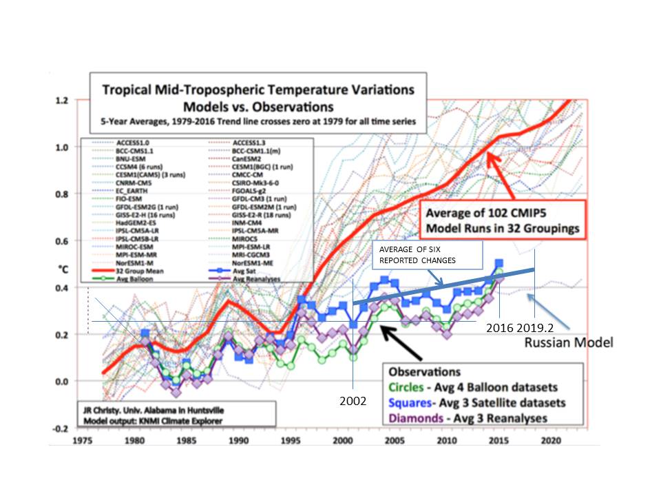 demonstrated that the GCMs are wrong and this paper corroborates that by showing that GCMs have no predictive value. Contribution from CO2, if any, is completely masked by other uncertainties.
Several examples of compelling evidence CO2 has no effect on climate are listed in Section 2 of http://globalclimatedrivers2.blogspot.com . Included also in that analysis is an explanation of WHY CO2 has no significant effect on climate and evidence. Calculations in Section 8 show that water vapor has been increasing about twice as fast as indicated by the temperature increase of the liquid water. The extra increasing water vapor, provided by humanity, has contributed to the rise in average global temperature since the depths of the LIA.
“water vapor has been increasing about twice as fast as indicated by the temperature increase of the liquid water.
That particular forcing is part of the standard global warming theory, atmospheric CO2 changing the energy budget over the decades, warming the oceans and creating these kinds of massive feedback.
The main challenge would be to provide a better theoretical basis for the origin of the increase of water temperature. It’s not clear to me if you’re providing any and yet I’m skeptical of AGW theories too.
JD,
You have been grievously deceived. The water vapor increase resulting from temperature increase is easily calculated from the vapor pressure vs temperature relation. The standard global warming theory assumes that WV increases only as indicated by the temperature increase.
The observation is that, at least since it has been accurately measured worldwide, it has been increasing about TWICE that. Therefore, WV increase is driving temperature increase, not the other way around. Calculations are provided in Section 8 of my blog/analysis http://globalclimatedrivers2.blogspot.com .
I did extensive research into where the extra WV comes from. It is documented in Section 9. The WV increase results mostly (about 86%) from irrigation increase.
NASA/RSS have been measuring water vapor by satellite and reporting it since 1988 at http://www.remss.com/measurements/atmospheric-water-vapor/tpw-1-deg-product . Fig 3 in my b/a is a graph of the NASA/RSS numerical data. When normalized by dividing by the mean, the NASA/RSS data are corroborated by NCEP R1 and NCEP R2.
Pat, in digital simulation , we run min max simulations to ensure our electronic circuitry will run correctly under all expected circumstances. This would, if implemented within climate modelling, mean that each climate run would involve a separate run with each variable at each end of its range. So a million run -4watts, max run +4 watts etc and see that a) the model does not break and b) the error bars are acceptable.
I expect both a) and b) both fail.
Likely, and you put your finger on an important and unappreciated point, Steve.
This is that climate models are engineering models, not physical models.
Their parameters are adjusted to reproduce observables over a calibration period.
A windsteam model for example, is adjusted by experiment to reproduce the behavior of the air stream over an airfoil across its operating specs and some degree of extreme. It can reproduce all needed observables in that calibration bound.
But its reliability at predicting beyond that bound likely diminishes quickly. No engineer would trust an engineering model used beyond its calibration bounds.
But every climate projection is exactly that.
Pat,
Your mention of calibration chimed a memory with me. I was reminded of the Tiljander upside-down calibration issue and so I went looking on Climate Audit. There I found this comment by you dated 17 Oct 2009.
https://climateaudit.org/2009/10/14/upside-side-down-mann-and-the-peerreviewedliterature/#comment-198966
You have been fighting this battle for a long time now.
Duh, This one:-
https://climateaudit.org/2009/10/14/upside-side-down-mann-and-the-peerreviewedliterature/#comment-198987
Extrapolating beyond calibration end-points for a high-order polynomial fit is commonly recognized to be highly unreliable.
Pat, thank you for your careful analysis of my comments further upthread. I am repeating them here annotated with #, and then replying to them.
#See – Owe to Rich, first, you appear to be confusing physical error with uncertainty.
Well, future uncertainty represents a range of plausible physical errors which will occur when that time arrives. So I think it’s just semantics, but let’s not dwell on it.
# Second, I do not “ show that errors in TCF (Total Cloud Fraction) are correlated with latitude” rather I show that TCF errors are pair-wise correlated between GCMs.
Well, Figure 4 shows to they eye that those errors are correlated with latitude, but if that isn’t what you actually analyzed then fair enough. In your “structure of CMIP5 TCF error” you didn’t specify what the x_i were, and I mistook them for latitude rather than a model run.
#Third and fourth, I do not “derive, using work of others, a TCF error per year of 4Wm^-2”.
The ±4W/m^2 is average annual long wave cloud forcing (LWCF) calibration error statistic. It comes from TCF error, but is not the TCF error metric. The LWCF error statistic comes from Lauer and Hamilton. I did not derive it.
OK, semantics again, but they can become important, so I’ll use “LWCF calibration error” from now on.
#Fifth, eqn. 4 does not involve any lag-1 component. It just gives the standard equation for error propagation. As the ±4W/m^2 is an average calibration statistic derived from the cloud simulation error of 27 GCMs, it’s not clear at all that there is a covariance term to propagate. It represents the average uncertainty produced by model theory-error. How does a 27-GCM average of theory-error co-vary?
OK, but the x_i’s here are time, are they not, as we are talking about time propagation? So where x_i and x_{i+1} occur together it is not unreasonable to refer to this as a lag, again it is semantics. And across time intervals, covariation is highly likely.
# Sixth, your “ n years the error will be 4sqrt(n) Wm^-2.” the unnumbered equation again lays out the general rule for error propagation in more usable terms. The u_a … in that equation are general, and do not represent W/m^2. You show a very fundamental mistaken understanding there.
Well, your use of the u_a’s certainly does have some dimension, which I took to be W/m^2, but I now see that it is Kelvin as you talk about “air temperature projections”.
# Seventh, your, “after 81 years that would give 36 Wm^-2,” nowhere do I propagate W/m^2. Equations 5 and 6 should have made it clear to you that I propagate the derived uncertainty in temperature.
Yes, OK, in 5.1 you do convert from the 4W/m^2 into u_i in Kelvins via a linear relationship. It is however true that if we remained in W/m^2 we would indeed reach 36W/m^2 after 81 years. But I’m happy to convert to K first.
# Eighth, your “So I do now see how your resulting large error bounds are obtained. ” It’s very clear that you do not. You’ll notice, for example that nowhere does a sensitivity of 2K or of anything else enter anywhere into my uncertainty analysis. Your need to convert W/m^2 to temperature using a sensitivity number fully separates my work from your understanding of it.
No, really, I do. Whatever units we are working in, an uncertainty E has become, after 81 years, 9E. And actually, though you don’t realize it, you do have an implicit sensitivity number. It is 33*f_CO2*D/F_o = 33*0.42*3.7/33.3 = 1.54K. Here D is the radiative forcing from a doubling of CO2, which IPCC says is 3.7W/m^2, and the other figures are from your paper.
# Ninth, your subsequent analysis in terms of error (“So one flaw … greater flaw as I see it is that global warming is not wholly a cumulative process….) shows that you’ve completely missed the point that the propagation is in terms of uncertainty. The actual physical error is completely unknown in a futures projection.
Semantics again.
# Tenth, your, “hence suffer less error than you predict.” I don’t predict error. You’ve failed to understand anything of the analysis.
I think I’ve understood a lot, thanks.
#Eleventh “Apparently your peer reviewers didn’t spot that point.” because it’s not there. It’s wrong, it exists in your head, and it’s nowhere else.
Yes, that was a bit snarky of me. But I don’t think your use of the error propagation mathematics is correct. Of these eleven points, the fifth one is the only one which really matters and is at the heart of my criticism. I need to go away and do a bit of mathematics to see if I can substantiate that, but ignoring covariance is, I think, the key to the problem. This is certainly interesting stuff.
See, you wrote, “Well, future uncertainty represents a range of plausible physical errors…”
No, it does not. You may dismiss the distinction as semantics, but the difference between error and uncertainty is in fact central to understanding the argument.
You wrote”you didn’t specify what the x_i were, and I mistook them for latitude rather than a model run.”
Here’s how I described the x_i: “For a data series, x_1, x_2,. . . , x_n, a test for lag-1 autocorrelation plots every point x_i against point x_i_1.”
That looks live a very specific description of the x_i to me. And it describes neither a latitude nor a model run.
You wrote regarding the error statistic coming from Lauer and Hamilton, , “OK, semantics again…” That’s the second of your important mistakes you’ve dismissed as mere semantics. How convenient for you.
You wrote, “OK, but the x_i’s here are time …” No, they’re latitude. Look at Figure 5, where the lag-1 plot is shown.
You wrote, “but I now see that it is Kelvin as you talk about “air temperature projections”. The unnumbered equation has no units. It’s a generalized equation. It’s not Kelvins.
You say that “The actual physical error is completely unknown in a futures projection.” is “semantics again. Incredible. It’s mere semantics that physical error is unknown in a futures projection.
Our complete ignorance of the size of the error is why we take recourse to uncertainty.
It’s quite clear that your understanding of the argument in the paper is sorely deficient, See.
Pat, a mathematical equation to describe what you are doing is, I think,
T_i(t) = T_i(t-1) + d_i(t) + e_i(t)
where i is the model number, T_i(t) is temperature at time (year) t, d_i(t) is a non-stochastic increment, and e_i(t) is an error. Then let T(t) = sum_{i=1}^n T_i(t)/n. I don’t accept this as a good summary of the GCMs, but let’s see what it implies. Assume that T_i(t-1) is uncorrelated with e_i(t), and that e_i(t) is uncorrelated with e_j(t) for i!=j. Then
Var[T(t)] = Var[T(t-1)] + sum_i Var[e_i(t)]/n^2 (*)
Now it is possible that e_i(t) to have a structure like e_i(t) = (i-(n+1)/2)a(t) + b_i(t) where a(t) is non-stochastic and b_i(t) has very small variance. In this case Var[e_i(t)] = Var[b_i(t)] in (*) above, and the growth of Var[T(t)] against t is then very small.
Can you prove that something like this is not the case? (I haven’t read the SI to see whether this is covered.) It would be saying that each model i has a bias regarding TCF which does not vary much from year to year. That seems plausible to me, but some torturing of data should reveal the truth.
Look at the figures in Lauer and Hamilton, 2013, See. The model errors are not offset biases.
Your equation is not what I’m doing. The physical errors in projected temperatures are not known.
Annually projected temperature changes are calculated from annual changes in forcing. Their value has no dependence on the magnitude of prior temperature.
Also, uncertainties are not errors. Why is that distinction so invisible to you?
Dr Frank,
I read your paper.
I read the SI.
I watched the video of Dr Patrick Brown.
I read through your exchange of comments with Dr Patrick Brown.
On balance, I am unconvinced by your paper, even though I can list the multiple reasons why AOGCMs have little useful predictive ability.
I have a major concern with your use of a memoryless model to emulate the GCMs, although the problems arising from this are swamped by the larger question of whether it is legitimate to accumulate uncertainty in forcing, and hence temperature, by adding independent samples year-on-year from a distribution with a standard deviation of 4W/m2, as derived from your “global annual cloud simulation calibration error statistic”. In the derivation of this latter statistic, you make no attempt to distinguish between systemic bias and other sources of difference. This is fatal. The distinction is critical to your subsequent uncertainty estimation, and it needs to be founded on individual within-model distinction, before any between-model aggregation or averaging.
To illustrate the point, let us say hypothetically that there is exactly a fixed difference of X in cloud-cover units between every “observed point” and every modeled point (binned at whatever temporal interval you choose), used to derive your calibration data.
Your analysis would translate this difference, X, into a non-zero year-on-year forcing uncertainty of plus or minus Y W/m2. Let us say Y = 4 W/m2 for convenience in this hypothetical example.
Your uncertainty analysis would then yield exactly the same final uncertainty envelope that you display, if I have understood your approach.
However, in the corresponding AOGCM model, while this type of systemic difference in cloud cover is certainly a source of error, the uncertainty in temperature projection which it introduces FROM FORCING UNCERTAINTY is close to zero. (It does introduce a different uncertainty related to the sensitivity of the system to a given forcing, which is quite different, and which most certainly cannot be estimated via adding independent forcing uncertainties in quadrature year-by-year.)
Every AOGCM by prescription produces Pre-Industrial Control runs (“PI control”) for upto 500 years. When a modeling group initiates a run like a 1% per year quadrupling of CO2 or a 20th Century Historical run, the kick-off start-times for multiple runs are selected from time-points towards the end of these runs to allow some variation in initial conditions. The temperature CHANGES and net flux CHANGES from the start-year for each run are then estimated by taking the difference between the run values and the PI Control values at the kick-off point for that run. The temperature and net flux values are then averaged across the multiple runs to produce the data which, for example, you have used in your emulator comparison tests.
The point is that any net flux error arising from a systemic error in cloud cover is already present at the start of the AOGCM run, at which point the system is very close to a net flux balance. All forcing drivers applied thereafter are being applied to a system close to a net flux balance. The systemic cloud error therefore has zero effect on subsequent forcing uncertainty. Since, however, the net flux balance itself is likely to be spurious because of the need for compensation of the systemic error in cloud cover, the sensitivity of the system is probably affected; but this is a different type of uncertainty, with a very different form and propagation characteristics, from the forcing uncertainty which you are purporting to estimate.
Somewhat ironically, one of the arguments used for the comparison of cloud cover averages over different time intervals was that the modeled values were changing slowly. Your paper would be a lot more convincing if you could show in analysis of the cloud cover data that you were specifically attempting to eliminate any systemic difference, since its contribution to forcing uncertainty should be close to zero.
kribaez, that is very interesting. I think you are reinforcing the concerns I have stated above. Your “systemic error in cloud cover” sounds (after converting from W/m^2 to K) like my example (i-(n+1)/2)a(t), where a(t) is non-stochastic and the mean over the n models is zero. Then with “the modeled values were changing slowly” we get b_i(t) with small variance, and it is these small variances (divided by n^2) which can be added to provide the variance growth in projection uncertainty over time.
Does that make sense to you?
The key in Frank’s error propagation is recursive model calculations of everything. I’m not at all sure that GCMs actually do that.
See,
I suspect your n^2 should be n, but yes something like that. My main point was restated by Roy Spencer who must have read my post before commenting (sarc). The forcing value which appears in Pat Frank’s emulator is by definition an induced change in NET FLUX at TOA (or sometimes defined at the top of the climatological troposphere). Any constant offset error in LW cloud forcing is already neutralised by a combination of valid offset (covarying SW) and by compensating errors before any of the AOGCMs start a run. We may not know where the compensating errors are but we know they are there because the TOA net flux is (always) close to being in balance at the start of the run. Such a constant offset difference in LCF between model and reality clearly introduces both error and uncertainty, but by no stretch of the imagination can it be treated as though it were a calibration error in forcing, which is what Dr Frank is doing.
±4W/m^2 is not a constant offset, kribaez.
Nor is it an induced change in net forcing. It is the uncertainty in simulated tropospheric thermal energy flux resulting from simulation error in total cloud fraction.
None of you people seem to understand the meaning or impact of a calibration experiment or of its result.
Dr Frank,
For someone who complains so often about the reading skills and knowledge base of others, you might look to the beam in your own eye. What I invited you to consider was that if there existed such a hypothetical systemic offset, your calibration exercise would include such an offset as part of your estimated forcing uncertainty, despite the fact that it is a completely different animal and absolutely cannot be sensibly propagated as you propagate your forcing uncertainty.
I’ll just quote this one line, because it encapsulates the core of your argument, kribaez: “The point is that any net flux error arising from a systemic error in cloud cover is already present at the start of the AOGCM run, at which point the system is very close to a net flux balance.”
And your equilibrated climate has the wrong energy-state. We know that because the deployed physical theory is incomplete, at the least, or just wrong. Or both.
You’re claiming that the errors subtract away.
However, your simulated climate is projected as state variables, not as anomalies. That means the initial incorrect climate state is further incorrectly projected.
The errors in simulated climate state C_i+1 will not be identical to the errors in C_i, because the extrapolation of an incorrect theory means that output errors further build upon the input errors.
Subtraction of unknown errors does not lead to perfection. It leads to unknown errors that may even be larger than the errors in the differenced climate state variables.
That’s the horror of systematic errors of unknown magnitude. All of physical science must deal with that awful reality, except, apparently, climate modeling.
You say that you read the paper and the SI. This point is covered in detail. Somehow, you must not have seen it.
My emulator comparison tests used the standard IPCC SRES and RCP forcings. And you’ll note that the comparisons were highly accurate.
Also, I estimated no forcing uncertainty. I obtained the LWCF error from Lauer and Hamilton, 2013. What I estimated was a lower limit of reliability of the air temperature projections.
Dr Frank,
“And your equilibrated climate has the wrong energy-state. We know that because the deployed physical theory is incomplete, at the least, or just wrong. Or both.” I agree.
“You’re claiming that the errors subtract away. ” No I am certainly not. I am saying (for the third time, I think) that the errors introduced by a hypothetical constant offset error in cloud coverage do not propagate in the way you have propagated your “forcing uncertainty”, but since you have made no attempt to separate out such error in your calibration, your forcing uncertainty includes and propagates all such error.
“My emulator comparison tests used the standard IPCC SRES and RCP forcings. And you’ll note that the comparisons were highly accurate.” Mmm. I mentioned somewhere above that I was concerned about your use of this emulation model, but decided not to elucidate. I will do so now.
Let me first of all make a statement of the obvious. The forcing term which you use in your emulation equation is a forcing to a net flux, not a net flux. More explicitly, the forcing terms in this equation can be thought of as deterministic inputs (the real inputs are deterministic forcing drivers which are converted by calculation to an instantaneous forcing – an induced or imposed CHANGE in net flux ). These inputs do not include LW cloud forcing; it is NOT an input in this sense. It is one of multiple fluxes which collectively define the climate state in general and the net flux balance in particular. To define the uncertainty in temperature projection, you need to define the uncertainty in net flux (and capacities inter alia).
Your linear relationship describing temperature as a function of forcing can be derived in several ways. One such way is I think important because it starts with a more accurate emulation device than yours, but can be shown to yield your approximation with some simplifying assumptions.
The AOGCMs are known to be close to linear systems in their behaviour. A doubling of a forcing profile results in a doubling of the incremental temperature response profile, and at long timeframes, equilibrium temperature can be expressed as a linear function of the final forcing level. Your model reflects that. More generally, their transient behaviour can be very accurately emulated using an LTI system based on energy balance. For a constant forcing, F, applied at time t = 0, the net flux imbalance N(t) is given exactly by:-
N(t) = Input flux(t) – Output flux(t) = Input flux(0) + F – Output flux(0) – Restorative flux(T,t) (1)
For simplicity, here I will assume a constant linear feedback, γ ΔT, for the restorative flux, although the argument can be extended to cover a more general condition.
Restorative flux (T,t) = γ ΔT where ΔT is the CHANGE in GSAT since t=0.
This yields
N(t) = F – γ ΔT + Input flux (0) – Output flux(0) (2)
If the system starts in steady-state at time t=0, then irrespective of the form of N(t), providing only that it is definable as a linear system in T, we have that T -> F/ γ at long timeframes, since (N ->0). So were does a constant offset error in cloud fraction manifest itself ? It appears here in both the input and output flux at time zero. Let us say that it introduces a net flux error of +4W/m2 downwards. This may be from downward LW or any other cloud-associated flux.
Assuming zero external forcing during the spin-up, Equation 2 becomes
N(t) = 0 – γ ΔT + 4
After 500 years of spin-up, ΔT-> 4/ γ , and the system is a little bit warmer than it was 500 years previously, and it is now back in balance for the start of the 20th century historic run. There is no justification whatsoever for propagating this forwards as though it were the same as a year-on-year uncertainty in forcing or net flux imbalance, which is what you are doing.
There IS justification for describing it as an error and a source of uncertainty, but your treatment of its associated uncertainty seems entirely inappropriate.
kribaez, you wrote, “I am saying (for the third time, I think) that the errors introduced by a hypothetical constant offset error in cloud coverage do not propagate in the way you have propagated your “forcing uncertainty”…”
There is no constant offset error. Take a look at Lauer and Hamilton. All the models show positive and negative error regions.
Those positive and negative errors are combined into a rms global error. That is, ±e. Not +e nor -e.
Confining your analysis to terms of a constant offset error is wrong.
You wrote, “The forcing term which you use in your emulation equation is a forcing to a net flux, not a net flux.
The forcing enters the net flux. The simulation uncertainty — the calibration error — in the net flux establishes the limit of resolution of the model.
That resolution limit is a bound on the accuracy of any simulation. It propagates into sequential calculations. The uncertainty grows with each step. You can’t get around it.
I wonder if some colleagues at SLAC, and elsewhere, would apply this thorough analysis to fusion plasma, likely one of the most difficult areas.
I shudder to think if the delays are due to such errors.
Could it be the climate crew are making mistakes that are systematic in other areas too?
Dr. Frank: “Nick argues for +4W/m^2 rather than the correct ±4 W/m^2 to give false cover to folks like ATTP who argue that all systematic error is merely a constant offset.”
I actually thought the ‘constant offset’ part of Brown’s presentation was a pretty weak analogy, although admittedly I may be missing something important. To me that approach seems to equate to a one-time error in initial conditions; whereas intuitively an error in LCF seems more to be a boundary issue that would have impact as the model steps through time…which would seem correct that the uncertainty would compound over time in some fashion (in annual chunks, 20 year chunks, or continuously, depending on how the +/- 4 w/m^2 is determined).
“all systematic error is merely a constant offset” Especially true of the adjusters at NOAA, but theirs is an example of a systematic error that propagates continuously, and always in the same direction.
Dr. Spencer has posted an article on the paper.
https://www.drroyspencer.com
I look forward to Pat’s reply to Dr. Spencer.
I just do not have the required knowledge to get at this, but something about the following statement of Dr. Spencer raises some flags:
I have replied to Dr. Spencer, Robert.
As you’ll see, he makes so many fundamental mistakes as to remove any critical force from his comments.
Unfortunately, his site does not support the “±.” So, none of them came through in my reply. I had to add a corrective comment after posting to alert readers to this problem.
And it was good reply.
I sensed a bunch of erroneous thinking there in Roy’s analysis, but, again, I lack the knowledge-skill to express the errors, or even understand them fully.
Nonetheless, I remain convinced of the conclusions reached in your paper, PF. I also feel certain that you will have to go through this many more times, with many more people. I hope you’re up for the ensuing ultra-marathon. (^_^) … I’ll be watching, as it unfolds.
After 6 years, 13 submissions, 30 reviewers I think Dr Frank is the Ultra-Marathoner of climate science.
And Dr Frank’s reply is in the comments.
Dr. Spencer is basing his comments upon the actual model behavior, and is ignoring the uncertainty behind the calculations. It is uncertain how cloud behavior really changes when various physical changes happen. The models might accidentally emulate reality, but the mathematical uncertainty remains, and we don’t know how far the model predictions are from what will really happen.
“Dr. Spencer is basing his comments upon the actual model behavior…”
Of course he is! All error propagation is model-dependent. All uncertainty analysis of any output is dependent on the knowledge-space of inputs, validity of model governing equations AND model-dependent error propagation. You cannot get away from the model. Pat’s own work uses a model when he estimates uncertainty based on an emulator of AOGCM results. Roy Spencer’s comments are suggesting that Pat is incorrectly translating an estimated uncertainty in one particular flux, which has close to a 100% compensatory error in the AOGCM, into a bald propagating uncertainty in the net flux imbalance, which is what Pat does when he attaches this uncertainty to his “forcing”. This is not credible. The AOGCM cannot and does not propagate a flux error arising from cloud fraction error as though it were the same thing as a forcing error. You do not need a degree in statistics to understand this.
Try this grossly oversimplified model. A is all incoming flux prior to any forcing. B is all outgoing flux prior to any forcing. N is the net flux imbalance (which is what actually controls temperature change).
N = A – B + F where F is a forcing to the net flux.
B = A with a correlation of 1.
A has a variance of VAR(A). B has a variance of VAR(B) = VAR(A).
Forcing is a deterministic input:- VAR(F) = 0
Under normal statistical rules:-
Var(N) = Var(A) + Var(B) – 2 COV(AB) = 0
Pat’s model examines only the variance of A, without taking any account the compensating correlated value of B. He is in effect saying Var(N) = Var(A+F) = VAR(A)
This is not kosher. In truth, Pat is not doing quite what this model suggests, but it is close and serves to illustrate the key point that Roy Spencer is making.
Windchaser, “Roy Spencer’s comments are suggesting that Pat is incorrectly translating an estimated uncertainty in one particular flux, which has close to a 100% compensatory error in the AOGCM, into a bald propagating uncertainty in the net flux imbalance, which is what Pat does when he attaches this uncertainty to his “forcing”.”
No, that isn’t what Pat does.
You’re equating an uncertainty with a physical error, Windchaser. Big mistake.
The uncertainty is ±4 W/m^2. How is a ±value compensated? No offsetting error can compensate a ±value. Taking a difference merely goes from plus/minus to minus/plus.
You’re basically making the same mistake Roy is: you’re supposing that a calibration uncertainty statistic is an energy flux error. It’s not. That mistake invalidates your analysis.
You wrote, “The AOGCM cannot and does not propagate a flux error arising from cloud fraction error as though it were the same thing as a forcing error. You do not need a degree in statistics to understand this.”
My paper does not discuss physical flux errors that impact simulations. There is nothing for an AOGCM to propagate in a calibration error statistic. The calibration error statistic is not part of any simulation.
You wrote, “Pat’s model examines only the variance of A…”
No, it does not.
Let’s use your simple model to illustrate what’s actually going on, Windchaser. You neglect certain uncertainties.
Corrected, your incoming is A±a and outgoing is B±b. Forcing F is defined in a scenario and is an assigned value with no uncertainty.
Then the uncertainty in the difference, A±a – B±b, is the combined uncertainty of the values entering the difference: sqrt(a^2+b^2) = ±n.
Following from that, A±a – B±b + F = N±n. Your net flux is N±n. When A = B then N = F, and F inherits the uncertainty in N. Every forcing is F±n.
Now we calculate the resulting air temperature from the change in forcing, F±n. The calculated uncertainty in the temperature change reflects the impact of the forcing uncertainty, ±n, and is T±t.
The simulation goes exactly as before, providing discrete values of T for the assigned values of F. The effect on uncertainty due to the ±n conditioning the assigned forcing F is calculated after the simulation is complete.
Now you simulate a future climate knowing that every single F is conditioned with a ±n.
The first step calculates a T_1, which has an uncertainty of ±t_1 due to ±n. The next step also uses F±n to calculate T_2. That value is (T_2)±t_2.
The temperature change at the end of the two steps is the sum of the changes, T_1+T_2, call it T_II.
The uncertainty in T_II is the root sum square of the uncertainties in the two step-calculation: sqrt[(t_1)^2+(t_2)^2] = ±t_II.
So, after two steps our temperature change is (T_II)±t_II, and ±t_II > ±t_1 and ±t_2.
And so it goes for every step. If ±n is constant with each step, then the ±t at each step is constant. After Q steps, the uncertainty in the projected temperature is sqrt[Q x (±t)^2] = ±t_q, and the final temperature is T_Q±t_q. The ±t_q >>> ±t.
None of that is involved in the simulation.
There is nothing for the AOGCM to compensate.
The simulation goes on as before, with TOA balance, discrete expectation values, and all.
However, the growth of uncertainty means that very quickly, the temperature projection loses any physical meaning because ±t_q rapidly becomes very large.
When ±t_q is very large, the T_Q±t_q has no physical meaning. It tells us nothing about the state of the future climate.
Pat,
I think you are blaming Windchaser for my faults.
“You’re basically making the same mistake Roy is: you’re supposing that a calibration uncertainty statistic is an energy flux error. It’s not. That mistake invalidates your analysis.” I knew that I would eventually end up on this growing list.
Staying with the oversimplified example, you wrote:-
“Then the uncertainty in the difference, A±a – B±b, is the combined uncertainty of the values entering the difference: sqrt(a^2+b^2) = ±n.”
The illustrative example specified a correlation of 1.0 between A and B. They co-vary perfectly by assumption. What you have written is therefore nonsense.
If your value of “a” is independently estimated as a sd or an RMSE from calibration data against A, then what you have written is still total nonsense. The uncertainty in the difference is zero, prescribed by the assumption, and the uncertainty in A cannot propagate, despite the apparent calibration error. The covariance is equal to the variance of A which is equal to the variance of B. The difference is zero and the variance of the difference is zero.
The real problem, of course, does not have a perfect correlation between A and B, however, in the absence of external forcing, A-B must drift with small error around zero in the AOGCMs by virtue of the governing equations on which they are based.
Your analysis, however, does not consider the calibration of A, nor the calibration of B, nor the calibration of A-B. Instead, it considers just one flux component which goes into B, and since the sum of all such components must be equal to B, and A-B is bounded, then we can deduce that any error in net flux introduced by this component is largely offset at start-of-run by errors in the other components, such that A-B remains bounded.
kribaez, you’re right, thanks. It was your comment, not Windchaser’s
Apologies to Windchaser and to you. 🙂
You wrote, “The illustrative example specified a correlation of 1.0 between A and B. They co-vary perfectly by assumption. What you have written is therefore nonsense.”
The illustrative example specified A = B with a correlation of 1. Therefore A-B is always 0.
I added uncertainty limits around A and B to make them real-world, rather than your Platonic, ‘perfect knowledge’ model. Adding uncertainties makes your example a useful illustration of what I actually did.
You wrote, “The uncertainty in the difference is zero, prescribed by the assumption, and the uncertainty in A cannot propagate, despite the apparent calibration error.”
Your assumption presumed perfect knowledge of the magnitudes of A and B. You can assume that, of course, but that makes your example useless and completely unrealistic and inapplicable to illustrate an uncertainty analysis.
In fact, if A and B have uncertainties associated with them, then the uncertainty propagates into their difference as I showed.
In Bizzaro-world where everyone knows everything to perfect accuracy and to infinite precision, your ideas might find application. Everywhere else, no.
You wrote, “The covariance is equal to the variance of A which is equal to the variance of B. The difference is zero and the variance of the difference is zero.”
In Bizzaro-world. Not here, where there are limits to measurement resolution, to knowledge, and to the accuracy of physical description.
Neither you nor anyone else can know A and B to perfection. Even if we had a physical theory that said they do vary in perfect correlation, our knowledge of their magnitudes would include uncertainties. That is, A±a and B±b. Then , A±a – B±b = N±n.
Your insistence on an unrealistic perfection of knowledge is hardly more than self-serving.
You wrote, “any error in net flux introduced by this component is largely offset at start-of-run by errors in the other components, such that A-B remains bounded.”
You’re equating errors with uncertainty again. Offsetting errors do not improve the physical theory. With offsetting errors., you have no idea whether your physical description is correct. You therefore have no idea of the correct physical state of the system.
Even if you happen to get the right answer, it provides no knowledge of the state of the real physical system, nor does it provide any reassurance that the model will produce other correct answers.
It doesn’t matter that A-B is bounded. The uncertainty grows without bound as the ±n propagates into and through a sequential series of calculations.
That means there are huge uncertainties in the physical description of your system that are hidden by offsetting errors.
All offsetting errors compound in quadrature to produce an overall uncertainty in the calculation.
Take a look at sections 7 and 10 in the SI, where I discuss these issues at some length.
A spin-up equilibrated simulated climate C_0 is an incorrect representation of the energy-state of the system.
Model theory-error means that the incorrect base-state climate is further incorrectly simulated. The errors in simulated climate C_1 are not known to be identical to those in base-state simulation C_0.
None of the errors are known in a futures prediction. All one can do is use uncertainty analysis to estimate the reliability of the projection. And the uncertainty grows without bound.
Dr Frank,
Thank you for this last response. I now fear that you may be labouring under a serious conceptual misunderstanding.
I would strongly urge you to re-examine what you wrote in your discussion of the law of propagation of uncertainty:- your Equations S10.1 and S10.2.
When I encountered your Equation S10.2, on first reading your SI, I thought that you had just been sloppy with your qualification of its applicability, since, as written, it is only applicable to strictly independent values of x_i . I found it difficult to believe that the NIST could carry such an aberrant mis-statement for so long, so I returned to the Taylor and Kuyatt reference, and found that it did correctly include the covariance terms, which for some inexplicable reason you had dropped with a note saying:-
“The propagation equation S9.2 (sic) appears identically as the first term in NIST eq. A3”
I am at a complete loss to understand why you dropped the covariance terms, but if you believe, as your above response seems to suggest, that var(A-B) = var(A) + var(B) when A and B covary with a correlation coefficient of 1, then that would explain quite a lot about your rejection of the offset error argument.
It would also explain why you think it is reasonable to accumulate the full variance of your forcing uncertainty statistic without accounting for autocorrelation from year to year.
Can you please reassure me that you do understand that your S10.2 is a mis-statement as it stands?
kribaez, I ignored covariance because the LWCF error is a multi-year, multi-model calibration annual average uncertainty for CMIP5 models.
As a static multi-model multi-year average, it does not covary with anything.
Equations S10.1 and S10.2 are exactly correct.
This illustration might clarify the meaning of the (+/-)4 W/m^2 of uncertainty in annual average LWCF.
The question to be addressed is what accuracy is necessary in simulated cloud fraction to resolve the annual impact of CO2 forcing?
We know from Lauer and Hamilton that the average CMIP5 (+/-)12.1% annual cloud fraction (CF) error produces an annual average (+/-)4 W/m^2 error in long wave cloud forcing (LWCF).
We also know that the annual average increase in CO2 forcing is about 0.035 W/m^2.
Assuming a linear relationship between cloud fraction error and LWCF error, the (+/-)12.1% CF error is proportionately responsible for (+/-)4 W/m^2 annual average LWCF error.
Then one can estimate the level of resolution necessary to reveal the annual average cloud fraction response to CO2 forcing as, (0.035 W/m^2/(+/-)4 W/m^2)*(+/-)12.1% cloud fraction = 0.11% change in cloud fraction.
This indicates that a climate model needs to be able to accurately simulate a 0.11% feedback response in cloud fraction to resolve the annual impact of CO2 emissions on the climate.
That is, the cloud feedback to a 0.035 W/m^2 annual CO2 forcing needs to be known, and able to be simulated, to a resolution of 0.11% in CF in order to know how clouds respond to annual CO2 forcing.
Alternatively, we know the total tropospheric cloud feedback effect is about -25 W/m^2. This is the cumulative influence of 67% global cloud fraction.
The annual tropospheric CO2 forcing is, again, about 0.035 W/m^2. The CF equivalent that produces this feedback energy flux is again linearly estimated as (0.035 W/m^2/25 W/m^2)*67% = 0.094%.
Assuming the linear relations are reasonable, both methods indicate that the model resolution needed to accurately simulate the annual cloud feedback response of the climate, to an annual 0.035 W/m^2 of CO2 forcing, is about 0.1% CF.
To achieve that level of resolution, the model must accurately simulate cloud type, cloud distribution and cloud height, as well as precipitation and tropical thunderstorms.
This analysis illustrates the meaning of the (+/-)4 W/m^2 LWCF error. That error indicates the overall level of ignorance concerning cloud response and feedback.
The CF ignorance is such that tropospheric thermal energy flux is never known to better than (+/-)4 W/m^2. This is true whether forcing from CO2 emissions is present or not.
GCMs cannot simulate cloud response to 0.1% accuracy. It is not possible to simulate how clouds will respond to CO2 forcing.
It is therefore not possible to simulate the effect of CO2 emissions, if any, on air temperature.
As the model steps through the projection, our knowledge of the consequent global CF steadily diminishes because a GCM cannot simulate the global cloud response to CO2 forcing, and thus cloud feedback, at all for any step.
It is true in every step of a simulation. And it means that projection uncertainty compounds because every erroneous intermediate climate state is subjected to further simulation error.
This is why the uncertainty in projected air temperature increases so dramatically. The model is step-by-step walking away from initial value knowledge further and further into ignorance.
On an annual average basis, the uncertainty in CF feedback is (+/-)144 times larger than the perturbation to be resolved.
The CF response is so poorly known, that even the first simulation step enters terra incognita.
I am a simple EE so if I am a little off base here be gentle in your criticisms.
==========================================
Dr. Spencer –>
“Climate Models Do NOT Have Substantial Errors in their TOA Net Energy Flux
If any climate model has as large as a 4 W/m2 bias in top-of-atmosphere (TOA) energy flux, it would cause substantial spurious warming or cooling. None of them do.”
…
“The reason is that the +/-4 W/m2 bias error in LWCF assumed by Dr. Frank is almost exactly cancelled by other biases in the climate models that make up the top-of-atmosphere global radiative balance.”
===============================================
This doesn’t seem to be a proof that there isn’t a 4 W/m2 bias derived from TCF.
It seems more a proof that there is an error, but it is offset by other errors in the models.
In the end, accumulated errors may offset each other which seems to validate the linear basis of his model. Yet it doesn’t disprove that individual errors accumulate.
================================================
Systematic errors do accumulate. I’ve already used an example where if you measure a long distance divided into ten segments, five of 10 cm and 5 of 20 cm, with a device that only measures each segment that the errors accumulate.
If the first segment is measured as 10 cm +/- 1 cm and then added to a measurement of the second element of 20 cm +/- 1 cm the error doesn’t stay +/- 1 cm. The uncertainty of the result is really +/- 2 cm. So you end up with a total of 30 cm +/- 2 cm. After measuring the ten segments you will end up with a measurement of 150 cm +/- 10 cm. Your result will have a large uncertainty of what the actual measurement is.
This is not variance or standard deviation or error of the means. It is uncertainty of what the end result actually is. As long as a model uses one calculation to feed another calculation, the uncertainty will accumulate.
And the uncertainty does accumulate here, too, but not as Pat Frank describes.
Most importantly: the uncertainty does not accumulate through time, without end. Rather, the static uncertainty in W/m2 forcing results in a static uncertainty in Earth temperature.
No, it doesn’t Windchaser, because the uncertainty derives from a model calibration error. It invariably enters every simulation step.
I discuss this in the paper. The uncertainty necessarily propagates forward.
Error is bounded. Uncertainty grows without limit.
In your second comment, you’re confusing error with uncertainty. This is a common mistake among my critics.
You can’t know the error in a futures projection. You’re left only with an uncertainty.
To put it another way: actual uncertainties in forcing result in *convergent* errors in temperature. This works the same in models and in the real world: if you perturb or vary the forcings, you get a finite temperature change in response.
Pat Frank’s model has them result in *divergent* errors. This is unphysical as well as also unrepresentative of model physics.
Isn’t it the climate models that imply divergence, hence that hockey stick ?
Pat is simply pointing out that any model which generates such a hockey stick is doing so because it is diverging exponentially from reality.
In the real world there are negative feedbacks that prevent hockey stick scenarios and those negative feedbacks are wholly missing from the models hence the rapidly developing divergence between reality and the hockey stick.
Pat must be right on purely common sense grounds and all the above attempts to confuse and obfuscate are just chaff blowing in the wind.
As for Roy Spencer I no longer give him much credence because he believes in an isothermal atmosphere developing on a rotating sphere illuminated by a point source of light despite the inevitable density differentials in the horizontal plane which would inevitably lead to convection and a lapse rate slope.
I trust him on his speciality of satellite sensing but not on meteorology.
In accountancy one has the interesting phenomenon of multiple ‘compensating’ errors self cancelling so that one thinks the accounts are correct when they are not.
This is similar.
Many aspects of the climate are currently unquantifiable so multiple potentially inaccurate parameters are inserted into the starting scenario.
That starting scenario is then tuned to match real world observations but it contains all those multiple compensating errors.
Each one of those errors then compounds with the passage of time and the degree of compensating between the various errors may well vary.
The fact is that over time the inaccurate net effect of the errors accumulates faster and faster with rapidly reducing prospects of unravelling the truth.
Climate models are like a set of accounts stuffed to the brim with errors that sometimes offset and sometimes compound each other such that with the passing of time the prospect of unravelling the mess reduces exponentially.
Pat Frank is explaining that in mathematical terms but given the confusion here maybe it is best to simply rely on verbal conceptual imagery to get the point across.
Climate models are currently worthless and dangerous.
This post should stay at the top of WUWT as a first read for newbies to WUWT.
Not all climate modelers get it wrong. R. Pielke , Sr. made a similar point, if slightly less blunt, about model limitations here, here:
https://wattsupwiththat.com/2014/02/07/the-overselling-of-climate-modeling-predictability-on-multi-decadal-time-scales-in-the-2013-ipcc-wg1-report-annex-1-is-not-scientifically-robust/
Climate model projections should be scientific discussion points, not guides for environmental policy.
Sorry for the double “here” My editor(me) failed.
Hey Nick,
And my example above , solar constant. It is a flux, and isn’t quite constant, so people average over periods of time. maybe a year, maybe a solar cycle, whatever. It comes to about 1361 W/m2, whatever period you use. That isn’t 1361 W/m2/year, or W/m2/cycle. It is W/m2.
Que pasa? The same Wikipedia states:
Average annual solar radiation arriving at the top of the Earth’s atmosphere is roughly 1361 W/m^2.
So my understanding is that if there is, say +/-54 W/m^2 uncertainty and this uncertainty is not random but systematic therefore when we do calculation per each year such uncertainty will propagate and accumulate.
Yes, it does accumulate. Integrate a W/m2 uncertainty over time, and you get J/m2. This translates into an expanding uncertainty with regard to energy (Joules) as time goes on, or temperature.
But, the hotter the Earth is, the faster it radiates energy away, and the cooler it is, the slower it radiates energy away. The Stefan-Boltzmann Law acts as a negative feedback on any forcing, and keeps the Earth from just accumulating or losing energy without end. This functionally limits the effects of any new forcing. So the systematic uncertainty in energy flux results in a fixed uncertainty in temperature.
That’s how the physics works out, at least. And you can do Monte Carlo simulations to verify — basically, if you have a physics-based simulation of the climate, even a very primitive one, and you sample forcings within +/- 4W/m2, you’ll find that the results at equilbirium is a range of temperatures. That’s how the uncertainty or perturbation actually propagates through, in both models and real world.
Paramenter:
The Wikipedia description is ill-phrased. Since a Watt is equivalent to one joule per second, an (IMO) more useful expression of the value is ‘roughly 1361 Joules per second per square metre at TOA, when averaged over a year.
“Que pasa? The same Wikipedia states:
Average annual solar radiation arriving at the top of the Earth’s atmosphere is roughly 1361 W/m^2.”
Yes. By annual, they are dealing with the fact that due to elliptical orbit it varies during the year. Because it is periodic, when you say annual, you don’t need to specify a start time.
You could equally take an average over two years. Do you think the answer would be 2722? or 1361?
Hey Nick,
I appreciate that, though Wikipedia wording is not great. How I understand ‘error/time unit’ is that this calibration error can be associated with years as calculations are summarised per year, I believe. So, if a speedometer has systematic error of +10% after one hour drive with a constant speed 20 mph the calculated and actual distance will differ by 2 miles. After another hour by 4 hours. In similar manner I understand Pat argumentation – because calculation of greenhouse gases forcing is summarised yearly yearly uncertainty is also +/- 4 W/m^2/year.
Think you meant “by 4 MILES.”
Interesting article to say the least and possibly the most important.
This approximately translates to 4.7k so therefore all RCP’s included in the models with all temperature rises from between 1.5k to 4.5k are all within the annual average of error.
Roy Spencer coming in, agreeing with Nick Stokes and Ken Rice:
https://www.drroyspencer.com/2019/09/critique-of-propagation-of-error-and-the-reliability-of-global-air-temperature-predictions/#respond
The point is that Dr. Spencer already said this error is offset by other adjustments. Two wrongs don’t make a right. If this error was not offset, what would the uncertainty be? Better yet, how accurate are the predictions when multiple errors are used in calculations?
Plus or minus 4 watts per square meter is not a bias; it is a range of values (errors) extending out to plus and minus 4 from the actual illumination for the time of interest, no ?
Yes 🙂
A concept Nick Stokes repeatedly fails to grasp. And, now, apparently, Dr. Spencer.
I’ll reply to his reply, later this evening.
See my replies on Roy’s blog, Windchasers.
Roy has completely misunderstood the paper. He does not understand error analysis at all.
He thinks an uncertainty in temperature is a physical temperature, and he has dismissed as semantics the difference between energy and a statistic.
Roy is a great guy, but he is really far off the mark.
Nick Stokes thinks that instruments have perfect accuracy and infinite precision. See here and posts following.
That’s how qualified he is to criticize science.
Pat,
To underline your point re the accuracy of instruments, here is one example of how our instrumentation is not exactly what some people think it is.
This is one of my Twitter posts from a few months back, and it shows a graph of the various satellites which have measured TSI over the years.
Each device can give a coherent measurement of changes, but there is little agreement from one device to the next.
I think I have a more up to date graph, but this one gives an idea of the issue…they vary from each other by well over 4 watts/meter squared:
https://twitter.com/NickMcGinley1/status/1142820194781450243?s=20
Good example, Nicholas.
A really striking one, though, is an analytical chemistry paper I once found for Geoff Sherrington.
When the Apollo astronauts brought back moon rock samples, it became very important to determine their mineral and elemental content.
NASA folks were very careful. They sent identical rock samples to several different analytical labs. In the event, as I recall, not one lab reported results even within the uncertainty bounds of results from other labs. It was a revelation about the reality of experimental difficulty.
If Geoff is reading here still, he’ll remember the results better than I.
I have that paper somewhere still.
Pat
I have previously remarked that it is my experience that mathematicians tend to be cavalier about precision and units. I suspect that is true because academics are primarily concerned with teaching mathematical theory and technique, and in doing so, rely a lot on exact integers and unitless numbers with infinite precision and perfect accuracy. I learned more about units and precision in my surveying and chemistry classes than I ever did in my mathematics and physics classes.
I agree, Clyde. Mathematicians live in a kind of Platonic utopia. They focus their attention on problems with closed solutions.
Messy problems are annoyances. One of the real problems in climate modeling is that most of the modelers have degrees in applied or other mathematics.
They seem to have no concept of how to deal with real data, or how messy is physical reality.
When dealing with real data, sometimes ad hoc analytical methods must be developed to get a measure of what one has.
I’m reminded of this quote from Einstein, which really fits the bill: “The reciprocal relationship of epistemology and science is of noteworthy kind. They are dependent upon each other.
Epistemology without contact with science becomes an empty scheme. Science without epistemology is – insofar as it is thinkable at all – primitive and muddled.
However, no sooner has the epistemologist, who is seeking a clear system, fought his way through to such a system, than he is inclined to interpret the thought-content of science in the sense of his system and to reject whatever does not fit into his system.
The scientist, however, cannot afford to carry his striving for epistemological systematic that far. He accepts gratefully the epistemological conceptual analysis; but the external conditions, which are set for him by the facts of experience, do not permit him to let himself be too much restricted in the construction of his conceptual world by the adherence to an epistemological system.
He therefore must appear to the systematic epistemologist as a type of unscrupulous opportunist: he appears as realist insofar as he seeks to describe a world independent of the acts of perception; as idealist insofar as he looks upon the concepts and theories as the free inventions of the human spirit (not logically derivable from what is empirically given); as positivist insofar as he considers his concepts and theories justified only to the extent to which they furnish a logical representation of relations among sensory experiences.
He may even appear as Platonist or Pythagorean insofar as he considers the viewpoint of logical simplicity as an indispensable and effective tool of his research.”
Climate modelers as mathematicians are mostly in the epistemologist camp.