26 October 2020
by Pat Frank
This essay extends the previously published evaluation of CMIP5 climate models to the predictive and physical reliability of CMIP6 global average air temperature projections.
Before proceeding, a heartfelt thank-you to Anthony and Charles the Moderator for providing such an excellent forum for the open communication of ideas, and for publishing my work. Having a voice is so very important. Especially these days when so many work to silence it.
I’ve previously posted about the predictive reliability of climate models on Watts Up With That (WUWT), here, here, here, and here. Those preferring a video presentation of the work can find it here. Full transparency requires noting Dr. Patrick Brown’s (now Prof. Brown at San Jose State University) video critique posted here, which was rebutted in the comments section below that video starting here.
Those reading through those comments will see that Dr. Brown displays no evident training in physical error analysis. He made the same freshman-level mistakes common to climate modelers, which are discussed in some detail here and here.
In our debate Dr. Brown was very civil and polite. He came across as a nice guy, and well-meaning. But in leaving him with no way to evaluate the accuracy and quality of data, his teachers and mentors betrayed him.
Lack of training in the evaluation of data quality is apparently an educational lacuna of most, if not all, AGW consensus climate scientists. They find no meaning in the critically central distinction between precision and accuracy. There can be no possible progress in science at all, when workers are not trained to critically evaluate the quality of their own data.
The best overall description of climate model errors is still Willie Soon, et al., 2001 Modeling climatic effects of anthropogenic carbon dioxide emissions: unknowns and uncertainties. Pretty much all the described simulation errors and short-coming remain true today.
Jerry Browning recently published some rigorous mathematical physics that exposes at their source the simulation errors Willie et al., described. He showed that the incorrectly formulated physical theory in climate models produces discontinuous heating/cooling terms that induce an “orders of magnitude” reduction in simulation accuracy.
These discontinuities would cause climate simulations to rapidly diverge, except that climate modelers suppress them with a hyper-viscous (molasses) atmosphere. Jerry’s paper provides the way out. Nevertheless, discontinuities and molasses atmospheres remain features in the new improved CMIP6 models.
In the 2013 Fifth Assessment Report (5AR), the IPCC used CMIP5 models to predict the future of global air temperatures. The up-coming 6AR will employ the up-graded CMIP6 models to forecast the thermal future awaiting us, should we continue to use fossil fuels.
CMIP6 cloud error and detection limits: Figure 1 compares the CMIP6-simulated global average annual cloud fraction with the measured cloud fraction, and displays their difference, between 65 degrees north and south latitude. The average annual root-mean-squared (rms) cloud fraction error is ±7.0%.
This error calibrates the average accuracy of CMIP6 models versus a known cloud fraction observable. Average annual CMIP5 cloud fraction rms error over the same latitudinal range is ±9.6%, indicating a CMIP6 27% improvement. Nonetheless, CMIP6 models still make significant simulation errors in global cloud fraction.

Figure 1 lines: red, MODIS + ISCCP2 annual average measured cloud fraction; blue, CMIP6 simulation (9 model average); green, (measured minus CMIP6) annual average calibration error (latitudinal rms error = ±7.0%).
The analysis to follow is a straight-forward extension to CMIP6 models, of the previous propagation of error applied to the air temperature projections of CMIP5 climate models.
Errors in simulating global cloud fraction produce downstream errors in the long-wave cloud forcing (LWCF) of the simulated climate. LWCF is a source of thermal energy flux in the troposphere.
Tropospheric thermal energy flux is the determinant of tropospheric air temperature. Simulation errors in LWCF produce uncertainties in the thermal flux of the simulated troposphere. These in turn inject uncertainty into projected air temperatures.
For further discussion, see here — Figure 2 and the surrounding text. The propagation of error paper linked above also provides an extensive discussion of this point.
The global annual average long-wave top-of-the-atmosphere (TOA) LWCF rms calibration error of CMIP6 models is ±2.7 Wm⁻² (28 model average obtained from Figure 18 here).
I was able to check the validity of that number, because the same source also provided the average annual LWCF error for the 27 CMIP5 models evaluated by Lauer and Hamilton. The Lauer and Hamilton CMIP5 rms annual average LWCF error is ±4 Wm⁻². Independent re-determination gave ±3.9 Wm⁻²; the same within round-off error.
The small matter of resolution: In comparison with CMIP6 LWCF calibration error (±2.7 Wm⁻²), the annual average increase in CO2 forcing between 1979 and 2015, data available from the EPA, is 0.025 Wm⁻². The annual average increase in the sum of all the forcings for all major GHGs over 1979-2015 is 0.035 Wm⁻².
So, the annual average CMIP6 LWCF calibration error (±2.7 Wm⁻²) is ±108 times larger than the annual average increase in forcing from CO2 emissions alone, and ±77 times larger than the annual average increase in forcing from all GHG emissions.
That is, a lower limit of CMIP6 resolution is ±77 times larger than the perturbation to be detected. This is a bit of an improvement over CMIP5 models, which exhibited a lower limit resolution ±114 times too large.
Analytical rigor typically requires the instrumental detection limit (resolution) to be 10 times smaller than the expected measurement magnitude. So, to fully detect a signal from CO2 or GHG emissions, current climate models will have to improve their resolution by nearly 1000-fold.
Another way to put the case is that CMIP6 climate models cannot possibly detect the impact, if any, of CO2 emissions or of GHG emissions on the terrestrial climate or on global air temperature.
This fact is destined to be ignored in the consensus climatology community.
Emulation validity: Papalexiou et al., 2020 observed that, the “credibility of climate projections is typically defined by how accurately climate models represent the historical variability and trends.” Figure 2 shows how well the linear equation previously used to emulate CMIP5 air temperature projections, reproduces GISS Temp anomalies.

Figure 2 lines: blue, GISS Temp 1880-2019 Land plus SST air temperature anomalies; red, emulation using only the Meinshausen RCP forcings for CO2+N2O+CH4+volcanic eruptions.
The emulation passes through the middle of the trend, and is especially good in the post-1950 region where air temperatures are purportedly driven by greenhouse gas (GHG) emissions. The non-linear temperature drops due to volcanic aerosols are successfully reproduced at 1902 (Mt. Pelée), 1963 (Mt. Agung), 1982 (El Chichón), and 1991 (Mt. Pinatubo). We can proceed, having demonstrated credibility to the published standard.
CMIP6 World: The new CMIP6 projections have new scenarios, the Shared Socioeconomic Pathways (SSPs).
These scenarios combine the Representative Concentration Pathways (RCPs) of the 5AR, with “quantitative and qualitative elements, based on worlds with various levels of challenges to mitigation and adaptation [with] new scenario storylines [that include] quantifications of associated population and income development … for use by the climate change research community.“
Increasingly developed descriptions of those storylines are available here, here, and here.
Emulation of CMIP6 air temperature projections below follows the identical method detailed in the propagation of error paper linked above.
The analysis here focuses on projections made using the CMIP6 IMAGE 3.0 earth system model. IMAGE 3.0 was constructed to incorporate all the extended information provided in the new SSPs. The IMAGE 3.0 simulations were chosen merely as a matter of convenience. The paper published in 2020 by van Vuulen, et al conveniently included both the SSP forcings and the resulting air temperature projections in its Figure 11. The published data were converted to points using DigitizeIt, a tool that has served me well.
Here’s a short descriptive quote for IMAGE 3.0: “IMAGE is an integrated assessment model framework that simulates global and regional environmental consequences of changes in human activities. The model is a simulation model, i.e. changes in model variables are calculated on the basis of the information from the previous time-step.
“[IMAGE simulations are driven by] two main systems: 1) the human or socio-economic system that describes the long-term development of human activities relevant for sustainable development; and 2) the earth system that describes changes in natural systems, such as the carbon and hydrological cycle and climate. The two systems are linked through emissions, land-use, climate feedbacks and potential human policy responses. (my bold)”
On Error-ridden Iterations: The sentence bolded above describes the step-wise simulation of a climate, in which each prior simulated climate state in the iterative calculation provides the initial conditions for subsequent climate state simulation, up through to the final simulated state. Simulation as a stepwise iteration is standard.
When the physical theory used in the simulation is wrong or incomplete, each new iterative initial state transmits its error into the subsequent state. Each subsequent state is then additionally subject to further-induced error from the operation of the incorrect physical theory on the error-ridden initial state.
Critically, and as a consequence of the step-wise iteration, systematic errors in each intermediate climate state are propagated into each subsequent climate state. The uncertainties from systematic errors then propagate forward through the simulation as the root-sum-square (rss).
Pertinently here, Jerry Browning’s paper analytically and rigorously demonstrated that climate models deploy an incorrect physical theory. Figure 1 above shows that one of the consequences is error in simulated cloud fraction.
In a projection of future climate states, the simulation physical errors are unknown because future observables are unavailable for comparison.
However, rss propagation of known model calibration error through the iterated steps produces a reliability statistic, by which the simulation can be evaluated.
The above summarizes the method used to assess projection reliability in the propagation paper and here: first calibrate the model against known targets, then propagate the calibration error through the iterative steps of a projection as the root-sum-square uncertainty. Repeat this process through to the final step that describes the predicted final future state.
The final root-sum-square (rss) uncertainty indicates the physical reliability of the final result, given that the physically true error in a futures prediction is unknowable.
This method is standard in the physical sciences, when ascertaining the reliability of a calculated or predictive result.
Emulation and Uncertainty: One of the major demonstrations in the error propagation paper was that advanced climate models project air temperature merely as a linear extrapolation of GHG forcing.

Figure 3, panel a: points are the IMAGE 3.0 air temperature projection of, blue, scenario SSP1; and red, scenario SSP3. Full lines are the emulations of the IMAGE 3.0 projections: blue, SSP1 projection, and red, SSP3 projection, made using the linear emulation equation described in the published analysis of CMIP5 models. Panel b is as in panel a, but also showing the expanding 1 s root-sum-square uncertainty envelopes produced when ±2.7 Wm⁻² of annual average LWCF calibration error is propagated through the SSP projections.
In Figure 3a above, the points show the air temperature projections of the SSP1 and SSP3 storylines, produced using the IMAGE 3.0 climate model. The lines in Figure 3a show the emulations of the IMAGE 3.0 projections, made using the linear emulation equation fully described in the error propagation paper (also in a 2008 article in Skeptic Magazine). The emulations are 0.997 (SSP1) or 0.999 (SSP3) correlated with the IMAGE 3.0 projections.
Figure 3b shows what happens when ±2.7 Wm⁻² of annual average LWCF calibration error is propagated through the IMAGE 3.0 SSP1 and SSP3 global air temperature projections.
The uncertainty envelopes are so large that the two SSP scenarios are statistically indistinguishable. It would be impossible to choose either projection or, by extension, any SSP air temperature projection, as more representative of evolving air temperature because any possible change in physically real air temperature is submerged within all the projection uncertainty envelopes.
An Interlude –There be Dragons: I’m going to entertain an aside here to forestall a previous hotly, insistently, and repeatedly asserted misunderstanding. Those uncertainty envelopes in Figure 3b are not physically real air temperatures. Do not entertain that mistaken idea for a second. Drive it from your mind. Squash its stirrings without mercy.
Those uncertainty bars do not imply future climate states 15 C warmer or 10 C cooler. Uncertainty bars describe a width where ignorance reigns. Their message is that projected future air temperatures are somewhere inside the uncertainty width. But no one knows the location. CMIP6 models cannot say anything more definite than that.
Inside those uncertainty bars is Terra Incognita. There be dragons.
For those who insist the uncertainty bars imply actual real physical air temperatures, consider how that thought succeeds against the necessity that a physically real ±C uncertainty requires a simultaneity of hot-and-cold states.
Uncertainty bars are strictly axial. They stand plus and minus on each side of a single (one) data point. To suppose two simultaneous, equal in magnitude but oppositely polarized, physical temperatures standing on a single point of simulated climate is to embrace a physical impossibility.
The idea impossibly requires Earth to occupy hot-house and ice-house global climate states simultaneously. Please, for those few who entertained the idea, put it firmly behind you. Close your eyes to it. Never raise it again.
And Now Back to Our Feature Presentation: The following Table provides selected IMAGE 3.0 SSP1 and SSP3 scenario projection anomalies and their corresponding uncertainties.
Table: IMAGE 3.0 Projected Air Temperatures and Uncertainties for Selected Simulation Years
| Storyline | 1 Year (C) | 10 Years (C) | 50 Years (C) | 90 years (C) |
| SSP1 | 1.0±1.8 | 1.2±4.2 | 2.2±9.0 | 3.0±12.1 |
| SSP3 | 1.0±1.2 | 1.2±4.1 | 2.5±8.9 | 3.9±11.9 |
Not one of those projected temperatures is different from physically meaningless. Not one of them tells us anything physically real about possible future air temperatures.
Several conclusions follow.
First, CMIP6 models, like their antecedents, project air temperatures as a linear extrapolation of forcing.
Second, CMIP6 climate models, like their antecedents, make large scale simulation errors in cloud fraction.
Third, CMIP6 climate models, like their antecedents, produce LWCF errors enormously larger than the tiny annual increase in tropospheric forcing produced by GHG emissions.
Fourth, CMIP6 climate models, like their antecedents, produce uncertainties so large and so immediate that air temperatures cannot be reliably projected even one year out.
Fifth, CMIP6 climate models, like their antecedents, will have to show about 1000-fold improved resolution to reliably detect a CO2 signal.
Sixth, CMIP6 climate models, like their antecedents, produce physically meaningless air temperature projections.
Seventh, CMIP6 climate models, like their antecedents, have no predictive value.
As before, the unavoidable conclusion is that an anthropogenic air temperature signal cannot have been, nor presently can be, evidenced in climate observables.
I’ll finish with an observation made once previously: we now know for certain that all the frenzy about CO₂ and climate was for nothing.
All the anguished adults; all the despairing young people; all the grammar school children frightened to tears and recriminations by lessons about coming doom, and death, and destruction; all the social strife and dislocation. All of it was for nothing.
All the blaming, all the character assassinations, all the damaged careers, all the excess winter fuel-poverty deaths, all the men, women, and children continuing to live with indoor smoke, all the enormous sums diverted, all the blighted landscapes, all the chopped and burned birds and the disrupted bats, all the huge monies transferred from the middle class to rich subsidy-farmers:
All for nothing.
Finally, a page out of Willis Eschenbach’s book (Willis always gets to the core of the issue), — if you take issue with this work in the comments, please quote my actual words.
Great work. Another slam dunk that these models are garbage.
Pat Frank,
Thank you for this essay.
Thanks, Matthew.
Pat Frank
You write well. You have provided a clear, understandable explanation of a core problem with the GCMs. I have to conclude that anyone who doesn’t understand what you have written, doesn’t want to understand it. You can lead a donkey to water, but you can’t make it think.
Thanks, Clyde. Just as I was walking out the door after defending my thesis, a bazillion years ago, I heard Dr. Taube (Nobel Prize winning chemist) say, “Well, at least he writes well.” So, I seem to have that covered. 🙂
The angry retorts do seem a partisan matter, don’t they. Lots of people are committed to the AGW bandwagon, and those who do not understand how to think as a scientist have the huge weight of social approval on their side.
The real conundrum is the subscription of the scientific societies. I’ve concluded that lots of the people who do science are methodological hacks — competent at their work but who have not absorbed the way of science into their general consciousness. That makes them vulnerable to artful pseudoscience.
We even see the APS now embracing Critical Race Theory, which has no objective merit at all. No one who has fully integrated the revolutionary improvement in thinking with which science has gifted us could possibly credit such pseudo-scholarship. Hacks.
Pat
You commented on “methodological hacks.” Like technicians with PhD after their name.
I have a similar story to tell. My MSc thesis was so specialized that my committee suggested that I find someone who was a specialist in the area. I asked Dr. Norm J Page of the USGS (Menlo Park, CA) to serve in that capacity. He also asked a newly minted PhD from Stanford to review my thesis, perhaps for her benefit as much as mine. Some years later I ran into her in the halls while visiting someone at the Menlo facility. We were talking and somehow the topic of my thesis came up. She remarked, “You speak so well, I was surprised at how poorly written your thesis was.” I was so taken back by her candor that I was uncharacteristically speechless. However, as I thought about it, I concluded that the difference was, when I open my mouth, I’m solely responsible for my words. However, my written thesis, somewhat like a camel, was the work of all the members of my committee, all of whom I had to please, and none of whom were really expert in the area. However, I did learn to jump through hoops!
One wonders why they think 6 chimps would do a better job than 5 chimps ! 😉
For the same reason we can’t predict the weather reliably for more than about three days, we can’t predict long-term weather (aka climate) for 80 years. I would like to see whether there is a discernible signal in the atmospheric CO2 this year due to the drop in human-produced CO2. There is reasonable data for CO2 production based on our fossil fuel consumption so any blip or lack thereof would be a good indication of the sensitivity of the system and our actual contribution to it.
Loren wrote, ” I would like to see whether there is a discernible signal in the atmospheric CO2 this year due to the drop in human-produced CO2.”
You should not expect that, because normal, transient fluctuations in natural CO2 fluxes cause large year-to-year variations in the rate of atmospheric CO2 concentration increase. Those fluctuations are considerably larger than the change expected due to the Covid-19 recession.
Consider the measurement record for the last decade. Based on annually averaged CO2 levels measured at Mauna Loa…
In 2010 CO2 level was 389.90 ppmv, an increase of 2.47 ppmv over the previous year.
In 2011 CO2 level was 391.65 ppmv, an increase of 1.75 ppmv over the previous year.
In 2012 CO2 level was 393.85 ppmv, an increase of 2.20 ppmv over the previous year.
In 2013 CO2 level was 396.52 ppmv, an increase of 2.67 ppmv over the previous year.
In 2014 CO2 level was 398.65 ppmv, an increase of 2.13 ppmv over the previous year.
In 2015 CO2 level was 400.83 ppmv, an increase of 2.18 ppmv over the previous year.
In 2016 CO2 level was 404.24 ppmv, an increase of 3.41 ppmv over the previous year.
In 2017 CO2 level was 406.55 ppmv, an increase of 2.31 ppmv over the previous year.
In 2018 CO2 level was 408.52 ppmv, an increase of 1.97 ppmv over the previous year.
In 2019 CO2 level was 411.44 ppmv, an increase of 2.92 ppmv over the previous year.
The average annual increase over that ten year period was 2.401 ppmv. But it varied from as little as +1.75 ppmv to as much as +3.41 ppmv.
Mankind added about 5 ppmv CO2 to the atmosphere last year. The Covid-19 slowdown might reduce CO2 emissions by 5 to 10% this year. Even a 10% reduction would make a difference of only about 0.5 ppmv in atmospheric CO2 concentration.
Loren wrote, “There is reasonable data for CO2 production based on our fossil fuel consumption so any blip or lack thereof would be a good indication of the sensitivity of the system and our actual contribution to it.”
The upward trend in the amount of CO2 in the atmosphere is entirely because we’re adding CO2 to the atmosphere, but nature’s CO2 fluxes create “blips” which are larger than the blip to be expected due to the Covid-19 pandemic.
Dave
You remarked, “Even a 10% reduction would make a difference of only about 0.5 ppmv in atmospheric CO2 concentration.” That would be for the annual effect. However, during the time that the reduction took place — perhaps as much as 18% for about 3 months — the NH CO2 concentration was increasing because the tree-leaf sink had not yet kicked in. Therefore, one should reasonably expect to see a decline in the rate of growth equivalent to the decrease in the anthropogenic CO2 flux. That is easier to observe than the net increase over 12 months.
Clyde wrote, “…one should reasonably expect to see a decline in the rate of growth…”
Perhaps. It’ll be hard to notice it, though. 18% of 1/4 of a year of CO2 emissions is only about 0.225 ppmv.
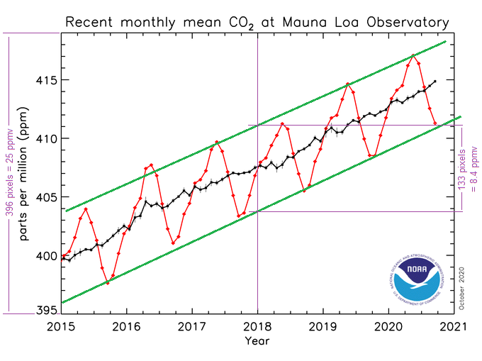
In the northern hemisphere, the seasonal cycle dwarfs that. E.g., at Mauna Loa the seasonal cycle amplitude is about 7 or 8 ppm:
https://www.esrl.noaa.gov/gmd/ccgg/trends/
In the southern hemisphere, the seasonal cycle is much smaller, so a deviation might be easier to see — but the likely Covid-19 slowdown effect is also much smaller in the southern hemisphere.
In any event, it really doesn’t matter whether regulators can measure the results of imposing reduced CO2 emissions, because such changes, even if they have a detectable effect on atmospheric CO2 concentration, would have no real-world benefits. The best evidence is that manmade climate change is modest and benign, and CO2 emissions are beneficial, not harmful.
The only value of such policies is to support the $1.5 trillion/year parasitic climate industry (which, in turn, supports the politicians that prop it up, at everyone else’s expense):
Dave
The change from year to year for a given month is only about 2 or 3 PPM. However, the change from Fall to Spring 2020 is about 8 or 9 PPM, with a distinct peak just before the trees leaf out. If the anthropogenic influence were there, I think we should be able to see it, at least in the slope in the run-up to the peak, and in a reduced peak. That is, there should be a change in shape of the curve from about January to May. It isn’t showing up.
I just took a closer look. At Mauna Loa, the seasonal swing is about 8.4 ppmv, peak-to-peak:
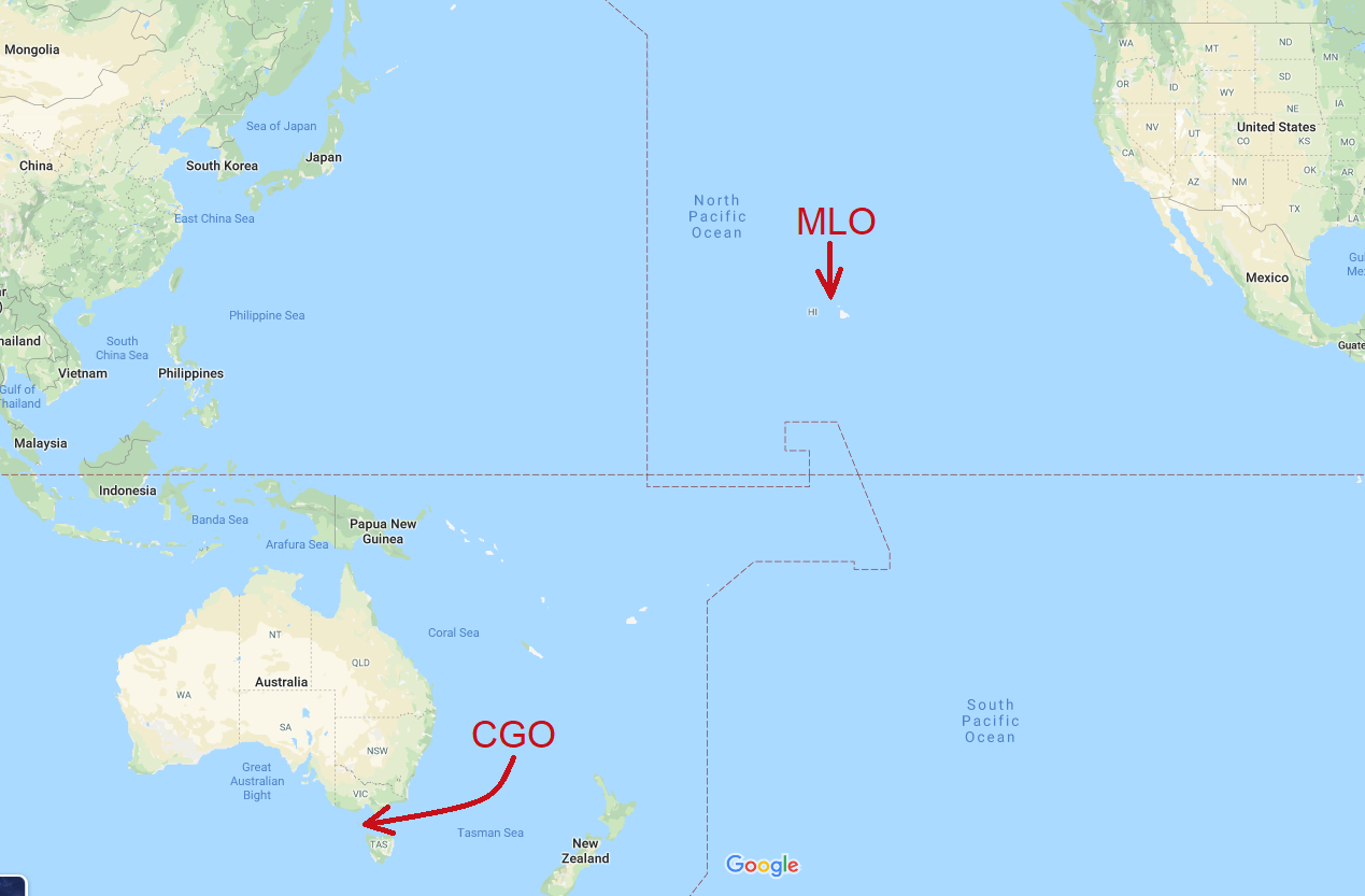
At higher northern latitudes the seasonal swing is larger. At more southern latitudes, it is smaller. At extreme southern latitudes, the seasonal cycle is reversed (but still much weaker):

Here’s a map showing the locations of Mauna Loa and Cape Grim:
I’m not saying that it is impossible to detect a 0.225 ppmv perturbation, but it definitely isn’t easy. I think you’d need to start by trying to remove other, comparable-sized influences, like ENSO.
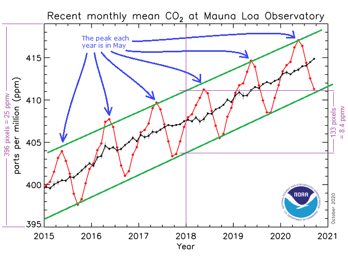
Note: The CO2 seasonal cycle at Mauna Loa peaks in May of each year, which is why, every May/June, like clockwork, we see see a flurry of “news” stories, from the usual propaganda outlets, like The Washington Post and NOAA, about CO2 reaching a record high level.
Dave,
What are the known mechanism that produce these natural variations? Are they adequately quantified?
If an emissions reduction of 10% over 6 months does not make a visible dent, how are regulators going to measure the results of mposing reduced emissions? Ordering another global 10% reduction (were that possible) would increase the risk of armed warfare within and between countries. So the regulators need to get it right. But how will they know?
Geoff S
Geoff, no, the mechanisms are not well understood. They are presumably due to a combination of biological processes, and ocean surface water temperature variations.
There tends to be an uptick in CO2 during El Ninos, e.g., that big 3.41 ppmv jump in 2016.
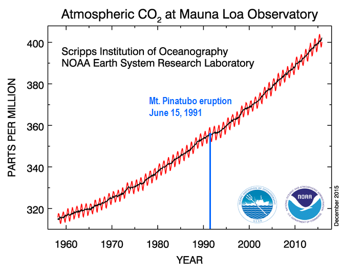
Extremely large volcanoes (esp. Pinetubo!) produce temporary reductions in the rate of CO2 increase, as you can see here:
The effect of El Nino is probably at least partially due to the temperature dependence of Henry’s Law, because an El Nino causes a big patch of warm surface water in the Pacific. However, ENSO cycles have large regional effects on rainfall patterns and fisheries, which could also affect rates of natural CO2 emission and uptake.
The effect from large volcanoes might be due to aerosol/particulate cooling of ocean surface water, and/or perhaps because iron and other minerals in the volcanic ash fertilized the ocean and thereby increased CO2 uptake by ocean biota (Sarmiento, 1993 [pdf]), and/or perhaps because of the effects of sunlight scattering on vegetation growth (Farquhar & Roderick, 2003 [pdf]).
bigoilbob
You wrote above that “FFS, folks, whether you’re whining about normal measurement error or transient, correctable (and mostly corrected) systemic measurement biases, they ALL go away, as a practical matter, when considering regional/world wide changes over climactic physically/statistically significant time periods.”
They do not all go away. You are quite incorrect to assume that and I will give yopu a first-hand example to chew over.
In my younger years I owned an analytical chemistry lab, so my ability to feed my growing family depended on my performance. Performance was advertized by labs like ours and you lost clients if they found you performing worse than advertized. So, we spent a lot of time on concepts and practices of quality control errors of accuracy and precision and uncertainty.
The big show in town at the time was analysis of moon rocks and soils from programs like Apollo 11. A few dozen labs were initially chosen to receive small lots of this expensive material. They were selected on reputation and esteem. Almost all were from universities or government agencies. Besides, they tended to have the most expensive and hard-to-get equipment, like nuclear reactors to do neutron activation analysis.
When the first results came in, shiock horror, there were quite a few cases where a lab’s result was rather different to another or a group of others, beyond the boundaries of how good its performance claimes were. There were labs making errors of accuracy, one different to the next, beyond their claimed precision or advertised scatter based on repeated analysis of lots of the same material.
These errors do not go away. The reults, in theory, can be made to converge if one or more – even all – of the labs make adjustments to their methods. These adjustments are hard to design because often you do not know what causes the error and more importantly, nobody knows the “right” answer.
Over the course of time, instruments have improved. Electronics, for example, are far more stable than in the 1970s. Accuracy might have improved overall, one hopes so – but we still have the problem that a lab operating in isolation has no idea of what the right answer is. Such labs cannot improve their accuracy by doing multiple analysis of a constant material.
Coming back to GCMs and their problems, none of them knows what the right answer is. Some answers can get accepted as ok to work with when critics can find no objections to the methods and their execution. In other cases, to gain a continued living, modellers can converge on some critical values through a consent like process that might run in the mind like “All the other guys are getting a value of XYZ, a bit higher than mine. If I wind down this calibration here, mine fall into line and I can add my XYZ to the pool. This is what happens to real humans in real life. Sad, but true. It is not felt to be cheating or anti-science, it is a normal human herd response who consequences can be so trivial that nobody can really object.
All through this business of errors and GCMs, Pat Frank has been correct with his assertions and calculations. Proof is that nobody has shown him to be incorrect. That is not an absolute test, but it is a good one.
Half the time I read “CMIP6” as “Chimps”, and the rest of the time I read it as “Chips”.
Now I’m hungry.
Me too, especially when it was CMIP5.
Thanks Dr Frank, again for taking us carefully through the maze of error v uncertainty; it bells the cat of predicted CATastrophic atmospheric warming;
I also see the statistics urge to deal with randomly distributed readings using a presumption of a normally distributed variable :
I can also see uncertainty in iterative processes is at least additive –
I wonder if there is another good simple analogy that can unlock the ‘hole’ that people put themselves in – Thanks to Jim Gorman for his explanations.
The modelled prediction of warming is not an empirical data point:
I need to say it over and over
In Kansas we have the odd windy day
Thanks, Dorothy.
Models can’t predict what will happen with CO2, if anything. All the data show the behavior of the modern climate is indistinguishable from natural variability.
Everyone should feel comfortable, and just go about the business of their lives.
A later WUWT post seems to show seriously cold weather heading your way. So, see to your battening down. Stay safe and ready your galoshes. 🙂
Most of the comments are in favor. Are you here to cheerlead? A lot other issues are brought up.
The next step is to remove the error that is said to exist.
The next step is to move this theory to other models and tell why they don’t work.
In a simple game, damage done has a bell curve distribution. Who expects to do damage for the whole sequence of the fight only more than 2 standard deviations above the average? Someone that’s going to lose.
Ragnaar, you haven’t read the original paper, have you. It’s not just this one model.
Take a look at Boucher, et al., 2020, Figure 18. All the CMIP6 models make significant long wave cloud forcing (LWCF) simulation errors.
The CMIP6 average annual rms error is ±2.7 W/m^2. And that’s not a base state error. It’s the average annual calibration uncertainty in simulated LWCF across every single year of a simulated climate.
The fact that every model makes a LWCF error of different magnitude, by the way, reveals the variable parameterization sets the models have had installed by hand, so as to tune them to known target observables. The whole effort is a kludge.
If you plot a “Drunk Walk” with a random number between plus & minus 2.7 seeded with zero and 80 iterations (by 2100) it can quickly go off scale. Or is there some tendency toward zero?
The ±2.7 W/m^2 isn’t error, Steve, it’s uncertainty. So there’s no random walk of that number.
The model physics has boundary conditions, so its simulation errors can’t make it run off to infinity. The climate is physically bounded, so it’ll stay within a certain range of states.
One can’t know the errors in a futures projection. But one can know, from the presence of model calibration errors, that simulation errors will cause the predicted climate to do a random walk in the simulation phase space, away from the physically correct solution.
It’s just that the sign and magnitude of the physical errors in the predicted future climate are unknown. So, one needs an alternative reliability metric. That’s where propagation of the calibration error statistic comes into use.
Thanks for the reply – I’ll have to run through it a few times to see if I get the gist of what it is that you are saying. (-:
Why wouldn’t the best case be 10 feet exactly? Not likely, but still possible, ergo the best case.
Dave,
What are the known mechanism that produce these natural variations? Are they adequately quantified?
If an emissions reduction of 10% over 6 months does not make a visible dent, how are regulators going to measure the results of mposing reduced emissions? Ordering another global 10% reduction (were that possible) would increase the risk of armed warfare within and between countries. So the regulators need to get it right. But how will they know?
Geoff S
See https://wattsupwiththat.com/2020/10/27/cmip6-update/#comment-3114145
Pat Frank, thank you for this update. I greatly appreciate that you have so effectively followed a formal analysis from the acknowledged cloud fraction error to its necessary conclusion about uncertainty, and have stayed with that conclusion against such vehement disagreement from those who should know better. I look forward to your analysis of the temperature record. It is worth it to keep pressing on.
Thanks, David. Your encouragement is greatly appreciated, really and truly.
Pat,
Did yu see my comment above how increased model resolution does not help if there is a large continuum error
exactly as you stated.
Jerry
Hi Jerry — yes, I did see it, thanks. And, as usual with your posts, I learned something from it.
One is that I should read your papers more carefully (and probably several times). 🙂
The other is I didn’t realize that the continuum errors in the physical parameterizations that are hidden using hyperviscosity are apparently the major source of model error; at least as regards simulation of short- and medium term atmospheric dynamics.
One question that occurred to me is, if models are repaired along the lines your described, presumably weather forecasting would become more accurate and reliable over longer terms. Is that right?
But how far out do you think climate simulations could go before becoming unreliable? Would the resolution of climate models improve enough to predict the effect of the 0.035 W/m^2 annual perturbation of GHG’s?
Pat,
Although we have now pointed out the correct dynamical equations that must be used, the observational and parameterization errors are so large as to overwhelm an extended weather forecast. It has been demonstrated that inserting perfect large scale data periodically in a standard turbulence model will eventually reproduce the correct smaller scales of motion starting only from the correct large scale initial data.
This is essentially the process the weather forecasters are using when inserting new large scale data every few hours. But they do not have perfect large scale data or forcing (parameterizations).
Your analysis holds for longer term integrations. In a hyperbolic system started with perfect data at time 0 but with a continuum error ( in the equations, forcing, or numerical error) there will be an error in the solution at a later time t1.
Now start the system up at that time and there is an error in the initial data
plus any of the errors mentioned above are still there in the ensuing solution.
There are many examples that the accuracy of numerical solutions compared to a known solution deteriorates over time just from truncation errors in agreement
with your analysis.
Jerry
If I might be so bold as to offer a short quote from Dr. Taylor’s exposition on uncertainty analysis:
“In the basic sciences, error analysis has an even more fundamental role. When any new theory is proposed, it must be tested against older theories by means of one or more experiments for which the new and old theories predict different outcomes. In principle, a researcher simply performs the experiment and lets the outcome decide between the rival theories. In practice, however, the situation is complicated by the inevitable experimental uncertainties. These uncertainties must all be analyzed carefully and their effects reduced until the experiment singles out ne acceptable theory. That is, the experimental results, with their uncertainties, must be consistent with the predictions of one theory and inconsistent with those of all known, reasonable alternatives. Obviously, the success of such a procedure depends critically on the scientist’s understanding of error analysis and ability to convince others of this understanding.”
Since none of the model authors bother to do an uncertainty analysis of the inputs to their models let alone a summary uncertainty analysis of their outputs, how are the models supposed to be separated out to determine one acceptable theory? The wide spread of results from the various models would seem to indicate to an impartial judge that none of them provide a match to actual reality – meaning none of the theories (i.e. models) are acceptable predictors of the future.
The fact that so many climate scientists are un-accepting of uncertainty analysis of an iterative process is a prime indicator that they are themselves unsure of the ability of their models to predict the future. Ranting and raving about “denial” is an emotional argument, not a rational, logical argument.
That quote is on page 7 of my 2nd Edition, Tim, which just arrived yesterday. 🙂
Here’s a quote from page 6, which goes right to the heart of the climate model problem, “Note next that the uncertainty in George’s measurement is so large that his results are of no use.”
CMIP5/CMIP6 air temperature projections in a nutshell.