From Dr. Roy Spencer’s Global Warming Blog
Roy W. Spencer, Ph. D.
The Version 6 global average lower tropospheric temperature (LT) anomaly for March, 2024 was +0.95 deg. C departure from the 1991-2020 mean, up slightly from the February, 2024 anomaly of +0.93 deg. C, and setting a new high monthly anomaly record for the 1979-2024 satellite period.
New high temperature records were also set for the Southern Hemisphere (+0.88 deg. C, exceeding +0.86 deg. C in September, 2023) and the tropics (+1.34 deg. C, exceeding +1.27 deg. C in January, 2024). We are likely seeing the last of the El Nino excess warmth of the upper tropical ocean being transferred to the troposphere.

The linear warming trend since January, 1979 remains at +0.15 C/decade (+0.13 C/decade over the global-averaged oceans, and +0.20 C/decade over global-averaged land).
The following table lists various regional LT departures from the 30-year (1991-2020) average for the last 14 months (record highs are in red):
| YEAR | MO | GLOBE | NHEM. | SHEM. | TROPIC | USA48 | ARCTIC | AUST |
| 2023 | Jan | -0.04 | +0.05 | -0.13 | -0.38 | +0.12 | -0.12 | -0.50 |
| 2023 | Feb | +0.09 | +0.17 | +0.00 | -0.10 | +0.68 | -0.24 | -0.11 |
| 2023 | Mar | +0.20 | +0.24 | +0.17 | -0.13 | -1.43 | +0.17 | +0.40 |
| 2023 | Apr | +0.18 | +0.11 | +0.26 | -0.03 | -0.37 | +0.53 | +0.21 |
| 2023 | May | +0.37 | +0.30 | +0.44 | +0.40 | +0.57 | +0.66 | -0.09 |
| 2023 | June | +0.38 | +0.47 | +0.29 | +0.55 | -0.35 | +0.45 | +0.07 |
| 2023 | July | +0.64 | +0.73 | +0.56 | +0.88 | +0.53 | +0.91 | +1.44 |
| 2023 | Aug | +0.70 | +0.88 | +0.51 | +0.86 | +0.94 | +1.54 | +1.25 |
| 2023 | Sep | +0.90 | +0.94 | +0.86 | +0.93 | +0.40 | +1.13 | +1.17 |
| 2023 | Oct | +0.93 | +1.02 | +0.83 | +1.00 | +0.99 | +0.92 | +0.63 |
| 2023 | Nov | +0.91 | +1.01 | +0.82 | +1.03 | +0.65 | +1.16 | +0.42 |
| 2023 | Dec | +0.83 | +0.93 | +0.73 | +1.08 | +1.26 | +0.26 | +0.85 |
| 2024 | Jan | +0.86 | +1.06 | +0.66 | +1.27 | -0.05 | +0.40 | +1.18 |
| 2024 | Feb | +0.93 | +1.03 | +0.83 | +1.24 | +1.36 | +0.88 | +1.07 |
| 2024 | Mar | +0.95 | +1.02 | +0.88 | +1.34 | +0.23 | +1.10 | +1.29 |
The full UAH Global Temperature Report, along with the LT global gridpoint anomaly image for March, 2024, and a more detailed analysis by John Christy, should be available within the next several days here.
The monthly anomalies for various regions for the four deep layers we monitor from satellites will be available in the next several days:
Lower Troposphere:
http://vortex.nsstc.uah.edu/data/msu/v6.0/tlt/uahncdc_lt_6.0.txt
Mid-Troposphere:
http://vortex.nsstc.uah.edu/data/msu/v6.0/tmt/uahncdc_mt_6.0.txt
Tropopause:
http://vortex.nsstc.uah.edu/data/msu/v6.0/ttp/uahncdc_tp_6.0.txt
Lower Stratosphere:
http://vortex.nsstc.uah.edu/data/msu/v6.0/tls/uahncdc_ls_6.0.txt
I had expected temperatures to start to fall this month. Will be interesting to see how this compares to the surface data sets.
This breaks the old March record, set in 2016 by 0.3C, which in turn was about 0.3C warmer than the other contenders.
Top ten warmest March Anomalies in UAH history, back to 1979 are.
This makes 9 months in a row that have been the record for that month.
So what?
You’ll have to ask this web site why they keep publishing UAH updates every month. If you are not interested in them, you could just ignore them.
It’s not easy to ignore a 0.02 degrees of statistical heating increase. I had to get up early to turn off the furnace each morning in March because it was getting too hot to sleep.
Unfortunately, my thermostat is only programmable in degree units, so its useless to reprogram it. I’ve written Gavin Newsom about the lack of oversight that major Corporations have from the State when designing useful thermostats, but I haven’t heard back.
Yes, as Colonel Kurtz said –
“the horror”
He could have been talking about that 0.02 degrees of blast-furnace heating the planet is experiencing.
And what are the +/- tolerances around your setting? Perhaps 2 or 3 degrees F?
I was asking about the statement you made. I suspect you think that the data to which you refer is alarming and somehow tied to fossil fuel use, but I was giving you the chance to say that, if indeed that was your point.
You know that the bellboy will never be able to show any human causation in these El Nino events.
It has, in fact, many time stated that he purposely doesn’t mention it…
… a tacit admission that it knows these events are totally natural.
You can’t look at a graph of temperatures and deem to know what is causing the observed variability, you need to construct a physical theory to explain the observations. Bellman is not trying to explain why the temperatures are changing in the way that they are, they are simply describing the change.
Why do new temperature records keep getting set? Maybe it’s because El Nino is getting stronger and stronger over time, as you claim, but you have to present your physical theory, backed up by evidence, to convince anyone of this. Why is El Nino getting stronger and stronger? You never can say.
The GAT is a meaningless number that cannot represent “the climate”, yet all you ruler monkeys treat it as such.
The global air temperature anomaly does not represent the climate, it represents a change in the global energy state (i.e. it tells us that the climate is changing).
But, importantly, just seeing a change in the global energy state doesn’t tell you anything about what is causing the change, you only know that a change is occurring. Bnice thinks they know exactly what is causing the change – El Nino getting warmer and warmer over time, but can’t point to any physical theory to actually substantiate that conjecture.
Nice hand-waving, devoid of meaningful content.
“The global air temperature anomaly does not represent the climate, it represents a change in the global energy state (i.e. it tells us that the climate is changing).”
Malarky! The temperature doesn’t determine the energy state. The energy state is a complex functional relationship with numerous factors, such as humidity and pressure. The temperature can change while the energy state remains constant!
You would have us believe that things like pressure and humidity are not relevant factors. So does climate science. That’s why climate science has refused to convert to using enthalpy instead of temperature even though the data to calculate enthalpy has been available for at least some measurement stations for over 40 years!
“You can’t look at a graph of temperatures and deem to know what is causing the observed variability,”
You can’t look at a graph of temperatures and know *anything* about what is actually going on. It is *energy* content that is important and temperature is a piss-poor metric for energy, i.e. enthalpy.
What new temperature records are being set? Max temps? Min temps? Daily mid-range temps? Global anomaly values?
Record temperatures are typically WEATHER related, not climate related. And they are blips on the radar, not indicative of climate change at all. You don’t even have this one right!
And *you* want to talk about someone never saying? When are you going to give us the variances of the temperature data for ONE station over a period of time? If you don’t know the variance then you have no metric for determining how accurate the “average” value might be! But you seem to be ok with that since it is *your* failing to elucidate on the subject.
You can look at a graph of global temperatures and tell whether the planet was in an ice age or an interglacial period. Temperature is a useful metric to track. Sometimes it would behoove you to take a step back, inhale, and ask yourself if you’re really making any sense.
Check the mirror you are standing in front of first.
To paraphrase: “The Hypocrisy runs deep in you”. Just a few messages ago you admitted temperature cannot differentiate between different climates. Now you are claiming that temperature *can* differentiate between different climates.
Pick one and stick with it.
Who are you paraphrasing? I said that two places with the same mean climate might exhibit different mean temperatures, so you will need to observe other parameters to determine if they have different climates. I then said that two places might have all other parameters equal (e.g. dry, arid), and you need to observe the mean temperature to know if they have different climates.
This is different than noting that the global mean surface temperature can distinguish between different global climate states like ice ages and interglacials.
Sometimes I hope you’re just playing the fool for laughs, because the possibility that you are genuinely this obtuse is too sad to dwell on for long.
Just stop with the irony, you don’t WTF you yap about.
It’s all he has. There’s nothing as bad as being intentionally ignorant.
And then puffing yourself up as some kind of expert.
Why then do the climate models exhibit such a tight correlation with CO2 while missing the long pauses that occur while CO2 is growing? Why do the models with such a tight correlation with CO2 run too hot?
What parameters are the models missing?
The problem is that temperature is *NOT* the only control knob yet the models pretend that it is and that CO2 is the controlling factor.
CO2 is *not* the only factor and temperature is a piss-poor metric for energy content. Two simple facts which, for some reason, you can’t accept.
Plus the fact that after just a few iterations, these massive climate models become nothing but linear extrapolations of rising CO2 content.
Then he tried to gaslight by claiming the GAT and CO2 aren’t the only parameters the climate pseudoscientists look at.
Climate models model internal variability, but they do not replicate it. That is, random, or quasi-cyclic, fluctuations appear in the models with the correct periodicity and magnitude, but not at the same time as they are occurring in the real world, because the models are, well, models. If you post-hoc force the model with known factors, it will capture the resultant variability (e.g. adding forcing from a volcanic eruption), but the model has no way of knowing that a volcanic eruption is supposed to occur in the future. That’s just a random occurrence that has a short term impact on the long term trend.
Similarly, models produce hurricanes, but they don’t produce the exact set of hurricanes we experience in the real world unless we are feeding them tons and tons of data about the exact conditions occurring at the time of the storm, and even then they don’t give us the exact storm we are observing (that’s why there’s uncertainty in e.g. storm track forecasts).
That is flagrantly wrong, and betrays a deep ignorance of how climate models are built and how they function. I’d again refer you to the intro textbook I linked to.
Is hand-waving all you climate chicken littles have in the tank?
It’s ok to say things like, “I don’t understand what you just wrote, Alan, can you simplify/clarify it for me?” But, again, if you’d go do your reading as I prescribed you wouldn’t be having this struggle right now.
Not going to waste my time reading crap written by compatriots of Jones and Mann who decided they needed to “hide the decline” with fraudulent contortions to historic data.
“Climate models model internal variability, but they do not replicate it. That is, random, or quasi-cyclic, fluctuations appear in the models with the correct periodicity and magnitude, but not at the same time as they are occurring in the real world, because the models are, well, models.”
This is nothing more than saying some models are useful and that the models will be right in the long term. The models are now almost 40 years old and they are getting WORSE, not better, when compared to observations!
” the model has no way of knowing that a volcanic eruption is supposed to occur in the future.”
And yet it is these occurrences that have a large impact on the future! Like I keep saying, you are trying to say that the models *can* predict the future while at the same time saying they can’t! If you don’t know what is going to happen in the future then how do you predict the future?
“Similarly, models produce hurricanes, but they don’t produce the exact set of hurricanes we experience in the real world”
The models say hurricane occurrences are supposed to INCREASE while in the real world they aren’t. That is not just missing an exact match, it is just plain wrong!
Supposedly the models have shown for the last 30 years that food production will crash because of higher temps but for 30 years all we see are continued record food production every year. Same for the Artic ice disappearing, polar bears going extinct, and the oceans boiling. Is there *anything* the models get right? It certaintly isn’t getting the temp right.
“That is flagrantly wrong”
No, it is right. It can be shown by the close correlation of the models predicted temperature rise with the predicted growth of CO2 emissions. If the models had other factors significant factors right you wouldn’t see the close correlation with CO2. It’s why Monckton’s pauses are so important to recognize and understand.
I think they’re doing pretty darn well compared to observations:
No one has ever said models predict the future, in fact scientists are extremely careful to point out that the models do not provide predictions. That’s why the IPCC presents a range of different projections based on various forcing scenarios. What models say is, “if emissions follow this pathway, these are likely outcomes,” for instance. They have no way of knowing which pathway might actually be followed, because that’s a function of human behavior.
CO2 forcing has been the dominant driver of the warming observed over the past 50 or so years, so it’s unsurprising that the models generally show the warming as a function of CO2 forcing. There isn’t any other forcing capable of explaining the observed change:
Monckton’s pauses are completely unimportant, it’s just a dumb thing that people without any understanding of climate dynamics fixate on.
“I think they’re doing pretty darn well compared to observations:”
Bullcrap. Even the IPCC has had to admit the models are running too hot. The only scenario that is even close is one using a CO2 growth rate that is *SMALLER* than what is being seen in reality!
“in fact scientists are extremely careful to point out that the models do not provide predictions.”
Huh? What scientists are you speaking of? Then why so many studies saying that the earth is going to turn into a cinder? Why so many studies predicting a crash in food production due to HIGHER temperatures? Why so many studies predicting a growth in species extinctions due to HIGHER temperatures? And on and on and on and on and on …..
“CO2 forcing has been the dominant driver of the warming observed over the past 50 or so years”
An unproven assumption. It’s religious dogma, nothing more. If it was the DOMINANT driver then we wouldn’t have seen the multi-decadal pauses in temperature rise over the past 30 years since CO2 has continued to grow practically unabated the whole time!
A subset of models in CMIP6 run too hot, that is not “the” models. But even then, observations fall well inside the envelope of CMIP6 projections:
And, as shown above, even Hansen’s earlier projections from 1988 were on the mark.
I don’t know of a single study saying the earth is going to turn into a cinder. Can you cite them? Most projections show temperature rising because most projections involve scenarios with a continuing CO2 increase. Projections involving scenarios with net-zero CO2 or a CO2 drawdown do not show temperatures continuing to rise over the 21st century. This, again, highlights the difference between a prediction and a projection. Prediction: this is how humans are going to behave in the coming years, and this is how the climate will likely change as a result. Projection: this is one possible way humans might behave in the coming years, and if they do, this is how the climate will likely change as a result.
Chew on those for a while and see if you can spot the differences.
A projection is, at its base *is* a prediction. If you don’t assume how humans will behave then you can’t project anything – it all becomes swirls in a cloudy crystal ball.
If you can’t assign a value to a “projection” for how likely it is to happen then it is worthless. The only way to assign such a value is to assume how people will act – the same as for a prediction.
Do you also believe in the “projections” made by carnival fortune teller hucksters?
What a moronic comment !
Something you would expect from a RABID AGW-cult-apostle.
It will take quite a while—years—for Tongan eruption blasted water vapor and sulfate aerosols to settle out of the stratosphere.
https://www.pnas.org/doi/10.1073/pnas.2301994120
Don’t blame me, I was nowhere near that volcano.
I blame the trendologists.
I’m afraid that I will have to confess to seeing something in the entrails of Hunga-Tonga. This was not a typical El Nino event. In 1998 and 2016, the temperature peaked and declined the next month. This time, it seems that there is a convention being held around the 0.9 anomaly, without the usual rapid decline. Things are getting curiouser and curiouser.
NASA has pointed out that the massive volume of water (Tonga) reaching the ozone layer will take 5 years or more to dissipate.
They say that this water:
“…would not be enough to noticeably exacerbate climate change effects.”
The real problem nowadays, is finding enough virgins to tame these volcanoes. !
I’ll be within a few thousand miles in a couple of weeks. Maybe I should keep my eyes peeled.
Tonga no longer keeps its virgins peeled:
Gosh darn it!
Ah so are we one step closer to finding the cause of the eruption? An in-depth investigation of Tongan virgins may be necessary – volunteers please form an orderly queue.
The gods are angry!
The gods must be crazy!
I’d volunteer to save the planet, but…. Hmmm…. Maybe Greta will volunteer? Nah.
I think that the problem started in the ’60s or ’70s.
We know of four factors which have contributed significantly to the recent warmth (and there might be others we don’t know about). The four are:
#1. The unusual 2022 Hunga Tonga volcanic eruption, which humidified the stratosphere, which you mentioned.
#2. The El Niño, of course.
#3. The IMO 2020 pollution controls on ships. They resulted in “an estimated 46% decrease in ship-emitted aerosols.” Because ships are a major contributor, that caused a sharp 10% decrease in total global sulphur dioxide (SO2) emissions.
That’s a large reduction in air pollution in a very short time. Cleaner air reflects less sunshine, which causes you-know-what to become slightly milder.
#4. The slow, steady rise (25 ppmv/decade) in the atmospheric concentration of what Scientific American once called “the precious air fertilizer.”
The rise is generally benign. (It’s extremely helpful to Germany, which managed to get along last winter without Russian natural gas, and probably will be okay this winter, too, thanks to milder than usual winters.)
It is all good news, except that the first 2 of those 4 factors are transient.
Too bad MV Dali didn’t get the clean bunker fuel memo.
Nope – CO2 does nothing other than improve the biosphere.
You missed the most important factor driving the trend. Solar intensity shifting northward. It peaked in the SH 500 years ago. The change in the NH is accelerating slightly typical of a sine wave past its minimum.
The middle chart in the attached shows the UAH trend across latitudes. It has distinctive lobes in the region of the Ferrel Cells in both hemispheres.
Note the ocean heat content peaks at 45S also in the Ferrel Cell. These are net condensing regions as shown by the high negative Net radiation in the region of the Ferrel Cells.
Now explain to me how CO2 is selectively warming in the regions of the Ferrel Cells.
Come on Rick. Don’t be drawn into this ”trend” bullshit. The GAT was more or less the same in 1958 as it was in 2001 and today’s temps (besides this latest peaking) is probably more or less the same as it was just after WW2 there is no ”trend” in the weather because there is no ”trend” in temperatures. Hysterical narratives is the only place we can find a real trend.
The red arrow on the graph below shows the start of the satellite measurements.
There is a well established warming trend; most notably in the NH. The Vikings abandoned Greenland in 1450. The colony failed through climate changing from when they first arrived about 400 years earlier.
Thames frost fairs were a feature from 1600 up to the early 1800s.
The CET has readings dating back to 1659. The first 100 years warmed 0.6C. The second 100 increased but next to nothing. The third 100 to 1959 warmed 0.6C and the last 70 warmed 1.4C. The latter likely influenced by urban development.
Oceans have been steadily rising for at least 200 years through a combination of melting land ice and heat retention.
I am not a climate change denier. The climate has never been static and will never be static.
Earth is within 200 years of the permafrost rising and advancing south. Greenland will be 100% permanent ice cover by the end of this century.
The chart you attach goes to 2002 – it is historical but will still show a warming trend. Add the last 20 years and then trend it. It will have a firm upward trend.
The chart you attach goes to 2002 – it is historical but will still show a warming trend. Add the last 20 years and then trend it. It will have a firm upward trend.
Add the 20 years pre 58 and you will probably have a ”firm” downward trend to then.
I am not discounting your theory – you have done a lot of good work – but to use the last few decades of rising and falling temps as evidence of that will be problematic IMO because we may be experiencing short term oscillations which are completely unrelated.
Whatever trend it produced would be unreliable. I do not believe anything that purports to be global before the satellite era. I put some faith in single station records. So going 20 years before 1950 and thinking it global is akin to navel gazing. Even now, there is no true global picture of temperature. UAH is about 10 degrees short of both poles.
I am not relying solely on the last few decades. The trends are long established based on local temperature readings, rising sea level, retreating glaciers, retreating permafrost and historical records of notable events such as the Thames frost fairs.
The most notable change during the satellite era is the atmospheric water. It has increased by about 5% in the past 35 years. That is a big increase for such a short time and the reason the SH is getting a little warmer in the mid latitudes despite the solar intensity moving north. The only place actually cooling is the Southern Ocean and maybe Antarctica but there is not much high resolution data for Antarctica.
I would not be buying land north of 40N with a view to establishing a multi-generational legacy. Most permafrost still retreating but not as fast as predicted by the models. That is because those expectations are based on little understanding of snow formation.
https://par.nsf.gov/servlets/purl/10321741
I have history on my side in predicting the snowfall will overtake snow melt. I predict the reversal of permafrost across most land adjacent the Arctic Ocean will occur by 2200.
It might be sooner that many anticipate. The solar magnetic field is shifting. The grand solar minimum is approaching. Volcanism is on an upswing. The historical correlation of all three is strong to an ice age of some magnitude.
[deleted my comment]
Increasing CO2 changes the specific heat of air and the same energy (joules) results is a minor uptick in temperature. So keep it on the list.
Iceland and other volcanos…. just grist for the mill.
There has been a very large amount of energy released by this El Nino, and it hasn’t dissipated yet.
Absorbed solar radiation remains high.
El Nino peaks are usually in February or March, this El Nino started much earlier in the year than usual so it is quiet understandable that it has been somewhat protracted.
Of course, there is not the slightest evidence of any human causation… But you know that.
ps.. I suspect that when the “map” comes out we will see a large darker yellow (+2.5) area emanating from the Nina region.
Looking at the sequence of images, you can see how in April, the Tropics were all white, then warmth starts to spread quickly from the Nino region all around the global Tropics
In November, December, you can see parts of the Nino region reaching +1.5 then starting to spread.
In February, you can see a +2.5C blob starting to form in the Nino region.
There is absolutely no possibility of any human CO2 causation in this event. !
It’s almost as if there’s an El Niño. I wonder why nobody’s mentioned it before.
The question still remains. Why did this one seem to cause a much quicker global response, and does that mean it will cool down faster.
Here’s my rendition of the past year in UAH.
And here’s the same period over 2015-16.
I need to work on the resolution. But the point is 2015 warmed up much more quickly and so far hasn’t cooled to the extent 2016 had by this point.
You mean that 2023 warmed up much more quickly, with more warming, as well as starting much earlier and holding its peak a lot longer.
That is what your graph shows, so I assume it was a typo.
Well done. Yes I meant 2023, not 2015.
Constantly having to correct your errors..
Pity you are incapable of learning from the.
Still waiting for evidence of human causation for this El Nino.
ps.. Thanks for the graph showing just how early and powerful this El Nino has been. 🙂
Yep, 2015 El Nino was nowhere near as extensive or long lived as the current one.
As I have been saying all along.
Thank You. !
Wrong. But I’m sure you are used to that by now.
Both started at about the same anomaly.. (-0.03 and -0.04)
2023 has gone much higher and much longer…
Don’t let those facts get in the way of your idiocy.
Even your charts show just how much energy has been released by the current El Nino.
Noted you still have zero evidence about any human causation.
I assume that means you no longer think that AGW is real.
And you do know that ONI is only a temperature measurement over a small area.
It does not say how much energy is released to the atmosphere by the El Nino.
Try not to remain ignorant all your life.
If you don’t like the ONI index, here’s the MEI.
“It does not say how much energy is released to the atmosphere by the El Nino.”
How much energy an El Niño releases depends on how much energy there is in the oceans. As the world keeps warming the oceans have more energy, so the same strength El Niño nowadays will be releasing more energy.
There was probably a lot more energy in the oceans this time becasue we had several La Niñas in a row, keeping the surface cooler but putting more energy into the oceans.
But you want to use the La Niñas to claim there was no warming, and then think the extra energy released by each successive El Niño means that all the surface warming is caused by El Niños getting stronger and stronger.
Even you have to admit those that pretty pathetic attempts !!
He’s just hand-waving (as usual).
We have mentioned it , many, many times.
It is the source of the current warming, and El Ninos are what creates the trend-monkey linear trend in UAH data.
No indication of human causation what so ever..
Glad you are finally waking up to that fact.
“does that mean it will cool down faster.”
Unknown.
No-one has figured out the full effects of the HT eruption yet.
ENSO models indicate a drop to La Nina conditions in a few months’ time, but the lingering effects of HT are unknown.
Certainly, even someone as biased as you are, would have to admit that these events have absolutely zero human causation.
Are you prepared to admit that fact ?????
“even someone as biased as you are would have to admit that these events have absolutely zero human causation.
Are you prepared to admit that fact ?????”
Crickets !!
As expected….. bellboy cannot be honest…. ever. !!
How do you explain more than seven years of cooling after 2015-16 Super El Nino, which ended the “Pause” between it and 1997-98 Super El Nino?
I think you’ve answered your own question. If you start a trend at or just before a high peak you will get a downward trend for a time.
If you start a trend after the El Nino has finished.. you get a near zero trend or cooling.
Great to see you are finally coming to the REALITY that the only warming is coming from these big NATURAL El Nino events.
You like to use those La Niñas don’t you. And ignore the uncertainty in looking at just 6 years.
When can we be certain Bell?
30-years is the globally recognised period of ‘climatology’.
Always look at 30-year trends.
The 30 years was made up by the WMO because it suited their purposes at the time. It is even more meaningless than your suggestion.
Mike gives his opinion.
30-year trends of what? Temperature? What does temperature tell you about climate? Why can Las Vegas and Miami have the same temperatures but different climates?
Really?
Yes, REALLY!
If it is 100F in Las Vegas and 100F in Miami are their climates the same?
This is the second time I’ve asked you this. Are you going to answer or just continue to evade answering?
“30-year trends.”
Just happens to be about half the time period of one of the major ocean cycles.
How convenient for the climate scammers….
Until the AMO start dropping down again.. 😉
30 years was originally for a micro-climate, aka regional climate. That interval was picked by WMO and IPCC because of several reasons, one of which was it made it easier to ignore natural variation and attribute everything to man’s activities.
Yes, man has had a impact on climate. Look at the blacktop, steel and concrete, ships, cars, and 8 billion people needing energy, shelter, food, water, etc.
The energy released in coal fired steam turbine generators in 1 year is sufficient to raise the temperature of the lower 1000 feet of the atmosphere by 0.1 C. Those joules never seem to get entered into the ledger.
Thanks for showing everyone that the warming is totally down to El Ninos. (you can even see the minor El Nino in 2020 (or are you saying La Nina caused that spike)
Well done.
I assume you still haven’t got any evidence of human causation.
Thus are concurring this is NGW, and not AGW.
Thanks for admitting you still haven’t a clue about how energy works, prefer magic to science. Well done.
Looking at that insignificant period of cooling between El Niños, here’s my map of the global trends over that period. Seems clear that some of the greatest cooling is from the Niño regions, suggesting that this cooling is the result of positive ENSO conditions at the start, given way to the succession of La Niñas towards the end.
And, are the oceans boiling ? 😀
Do you require boiling oceans before you accept there is a problem?
Might be a bit late at that point.
How can anomalies based on averages tell you that the oceans are going to boil? What is causing the averages to go up?
I didn’t say the oceans would boil. I just said that if they did it would obviously be a bit late for worrying about controlling temperatures.
Increased energy in the system due to the heat-retaining impacts of increasing atmospheric greenhouse gases.
“Do you require boiling oceans before you accept there is a problem?”
Words matter. This sentence of yours has the implicit assumption that the oceans are going to boil – else there would be no problem to accept!
“Increased energy in the system due to the heat-retaining impacts of increasing atmospheric greenhouse gases.”
And how does temperature measure that increased energy? Stop evading and answer the question!
The correct answer is they don’t. I’ve been analyzing thermometer data in New England, specifically central Maine. Figure 1 are monthly average temperatures for the month of January at one single CRN station for the past 22 years. One could mistakenly think and oversimplify from looking at this graph that winter “just isn’t what it used to be.” But when you investigate further, you can see a more complicated and detailed picture.
I took all of the recorded maximums for each of these months, organized them from descending to ascending order, and graphed the results in Figure 2. The lowest points are the coldest recorded temperatures for each month, while the highest points are the highest recorded temperatures for each month. It’s normal for the temperature in this region to get into the mid and upper 50’s. You can see it’s familiar looking at Figure 1, but the monthly averages are hiding a lot of detail.
For example, the cold monthly averages can be cold due to extended periods of very cold weather (2003) or severe cold snaps with the rest of the month being more typical (2005). The month with the “warmest” average (2023) wasn’t even warm per say; it just lacked the severe cold that is typically featured. I think it’s misleading to say that it was a warm winter month. That’s been the feature for the past 4 years or so by looking at this graph. Some of the months with warmer averages had registered colder temperatures than the months with colder averages.
Bellman should REALLY contemplate this.
Any time you average something you lose detail – and it is the details that actually tell you what is going on with a physical process.
They start off calculating a daily “average” temperature which isn’t really an average temp at all. It’s a mid-range value, a median, and that mid-range value can be the same for two vastly different climates, such as Las Vegas and Miami – meaning it is simply a garbage metric from the word go.
And then they just keep averaging the averages over and over and never look at the variances of any of the data sets!
Your analysis makes much more sense to me as a way to determine what is actually going on. If Tmax is not changing much (and from your figure 2 it isn’t) then whining about it getting “warmer* is meaningless, especially when their “anomalies” are smaller than the measurement uncertainties in the data.
The minimum temps in your graph appear to have had a step change at the beginning but that could just be an artifact of your starting point. After about 2005 I don’t see where the minimum temps show much of a trend, just variation.
Thanks. That’s what I think about averaging too, and based on my limited experience conversing with other commentators in the blogosphere, I think knowing that puts you ahead of many people. Averaging hides so much important detail; alarmists look at Figure 1 and think it hasn’t been anomalously cold in this year in almost 20 years. When you average, you don’t respect the non-linearity of the climate system; you disregard it erroneously as a trivial detail.
Here is the same setup but with minimum temperatures. These are important because winter minimums are claimed to be warming the fastest of any of the measurements. But what I think originates from is improper OLS analysis. Winters in the NH have more variance and have unstable atmospheric conditions so when you graph these data points, the ranges are much more spread out. Look at the cold monthly averages compared to the warmer monthly averages; there’s a huge difference between them, like 20F or so. And the difference is even bigger when looking at the second figure. There are nights that can be above freezing in the low-to-mid 40s, while other nights can be well below 0°F.
Yep.
But just like they do with measurement uncertainty they ignore the variances of the data. Thus averages are always considered to be 100% accurate.
Far too many climate scientists and statisticians mouth the words like “standard deviation” and have absolutely zero intuitive feel for what the word means.
If your data has a small variance then you get a sharp hump surrounding the average – the possible values the average *could* actually be are small in quantity. On the other hand if the variance is large then you get a small, broad hump around the average meaning the actual possible values the average could really be is much larger.
It’s why in the GUM the standard deviation of experimental results is closely related to the uncertainty associated with that data. If you take 100 measurements and get the same value each time you can be pretty confident of the value you have for the average. If you take 100 measurements and they are spread all over creation then you simply can’t be sure of anything about what the average is telling you.
It’s why too many climate scientists and statisticians think the standard deviation of the sample means is the measurement uncertainty, i.e. the accuracy, of the average. It isn’t. The standard deviation of the sample means is a metric for *sampling error” and not a metric for accuracy.
There is no evidence there is a problem of any sort…
Temperatures are still well below the Holocene average
Arctic sea ice is still well above the Holocene average.
Extreme weather is not increasing or changing much at all…
So come on chicken-little… tell use where this “problem” is … apart from in your head. !!
Maybe the world’s scientific community is wrong and you, bnice2000, a commenter on an internet blog, are right.
We can’t rule out the possibility.
It just seems a bit unlikely.
The worlds scientific community is being ruled by money. Money from governments in the form of grants. From jobs being paid for by elites hoping to gather in some of the trillions being spent on CO2 reduction.
“Money from governments in the form of grants.”
Try selling that to the RA with multiple room mates, working night and day assemble an analyze the data.
Folks, the Gorman’s et. al. ignore the fact that the $ are almost all in denial. Ironically, they don’t really fund much above ground research, since they know how inconvenient most of the findings would be. Better to shadow fund Q social media,, thru Heartland and Koch. But if a credible alt.warming process were found, the finders would be blinded by the bling being thrown at them.
Story tip: Underground web site runs out of direct funding and needs pass thru advertising from alt. sources. Readers do not appreciate the turds from Hillsdale “College” left behind after visits. Especially the Heads I Win Tails You Lose questionnaires..
Marxist-democrat Fake News talking points, filled with personal HaTe. Go blob go.
Boiling oceans? Not required, but a lot better science (real science) and untampered data is required to prove man is creating hell on earth.
Ignore the wars for the purposes of the above comment. It was only about climate.
Yes, but only once and briefly. Seems a minor volcanic disturbance resulted in a short duration of bubbles appearing in the Atlantic. Other than that…..
I gave you an upvote for posting some interesting figures and for not mentioning that we’re all doomed.
The other El Nino peaks were just a couple of months or so long, but the current one is holding on – why the difference – anyone?
Water and aerosols in the stratosphere.
This just seems like conjecture. It might be true, but no one here who claims this can point to any research proving it.
Oh my, the irony is getting a bit too high here.
Go visit NASA on the effects of Tonga on the stratosphere.
Could you cite the specific research you’re referring to?
I used your comment as search terms. Here is my first return:
https://www.nasa.gov/earth/tonga-eruption-blasted-unprecedented-amount-of-water-into-stratosphere/#:~:text=The%20underwater%20eruption%20in%20the,affect%20Earth's%20global%20average%20temperature.
It appears to be the Weekly Reader version, but sums it up.
“In contrast, the Tonga volcano didn’t inject large amounts of aerosols into the stratosphere, and the huge amounts of water vapor from the eruption may have a small, temporary warming effect, since water vapor traps heat. The effect would dissipate when the extra water vapor cycles out of the stratosphere and would not be enough to noticeably exacerbate climate change effects.”
Bold and italics mine. Is there an alt. version that disputes this?
Please see my previous comments.
All I’m seeing is a pic of the last remaining Tonga virgins. If I missed your research link, would you please link to that comment? It’s a tool across from your nom de WUWT on the referenced comment.
I mentioned above that EL Ninos usually start to dissipate in February or March.
This one happened much earlier than usual, so a protracted period at the top is not unexpected.
ENSO models are showing a dip and probably La Nina condition in a few months…
Trouble is , no-one has yet figured out the full effect of the HT eruption.
Time will tell.
Surface temperatures may have fallen this month. This data is for atmospheric temperatures and may represent some residual warming.
That’s why I said it will be interesting to see the surface data when it comes out.
These data points frankly don’t change anything really. The climate fluctuates as history has shown. Pouring money into this green energy rubbish is futile and a waste of money. Just look at wind, solar and EV’s failures. A severe hail storm in TX pummeled a 10,000 acre solar farm. Is that a good ROI? I think not, unless of course your investment was propped up by taxpayer subsidies who are now on the hook perhaps either directly or indirect. Human adaption is more appropriate and useful. We ought just get on with life and end the climate change madness. Just imagine, if our focus was on productive endeavors with a real return on investment our lives would be free from the anxiety created by these raving climate alarmist lunatics.
And even if they manage to survive hail and marine corrosion, it all has to be repeated a couple decades down the road.
Great solution to a non-problem.
There is no need for alarm. 2023, IPCC’s new chairman, Professor Jim Skea.
https://www.thegwpf.org/new-ipcc-chairman-is-right-to-rebuke-misleading-climate-alarm/
I don’t think many city slickers even realize how big 10,000 acres is. That’s really just a big house right?
A square, 1 mile on a side is 640 acres. 10,000 / 640 = a square ~16 miles on a side. That’s a pretty big area.
Actually it’s 4 miles on a side but still rather big.
Interesting data. I have to wonder how much Tonga and El Nino added to the last 3 years.
With a dud of a brief El Niño decaying rapidly back intto La Niña territory and Arctic ice extent annual high rising to “14th lowest” extent, this has to signal something unusual going on. Isn’t someone in the game harkening back to the rare Hunga Tonga Hunga Pacific seafloor eruption which sent enough water into the high stratosphere to add 10% or more water to this fairly dry layer?
I’m sure that climateers would have quickly latched onto this lifeline if the effect had caused a sudden cooling. It was a NASA scientist who predicted it would result in noticeable warming.
https://www.space.com/tonga-eruption-water-vapor-warm-earth
Bellman, have a look at this comment:
https://wattsupwiththat.com/2024/04/02/uah-global-temperature-update-for-march-2024-0-95-deg-c/#comment-3891796
Please try to learn something from it.
Why? What do you think it’s saying that I don’t already know?
Those are what months of weather look like when averaged into a single number. Do you think that’s appropriate? That’s how it is for each station recording temperature around the globe. Just to give some perspective.
Do you understand non-linearity or deterministic chaos, Bellman?
“Do you think that’s appropriate?”
Yes.
Bellman is a monkey.
That’s insulting. I’m actually an ape.
1360 W/m2 is what months of zenith solar flux looks like when averaged into a single number. Do you think that’s appropriate?
And now the Inappropriate Analogy fallacy.
Not a very good analogy.
And no, there are important changes that are unevenly distributed across the solar spectrum. The construct of total solar irradiance conceals the role each spectrum plays. The UV spectrum, for example, can cause DNA damage in plants and animals, while visible light drives photosynthesis in plants.
It’s why Freeman Dyson was so critical of the “climate models”, saying they are not holistic at all. It’s nothing more than religious dogma that more CO2 is bad. From a holistic point-of-view CO2 is a fertilizer that promotes food growth and resistance to drought. What is “bad” about that?
What is different about it?
Solar output is just one of the factors that affect temperature. Solar output can increase or decrease, yet the temperature could remain unaffected. I’m unsure why so many think that curve-fitting CO2 concentration or total solar irradiance onto the surface temperature record is a reasonable attribution exercise.
They do it because they can manipulate the numbers to generate “scare” money.
The true answer is “because of measurement uncertainty being in at least the units digit we simply don’t know if the global average temperature is actually going up, going down, or stagnating”.
So they just assume “no measurement uncertainty” and just go merrily down the primrose path.
NO, it is not appropriate!
Radiation flux is based on T^4. The average flux will *NOT* give a complete picture of what is happening with temperature!
It’s why nighttime temperature follows an decaying exponential or polynomial. Heat loss at higher temperatures is much higher with the beginning night temperature. The actual heat loss has to be an integral of the entire curve. Just doing a mid-range value of the nighttime temp will *not* give a proper value for heat loss.
Averages, or more appropriately medians, are the refuge of those unwilling to actually do the hard work. It allow all kinds of actual details to be ignored. Something climate science is famous for.
Even fading El Niño won’t drop monthly anomalies back to last years’ Ls Niña negative reading. The high anomalies since last summer are mainly due to the huge mass of water and other ejecta blown into the stratosphere by the enormous 2022 Tongan underwater eruption.
Somebody please wake me when we pass the MWP beautiful weather.
I’ll break my rule of internet sarcasm.
So the world is nearly a whole one degree warmer than a year ago.
Anyone notice the difference?
NO 😀
That’s my thinking as well. I’ve been around since the early 70’s and have lived within a roughly 40 mile radius. The only thing that is noticeable to me is that there were more big snow storms in the late 70’s. Getting a lot of snow in central Maryland is as much a function of weather fronts, the jet stream, polar vortex, etc as it is of temperature. I can recall some very cold (but mostly snowless) winters in the last 40 some years, as the moisture wasn’t available to allow for lots of snow. And I can recall some very warm winters, even way back when.
Seasons come and seasons go, and other than year to year variability, I would never have a clue that the world (in general) is a degree or so warmer. That would be like someone measuring my hair and telling me that my hair is a millimeter or so longer this week than it was last week…
The temperature in my backyard is up about 20C since I put my slippers on this morning. Another 5C or more would be nice.
My personal experience in the SH was a tremendous growing season at 37S and a dry start to autumn that was corrected in a single day – somewhat unusual. There were 5 days of summer and a tad later than my earliest memories of 37S.
On a broader front, Australia appears to be getting more water in the centre. Through this year, it sustained the monsoon trough over land. One low intensity convective storm formed over land near Darwin and was sustained for a couple of weeks; picking up water from the land and ocean to the north while pulling in drier air from the south..
The water is possibly due to the current El Nino however there is a sustained upward trend in atmospheric moisture. Up around 5% through the satellite era. This is due to the NH warming up as the peak solar intensity shifts northward. The low to mid latitudes in the SH are benefitting from this extra moisture and higher levels of CO2.
You have to look hard but there are signs of warming and they are all good for now.
The warming is leading to more snowfall in the NH and that will eventually overtake the melt. Greenland is the only place where there is sustained upward trend in permanent ice extent.. There is when location on the northern coast of Alaska where the permafrost is rising and a Northern slope on Mount Marmot that also has rising permafrost. But still a couple of centuries before the permafrost advance down Southern slopes and southward on flatter land.
We barely had snow on the ground this winter, historic flooding, 70 degree days in January. Extremely atypical for my area. I’m not sure why you’re so blithely suggesting that it’s impossible to notice abnormal weather conditions.
This is all caused by too much CO2?
Prove your ridiculous assertion.
I did not say the abnormal weather this winter was caused by CO2, I said the abnormal weather was noticeable. Above, Michael asked if anyone had “noticed a difference” between the weather this year and last, and I was responding to that question.
Don’t run away, you certainly implied it.
Cee-Oh-Two!!!!
RUN AWAY!!!
“abnormal weather conditions”
Abnormal weather conditions are *NOT* climate. You are dissembling hoping no one would notice.
I never said the weather conditions were climate, I said the difference in weather this year is noticeable, in response to Michael’s question.
Is your nickname Captain Obvious? Yes, weather changes from year to year. So what?
It’s not obvious to Michael, who asked if anyone had actually noticed different weather this year wing to the abnormally warm temperature.
What “abnormally warm temperature” [singular]?
Hi, welcome to the conversation. Please go look at the temperature series that is the subject of this discussion thread. Thanks.
Shuttup.
Slightly strange times?
The International Research Institute has the El Nino probably ending in April. Their model is then for only TWO months of neutral conditions before it probably flips back to La Nina.
(I know, it is just a model, but IRI is generally pretty close.)
….and returning to its trend line of +0.18C per decade warming
This warming trend is smaller than the resolution of the measuring instruments.
I’ll never understand why it is so hard for people to understand this fact. A typical measurement uncertainty of +/- 0.5C for the measuring instruments means you simply can’t tell what is happening in the hundredths digit. Even the tenths digit is questionable. It all goes back to the idiotic assumption in climate science that all measurement uncertainty is random, Gaussian, and cancels leaving the stated values as 100% accurate – followed by the assumption that the standard deviation of the sample means is the measurement uncertainty of the mean. It’s these kinds of assumptions that get bridge pilings run into by container ships!
It’s a good thing Baltimore did not capsize.
(Something democrat representative Hank Johnson might say.)
Christy et al. 2003 assess the uncertainty on the trend at ±0.05 C/decade.
The AR(1) corrected uncertainty is also +0.05 C/decade.
Both are bullshit, and you propagate it.
These are the standard deviation of the sample means values, i.e. what statisticians call the “uncertainty of the mean” – which is total and utter BS because statisticians never factor in measurement uncertainty. It’s based on the assumption that all measurement uncertainty is random, Gaussian, and cancels so the stated values can be assumed to be 100% accurate. The true measurement uncertainty of the mean is related to the variance of the data – which climate science never evaluates at all at any level, not even the daily temperature data.
If statisticians would propagate the entire value of each data point into the sample they would have a data set consisting of “stated value +/- measurement uncertainty” for each data point selected for the sample. The mean of that sample would then become its own “stated value +/- measurement uncertainty”. When the mean of those sample means is evaluated then *it* would become a “stated value +/- measurement uncertainty”.
But you *never* see this done in climate science. It’s easier to just assume all measurement uncertainty is random, Gaussian, and cancels – no matter how idiotic such an assumption is.
Do you still believe that systematic errors affecting multiple different thermometers undergo a ‘context switch’ to behave like random errors? Or have you improved your reading skills?
Their usual hand-waving is to claim that after you glom a whole bunch of different thermometers together, the systematic errors magically transmogrify into random and then disappear in a puff of greasy green smoke.
And when you mention the strict precision demanded by climate science and the slim chance of these errors being scattered around such a value, they just shrug it off like it’s some trivial detail.
LOL
Only in climate science (i.e. trendology) does combining multiple independent variables results reducing measurement uncertainty. In every other technological endeavor the uncertainty increases.
They will never acknowledge this fundamental truth because it reduces all their curving fitting gyrations to meaninglessness.
Yes. Though to be pedantic it’s not a belief or a feeling. It is a fact. And just to be clear I’m answering yes to the scenario of each thermometer having its own separate and independent systematic error such that r(x_i, x_j) = 0 for all combinations of thermometers i and j.
The magic of trendology.
Prove your ridiculous assertion.
Only in climate science (i.e. trendology) does combining multiple independent variables results in reducing measurement uncertainty. In every other technological endeavor the uncertainty increases.
How do you know a given batch of thermometers all read high, by different and unknown amounts?
You don’t, and your little combination won’t randomize them.
He’s basing it on Page 57 of JCGM 100:2008, specifically referring to section E.3.6. Look at point c).
Note C only means that you can’t normally separate out random and systematic uncertainty in a measurement.
u(total) = u(random) + u(systematic)
Measurements are given as “stated value +/- u(total).
You can’t know u(random) because it *is* random. If you know u(systematic) then it should be used to condition the total measurement uncertainty. The problem is *knowing* what the systematic uncertainty in a field measurement device is. It’s actually part of the Great Unknown and, as such, it can only be recognized as part of the total uncertainty but it can’t be quantified.
It’s why measurements are *not* given as:
stated value +/- u(random) +/- u(systematic)
They are given as: stated value +/- u(total)
See the text following “c”.
“Benefit c) is highly advantageous because such categorization is frequently a source of confusion; an uncertainty component is not either “random” or “systematic”. Its nature is conditioned by the use made of the corresponding quantity, or more formally, by the context in which the quantity appears in the mathematical model that describes the measurement. Thus, when its corresponding quantity is used in a different context, a “random” component may become a “systematic” component, and vice versa.” (bolding mine, tpg)
See E.3.7: “E.3.7 For the reason given in c) above, Recommendation INC-1 (1980) does not classify components of uncertainty as either “random” or “systematic”. In fact, as far as the calculation of the combined standard uncertainty of a measurement result is concerned, there is no need to classify uncertainty components and thus no real need for any classificational scheme.”
bdgwx is like most of those in climate science – absolutely no training or understanding of physical science and/or metrology.
Therefore they like to take the easy way out and just assume that the stated value of a measurement is always 100% accurate.
Thank you, Mr. Gorman. I interpreted it as a correction for systematic error and random error not needing to be classified as either specific components, since that’s what was said at the beginning of the chapter.
If these two thermometers have no relationship between each other, what logic leads you to arrive at the conclusion that their errors behave like random errors?
Just think of the fact that each daily recording is usually measured to the tenth of a degree. Do you really think that those separate errors’ influences are all randomly distributed around the true value? You don’t even know the true value!
There isn’t any logic. There is only the meme that all measurement uncertainty is random, Gaussian, and cancels. This is coupled with the meme that once calibrated in the lab field instruments will retain 100% accuracy after being installed, regardless of microclimate changes at the station like green grass turning brown or vice versa. And these memes have the corollary that the variance of the generated data is of no value and can be ignored when averaging different stations together.
All this is done to make it *easy* instead of accurate or meaningful analysis these memes allow temperature to be used as an extensive property of instead of an intensive property.
Because different thermometers have different systematic errors. For example, if you enlist NIST to calibrate 1000 independent thermometers they are not going to come back and say each one was off by exactly +0.57 C (or whatever). They are going to come back with a distribution of errors. When you randomly sample the population of thermometers you discover a different error each time you sample. In this context the error you observe is random even though in the context of a single thermometer it is systematic.
No. I certainly don’t think all of the influence is random. But that’s not the question at hand. The fact you are challenging is that a context switch can cause a systematic error to act like a random error like would be the case when you consider a large set of independent instruments each with own different systematic error that act as if they are random when the context is switch to that of the group as opposed to that of an individual.
Let me ask you this. Do you think if given 1000 independent thermometers that you would find that they are all off by exactly -0.21 C (or some other specific value)?
Just because each error for every different thermometer doesn’t produce the exact same quantitative value as a result of the same systematic bias doesn’t mean the influence becomes random. Systematic errors, in that context, can still form a distribution resembling that of a random bias; it doesn’t mean they undergo a context switch into behaving like random errors, and therefore, they don’t cancel out or reduce with the LOLN. And once again, it’s extremely unlikely that they would, given the precision demanded by climate science. We can’t even test that in a time series.
And my answer to your question is no.
That’s exactly what it means. Do the experiment yourself via a monte carlo simulation.
Prove it. Show me the monte carlo simulation in which you simulated a group of thermometers each with their own systematic error and which a measurement model of say y = a – b or y = (a+b)/2 where a and b are two randomly selected thermometer readings exhibits no cancellation of error.
What’s extremely unlikely is for every single thermometer in existence to have the exact same systematic error.
Then you are close to the epiphany. If those thermometers don’t have the same systematic error then randomly sampling from the population will yield a random error. And each time you randomly sample it is more likely than not that you will get a completely different error. Create a histogram of your samples and surprise…surprise…you get a probability distribution.
You’ve been given jpg’s of NE KS temps many times in the past. Even stations as close as 20 miles (Topeka to Lawrence, Topeka to Holton) show different temperatures. How do you determine if the systematic bias in each station cancels with another?
Uncertainty is *NOT* error. How many times does this have to be pointed out to you? EVERY metrology expert will tell you this in no uncertain terms.
It’s why some physical scientists are not even using the “stated value +/- uncertainty” any more and are just using a range of values instead. How does a sampling of such do anything to cancel out systematic bias?
If I tell you that Station 1 measurement is 49.5F to 50.5F and Station 2 is 49.7F to 50.7F how does this cancel anything?
Once again, LOSE THE “TRUE VALUE +/- ERROR” mindset. It’s been shown to be more trouble than its worth! It’s why the current meme is “stated value +/- uncertainty”. And uncertainty is the range of values that can be reasonably assigned to the measurand – it is *NOT* the error in the reading!
There is no way to separate out the random component from the systematic component. If there is no way to separate the components then you simply can’t just assume that systematic bias is random.
Most systematic errors deviate in one direction only. As Mr. Gorman noted, these errors affecting these separate thermometers would have to go in two separate directions and be the exact opposite distance from zero to cancel out. But there will definitely be variability in the quantitative amounts of uncertainty because there could be more than one systematic error present at a time, as well as random error along with the environmental conditions. Your definition for what classifies as a systematic error is strict; we are measuring temperature in different regions all over the world with different climates. We *know* that UHI, for example, wouldn’t be as aggregated in cool, maritime climates as opposed to in hot, dry climates in landlocked areas like Arizona.
If what you said was true, why would climate scientists bother doing adjustments?
It all started with climate experts Jones and Mann needing to “hide the decline”.
“If what you said was true, why would climate scientists bother doing adjustments?”
I’m guessing that you know better, and are trying to make a philosophical point, for effect.
ANY measurement found to have been made with a known error, needs to have it corrected. In our cases, it is used for many, many purposes besides GAT. Local evaluations. Evaluations over shorter time periods. More.
Bigger pic, the “systemic error” whines can be made just as justifiably to any scientific or engineering evaluation. Those known need to be identified and corrected. The Bigfoot unknown errors, repeatedly mentioned by many here, need to be estimated – in light of the fact that the bigger they are, the more likely they are to have already been accounted for – and thrown into the evaluative mix, to see if they make a significant difference to the final error.
Systemic errors in GAT v time evaluations would not only have to be orders of magnitude bigger than probable, to matter. But they would also have to line up quite regularly in size and direction, over time, to qualitatively change any of the resulting trends. So, the Gorman’s keep those chimps busy typing up the encyclopedia Britannica, and they’re sure to get ‘er done sooner or later….
Bullshit, blob. True values and thus error are completely unknowable.
You might understand this if you had any real-world metrology experience.
“True values and thus error are completely unknowable.”
To God’s own exactitude, got me there. Please provide me with a single scientific or engineering evaluation for which this isn’t true.
On second thought, all in. My uncle wanted to lose weight, and I charted an aspirational weight v time table for him to meet. He was bummed at not doing so, but just caught me out. Seems that he read your post. Here in St. Louis, we are on clay rich ground, and it’s been shrinking from the drought. There is certainly a changing gravitational anomaly below his scale. He lent his high res gravimeter to a drinking buddy and so the changing systemic error is unknowable. The program’s now obviously jetted because of that changing, unknowable, systemic, error. My uncle thanks you. My beleaguered aunt, not so much…
You’re off in the weeds again, blob.
About your usual level of informed response….
Still waiting for the scientific/engineering evaluation that would not be completely invalidated by your repeated rant.
Triple negatives are a forte of your word salads, blob.
The Global Average Temperature anomaly. It is *NEVER* given with an associated measurement uncertainty by climate science.
The standard deviation of the sample means is *NOT* the measurement uncertainty of the average. Unless you use the climate science meme that all measurement uncertainty is random, Gaussian, and cancels – apparently even systematic uncertainty is considered to be random, Gaussian, and cancels by climate science.
“in light of the fact that the bigger they are, the more likely they are to have already been accounted for”
“Systemic errors in GAT v time evaluations would not only have to be orders of magnitude bigger than probable, to matter. But they would also have to line up quite regularly in size and direction, over time, to qualitatively change any of the resulting trends.”
What do you base that on? We can’t quantitatively state these errors because we get one chance to record a day’s worth of data. All climate science really cares about are TOBS, UHI, station moves, and the switch from LiG to electronic thermometers, but not bee’s nests laid in the instrument, calibration drift, wildlife interactions with the thermometer, cognitive state of the observer at the time of data collection process, etc.
“What do you base that on?”
The fact that there is a Trumpian YUGE discrepancy between the level of systemic error likely to be discovered and that which would significantly compromise GAT evaluations. All you need to do is to introduce such an error into GAT trends and perform the Monte Carlo simulation of trends over any physically significant time period – per bdgwx invitation – to see how paltry they are.
And to pile on, most of the “systemic errors” alluded to – but not quantified – would correlate. And positive error correlation of data points reduces the standard error of any resulting trend from what it would be otherwise
You have a battery, and a digital multimeter.
What is the true value of the open-circuit voltage of the battery?
Take all the time you need to answer.
You don’t really expect a coherent answer, do you? My guess is that he can’t even diagram the measurement circuit!
The way he rants about “errors”, he should be able to answer.
There are a multitude of variables that interact with each other and can affect the temperature at a given time. Temperature isn’t some one-dimensional, static property you can easily fit into a simplistic model. Anyone who tried to do that would, at best, be superficially estimating. You would have to assess each individual measurement at every station in the GHCN network to try to estimate how this has affected the GAT. That’s literally what it would take.
I sound like a broken record saying this, but we only get one chance to record the measurement. After that, our chance is gone forever. At the time of the recording, the vegetation that was present could be gone now or maybe there is artificial infrastructure there now that wasn’t there before.
What do you base that off?
What do you base that off?”
The fact that we call them “systemic errors”. So, for any one of them, they would tend to occur in groups, over time. That means that for trends, that particular systemic error component would tend to group the data tighter than if they were distributed independently,
But of course bdgwx remains right, in that the variety and randomness of those errors in GAT evaluations means that they can be effectively treated as another source of random error.
We *can’t* separate systematic error from random error, and there are multiple systematic errors. Climate science is tracking changes to the tenth of a degree; how would you know if particular systemic error components would grip the data ‘tighter’?
“.…how would you know if particular systemic error components would grip the data ‘tighter’?“
Because any one systemic error would tend to correlate as it was exhibited over and over. The would tend to reduce the standard error of any trend of them, from what it would be if they were randomly distributed. Now, I’m not saying that this is the actual case w.r.t. GAT evaluations, over time. Rather, I agree with bdgwx, that there are many such sources, and Engineering Statistics 101 tells us that as the number of them increases, they will tend towards normality.
Nonsense.
Where, on Mars?
Standard error is a metric for sampling error, not for accuracy.
“ Statistics 101 tells us that as the number of them increases, they will tend towards normality.”
The standard deviation of the sample means will tend toward normality because of the CLT – *IF* all the restrictions on using the CLT are met. But that only tells you how precisely you have calculated the population mean, it tells you NOTHING about the accuracy of the mean you have so precisely located.
The accuracy of that mean can only be established propagating the measurement uncertainty of the data, both in the population and in the samples you take.
Climate science and statisticians like to sample just the stated values of the population while ignoring the measurement uncertainty.
If the population data is x1 +/- u1, x2 +/- u2, etc then climate science and statisticians will use sample data of x1, x5, x30, etc. while ignoring u1, u5, u30, etc.
Thus their sample means are considered to be 100% accurate for that sample, no measurement uncertainty at all. The standard error of the sample means is thus calculated from those supposedly 100% accurate sample means.
In reality, each of those sample data points should be x1 +/- u1, x5 +/- u5, x30 +/- u30, etc. Thus the sample mean would be x_avg +/- u_c(x). The standard deviation of those sample means would then inherit the uncertainties from the sample means.
Bottom line, the trend line itself should be conditioned by the measurement uncertainties of the data used – unless you are in climate science. Only if the measurement uncertainty is less than the delta from data point 1 to data point 2 can a true trend line be determined. If it is greater than the delta then you can’t know if the delta is a “true value” or not. It might be up, down, or sideways – and you won’t know.
Exactly. Whether averaging reduces the effect of error is highly dependent on the nature of the error. If the error behaves randomly in the context of a group of instruments then averaging will provide some cancellation effect. An example is the individual instrument biases. They are all different so they behave randomly when viewed in the context of a group. However, if the error behaves systematically it will not reduce when averaging. And example is the time-of-observation bias. It introduces a persistent error in one direction even in the context of a group of instruments.
Error is not uncertainty!
When are you ever going to figure this out?
Random is *NOT* a sufficient criteria. Behaving differently doesn’t mean you will get equal negative and positive biases in the instrumentation.
And you *still* need to dump your dependence on “error”. Uncertainty is *NOT* error! Uncertainty means you don’t know the ratio of random to systematic. You just know the values that can be reasonable assigned to the measurand.
“So, for any one of them, they would tend to occur in groups, over time.”
Why? What happens to micrometers as they are used? Is the wear grouped? Or is the wear higher in a busy machine shop vs a jewelers workstation?
In order for systematic bias to cancel there has to be as many drifting lower as higher and in the same amounts. In a group of measuring devices is it always true that some drift lower and some higher and in equal increments?
“That means that for trends, that particular systemic error component would tend to group the data tighter than if they were distributed independently,”
Trends are based on measurements that are uncertain. If some drift at a slower rate than others then you are asserting that has little impact on the trend itself. How can you prove that? Especially when the individual drift component values are part of the Great Unknown?
“Anyone who tried to do that would, at best, be superficially estimating. “
And yet that is the very assumption that climate science makes when doing pairwise homogenization and/or infilling of temperature data.
Did you really mean to say that the climate data is full of superficial GUESSES?
“ random error.”
Random error implies equally more and less, i.e. data surrounding a central value.
Why is it appropriate to assume that systematic bias in LIG’s or PTR’s show negative and positive calibration drift in equal amounts over time?
It would be far more appropriate to assume that the systematic error is a skewed distribution and not a random distribution that cancels equal amounts of positive and negative data.
There is a reason why Taylor and Bevington both assert that systematic bias cannot be easily studied using statistical analysis – IT’S BECAUSE IT IS *NOT* RANDOM. It’s not even random across a group of measuring devices! Even worse it is part of the GREAT UNKNOWN known as “measurement uncertainty”.
Remember, even random distributions don’t have to have equal components on each side of the average. Otherwise we wouldn’t need statistical descriptors like kurtosis and skewness.
“All you need to do is to introduce such an error into GAT trends and perform the Monte Carlo simulation of trends “
Here we go with a monte carlo simulation again – USING RANDOM NUMBERS which cancel instead of real world data points with measurement uncertainties!
Your entire clam was invalidated by Hubbard and Lin when they found that adjustments have to be done on a station-by-station basis and need to be determined by comparison with a calibrated device. If the systematic bias was insignificant there would be 1. no need for adjustments to account for them and 2. there would be no need for a calibrated instrument to develop the adjustment value.
Standard error of a trend is nothing more than a metric for how well the trend line fits the data points. If those data points are given as “stated values” only, with no associated measurement uncertainty for each then the trend line is garbage, pure, unadulterated garbage. It simply doesn’t matter how well the trend line fits the stated values unless it is assumed that the stated values are 100% accurate.
“…instead of real world data points with measurement uncertainties!”
AGAIN, with the anodyne objection that you can make of any engineering or scientific evaluation. In the “real world”, we judge whether or not these Bigfoot individual data “associated measurement uncertainties”, could possibly change outcomes qualitatively. In this case, hell no.
GISS annual surface temps come with 2 sigma uncertainties and complete drill down into their derivation. Let’s both download 1979-latest data, trend it with expected values, and then bootstrap random samples of it with the the provided 2 sigma intervals. Then we can see how much the annual data point uncertainties increase the trend standard errors. Here are the uncertainties and the code for their derivation.
Spoiler alert folks. He will deflect and boing around to his boards…
https://data.giss.nasa.gov/gistemp/uncertainty/
Time’z up. Pencil’s down.
1979-2018 trend: 1.74 +/- 0.13 degC/century, using expected values
Now:
Use the provided confidence intervals to calc standard deviations, randomly sample the resulting probability distributions, and then calculate as before.
Do it over and over, 1300 times.
Find the average standard trend variance of the 1300 repeats.
Find the resulting standard trend error.
1979-2018 trend: 1.74 +/- 0.16 degC/century
Yes, I broke a rule of sig figs. Otherwise I couldn’t have shown you any increase in the standard trend. Not worth it to plot, because the C.I. curves would overlay…
What’d you get, Tim?
You ran away from the battery problem, blob.
Not surprised.
Those are examples of errors that are handled via pairwise homogenization. I’m not saying PHA is going to handle it perfectly. It certainly won’t. But it’s not the case that these types of things are ignored.
Here’s the problem blob ran away from, maybe you can hep him out:
You have a battery, and a digital multimeter.
What is the true value of the open-circuit voltage of the battery?
Take all the time you need to answer.
I see you haven’t gotten an answer. Hoping you didn’t expect one.
Of course I won’t see any answer from them.
How would PHA differentiate between a honeybee nest versus a wasp nest, for example? Honeybees construct large nests built with hexagonal beeswax combs. If the colony constructs the nest in the vicinity of where the air temperature is recorded in the instrument, it could lead to elevated temperatures because the density of the wax combs could insulate the surroundings.
If wasps were to build a nest in the vicinity where the air temperature is recorded, the surrounding area would be less insulated than the beeswax nest because wasp nests are constructed using paper-like material.
It’s why Hubbard and Lin found in mid-2000’s that stations adjustments have to be done on a station-by-station bases because of microclimate differences among stations.
All kind of things affect temperature. Two stations on different sides of a river valley can see vastly different temperatures, as much as 5F or more because of wind, humidity, and elevation. Yet they can be as close as 10miles to 20 miles. Two stations on different sides of a mountain can see vast differences in temperatures while their difference in latitude and longitude are negligible.
Even something like a one rural station being near a cornfield and another near a soybean field can be different because of different rates of evapotranspiration between the two crops – while being only a couple of miles apart! So which one is the most accurate?
When trying to find anomalies in the hundredths digit even SMALL differences in microclimate can be significant! Something climate science likes to ignore, just like they ignore metrology basics.
Exactly. Do these people live in the same world we do? It’s not some one-dimensional world built with Lego blocks.
I was gifted an at-home weather station last year, and I attempted to go far away from my house to monitor the air temperature. When I first tried to set up the station, it had just rained, was muddy, and there were leaves scattered all over the ground from the storm. It was cool in that area, but when I went into a shaded area covered by trees where the ground was dry, the temperature there was reading warmer than outside in the sun. The sunlight that penetrated through the tree cover was warming the ground and the surrounding air temperature. And this was higher up in elevation than the muddy area.
Yep. Two different microclimates. Meaning measurement uncertainty is the only way to treat the readings from each. You simply don’t *know* which one is accurate or even if neither is accurate! And when the trees lose their leaves what happens to the trend line?
It’s why climate science *ignores* measurement uncertainty. If they used proper science protocols they would have to admit that they simply have no idea what is actually happening with the “global average temperature”.
It doesn’t. And that’s a good thing because nobody is going to be able to anticipate each and every specific circumstance that can occur. Instead what PHA does is identify and quantify changepoints regardless of cause whether it be honeybees, wasps, station relocations, construction of a nearby building, etc. or even causes that can never be specifically named. We don’t care what caused the changepoint. What we care about is when it occurred and what effect it had on the temperature observations.
But then you go ahead and apply fraudulent data “corrections” regardless.
No, that’s not a good thing; quite the opposite, actually. Changes like these can affect the temperature observations without creating an identifiable change point in the series. Insect nests are just another source contributing to the uncertainty of the measurement.
How can they detect small instantaneous changes when the daily temperature range is 10x, 20x larger? And a lot of changes aren’t instantaneous, it takes time for wasps to build a big nest.
Not to mention that in many places, wasps go into hibernation for two seasons: the entire winter season and half of autumn, and half of spring.
How would you do it better?
Reject all fraudulent historic data manipulations.
https://wattsupwiththat.com/2024/04/02/uah-global-temperature-update-for-march-2024-0-95-deg-c/#comment-3893042
“Those are examples of errors that are handled via pairwise homogenization.”
Malarky! Pairwise homogenization is garbage. Hubbard and Lin showed 20 years ago that station adjustments *have* to be done on a station-by-station basis because of micro-climate differences among stations.
PHA won’t handle it even remotely correctly. It’s all based on assuming that some stations are 100% accurate – with no justification for the assumption at all.
What’s being ignored is physical reality!
bob ascribes to the typical climate science meme = all stated measurement values are 100% accurate because everything else cancels out.
“ with a known error”
I keep asking you how you know that the calibration drift is in a field measurement device but you never answer! Why is that?
“Bigger pic, the “systemic error” whines can be made just as justifiably to any scientific or engineering evaluation. Those known need to be identified and corrected.”
Quotes from Taylor and Bevington have been provided to you multiple times stating that systematic bias is not amenable to statistical analysis. So how do you identify those in field instruments?
“need to be estimated “
Those are called Type B uncertainties.
“in light of the fact that the bigger they are, the more likely they are to have already been accounted for”
Really? UHI is a huge component of systematic bias in temperature measurements. How are UHI changes accounted for in a field instrument?
“Systemic errors in GAT v time evaluations would not only have to be orders of magnitude bigger than probable, to matter.”
Total malarky. When you are trying to discern temperature differences in the hundredths digit even small systematic biases are significant! As Hubbard and Lin showed back in the early 2000’s, even grass changing from green to brown and back to green will cause a systematic bias in the station readings. That’s why adjustments to a station reading has to be done on a station-by-station basis using a calibrated comparison device. And even then the adjustment won’t hold over time.
He’s just another climate trendologist who doesn’t understand that uncertainty is not error.
You nailed it. Adjustments would not be needed and neither would be periodic re-calibration. It would all just “cancel”.
Nothing can beat hand waving that everything cancels.
Really? Says who? Which direction?
Mr. Gorman also noted that the derivative of y = Σ[x_n, 1, N] / N is ∂y/∂x_n = 1, does not know what an average even is, that sqrt[xy^2] = xy, Σa^2 = (Σa)^2, and on and on. So you do you think it is in your best interest here to blindly follow Mr. Gorman?
Remember, in this context the errors form a probability distribution just like random error does. Given that and a measurement model where ∂y/∂x < 1/sqrt(N) the result is the cancellation of at some error. That’s just how the law of propagation of uncertainty works. Try it out for yourself. Simulate a large set of thermometers each with their own systematic error, convert their measurements to anomalies, average them and then compare the result to the average of the true values. If you need help let me know and I can walk you through this using Excel.
Yeah. I know. Like is the case with multiple thermometers. They all have different systematic error. All of those systematic errors form a probability distribution. So when view as a group those errors behave as if they were random. It’s an example of the kind of context switch the GUM is talking about.
UHI does not cause thermometers to read incorrectly. It only causes them to read a higher value…because…ya know…the temperature really is higher. That’s not a systematic error since the true value really is higher.
There are a few reasons, but before we go into the complexities of the real world you have to understand fundamental principles first. If you don’t understand the fundamental principles you won’t be equipped to understand the vastly more complex real world. The fundamental principle being discussed now is the fact that systematic errors can behave like random errors when there is a change in context. That doesn’t mean all systematic error behaves like random error during a context switch. And that is the crux of your answer. But before we can dive into those details you have to accept that some of the systematic error behaves like random error during the context switch.
Yet more bullshit hand waving.
And WTH is a “context switch”?
Did you figure out what you get from a cal lab yet?
He continues to insist that measurements are given as “true value +/- error). Implying he knows the true value for every measurement and the error term becomes an “anomaly”.
And then he goes on to assume that *all* error, including systematic error, is random — WITH ABSOLUTELY NO PROOF! So it all just cancels out.
bob up above even claimed this cancelation nonsense is taught in “Engineering Stats 101”.
It depends on the specific error. But the reason they call the error systematic is because they introduce a bias in the measurements that is constant across multiple observations. They don’t go away unless you correct it. Averaging measurements is not correcting them.
UHI causes the temperature measurements to constantly read higher, and it’s problematic when the motive behind analyzing temperature data is to monitor changes in climate. That’s a good example of systematic error; it’s not going to go away just by averaging it with other measurements!
This is complete hand-waving on your part because we can’t even completely calculate the derivative as we don’t know all the inputs. That’s the reality of time series of temperature measurements. The conditions for what the temperature is at a given area at a given time are never the same. And again, systematic error doesn’t just magically go away with more thermometers. Where on earth did you get that idea? From the GUM? I gave the UHI example above and how it is consistently deviating upwardly from the values we should be analyzing for change in climate, which are values as homogeneous as possible. Your tenacity in defending this crazy position is admirable.
“It depends on the specific error. But the reason they call the error systematic is because they introduce a bias in the measurements that is constant across multiple observations. They don’t go away unless you correct it. Averaging measurements is not correcting them.”
This is why metrology experts like Taylor and Bevington insist that systematic bias cannot be easily identified using statistical analysis. Yet bdgwx continues to assert that it can!
“UHI causes the temperature measurements to constantly read higher,”
In bdgwx’s world, UHI can be equally negative and positive and therefore cancels out. The meme of “all measurement error is random, Gaussian, and therefore cancels” is his basic fundamental dogma.
“The conditions for what the temperature is at a given area at a given time are never the same.”
He simply will not accept that even random errors only cancel when you have multiple measurements of the same thing using the same device with the same environmental conditions. This simply doesn’t apply to the temperature data sets. They don’t provide multiple measurements of the same thing using the same device under the same environmental conditions.
He won’t even accept that Possolo had to ASSUME zero systematic bias in the temperature data he used in TN1900 in order to work through his example on monthly temperatures. bdgwx just assumes that all systematic bias will cancel in order to justify ignoring it. He would fail any physical science course with such an assumption!
You have a very good handle on metrology basics, stick to your guns. The real world began to abandon the “true value +/- error” as far back as the late 70’s/early 80’s for the “stated value +/- uncertainty” concept. Yet climate science, and those defending it, stubbornly stick to the concept that they know the “true value” of all measurements by just assuming that all measurement error is random, Gaussian, and cancels.
Last week Pat Frank posted a link to a paper he wrote in 2023 titled: “Are Climate Modelers Scientists?”
https://www.researchgate.net/publication/370211676_Are_Climate_Modelers_Scientists
He details the nonsense the so-called climate science peer reviewers wrote when he was battling to get his uncertainty propagation paper published. Quoting, climate modelers:
– are unable to distinguish between accuracy and precision.
– do not understand that a ±15 C uncertainty in temperature is not a physical temperature.
– do not understand that a ±15 C projection uncertainty does not mean the model itself is oscillating wildly between icehouse and greenhouse climate simulations.
– confront standard error propagation as a foreign concept.
– do not understand the significance or impact of a calibration experiment.
– do not understand the concept of instrumental or model resolution.
– do not understand detection limits.
– do not recognize that ‘±n’ is not ‘+n.’
– do not understand the meaning of physical error.
– do not understand physical error analysis at all.
It’s worth a read, very revealing, and has updates for CHIMPS #6.
So in this very thread, Nick Stokes touts how he has been “down it with Pat Frank here and elsewhere”, where in the WUWT comments Stokes regurgitated each and every one of these points. It should be obvious that Stokes’ acolytes on WUWT all repeat all these same errors.
A while back Clyde Spencer revealed how in other forums Stokes calls those of us who try to show the truth “the uncertainty cranks on WUWT”.
Pat’s conclusions:
But their group cognitive dissonance tells them they are competent. Plus, without tiny milli-Kelvin “uncertainties” for their cherished GAT trends, and no confidence in the gigantic climate models, they are truly bankrupt.
The cost of facing the truth is too high.
Funny. Frank marks his own homework, find’s it perfect, then writes an entire paper whining that nobody agrees with him.
The abstract is quite – something.
Bellman, do you like your paid upvotes?
I am convinced that none of these clowns have ever had a physical science lab class with multiple stations and multiple instrumentation at each station.
If they had they would find out pretty quickly that you can’t average the outputs from each station when measuring different things or even the *same thing* and get a “true value”. I was disabused of this in my very first EE lab when we thought we could average everyone’s measurements and get a “true value” for the professor! We quickly learned about calibration drift and measurement uncertainty.
I quote from the lab textbook: “small changes in the DC operating points of the input stages due to temperature variation, component aging, etc. result in a displacement of the electron beam which is indistinguishable from a DC voltage applied to the input.”
Each instrument will be in different environments, e.g. under a HVAC vent or near a door or in a corner or etc. Therefore the systematic bias for each will be different – just like for temperature measuring stations in the field. You simply cannot “average” those biases away. There is no guarantee that you will have equal negative systematic biases and positive systematic biases. You can’t just assume everything away by believing it is all random, Gaussian, and cancels. That is why propagation of measurement uncertainties is so important. You can’t average or assume them away. And sampling error is not the same as measurement uncertainty no matter how much climate science and statisticians wish it were.
At this point I can’t see how any of them will ever figure this out. They refuse to look at the real issues in an honest fashion — especially sources of uncertainty that are not random, not constant, and therefore unknowable. They have too much invested in the climate science yarn — Pat Frank destroyed the integrity of the GCMs and the historic air temperature record, so they must destroy him.
All they have is hand waving.
Thank you. I don’t, by any means, claim to be an expert. I converse with the trendologists not to try to educate them; I gave up on that a long time ago. Instead, I want to observe how their way of thinking stands up in the face of skepticism. Sometimes I have fun, and other times I get bored and don’t want to play whack-a-mole.
They are truly uneducable, I came to this conclusion a long time ago. I don’t even bother trying to read bellman’s multi-page rants, they are like an instant migraine. He tries to goad me into playing his game, but his Jedi mind tricks don’t work on me.
Don’t worry, they’re not aimed at you.
Most of the time, it’s best not to exert a huge amount of effort because it just goes to waste. It’s like you’re speaking a different language to them.
I ask them why they come on skeptic blogs to comment if they don’t care for any of the arguments or don’t want to learn. The only response I got that wasn’t a downvote was a defensive claim that my question was some kind of underhanded tactic.
Let me ask some questions to see exactly where you land on the issue.
Do you think the derivative of x/n is 1?
Do you think sqrt[xy^2] = xy?
Do you think Σa^2 = (Σa)^2?
Do you think Taylor equation 3.16 as opposed to 3.18 is what you use to assess the uncertainty of a division of two measurements?
Do you think it is a valid algebraic reduction step to transform the equation [u(y)/y]^2 = ([1/n)^2 * u(x)^2 ] / x^2 into this equation u(y)^2 = [ (1/n)^2 * u(x)^2] / y^2?
Do you think y = Σ[x_n, 1, N] is the same thing as y = Σ[x_n, 1, n] / N?
Do you think NIST is heretical?
Do you think the NIST uncertainty machine is wrong?
As I keep saying repeatedly…I’ve never downvoted anyway…ever. So if you’re getting downvotes they aren’t coming from me.
Liar.
AGAIN, the upthumber/Debbie downer “votes” here, the way they are now set up by WUWT, are for click bait only. Make both of their provenances public.
It is truly this simple:
∂(x/n)/∂x = 1/n
The uncertainty equation thus becomes:
u(y)^2 = (1/n)^2 u(x)^2
u(y) = sqrt[ (1/n(^2 u(x)^2 ]
Factor out the sqrt of (1/n)^2 ==> u(y) = (1/n) sqrt[ u(x)^2]
This becomes u(y) = (1/n) u(x) ==> AVERAGE UNCERTAINTY
let (1/n) = 2 and u(x) = 4
2^2 = 4, 4^2 = 16
4 x 16 = 64
sqrt(64) = 8
2 * 4 = 8
sqrt( 2^2 * 4^2) ==> 2 * sqrt(4^2) ==> 2 * 4 = 8
YOU ARE CALCULATING THE AVERAGE UNCERTAINTY!
THE AVERAGE UNCERTAINTY IS *NOT* THE UNCERTAINTY OF THE AVERAGE!
How many times must this be pointed out to you before it sinks in?
It will never sink in, it conflicts with the state religion.
“This becomes u(y) = (1/n) u(x) ==> AVERAGE UNCERTAINTY”
is this still going on?
No. Dividing something by n is only an average when the fing you are dividing is the sum if n values. In this case there are not n values, just a single X, with a single uncertainty.
yiu confused yourself here Tim, just by insisting you wanted the equation to be y = x / n. You’ve ended up thinking the n is refering to a number of things, rather than just being any exact value. Instead of thinking of it as 1/n, think of it as the exact value B. The if y = Bx, you will get u(y) = B u(x). Just as Taylor tells you.
You actually prove the point when you go on to make 1/n = 2. That means that n = 1/2, but that’s irrelevant. All you actually show is that multiplying x by 2, means the uncertainty of y is twice the uncertainty of X.
2 * 4 = 8
Yet somehow you still shout that this is an average.
Finally! This is the first time I’ve seen you compute a derivative correctly.
Finally! This is the first time I’ve seen you correctly simplify GUM equation 10 or Taylor equation 3.47. The result…when y = x/n then u(y) = u(x)/n.
You go off the rails here. u(y) isn’t an average uncertainty since n is not a count of measurements. It’s just a constant. This scenario is what Taylor calls “Measured Quantity Times Exact Number” in equation 3.9.
Which means n = 1/2. This proves my point. n is not the number of measurements. It’s just a constant. This should be plainly obvious from the fact that you declared it to be 1/2.
Anyway, let’s see if you can use your new ability to compute derivatives and simplify GUM-10 or Taylor-3.47 to see what happens for the measurement model y = (a+b)/2. All you need to do is compute ∂y/∂a and ∂y/∂b and then plug those into GUM-10 or Taylor-3.47 along with u(a) and u(b). Give it a shot.
You have been telling us that the uncertainty of the average, i.e. u(x)^2 would by u(x)/sqrt(n).
Why do you think we kept jumping you about the sqrt(n)?
“u(y) isn’t an average uncertainty since n is not a count of measurements. “
Of vourse n is a count of the measurements! What else would it be?
Of course n is a constant! And how do you decide the value of that constant? IT IS THE NUMBER OF MEASUREMENTS.
An average is the sum of the values divided by the number of values!
“Which means n = 1/2″
Your math skils or your reading skills are atrocious. (1/n) = 2 means n= 0.5!
“Anyway, let’s see if you can use your new ability to compute derivatives and simplify GUM-10 or Taylor-3.47 to see what happens for the measurement model y = (a+b)/2. All you need to do is compute ∂y/∂a and ∂y/∂b and then plug those into GUM-10 or Taylor-3.47 along with u(a) and u(b). Give it a shot.”
*YOU* work it out. You will get the average uncertainty!
It’s pretty simple. u(y)^2 = (1/2)^2 u(a)^2 + (1/2)^2 u(b)^2
reduce that and you get (1/2^2 [ u(a)^2 + u(b)^2]
[ u(a)^2 + u(b)^2 ] is the total uncertainty squared using root-sum-square addition of uncertainties.
So we have u(y)^2 = (1/2)^2 {total uncertainty]^2
u(y) = total uncertainty /2
THE AVERAGE UNCERTAINTY!
Again, one more time, an average is the total divided by the number of elements.
You are getting confused by not recognizing that if you follow the GUM you are using root-sum-square to find the total uncertainty. If you assume direct addition of the uncertainties then the average would truly be the algebraic sum of the uncertainties and u(y) = u(a) + u(b).
I have no idea where you came up with the idea that “n” is not the number of measurements. I can’t even imagine what your fevered mind thinks “n” might be. *YOU* are the one that started this by saying that y=x/n. Well x can either be a root-sum-square addition or a direct addition. In both cases it is the *TOTAL* uncertainty. Divide that by the number of elements and you’ve got the average uncertainty!
“You have been telling us that the uncertainty of the average, i.e. u(x)^2 would by u(x)/sqrt(n).”
No wonder you are so confused. The uncertainty (i.e. combined standard uncertainty) is u(x), not u(x)^2.
“Of vourse n is a count of the measurements! What else would it be?”
I assume you are talking about the y = x / n, you said the correct equation is
u(y)^2 = (1/n)^2 u(x)^2
how on earth can n be a count of measurements. You only have one measurement – x.
“An average is the sum of the values divided by the number of values!”
And in at no point in any of the equations for averaging independent uncertainties do you end up dividing the sum of the uncertainty by n. You either divide the squareroot of the sum of the squares by n, or if all the uncertainties are the same, you divide that singles uncertainty by √n, or if you want the to use the variance as the uncertainty you divide the sum of the variances by n^2.
The only way you can end up getting the sum of the uncertainties divided by n, is if you a complete correlation between all your uncertainties. Then you get what Pat Frank claims, the sum of all the uncertainties divided by n.
““Which means n = 1/2″
Your math skils or your reading skills are atrocious. (1/n) = 2 means n= 0.5!”
So speaks the person who thinks everyone else doesn’t understand basic maths,
“[ u(a)^2 + u(b)^2 ] is the total uncertainty squared using root-sum-square addition of uncertainties.”
And there’s the mistake you keep making. √[ u(a)^2 + u(b)^2 ] is the uncertainty of the sum of a and b. It is not the sum of the uncertainties. The sum of the uncertain ties would be u(a) + u(b).
“*YOU* are the one that started this by saying that y=x/n”
The threading on this site is terrible, but I thought it was you who started that.
https://wattsupwiththat.com/2024/04/02/uah-global-temperature-update-for-march-2024-0-95-deg-c/#comment-3892312
“No wonder you are so confused. The uncertainty (i.e. combined standard uncertainty) is u(x), not u(x)^2.”
JCGM 100:2008
Eq 10
u_c((y)^2 = Σ (∂f/∂x_i)^2 u(x_i)^2 with i from 1 to N
And since you still don’t understand relative uncertainty take a look at this.
………………………………………..
5.1.6 If Y is of the form Y = c X_1^p1 X_2^p2 … X_N^pN
and the exponents p_i are known positive or negative numbers
having negligible uncertainties, the combined variance, Equation (10), can be expressed as
Eq 12
[ u_c(y)/y]^2 = Σ [ p_i (u(x_i)/x_i]^2 with i from 1 to N
…………………………………………
Exponents of the components become weighting factors, i..e (p_i), times the relative uncertainty.
Exactly what Possolo did and what I did – which you have argued against over and over and over again saying that he and I don’t know how to do partial differentials.
“how on earth can n be a count of measurements. You only have one measurement – x.”
OMG! Put down the freaking bottle. If you have only one measurement then n = 1. That doesn’t mean that n doesn’t exist. The COUNT “n” = 1.
“And in at no point in any of the equations for averaging independent uncertainties do you end up dividing the sum of the uncertainty by n.”
So the partial of (∂f/∂x) for x/n is *NOT* 1/n?
If you define the average as y = Σx/n, which is what you and bdgwx started out with then Eq 10 becomes Σ[(1/n)(1/n)u(x_i)u(x_i)]
Thus your uncertainty winds up being divided by “n”.
Factor out the 1/n term and you get
u(y)^2 = (1/n)^2 Σu(x_i)^2
You just keep showing that you can’t do simple algebra but think you can lecture people over it anyway!
“ if all the uncertainties are the same, you divide that singles uncertainty by √n”
Now who can’t do partial differentials? (∂(x/n)/∂x) = 1/n and not 1/sqrt(n)
“The threading on this site is terrible, but I thought it was you who started that.”
No, both you and bdgwx were saying that if y_avg = x_1/n + x_2/n +….
then the uncertainty of y, u(y) = Σu(x)/sqrt(n)
I tried telling you that had to be the either the SEM or garbage and you bot argued vehemently that it was “the uncertainty of the average”.
I thin pointed out that if it was “n” instead of sqrt(n) that it would be the average uncertainty and not the measurement uncertainty of the average.
Neither of you can do basic algebra let alone calculus and here you are proving it all over again.
“The only way you can end up getting the sum of the uncertainties divided by n, is if you a complete correlation between all your uncertainties”
Nope. If yo define y_avg = Σx_i/n, as you and bdgwx did, then there is absolutely no requirement that the uncertainties be correlated at all. You just wind up with a multiplicity of uncertainty terms, each being divided by n.
It’s just simple algebra.
I don’t blame you for running away from your prior assertions. They were wrong from the beginning.
“So speaks the person who thinks everyone else doesn’t understand basic maths,”
Not everyone. Just you and bdgwx.
“And there’s the mistake you keep making. √[ u(a)^2 + u(b)^2 ] is the uncertainty of the sum of a and b. It is not the sum of the uncertainties. The sum of the uncertain ties would be u(a) + u(b).”
Unfreaking believable! Here it is, over two years of trying to teach you metrology and you can’t even get this straight!
There are two ways to add uncertainties. If you believe that there is no cancellation in the measurement uncertainties then you do a direct addition, u(y) = u(a) + u(b). If you believe there could be partial cancellation then you add them in quadrature (i.e. root-sum-square) which becomes u(y)^2 = u(a)^2 + u(b)^2 Thus u(y) = sqrt[ u(a)^2 + u(b)^2]
It’s all right here in Cha[ter 3 of Taylor;. If you would actually study his book and do the examples instead of just cherry picking things out of it you would understand all of this!
I showed you how the exponent becomes a weighing factor. You wouldn’t believe it then and it’s not obvious you believe it now. Eq. 12 from the GUM shows this exactly – and my guess is that you won’t believe the GUM either!
You really don’t need so many words to demonstrate your lack of understanding. You’ll be giving karlo another migraine.
“JCGM 100:2008 Equation 10″
Yes that’s the equation we are discussing. To gives you u(y)^2, which is the square of the standard combined uncertainty u(y). That does not mean the square of the uncertainty is the standard uncertainty.
“5.1.6”
Which is simply showing how you how to short cut the equation – when all the function consists of nothing but multiplications. As in the volume of a cylinder. It’s what you would get if you ever properly applied equation 10 to that function. But you are trying to use this when the function is an average – that is not of the form Y = c X_1^p1 X_2^p2 … X_N^pN. Hence you cannot use that short cut.
“Exponents of the components become weighting factors”
If you want to call them that Mr Dumpty, but again that only works in this particular context, not when the function involves adding.
“Exactly what Possolo did and what I did – which you have argued against over and over and over again saying that he and I don’t know how to do partial differentials.”
Pathetic.
“So the partial of (∂f/∂x) for x/n is *NOT* 1/n?”
Here’s a hint. If you actually read what I wrote, you might be able to understand the point I’m making.
“Factor out the 1/n term and you get
u(y)^2 = (1/n)^2 Σu(x_i)^2”
It’s pointless us trying to explain this to you. You obviously have so mental block about this.But you are not dividing the sum of the uncertainties by the number of uncertainties. You you can claim the square of the uncertainty is the uncertainty, in which case you are dividing the sum of the uncertainties by the square of the count. Or you can take the square root to get the standard uncertainty, in which case you are dividing the square root of the sum of the squares of the uncertainty by n.
“Now who can’t do partial differentials? (∂(x/n)/∂x) = 1/n and not 1/sqrt(n)”
At some point you are going to rip of your beard, point to the camera, and reveal this has been one three year long wind up.
I’ve gone through the equation enough times for you to have no excuse, other than pure stupidity. But for the record, no the partial derivative is 1/n. When you do some basic algebra it will become 1/sqrt(n) in one circumstance. That is when you are adding n identical uncertainties. That’s because the squared uncertainty will be
n * u(x)^2 / n^2.
Take the square root to get the standard uncertain gives you.
√n * u(x) / n = u(x) / √n.
Continued and ignoring a lot of insulting repetitive drivel.
“There are two ways to add uncertainties. If you believe that there is no cancellation in the measurement uncertainties then you do a direct addition, u(y) = u(a) + u(b). If you believe there could be partial cancellation then you add them in quadrature (i.e. root-sum-square) which becomes u(y)^2 = u(a)^2 + u(b)^2 Thus u(y) = sqrt[ u(a)^2 + u(b)^2]”
But we are talking about equation 10, that specifically gives you the adding in quadrature – becasue it is assuming all uncertainties are independent. If they are not independent, you use equation 13. If you assume complete correlation between all uncertainties, then you get the uncertainty of the sum being straight addition, and the uncertainty of the average is the average uncertainty.
As I keep pointing out, this is what Pat Frank does, which you seem to agree with.
“becasue it is assuming all uncertainties are independent”
So what?
“f they are not independent, you use equation 13”
Temperature measurement and uncertainties from field stations are always independent! Eq 13 simply doesn’t apply!
“uncertainty of the average is the average uncertainty”
Here we go again! NO! The average uncertainty is *NOT* the uncertainty of the average!
The average systematic uncertainty of a type of device due to design of the instrument is *NOT* the same thing as the uncertainty in a measurement. You simply can’t get *anything* right, can you?
“So what?”
Think about it. I’ve explain ed it enough times.
“Here we go again! NO! The average uncertainty is *NOT* the uncertainty of the average!”
Quoting me out of context. I said “If you assume complete correlation … then the uncertainty of the average is the average uncertainty”
You really need to explain to P:at Frank why he’s wrong to claim the average uncertainty is *NOT* the uncertainty of the average.
You’ve never actually explained anything. You’ve just made one wrong assertion after another – and then claimed you didn’t make it!
“Quoting me out of context. I said “If you assume complete correlation … then the uncertainty of the average is the average uncertainty””
Another wrong assertion. Even if you have perfect correlation of each component, i.e. r(x_i, x_j) = +1, according to Eq 16 in the GUM you get
u_c(y)^2 = [ Σ c u(x_i) ] ^2
That does *NOT* make the average uncertainty equal to the uncertainty of the average.
The average uncertainty of a piece of equipment is *NOT* the average uncertainty of measurements taken with that instrument. You can’t even get this one straight.
“u_c(y)^2 = [ Σ c u(x_i) ] ^2
That does *NOT* make the average uncertainty equal to the uncertainty of the average.”
Oh yes it does. c_i in that equation is just the partial derivative for x_i. When the function is the average this is just 1/n, so
u_c(y)^2 = [ Σ 1/n u(x_i) ] ^2
and taking the square root
u_c(y) = Σ 1/n u(x_i) = [Σ u(x_i)] / n
In other words the sum of the uncertainties divided by the number of uncertainties – the average uncertainty.
“The average uncertainty of a piece of equipment is *NOT* the average uncertainty of measurements taken with that instrument. You can’t even get this one straight.”
You really need to explain then, what your definition of average uncertainty is.
“Yes that’s the equation we are discussing. To gives you u(y)^2, which is the square of the standard combined uncertainty u(y). That does not mean the square of the uncertainty is the standard uncertainty.”
ROFL!!! I didn’t say the square of the uncertainty is the standard uncertainty! Eq 10 is *still* the one to use for propagating measurement uncertainty where partial cancellation of the uncertainties is expected.
Which is simply showing how you how to short cut the equation – when all the function consists of nothing but multiplications
You are *STILL* demonstrating your lack of understanding of how to do uncertainty!
Either you can’t read or you are demonstrating your lack of algebra skills, probably both!
“the exponents p_i are known positive or negative numbers”
What does a negative exponent imply? Multiplication or division?
“Hence you cannot use that short cut.”
Bullcrap! Again, you don’t know simple algebra! And it’s EQ 12, not 10!
“If you want to call them that Mr Dumpty, but again that only works in this particular context, not when the function involves adding.”
Still with the lack of understanding of basic algebra!
You’ve *STILL* not studied Taylor at all. Yet here you are, still trying to lecture people on how uncertainty works!
It doesn’t matter if it’s addition, subtraction, multiplication, or division. The uncertainties add. Sometimes in absolute terms and sometimes using relative uncertainty (which you don’t understand either)!
If you have a function y = x1 + x2 then u(y)^2 = u(x1)^2 + u(y)^2
If you have a function of y = x1^2 + x2^2 then
u(y)^2 = (2)^2 u(x1)^2 + (2)^2 u(x2)^2
this becomes after simplification:
u(y)^2 = 2^2 [ u(x1)^2 + u(x2)^2 ]
So u(y) = 2 sqrt[ u(x1)^2 + u(x2)^2 ]
Can you follow that simple progression of simplification? It’s just simple algebra.
“.But you are not dividing the sum of the uncertainties by the number of uncertainties. “
Hey, I’m not the one that asserted that the uncertainty of the average (y = Σx/n) is y = Σx/sqrt(n). That was you and bdgwx! Don’t try to turn it around on me! That’s where all the partial derivative stuff started! It was the genesis of everything about 1/n appearing in the equation for uncertainty!
And now, here you are trying to run away from it!
“You you can claim the square of the uncertainty is the uncertainty”
Read Eq 10 again. Yo SQUARE the uncertainty when adding in quadrature. The uncertainty is the square root of the squared uncertainty. You are lost in the forest because of all the trees you don’t understand.
“ dividing the square root of the sum of the squares of the uncertainty by n.”
What happened to your sqrt(n)?
“I’ve gone through the equation enough times for you to have no excuse”
And you’ve gone through it wrong each and every time!
“ When you do some basic algebra it will become 1/sqrt(n) in one circumstance. That is when you are adding n identical uncertainties. “
It winds up as u(y) = [ sqrt(n) * u(x) ]/ n
sqrt(n) * u(x) IS THE TOTAL UNCERTAINTY.
So you still wind up with (Total uncertainty) / n
That *IS* the average uncertainty!
“ROFL!!! I didn’t say the square of the uncertainty is the standard uncertainty! Eq 10 is *still* the one to use for propagating measurement uncertainty where partial cancellation of the uncertainties is expected.”
Random gibberish. You are just spouting words of the top of your head, with no relevance to what I’m saying.
For the benefit who might be fooled by Tim’s imbecilic act, there is one general equation for propagating random independent uncertainties. It is the basis of all the specific rules. It’s given in the GUM as equation 10. As written it tells you what the square of the standard combined uncertainty – u(y)^2. Anyone else in the world would understand that if you want the standard uncertainty, you take the square root. This seems to be beyond Tim.
“What does a negative exponent imply? Multiplication or division?”
As always focusing on the wrong thing in order to deflect.
“Bullcrap! Again, you don’t know simple algebra! And it’s EQ 12, not 10!”
So to be clear, when you read “If Y is of the form Y = c X_1^p1 X_2^p2 … X_N^pN”, you think it means you can apply it to an equation of the form Y = (X_1 + X_2 + … + X_n) / n?
And you will tell me I don’t understand algebra.
“Yet here you are, still trying to lecture people on how uncertainty works!”
If you keep telling me 2 + 2 = 5, I’m going to say you are wrong. Pretending you’ve read it in a book, so it must be true is not an adequate explanation.
“It doesn’t matter if it’s addition, subtraction, multiplication, or division.”
The GUM was obviously wasting its time when it wrote “If Y is of the form Y = c X_1^p1 X_2^p2 … X_N^pN”
“The uncertainties add.”
With specific scaling factors.
“If you have a function of y = x1^2 + x2^2 then
u(y)^2 = (2)^2 u(x1)^2 + (2)^2 u(x2)^2”
Wrong. You just need to work out what the partial derivatives are. You claim to understand this, but you never do it. The partial derivative of x^2 is not 2, it’s 2x. It’s really pathetic how often you insult people for not understanding calculus – and then keep making mistakes like this.
The correct equation will be
u(y)^2 = [2 * x1 * u(x1)]^2 + [2 * x1 * u(x1)]^2
or
u(y) = 2√{[x1 * u(x1)]^2 + [x2 * u(x2)]^2}.
But in Tim’s version:
“So u(y) = 2 sqrt[ u(x1)^2 + u(x2)^2 ]”
You pretend to know Taylor back to front. Use the specific rules and see if you get the same result. Use the power rule for each of the terms
u(x1^2) / x1^2 = 2 u(x1) / x1 => u(x1^2) = 2 * x1 * u(x1).
The same for x2.
Now use the rule for addition
u(y) = √{u(x1^2)^2 + u(x2^2)^2}
= √{[2 * x1 * u(x1)]^2 + [2 * x2 * u(x2)]^2
= 2√{[x1 * u(x1)]^2 + [x2 * u(x2)]^2}.
Tim gets rid of the multiplication by x1 and x2, in the scaling factors.
“Hey, I’m not the one that asserted that the uncertainty of the average (y = Σx/n) is y = Σx/sqrt(n).”
Nor is anyone. Try figuring out what people are telling you rather than inventing strawmen.
“The uncertainty is the square root of the squared uncertainty.”
You don’t say.
“What happened to your sqrt(n)?”
All the answers are in my original comment.
“sqrt(n) * u(x) IS THE TOTAL UNCERTAINTY.”
It’s the uncertainty of the sum, if that’s what you mean. But you never do as your vague use of language allows you to conflate two different things. So which is it? Does TOTAL UNCERTAINTY mean the uncertainty of the sum, or does it mean the sum of all the uncertainties?
“So you still wind up with (Total uncertainty) / n
That *IS* the average uncertainty!”
See what I mean. You are just equivocating on the meaning of “total uncertainty”.
I’m through being your algebra teacher.
y_avg = y/n = (x1 + x2)/n = x1/n + x2/n
Now, what is u(y/n)?
(hint: relative uncertainty)
“Now, what is u(y/n)?”
√(u(x1)^2 + u(x2)^2) / 2
As I told you, oh great teacher, when this all started many years ago.
“hint: relative uncertainty”
OK.
Using rules for addition,
u(x1 + x2) = √(u(x1)^2 + u(x2)^2)
Using rules for division (which is where relative uncertainty comes in),
u(y_avg) / y_avg = u(x1 + x2) / (x1 + x2) + u(n) / n
and as u(n) = 0
u(y_avg) / y_avg = u(x1 + x2) / (x1 + x2) = √(u(x1)^2 + u(x2)^2) / (x1 + x2)
And multiplying through by y_avg, given y_avg = (x1 + x2) / n
u(y_avg) = √(u(x1)^2 + u(x2)^2) * y_avg / (x1 + x2)
= √(u(x1)^2 + u(x2)^2) * [(x1 + x2) / n] / (x1 + x2)
= √(u(x1)^2 + u(x2)^2) / n
Which, as we’ve been over many many times before, is just the special case given by Taylor for multiplying a quantity by an exact value, in this case the exact value being 1 / n.
It would be nice to think that for once the teacher would be prepared to learn something from his pupil – but experience has taught me not to over estimate your intelligence.
You’ve finally learned what we’ve been telling you for two years. No sqrt(n) anywhere in the derivation.
√(u(x1)^2 + u(x2)^2) / n
The AVERAGE MEASUREMENT UNCERTAITY.
Now explain to everyone how this is the uncertainty of the average!
(hint: is the average value of a set of measurements a measurement with an uncertainty? Or is the measurement uncertainty of the average measurement value related to the variance of the data?)
“You’ve finally learned what we’ve been telling you for two years. No sqrt(n) anywhere in the derivation. ”
You really have to be a troll, or be suffering from severe short term memory loss. I’ve explained in the last couple of days where and when √n comes into this.
√(u(x1)^2 + u(x2)^2) / n
is what I, and everyone else has been trying to explain to you since the beginning. The uncertainty of the average is the uncertainty of the sum divided by the number of components – in this case 2.
You repeatedly claimed that you should not scale the uncertainty of the sum like this, that therefore the uncertainty of the average was the same as the uncertainty of the sum, and therefore the uncertainty of the average grows with the sample size.
I’ll repeat the point about √n again, in the vain hope it might stick into your long term memory. The uncertainty of the sum is equal to the square root of the sum of the squares of the individual uncertainties. This is divided by n to get the uncertainty of the average. If, and only if, all the uncertainties are the same, this reduces to that uncertainty divided by √n. This follows from the fact that if you add n identical values, the sum reduces to n times that value.
“is the average value of a set of measurements a measurement with an uncertainty?”
If you think of the average as a measurement it is, if it isn’t then talking about its measurement uncertainty is meaningless. But you still have the actual uncertainty in the average, as understood by the rest of the world for the last couple of centuries.
“Or is the measurement uncertainty of the average measurement value related to the variance of the data?”
Depends on what “measurement” uncertainty you are talking about. If you just mean the uncertainty caused by uncertain measurements than the variance of the data won’t tell you that – you have to use the Type B uncertainty, and apply Equation 10.
If you mean the uncertainty of the mean, then the variance of the data is where that uncertainty comes from – as in that simple example in TN1900 you keep banging on about.
“As always focusing on the wrong thing in order to deflect.”
*YOU* are the one claiming that “Which is simply showing how you how to short cut the equation – when all the function consists of nothing but multiplications”
*YOU* are the one that has been caught cherry picking again. You didn’t even bother to read 5.1.6 to see that it was talking about both positive exponets (i.e. multiplication) and negative exponents (i.e. division).
Now you are just whining about being caught cherry picking again!
“So to be clear, when you read “If Y is of the form Y = c X_1^p1 X_2^p2 … X_N^pN”, you think it means you can apply it to an equation of the form Y = (X_1 + X_2 + … + X_n) / n?
And you will tell me I don’t understand algebra.”
You *don’t* understand simple algebra!
I didn’t say that cX_1^p1 X_2^02 … ==> (X_1 + X_2 ….)/n
Where in Pete’s name did you get that interpretation?
I SAID the propagation of measurement uncertainty is the same whether you are adding, subtracting, multiplying, or dividing. What do you think he summation operator in Eq 12 means? What did Possolo do?
“With specific scaling factors.”
They are weighting factors equal to the exponent. How many times does this have to be shown to you? If your function is piHR^2 then the uncertainty of R gets added in twice. The ^2 becomes a weighting factor of 2. That is not scaling, it is weighting!
“Wrong. You just need to work out what the partial derivatives”
“The partial derivative of x^2 is not 2,”
“u(y) = 2√{[x1 * u(x1)]^2 + [x2 * u(x2)]^2}.”
Which is why you have to use relative uncertainties! What good is having (x)^2 * u(x)^2 in an equation for uncertainty? “x” is not an uncertainty. Think about it for a minute. Do a dimensional analysis.
“x” and u(x) have the same units. What you will wind up with for dimensions if you take x * u(x)? (hint: you get something like meters^2)
So you wind up with meters on the left side for the uncertainty of y and meters^2 on the right side for the uncertainty of the x-components.
That *is* the kind of algebra (and physical science) I have come to expect from you. You *HAVE* to pay attention to the details!
I keep telling you that you need to actually study Taylor instead of just cherry picking things!
Go look at his equation 3.26. If q = x^n then u(q)/|q| = |n| [ u(x)/|x| ]
Thus you wind up with 2 * u(x) for the uncertainty component if you have x^2.
And don’t whine that you forgot to square u(y).
[x1 *u(x1)]^2 gives you a dimension of meters^4, which still wouldn’t match meters^2 on the left side!
If you would stop your cherry picking as a method of proving everyone wrong you wouldn’t get trapped into making god-awful incorrect assertions like this all the time!
Do you really think anyone will plow through your childish rant, and think you understand any of this? (karlo excepted, of course).
As always you fixate on what you perceive as a minor slip on my part – mentioning multiplication, and assuming you would be smart enough to realize that this also included division, i.e. multiplication by something less than 1. You feel that somehow you are winning by focusing on that,. whilst ignoring the point – which is that equation does not apply when you are adding values.
“The ^2 becomes a weighting factor of 2. That is not scaling, it is weighting!”
Only you would think multiplying something by 2 is not scaling. As I keep pointing out, weighting usually means you are only changing the relative strength of the components, that is you have to divide the result by the sum of the weights.
But regardless, it’s still not the point. The point is you keep insisting that because squaring a value when multiplying a number of values results in the term being multiplied by two, that should also apply to the case of adding squares – which leaves you assuming the partial derivative of x^2 is 2, rather than 2x.
““x” and u(x) have the same units. What you will wind up with for dimensions if you take x * u(x)? (hint: you get something like meters^2)”
Of course the units are squares, you are squaring the measurement. If you measure one side of a square piece of metal, and square it to get the area, the units will be in square meters, and so to will the uncertainty.
“So you wind up with meters on the left side for the uncertainty of y and meters^2 on the right side for the uncertainty of the x-components.”
No, you have square meters on both sides.
“That *is* the kind of algebra (and physical science) I have come to expect from you.”
Thanks.
“You *HAVE* to pay attention to the details!”
Wise words. Maybe someday you will learn to do that.
“Go look at his equation 3.26. If q = x^n then u(q)/|q| = |n| [ u(x)/|x| ]”
Yes, the specific equation you get when you apply equation 10 correctly.
Let’s go through it for you.
q = x^n
The partial derivative of x^n is n * x^(n – 1).
So equation 10 becomes
u(q)^2 = [n * x^(n – 1)]^2 * u(x)^2
which means, taking the positive square root.
u(q) = |n * x^(n – 1)| * u(x)
The “weighting factor” is |n * x^(n – 1)| which is a bit complicated. But we can simplify by dividing through by |q|.
u(q) / |q| = |n * x^(n – 1)| * u(x) / |q|
OK, that’s not any simpler, but then we remember that q = x ^ n. Substitute that on the RHS
u(q) / |q| = |n * x^(n – 1)* u(x)| / |x^n|
And as x^(n – 1) / x^n = 1 / x, we get
u(q) / |q| = |n| * u(x) / |x|
Just as Taylor says.
Note, Taylor derives this from equation 3.23, which is equation 10, for a single value.
Continued.
[x1 *u(x1)]^2 gives you a dimension of meters^4, which still wouldn’t match meters^2 on the left side!
Nope, both sides will be in meters^4.
The equation was y = x1^2 + x2^2. Maybe we are measuring two square rooms to determine the area of carpet needed. x1 and x2 are single sides of each room. Units of x1 and x2 are meters, units of u(x1) and u(x2) are meters. Units of x1^2 and u(x1^2) are meters^2. As y is the sum of two squares its units are meter^2, and so is u(y).
Equation 10 gives us
u(y)^2 = [2 * x1 * u(x1)]^2 + [2 * x2 * u(x2)]^2
x1 * u(x1) has dimensions meter X meter = meter^2, and the same for x2. So units of that equation are
L^2^2 = (L * L)^2 + (L * L)^2, so
L^4 = L^4.
And taking the positive square root gives
L^2 = L^2.
Just as you expect for the uncertainty of an area.
If you divide through by y to get relative uncertainties you get
L^2 / L^2 = L^2 / L^2, that is 1 = 1.
“mentioning multiplication, and assuming you would be smart enough to realize that this also included division, i.e. multiplication by something less than 1. “
Malarky! You got caught cherry picking again without actually understanding the context in which your cherry pick exists.
” which is that equation does not apply when you are adding values.”
“No, you have square meters on both sides.”
Your algebra (or lack of it) is showing again.
[(2x) u(x)] ^2 = [meters^2}^2 = meters^4 (right side)
left side: u(y)^2 = meters^2
do the square root and you get
meters = meters^2
Doesn’t match units.
Try again.
“left side: u(y)^2 = meters^2”
You’re the expert in dimensional analyses – explain why you think u(y) is in meters?
y = y = x1^2 + x2^2
If x1 and x2 are in meters, then x1^2 and x2^2 are meters^2, so y is in meters^2. Hence u(y) is in meters^2.
Ooops!
No training or experience in dimensional analysis, yet he has the huevos to lecture Pat Frank, on a subject in which he has no training or experience.
“No training or experience in dimensional analysis”
I am getting that impressions, but let see what Tim has to say for himself.
“the huevos to lecture Pat Frank, on a subject in which he has no training or experience.”
I know you won;t answer this – but you do realize most of this website is about lecturing experts on why they are wrong about everything. You have no problem lecturing Dr Roy Spencer on why his UAH uncertainty is all wrong (you just don’t actually tell him directly).
I don;t think I’ve lectured Pat Frank that much – mostly on where he’s got the maths wrong. And I do have some experience on that score. I don’t care how many PhDs and papers someone has – if they claim that standard deviations and uncertainties can be negative, they deserved to be corrected.
What I mostly did, was ask questions which he refused to answer. In particular, why he thought the uncertainty of the average should be the average uncertainty.
Go on. No whine about how I’m using Jedi mind tricks on you.
“Only you would think multiplying something by 2 is not scaling. As I keep pointing out, weighting usually means you are only changing the relative strength of the components, that is you have to divide the result by the sum of the weights.”
No, the volume of a barrel is a perfect example of weighting. You are not “scaling” the measurement uncertainty of the radius, you are weighting it by a factor of 2 while the weighting of the height remains at one.
Your lack of training in physical science is showing again. Let me clue you in, base variable are usually assigned the base unit as well. And when I say usually, I mean I’ve never seen it done any other way. You *never* see the formula for a circle written as r = x^2 + y^2. where r is defined as having the units of m^2. Doing so creates all kinds of confusion because you would have to then speak of sqrt(r) every time you wanted to know the value of the radius instead of just speaking of “r”. That’s why the equation is always written as r^2 = x^2 + y^2.
Go to desmos.com and type in these two equation:
z = x^2 + y^2
z^2 = x^2 + y^2
You get two different graphs because desmos follows the convention that a variable is assigned its base units, not base units squared.
So, yes, if you define y as being in units of m^2 then you are correct about having the same units on both side of the equation. But you are going to confuse 99% of the physical science world all to pieces by doing so.
“You *never* see the formula for a circle written as r = x^2 + y^2.”
Because r is the radius. If you just have r = x^2 + y^2, r would be the square of the radius, which would be confusing.
“Go to desmos.com and type in these two equation:
z = x^2 + y^2
z^2 = x^2 + y^2
You get two different graphs because desmos follows the convention that a variable is assigned its base units, not base units squared.”
I doubt that’s the reason. It wouldn’t draw anything for the top equation, but I could use z^1 = x^2 + y^2, or z^3 = x^2 + y^2. Why would it care about the units, when it’s just a numerical graph?
“So, yes, if you define y as being in units of m^2 then you are correct about having the same units on both side of the equation. But you are going to confuse 99% of the physical science world all to pieces by doing so.”
This is just surreal. By this logic, the equation for the volume of a cylinder should be written V^3 = πHR^2. You could do that, but now you have a value V which is in meters, and is the cube root of the actual volume.
Demos will let you say x^2 + y^2 = z.
It is. Unskilled and Unaware — these two could be a psych master’s thesis topic by themselves.
bellcurverman is another a$$hat with a big red bulb on his nose, and an ego to match.
What a dork, and despite all his a$$hattery, uncertainty still doesn’t decrease.
He is still claiming that the average uncertainty is the uncertainty of the average! He’ll never learn.
Nope!
Correct. I’m not claiming that.
Almost correct. What I’m claiming is that uncertainty of the average is not usually the average uncertainty. But I can see why you might think that if you had ignored everything I’ve ever told you.
This is *NOT* what you originally claimed. Not suprised yo are now changing your tune.
I’m curious When do you think the average measurement uncertainty *is* the measurement uncertainty of the average?
And this dork still keeps trying to goad me into playing his inane games, meanwhile uncertainty still increases.
Such amazing insights from the self proclaimed expert. You’ve truly explained why everything I’ve said is wrong.
It’s amazing how you can always be right about everything, whilst refuse to engage with he actual argument – lest you be tricked by my Jedi mind skills.
I’m not interested in playing your diversion games. Everything you’ve asserted over the past two years *has* been wrong.
And the actual argument is how measurement uncertainty applies to the earth’s temperature and the GAT. It should be obvious to everyone by now that assuming all measurement uncertainty is random, Gaussian, and cancels is the prime meme of climate science and it is an unacceptable assumption that can’t be justified in the real world.
n = 0.5 = 1/2
How is it possible to have a sample size of 0.5?
Ding…Ding..Ding. After 2 years you finally got it right.
It’s actually the uncertainty of the average since y = (a+b)/2 which is an average and we are computing u(y).
Call it whatever you like the important thing is that you finally got the math right. Now use u(a) = u(b) = 1 and compute u(y). What do you get?
Nope. That was you. See here.
Back on topic. Using your new ability to perform the math correctly compute u(y) assuming u(a) = u(b) = 1 where y = (a+b)/2. What do you get?
“How is it possible to have a sample size of 0.5?”
It’s *NOT*. As I said, your math skills are atrocious. This was an example to show you how the math works!
“Ding…Ding..Ding. After 2 years you finally got it right.”
Malarky! This is what I’ve been trying to tell you for two years. The uncertainty of the average is *NOT* Σx/sqrt(n) like you kept claiming!
“It’s actually the uncertainty of the average since y = (a+b)/2 which is an average and we are computing u(y).”
You STILL don’t get it! IT IS THE AVERAGE UNCERTAINTY, not the uncertainty of the average! It’s not the SEM, it’s not the standard deviation of the sample means. It’s the quadrature sum of the uncertainties divided by n –> Average Uncertainty.
The uncertainty of the average is the total uncertainty of the terms propagated onto the average. I..e root-sum-square.
“Now use u(a) = u(b) = 1 and compute u(y). What do you get?”
If there is no cancellation then u(y) = u(a) + u(b). If there is partial cancellation then you get sqrt( u(a)^2 + u(b)^2], the quadrature sum otherwise known as root-sum-square
This is basic propagation of uncertainty as covered in detail in Taylor, Bevington, and Possolo — which you have *never* bothered to study and understand!
“Nope. That was you. See here.”
Nope. That was what you claimed two years ago. I was just using what you asserted in order to show what the correct algebra is. You asserted that if if y = Σx then y_avg = Σx/n and the uncertainty of the average would be u(y_avg) = Σu(x)/sqrt(n)
I am not surprised that you are now trying to run away from that claim. It’s what you do. You couldn’t even get the equation of the SEM correct!
You can’t even admit that u(y)/n is the average uncertainty and not the uncertainty of the average!
The simple inescapable fact remains, that despite your “algebra errors” database, calculus, hundreds of words, posturing, and condescension — uncertainty increases.
I think you’ve reached peak condescending.
Congratulations.
He still doesn’t get the fact that u(y)/n is the average uncertainty. Neitehr can bellman, Stokes, AlanJ, bob, and any of the rest of those defending climate science’s meme of all measurement uncertainty is random, Gaussian, and cancels.
Absolutely.
And never forget this entire clown show their attempt to deny that uncertainty increases, so they can hang onto the tiny milli-Kelvin fantasy numbers.
They still haven’t gotten it into their heads that an average is a statistical descriptor and not a measurement. Thus even talking about the measurement uncertainty of the average is useless. You can have an average that simply doesn’t exist in the real world so how can it have an uncertainty?
There truly is no such thing as (y_avg +/- uncertainty). y_avg is a statistical descriptor, not a measurement. It’s only uncertainty comes from sampling error, not measurement uncertainty.
There is an average uncertainty. There is a total uncertainty from measurements of the same thing.
It even boggles the mind to speak of an “average temperature”. Temperature is an intrinsic property. What does an “average” intrinsic property even mean?
“Thus even talking about the measurement uncertainty of the average is useless.”
So what have you been arguing for these last few years?
“It’s only uncertainty comes from sampling error, not measurement uncertainty.”
Close to what I’ve been telling you for three years.
that even if an average intrinsic property has meaning the way climate science ignores the measurement uncertainty is wrong and the assumption that the supporters of a GAT, including you, that all measurement uncertainty is random, Gaussian, and cancels cannot be justified.
“that all measurement uncertainty is random, Gaussian, and cancels cannot be justified”
Do you really believe this brain dead assertion, or did someone once tell you that if you repeat a lie enough times people will believe you?
I’ve seen you, bdgwx, AlanJ, Stokes, b-o-b, and Bill Johnson all make the case for measurement uncertainty cancelling because it is random, Gaussian, and cancels. It’s how you have all tried to justify homogenization and infilling of “missing” data – all uncertainty cancels out in the long run.
Do *you* think you can use random numbers in a Monee Carlo simulation of systematic uncertainty to justify claiming all systematic uncertainty cancels?
Absolutely correct, they all do it.
You confuse, us trying to correct your misunderstandings about random uncertainties, with us believing that all uncertainties are random.
It’s as if you kept insisting that Pythagoras says that the length of the hypotenuse of a right angled triangle is equal to the sum of the other two sides. Then when we try to point out that’s not what the theorem says, you start yelling about how we are assuming all triangle are right angled.
Exactly. And the bias across measurements from multiple thermometers is not constant across multiple observations. In that context it is not systematic. It is random.
This is partially correct.. Not all error sources reduce when you average. Only some error sources reduce. Error sources that behave randomly (via a probability distribution) reduces via averaging. An example of such a source is the instrument bias itself. In the context of a group of instruments those biases behave randomly because they aren’t all the same. An example of an error source that does not behave randomly in the context of a group of instruments is the TOB. The TOB biases all observations even across different instruments in one direction. It does not reduce when averaging. It is an example of an error source that must be corrected.
Yep. And its because the temperature really is higher.
The UHI Effect is a climatic change component. We should be including it because it is a real effect. I think you are confusing the UHI Effect with the UHI Bias. Those are two different, albeit related, concepts. The UHI Bias is the non-real change in temperature caused by methodological choices in the gridding, infilling, and spatial/temporal averaging steps. If you aren’t gridding and averaging temperatures then you haven’t introduced the UHI Bias.
You don’t have to know the inputs to calculate derivatives. For example the partial derivative ∂y/∂a of y = (a+b)/2 is 1/2. We know that without knowing the inputs of either a or b. Another example is y = Σ[x_n, 1, N] / N for which the partial derivative ∂y/∂x_i = 1/N for all x_i. Again, we know that without knowing any of the inputs of x_i.
It depends on the specific nature of that error. If the systematic error you are speaking of is the instrumental bias then it does reduce when averaging because those individual biases are different for each thermometer and thus when viewed in the context of a group of thermometers they behave as if they are random.
We get it from the real life behavior of instruments. They all have different biases so when viewed in the context of a group of instruments those biases form a probability distribution and thus behave randomly despite the fact that those biases when viewed in the context of the individual are constant so behave systematically. The GUM acknowledges these kinds of context switches.
Of course I’m going to defend it with vigor. It’s the way the real world works. And all you have to do is perform your own monte carlo simulations (or real life experiments) and you WILL be convinced as well.
Systematic uncertainties are those which cannot be treated with statistics, yet you insist they can be.
Of course you still don’t understand that uncertainty is not error.
The usual bullshit excuse to prop up your milli-Kelvin “uncertainty” numbers.
“ It is random.”
Again, being random is *NOT* sufficient to assume any specific level of cancellation! Especially total cancellation!
“Error sources that behave randomly (via a probability distribution) reduces via averaging.”
Again, random does not mean symmetric. Therefore averaging does *NOT* necessarily reduce anything.
Nor have you actually shown how systematic bias can be considered random. Systematic bias that is asymmetric, such as wear on a sensor facing, is not random in that you get equal negative and positive values or symmetric. Work hardening of a spring always causes calibration to drift in one direction, you will not get cancellation of bias in such a situation, all you get is a spread of positive drift (or negative drift depending on the design). Drifts that are all positive still add with no cancellation.
It’s been pointed out to you multiple times in just this thread that many systematic biases are asymmetric. Yet you continue to ignore that fact. WHY?
“In the context of a group of instruments those biases behave randomly because they aren’t all the same.”
Non sequitur. Not being the same dies *NOT* imply equal parts negative and positive which is required for cancellation!
All you are doing here is confirming your religious dogma belief that all uncertainty is random, Gaussian, and cancels. That piece of foundational religious dogma simply doesn’t describe reality!
“The UHI Effect is a climatic change component.”
But it has nothing to do with CO2. Where in the climate models is UHI included? UHI is population driven. Do the models consider population criteria in its equations?
“derivative ∂y/∂a of y = (a+b)/2 is 1/2″
But 1/2 is only PART of the derivative. You also have to find the slope in the “y-bplane” to fully describe the function. And if the equation is y=(a+b+unknown) exactly what is the full derivative of the function? What is ∂y/∂unknown?
This is part of the problem with the climate models using only temperature as a factor for enthalpy. Enthalpy is a functional relationship with multiple factors, of which temperature is only one. Taking the partial derivative of the function only against one factor simply can’t tell you anything about the energy in the system. If it could then engineers wouldn’t need to use the steam tables!
“ those biases form a probability distribution and thus behave randomly despite the fact that those biases when viewed in the context of the individual are constant so behave systematically. “
And, for the third time, random does not mean symmetric. For complete cancellation you *have* to have totally symmetric distributions. That is why measurement uncertainties are added in quadrature – i.e. ASSUME PARTIAL CANCELLATION. The more asymmetric the systematic bias profile is the less cancellation you get.
This is why I keep asking everyone supporting the climate models to give a 5-number statistical description of the temperature data sets. And I get bumpkis – including from you. No one knows how symmetric the temperature data is or how symmetric the measurement uncertainty is. It is just assumed to be random, Gaussian, and cancels. To be honest there is *NO* way to determine how asymmetric the measurement uncertainty is because uncertainty is a metric for the GREAT UNKNOWN. No one actually knows the systematic bias of each station!
You and climate science need to stop assuming that temperature measurement uncertainty is random, GAUSSIAN (i.e. symmetric), and cancels. You have absolutely no idea about the asymmetry of systematic bias across all temperature measurement stations. Assuming it is all random and symmetric is just wishful thinking.
It is all religious activity, without honest introspection or skepticism.
This is a complete disregard for the specific context here.
If your Monte Carlo simulations are proving your assertion that systematic errors form a probability distribution similarly to random errors, then you’re not mimicking the behavior of them correctly in your model. Do you have any experience measuring anything? Point to the specific section in the GUM that backs up your assertion. You still have yet to give any evidence.
That’s exactly right. Context doesn’t matter in regards to derivatives. The partial derivative ∂y/∂x of y = x/n is 1/n always. There is never a case or context where it is anything other than 1/n.
Yes.
Oh really? Have you tried? If not then you’re probably not yet in a position to critically evaluate if I’ve modeled reality correctly. Do you want to walk through it together now? I’ll show you have to do it in Excel if you’re up for it.
See JCGM 101:2008 regarding the Propagation of distributions using a Monte Carlo method.
Even in the GUM, Monte Carlo simulations use both random AND SYMMETRIC variation. If your simulation were to use non-symmetric biases there the only cancellation you would see would be partial. I have pointed this out to TWICE in the past and yet you refuse to learn.
In simple terms, Monte Carlo simulations work for experimental situations where there is either no systematic bias or or it is insignificant, e.g. in a lab using recently calibrated instruments and multiple measurements are taken under the same environmental conditions. This happens because your random numbers in a Monte Carlo simulation are basically samples drawn from a large database. The CLT will tell you that these samples will form a Gaussian distribution, i.e. a symmetric distribution with equal quantities on either side of the mean.
Bottom line here: You have absolutely no idea of what you are talking about when it comes to metrology in the real world. Your continued use of Monte Carlo simulations only shows that you have no fundamental understanding of systematic bias, asymmetry in systematic bias, and how you propagate measurement uncertainty in the real world.
You simply don’t know what you don’t know. Systematic bias in real world field measurement devices DO NOT CANCEL. Your base assumption is wrong because you refuse to listen to reason.
“Systematic bias in real world field measurement devices DO NOT CANCEL.”
Agree. But since GAT evaluations, with their aggregation of many, many, many, individual measurements, made with many, many, different instruments and techniques, over decades, observes the CET like any other such evaluations would, they do tend to cancel.
And to put it away, they certainly don’t qualitatively change statistically/physically significant trends. It would take Imaginary Guy In the Sky manipulation to make that happen.
More hand waving, blob, it is all you religious clowns have.
Again, malarky. If the measurement uncertainty is larger than the delta’s you try to calculate in determining a trend line then you cannot actually determine the trend line. Each delta could be positive, negative, or stagnant and you can’t know because of the uncertainty in the value.
for instance: datapoint1 = 15.1c +/- 0.5C. datapoint2 = 15.2C +/- 0.5C.
Now, what is the slope of the trend line between the two points? Positive, negative, or zero?
You and climate science are trying to identify delta’s in the HUNDREDTHS digit let alone the tenths digit.
You are basically back to claiming that all measurement uncertainty is random, Gaussian, and cancels so that the stated values are all 100% accurate. You can’t seem to get away from that meme.
Remember, cancellation implies a SYMMETRIC distribution of measurement error. Otherwise the best you can assume is only partial cancellation and use root-sum-square to calculate the total measurement uncertainty.
Now tell us out of 100 PTR temperature stations, how many will drift negative and how many will drift equally positive? Do you have even the slightest clue? And on what information would it be based.
“Again, malarky. If the measurement uncertainty is larger than the delta’s you try to calculate in determining a trend line then you cannot actually determine the trend line.“
True. I determined a range of trend lines. I spoon fed you on how to do so as well.
“Each delta could be positive, negative, or stagnant and you can’t know because of the uncertainty in the value.”
What “delta”? The possible range of excursions of each data point from it’s expected value, or that of their resulting trend? What you remain hysterically blind to is the fact that any 2 data points, each with ranges that would result in a wide range of probable trends when it they are evaluated, would have a quite smaller range of possible trends when hundreds – all with the same or similar confidence intervals – were evaluated together. You can’t comprehend that values with known uncertainty can be evaluated and that we can find resulting trends with known uncertainty. Your only rejoinder is bloviating about more and more layers of Bigfoot mysterious uncertainty that you will claim I have not treated. I think this is the vapor lock that keeps you and yours ignored in superterranea.
Congrats, blob, you’ve graduated from hand waving to arm waving.
But still, uncertainty increases, and all your word salad arm waving cannot change this inescapable fact.
Of course, you don’t even know what uncertainty is.
It’s getting pretty obvious that he knows he’s in an untenable position and he’s trying to rationalize it to himself with word salad and hand waving. He’s trying to convince himself that he can change the Great Unknown into the Great Known if he just *believes* – sounds like something out of Peter Pan!
Just click your heels and you can be back in Kansas!
“True. I determined a range of trend lines. I spoon fed you on how to do so as well.”
If you can have different trend lines between the two points then which one is the true one?
“What “delta”?”
The slope of the trend line between all possible end points.
“The possible range of excursions of each data point from it’s expected value,”
What expected value? That implies you know what the “true value *is*. You don’t know. You *can’t* know because of different microclimates at different stations and/or different environments at the same station.
“What you remain hysterically blind to is the fact that any 2 data points, each with ranges that would result in a wide range of probable trends when it they are evaluated, would have a quite smaller range of possible trends when hundreds”
As km would put it, this is nothing more than word salad and hand waving. Magical thinking.
A wide range of probable trends will *not* reduce down to a few possible trends no matter what you do.
Measurement uncertainty *is* an attempt to define all reasonable values that can be assigned to the measurand. You can’t reduce that interval of reasonable values by “averaging” it with values from other measurands.
You are trying to convince us that you can reduce that interval of reasonable measurands. Keep trying. You’ve failed so far!
It is instructive to review the UAH data glomming procedure in this context:
– A month of satellite microwave irradiance data is collected and sorted into bins by latitude and longitude.
– The irradiance data is converted to absolute temperature by a numerical calculation.
– No proper uncertainty analysis using propagation has been done for this process, so the uncertainty of the absolute temperature is unknown.
– Numbers such as ±0.2K are sometimes quoted, but this would be a relative uncertainty of about ±0.08% for the troposphere. Uncertainties for thermopile radiometers like pyranometers are up to two orders of magnitude larger, and an absolute cavity radiometer will have an expanded relative uncertainty of ±0.4% for solar irradiance measurements. Something does not jive here.
– The monthly temperature data for each lat-lon bin are averaged. The standard deviations of these means are ignored and not reported, and are therefore unknown. Neither are the numbers of points for each bin reported. A not-unreasonable guess for the standard deviations would be at least a few K.
– Each of the lat-lon bins has its own systematic uncertainties, largely due to the polar satellite orbits and the bin areas that vary with latitude by a factor of 10. Averaging will not remove these systematic uncertainties, which in the lower latitudes vary month-to-month.
– There is nothing in this process that is even remotely akin to random sampling from a fixed population, trying to argue that “errors” average away is absurd.
Too much eclipse prep now, but I’ll read this after. We’re off to the Coldwater Mo. area. ~3-1/2 minutes of total, partly cloudy.
25-30 years ago we used parameter limits when doing oilfield economic and reservoir engineering calcs with @RISK and Crystal Ball, to decide when a sim was good enough for gub’mint work. I.e., how much results and stats changed after the next increment of trials. But they were arbitrary, and I’m sure I’ll learn more after reading thru your link.
Yeah, I’m consumed with forecasting cloud cover right now. It’s making it hard to keep up here. I’m pretty sure cirrus is going to everywhere. The question is how thick. The global circulation models are “problematic” in that they show 1.5 km thick layer of cirrostratus. You’ll probably see the disk through that but I’m not sure about the stars. The convection allowing models are more favorable since they show thinner cirrus with about 90% of the light making it through. Let’s keep on fingers crossed. I haven’t decided on a location yet…anywhere from Poplar Bluff to the IL/IN border is on the table for me.
“Mr. Gorman also noted that the derivative of y = Σ[x_n, 1, N] / N is ∂y/∂x_n = 1, does not know what an average even is, that sqrt[xy^2] = xy, Σa^2 = (Σa)^2, and on and on. So you do you think it is in your best interest here to blindly follow Mr. Gorman?”
You can’t even quote what I’ve actually said!
I’ve shown you THREE times how your algebra concerning the uncertainty of an average is wrong. You continually forget that in the propagation formula (∂f/∂x) is SQUARED. Thus it does *not* propagate as sqrt(1/Yn) but as 1/n! The square root of (∂f/∂x)^2 IS (∂f/∂x)!
Therefore all you are finding is the AVERAGE uncertainty – which is *NOT* the uncertainty of the average!
You are so full of it that it’s coming out your ears!
“Really? Says who? Which direction?”
Anyone that has ever worked in the real world will tell you this. As resistors heat up their density changes over time. Just like baking a cake from dough to the finished product. You can’t bake a finished cake back into dough! Same with capacitors, as they heat up their structure changes. It will *never* change back perfectly to the original, even when cooled. This applies to components formed on an integrated circuit substrate as well as to individual components.
Take a spring-loaded micrometer meant to apply consistent force to the object being measured. Over time as that spring is expanded and compressed it’s structure will change. It will become work-hardened and stretched thus the force applied to the object will change over time. No amount of resting will return that spring back to its original condition.
These are just few examples of why instruments tend to drift in only one direction.
Why do you keep on showing everyone how little you know of the real world?
“Given that and a measurement model where ∂y/∂x < 1/sqrt(N)”
What measurement model has ∂y/∂x < 1/sqrt(N)? Certainly not your formula for the average. That formula is (Σx)/ N. The partial derivative of that is *NOT* 1/sqrt(N). It is 1/N. In the uncertainty propagation formula that becomes 1/(N^2 ) since the partial derivative is squared. And the square root of 1/(N^2) is 1/N. So u(y) becomes u_c(x)/N – the average uncertainty.
So tell us exactly what measurement model you have that has the functional relationship of y = (1/N^1/2) x? That’s the only way to get the ∂y/∂x = 1/(N^1/2).
“the average of the true values”
And here we find your biggest problem! How do you know the true values?
“convert their measurements to anomalies”
How do you convert a (singlular) measurement into an anomaly?
Your whole argument is based on the assumption that measurements are given as “true value +/- error”. But that is simply not true, read the GUM once again. Measurements are given as “stated value +/- uncertainty”. The uncertainty interval is those values that can reasonably assigned to the measurand. Meaning you don’t *KNOW* the true value, it could be anywhere in the interval!
UNCERTAINTY IS NOT ERROR!
You’ve been asked MULTIPLE times to write this down 1000 times so that it gets ingrained into your psyche. Yet you refuse. Why?
Why indeed. Instead they prop up the house of cards with hand waving and cherry picking for loopholes. And lots of Stokesian nit picking.
> So you do you think it is in your best interest here to blindly follow Mr. Gorman?
Crickets.
Looks like Monkey Man forgot to answer that one!
You should pay better attention to the conversation.
Walter R. Hogle ought to beware that deflecting from subjects that trigger paranoid thoughts or suspicions could mean something.
It doesn’t take blind faith to understand that for errors on multiple thermometers to cancel each other out, their quantitive influences would have to exactly oppose one another. Just a little bit of algebra.
It takes more than a little bit of algebra to add a crisp quantifier like “exactly,” which ironically would not be required if error propagated like contrarian nonsense…
Oh lookie, AnalJ has a new pack of socks — they already stink.
Don’t recognize me anymore, Karlo?
Just another air temperature trendologist who doesn’t understand that uncertainty is not error, utterly forgettable.
I’m not the one who’s claiming that systematic errors form a probability distribution similar to random error.
Statisticians never seem to understand that measurements are not just pieces of data stuck together in a data set. You can always tell a poor statistician when all he gives you is the average value of the distribution without even mentioning the variance of the data. Variance is a metric for how accurate the average can be. Typically the variance and the accuracy of the data have an inverse relationship, the larger the variance the less accurate the average is.
Why does climate science and its defenders on here NEVER give the variance of their data? Think about their daily “average” (actually a mid-range value which is *not* the average). Take a spring day where the temperatures are Tmax = 70F and Tmin= 50F. That’s a average of 60F with a variance of 100 or a standard deviation of 10! If you are using the standard deviation as the measure of uncertainty in the measurements you get 60F +/- 10F. That’s terrible! It’s a relative uncertainty of 17%!
Is it any wonder that climate science wants to ignore the variance when trying to convince people of the accuracy of their projections? Take 30 daily mid-range values and what is the variance of the monthly average? Variances add just like measurement uncertainty does. You wind up with a monthly average having an eample variance of 10 * sqrt(30) or or a standard deviation of +/- 7F! And they are trying to use data with this kind of uncertainty to calculate anomalies in the hundredths digit?
Ask any of those on here supporting the use of anomalies to calculate differences in the hundredths digit(e.g. bdgwx, bellman, AlanJ, Stokes, etc) what the propagated variance of their data is (propagated from their daily “averages”). You simply won’t get an answer. I’ve asked. NEVER AN ANSWER.
The meme that all measurement uncertainty is random, Gaussian, and cancels is just garbage. It’s a rationalization used to excuse piss poor statistical analysis procedures and even worse metrology protocols.
stick to your guns. You have it right.
“Take a spring day where the temperatures are Tmax = 70F and Tmin= 50F. That’s a average of 60F with a variance of 100 or a standard deviation of 10!”
I’ve explained this enough times for you to have understood by now. You cannot use max and min to determine standard deviation in a meaningful way. What you have is the range of the daily values, not their entire distribution. If the daily cycle was a perfect sine wave, the standard deviation in your example would be around 7°F, or 49°F^2. Why you think square degrees are useful measure I’m not sure.
However, this is only useful as a measure of uncertainty if you are taking one temperature reading at a random time during the day, and it’s not that useful, as the distribution is not Gaussian.
“If you are using the standard deviation as the measure of uncertainty in the measurements you get 60F +/- 10F.”
You are not. The mean daily value cannot possibly be the same as the max or the min, let alone twice that if you took a k = 2 extended uncertainty. If you took two completely random values during the day and averaged them, then if the SD divided by √2, would give the standard error of the mean. But that’s not what you are doing. You are specifically taking the maximum and minimum values.
“That’s terrible! It’s a relative uncertainty of 17%!”
And you still don’t understand that the relative uncertainty of a non-absolute temperature is meaningless. What would your relative uncertainty be if the mean was 0?
If you insist on relative uncertainty, use Kelvin. Then your claimed uncertainty is 288.7 ± 5.6 – for a relative uncertainty of 2%. But the real uncertainty of the mean would be much less than that.
“I’ve explained this enough times for you to have understood by now. You cannot use max and min to determine standard deviation in a meaningful way. What you have is the range of the daily values, not their entire distribution. If the daily cycle was a perfect sine wave, the standard deviation in your example would be around 7°F, or 49°F^2. Why you think square degrees are useful measure I’m not sure.”
You simply couldn’t be more full of it. Range is a metric for variability of the data. Variability of the data determines how broad the distribution is around the central tendency – i.e. the mean.
The daily temperature curve is *NOT* a pure sine wave. It is sinusoidal during the day and an exponential decay at night. I’ve pointed this out to you over and over and over. That means the average is *NOT* an average but merely a mid-range value.
You calculate the SD as 7? And I calculated it as 10? WHOOPDEDOO!
That still means there is a WIDE variability around that mid-range value – i.e. the variance is large – which legislates against using it to calculate differences in the hundredths digit! And you don’t seem to be bothered by that at all – because you follow the climate science meme that all measurement uncertainty is random, Gaussian, and cancels. You say you don’t follow that meme but it shows up in EVERY SINGLE ASSERTION you make!
“However, this is only useful as a measure of uncertainty if you are taking one temperature reading at a random time during the day, and it’s not that useful, as the distribution is not Gaussian.”
How is Tmax and Tmin somehow turned into ONE temperature reading at a random time during the day?
If the distribution is not Gaussian then you can’t assume complete cancellation of measurement uncertainty.
“The mean daily value cannot possibly be the same as the max or the min, let alone twice that if you took a k = 2 extended uncertainty.”
The mid-range value is *NOT* a mean. Therefore nothing you say here has any credibility. The daily temperature is *NOT* a Gaussian distribution, it is at least a bimodal distribution so even the median tells you nothing useful about the distribution!
You have two samples of size 1 whose mean value is the value of the measurement itself. Therefore the standard deviation of the sample means is the standard deviation of data points If you want to use that as an estimate of the standard deviation of the daily temperature data then go right ahead. That still means that the uncertainty of the average is in the units digit! How do you generate differences in the hundredths digit from uncertainty in the units digit?
Convert the F temps to Kelvin. You STILL get a relative uncertainty of about 4%. That *still* legislates against being able to identify differences in the hundredths digit! You would need to have a relative uncertainty in the range of .004% to detect differences in the hundredths digit. That’s three orders of magnitude less than the SD provides for!
You may think you are justifying the use of anomalies with differences in the hundredths digit by using Tmax and Tmin for a mid-range value but you aren’t even close!
“Range is a metric for variability of the data.”
You were saying it ‘s the standard deviation.
“The daily temperature curve is *NOT* a pure sine wave.”
Hence, why I said “if”. But regardless of the exact distribution the standard deviation cannot be the same as the range. And regardless of the deviation, the mean is much more likely to be close to the mean of max and min, then the standard deviation. You are not taking a random sample.
“because you follow the climate science meme that all measurement uncertainty is random, Gaussian, and cancels.”
I’ve literally just told you the distribution is not Gaussian. And you were talking about the distribution of temperatures, not the measurement uncertainty.
“How is Tmax and Tmin somehow turned into ONE temperature reading at a random time during the day?”
I was saying that the standard deviation of the daily temperatures would only be relevant as the uncertainty of the mean, if your mean was based on one random measurement.
“If the distribution is not Gaussian then you can’t assume complete cancellation of measurement uncertainty.”
You’re just throwing random words out now.
“The mid-range value is *NOT* a mean. Therefore nothing you say here has any credibility.”
You are talking about the mean of two values, max and min. You add the two values and divide by 2. It is the exact definition of the mean. That will also be the mid-point between the two values. Your ability to avoid ever looking in a dictionary or text book is getting tedious. Every meteorological data set or report calls it TMean. Why you think it helps your case to continuously redefine things is your problem.
“The daily temperature is *NOT* a Gaussian distribution”
As I said.
“You have two samples of size 1 whose mean value is the value of the measurement itself.”
More random words. To the rest of the world you have a maximum and a minimum value with a mean that is an estimate of the daily mean.
“Therefore the standard deviation of the sample means is the standard deviation of data points If you want to use that as an estimate of the standard deviation of the daily temperature data then go right ahead.”
Gibberish.
“Convert the F temps to Kelvin. You STILL get a relative uncertainty of about 4%.”
I told you, that even using your nonsensical claim that the half interval of the daily temperature is the uncertainty of TMean, as I said your figures would give an uncertainty of 2%.
“You would need to have a relative uncertainty in the range of .004% to detect differences in the hundredths digit.”
Firstly, daily means are normally only given to 1 decimal place. (Personally I wish they would give means to 2dp. When you round the 0.05°Cs away it causes all sorts of minor rounding errors in monthly data.) Secondly, just becasue something is written to 2 decimal places, does not mean you are claiming an accuracy of 0.01 K. And thirdly, you are still only talking about the uncertainty of 1 station on one day.
“You were saying it ‘s the standard deviation.”
Go away troll! range –> variability –> variance –> standard deviation
You don’t even understand the simple stuff!
“Hence, why I said “if””
If horse apples were roses they would smell divine! Try addressing reality.
“But regardless of the exact distribution the standard deviation cannot be the same as the range.”
No one has ever said anything like this. Stop making stuff up. You don’t even understand what a metric is.
“And regardless of the deviation, the mean is much more likely to be close to the mean of max and min, then the standard deviation. You are not taking a random sample.”
There is no *MEAN” associated with Tmax and Tmin, only a mid-range value. It’s not even guaranteed to be a median value!
The standard deviation describes the set of values that can be reasonably assigned to the measurand. You *STILL* haven’t bothered to study the GUM for actual meaning. In an non-Gaussian distribution the mean may not even describe the distribution, e.g. a bimodal distribution!
Most people would be embarrassed to death to come on here and make idiotic assertions the way you do. But not you apparently. That’s why you are a true TROLL.
“I’ve literally just told you the distribution is not Gaussian. And you were talking about the distribution of temperatures, not the measurement uncertainty.”
Then why do you assume all measurement uncertainty cancels?
And the distribution of temperatures *does* have a bearing on the measurement uncertainty. Your complete and utter ignorance concerning metrology just never changes. You demonstrate it every time you make a post!
“You’re just throwing random words out now.”
And here you are showing your ignorance again.
“You were saying it ‘s the standard deviation.”
Stokesian nit picking: goes right along with the haranguing about whether the square root of variance has a negative or not.
That you can find these gems is remarkable, Tim, his tomes are unreadable to me: filled with rants about seemingly random out-of-context quotes.
At this point I wonder who he (or they) thinks his audience might be, beyond their merry little band of trendologists.
“You’re just throwing random words out now.”
And melting irony meters.
Me: “But regardless of the exact distribution the standard deviation cannot be the same as the range.”
Tim: “No one has ever said anything like this. Stop making stuff up. You don’t even understand what a metric is. ”
What he said – a few comments above
“Then why do you assume all measurement uncertainty cancels?”
I don’t.
” It is the exact definition of the mean.”
No, it isn’t. It is a mid-range value. It might be a median but there is no guarantee of that either. We’ve been down this road before and you learned nothing. The mean would be that value where the distribution spends most of its time, the most common value if you will. For the sinusoidal daytime temp the temp remains near .6 * Tmax for a lot longer than it does at Tmax. For the nighttime temp which is an exponential decay it remains at Tmin longer than it does at any other point. Therefore the mid-range value between Tmax and Tmin simply can *NOT* the be average daily temperature.
You are a true cherry picker. You have exactly zero understanding of what statistical descriptors are telling you about a distribution. Daily temps are a true bimodal distribution. The mean, average, median, and mid-range value tell you precious little about the actual distribution. And even if they did so, without the other NECESSARY statistical descriptors such as variance, skew, and kurtosis you don’t have enough data to understand the distribution.
It’s just totally obvious that you have never, not once, been in a situation where your use of statistics carried civil and criminal liabilities and understanding what the statistical descriptors were telling you about the real world was of utmost importance. If you had you simply would not accept the use of averages from climate science with not even the variance of the data as a necessary adjunct to the average.
“Firstly, daily means are normally only given to 1 decimal place. ”
You’ve never even bothered to understand how official records are made. For the ASOS system the following quote from the user manual is applicable: “Once each minute the ACU calculates the 5-minute average ambient temperature and dew point temperature from the 1-minute average observations (provided at least 4 valid 1-minute averages are available). These 5-minute averages are rounded to the nearest degree Fahrenheit,” (bolding mine, tpg)
How do you get even 1dp from data recorded to the nearest unit digit? How do you get 2dp from data recorded to the nearest unit digit?
How many times do you have to be told that averaging simple can’t increase resolution before you understand it?
” Secondly, just becasue something is written to 2 decimal places, does not mean you are claiming an accuracy of 0.01 K.”
Of course it doesn’t. I’ve pointed out to you numerous times that my frequency counter can actually display down the to the tenth of a hz but it’s accuracy is only guaranteed to the tens digit. Precision is *not* accuracy. How many times have you been told that?
“And thirdly, you are still only talking about the uncertainty of 1 station on one day.”
And yet that one day from one station winds up getting included in climate sciences averages! Meaning the measurement uncertainty of the data from that one day from one station gets propagated into up-chain averages. Yet you and climate science ignore that. It’s from the meme that all measurement uncertainty is random, Gaussian, and cancels. You keep saying to don’t have that meme ingrained in you but it just comes through in every thing you say. You can run but you can’t hide from that.
“No, it isn’t.”
You don’t think the mean of a and b is (a + b) / 2?
“The mean would be that value where the distribution spends most of its time, the most common value if you will.”
No., that’s the mode.
And you keep wondering why I learn nothing from you.
“For the sinusoidal daytime temp the temp remains near .6 * Tmax for a lot longer than it does at Tmax.”
Completely wrong. Have you never looked at a pdf of sine wave. It’s like a horseshoe. Most values are close to the peak.
What you actually mean I think is that the mean is 0.6 of the amplitude – but you still haven;t figured out that this is not 0.6 * tmax. If it were you would be claiming that the day time temperature has a mean of 42°F in your example. Despite the fact that’s 8 degrees below the daily minimum. The actual mean would be 56°CF, i.e. 0.6 of max above the mean, plus the mean. Assuming you accept the mean is mid way between the max and the min, that is.
> I’m not the one who’s claiming that systematic errors form a probability distribution similar to random error.
Everybody knows that Walter R. Hogle is not the NIST.
Another monkey with a ruler.
Only if you pay me, Karlo.
If The Monkey Man is here, Tweeter can’t be far away.
“Because different thermometers have different systematic errors.”
If they have different systematic errors then how can they cancel?
“When you randomly sample the population of thermometers you discover a different error each time you sample. In this context the error you observe is random even though in the context of a single thermometer it is systematic.”
What makes you think the errors will be random? Again, most instruments drift in the same direction. Two random resistors, capacitors, transistors, etc will likely have the same drift direction because of similar manufacturing techniques. In order to cancel some would have to drift in one direction while the same number would drift in the other direction.
“But that’s not the question at hand.”
It is EXACTLY the question at hand!
” a large set of independent instruments each with own different systematic error that act as if they are random”
You are doing nothing but showing off how little you know about instrumentation and metrology. Systematic error can be because of a design flaw (see P. Franks analysis of LIG thermometers), can be because of installation problems (e.g. UHI), or can be because of microclimate differences. These errors are *NOT* random, they are systematic!
“Let me ask you this. Do you think if given 1000 independent thermometers that you would find that they are all off by exactly -0.21 C (or some other specific value)?”
The answer is no. But they could very easily all have asymmetric uncertainty intervals that would preclude cancellation of measurement error.
You are trying to equate random error and systematic bias be saying that systematic bias is actually random error. It isn’t.
As has been pointed out to you time after time after time, every metrology expert will tell you that systematic bias is not amenable to statistical analysis. That means it is *NOT* a random variable. You simply can’t say that for every positive systematic bias in a set of 1000 devices there will be an offsetting negative systematic bias, e.g. 500 with a +1 and 500 with a -1.
Systematic bias just doesn’t work that way in the real world!
He will never understand this.
If what bdgwx is trying to claim then there would be no reason for temperature measuring systems like ASOS to have periodic calibration requirements for their stations since all the systematic biases would cancel out.
No machine shop would ever need to calibrate their measuring devices, they could just buy several and use a “group measurement” to find the “true value” of what they are working on.
Calibration labs would lose so much business they would have to close.
If he were to finally realize that error is unknowable, it would mean the end of his advocacy of fraudulent data manipulations.
The cost of the truth is too high for him.
The term “error” implies you know a true value. The term “uncertainty” implies that you do *not* know a true value.
If climate science had to admit that they don’t know “true values” for temperature, it would have to buckle down and actually do some legitimate statistical analysis of the data, including the measurement uncertainty associated with the data. It’s just simpler for them to assume that all stated values are “true values”.
Definitely. This is getting pretty ridiculous.
Exactly right, but unfortunately none of the rest of the trendologists can see this.
This dispute started a little while ago; I brought up the idea of LiG thermometers recording temperatures at a slower rate compared to electronic thermometers over at Spencer’s blog. My thinking was that in places with rapid temperature fluctuations, the viscosity of mercury would mean the thermometer wouldn’t capture these readings very quickly and there would be a lag as a result. This influence would be most prevalent during the winter months. This lag can go in either direction depending on the air mass passing through the area, but it’s still a systematic error because it’s constantly deviating from the true value.
This is nonsense. What you will get from a calibration lab are 1000 calibration certificates stating that each instrument was evaluated against traceable standards according to the manufacturer’s specifications. If there are no adjustments that can be made, the evaluation will likely be testing the output at 2 or 3 points to see if they fall within the defined tolerances.
The certificates will also report uncertainty intervals for all numeric results.
They won’t tell you anything about “errors”, much less divide them into systematic and random.
Once again, uncertainty is not error. A lesson you lot will never understand.
You are now free to downvote reality, while I sit and laugh in your general direction.
The rest of what you wrote is nothing but vain hand-waving.
“Yes. Though to be pedantic it’s not a belief or a feeling. It is a fact”
Malarky! It is *NOT* a fact. You don’t even understand asymmetric uncertainty intervals. What affect does gravity have on an LIG thermometer? Is the uncertainty the same for rising temps as it is for falling temps? If not, then how can the uncertainty cancel? Even for the same instrument with a separate and independent systematic bias?
(NOTE: systematic effects are *NOT* error, they are an uncertainty. You are still stuck in the meme that measurements are “true value +/- error” while the rest of the world moved on from this unsupportable meme 20 years ago to a meme of “stated value +/- measurement uncertainty.)
Electronic components have a physical inclination to drift in the same direction under similar environmental conditions. But the amount of drift is *NOT* the same for every component due to manufacturing differences. So how can the measurement uncertainty from multiple instruments cancel?
You *STILL* don’t understand that the ONLY time you can assume random and Gaussian uncertainty is when you have multiple measurements of the same thing using the same device under repeatability conditions. And even then you have to be able to prove that systematic measurement uncertainty is negligible – which in field instruments will *never* happen.
The “global average temp” is concocted from multiple DIFFERENT measurement devices installed in different environments. Assuming uncertainty is random, Gaussian, and cancels for ONE instrument measuring one thing is totally irrelevant to the GAT.
You are so far off base.
If you examine NIST TN 1900 Ex 2, you will see that the base assumption is part of the uncertainty is called reproducibility uncertainty. This is evaluated over time, in this case one month. Why?
NIST Engineering Statistical Handbook has quite a bit of information.
2.5.3.1.1. Type A evaluations of time-dependent effects (nist.gov)
Level 1 uncertainty is evaluated in a short time using repeatability conditions outlined in the GUM B.2.15. Temperature measurements do not have repeated measurements of the same thing over a short period of time. A Type B uncertainty would be needed to include level 1 uncertainty. NIST did not include this uncertainty in TN 1900.
Level 2 uncertainty are day-to-day under reproducible conditions as outlined in GUM B.2.16. This is what NIST did for TN 1900. NIST also computed a standard uncertainty of the mean and expanded it using a Student’s T factor.
Level 3 uncertainty is applicable to monthly baseline uncertainty. One should perform this analysis for a 30 year baseline. However, again the current temperature scheme does not allow for very accurate calculations because there are not multiple runs available over the time being examined. Again, a Type B uncertainty would be an appropriate inclusion.
All of these uncertainties should be included in the calculations of a combined uncertainty.
You should study this Handbook before making claims about uncertainty. The claim of 0.05°C/decade is farcical. It would appear all uncertainty at each average used to calculate an anomaly simple throws away all uncertainty up to that point, and an SEM is calculated on a number that is two orders of magnitude smaller than the temperatures it is based on. A statistician’s dream, make the SEM as small as possible regardless of what the dispersion of measurements that can be attributed to the measurand actually are.
I’ll include this so others can see it. It explains what is going on very succinctly.
https://www.ncbi.nlm.nih.gov/pmc/articles/PMC2959222/#
Now from the GUM 2.2.3
parameter, associated with the result of a measurement, that characterizes the dispersion of the values that could reasonably be attributed to the measurand
Look closely at the last two references. Notice the similarity about measurement uncertainty is?
“This warming trend is smaller than the resolution of the measuring instruments.”
That is a meaningless statement since there are no instruments that measure trends. If you prefer the trend is 1.8 degrees per century which is
larger “than the resolution of the measuring instruments”. Or equivalently the trend is 18 degrees per millennium making it significantly larger than the resolution of even the cheapest thermometer.
So here we all are again doodling about with flakey numbers of very dubious origins and provenance.
And we kid ourselves that we can distill these constructs down to tens, hundreds, even thousandths of a degree of reliability & utility.
The gods (if there be such entities) would be well entitled to laugh uproariously at us.
(when I “us” Izaak, I really mean “you”)
Mr., thank you for this comment, You remind us how bad “climate science” is. In a real scientific world the engineer has to be sure that a miscalculation about a mechanical component won’t cause the whole machine to explode. But in climate science it doesn’t work like that. In climate science there is no need for proof of anything, If there is uncertainty in a calculation (temperatures for example) or in a modeled input, or in a connection to fossil fuel use, all is ignored and the claims or projections are made anyway.
If you don’t know the value per decade today then you simply can’t know what it will be tomorrow, next year, next century, or next millenia. It’s all part of the Great Unknown!
“the trend is 18 degrees per millennium”…
You understand that absorbance is logarithmic according to the Beer-Lambert law? The greenhouse effect diminshes exponentially.
Except his trend calculation is totally meaningless anyway, as it relies totally on El Nino events.
And do you understand that the same quantity can be expressed using different systems of units? You car is the same length whether it is measured in metres, light-years, feet and inches etc. Whether you state the trend in degrees per year, degrees per century or degrees per nanosecond it doesn’t matter since the actual quantity itself doesn’t change.
The problem is not the units used, the problem is that you don’t know the VALUE because your measurement resolution and uncertainty prevents you from knowing it. Changing to a different unit won’t make the Great Unknown into the “known”!
The issue is just one of units. The graph that Dr. Spencer put up shows the temperature in 1979 and the temperature in 2024. I calculate the line of best fit and the slope of that line is the trend. If I express it in degrees C/ second the number would be ridiculously small and if I express it in degrees C/millennium it would ridiculously large but it would be exactly the same quantity.
“The issue is just one of units.”
NO, it is *NOT* just an issue of units. If you measure a distance between two points twice, once with a yardstick and once with a meter stick each measurement *will* have an associated measurement uncertainty. If that uncertainty is +/- 1″ for the yardstick and +/- 25mm for the meter stick the different units won’t allow you to know the actual measurement to the micron! Converting the +/- 1″ to a metric unit will *NOT* eliminate the measurement uncertainty, you still won’t be able to state the measurement to the nearest micron.
Look at what you are claiming! You are assuming you know the temperature in 1979 to the hundredths digit and the temperature in 2024 to the hundredths digit. Yet the measurement devices, EVEN TODAY, typically have a measurement uncertainty of +/- 0.5C. This means you can’t know the trend line to the hundredths digit. No amount of converting between units will fix this.
Dr. Taylor makes this point quite specifically in his tome on measurement uncertainty. When comparing the same value at different scales, e.g. per second vs per millennium then use RELATIVE UNCERTAINTIES. The relative uncertainty WILL NOT CHANGE when you convert the units.
Your inability to understand metrology just never gets any better no matter how many times it is explained to you. If you are attempting to discern differences that are less than the measurement uncertainty then you are travelling down the primrose path to perdition. You simply can’t know the Great Unknown – which is what values less than the measurement uncertainty *are* – part of the Great Unknown!
bgwxyz demonstrated his total lack of understanding basic metrology with his magical sum:
Nonsense.
Suppose I have a tape measure marked in metres and a stop watch that I use to measure the position of an object. If after 20 seconds the object has moved 2 metres then I can say that it’s average velocity was 0.1 metres/second despite the fact that the tape measure only has metre marks. And if you want to include uncertainties then it becomes 0.1+/- 0.05 m/s.
Again you cannot compare a trend in degrees C/decade to a temperature because the two quantities have different units.
The uncertainty of the vleocity is a function of the tape measure AND the stop watch. The functional relationship is v = distance/time. The relative measurement uncertainties of each add, in this case directly since there can be no cancellation with just one measurement of each value.
So where did you get the +/- 0.05 m/s?
How do you KNOW the object has moved 2 meters if the tape measure has an uncertainty of +/- 1 cm?
You are doing what is always done in climate science – just ignore the measurement uncertainty and guess a supposedly 100% accurate stated value.
Tim,
the calculation is quite simple. The error in the time is as close to zero as making no difference (any phone with a GPS unit measures time with nanosecond accuracy) so the only error comes from the tape measure. It has an accuracy of 0.5 metres so if I measure a position of 2 metres then the real result could be anywhere between 1.5 and 2.5 metres so the resulting error in the average speed is 0.05 m/s.
This is an example with the uncertainty being explicitly stated so I find it weird that you are claiming that I am ignoring the measurement uncertainty.
Malarky! You have to hit the stop button on a cell phone in order to get the time interval. *THAT* means that your reaction time becomes an integral part of the measurement uncertainty! How quickly the phone can recognize your action and record the current time adds even more measurement uncertainty.
The uncertainty of the tape measure is +/- 0.5m? If your reaction time and the phone reaction time is +/- 0.5sec then calculate the overall relative uncertainty.
u(tape measure) = .5m/2m = .25 (25%)
u(timing) = .5sec/20sec = .025 * 100 = 2.5%
So your total measurement uncertainty u(v)/v = .25+.025 = .275 (27.5%)
If v = 2m/20s = .1 then the uncertainty is .275 * .1 = .0275.
So your measurement will be 0.1 +/- .0275
Using significant digits this becomes 0.1 m/s +/- .03 m/s
That’s about a 30% uncertainty. That’s a TERRIBLE uncertainty level.
Even using your values, .05 m/s for a velocity of .1 m/s, produces a 50% measurement uncertainty.
I suspect you are hoping the uninformed will assume that the .05 m/s uncertainty justifies calculating temperatures out to the hundredths digit. Or is it that you don’t understand that you have to look at the RELATIVE uncertainties to judge the uncertainty magnitude. Taylor covers this in his tome. Someday you should read it, study it, and do the examples!
Tim,
you are missing the point. The accuracy of the trend is very different to the accuracy of the measurements. You stated that “ EVEN TODAY, typically have a measurement uncertainty of +/- 0.5C. This means you can’t know the trend line to the hundredths digit. No amount of converting between units will fix this.”
Which is just plain wrong since if you wait long enough the trend line will be accurate to as many digits as you like. In the example about suppose that rather than measuring the position after 20 seconds I measure it after 200 seconds. In which case while the absolute error in the position is still 0.5 m the relative error has decreased by a factor of 10. Or if I am patient I can measure the position after 2000 seconds and again the error in the position will still be 0.5 m but the relative error will have decreased by a factor of 100 compared to my original measurement. So it is easy to see that you can know the “trend line to the hundredths digit”.
I am *NOT* missing the point. If you don’t know the actual data point values then you simply don’t know the trend either. The measurement uncertainty conditions the ability to discern trends, it is truly that simple.
Your “accuracy of the trend” is ALWAYS based solely on using the stated value part of the measurement data while ALWAYS ignoring the measurement uncertainty part.
If data point 1 (dp1) is: dp1 = 10C +/- 0.5C
and dp2 = 10.5C +/- 0.5C
then what is the delta between the two? YOU would say 0.5C because you only look at the stated values to determine the trend. In actual fact that trend line could be anywhere from +1.5 to a -0.5. In other words, the trend line could be a positive slope, a negative slope, or a zero slope!
“Which is just plain wrong since if you wait long enough the trend line will be accurate to as many digits as you like.”
No, it won’t, not until the differential in values exceed the uncertainty. At each step the slope of the delta could be negative, positive, or zero.
Accuracy can be no better than the accuracy of the data you use. You can’t extend accuracy beyond what you can measure. It’s physically impossible – except in climate science.
If the uncertainty of the measurements is +/- 0.5C then how do you discern differences in the hundredths digit? How do you discern something like 0.18C per decade when your uncertainty is, at a MINIMUM, 0.5C?
“In the example about suppose that rather than measuring the position after 20 seconds I measure it after 200 seconds. “
So what? Your distance will have increased as well. You will still be dividing two measurements which means you evaluate your uncertainty using relative uncertainties! If you are measuring the distance with a meter stick then every time you pick that meter stick up and move it to measure the next increment your measurement uncertainty grows!
If your meter stick is off by 1cm then after ten measurements your total uncertainty in the distance will be 10cm!
In essence all you are doing here is arguing that by using better instrumentation you can reduce measurement uncertainty. The problem is that no matter how much temperature measurement devices have improved over the years their uncertainty has remained in the +/- 0.3C to +/- 0.5C range. Which means it’s impossible to accurately discern measurement differences in the hundredths digit and even readings in the tenths digit are questionable, especially if the readings are from LIG thermometers.
Bullshit.
Plus another load of unreadable hand-waving.
You are exactly like the rest of the climatology trendologists, unable to understand that uncertainty is not error.
He is truly stuck in the meme that measurements are “true value +/- error”, a meme the rest of the world abandoned 40 years ago.
It is glaringly obvious he has zero real-world experience in measurements.
The key is that 0.15 m/s is triple 0.05 m/s, either could be the true speed of the car, and the government wants to fine you thousands because the speed limit is 0.9 m/s.
It is an implicit invalid extrapolation outside the range of the curve fitting.
Your total lack of scientific understanding again shines through.
Were you only educated to junior high level ??
Hilarious.
Except it is nowhere remotely linear.
So all your yabbering and carrying-on is just mindless and irrelevant noise.
Malarky!
If you don’t know the trend per decade today because it is smaller than the resolution of the measurement devices then you can’t propagate it forward to a larger time interval!
That’s just saying that what I don’t know today will tell me what it is tomorrow!
It’s all part of the Great Unknown – no matter how far in the future you try to discern from your cloudy crystal ball!
fungal is a scientific non-intellect.
its understanding of anything to do with maths , science etc is basically at primary school level.
That is nonsense. There are no devices that measures a temperature trend. Thermometers measure temperature, clock measure time. Nothing measures temperature/second. The trend is what we calculate and has different values according to the unit used.
Units used of temperature are degree C, in in the case of UAH, months or years, possibly decades.
This is no measurement of centuries or millenia in UAH data.
So you have just proved you are talking nonsense, as usual.
So what? If the speedo in car gives the speed in km/hr does that mean that I can’t convert it to m/s or furlongs/fortnight or any other unit I want. None of that changes the speed but means that the numerical value can be whatever I want it to be.
Still the mathematical, scientific, and engineering illiterate.
Please stop.. it is way too funny !!
m/sec is directly related to km/hr..
Would you seriously quote a car’s speed in light-years per millennium ??
That would dumb even for you.
Furlongs/ fortnight.. just another piece of meaningless anti-math nonsense.
“can be whatever I want it to be.”
Yes.. you can make up any meaningless nonsensical garbage you want to.
In fact, that is exactly what we expect from you…… always.
ps…. even converting that km/hr to km/day is absolutely meaningless…
….. especially if driving an EV !!
The conversion doesn’t increase accuracy. The measurement uncertainty in m/s is directly related to the measurement uncertainty in furlongs/fortnight.
The Great Unknown remains the Great Unknown no matter what units you use!
If the trend is 1.8 degrees per century, is that 1.8 +/- 5 degrees per century?
The point is, without the tolerances of the instrumentation included, it is a meaningless number.
The CERES instrumentation package per NASA brochure has a measurement tolerance greater than the global energy balance percentage publish on the next page in that brochure.
You nailed it! What you don’t know remains what you don’t know regardless of the units you use.
When the thermometer only measures in one degree increments at best, there is a vast difference between actually measuring an 18 degree difference over the course of time and guessing at 0.18 degrees between two readings.
Use those NATURAL El Ninos for all they are worth.
They are all you have.
Did you know that if you take the El Nino warming and associated steps out.. there is no warming !!
The whole UAH is basically flat trend (36 years of it), punctuated by 3 El Ninos events which cause a spike then a step up as the released energy spreads out…
Do you have any evidence that human have caused any of this atmospheric non-warming ??
Returning to the trend line by the end of the decade would make a full 30 years of evidence against the IPCC. With the consistent increases of CO2 in the atmosphere, +0.18 is still less than the minimum warming predicted using the hypothesis that human CO2 is the primary cause of warming (0.25C/decade) and well below the 0.4.C the IPCC said was the best guess.
To put it into perspective:
1°C is the temperature change you get from an elevation change of about 500 feet.
At mid-latitudes, 1°C is the temperature change you get from a latitude change of about 60 miles.
1°C is less than the hysteresis (a/k/a “dead zone” or “dead band”) in your home thermostat, which is probably 2-3°F. Your home’s “constant” indoor temperatures are continually fluctuating that much, and you probably don’t even notice it.
In the American Midwest, farmers could fully compensate for 1°C of persistent climate change by adjusting planting dates by about six days.
Growing ranges for most important crops include climate/hardiness zones with average temperatures that vary by tens of °C. Major crops like corn, wheat, potatoes and soybeans are produced from Mexico to Canada. Compared to that, 1°C is negligible.
Don’t forget, almost all major crops have developed varietals specifically adapted to regional climates. For example, you can buy either 4 month maturity (slightly lower yield) or five month maturity field corn. Over 50 wheat varietals across all three major wheat strains (hard red winter (bread), soft white summer (cakes and pastries), durham (pasta) . Same is true for temperate fruit stuff like apples and cherries and pears. The fruit trees on our Wisconsin dairy farm yard are NOT the same as those planted on our North Georgia mountain cabin yard. Both places have all three, nicely producing in very different climates thanks to farmers climate adapted selected varietals.
Fun note. These climatic adaptations are mostly NOT in the genetic plant DNA. They are in the epigenetic surrounding ‘junk’ gene expression coding. Epigenetics is a NEWish big deal. Turns out that all the familiar dry bean legumes—navy, black, white, pinto, red, …—are the same genome of their genetically identical ~8K year ago wild type P. vulgaris. Humans selected for the phenotype, not the genotype. details over at Judith’s some years ago.
So the whole climate affects farm yields thing is a scientific crock—unless you restrict nitrogen fertilizer as EU is attempting.
They are sneakily trying to trick plants into thinking they don’t need no stink’n nitrogen.
Much of the change in the global average temp is from changes in minimum temps, not maximum temps, i.e. min temps getting warmer. This stresses the plants less during the early growth stages – a *good* thing! But climate science just can’t accept good things – it would cut their funding!
NOAA researchers are trying to downplay the effects of the Tonga eruption, but admit at least this much:
“The water vapor will stick around the upper atmosphere for a few years before making its way into the lower atmosphere, Toohey said. In the meantime, the extra water might also speed up ozone loss in the atmosphere, Rosenlof added.”
https://phys.org/news/2022-09-tonga-volcano-blast-unusual-earth.html?_gl=1*vc1rod*_ga*V0wyZDk2WHFsRUpXQTB6a0VfUjl2ZkNlYzVUZ2s1SXU1RGNuQk96eVpxRzd3NGNwckYxMUlyb1Fxc2lsVGN3cQ..*_ga_6M86390YBL*MTcwOTg0Nzc4OS4xMC4xLjE3MDk4NDc3OTAuMC4wLjA#google_vignette
Salute!
From the anti-anomaly crowd, the large temperature any thing number sounds like one of the climate chicken little posts.
PLZ use actual temperature from basic kelvin or other temperatures besides the “anomaly” stuff which based upon various time periods and provides the alarmists with fodder to tell us we’re all gona roast by 2050 if we do not revert to 1700 technology and means of heating our homes and cooking and moving about.
Gums whines…
The actual UAH temperature would be about -26°C. Does that help?
That’s interesting if correct Nick.
Could this be considered the effective radiative temperature of the atmosphere? I don’t really understand how UAH measurement works.
Temperature in troposphere decreases with altitude, starting from the surface, (pressure also decreases). The satellite microwave detectors respond to signals emitted by oxygen molecules at an altitude of about 5km, but the response declines as a Gaussian above and below this altitude. The UAH “temperature” is a convolution of the response function and the tropospheric temperature profile, strictly speaking it is not a real temperature.
Karlomonte, thanks for the reply.
I’ve understood that this from Dr. Spencer’s blog is a better explanation of the “real” temperature of the atmosphere. Am i misunderstanding?
https://www.drroyspencer.com/2013/04/direct-evidence-of-earths-greenhouse-effect/
The “temperature” of the atmosphere means what? Climate is determined by the energy state. The energy state has numerous factors including things such as humidity and pressure. Temperature is just a p*ss-poor metric for energy state. It’s why Las Vegas and Miami can have the same temperature but different climates! It’s whey the “global average temperature” can’t really tell you anything about the global “climate”.
I don’t know—his example is for a thermopile instrument, but there are also photovoltaic detectors that respond to different IR wavelengths. IR imager cameras are all photovoltaic, for example, thermopiles are way too slow.
The effective temperature of the cloud is higher than the temperature of the sky.
But the bottom line is there is no single temperature of the atmosphere; Tim G is right, the UAH measurements are a metric.
UAH is a “metric”, not a direct measurement of anything. Whether the “metric” is meaningful to the biosphere has not yet been proven to me. The use of temperature as a “metric” for the energy state of the biosphere is pretty much garbage in my opinion. The energy state, i.e. the enthalpy, of the biosphere is dependent on too many other factors than temperature to allow temperature to give a good indication of the actual energy state. UAH doesn’t measure any of those other factors either so as a metric for the energy state of the biosphere I see it as pretty much useless.
It is the energy state that determines climate, not temperature. It’s why Las Vegas and Miami have different climates even if the temperature profiles are pretty much the same.
So what do we know for sure?
“It ain’t what you don’t know that gets you into trouble. It’s what you know for sure that just ain’t so.”
The formula UAH uses is LT = 1.538*MT – 0.548*TP + 0.10*LS where MT is mid-troposphere, TP is tropopause, and LS is lower-stratosphere.
So what? What does temperature tell you about climate? Why can Las Vegas and Miami have the same temperature but different climates?
Temperature is one parameter describing a climate. Antarctica might be as dry as Las Vegas, but you need to know something about the temperatures in both places to understand how their climates differ.
Yet climate science reduces “the climate” to a single, meaningless number: the GAT.
You can’t have it both ways.
Of course, it does nothing of the kind. If you pick up any textbook on atmospheric or planetary science this will be abundantly clear.
Written climate non-scientists who don’t understand what they are doing with their averaging of averages masturbations:
P Frank, “Are Climate Modelers Scientists?”, April 2023, DOI: 10.13140/RG.2.2.34218.70083
Nobody understands what they are doing less than Pat Frank. But you’re just trying to change the subject. Show me a climate textbook, or research paper, that states air temperature is the singular determinant of climate.
Ahem, no need for bureaucracy—what is the output of the IPCC GCMs?
Here you go:
https://www.ipcc-data.org/sim/gcm_monthly/AR5/index.html
But I’ll do you one better. Here is a link to an introductory climate textbook so that you can begin your education about the topic in earnest:
https://www.amazon.com/dp/0123285313
Trying to dive into datasets that you don’t understand probably won’t be a productive approach for you.
“ The physical principles and computer models necessary for understanding past climate and predicting future climate are also discussed.”
Models? Those models that are running too hot? Those models that don’t match observations? Those models that are nothing but a simple linear equation?
ROFL!! Yeah, I’m sure this textbook that explains it all!
Incredible the amount of faith they have invested in these gigantic FORTRAN codes.
You missed what the acronym stands for: Global Climate Models, which output Global Average Temperature (anomalies).
You remain a clown, maybe it is time for a new pair of socks.
Do please let me know when you’ve finished reading that textbook. When you have obtained a basic level of comprehension we will be able to have more productive discussions.
Request DENIED, clown.
Haha ok
“Nobody understands what they are doing less than Pat Frank”
Really? This from the guy that doesn’t understand that an average is a statistical descriptor and not a measurement? That doesn’t understand that an average by itself is not a valid statistical descriptor – it has to be accompanied by at least the variance of the data and should be accompanied by some basic other descriptors like kurtosis and skew?
This from the guy that is incapable of providing the 5-number statistical description for the temperature data he uses in his averages?
If temperature is *NOT* used by climate science as a singular determinant of climate then what other determinants are used?
It certainly isn’t enthalpy which is *THE* proper determinant for climate! Why doesn’t climate science use enthalpy?
HAW HAW HAW HAW HAW,
yet there is only ONE “global” number being used thus your feeble attempt to avoid this reality shows your typical inconsistency in anything you state.
Look at the REGIONAL differences that doesn’t change in concert with each other in month after month after month.
I didn’t use Antarctica and Las Vegas. I comparted Las Vegas to Miami. What does the very similar temperatures in both tell you about their climates?
If temp is just one parameter describing climate then why does climate science depend solely on using temperature as if it was the *only* factor? Why does the temperatures for Las Vegas and Miami get added into the temperature average as if they do have the same climate?
You didn’t, I did. Similar temperatures might not distinguish climates, but knowing the temperatures might be critical for distinguishing climates. Wrestle with this concept a bit more, see if you can make any headway.
Oh, it doesn’t. This particular website just obsesses over temperature because they want to deny that the planet is warming. Scientists generally talk about the multitude of different factors defining climate change. Temperature is just a rather useful and glaring signal of it.
“Similar temperatures might not distinguish climates”
Then how can the GAT tell us anything about the global “climate”?
A metric that can’t distinguish between components is a terrible metric.
Temperature is only ONE factor in climate yet it is all the models seem to focus on as well as climate itself. And neither focus on actual temperature, just anomalies – and anomalies can’t tell you *anything* about climate!
“Oh, it doesn’t.”
Really? Then what does CAGW look at besides temperature? It certainly isn’t food production! It was Freeman Dyson who criticized climate science and their models for being non-holistic, not me. I just took what he said to heart! Does the IPCC fund food growth models like they fund temperature models?
It’s not just this site that looks at temperatures. Temperature is all that is driving the Green Movement today. What’s the push for EV’s if it isn’t “global warming”? What is global warming if it isn’t temperature?
It can distinguish between ice ages and hothouse climate states, for starters.
You should give a read through the textbook i linked karlomonte above, you both seem to have a deficit in understanding.
Really? So the entire world was frozen during the last glacial period? And the entire world was hot during the MWP?
How did anything survive a completely frozen planet?
Did I say that?
Here it is.
You have only charted the temporal trend. The middle chart in the attached combines spacial by latitude and the temporal information as a trend per century.
Tell me how CO2 is creating the two lobes in the region of the Ferrel Cells.
There is a little bit of warming in the Arctic and a little bit of cooling in Antarctica but there are bumps in the region of the Ferrel Cells in both hemisphere. Also align with the ocean heat content as highlighted on the top chart. Then look at where the TPW is changing in the bottom chart. By 2200 the runoff in the higher northern latitudes will decline because the snow will not have time to melt. This is what termination of an interglacial looks like..
So we have to believe that CO2 is selectively warming in regions of net condensation and net heat loss.
I’m responding to Gums request “PLZ use actual temperature from basic kelvin or other temperatures besides the “anomaly” stuff”. I can’t tell that your response to me has anything to do with my response to Gums.
I am making the point that you only get understanding when you look at global data spatially as well as temporally.
The UAH shows distinct latitudinal lobes in the region of the Ferrel Cells. The same region is where the oceans are retaining heat. The reason is that the thermocline is being steepened due to more precipitation. It has nothing to do with CO2 ocean heat “uptake”. That is one of the many Global Warming™ fantasies.
The attached provides the full spatial perspective for RSS change from March 1979 to March 2023. Average increase as shown is 0.9K. But the range is from -6.6 to 7.7.
This is a challenge for all CO2 demonisers – Tell me how CO2 causes such random changes. The only consistency is warming in both hemispheres in the region of the Ferrel Cells.
If CO2 worked the way the demonisers believe then there would be an even rise across the globe. All climate models show the SH warming relative to measured and the NH cooling relative to measured.
Your graphics don’t even use absolute temperature so I’m not seeing how any of it including this most response is even remotely relevant. CO2 has nothing to do with Gums’ post. UAH doesn’t even use CO2 as part of its measurement methodology. It uses O2.
Gums disputed the validity of a single temporal anomaly. I agree with that. If you really want to appreciate what is happening you need to look at actual changes across the globe over time. The image provides that in the simplest way. And the image highlights how meaningless the average temperature difference really is. For the RSS data it is 0.9K degrees different in a range of 14K degrees.
Thanks, BDG
The peak length of the Monckton pause reached 107 months starting in 2014/06 on the 2023/04 update. The trend using the Monckton method from 2014/06 to 2024/03 is now +0.29 C/decade. That is an awfully high rate of warming for a period and method that was used to suggest that the warming had come to end.
“awfully high rate of warming”
This is a quantitative measure?
Yes. As clearly set out above by bdgwx.
Up to April last year Monckton was using the UAH data to claim that there had been no global warming since June 2014.
Less than a year later, the trend in the UAH data set since June 2014 is now +0.3C per decade warming.
This demonstrates to folly of using short-term fluctuations to infer long term trends; “The Monckton Folly”, as it may become to be known.
But it will happen again. And the usual suspects here will fall for it all over again. The line it is drawn, the curse it is cast..
Poor fungal.. you also are clueless about the question Monckton was answering
Hilarious to watch the continue and absolute INEPTITUDE. !!
Up to April, Monckton was absolutely correct. Get over it.
It took a very strong El Nino to break that pause.
Use that El Nino for it is all you have…. while it is there.
All you do is make a fool of yourself.
Now.. human causation for this strong El Nino.. are you still totally empty ???
So, up to the point that he was shown to be definitively wrong he was “absolutely correct”?
Is that as good as it gets in ‘”skeptic-land”?
He was never shown to be wrong….
You are lying and/or very ignorant.. almost certainly both…
It took a very strong El Nino to break that pause.
Now.. human causation for this strong El Nino..
…. why are you still totally empty ???
I vote for __both__.
All you trendology ruler monkeys have Monckton-on-the-brain disease.
Quite similar to TDS.
It’s this site that hosts his nonsense, so….?
You trendology clowns/trolls should be quite grateful that Anthony allows you to make fools of yourselves without getting banned PDQ.
The Monckton trend prior to the pause was +0.11 C/decade so it’s interesting that since the Monckton pause it is +0.29 C/decade.
I did a 2nd order polynomial regression on the data. The warming is now accelerating by +0.05 C/decade-2..
Acceleration! AHHHHHHHH! Run AWAYYYYYYY!
Do a third order polynomial and a different number.
DENIAL that there has been a MAJOR El Nino event.
But pinning all your calculations on it… even acceleration..
Totally laughable…
Why show such incredible ignorance. !!
Trendology can do nothing except curve fitting and bloviating.
And sorry, numb-brain.. the “Monckton” trend is always ZERO, by definition.
You obviously have ZERO comprehension.
“…the “Monckton” trend is always ZERO, by definition.”
Keep trying. You’re almost at the point of seeing why it’s meaningless.
Certainly at the point of seeing your posts as meaningless. !
You have just admitted you are as clueless about the Monckton calculation as fungal and the beetroot are…
But we already knew that.
I’ll take that as a complement. Shame you still think name calling enhances your argument, rather than making you look like a 5 year old.
My understanding of Monckton’s calculation comes from reading the words he used every month, and reproducing his results for myself.
Could you explain how you obtained your clueful understanding that is beyond us mere mortals? Or should I just conclude that you haven’t got a clue and just claim to understand in the hope people will assume your intellect is at the same level as Monckton’s?
So a scientifically and mathematically illiterate but arrogant fool like you…
…. actually ADMITS he still doesn’t comprehend the Monckton calculation or the question it was answering.
That really is sadly pathetic.
“So a scientifically and mathematically illiterate but arrogant fool like you”
Feel better? I’m sure it must be very worry for you when someone calls out your Great Leader.
“actually ADMITS he still doesn’t comprehend the Monckton calculation or the question it was answering”
So of course you have to lie and claim I’m admitting something you desperately want to believe. and full marks for writing it in capitals – that must make it a lot more convincing to you.
“That really is sadly pathetic.”
And lets finish with another damp insult, rather than actually try to demonstrate your superior understanding of the Monckton method.
It is — they have been told this directly many, many times but still fail to understand.
“people will assume your intellect is at the same level as Monckton’s?”
One thing for certain, is that LORD Monckton’s intellect is several magnitude greater than you are possibly capable of.
So .. Thanks for the compliment.
“One thing for certain, is that LORD Monckton’s intellect is several magnitude greater than you are possibly capable of.”
Tell me you are in a cult without saying you are in a cult.
Only cult around here is the AGW-cult you can’t ever escape from without letting your ego and brain-washed mind collapse completely.
Looks like I struck a nerve there.
You obviously know your intellect is way below LM’s.
That has to hurt your unsupportable ego.
You are stuck supporting a monumental scam.
You know it, but you can’t get out.
“You obviously know your intellect is way below LM’s.”
The leader is good, the leader is great.
You may well be right – after all I’ve never convinced myself I’ve proven the Goldbach Conjecture.
And now you get a taste of:
must-have-the-last-word-bellcurvewhinerman.
Acceleration? TFN just said a couple remarks earlier, “This demonstrates to folly of using short-term fluctuations to infer long term trends;” You want us to believe that a short time span that a 2nd-order poly’ can be fitted to tells us what the long-term is going to look like? You two need to get together and get your story consistent.
It’s pretty obvious that temperature is cyclical, a combination of sinusoids. If it wasn’t we would still be a frozen ball. The real deniers are those that try to tell us that there won’t be another glacial period, that the CO2 levels today mean we are going to see the oceans boil – FOREVER! See TFN’s statement about that!
I think you have me confused with someone else. I never said I think the warming will continue to accelerate. I’m only saying that a 2nd order polynomial regression of the data indicates that it is now accelerating. And don’t hear any of the others things I didn’t say either. I didn’t say I don’t think it will continue to accelerate. I didn’t say I think a 2nd order polynomial regression is the best way to assess acceleration. I didn’t say a lot of things that people desperately want me to have said. The only thing I said here is that a 2nd order polynomial regression of the data (all of it) yields +0.05 c.decade-2 of acceleration. And my point is that this is hardly an indication that the warming had stopped.
Derive your result from first principals.
I dare you.
You are talking mathematical gibberish.
And using a strong El Nino to claim acceleration….
… now that is just ridiculously anti-science, and blatant nonsense.
If you are using units of ‘per decade,’ then you are implicitly predicting at least 10 years into the future, not giving a “now,” instantaneous acceleration. Furthermore, there is no point in claiming an acceleration unless there is utility in predicting future temperatures. Your backpedaling does not become you.
Temperature is a sinusoidal time series, from as short a period as a day to as long of a period as a millennia or longer. The “acceleration” of a sinusoid varies continuously between 0 (zero) and 1. Trying to predict what the acceleration will be a decade/century/millennia from now is impossible unless you know where on the sinusoid you are right now as well as knowing what the equation for the sinusoid is.
I sincerely doubt climate science actually knows where in the time series known as temperature we actually are let alone what the functional equation for the sinusoid is. Their cloudy crystal ball *is* cloudy!
“Temperature is a sinusoidal time series”
Any actual evidence to support that yet. You’ve been claiming it fore years, yet so far it just seems to be a religious belief.
Lot’s of evidence. I’ve given you graph after graph showing daytime temps are sinusoids and nighttime temps are exponential decay. You either can’t read a simple graph or you are being just plain intentionally ignorant.
The very fact that we have, for millennia, had glacial and inter-glacial periods legislates that the earth’s temperature is sinusoidal – going up and going down, over and over. It is a complex sinusoid, made up of many different components with different periods and values but it is still a sinusoid.
Even in the short time of the 20th and 21st centuries, we’ve seen temperatures around the world go from cold to hot to cold to hot. The very definition of a sinusoid. 1900’s to 1930’s to 1970’s to 1990’s. Up, down, up, down, up, down.
Is the motion of a pendulum a sinusoid? My guess is that you’ll have to go look it up to even get a glimmer of understanding.
“I’ve given you graph after graph showing daytime temps are sinusoids and nighttime temps are exponential decay.”
And as always the point is that just becasue there are natural sine functions involved in the daily and annual cycle – does not mean you can assume that all temperature time series are sinusoidal.
“going up and going down, over and over”
Going up and down is not prove that it’s sinusoidal.
“Even in the short time of the 20th and 21st centuries, we’ve seen temperatures around the world go from cold to hot to cold to hot. The very definition of a sinusoid.”
It is not the very definition of a sinusoid. You’re the one who keeps lying about how I think all distributions are Gaussian, yet you seem to think that anything that goes up and down is a sine wave.
“It is a complex sinusoid, made up of many different components with different periods and values but it is still a sinusoid.”
Do you mean a “complex” sinusoid, or the sum of multiple sinusoids. Either way – to demonstrate this you need to work out all the components and demonstrate the statistical significance of your model.
But that means also being aware of the dangers of over fitting.
“And as always the point is that just becasue there are natural sine functions involved in the daily and annual cycle – does not mean you can assume that all temperature time series are sinusoidal.”
You are trying to claim that glacial/interglacial periods are not sinusoidal? That La Nina/El Nino are not sinusoidal? That solar activity is not sinusoidal?
“Going up and down is not prove that it’s sinusoidal.”
Of course it is! A square wave is made up of sinusoids. A triangle wave is made up of sinusoids. What do you think Fourier Analysis does if it doesn’t break down a signal into a series of sinusoids?
Why do you persist in getting on here and showing just how ignorant you are of physical science?
“yet you seem to think that anything that goes up and down is a sine wave.”
What goes up and down that isn’t sinusoidal? Is the motion of a pendulum sinusoidal?
“Do you mean a “complex” sinusoid, or the sum of multiple sinusoids. Either way – to demonstrate this you need to work out all the components and demonstrate the statistical significance of your model.”
I always forget just how ignorant you are of basic math. A combination of sinusoids is itself sinusoidal. Modulate a 3Mhz carrier with a 1000hz signal and you get a sinusoid, a signal that goes up and down. Combine the notes from two different strings on a violin and you get the base sinusoid from each string plus another sinusoid that is a combination of the two. Does the term “harmony” or “beat note” mean ANYTHING to you?
Go here for a png of glacial/interglacial periods: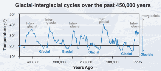
(I’d post it but for some reason I can’t add pictures to my replies)
that graph is very much a sinusoid. A complex one to be sure but still sinusoidal. Think of someone hitting all the black keys on a piano. What you will get is a complex waveform but it is *still* sinusoidal, rising and falling, up and down.
There’s no “statistical significance” associated with periodic sinusoids.
From https://math.ucr.edu/home/baez/glacial/glacial.pdf: “Nonetheless, a Fourier transform of Earth’s climate data shows peaks at frequencies close to those of the Milankovich cycles!”
As usual you are way out of your depth when it comes to physical science. Give it a rest! Stop digging yourself into a hole!
“Why do you persist in getting on here and showing just how ignorant you are of physical science?”
Fine words coming from someone who thinks the derivative of x/n is 1, and claims that standard deviations can be negative.
I fully accept that electrical engineering is not one of my strong points, and maybe you are using a different definition of sinusoidal to mine. But if so, could you supply your definition, as everything I can find just says that sinusoidal means shaped like a sine wave. You seem to think it means anything that can be produced by adding multiple sine waves. E.g.
“Of course it is! A square wave is made up of sinusoids. A triangle wave is made up of sinusoids.”
Yet Wikipedia says
“I always forget just how ignorant you are of basic math. A combination of sinusoids is itself sinusoidal.”
I’ll take that as a no, you didn’t mean “complex”. As to “any combination of sinusoids is itself a sinusoid” – could you provide a reference. I thought that was only the case when all the sinusoids have the same frequency.
But regardless of your definition of sinusoidal, it’s still statistically inept to assume that just because you can combine an infinite number of sine waves to deconstruct a time series, that means you have an accurate model. As I said before, you are demonstrating the dangers of over fitting. Fourier Analysis means you can produce any curve you like given enough waves. You can draw Fourier’s face using a large number of complex sine functions. That doesn’t mean those sines explain his face, or that his face is actually made up of sine waves.
As I asked before, if you want to convince me this is a good model, then do the work. Work out what the sine waves are that would fit temperatures up to a certain date, then see how good they are at predicting the rest of the data.
We were here before a few months ago, with that article claiming half a dozen sine waves was a better fit for the data, than CO2. Problem is, that when you project backwards and forwards a few hundred years, you would be getting anomalies of ±40°C. I’m sure this is the sort of non-physical nonsense that some would dismiss as “trendology”.
There are times when it makes sense to think in terms of sinusoids – such as seasonal variation in the short term, Milankovitch cycles in the longer term. Because the orbit of the earth produces natural cycles. What’s wrong is to just assume from that you can explain all climate change to these cycles, rather than accept that maybe there is a more linear relationship between factors.
“But regardless of your definition of sinusoidal, it’s still statistically inept to assume that just because you can combine an infinite number of sine waves to deconstruct a time series, that means you have an accurate model. “
You are so lost in the trees that you can’t see the forest. The Milankovitch cycle is not a “model”. A Fourier or wavelet analysis of the such is *not* a model.
“You can draw Fourier’s face using a large number of complex sine functions. That doesn’t mean those sines explain his face, or that his face is actually made up of sine waves.”
Did you actually read this before you posted it?
Typical cognitive dissonance from you.
“As I asked before, if you want to convince me this is a good model, then do the work. Work out what the sine waves are that would fit temperatures up to a certain date, then see how good they are at predicting the rest of the data.”
I don’t *need* to work it out. I *know* that a complex sinusoid can be broken down into component sine waves using Fourier or wavelet analysis. *YOU* are the one trying to say that it is impossible to do, not me.
” Problem is, that when you project backwards and forwards a few hundred years, you would be getting anomalies of ±40°C. I’m sure this is the sort of non-physical nonsense that some would dismiss as “trendology”.”
Oh, malarky! The issue is having the total signal to break down rather than just a piece of it. What happens in a hundred years depends as much on low frequency components as it does on the higher frequency components. You can’t identify the low frequency components of climate from a 30 year sample. Fourier or wavelet analysis is *NOT* trendology.
You are *still* demonstrating your lack of understanding of the real world. Keep it up. Your credibility just gets worse with every post you make!
“What’s wrong is to just assume from that you can explain all climate change to these cycles, rather than accept that maybe there is a more linear relationship between factors.
More malarky! Anything that cycles can be broken down into piece parts. What you are trying to claim is that climate is no longer a “cycle” but a linear growth headed for being a fireball.
Take a pure sine wave. If all you have is a small increment of signal around the zero point that data will look as if it is linear. But it isn’t. It’s just part of the signal and doesn’t represent a valid sampling. Go look up Go look up the term “Nyquist-Shannon”.
So lost in the trees says someone who quibbles over the word model, as he doesn’t understand what it means.
“Did you actually read this before you posted it?
”
Lost in the trees, he says.
“I don’t *need* to work it out.”
It’s just an article of faith to you.
” I *know* that a complex sinusoid can be broken down into component sine waves using Fourier or wavelet analysis. *YOU* are the one trying to say that it is impossible to do, not me. ”
I’ve just told you it’s possible to do. But if you don’t do it you will never know if it makes sense. What does your Fourier Analysis of the temperature record tell you about the causes of the change? What does it predict for values outside the range?
“Oh, malarky! The issue is having the total signal to break down rather than just a piece of it.”
What does it tell you if the analysis in a piece of the data tells you nothing about the total data? This is one of the main tools of data analysis, testing how well part of the data predicts the rest. It’s a way of avoiding over fitting.
The whole point of May’s analysis was to argue that the fit proved that solar factors where the real cause of the warming, based on the best fit to the existing data. But if the fit produces meaningless values outside that data range, then it’s clear either the sine wave hypothesis is wrong, or your fit is wrong.
“Fourier or wavelet analysis is *NOT* trendology.”
Then of what use is it?
“What you are trying to claim is that climate is no longer a “cycle” but a linear growth headed for being a fireball.”
What I’m claiming is that there can be multiple causes of a changing climate at many different scales – some cyclical some .linear. What I’m trying to establish is why you can be so certain that say a correlation between CO2 and temperature means nothing, whereas a few fitted sine waves tell you everything you need to know.
Saying CO2 is a cause of temperature change does not imply that there will be a linear increase in temperature until we turn into a “fireball”. It’s saying the temperature to some extent depends on the level of CO2. When CO2 stops increasing so does the temperature.
“Take a pure sine wave. If all you have is a small increment of signal around the zero point that data will look as if it is linear.”
Correct. It will also look like a sine wave if you have a linear increment. That’s why it’s important to look at all possibilities and try to determine the most likely.
Now you have devolved into arguing about what the meaning of “is” is.
bellman: “You can draw Fourier’s face using a large number of complex sine functions. That doesn’t mean those sines explain his face”
The subject of your statement is the DRAWING of the face, not the face itself.
“It’s just an article of faith to you.”
Just like Gauss’ Law is an article of faith with me. It’s why it is considered a LAW and not just a theory.
“What does your Fourier Analysis of the temperature record tell you about the causes of the change? What does it predict for values outside the range?”
I don’t need to know the causes to find the components exist! Once you know the components exist *then* you can try and figure out what are causing the components to exist.
You don’t even understand the scientific method and yet here you are trying to lecture about it! The FIRST step in the scientific method is recognizing something that needs explaining. You don’t create a hypothesis first! That’s typically the third or fourth step yet you want to put it first!
“What does it tell you if the analysis in a piece of the data tells you nothing about the total data?”
Stop repeating back to me what I’ve already told you! It makes you look like a parrot!
“Then of what use is it?”
Fourier analysis is *not* a predictive tool, it is an analysis tool. You keep saying you aren’t trying to predict the future based on analysis of current data but then you turn around and do it every single time! It’s why so many financial marketing ads say “past performance is not a guarantee of future results”. Yet *YOU* think every single time that past performance *is* a guarantee of future results.
“What I’m claiming is that there can be multiple causes of a changing climate at many different scales – some cyclical some .linear. “
You don’t even know what you are saying here. Linear functions that continue forever sooner or later wind up exceeding natural limits. Entropy is a linear function that will end in the heat death of the universe. Yet there is no indication in the temperature record of the earth that indicates that it is anything other than a sinusoidal function that oscillates within predictable limits. Up and down and up and down and up and down – and it will continue so as long as the sun maintains its activity.
“Saying CO2 is a cause of temperature change does not imply that there will be a linear increase in temperature until we turn into a “fireball”. It’s saying the temperature to some extent depends on the level of CO2. When CO2 stops increasing so does the temperature.”
And as Monckton has shown, even when CO2 increases the temperature can stop increasing. That is *NOT* a linear function of CO2 and temperature.
“Correct. It will also look like a sine wave if you have a linear increment.”
Huh? You are babbling. How do “linear increments” look like a sine wave?
I think he means that if you look at a sufficiently short section of a pure sine wave it will appear linear. The real question is: of what use is this?
Yep. It’s meaningless.
If you use the points immediately surround the min and max values the slope will be quite close to zero, i.e. a horizontal line. Meaning? That if you look at the max on the curve that you can forecast things will stay the same forever?
Exactly.
“Fine words coming from someone who thinks the derivative of x/n is 1, and claims that standard deviations can be negative.”
You *still* can’t get over the fact that the partial derivative of the function is a weighting factor when used in uncertainty propagation of quotients which you denied. Even after having your face rubbed in it you can’t accept the simple fact that you don’t know calculus and how relative uncertainty behaves during propagation.
Nor can you accept the fact that sqrt(x^2) has TWO ROOTS, +x and -x. Something taught in elementary school math. (+x)^2 = x^2. (-x)^2 = x^2. Standard deviation is the square root of variance and therefore has a positive and negative root.
Standard deviation runs from (mean – x) to (mean + x). Look at this simple graph:
Or this one:
Or this one: https://external-content.duckduckgo.com/iu/?u=https%3A%2F%2Ftse1.mm.bing.net%2Fth%3Fid%3DOIP.MJ7_nzJ4DFKp4J8Wu2nJwQAAAA%26pid%3DApi&f=1&ipt=781b54f032f3af0708d9c62382201f9053f1e5730e2240bc20cb42324226a740&ipo=images
I see he’s now a leading expert in Fourier analysis, as well as metrology.
/snort/
My guess is that he has never, not once, ever used a spectrum analyzer. Probably has never even seen one!
Me: “I fully accept that electrical engineering is not one of my strong points”
Troll: “He’s claiming to be a leading expert in Fourier analyis.”
So much fun. The person who continually throws out “you don;t understand basic math” as an insult – will double down on his own misunderstandings – despite having plenty of opportunity to educate himself.
Note – he carefully avoids actually saying what he thinks the derivative of x/n with respect to x is. He doesn’t deny he thinks it’s 1. He just tries to distract with all this “it’s a weight” nonsense. Why he thinks the purpose of the derivative should alter the result is something only he knows.
Then he throws a strawman out about standard deviations. Claims I don’t understand that a square root can have two values, but ignores the fact that the standard deviation is the positive square root of the variance.
He even quotes the definition of the standard deviation – but still hasn’t learnt, despite this being discussed at tedious length last year that the √ symbol always means the positive square root.
And he really hasn’t accepted the obvious point, that all his graphs showing negative values, are showing the negative of a positive standard deviation. It’s like he sees a number line showing -3, -2 etc, and saying this proves that 3 and 2 are negative numbers.
” Claims I don’t understand that a square root can have two values, but ignores the fact that the standard deviation is the positive square root of the variance.”
Are we still doing that?
DUDE!! Scientific, engineering evaluations are replete with meaning free, thrown out roots. Looks like one more chapter in that book “What’s the matter with Kansas”.
Somehow those with blinders can’t see the negative numbers in the graph above.
Or this one:
Or this one:
There are none so blind as those who will not see.
Who are “we”, blob?
The ‘Royal We?’
Indeed,
You just can’t admit you got caught not understanding how the partial derivative becomes a weighting factor – even after I showed you the math NOT TWICE BUT THREE DIFFERENT TIMEES!
Here it is again =-=
let y = x/n
What are the relative uncertainties?
The relative uncertainty equation becomes:
[ u(y)/y ]^2 = [(∂y/∂x)^2 * u(x)^2 ]/xx^2 since n, being a constant, has no uncertainty.
If the partial derivative of ∂y/∂x is 1/n we get
[u(y)/y]^2 = ([1/n)^2 * u(x)^2 ] / x^2
So u(y)^2 = [ (1/n)^2 * u(x)^2] / y^2 –>
Since y = x/n, y^2 = x^2/n^2
Now you work out what happens when you divide (1/n^2) by (1/n^2) and tell us all.
(hint: the weighting factor provided by the partial derivative becomes 1 (ONE).
Exactly what Possolo did which you simply could not understand. You are *still* saying I did the math wrong and I don’t know how to get a derivative – when the fact is that you don’t understand how to do relative uncertainty. You have the temerity to imply that Possolo’s calculation was wrong!
“You just can’t admit you got caught not understanding how the partial derivative becomes a weighting factor – even after I showed you the math NOT TWICE BUT THREE DIFFERENT TIMEES!”
So embarrassing for a grown man to be so childish over something he doesn’t understand. Call it a weighting factor if it makes you feel better – it;s really a scaling factor, but it makes no difference to the value of the partial derivatives.
“let y = x/n”
OK. That’s really simple. Even Tim shouldn’t be able to get that one wrong. Just go to equation 10, plug in the uncertainties and the partial derivative and Bob’s your Uncle.
Using the function f(x) = x/n
u(y)^2 = (∂f/∂x)^2 * u(x)^2
and as ∂f/∂x = 1/n, we get
u(y)^2 = [u(x) / n]^2
so
u(y) = u(x) / n
Just as Taylor said all those years ago.
.
So lets see how Tim gets on.
“What are the relative uncertainties?”
OK, what have relative uncertainties got to do with this? But obviously the relative uncertainty of y is
u(y) / y = [u(x) / n] / y
which translates to
u(y) / y = u(x) / x.
Makes sense as y is just a scaling of x, the relative uncertainties are the same for both x and y.
Back to Tim.
[ u(y)/y ]^2 = [(∂y/∂x)^2 * u(x)^2 ]/xx^2 since n, being a constant, has no uncertainty.
I’m not sure what equation he is using here. Equation 10 isn’t about relative uncertainties.
“If the partial derivative of ∂y/∂x is 1/n we get”
It’s not a matter of choice, it’s what it is.
[u(y)/y]^2 = ([1/n)^2 * u(x)^2 ] / x^2
So u(y)^2 = [ (1/n)^2 * u(x)^2] / y^2
what just happened? You’ve divided through by y^2, but somehow lost the x^2
u(y)^2 = {[ (1/n)^2 * u(x)^2] / x^2} / y^2
and substituting x/n for y
u(y)^2 = [ (1/n)^2 * u(x)^2] / (x^4 * n^2)
or
u(y) = [u(x)/x] / n^2
Which is wrong, and either I’ve made a mistake, or Tim’s mystery equation at the top was nonsense.
“Now you work out what happens when you divide (1/n^2) by (1/n^2) and tell us all.”
Surely even you can work out it’s 1.
“(hint: the weighting factor provided by the partial derivative becomes 1 (ONE).”
The mental knots some people will tie themselves in, just to prove an incorrect result. I’ve given you the correct answer above.
u(y) = u(x) / n.
Thew “weighting” factor is 1/n.
It’s not a problem that you don’t understand this. It is a problem that you refuse to learn, and accuse anyone trying to correct you as “not understanding basic math”.
“Exactly what Possolo did which you simply could not understand.”
That is not remotely what Possolo did, or anyone else who knows how to read an equation for that matter. I’ve explained to you several times how to correctly use the equation to get to the standard uncertainty for the volume of a cylinder.
Rest of hysterical childish tantrum ignored.
“OK, what have relative uncertainties got to do with this? But obviously the relative uncertainty of y is”
You have never bothered, not once, to actually study Taylor over the past two years.
Relative uncertainties are used primarily in two different scenario’s:
“u(y) / y = [u(x) / n] / y”
This is *NOT* the relative uncertainty equation that applies!
u(y)/y = ([u(x)/x)/n)] is the equation that applies.
And it is *still* nothing more than the average relative uncertainty which is *not* the uncertainty of the aveage!
Relative uncertainties are percentages. They are the absolute uncertainty divided by the absolute value of the measurement. In this case y is *NOT EQUAL* to y. You can’t just substitute y for x.
I’m not even going to bother addressing the rest of your post. You have no idea what you are talking about and you refuse to learn. You *NEED*, just absolutely *NEED* to study Taylor in detail and work out each and every problem in the book before you can speak intelligently about uncertainty.
YOU BEEN TOLD TO DO THIS MULTIPLE TIMES AND YOU REFUSE TO DO IT.
Instead you just cherry pick things and throw them out with absolutely no understanding of the concepts involved.
Both you and bdgwx need to take remedial algebra. Neither of you can get anything right. He tries to use a percentage (i.e. the relative uncertainty) on the left side of the uncertainty equation but not on the right side. The right side remains a unit measurement and not a percentage.
“You have never bothered, not once, to actually study Taylor over the past two years.”
We were talking about equation 10 of the GUM, or the equivalent one in Taylor based on error propagation. It deals with absolute uncertainty. You cannot, as you demonstrate, just sneak in relative uncertainty and expect it to work. If you could actually figure out how to use the equation as is, you would see how relative uncertainty, when appropriate, results from it.
“Relative uncertainties are used primarily in two different scenario’”
You can never focus on the point in hand. What you are doing is going back to the rules that are derived from the general equation.
““u(y) / y = [u(x) / n] / y”
This is *NOT* the relative uncertainty equation that applies!”
Read my previous comment. I showed you how to use equation 10 for the function you said – y = x / n. this is just u(y) = u(x) / n, then showed you how to convert it to a relative uncertainty. Just telling me it doesn’t apply is just you not understanding algebra.
“u(y)/y = ([u(x)/x)/n)] is the equation that applies.”
Amazing. So you think you can take the equation u(y) = u(x) / n, and divide the LHS by y, and the RHS by x. You are sure you did algebra at school?
“And it is *still* nothing more than the average relative uncertainty which is *not* the uncertainty of the aveage!”
How can it be an average of anything. There is only one x term in the equation, y = x/n.
You really must stop thinking that scaling anything means you are taking an average.
“Relative uncertainties are percentages”
Well, only if you multiply them by 100.
“In this case y is *NOT EQUAL* to y.”
Staggering. (Go on=, keep telling me how I don;t understand basic math.)
“You can’t just substitute y for x.”
I didn’t. I substituted x /n for it.
Rest of childish rant ignored.
“So embarrassing for a grown man to be so childish over something he doesn’t understand. Call it a weighting factor if it makes you feel better – it;s really a scaling factor, but it makes no difference to the value of the partial derivatives.”
You are uneducatable.
Look again at Possolo. In the formula πHR^2, you actually have
πHRR. The uncertainty of H gets added in once and the uncertainty of R gets added in twice. That comes from the partial derivative of R^2 be 2R. When you are doing relative uncertainty you divide by R and so it goes away leaving only 2 * u(R). The uncertainty of R gets added in twice.
That is *NOT* a scaling factor – it is a WEIGHTING FACTOR. You don’t change the value of u(R), you just add it in twice!
“u(y) = u(x) / n”
What happened to the u(x)/sqrt(N)?
u(x)/n IS THE AVERAGE UNCERTAINTY!
It’s what I’ve been trying to tell you and your compatriots like bdgwx from the very beginning.
Somehow you have the idea that the average uncertainty is the uncertainty of the average. IT ISN’T!
“Look again at Possolo.”
Rather than doing that for the 100th time, why don;t you actually look at the equation. I’ve told you this multiple times. You are ignoring what the equation says, and instead trying to refuse engineer it from a single example. You’ve managed to convince yourself you understand how it works, just becasue you get the same result, but in reality that is just an accident. You are treating Equation 10 as if it was about relative uncertainty, doing the sums wrong, and thinking you understand it just becasue you get the right result.
“πHR^2. The uncertainty of H gets added in once and the uncertainty of R gets added in twice.”
That’s the end result, but you don’t understand why.
“that comes from the partial derivative of R^2 be 2R”
But that’s not the correct partial derivative. The function is πHR^2, the derivative with respect to R is 2πHR. That’s your so called weighting factor.
“When you are doing relative uncertainty you divide by R”
But you can’t divide by R without dividing everything else by R. You would have learnt that if you were ever taught algebra.
You get the relative uncertainties by dividing both sides by V^2. That cancels out all the extra terms on both sides and you are left with an equation that is entirely relative.
“That is *NOT* a scaling factor – it is a WEIGHTING FACTOR.”
I’m guessing weighting factor is another of those terms you have your own private definition of. In my definition a weighting factor would mean you have to divide the whole equation by the sum of the weights.
“You don’t change the value of u(R), you just add it in twice!”
You multiply it by 2 if that’s what you mean. I’m guessing you dropped out after they taught you how to multiply by repeated addition. Is this why you have so much difficulty with the concept of dividing the uncertainty by n?
““u(y) = u(x) / n”
What happened to the u(x)/sqrt(N)?”
Why would there be a division by sqrt(N)?
You gave me an example of y = x / n, and that is the result. If you had actually read Taylor, as you keep claiming to have done, you might remember the special case, where multiplying by an exact figure results in multiplying the uncertainty by the same value. This example illustrates that for the exact value 1/n.
“u(x)/n IS THE AVERAGE UNCERTAINTY!“
The bolder the text the wronger the sentence.
No it is not an average uncertainty. It would be if there were n different uncertainties and we added them and divided by n – as P:at Frank does in his pamphlets.
But here we are just taking a single value of n, and dividing it by n. n could be any value you like, you didn’t specify. All it shows is that scaling value will also scale the uncertainty by the same amount – you know, just as I told you all those years ago, when you were trying to claim that scaling the value had no effect on the uncertainty.
“Somehow you have the idea that the average uncertainty is the uncertainty of the average. IT ISN’T!”
Glad you agree that Pat Frank was wrong.
If you want to use equation 10 with an actual average – I’ve told you this a few dozen times before, but I understand how bad your memory is – you would do this.
Add the squares of all the uncertainties and divide each by n^2. Simplifies to divide the sum of the squares of the uncertainties by n^2. Then take the (positive)square root leaving you with
√[u(x1)^2 + u(x2)^2 + … + u(xn)^2] / n
And for the special case where all the uncertainties are the same size, u(x), we get
√[n * u(x)^2] / n = u(x) / √n
and that’s where √n, appears.
The understatement of the week — his religious dogma tells him what he already believes, anything else must be rejected.
I see someones desperate for attention again.
ALGEBRA MISTAKE #31
[ u(y)/y ]^2 = [(∂y/∂x)^2 * u(x)^2 ]/xx^2 does not follow from Taylor equation 3.47, JCGM 100:2008 equation 10, or anything other equation using a partial derivative.
ALGEBRA MISTAKE #32
u(y)^2 = [(1/n)^2 * u(x)^2] / y^2 does no follow from [u(y)/y]^2 = ([1/n)^2 * u(x)^2 ] / x^2 and y = x/n regardless of how you got to this point to begin with.
Fix the mistakes and resubmit for review.
ALGEBRA MISTAKE #31
ALGEBRA MISTAKE #32
Film at 11—beegee makes another lits.
Clown.
He doesn’t even realize he is using a percentage on one side, u(y)/y but not a percentage on the other side.
And then he uses y on the right side as if y = x when that is not the equation he started with. y cannot equal both x and x/n!
You are kidding, right?
Why did you divide by y on the left side making it a relative uncertainty but didn’t use a relative uncertainty on the right side?
What is “xx^2″?
“[ u(y)/y ]^2 = [(∂y/∂x)^2 * u(x)^2 ]/xx^2 does not follow from Taylor equation 3.47,”
If you use relative uncertainty on the left side, i.e. u(y)/y then you must use relative uncertainty on the right side.
The relative uncertainty on the right side is u(x)/x. When squared this becomes u(x)^2/x^2
Taylor’s Eq 3.47 is *NOT* using relative uncertainty. There is no ẟq/q in 3.47! Or as you put it [u(y)/y]^2
Taylor’s Eq 3.47 is actually:
ẟq^2 = [∂q/∂x]^2 * ẟx^2
Exactly what the GUM equation says.
You are the one that has a problem with algebra, not me. You can’t even keep relative uncertainty used with a quotient/product differentiated from the straight uncertainty of a sum.
Do you even know what a percentage is?
I didn’t. It’s your math. You tell us.
It’s your math. You tell us.
Yes. You made 2 algebra mistakes. One is so trivial even middle schoolers could spot it. I’m asking you to fix the mistakes and resubmit for review.
Another a$$hat.
bdgwx doesn’t even understand how Monte Carlo simulations *work*. The random numbers are samples drawn from a large database. As such, the CLT says they will tend to a Gaussian distribution. A Gaussian distribution is *NOT* what you see for systematic bias in real world temperature measuring devices, it will be asymmetric and the only question is how asymmetric it is. Since bdgwx and climate science never worry about the actual data distribution and just assume it is Gaussian they will never know how asymmetric either their data or the associated measurement uncertainty is. I have pointed this out to bdgwx TWICE in the past and he is either apparently unable to learn or wishes to remain willfully ignorant.
Taylor gets into this in his Chapter 7 on weighting averages and Bevington in Chapter 5 on Monte Carlo simulations. It’s pretty apparent that no one on here supporting current climate science has ever studied any of the three leading authors on metrology that I have found, Taylor, Bevington, and Possolo.
“a$$hat” is right.
Among many other things, they cannot get past the fact that glomming air temperature data together is not an exercise in Stats 101 random sampling. They hand-wave that it is random sampling over and over and over and over.
At this point I can only conclude that climate so-called science is actually a religion.
Keep on lying.
I’ve repeatably pointed out that the temperature data sets are not based on random sampling, and that nobody calculates their uncertainty by dividing the standard deviation by root-n.
Bullcrap. You were right in there with bdgwx trying to say that the standard deviation of the sample means is the measurement uncertainty of the average.
Shows how little you can remember of what I tell you.
No, what it shows is how little you want to admit to saying.
Yep, a distinction without a difference.
oily bob is waving his arms back-and-forth about how adding more and more thermometers together magically makes systematic uncertainties transmogrify into random ones, which then disappear.
All of this is from stats sampling and the SEM, and they all maintain the same fiction.
No algebra mistakes by me, only you.
You continue to divide by sqrt(n) when it should be n. In other words you keep calculating the average uncertainty and claiming that is the uncertainty of the average. It isn’t.
“Standard deviation runs from (mean – x) to (mean + x). Look at this simple graph:”
Cripes, you are thick. That graph does not show negative standard deviations. It shows the distribution variable in units of (positive) standard deviation.
Nitpick Nick tries to rescue his acolyte!
OK, do you think it shows negative standard deviations?
Oh look, negative numbers:
https://wattsupwiththat.com/2024/04/02/uah-global-temperature-update-for-march-2024-0-95-deg-c/#comment-3892348
What you lot missed in your haste to cherrypick the GUM, is that while standard combined uncertainty is calculated with the positive root, the negative root returns when calculating the expanded uncertainty, which is always expressed as ±u_c * k = ±U.
“Oh look, negative numbers:”
Where? I see standard deviation σ multiplied by positive or negative integers. But σ is positive.
“ ±U”
Yes, but U is positive.
And why are you quoting the GUM. You and your merry band of clowns don’t believe uncertainty even exists, much less propagates.
A negative integer isn’t a negative number?
ROFL!!
Nick apparently doesn’t think -1 is a negative number!
Stokes has declared something, therefore it must be true, and all his ducklings run right behind him.
Or maybe, just maybe, more than one person understands what a standard deviation is, and knows it cannot be negative.
Maybe, just to be on the safe side, some of double check with the source of all knowledge, and see that the GUM agrees that standard deviations cannot be negative.
Maybe, however unlikely it might seem, Pat Frank is wrong about something. Maybe even you are wrong about something.
Stokes duckling is trying to goad me into playing his games.
You didn’t even look at the graph!
Here it is again: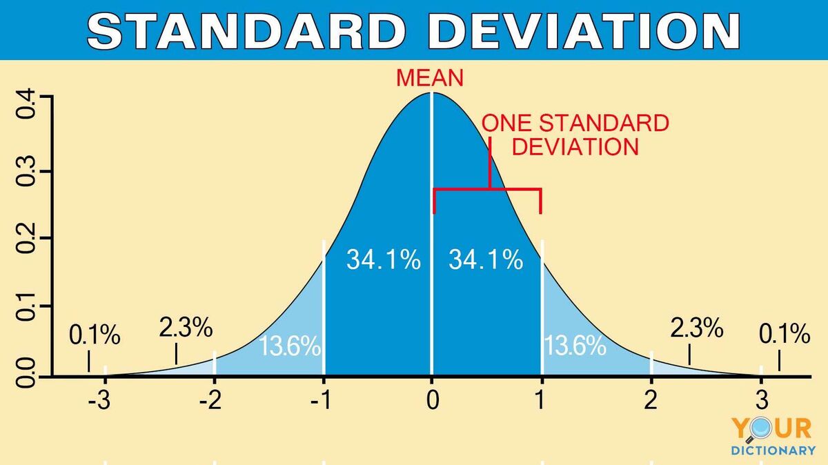
There is both a positive part of the standard deviation and a negative part of the standard deviation. From =1 to +1.
Now tell me that -1 is *not* a negative number!
You have no idea what standard deviation even means. That is just a plot of the probability density function of a standard Gaussian distribution. The standard deviation of the distribution is 1. A single positive number. It says in red. What the graph is pointing out for the Stats 101 class is that 34.1% if the area lies between 0 (the mean) and +1 (the sd). Another 34.1% lies between -1 and 0, leading to the common understanding that 68.2% of instances will lie within 1 sd of the mean (for a Gaussian).
“ Standard deviation is the square root of variance and therefore has a positive and negative root.”
You tell us that only you have a proper understanding of standard deviation, and then come up with this rubbish. OK, here isJCGM:100 2008 (GUM):
Word to the wise. I went down this rabbit whole last summer starting with Pat Frank. Wasted an entire week vending of hundreds of aggressive comments.
No amount of actual evidence will persuade them. Even quoting the precious GUM.
Here’s where the argument started if you want an idea of the mental blocks you are up against.
https://wattsupwiththat.com/2023/08/24/patrick-frank-nobody-understands-climate-tom-nelson-pod-139/#comment-3774135
I hear you.
We’re the mugs.
But it’s fun.
No, you lot are the clowns in Spencer’s three ring circus.
Yes, I’ve been down it with Pat Frank here and elsewhere.
And you’re too much of a leftist-marxist stooge to face reality.
You no more understand the GUM than you understand Taylor, Bevington, or Possolo. You don’t know the difference between absolute uncertainty and relative uncertainty. You think the measurement uncertainty of an average is the standard deviation of the sample means.
There is almost nothing you actually understand about metrology and how it is used.
Neither does Nick or any other advocate of climate models that I have seen here on WUWT. You, and them, can’t even handle simple calculus.
Pat Frank’s career has been in analytical chemistry. He *had* to learn uncertainty in order to properly do his job.
You? You are a cherry picking bystander who thinks measurements are given as “true value +/- error” and that all error is random, Gaussian, and cancels.
You can’t even tell when you are calculating an average uncertainty and when you are calculating the measurement uncertainty of the average.
You don’t even know that calibration labs don’t give you a 100% accurate calibration, that their results are given with an uncertainty interval. In other words no real world measuring device starts off with “true value” indications – not even at the door to the calibration lab.
You have absolutely no credibility and no standing to criticize anyone else’s knowledge of metrology.
“You no more understand the GUM than you understand Taylor, Bevington, or Possolo.”
Coming from you that’s a complement.
Just answer one question. Does the GUM say that standard deviations are always positive?
“Pat Frank’s career has been in analytical chemistry. He *had* to learn uncertainty in order to properly do his job.”
Argument by authority – yet you never extend that logic to other professions.
“You are a cherry picking bystander who thinks measurements are given as “true value +/- error” and that all error is random, Gaussian, and cancels.”
You just lie and lie.
“You can’t even tell when you are calculating an average uncertainty and when you are calculating the measurement uncertainty of the average.”
One day you are going to actually read what Frank says, and realize what an idiot you are. (You won’t).
His whole argument is that the uncertainty of the average is the average uncertainty.
“You have absolutely no credibility and no standing to criticize anyone else’s knowledge of metrology.”
Apart from understanding the maths, and when it’s being abused.
“Pat Frank’s career has been in analytical chemistry.”
Look it up. The pinnacle of his “career” was the proper administration of lab waste. SLAC told it’s staff that if they had questions about that, then he was the go to guy. A vital job to be sure…
blob chimes in with a slime on the enemy of the state religion.
Unable discredit his work, now these pricks have to stoop to posting personal info as if it proves “something”.
And he wonders why he has had nada besides autoerotic cites for his last 2 papers. But he is wearing a nifty chapeaux in the post pic in your link..
You’re a total prick, blob. You and bellcurvewhinerman are two peas in the same pod.
Congratulations! You may already be a whiner!! But if you keep this up you might besmirch WUWT’s hard earned rep for posting only serious, data based, comments.
Jeez, you can’t even make a sartorial compliment these days…
And diss me, and only me, when responding to me. I have nowhere near the acumen and knowledge of the other posters here who have exchanged views with Dr. Frank. My only use is as coal mine canary. By the time even I can see thru his muck, he’s in Homer S. territory.
I’m not the one posting personal information trying to slime someone’s reputation, a##hat.
Go lick Stokes’ boots some more.
Wut “personal information”? The SLAC site was public. I found it in 30 seconds, with no sign in. And please, what’s wrong with being the guru of lab waste disposal?
At this point you should be feeling really lucky the moderators don’t boot your fat arse for doxing, blob.
They should.
What does the GUM say about expanded uncertainty, Nitpick?
Only a flesh wound…
“I fully accept that electrical engineering is not one of my strong points”
It’s not just electrical engineering! It’s the real world. The resulting tone from hitting two different keys on a piano has nothing to do with electrical engineering. The pressure pulses in an automobile exhaust pipe are sinusoidal but have nothing to do with electrical engineering. In my younger days I raced motorcycles with 2-cycle engines. It was imperative to understand the sinusoidal pressure waves, their interference patterns, etc. in order to get the vacuum part of the pulse at the exhaust port of the cylinder right when the exhaust valve was opening in order to get the best scavenging of the combustion products resulting in the best horsepower output at the desired rpm.
The fact is that you have *no* knowledge of the real world and how it works. I almost used the words “almost no knowledge” but your total ignorance of the real world prevents using the word “almost”.
” maybe you are using a different definition of sinusoidal to mine.”
Stop the incessant whining and excuse-making. Sinusoidal has exactly one definition, up and down. If your definition is different than that it is wrong, not just different.
“But if so, could you supply your definition, as everything I can find just says that sinusoidal means shaped like a sine wave. You seem to think it means anything that can be produced by adding multiple sine waves. E.g.”
You seem to be confusing the terms “sine” and “sinusoidal”. That is typical for you.
go here:
Does that look like a sine wave to you? Yet it is a representation of the VIBRATION in a machinery gear. The term “vibration” implies sinusoidal, i.e. oscillation around an equilibrium point, even if it doesn’t look like a pure sine wave!
“Yet Wikipedia says”
Don’t believe everything wikipedia has to say. That definition *should* say that a square wave is not a sine wave, but it *is* sinusoidal. I would also point out that there is no such thing as a pure, ideal square wave in the real world most of us live in. Wikepedia goes on to talk about square waves being used in the digital world. And yet every single digital circuit I have ever worked on will respond to a sine wave of the appropriate amplitude just like it will to a square wave. That’s because the digital circuits respond to a signal amplitude, not a signal shape.
“I’ll take that as a no, you didn’t mean “complex”. As to “any combination of sinusoids is itself a sinusoid” – could you provide a reference. I thought that was only the case when all the sinusoids have the same frequency.”
ROFL!! If you throw two different size rocks into a pond at different locations they will each generate a wave of different frequencies. Yet when they interact they will form a sinusoidal interference pattern. Stroke two different strings on a violin and you will get different frequencies from each – yet their combination produces a sinusoidal interference wave – a “complex” sinusoid.
I’ll repeat, I simply don’t understand why you insist on coming on here and demonstrating your total lack of understanding of the real world. Yet you insist on lecturing people on how they are wrong even when you have no basic knowledge of the subject you are discussing.
Most people would be embarrassed to do this but not you.
To include lecturing Pat Frank about uncertainty, when he can’t grasp basics such the inability to know true values of measurements.
Yep.
“It’s not just electrical engineering! It’s the real world.”
Yes there are lots of real world uses. But that doesn’t mean you can apply it top everything. You are sounding like the classic, “all you have is a hammer so everything looks like a nail” cliche.
“Stop the incessant whining and excuse-making. Sinusoidal has exactly one definition, up and down.”
A link to that “one” definition would help your argument. So would avoiding all these petty insults.
“Does that look like a sine wave to you?”
Does your quote say it’s sinusoidal? It’s a complex analytical signal. No mention of it being sinusoidal.
“Don’t believe everything wikipedia has to say.”
I don’t. But I trust it more than would your pronouncements.
“That definition *should* say that a square wave is not a sine wave, but it *is* sinusoidal.”
Then all you have to do is provide a link to a reference saying that. Maybe you are correct, but I’m not going to take that on trust.
I have tried to find different definitions, I’m sure there’s a good chanced I’m wrong, and this is a distraction from the real point in any case. But so far, I just keep finding things like
https://www.allaboutcircuits.com/textbook/alternating-current/chpt-7/square-wave-signals/
https://www.electronics-notes.com/articles/basic_concepts/electronic-electrical-waveforms/square-waveform-rectangular-pulsed.php
“ROFL!! If you throw two different size rocks into a pond at different locations they will each generate a wave of different frequencies. Yet when they interact they will form a sinusoidal interference pattern. Stroke two different strings on a violin and you will get different frequencies from each – yet their combination produces a sinusoidal interference wave – a “complex” sinusoid. ”
I see you still don’t understand what “complex” means – despite quoting a passage about complex signals.
“Yet you insist on lecturing people on how they are wrong even when you have no basic knowledge of the subject you are discussing.”
Says someone who’s constantly lecturing climate scientists and statisticians on why they are wrong.
A complex sinusoid is of the form:
Acos(wt+ⱷ) + jAsin(wt+ⱷ)
However, in the general form the coefficients can be A *and* B and w doesn’t have to be the same for each.
Assuming the stated value of a measurement is 100% accurate so you can ignore the measurement uncertainty of the measurement *IS* wrong, and yet climate science and statisticians do it all the time.
“Yes there are lots of real world uses. But that doesn’t mean you can apply it top everything.”
Of course you can. Everything that goes up and down and up and down and up and down can be decomposed into sine waves. It’s the whole concept of Fourier and wavelet analysis. All you are saying here is that Fourier and wavelet analysis don’t work – no matter how many people use them every single day.
“A link to that “one” definition would help your argument.”
You like wikepedia? Here is what it says about Fourier analysis:
“In mathematics, Fourier analysis (/ˈfʊrieɪ, -iər/)[1] is the study of the way general functions may be represented or approximated by sums of simpler trigonometric functions.”
“Fourier transforms are not limited to functions of time, and temporal frequencies. They can equally be applied to analyze spatial frequencies, and indeed for nearly any function domain. This justifies their use in such diverse branches as image processing, heat conduction, and automatic control.”
“Does your quote say it’s sinusoidal? It’s a complex analytical signal. No mention of it being sinusoidal.”
Either you can’t read or you don’t bother to read. The graph was for mechanical VIBRATION! Vibrations *are* a sinusoidal function. You can’t even read the graph properly! Yet here you are trying to tell people that they are wrong about sinusoidal functions.
“Then all you have to do is provide a link to a reference saying that.”
The Fourier analysis of a sine wave is:
f(x) = (4/pi) Σ (1/n) sin(nπx/L) where n is all the odd numbers from 1 to infinity. L is 1.2 the period of the square wave.
Since a square wave is a function composed of sine waves it is a sinusoidal function! Voila! QED. No reference needed!
“It has been found that any repeating, non-sinusoidal waveform can be equated to a combination of DC voltage, sine waves, and/or cosine waves (sine waves with a 90 degree phase shift) at various amplitudes and frequencies.”
Now you have been reduced to cherry-picking again. It’s obvious that you don’t have a clue as to what this is actually saying.
It should be obvious that the phrase “It has been found that any repeating, non-sinusoidal waveform” is nonsensical. The definition says non-sinusoidal while saying it is composed of sine waves! All the DC component does is offset the baseline, it has no bearing on the REPEATING part of the function! My guess is that you don’t even know what sin(x) + cos(x) *is*! (hint: it is a sin function!)
You didn’t even bother to read the sentence after the one you quoted: “In particular, it has been found that square waves are mathematically equivalent to the sum of a sine wave at that same frequency, plus an infinite series of odd-multiple frequency sine waves at diminishing amplitude:”
A signal that is composed of sine waves *is* sinusoidal. There simply isn’t any way around that.
STOP CHERRY PICKING STUFF YOU HAVE NO KNOWLEDGE OF. YOU JUST WIND UP LOOKING STUPID.
“Everything that goes up and down and up and down and up and down can be decomposed into sine waves.”
You can do that – it doesn’t mean you are discovering anything useful.
“All you are saying here is that Fourier and wavelet analysis don’t work – no matter how many people use them every single day. ”
Pathetic use of a straw man. What I’m saying is just becasue you can decompose a time series into an arbitrary collection of sine waves, does not mean you have proven that the time series is driven by sine waves. It’s the same with fitting a high order polynomial. You can get a good fit, you can use that equation for somethings, but you shouldn’t assume you have explained why the time series is behaving as it does. The same with any curve fitting exercise.
“You like wikepedia? Here is what it says about Fourier analysis:”
Yet somehow you forgot to quote the part where it says “Sinusoidal has exactly one definition, up and down.”. Maybe because it never says that. Indeed it never mentions sinusoidal, and only refers to sinusoids as components that make up the function.
It would really help you if you just occasionally excepted you’ve misunderstood something.
“Either you can’t read or you don’t bother to read. The graph was for mechanical VIBRATION! Vibrations *are* a sinusoidal function.”
Talk about a circular argument.
“Since a square wave is a function composed of sine waves it is a sinusoidal function! Voila! QED. No reference needed!”
And again.
“Now you have been reduced to cherry-picking again. It’s obvious that you don’t have a clue as to what this is actually saying. ”
Let me help you. You say that any combinations of sinusoides is sinusoidal. I quote something that says non-sinusoidal functions can be decomposed into sinusoids. Anyone who can see beyond their own ego might realize that this implies that not all combination of sinusoids is sinusoidal.
“It should be obvious that the phrase “It has been found that any repeating, non-sinusoidal waveform” is nonsensical. The definition says non-sinusoidal while saying it is composed of sine waves! ”
And your circular logic continues. Your definition is right, therefore anything that disagrees with your definition must be wrong. QED.
“You can do that – it doesn’t mean you are discovering anything useful.”
Really? A man named Fourier discovered this. And you think it is not useful? WOW!
“What I’m saying is just becasue you can decompose a time series into an arbitrary collection of sine waves, does not mean you have proven that the time series is driven by sine waves.”
You are deflecting. The issue is that a repeating waveform *is* a sinusoid, no matter what the definitions you found say. I gave you the formula for a square wave – the only function in that formula is “sin”. It is the *sin” function components that are driving the square wave. I suspect what you really mean is that you don’t know what is driving the component sine waves. You just don’t want to admit that openly because it would mean that climate science doesn’t have a clue as well. As I’ve already pointed out, you don’t need to know what is driving the sine waves in order to identify that they exist. That *is* the scientific method, observe first, then question what you observed, and then create a hypothesis for the cause.
Please tell us how a continuing oscillating waveform can be created without the use of continued oscillating sine waves. For that is what you are really trying to claim.
“You can get a good fit, you can use that equation for somethings, but you shouldn’t assume you have explained why the time series is behaving as it does. The same with any curve fitting exercise.”
The Fourier analysis is *NOT* a curve fitting exercise. It can be used to identify things that need to be filtered out in order to make the waveform more useful, e.g. remove interfering signals. Nor is this just for electronics. It can be used to analyze vibrations in mechanical objects such as airplane wings, or even automobiles, in order to eliminate unwanted ones. You first have to “observe” the vibrations, then you analyze them, *then* you identify the cause. The scientific method at work.
I’m truly interested. Why do you continue to come on here and demonstrate your total lack of knowledge of the real world, physical science in particular.
Like this: “Maybe because it never says that. Indeed it never mentions sinusoidal, and only refers to sinusoids as components that make up the function.”
This can only mean that you think sinusoids can combine to create something that is not itself a sinusoid. Please tell everyone just exactly how that happens. Demonstrate the math!
“Talk about a circular argument.”
So you think vibrations are not sinusoidal? Tell us what vibrations exist in the real world that are not sinusoidal. My guess is that you will ignore this request.
“And again.”
Apparently meaning yo don’t think the formula for a square wave is made up of sine waves. Even after having been given the functional relationship. There are none so blind as those who refuse to see.
“You say that any combinations of sinusoides is sinusoidal. I quote something that says non-sinusoidal functions can be decomposed into sinusoids. Anyone who can see beyond their own ego might realize that this implies that not all combination of sinusoids is sinusoidal.”
Then give us just ONE EXAMPLE of a combination of sine waves that is not itself a sinusoid. Even the impulse function is a combination of sine waves with an infinite period, i.e. a sinusoid.
Stand by your assertion – give us just ONE EXAMPLE, that’s all, just ONE.
“Your definition is right, therefore anything that disagrees with your definition must be wrong. QED.”
I’ve SHOWN you how the definition is wrong, such as a square wave not being a sinusoid. The formula for a square wave stands mutely as proof – but you just can’t accept that. Again, there are none so blind as those who refuse to see.
“Really? A man named Fourier discovered this. And you think it is not useful? WOW!“
If it helps you understand the words, assume there was an implied “necessarily” in my comment.
You can decompose anything that goes up and down – it doesn’t necessarily found anything useful. And by useful. I mean something that explains why the thing was going up and down. Of course it’s useful for compression.
“You are deflecting.”
Says someone who immediately deflects to his spurious definition of sinusoidal.
“It is the *sin” function components that are driving the square wave.”
Is the Tim who thinks this the same Tim who is constantly pointing out that just because you can show a correlation doesn’t mean you have proven causation.
“I suspect what you really mean is that you don’t know what is driving the component sine waves.”
That and I’m saying you’ve no evidence that those sine waves exist, outside of a mathematical abstraction.
“Please tell us how a continuing oscillating waveform can be created without the use of continued oscillating sine waves.”
No expert, but of the top of my head – put a light source on a bench and measure the light intensity. Then Put a wheel with slits between the light source and the receptor and spin it. I’m guessing the receptor will show something close to a square wave, but at best you can only say there is a single sine wave ion the form of a spinning wheel.
“The Fourier analysis is *NOT* a curve fitting exercise.”
Really? Everything you describe is based on curve fitting. The only difference between what you are describing and say a linear regression, is that in your examples you are assuming a continuous repeating patter, whereas in other time series repetition may only be part of the fit.
“I’m truly interested. Why do you continue to come on here and demonstrate your total lack of knowledge of the real world, physical science in particular.”
I like irony.
“This can only mean that you think sinusoids can combine to create something that is not itself a sinusoid.”
Depends on your definition. Going by your personal definition then obviously no. By your definition every combination of sinusoids is a sinusoid.
Going by everybody else’s definition, yes. The combination of multiple sinusoids is not necessarily or even usually a sinusoid.
Going by the other definition of “Any of the venous cavities through which blood passes in various glands and organs, such as the adrenal gland and the liver.”, then I’m not sure.
Amazing how you can get different answers just by changing the definition.
“Then give us just ONE EXAMPLE of a combination of sine waves that is not itself a sinusoid.”
You’re just going round in circles. You have already admitted that a square wave can be described a combination of sine wave. A square wave is not a sinusoid. There’s ONE EXAMPLE.
If you want to use your own personal definition of sinusoid then you can say I, and the rest of the world are wrong. It’s just odd to get so upset just because no-one is using your own personal definition.
“I’ve SHOWN you how the definition is wrong, such as a square wave not being a sinusoid.”
Asserting is not showing. It’s just a circular argument. You define square waves as sinusoids, then use that to prove that any definition that says it is not a sinusoid must be wrong.
“Again, there are none so blind as those who refuse to see.”
And some say you don’t get irony.
“Really? Everything you describe is based on curve fitting.”
Oh my freaking Lord!
Is calculating the acceleration of an object in free fall in a gravity well “curve fitting”?
Desperation time.
“ Sinusoidal has exactly one definition, up and down. If your definition is different than that it is wrong, not just different.”
Sinusoidal
“of, relating to, shaped like, or varying according to a sine curve or sine wave” Merriam-Webster dictionary
“having the form of a sine curve.” Oxford dictionary
“(of a wave) having a regular smooth repeating pattern“
Cambridge dictionary
“having a magnitude that varies as the sine of an independent variable” Collins English dictionary
And many more…..
There are so many poor definitions running around on the internet it is unbelievable.
These definitions would lead one to believe that only a PURE sine wave of constant period and constant max/min values is sinusoidal.
Pluck two different strings on a violin and you *will* generate a beat tone – a TONE you can actually hear. But it will *not* be a “pure” sine wave but it will be a sinusoidal signal. It’s frequency will be constant but its amplitude will vary over time. That amplitude will *not* vary as a sine wave but as the combination of two component sine waves. Even if they are the same frequency but out of phase you will still get a sine wave, i.e. what is the sum sin(x) + cos(x)?
“There are so many poor definitions running around on the internet it is unbelievable.”
then give a link to the correct definition. Or is this another case where you just know you a right, and so the rest of the world must be wrong.
I gave you the formula for the Fourier analysis of a square wave. What else do you need?
Each and every one of the definitions you found equate the terms “sinusoid” and “sine* wave. They are NOT the same thing. They all state that “non-sinusoidal” signals are made up of sine waves.
Cognitive dissonance at its finest!
Nothing. It’s abundantly clear from your inability to provide a single reference stating that sinusoidal means anything that goes up and down, that you are wrong. You might even know you are wrong. But you will never admit it so will drag it on and on, insisting that everyone else is wrong. t
I’ve asked you to give me one example, JUST ONE, of a function that can be broken down into sinusoidal components that isn’t itself sinusoidal, i.e. goes up and own.
I am still waiting!
*YOU* can’t even admit that a square wave, a function that goes up and down, is made of of sine wave (i.e. sinusoidal) components and is, therefore a sinusoidal waveform itself.
go here:
This waveform is certainly *not* a pure sine wave as you want to restrict the term “sinusoid” as being. It’s minimum and maximum values change with time. It is even labelled “sinusoidal amplitude modulation”.
I quote from the document: “In the case of sinusoidal AM we have”
“I’ve asked you to give me one example, JUST ONE, of a function that can be broken down into sinusoidal components that isn’t itself sinusoidal, i.e. goes up and own.
I am still waiting!”
Grow up. I gave you the example of a square wave.
Of course that won’t satisfy you because you’ve admitted you are making up your own definitions. You are Humpty Dumpty, words mean whatever you want them to mean. So if you want to claim that a victory be my guest. You are correct that if you define all curves that go up and down as sinusoidal, then yes all curves that go up and down are sinusoidal by that definition.
Why you think these hissy fits actually mean anything I can’t say. Call it what you want, it still doesn’t change the argument. Saying you can decompose any curve into sinusoids doesn’t mean those sinusoids have to have any real world meaning.
“sinusoidal amplitude modulation”
You’re as clueless about language as you are about everything else. The name does not mean the wave is sinusoidal it is a type of modulation produced by combining sinusoids. You avoided actually linking to the document. But I guess it’s this
https://www.dsprelated.com/freebooks/mdft/Sinusoidal_Amplitude_Modulation_AM.html
Click on the red “sinusoidal” in the title, and it takes you to the definition:
Good luck claiming that describes a square wave.
“There are so many poor definitions running around on the internet it is unbelievable.”
And yours is one of them, the definitions I quoted were from internationally recognised dictionaries not ‘the internet’.
And not one of them can explain why a square wave goes up and down!
They’re definitions of an adjective, they don’t have to explain anything, if it’s a square wave that’s what you call it.
Fourier demonstrated that any varying time-series can be represented by the sum of a series of sinusoids. He even showed how to do it. There is no danger of “over fitting” a Fourier decomposition. It is what it is.
“Fourier demonstrated that any varying time-series can be represented by the sum of a series of sinusoids.”
Exactly – represented. But that doesn’t mean the sinusoids are real, as in having a real cause. There are cases where it is true that the time series really is made up of many repeating sine waves – sound for instance.
The fact that any time series can be represented in this way should make it clear that it cannot be assumed that the sinusoids caused the time series.
I can create 100 points that are just a straight line, and an FFT can decompose it into 100 sine waves that perfectly represent each of those points – but we know they didn’t cause the straight line, they are just a way of representing it.
Its easier to just ignore data that doesn’t fit than to actually try to think about what they are looking at.
They don’t have the mathematical foundation to understand what they looking at. They just pretend they do. My guess is that they don’t even understand the difference between Fourier analysis and wavelet analysis of a complex waveform.
I’m on his “contrarian” list, so bgwxyz feels justified in ignoring anything I or you write. But make no mistake, he is reading.
First…it’s not per decade. It’s per decade squared. Second…it’s absurd either way. The units are what they are because of the math. And for the record, +0.05 C.decade-2 is exactly the same as +5 C.century-2 or +0.0005 C.year-2. I’m no more predicting 10 years in the future as I am 1 year or 100 years or anything other value. It is the acceleration value now; not the past nor the future.
No backpedaling from me. I stand by what I said. I’ll repeat it again I did a 2nd order polynomial regression on the data. The warming is now accelerating by +0.05 C/decade^2. That is a fact.
So the acceleration tomorrow may be different than the acceleration today?
Why didn’t you say that to begin with? It kind of makes your calculation of the current acceleration useless unless it means something for the future.
As usual, you are wanting your cake and to eat it to. You hope people will assume that you calculate the current acceleration so you’ll know the acceleration tomorrow. But you then turn around and say you aren’t trying to forecast the acceleration tomorrow.
implicit /ĭm-plĭs′ĭt/
adjectiveImplied or understood though not directly expressed
Why do so many supporting climate science so bad at math?
T/decade^2 *IS* (T/decade)/decade. That means you *are* using units of T/decade.
“If you are using units of ‘per decade,’ then you are implicitly predicting at least 10 years into the future”
So, when Spencer says the trend is 0.15°C / decade he’s implicitly making a prediction up to 2034? And when Monckton gave his pauses or cooling trends in degrees per century he was implicitly predicting the trend for the next 100 years?
NO! For the umpteenth time Monckton is predicting nothing. He is showing that CO2 growth is *NOT* directly tied to temperature growth. That is not predicting the future. It is criticizing the theory that CO2 is the temperature control knob for the planet!
Climate science is like a vinyl record with a band scratch, playing the same thing over and over till someone bumps the player. What is it going to take to bump climate science out of its scratch-groove that CO2 is the control knob when it’s obvious that it isn’t?
Learn to read the context before being triggered. I was addressing Clyde Spencer’s claim that “If you are using units of ‘per decade,’ then you are implicitly predicting at least 10 years into the future”
Monckton quotes warming rates in degrees per decade, if Spencer was right that means he’s implicitly predicting at least 10 years into the future. I do not think that. Units of per decade are just a measure of the rate of change, not an implied prediction. I’m glad you agree with me on this.
“He is showing that CO2 growth is *NOT* directly tied to temperature growth.”
No he isn’t. Not even he is that dumb. If you think he is, give the exact quote where he says that.
“What is it going to take to bump climate science out of its scratch-groove that CO2 is the control knob when it’s obvious that it isn’t?”
Some evidence that it has no effect on temperature would be a start.
You are so full of it that it’s coming out your ears.
You’ve been lectured on this BY MONCKTON several times before. You are doing nothing but trolling here.
Climate science uses a mis-application of feedback theory to claim CO2 is the temperature control knob. Monckton started out trying to refute this claim. Doing so caused him to start looking at the pauses in temperature that were seen in the late 20th century and in the 21st century.
You’ve never understood feedback theory though Monckton has explained it in detail to you. It’s the same for metrology. All you ever do is get on here and try to entice people into clicking on reply.
What Monckton speaks to is warming from natural causes, not man-made causes and misuse of feedback theory. You don’t understand enough of the basics to even get this right!
“Some evidence that it has no effect on temperature would be a start.”
What is Pete’s name do you think the pauses are?
Nor is he able to comprehend that uncertainty is not error.
It seems to me that there are only two reasons for using units of “per decade.” One is to make the number bigger and scarier, the other is to imply that it will be useful over that amount of time. When one calculates the 1st derivative of a function they obtain the instantaneous slope at a given point (x). For a linear function, where x is in years, it also applies to the next 9 years. However, if the function is changing rapidly, the linear extrapolation is meaningless for predicting what the instantaneous slope will be 9 units into the future. Thus, using units of “per decade” only has utility if the function is approximately linear.
As always, this never seems to be a problem when Dr Spencer does it, or Lord Monckton, even when he’s using change per century.
“One is to make the number bigger and scarier…”
Is 0.14 a particularly big number? You could make it twice as big by converting to Fahrenheit, as some here like to do. You could make global temperature much warmer by using Kelvin.
“For a linear function, where x is in years, it also applies to the next 9 years.”
If it is a linear function it applies to the next 999999 years, and beyond.
“Thus, using units of “per decade” only has utility if the function is approximately linear.”
Which is assuming the reason for stating the rate of change over the last 40+ years is to predict the next 10 years. Whereas I expect moist people including Dr Spencer, and myself, are stating what the actual trend has been so far.
At best the current rate of warming is a useful yardstick, to estimate what would happen in the future, if warming continues at the current rate. But it certainly doesn’t mean you can assume that will be true.
^^^ +1000
OMG .. There has been a very strong El Nino.
El Ninos are NOT HUMAN CAUSED…. so this is absolutely nothing to do with AGW.
And you have just proven you don’t understand LORD Monckton’s calculation even remotely… or understand the question it is answering.
At the time of LORD Monckton’s calculations, they were absolutely correct.
It has taken a very major El Nino, back by the HT eruption to break that zero-trend period.
Only there hasn’t been.
It was a moderate to strong El Nino and it is already in decline. It was not as strong as 1997/98 or 2015/16 – so why the new record temps?
The HT eruption added, at most, a few 100ths degree warming to 2023/24 temps, according to Roy Spencer and UAH. Nowhere near enough to account for the observed warmth.
You’re a beaten docket mate. Everyone can see and feel it now.
And you still have absolutely ZERO EVIDENCE of any human causation.
You are an empty sock…. and mindless muppet.
Other people have very different conclusion about the effect of HT.
And Roy only ever “suggested” …. not evidence.
Or don’t you understand the word “evidence” !!
Do you understand the term ‘busted flush’? Because you and yours are one.
Reality was always going to kick in at some stage; even for the terminally deluded.
And here it is.
And you still have absolutely ZERO EVIDENCE of any human causation.
Still an empty sock… been round the “S” bend too often…
… poor fungal… well and truly flushed.
Trying every petty and juvenile little ploy to avoid presenting evidence he knows he doesn’t have.
Stop with the name calling. I don’t care who started it.
Roy is not infallible.
“Only there hasn’t been.”
Yes, there has been.
The current El Nino has warmed faster, earlier, over a wider area and longer period than previous El Ninos.
Even your comrade bellboy showed that with his data.
Why keep denying data that is easy for anyone to verify. !!
Lol! don’t worry, they’ll be back with more of this gibberish soon. 2023/24 will be the start of the next ‘pause’; and they’ll fall for it again, as they always do.
The great ‘skepticks’!
Where would you get it?
Again the absolute ignorance of the Monckton calculation.
And again.. absolutely zero evidence of any human causation for the current early and strong El Nino.
The Monckton calculation being “let’s use a spreadsheet to calculate the lowest warming trend we can fit into any data set we can find (was RSS but switched to UAH) so that idiots will continue to believe that there is no global warming trend…”
That ‘Monckton calculation’?
FAILURE…. want to try again. !
Switched to UAH when RSS became AGW compromised… were you ignorant of that fact, too
There is no evidence of any human warming in UAH data just EL Nino events.
Do you have any evidence for human causation of El Nino events.
Or will you keep slithering away like the little worm you are..
Oh dear.. all you could manage was a red thumb.
Not even a vague, meaningless attempt at evidence of human causation.
We now know you are agreeing that the warming since 1979 is purely NGW… not “A” at all.
You mean by “compromised” when they updated to their V.4 from V.3?
V.3 being the version that Mears from RSS had been saying for years was corrupted by a known cooling bias.
An update they reported in the scientific peer-reviewed literature.
You can always go check their paper, find its faults and submit your considered opinion via the normal channels.
But you wont do that, because you cant. You just continue to rely on that ridiculous clown, the Merry Monck.
Where is he, by the way?
And UAH had to make a similar upgrade to their process at about the same time.
Here is how the Monckton pause really worked, and what happened to it. Below is a plot of backtrends. These are plots of trends from a variable start point, shown on the x axis, to a fixed end point, usually present. The Monckton pause starts when the curve first falls below zero. The curves are shown from endpoints Mar 04 (black, top) to Apr 03. In Apr 03 the curve did indeed cross in June 2014. But as the warm months unfolded, the curves rose, until in October there was just the barest of dips below zero. After that, the Pause just vanished. Nothing left. And now the lowest point there is well above zero in 2016.
“Mar 04 (black, top) to Apr 03.”
What are you even talking about !! It is gibberish. !
—-
It took a major El Nino to break the zero-trend from 2001-2015..
… then another major El Nino to break the cooling trend from 2016 – early 2023
So Nick.. do you have any evidence of any human causation for El Nino events.
Or are you as empty as your comrade AGW-cultists.
In June 2023, the pause was 8 years 10 months.
The large El Nino then broke the pause.
We know that… what is your point ???
Looks like red-thumbers can’t argue the facts…
Petty. !
Wow — Stokes is yet another curve fitting ruler monkey.
Not a surprise.
Relative to the long-term average, March 2024 was the warmest month on record for any month, according to UAH.
This is real. The climate scientists were right. Stop dithering.
As bellboy has indicated…. this is a very large El Nino event.
Stop blethering !!
Now, do you have any evidence of human causation ???
“As bellboy has indicated…. this is a very large El Nino event.”
I on the other hand have said nothing of the sort. By all the usual measures this has been a weaker El Niño than the 1998 or 2016 events.
Your data and you charts prove it,
Even if you are too AGW-blind to see it.
The current El Nino has warmed faster, earlier, over a wider area and longer period than previous El Ninos.
Stop denying the facts.
Now.. that evidence of human causation.. still waiting !
Or are you agreeing that this is NGW, not AGW.
“The current El Nino has warmed faster, earlier, over a wider area and longer period than previous El Ninos.”
Did you actually look at the graph.
Global temperatures where warmer, but there is no sign that the El Niño was as strong as the one in 2015-16.
At present you just seem to be engaging in a circular argument. The El Niño was the strongest ever becasue temperatures were the hottest – followed by, the strength of the El Niño explains why all the warming was caused by the El Niño.
The MEI doesn’t show how much energy was released.
You are just jumping about and waving your arms around trying to justify what you know is a ridiculous stupid comment.
Your first graph and the UAH charts clearly showed everything I said is correct.
The current El Nino has warmed faster, earlier, over a wider area and longer period than previous El Ninos.
It has released more energy to the atmosphere, faster and for longer.
Your own graph verifies this fact..
Now… Do you have any evidence of human causation for this current or any past El Nino event??
Stop the petty and juvenile attempts at distraction.
“You are just jumping about and waving your arms around trying to justify what you know is a ridiculous stupid comment.”
It’s what bellman *ALWAYS* does. Soon he’ll try to divert to another subject.
“ Soon he’ll try to divert to another subject.”
I always think of that as ‘the Gorman effect’, your brother kept doing that in a discussion last week.
Malarky!
“Your first graph and the UAH charts clearly showed everything I said is correct.”
You still don;t understand it’s a graph of average global anomaly – not the strength of the El Niño. For some reason you keep denying all the graphs showing the actual ENSO strength.
You still don’t understand what an own goal it is to point out that a weaker El Niño is emitting more energy. Where do you think this extra energy is coming from?
“Do you have any evidence of human causation for this current or any past El Nino event??“
Seriously? You want evidenced that humans cause El Niños?
Do you have any evidence that El Niños are warming the oceans? And if not why do you think the oceans are warming?
“warmest month on record for any month” in the entire 45 year record…
so we must proceed with dismantling modern civilization?
No need to dismantle modern civilization.
Let’s try to preserve it.
You don’t preserve a civilisation by destroying it reliable energy infrastructure and pretending to replace it with erratic intermittent short-life garbage.
You don’t preserve a civilisation by cutting back on the very things that feeds it.. ie CO2. !!
And yes.. the AGW-cult agenda has stated straight out that they are trying to destroy western economics.
Biden has stated loud and clear he want to destroy the US energy supply system.
You don’t preserve a civilization by killing its environment.
How do continued record global food production values show the environment is being “killed”?
Or is the “killing” just ten years out in the future, ala AOC?
CO2 ENHANCES the Environment.
Don’t tell me you are ignorant of that fact as well !!
Wind and Solar DESTROY the environment. !
This is pure nonsense as NASA showed the increase in CO2 has triggered a big greening effect:
Carbon Dioxide Fertilization Greening Earth, Study Finds
LINK
Climate science today is as far from being holistic when it comes to the biosphere as it is possible to be. Why does Biden and the Democrats want the world to starve from reduced food production?
With battery cars?
Get real.
Oh, it’s so pathetic. The steeper, the higher and the longer lasting the temperature spike, the less it has to do with co2.
Not sure that logic follows…?
110% sure you don’t “do” logic. !
Do you really think, even in your most fevered imagination, that CO2 can have had any hand in producing an El Nino transient like this one.
I would really like to see the bizarre “sci-fant” logic you use to back that up.!!
Except I am pretty sure that you are well aware this is a totally natural El Nino event, but cannot bring yourself to admit to that fact.
It actually has absolutely NOTHING to do with CO2.
Notice how they all just prattle on , and refuse to present any evidence of human causation for HT and the current El Nino.
The KNOW these are totally NATURAL events.
“The climate scientists were right”
Total and absolute BS..
“climate scientists” have absolutely no way of predicting El Ninos more than a few months in advance.
Climate models do not have El Nino predictions built in…
Yet that is what you say they “get right”.. that is so DUMB !!
Without those El Ninos, their models are totally WRONG… they can never have anything “right”
Stop making totally idiotic anti-science garbage statements.
Correct, and I didn’t say that they did.
They incorporate ENSO variations, but since they can’t predict exactly when these will occur they produce a range of different model ‘runs’. This is why a few years’ data is required to see the multi-model mean match up with observations, which they are now doing in all CMIP ensembles.
You need to take a good look at yourself, bnasty, and consider why it is that everything you say turns out to be wrong. A period of self-reflection wouldn’t hurt you. Same goes for WUWT in general.
Well then why are you still here? You claim to possess all the answers, so what’s holding you back? Isn’t it time to take action, like investing in solar panels and embracing a tranquil existence? Why persist in wasting your precious time on a blog where your viewpoint starkly contrasts? What exactly do you hope to achieve by lingering in this space?
New global record.
I guess that this El Nino make a very good foundation for decades long flatlines from Moncton.
No, The El Nino broke the zero-trend.
That is what El Ninos do. !
And started a new one as a spike in the temperature will do.
FAIL again. the trends start after the El Nino.
Only AGW-cultist use the El Ninos to create trends.
The Monckton pause will start from the El Niño spike.
Yes. As I and others (Bellman and TFN) have been saying for months now. There’s no need for Monckton to suspend his pause update posts since we’re already in the beginning stages of a new pause. He could have used his monthly updates to explain to the WUWT community why a new pause is beginning and possibly even provide some guidance (even if broad) on how long it might last. He could also take the time to explain why the prediction of a 0.5 C drop in temperature appearing in his July 2013 post never panned out.
What a weird, meaningless and nonsensical post !!
It is great to see you all admitting that there have been long zero-trend period in the atmospheric data… broken only by El Ninos.
Perhaps there is hope for you AGW-cultists after all.
Perhaps you can even find some evidence of human causation for those El Ninos… or not. !
bgwxyz has each and every CMoB post to WUWT printed out and pinned to the ceiling above his bed.
A minimum of understanding of statistics is required to realize that, although the full time series shows a clear increasing trend, there will always be possible to find intervals with zero trend when plenty of radom noise and autocorrelation is superposioned on the data.
It is therefore nonsense to come with these zero trend flatlines over a decade or two. It is like claiming that we will not have any summer this year, based on a zero trend in daytime temperatures over two weeks in the spring.
/Jan
Jan,
Statistics are not good tools for forecasting the future unless it can be shown that what is being forecast is time-invariant. Look at the caution given at the bottom of any advertisement for financial forecasting: “past performance is not a guarantee of future performance”.
The “pause” is not a forecast. It is a tool to highlight the fact that CO2 is not “the” thermostat control for global temperature, it’s probably not even a major factor. The pause is *not* saying anything like we won’t have any summer this year. But when CO2 continues to grow while temperature does not then it *should* be incumbent on climate science to identify what the control knobs are that are creating the pause. But they never do. It’s always “just wait, you’ll see it ten years from now”.
IPCC do not say that CO2 is «the» termostat control for global temperature. It is a strawman argument. It is meaningless to disprove something your opponent have not claimed.
Everybody agrees on the fact that the temperature has random fluctuations and longer cycles caused by ocean currents.
Furthermore, elements such as soot and other particle pollution have negative effect on temperatures. These factors also varies due to industrial production, pollution control and forest burning, to mention a few.
Therefore we cannot expect a direct one-to-one relation between one particular greenhose gas and temperature.
“IPCC do not say that CO2 is «the» termostat control for global temperature. It is a strawman argument. “
Malarky! The IPCC *only* focuses on CO2 as the control knob. They do not define *any* other factor as needing to even be identified let alone affected on a global basis. It’s why the outputs of their models always track with CO2 growth and nothing else. That’s also why their models always run hot.
If the IPCC were *truly* interested in the biosphere they would do as Freeman Dyson said to do and create a holistic model including both benefits and liabilities.
You are wrong there Tim.
Take a look at for instance, figure TS 15, page 92 in AR6 Techinical summary of the science basis. Link below.
https://www.ipcc.ch/report/ar6/wg1/downloads/report/IPCC_AR6_WGI_TS.pdf
/Jan
The values shown in panel (b) are based on MODEL calculations:
“(b) global surface temperature change from component emissions for 1750–2019 based on Coupled Model Intercomparison Project Phase 6 (CMIP6) models”
And if you look at the size of the contribution for CO2 it DWARFS the rest of the contributions.
There is a *reason* why 1. the model outputs so closely match CO2 growth, and 2. the models simply don’t match observations
This document changes nothing about those two points.
Hm, look at at what you wrote just above this Tim, quote:
«They do not define *any* other factor as needing to even be identified let alone affected on a global basis. It’s why the outputs of their models always track with CO2 growth and nothing else.»
end quote.
Then I show a figure where they consider nine other factors than CO2. One of them, SO2, has the effect of 50% of CO2, but in the other direction. Another, CH4, has an effect of about a third of CO2 in the same direction. The other factors are small individually, but have sizable contributions combined.
I see no reason to continue to argue if you don’t realize that this totally voids your statement.
/Jan
You didn’t void my statement. If the models were not totally dependent solely on CO2 then the models would accurately predict the warming pauses instead of continually running too hot (and getting worse over time) with no decadal pauses in warming.
Your argument basically boils down to “since the scenario’s list out other GHG’s the models must be dependent on them as well”. ?That’s a non sequitur fallacy. The scenarios are *not* the models!
The very fact that the model outputs are so tightly correlated to CO2 growth, which is even trumpeted by the modelers themselves as a sign of the validity of the model outputs, legislates against anything else in the scenarios being considered in the models other than as insignificant. If that were not true then the correlation between temperature and CO2 growth would be less than almost perfect.
You simply can’t have your cake and eat it too! You can’t say both that temperature is highly correlated to CO2 growth and then also say that it isn’t because of other factors!
You have a parameter which is increasing approximately linearly with time interspersed with some periodic pulses. With such a system it is possible to do backfits to the data from the most recent datapoint and determine a ‘pause’ until another pulse occurs. This in no way invalidates the linear trend it just shows the influence of the pulses on the analysis, do a fit over the entirety of the record and the influence of the pulses disappears. This was a technique introduced by a politically motivated journalist to mislead people.
That is correct.
Nobody expects there to be a direct … immediate / within 12 months … relationship between any GHG and (global mean) temperatures.
Nobody expects to see “projections” for future emission paths with GMST tracking atmospheric CO2 (for example) levels precisely.
.
.
.
However, look carefully at Figure 10.36 from the AR4 (WG-I) back in 2007, a copy of which should appear “in-line” below …
That shows both GMST and (global mean) precipitation levels “following” variable CO2 levels with a “noisy low-pass filter with a time-constant of a few decades” pattern.
For some obscure reason the IPCC decided not to include graphs of similar “overshoot over 2 or 3 centuries” projections in either AR5 (2013) or AR6 (2021) …
Thank you for the excellent graphs you have found Mark.
I agree that it IPCC should have continued with the publication of these.
/Jan
Does anyone know what were the warmest years since the mid 1800s; not anomalies but actural temperatures?
Anomalies are just differences from a long average.
So, according to NOAA, the warmest years since 1850 are (in descending order):
2023
2016
2020
2019
2017
2015
2022
2018
2021
2014
No warmest year since 1850 occurred prior to 2014.
Assumes you mean global.
We have a consensus…
In the total absence of any evidence of human causation for El Nino events…. (the only warming in the satellite era)
… the term AGW shall now be changed to NGW… Natural Global Warming.
I would like to thank all the AGW-cultists for their zero input into proving any human causation.
Well done, children.
Have a cup of tea, mate. Then maybe give your head a good wobble.
This from bellman is a keeper:
He doesn’t even know the definition of the condition!
Can’t even tell the difference between a symptom and the disease.