Reposted from Dr. Roy Spencer’s Blog
December 11th, 2020 by Roy W. Spencer, Ph. D.
As part of a DOE contract John Christy and I have, we are using satellite data to examine climate model behavior. One of the problems I’ve been interested in is the effect of El Nino and La Nina (ENSO) on our understanding of human-caused climate change. A variety of ENSO records show multi-decadal variations in this activity, and it has even showed up in multi-millennial runs of a GFDL climate model.
Since El Nino produces global average warmth, and La Nina produces global average coolness, I have been using our 1D forcing feedback model of ocean temperatures (published by Spencer & Braswell, 2014) to examine how the historical record of ENSO variations can be included, by using the CERES satellite-observed co-variations of top-of-atmosphere (TOA) radiative flux with ENSO.
I’ve updated that model to match the 20 years of CERES data (March 2000-March 2020). I have also extended the ENSO record back to 1525 with the Braganza et al. (2009) multi-proxy ENSO reconstruction data. I intercalibrated it with the Multivariate ENSO Index (MEI) data up though the present, and further extended into mid-2021 based upon the latest NOAA ENSO forecast. The Cheng et al. temperature data reconstruction for the 0-2000m layer is also used to calibrate the model adjustable coefficients.
I had been working on an extensive blog post with all of the details of how the model works and how ENSO is represented in it, which was far too detailed. So, I am instead going to just show you some results, after a brief model description.
1D Forcing-Feedback Model Description
The model assumes an initial state of energy equilibrium, and computes the temperature response to changes in radiative equilibrium of the global ocean-atmosphere system using the CMIP5 global radiative forcings (since 1765), along with our calculations of ENSO-related forcings. The model time step is 1 month.
The model has a mixed layer of adjustable depth (50 m gave optimum model behavior compared to observations), a second layer extending to 2,000m depth, and a third layer extending to the global-average ocean bottom depth of 3,688 m. Energy is transferred between ocean layers proportional to their difference in departures from equilibrium (zero temperature anomaly). The proportionality constant(s) have the same units as climate feedback parameters (W m-2 K-1), and are analogous to the heat transfer coefficient. A transfer coefficient of 0.2 W m-2 K-1 for the bottom layer produced 0.01 deg. C of net deep ocean warming (below 2000m) over the last several decades which Cheng et al. mentioned there is some limited evidence for.
The ENSO related forcings are both radiative (shortwave and longwave), as well as non-radiative (enhanced energy transferred from the mixed layer to deep ocean during La Nina, and the opposite during El Nino). These are discussed more in our 2014 paper. The appropriate coefficients are adjusted to get the best model match to CERES-observed behavior compared to the MEIv2 data (2000-2020), observed SST variations, and observed deep-ocean temperature variations. The full 500-year ENSO record is a combination of the Braganza et al. (2009) year data interpolated to monthly, the MEI-extended, MEI, and MEIv2 data, all intercalibrated. The Braganza ENSO record has a zero mean over its full period, 1525-1982.
Results
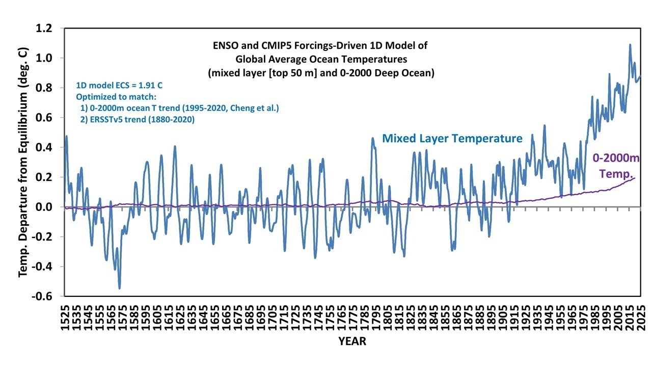
The following plot shows the 1D model-generated global average (60N-60S) mixed layer temperature variations after the model has been tuned to match the observed sea surface temperature temperature trend (1880-2020) and the 0-2000m deep-ocean temperature trend (Cheng et al., 2017 analysis data).

Note that the specified net radiative feedback parameter in the model corresponds to an equilibrium climate sensitivity of 1.91 deg. C. If the model was forced to match the SST observations during 1979-2020, the ECS was 2.3 deg. C. Variations from these values also occurred if I used HadSST1 or HadSST4 data to optimize the model parameters.
The ECS result also heavily depends upon the accuracy of the 0-2000 meter ocean temperature measurements, shown next.

The 1D model was optimized to match the 0-2000m temperature trend only since 1995, but we see in Fig. 2 that the limited data available back to 1940 also shows a reasonably good match.
Finally, here’s what the full 500 year model results look like. Again, the CMIP5 forcings begin only in 1765 (I assume zero before that), while the combined ENSO dataset begins in 1525.

Discussion
The simple 1D model is meant to explain a variety of temperature-related observations with a physically-based model with only a small number of assumptions. All of those assumptions can be faulted in one way or another, of course.
But the monthly correlation of 0.93 between the model and observed SST variations, 1979-2020, is very good (0.94 for 1940-2020) for it being such a simple model. Again, our primary purpose was to examine how observed ENSO activity affects our interpretation of warming trends in terms of human causation.
For example, ENSO can then be turned off in the model to see how it affects our interpretation of (and causes of) temperature trends over various time periods. Or, one can examine the affect of assuming some level of non-equilibrium of the climate system at the model initialization time.
If nothing else, the results in Fig. 3 might give us some idea of the ENSO-related SST variations for 300-400 years before anthropogenic forcings became significant, and how those variations affected temperature trends on various time scales. For if those naturally-induced temperature trend variations existed before, then they still exist today.
Just exactly what “significant” anthropogenic “forcings”?
Land use would be a biggie.
I think I understand the whole CAGWer phobia now: they’re afraid of change, which occurs constantly in a chaos system like a habitable planet (Earth) and they are even MORE afraid of it because they CANNOT control change.
Therefore, pointing out that change is a constant event on a habitable planet like ours, and even on non-habitable planets like Uranus and Saturn and Mars, terrifies them to pieces.
Sad.
Nice work, Dr. Roy. Any chance you could link to the temperature and forcing data as used?
Also, good estimate of the mixed layer depth, especially for the tropics …
All the best,
w.
And we waste billions of scarce research dollars funding all the many Cargo-cult Climate super computer computer GCM’s because……?????
A: It’s a Yobs program for B-grade physics PhDs and software engineers who like the government dole.
… tonnes easier than actually working in industry to have to actually produice something useful.
Work? What’s that?
Why is the coldest part of the Dalton Minimum 1807-1817 showing colder, when there was a doubling of El Nino episode frequency then? The same for the 1550-1585, El Nino conditions normally increase during centennial solar minima.
The post 1995 rise in the upper 2000 meters OHC is in part associated with low solar driving a warm AMO phase and reducing low cloud cover.
I see the rise in Temperature Departure from Equilibrium in Figure 3 starting at about 1915. However, this looks like the rise in temperatures as the Earth came out of the Little Ice Age. Where is the anthropogenic warming signal?
Oh boy, another tunable model.
A famous quote by John von Neumann as recalled by his friend:
I remember my friend Johnny von Neumann used to say, with four parameters I can fit an elephant, and with five I can make him wiggle his trunk.
How many parameters in your model?
Jerry
Ex falso, quodlibet.
This is one of the main fallacies of climastrology. There are plenty, climastrology denies logic and physics with all its might.
For example, count how may times the ‘equilibrium’ assumption is used even in a simple 1D model (also false assumption, the world is not 1D and essential features are missing with an 1D model, for example the horizontal energy transport).
Every time equilibrium is assumed in such a case, it is a false assumption. An assumption that would require action-at-distance/instant communication, which is denial of physics.
The most significant parameter for predicting the future is the net radiative feedback parameter which “corresponds to an equilibrium climate sensitivity (ECS) of 1.91 deg. C”. What does that mean? It means that there is no impending climate crisis. Anthropogenic warming will be slow and constrained. There is no evidence for large positive non-linear feedbacks in the SST. It’s similar to other recent estimates for the ECS derived from atmospheric temperature measurements. Another nail in the coffin for extremely large values for ECS used by some climate Alarmists in their (discredited) models.
Who calibrated thermometers to a 0.01 degree accuracy in 1525? Who created the dataset of worldwide sea temperatures at depths of 50 and 2000 meters back in 1525 to when a temperature was actually measured and large is the dataset?? To use the term “global” would seem to require data collected from thousands of collection points with highly skilled operators using calibrated (regularly) instruments otherwise this all just conjecture…
yes, its highly speculative to model a global sea temperature using data that did not exist in any form for much of the period. A tiny number of sea temperatures were plotted by HMS challenger back in the 1850’s but other than that we have no idea.
I reconstructed CET back beyond the usual 1659 start date using hundreds of records
It is interesting to see that upward twist in the 1530’s which does match the SST in Roys graphic and my belief is that we had a period around as warm as now for the period from 1470 to 1540 or so. of course sea temperatures are far less volatile than land temperatures but that rise around the 1540’s is interesting as is the subsequent dip to one of the coldest periods of the LIA
tonyb
Three oceans straddling the equator separated by land masses and shallow water but a common maximum temperature. Surely that gives a clear picture that there is a maximum ocean surface temperature:
https://1drv.ms/b/s!Aq1iAj8Yo7jNhAeQGp_7ns2Kulo9
The surface temperature is not the result of some delicate energy balance upset by trivial amounts of radiative gases. It is the consequence of extraordinarily powerful atmospheric processes that drive cloudburst and are strongly temperature dependent. The atmosphere changes gear when TPW reaches 30mm to create a level of free convection and goes into high gear when TPW reaches 38mm, to enable daily cloudburst.
Open ocean surface simple cannot exceed 32C on planet Earth. The physics of the atmosphere prevent it. Shutters start going up at 26C and are shut so tight by 28.5C that the energy uptake begins to decline even under the tropical sun:
https://1drv.ms/b/s!Aq1iAj8Yo7jNg3vzCCr-yZNwAEVd
Average surface temperature of 288K is also the arithmetic average of the two extremes 271.3K at the low end and 305K at the top – no “Greenhouse Effect” needed.
If you see a temperature trend over decades then look for the flaws in the measurement system. Earth’s thermostat is working fine as the moored tropical buoys verify for the Nino34 region:
https://1drv.ms/b/s!Aq1iAj8Yo7jNg3j-MHBpf4wRGuhf
It is worth noting that all climate models are forecasting a physical impossibility, showing the ocean surface temperature exceeding 32C; will not happen because it cannot happen.
The only connected ocean water surface that regularly exceeds 32C is found in the Persian Gulf. Uniquely, it is the only tropical or sub-tropical water above 10 degrees latitude and 28C that has not experienced a tropical cyclone in recorded history. It has recorded cloudburst on the southern and southwestern shore but they are rare. The prevailing northerly winds prevent the development of convective available potential energy that is essential to cloudburst and spinning up cyclones.
Cyclones are the supercharged energy rejection process. They can persist for days to weeks covering a wide path across large distances, cooling the surface below in their wake by up to 3 degrees C. Then dumping massive amounts of water, all the latent energy extracted from the ocean surface.
We’ve got to do something!
Superb
Isn’t this what we would expect to see given the Modern Solar Maximum?
Nelson December 11, 2020 at 9:16 pm
Modern solar maximum? Sunspot numbers have been dropping for a half century or more.
People keep claiming that “It’s the Sun, stupid” … so why is solar decreasing and temperatures increasing???
w.
30 years is meant to be “climate”…
If you take the 30 year trailing average of Greg Kopp’s TSI data you get the following
Solar energy is still very much near its highest in a long time.
Why on earth would you use a 30 year average? That’s an artificial human construct with nothing to do with TSI or its effects. TSI knows nothing of averages.
And even if we were to do that, it’s STILL not increasing. The 30-yr average has been dropping since 1984.
Regards,
w.
PS—I have no idea who “Greg Kopp” is. I use the TSI values from Leif Svalgaard, a solar scientist with a solar-related phenomenon named after him (the Svalgaard-Mansurov Effect).
Its all to do with ACCUMULATED ENERGY
Which is still very high.
Even Lief’s much adjusted data shows that.
Lief directed me to the data on Greg Kopps site.
Thanks for show the large accumulation of energy in the last 50-70 years 🙂
30 year trailing average? What has that got to do with anything?
As TSI is a derivative of sunspots, we are at a 100+ year low as defined by 4010 days average (11 year cycle) with an insignificantly lower reading around 1900.
(If you dig it up, you will be able to trace Greg Kopp’s TSI data back to https://agupubs.onlinelibrary.wiley.com/doi/full/10.1002/2016GL071866
“The nominal value of the TSI, averaged over Solar Cycle 23 (which lasted from 1996 to 2008), is 1361.0 ± 0.5 (W/m2), with a weak peak‐to‐peak solar cycle modulation of 0.08% that is in phase with the 11 year cycle [Kopp, 2016]. Assessing such tiny modulations requires not only high radiometric accuracy but also considerable care in the making of the composite record. ”
With:
“Here we concentrate on this methodology and introduce a novel, probabilistic approach that can be readily exported to other contexts. ”
And
The new TSI composite we obtain is not definitive because the original data still require some community‐endorsed corrections.
As well as referring to
http://www.issibern.ch/teams/solarirradiance/ for numbers,
http://www.issibern.ch/teams/solarirradiance/TSI_composite_DeWit.txt
; This is a preliminary version of the TSI, which is still pending
; decisions on the corrections to be made to the original data.
; Therefore this composite should not be used for publication.
; Two versions are provided: one based on the original instrument data,
; and one based on the same data, with corrections made by
; C. Froehlich on ACRIM1, ACRIM2, HF and ERBE
Models. All based on sunspots. Still not approved data going up to- and ending in 2015.
Oddgeir
So yes, Its the SUN,, Stupid !!
You put very large pot of water on and keep the heat near full, which it has been, it keeps warming.
Trump_Clone (fred250)
I see you are back to your Trump like tweets (comments), capitals and all.
Jerry
The strong solar cycles over the last 70 or so years have been heating the ocean, particularly the tropical oceans with the decrease in cloud cover. A lot of energy in a vast reservoir.
Before temperatures can cool, some of that energy build-up has to be released.
Not going to happen quickly, especially with the accumulated solar energy being so high for so long, as shown by TSI data.
Thinking that it should start cooling just because there has been one slightly lower solar cycle is very wobbly thinking.
Fred, TSI has been dropping steadily since it peaked in the late fifties, so I have no idea why you think there has been “one slightly lower solar cycle”.
w.
It is meaningless looking at sunspot numbers. The AMO changes inversely to the solar wind temperature/pressure. The AMO cooled in the 1970’s with the strongest solar wind states of the space age, and warmed from 1995 with the weakening of the solar wind since then. That’s why the North Atlantic is always warmer during centennial solar minima.
Odd that you don’t think the accumulated energy in the last 30 years is important.
Maybe use the last 40 years ?
Accumulated energy is what is stored in the oceans.
Willis,
While the level of sunspot activity has recently declined, it has declined from an unusually high level. Read “Unusual activity of the Sun during recent decades compared to the previous 11,000 years” in Nature, published in 2004.
https://www.nature.com/articles/nature02995
Here’s a quote from the abstract;
“According to our reconstruction, the level of solar activity during the past 70 years is exceptional, and the previous period of equally high activity occurred more than 8,000 years ago. We find that during the past 11,400 years the Sun spent only of the order of 10% of the time at a similarly high level of magnetic activity and almost all of the earlier high-activity periods were shorter than the present episode.”
An ‘ocean lag’ should show, like paleo-archives suggest. Measured in decades, not just years (like many grand-minimum watchers seem to hope), it’s at the core of the war so to speak. Its length could still vary, from 2- >5 or so it seems, so its more precise ocean mechanism could well be explained – how and why.
Willis, you need to take a longer perspective. You should have shown the graph for the entire sun spot record. Sunspots drive ocean heat content as SW radiation from the sun is highest during active cycles. Just because sunspot count is declining doesn’t mean SW radiation entering the ocean isn’t above a long term average. Dave Evans has some interesting work on a Notch Delay model that predicts a lag in response to changing SS numbers.
What I find weird is the lack of discussion of Holocene temperature variations. It seems to me that there are 2 possible explanations: internal variability of the system or solar. Of course, you can’t really seperate the two.
Willis. I’d be curious how you would explain the RWP and MWP. It seems logical to me that whatever caused those is likely responsible for the current warming
Nelson December 12, 2020 at 5:51 am
You have no evidence of that, and I’ve looked for a decade for evidence of that without finding any.
We went through Dave Evan’s “notch theory” in great detail here on WUWT. It’s a joke.
And you do understand that the 24/7 average global change in TSI between solar max and solar min is only about 0.15 W/m2? And by the time that gets past cloud and surface reflections it’s down to about half of that? And that that is in a system with 24/7 average downwelling radiation of half a kilowatt?
You are seriously claiming that a transient change of A TENTH OF ONE PERCENT in incoming energy in a hugely complex system will be detectable? Really? Because I cannot think of any natural system where that is true. That’s like saying if you add a cup of water to a stream you’ll see the effects a mile downstream … never gonna happen.
To start with, we still have no agreement on the variations in Holocene temperature. Various authors say various things, including Michael Mann …
Next, neither I nor anyone else understands the climate to that level. Nobody knows why the MWP started and ended when it did. No one knows why there was a Little Ice Age. No one knows why we haven’t gone into a real glaciation, why the LIA ended when it did, or why we’ve been warming for three centuries since the Little Ice Age (can’t be CO2, the CO2 rise started far too late to explain it).
And those are among the reasons I just laugh when “scientists” claim they know what the climate in 2050 will be like. We can’t explain the past, but we can predict the future?? Say what?
In closing, Nelson, I’ve looked in more places for the signature of solar sunspot-related variations than anyone I know. I can find no effect which is visible on the surface. Yes, sunspots do affect the ionosphere … but I cannot find any evidence that it makes it all the way down to the surface.
There’s a partial list of my investigations into this question here. Please read them ALL if you wish to continue this interesting discussion.
w.
PS—The discussion of the bogus notch-delay model is here, here, and here.
Willis:
You said “Nobody knows why the MWP started and ended when it did”
I KNOW, and you should, too, since I have previously explained the reason to you.
Burl Henry December 12, 2020 at 11:29 am
I fear I have no memory of this, so a link would be useful. Don’t try to tell us it was volcanoes, though. I discussed that incorrect argument in Dronning Maud Meets The Little Ice Age.
Best regards,
w.
Willis:
You asked for a link:
It is your “Watts Available” Guest Essay of Sept. 23, where I debunked your “Drowning Maud…” essay in my post of Oct. 2, 2020, 7:56 pm).
Your essay is seriously flawed, which led you to the wrong conclusion, that SO2 was not responsible for the periods of increased ice growth.
I would refer you again to my paper”Experimental Proof that Carbon Dioxide does NOT cause global warming”
http://www.scholink.org/ojs/index.php/se/
The Table in that paper shows that anomalous temperature increases of ~ 0.2 deg. C occur during each recession, due to decreased SO2 aerosol emissions (in the range of 0.3-1 Megatons, depending upon the length of the recession).
For comparison, the average amount of SO2 emitted from 36 VEI4 eruptions since 1979 is 0.5 Megatons (satellite measurements). When their SO2 settles out, anomalous temperatures rise to pre-eruption levels (an increase of ~ 0.2 deg C).
I have since plotted the anomalous temperature data since 1850 – present, and EVERY temporary temperature increase is due to decreased levels of SO2 in the atmosphere, and EVERY temperature decrease is due to increased SO2 in the atmosphere, primarily from VEI4 eruptions).
Your conclusion that SO2 from VEi4 eruptions has no climatic effect is 100% wrong. As was also shown in my analysis of the Central England Instrumental Temperature Data Set,1659-present which you have viewed https://www.osf.io/b2vxp/
Willis, I would bet that you believe that sunlight provides most of the ocean heat content and that its the SW part that matters most? My point about the Notch Delay theory (And I read through Lubos Molt’s critic years ago) was just to point out that there are long and variable lags in the relationship between heat entering the ocean and how that heat might effect the earth’s climate. I don’t think we disagree that cycle to cycle, sun spots don’t explain much of anything about observed temperatures. However, the distribution of heat in the oceans and how that heat get released through time matters to climate.
I believe the general evidence of climate change during the Holocene, especially since the RWP, are fairly clear, though all proxies are measured with error. In fact, the RWP, the Dark Ages, the MWP, the LIA are well documented in written history, art work, agricultural data, as well as a long list of proxies.
I agree that we don’t understand climate well enough, However, there is a fairly short list of explanations. I am willing to believe its just internal variability of a complex system. I am also willing to believe there are long term changes in solar output, not just cycle to cycle changes. One thing is fairly clear, none of the changes can be explained by CO2 dynamics. I agree that trying to make prediction about what will happen the next 50 to 100 years makes little sense if we can’t explain the variation shown in the data from the last few thousand years.
Willis, would you agree that orbital dynamics, which leads to changes in insolation, drive the glacial/interglacial cycle during the Pleistocene. If so, isn’t this an admission that the sun (meaning the changes in insolation at say 65 north, even if solar output is constant) drives observed climate over time.
Nelson December 12, 2020 at 2:56 pm
Nope.
w.
Hi Willis,
Suppose I could show that a tenth of a percent change in the total heating in the tropics could make a major change in the vertical velocity of mesoscale storms in that region. Would that surprise you?
Jerry
Willis,
Have you looked at the manuscript byKopp et al. titled
Total solar irradiance data record accuracy and consistencyimprovements.
The variation between instruments is revealing, but all of the instruments do show a direct correspondence between sunspot activity and TSI. The adjusted results barely show an accuracy of a tenth of a percent so if that is significant (as I think I can show),
then wouldn’t that mean there would be decadal impacts on the climate?
And another article stated that there has been a increase of .05% in TSI during solar mins per decade since 1970, i.e. the sun is getting hotter.
Jerry
Gerald Browning December 13, 2020 at 1:40 pm
Total heating in the tropics is 633 W/m2. A tenth of a percent of that is 0.63 W/m2.
However, as I’ve demostrated over and over, the threshold for deep convection is temperature based. It is NOT forcing based.
So if that change warms the surface to a level above that threshold, it could indeed make a difference. That’s the thing about thresholds—once you pass them, the new emergent phenomena can present themselves very rapidly.
However, that’s certainly not going to happen everywhere. And there’s no guarantee it will make any difference, it may get lost in the noise.
w.
Gerald Browning December 13, 2020 at 2:16 pm Edit
Yes, although it was years ago.
Not enough information to answer. However, don’t forget that TSI only varies by ~ 0.15 from trough to peak and spends most of its time in the midrange.
In addition, of the ~ 340 W/m2 at the top of the atmosphere, only 164 W/m2 are absorbed by the surface. So only ~ half of the 0.15 W/m2, 0.07 W/m2, is making it to the surface.
CERES data says no. It shows a drop of 0.02 W/m2 from 2000 to 2019. This agrees with the SILSO data, which drops in that same time period. And the SILSO data is not single-trended, it goes up and down over time.
w.
Jerry
“why is solar decreasing and temperatures increasing???”
Maybe for the same reason why a pot of water still can boil even if you decrease the flame under it a bit.
Climastrologers would expect it to freeze instantly the moment you decrease the flame a little, but the water, despite their blind religious belief, can still warm up to boiling.
Nope. Makes no sense.
w.
If CO2 is the control knob to temperature then how come the 0-2000 meter temperature drops starting around 1815? Did something eat all the CO2 out of the air? (Figure 3) And how come the 50 meter temperature goes up at the same time?
Something doesn’t “smell right” about the behavior during the little age age events.
I still belief there is “noise” in the ocean temperature measurements before modern use of buoys. They can correct for these all they want – their corrections are just more biased guesswork.
I like a simple model, but a model can’t produce meaningful results without meaningful data. I trust the “ocean temperature reconstruction” about as much as I trust Micheal Mann’s Tree-Proxy Land Temperature reconstruction. There are just too many variables in nature to simplify a reconstruction to one thing.
As opposed to Fig 2, Ago data shows no net change in global ocean temperatures 65 N – 65 S 0 -1900m from 2004 – 2013:
Here is a similar story for the SST based on Aqua/MODIS data for almost the same time period but presented as a difference over the period across longitudinal bands:
https://1drv.ms/u/s!Aq1iAj8Yo7jNg3GJZzfUccCa6osu
The cooling above 55N is also evident on the surface.
The area averaged SST has declined slightly based on the Aqua/MODIS data. However the equatorial SST has not changed over the 2 decades.
It all makes the case that Earth’s thermostat is doing a fine job; tighter control than most industrial control systems.
Chris Hanley wrote:
“As opposed to Fig 2, Ago data shows no net change in global ocean temperatures 65 N – 65 S 0 -1900m from 2004 – 2013:”
Perhaps I am reading it incorrectly, but I see the following:
– Your plots from Argo indicate a warming of about 0.02K (or perhaps 0.03K) between 2004 and 2020
– Dr. Spencer’s plots indicate a warming of about 0.06K between 2004 and 2020
In other words, Your chart of Argo (adjusted) measurement data *also* shows some warming, but about 1/3 (or 1/2) that shown by Dr. Spencer.
Looking at it again, it looks like the Argo data indicates 0.04K of warming between 2004 and 2020 and about 0.05K of warming between 2005 and 2020. That’s only a bit less than that shown in Dr. Spencer’s plot.
Since the uncertainty interval for the Argo floats is about +/- 0.5C how can you determine a difference of temperature in the hundredths digit?0.06K, 0.04K, 0.03K, 0.02K, 0.01K are all within the uncertainty interval, meaning you don’t actually know if differences that small actually exist.
An italian group did an interesting experiment over a perion of several years. Apparently there is an are in italy that is ouzing pure CO² (1.000.000ppm) into the atmosphere so that put a ballon on it and allowed the sun to heat it. They did the same with atmospheric gas and found a difference in cooling of 1.3C
They absolutely would Stephen – depending on the ‘colour’ of their balloon and its effective albedo.
BECAUSE.#: CO2 has very very low emissivity
Thee balloon stops convection, the surrounding air has very low thermal conductivity as we all know so that, depending on what I said above, the only way the balloon could lose heat was by radiating it away.
(It was made of stuff fairly transparent to 10 micron wavelengths?)
Do NOT EVER assume that because me or you sees something/anything as being ‘black’ that it is black across the entire electromagnetic spectrum.
U iz in 4A shok!!
Because the CO2 emissivity is 10% that of atmospheric air, the gas in the balloon *had* to heat up
Jozef Stefan put a thin metal plate (a Lamella) in a ‘balloon’ and got a temperature of over 1,900 Celsius when exposed to El Sol
That’s how he worked out the temperature of Old El Sol
There’s some homework for us all………..
Roy,
I have looked a lot at CMIP5 models and the forcings. The question I have with your analysis is what the correlation is if you subtract the smooth prior (ie the CMIP5 model forcings, calibrated by linear regression to the temperature series) from your 1D simulation and from the temperature series.
The reason is that there is a fundamental question mark in my mind over the models. They are almost entirely dependent on the prior (ie the forcings). I am not convinced they add anything other than that. For example:
1. I can obtain a correlation with HadCrut4 temp series as good as the CMIP5 model mean (R=0.92) by just trivially using linear regression of the input forcings grouped into just two series – sum of natural and the sum of the Anthropogenic components with an optimised lag for each.
2. The same linear regression model has a correlation with the CMIP5 model mean of 0.98
3. If I subtract the CMIP5 model mean of the basic set of 39 climate models (KNMI) from each climate model output the residuals of the climate models are uncorrelated random noise and have almost no correlation with the temp residuals calculated in the same way.
In other words, the only reason the climate model output fit the temp series so well is because the input prior forcings fit the temperature series. The climate model themselves add very little predictive value or insight as far as I can see (this is a common misunderstanding of the role of the low frequency prior in my own field of seismic inversion for earth impedance).
In your case you are trying to model the Enso response. So the correct comparison is to subtract the model mean from both your output and the temp series and look at the fit of the residuals. Otherwise your high apparent correlation is largely the product of the forcings, not of your ENSO modelling.
Unless I misunderstood something in your method.
Sorry but I see 2 main problems here.
1) just as in the ‘Saturation’ essay we endured recently, we see here the epic overuse of the term Radiative Forcing
Its quite obvious in both cases that the authors have NO REAL IDEA what they are talking about and that the repeated use of the term(s) will bludgeon some sort of understanding into the readers.
The Human Animal cannot lie – it ALWAYS gives itself away somehow.
Basically: Intimidation meets the Emperor’s New Wardrobe master
2) Absolutely Fundamental and an appeal to the authority of the guy Warmists appeal to. Jozef Stefan
Stefan said, in the rather obscure scientific language of his time that: (You had to be fairly bright, clever and alert of understand it and patently nobody is these days)
Stefan said:
“An object, any object and all objects with a temperature other than zero Kelvin radiate energy according to their temperature AND their emissivity.”
(Nobody these days wants to know about emissivity – is it sounding too much like emissions? sigh)
He continued by saying that it matters NOT what other objects are near or far, what *their* temperatures are or what the are made or anything about them in ANY WAY mattered.
Now do you see The fail in the Green House Gas Effect? (GHGE)
It completely trashes what he said there and DO remember, Stefan is The Authority this entire debacle is based upon
Because the GHGE says that the radiation leaving the Earth’s surface (soil, dirt, water etc) IS dependant upon not only the temperature of the atmosphere but most crucially, what it is made of.
Please do try get your head around that. FORGET what you (imagine you) know about ‘feedback
Even before the Thermodynamic Insanity which says that radiations from cold objects are absorbed by warm ones.
DO NOT worry about The Energy (conservation).
It will slip slide its way out of anywhere
We are in the midst of Complete Madness and it only seems to get worse almost daily
Lets have 100% CO2 at 15 Celsius (288K) and one bar pressure.
It will be radiating 0.78 watts per square metre
But atmospheric CO2 is only 400ppm, so the power coming from what we’ve got now will be 312 micro watts per square metre
If we took the average temp of the atmosphere to be minus 15C and 400ppm we get: 200 micro Watts
And that the CO2 is actually radiating at 15 micron or minus 79 C:
=64 micro watts per square metre
We see now why *nobody* has yet actually measured this hideous Climate Destroying Climate Radiative Feedback Forcing
It makes the stability of El Sol, graphed by Willis here, look like a gang of drunken teenagers, in a trainwreck while falling of a cliff onto a trampoline.
During an earthquake
Peta of Newark December 12, 2020 at 4:35 am
I’m sorry, but flat definitive statements like “the authors have no real what they are talking about” are MEANINGLESS. All that is is your own private opinion, and on a scientific site, the unsupported opinion of some random anonymous popup is a total waste of electrons.
w.
Willis,
Did you see my comment above? Have you read the manuscript by Kopp et al. entitled
Total solar irradiance data record accuracy and consistency improvements
The graphs show a definite correlation between sunspot number and TSI. Also note the difference
between platforms and the way they were adjusted to be closer to each other. And lastly
note the accuracy errors. It appears that the measurement error can be around .1%?
If my statement above is correct, then that is the range that can make a difference in how equatorial meso scale storms behave.
Willis,
In the midlatitudes when you change from the large scale (~1000 km) to the mesoscale
(100 km) the nondimensional forcing (H = total heating+cooling) goes from being O(1) to O(10) in the nondimensional potential temperature (or entropy) equation. What that means is that the vertical velocity must be directly proportional to H in mesoscale storms (see our 2002 manuscript). The main reason for the difference is that the pressure perturbation on the mean is a factor of 10 smaller in mesoscale storms. As you move toward the equator, the pressure perturbations on the mean are also smaller so small changes in H on the order of .1%
cause a similar balance between the vertical velocity and H. If this is the case (I will recheck the scaling to verify this),then changes in the TSI of that order can make a substantial difference in the behavior of smaller scale storms in near the equator.
Jerry
Gerry, if that were true we should see some sign of it in some surface dataset … but I’ve never found it despite much looking.
Where would you think we might find it? The effect of sunspots on TSI is well-known, as is the relationship between sunspots and radio correlation because of the effect on the ionosphere. But where is the effect of sunspots on mesoscale storms?
Point me to the dataset, I’m happy to take a look.
w.
Willis,
What is the clear sky solar radiation difference (watts per square meter) at the tropic of cancer between the summer and winter solstice? It seems a fairly straight forward question but I cannot find the answer.
Jerry
Jerry, the CERES data gives me the following for the clear-sky downwelling solar at the surface at the Tropic of Cancer.
Maximum downwelling: 328.6 W/m2
Minimum downwelling: 188.8 W/m2
These are 24-hour averages. Peak values would be 4x that.
w.
Willis,
Compared to the TSI
328.6/1360=.24
188.8/1360=.14
that means only 24% to 14 % reaches the surface on a clear day at the Tropic of Cancer
during these two periods.
So a 54% change [ (328.6−188.8)/(.5*(328.6+188.8)) =.54 ] at the surface is sufficient to
move the ITCZ if the skies were clear.
How do these numbers differ when the sky is cloudy, e.g., if the ITCZ is were in the way?
Might I ask how reliable do you feel the clear sky numbers are and those with cloudiness?
Jerry
Jerry, let me back up a minute.
The ITCZ generally follows the sun, as you might expect. However, it rarely goes north of 15°N or 15° S. So it’s not clear what you mean when you say that the difference in temperature “is sufficient to move the ITCZ if the skies were clear”.
I mean, how is this different from any year? And what is the end game? What are you trying to establish or falsify?
Best regards, thanks for the interesting discussion,
w.
Hi Willis,
If in clear skies only 14% to 24% of TSI reaches the surface at the Tropic of Cancer at minimum and maximum times, how much reaches the surface in cloudy times at the ITCZ? I am guessing it is much less and that the amount is not a well known number?
Jerry
Jerry, the problem is when you divide by 1360. That’s instantaneous TSI. But you have to use the 24/7 average TOA solar, which at the Tropic of Cancer is 464 W/m2
Also, that’s just at summer solstice. At winter solstice the Tropic of Cancer is only getting 274 W/m2 because of the angle it’s hitting the earth at.
As a result, at summer solstice some 329/464 = 71% of the sunshine making it to the ground.
And at winter solstice, as you’d imagine in the tropics without a real summer or winter, it’s about the same at 189/274 = 69%.
Hope this helps with your calcs,
w.
Willis,
Now I am really confused. Why use 24/7 values when only half of the earth is in sunlight . Then the value would be much less than in the day? And why do they use instantaneous values for TSI given the same reasoning? It seems like comparing apples to oranges?
Jerry
It’s divided by 4 because it’s the difference between a globe and a circle. The surface of one is pi r2, the surface of the other is 4 * pi r2
w.
Willis,
After a bit of checking, I will ask what is the daily solar irradiation in clear skies at the surface at the Tropic of Cancer during the summer and winter solstice and what is it under cloudly skies, e.g. under the ITCZ?
Jerry
Gerald Browning December 16, 2020 at 11:00 am
I can give you clear and cloudy … but the ITCZ rarely gets that far north. And clear and cloudy likely refer to different locations as well as different conditions.
And any analysis of the Tropic of Cancer includes both cloudy and clear areas, see below.
w.
Hi Willis,
Thanks for your patience.
Choose any clear area in the Tropic of Cancer during the two solstices. That gives me a feel
for the difference in solar irradiation during the minimum and maximum times.
Are these measurements from surface instruments or satellite?
And (if possible) the solar irradiation under a storm in the ITCZ.
Jerry
Gerald Browning says:
December 16, 2020 at 9:58 pm
Can do, give me a couple days.
The measurements are from the CERES EBAF satellite-based dataset. Description of their processes is here.
Finally, solar under a storm … I do not have daily data, just monthly, so I can’t say what it’s like under a storm.
w.
Willis,
Are there any ground based obs to check the satelite measurements? Isn’t it the case that the satellites have problems in cloudy areas such as the ITCZ?
Gerald, the processing of the info for the CERES dataset is here. Another is here.
Man I HATE THIS NEW WUWT FORMAT!!
Why can’t I post a damn link directly?
w.
Willis,
Can you reply to my email so we can correspond directly.
I would like to discuss in more detail where I am coming from.
Jerry
Willis,
The two numbers from your routine are both about 10% apart (or less if you use the larger number in the denominator). So am I correct
in stating the difference between the solstices is about a 10%
solar irradiation?
Am I reading your routine correctly that is does not take in any outside data, i.e., satelite data?
Jerry
Also, Jerry, you can calculate clear-sky irradiation from some data. I program in R, here’s the function:
insolation(zenith, jd, height, visibility, RH, tempK, O3, alphag)
ARGUMENTSzenith Zenith angle in degrees.jd Julian Day.height Altitude above sea level.visibility Visibility [km].RH Relative humidity [%]tempK Air temperature [K]O3 Ozone thickness [m]alphag Albedo of the surrounding terrain [0 to 1].So for the two conditions we have:Summer Solstice:insolation(0, 2457561, 0, 28, 60, 278.15, 0.003, 0.2)In Id888.0739 182.3656where In is direct and Id is diffuse solar energy. Here's the winter condition:insolation(2*23.45, 2457744, 0, 28, 60, 278.15, 0.003, 0.2)In Id813.2435 165.8305Finally, here's the guts of the function. "nargs" is the number of argumentsfunction (zenith, jd, height, visibility, RH, tempK, O3, alphag)
{
if (nargs() < 8) {
cat(“USAGE: insolation(zenith,jd,height,visibility,RH,tempK,O3,alphag)”)
return()
}
if (min(tempK, na.rm = TRUE) < 153) {
print(“temperature should be in Kelvin”)
return()
}
Isc = 1361.8
theta = radians(zenith)
ssctalb = 0.9
Fc = 0.84
Pz = z2p(height)
Mr = 1/(cos(theta) + 0.15 * ((93.885 – zenith)^(-1.253)))
Ma = Mr * Pz/1013.25
wvap_s = wvapsat(tempK)
Wprec = 46.5 * (RH/100) * wvap_s/tempK
rho2 = sunr(jd)
TauR = exp((-0.0903 * (Ma^0.84)) * (1 + Ma – (Ma^1.01)))
TauO = 1 – ((0.1611 * (O3 * Mr) * (1 + 139.48 * (O3 * Mr))^(-0.3035)) –
0.002715 * (O3 * Mr) * (1 + 0.044 * (O3 * Mr) + 3e-04 *
(O3 * Mr)^2)^(-1))
TauG = exp(-0.0127 * (Ma^0.26))
TauW = 1 – 2.4959 * (Wprec * Mr) * ((1 + 79.034 * (Wprec *
Mr))^0.6828 + 6.385 * (Wprec * Mr))^(-1)
TauA = (0.97 – 1.265 * (visibility^(-0.66)))^(Ma^0.9)
TauTotal = TauR * TauO * TauG * TauW * TauA
In = 0.9751 * (1/rho2) * Isc * TauTotal
tauaa = 1 – (1 – ssctalb) * (1 – Ma + Ma^1.06) * (1 – TauA)
Idr = 0.79 * (1/rho2) * Isc * cos(theta) * TauO * TauG *
TauW * tauaa * 0.5 * (1 – TauR)/(1 – Ma + Ma^(1.02))
tauas = (TauA)/tauaa
Ida = 0.79 * (1/rho2) * Isc * cos(theta) * TauO * TauG *
TauW * tauaa * Fc * (1 – tauas)/(1 – Ma + Ma^1.02)
alpha_atmos = 0.0685 + (1 – Fc) * (1 – tauas)
Idm = (In * cos(theta) + Idr + Ida) * alphag * alpha_atmos/(1 –
alphag * alpha_atmos)
Id = Idr + Ida + Idm
In[zenith > 90] = 0
Id[zenith > 90] = 0
return(cbind(In, Id))
}
Hope this helps.w.Willis,
I though you might not see my comment so repeated the question. Sorry.
Jerry
I note that, according to Fig. 3, the temperature was 0.5 above equilibrium in 1525. Temperature, 500 years later in 2025 is expected to be 0.9 above equilibrium. Not sure what all the shouting is about.
The calculated El Nino and La Nina peaks seem to fit very well the observations. I have used the same empirical relationship as Trenberth et al. that the temperature impact of ENSO event is 0.1 * ONI and there is 6 months delay. It works equally well. Otherwise, ENSO effects have nothing to do with global warming; there is no long-term trend.
There is no model, which could predict the frequency and magnitude of ENSO events. I have found out that during two super El Ninos 1997-98 and 2015-16 positive shortwave anomalies caused slightly more than 50 % of the global temperature responses.
I am wondering that Dr. Spencer has been used ECS values: “If the model was forced to match the SST observations during 1979-2020, the ECS was 2.3 degrees.” ECS happens in the century-scale and TCS-models reacts in the timespan of one year or more.
A simple SST model would only really be relevant to the Southern Hemisphere
If applied to the NH above 45º does it show a clear war period around the 1930s/40s being similar to now?