guest post by Nick Stokes
There has been a lot of discussion lately of error propagation in climate models, eg here and here. I have spent much of my professional life in computational fluid dynamics, dealing with exactly that problem. GCM’s are a special kind of CFD, and both are applications of the numerical solution of differential equations (DEs). Propagation of error in DE’s is a central concern. It is usually described under the heading of instability, which is what happens when errors grow rapidly, usually due to a design fault in the program.
So first I should say what error means here. It is just a discrepancy between a number that arises in the calculation, and what you believe is the true number. It doesn’t matter for DE solution why you think it is wrong; all that matters is what the iterative calculation then does with the difference. That is the propagation of error.
A general linear equation in time can be formulated as
y’ = A(t)*y+f(t) ……….(1)
y(t) could be just one variable or a large vector (as in GCMs); A(t) will be a corresponding matrix, and f(t) could be some external driver, or a set of perturbations (error). The y’ means time derivative. With a non-linear system such as Navier-Stokes, A could be a function of y, but this dependence is small locally (in space and time) for a region; the basics of error propagation follow from the linearised version.
I’ll start with some bits of DE theory that you can skip (I’ll get more specific soon). If you have another solution z which is the solution following an error, then the difference satisfies
(y-z)’=A*(y-z)
The dependence on f(t) has gone. Error propagation is determined by the homogeneous part y’=A*y.
You can write down the solutions of this equation explicitly:
y(t) = W(t)*a, W(t) = exp(∫ A(u) du )
where the exp() is in general a matrix exponential, and the integral is from starting time 0 to t. Then a is a vector representing the initial state, where the error will appear, and the exponential determines how it is propagated.
You can get a long way by just analysing a single error, because the system is linear and instances can be added (superposed). But what if there is a string of sequential errors? That corresponds to the original inhomogeneous equation, where f(t) is some kind of random variable. So then we would like a solution of the inhomogeneous equation. This is
y(t) = W(t) ∫ W-1(u) f(u) du, where W(t)=exp(∫ A(v) dv ), and integrals are from 0 to t
To get the general solution, you can add any solution of the homogeneous equation.
For the particular case where A=0, W is the identity, and the solution is a random walk. But only in that particular case. Generally, it is something very different. I’ll describe some special cases, in one or few variable. In each case I show a plot with a solution in black, a perturbed solution in red, and a few random solutions in pale grey for context.
Special case 1: y’=0

This is the simplest differential equation you can have. It says no change; everything stays constant. Every error you make continues in the solution, but doesn’t grow or shrink. It is of interest, though, in that if you keep making errors, the result is a random walk.
Special case 2: y”=0

The case of no acceleration. Now if there is an error in the velocity, the error in location will keep growing. Already different, and already the simple random walk solution for successive errors doesn’t work. The steps of the walk would expand with time.
Special case 3: y’=c*y
where c is a constant. If c>0, the solutions are growing exponentials. The errors are also solutions, so they grow exponentially. This is a case very important to DE practice, because it is the mode of instability. For truly linear equations the errors increase in proportion to the solution, and so maybe don’t matter much. But for CFD it is usually a blow-up.

But there are simplifications, too. For the case of continuous errors, the earlier ones have grown a lot by the time the later ones get started, and really are the only ones that count. So it loses the character of random walk, because of the skewed weighting.
If c<0, the situation is reversed (in fact, it corresponds to above with time reversed). Both the solutions and the errors diminish. For continuously created errors, this has a kind of reverse simplifying effect. Only the most recent errors count. But if they do not reduce in magnitude while the solutions do, then they will overwhelm the solutions, not because of growing, but just starting big. That is why you couldn’t calculate a diminishing solution in fixed point arithmetic, for example.
This special case is important, because it corresponds to the behaviour of eigenvalues in the general solution matrix W. A single positive eigenvalue of A can produce growing solutions which, started from any error, will grow and become dominant. Conversely the many solutions that correspond to negative eigenvalues will diminish and have no continuing effect.
Special case 4: Non-linear y’=1-y2
Just looking at linear equations gives an oversimplified view where errors and solutions change in proportion. The solutions of this equation are the functions tanh(t+a) and coth(t+a), for arbitrary a. They tend to 1 as t→∞ and to -1 as t→-∞. Convergence is exponential. So an error made near t=-1 will grow rapidly for a while, then plateau, then diminish, eventually rapidly and to zero.

Special case 5: the Lorenz butterfly
This is the poster child for vigorous error propagation. It leads to chaos, which I’ll say more about. But there is a lot to be learnt from analysis. I have written about the Lorenz attractor here and in posts linked there. At that link you can see a gadget that will allow you to generate trajectories from arbitrary start points and finish times, and to see the results in 3D using webGL. A typical view is like this

Lorenz derived his equations to represent a very simple climate model. They are:

The parameters are conventionally σ=10, β=8/3, ρ=28. My view above is in the x-z plane and emphasises symmetry. There are three stationary points of the equations, 1 at (0,0,0),(a, a, 27)and,(-a, -a, 27) where a = sqrt(72). The last two are centres of the wings. Near the centres, the equations linearise to give a solution which is a logarithmic spiral. You can think of it as a version of y’=a*y, where a is complex with small positive real part. So trajectories spiral outward, and at this stage errors will propagate with exponential increase. I have shown the trajectories on the plot with rainbow colors, so you can see where the bands repeat, and how the colors gradually separate from each other. Paths near the wing but not on it are drawn rapidly toward the wing.
As the paths move away from the centres, the linear relation erodes, but really fails approaching z=0. Then the paths pass around that axis, also dipping towards z=0. This brings them into the region of attraction of the other wing, and they drop onto it. This is where much mixing occurs, because paths that were only moderately far apart fall onto very different bands of the log spiral of that wing. If one falls closer to the centre than the other, it will be several laps behind, and worse, velocities drop to zero toward the centre. Once on the other wing, paths gradually spiral outward toward z=0, and repeat.
Is chaos bad?
Is the Pope Catholic? you might ask. But chaos is not bad, and we live with it all the time. There is a lot of structure to the Lorenz attractor, and if you saw a whole lot of random points and paths sorting themselves out into this shape, I think you would marvel not at the chaos but the order.
In fact we deal with information in the absence of solution paths all the time. A shop functions perfectly well even though it can’t trace which coins came from which customer. More scientifically, think of a cylinder of gas molecules. Computationally, it is impossible to follow their paths. But we know a lot about gas behaviour, and can design efficient ICE’s, for example, without tracking molecules. In fact, we can infer almost everything we want to know from statistical mechanics that started with Maxwell/Boltzmann.
CFD embodies chaos, and it is part of the way it works. People normally think of turbulence there, but it would be chaotic even without it. CFD solutions quickly lose detailed memory of initial conditions, but that is a positive, because in practical flow we never knew them anyway. Real flow has the same feature as its computational analogue, as one would wish. If it did depend on initial conditions that we could never know, that would be a problem.
So you might do wind tunnel tests to determine lift and drag of a wing design. You never know initial conditions in tunnel or in flight but it doesn’t matter. In CFD you’d start with initial conditions, but they soon get forgotten. Just as well.
GCMs and chaos
GCMs are CFD and also cannot track paths. The same loss of initial information occurs on another scale. GCMs, operating as weather forecasts, can track the scale of things we call weather for a few days, but not further, for essentially the same reasons. But, like CFD, they can generate longer term solutions that represent the response to the balance of mass, momentum and energy over the same longer term. These are the climate solutions. Just as we can have a gas law which gives bulk properties of molecules that move in ways we can’t predict, so GCMs give information about climate with weather we can’t predict.
What is done in practice? Ensembles!
Analysis of error in CFD and GCMs is normally done to design for stability. It gets too complicated for quantitative tracing of error, and so a more rigorous and comprehensive solution is used, which is … just do it. If you want to know how a system responds to error, make one and see. In CFD, where a major source of error is the spatial discretisation, a common technique is to search for grid invariance. That is, solve with finer grids until refinement makes no difference.
With weather forecasting, a standard method is use of ensembles. If you are unsure of input values, try a range and see what range of output you get. And this is done with GCMs. Of course there the runs are costlier, and so they can’t do a full range of variations with each run. On the other hand, GCM’s are generally surveying the same climate future with just different scenarios. So any moderate degree of ensemble use will accumulate the necessary information.
Another thing to remember about ensemble use in GCM’s is this. You don’t have to worry about testing a million different possible errors. The reason is related to the loss of initial information. Very quickly one error starts to look pretty much like another. This is the filtering that results from the vary large eigenspace of modes that are damped by viscosity and other diffusion. It is only the effect of error on a quite small space of possible solutions that matters.
If you look at the KNMI CMIP 5 table of GCM results, you’ll see a whole lot of models, scenarios and result types. But if you look at the small number beside each radio button, it is the ensemble range. Sometimes it is only one – you don’t have to do an ensemble in every case. But very often it is 5,6 or even 10, just for 1 program. CMIP has a special notation for recording whether the ensembles are varying just initial conditions or some parameter.
Conclusion
Error propagation is very important in differential equations, and is very much a property of the equation. You can’t analyse without taking that into account. Fast growing errors are the main cause of instability, and must be attended to. The best way to test error propagation, if computing resources are adequate, is by an ensemble method, where a range of perturbations are made. This is done with earth models, both forecasting and climate.
Appendix – emulating GCMs
One criticised feature of Pat Frank’s paper was the use of a simplified equation (1) which was subjected to error analysis in place of the more complex GCMs. The justification given was that it emulated GCM solutions (actually an average). Is this OK?
Given a solution f(t) of a GCM, you can actually emulate it perfectly with a huge variety of DEs. For any coefficient matrix A(t), the equation
y’ = A*y + f’ – A*f
has y=f as a solution. A perfect emulator. But as I showed above, the error propagation is given by the homogeneous part y’ = A*y. And that could be anything at all, depending on choice of A. Sharing a common solution does not mean that two equations share error propagation. So it’s not OK.
Nick Stokes
Thanks Nick for the good exposé, but I miss here quite a lot of what you so pretty good explained on your own blog:
https://moyhu.blogspot.com/2019/09/how-errors-really-propagate-in.html
That was really amazing stuff.
Best regards
J.-P.
Thanks, Bindi
The problem is it is wrong from the first equation and gets more wrong every equation after that. This is the problem with Layman pretending to be scientists like Nick and Mosher and especially those of the old science variety.
Radiative transfer has it’s own version of system linear equations because of its quantum nature.
https://en.wikipedia.org/wiki/Quantum_algorithm_for_linear_systems_of_equations
There are any number of good primers on Quantum linear systems algorithms on university sites on the web.
Nicks basic claim is that his equations somehow covers the problem generally .. when any actual physicist knows for a fact that is a NOT EVEN WRONG.
I should also add Daniel Vaughan put up a good 3 part series on programming for quantum circuits on codeproject
https://www.codeproject.com/Articles/5155638/Quantum-Computation-Primer-Part-1
If you follow the basic mathematics you will understand how something linear in the Quantum domain gets very messy in the classical domain.
LdB is right. There was a study some time ago (https://news.ucar.edu/132629/big-data-project-explores-predictability-climate-conditions-years-advance reported on WUWT) in which climate models were re-run over just one decade with less than a trillionth(!) of a degree difference in initial temperatures. The reults differed hugely from the original run, with some regions’ temperatures changing by several degrees. NCAR/UCAR portrayed it as a demonstration of natural climate variabiliity. It wasn’t, of course, it was a demonstration of the instability of climate models.
As LdB says: The problem is it is wrong from the first equation and gets more wrong every equation after that.
“It wasn’t, of course, it was a demonstration of the instability of climate models.”
They aren’t unstable. They are just not determined by initial conditions. Same with CFD.
The initial conditions determined the wide variability in output. They may not be unstable but that doesn’t mean they don’t have huge uncertainty associated with their outputs.
You can determine all the start conditions you like if you it tells you nothing about the behaviour because it isn’t a classical system. Take a piece of meta-material engineered to create the “greenhouse effect” and you can know every condition your classical little measurements can muster you still won’t be able to predict what will happen using any classical analysis. The bottom of the problem is actually easy to understand temperature is not a fundamental statistic it is a made up classical concept with all the problems that goes with that.
They are unstable. They have code that purposely flattens out the temperature projections because they too often blew up. Modelers have admitted this. Also Nick you said :
“It is just a discrepancy between a number that arises in the calculation, and what you believe is the true number.” THAT IS WRONG. What you believe is not important. What is important is the true number that is backed up by observations that you obtain by running real world experiments.
There is no essential difference between an error of 0.000000001 deg C in the initial conditions and a 0.000000001 deg C error in the first few iterations (typically 20 minutes each) of calculations. (a) can anyone state credibly that a model’s calculations cannot very quickly be out by 0.000000001 deg C?, and (b) can anyone state credibly that initial conditions are known to something like 0.000000001 deg C in the first place?
“can anyone state credibly that initial conditions are known to something like 0.000000001 deg C in the first place?”
No, and that is the point. In reality the initial conditions don’t matter. No one worries about the initial state of a wind tunnel. Let alone of the air encountered by an airplane. It happens that CFD (and GCMs) are structured as time-stepping, and so have to start somewhere. But where you start is disconnected from the ongoing solution, just as with the wind tunnel. It’s like the old saw about a butterfly in Brazil causing a storm in China. Well, it might be true but we can tell a lot about storms in China without monitoring butterflies in Brazil, and just as well.
The mechanics of GCM require starting somewhere, but they deliberately use a spin-up of a century or so, despite the fact that our knowledge of that time is worse. It’s often described as the difference between an initial problem and a boundary problem. The spin-up allows the BVP to prevail over the IVP.
Nick,
“No one worries about the initial state of a wind tunnel.”
Of course they don’t. Because the initial conditions don’t determine the final wind speed, the guy controlling the field current to the drive motors does.. Your ceiling fan doesn’t start out at final speed either. It ramps up to a final value determined by all sorts of variables, including where you set the controls for the fan speed.
The Earths thermodynamic system is pretty much the same. We have a good idea of what the lower and upper bounds are based on conditions for as far back as you want to look. CO2 has been higher and lower than what it is today. Temperatures have been higher and lower that what they are today. Humans have survived all of these.
The climate alarmists persist in saying the models support their view that we are going to turn the Earth into a cinder, i.e. no boundary on maximum temperatures. If that is actually what the models say then it should be obvious to anyone who can think rationally that something is wrong with the models. Of course in such a case the initial conditions won’t matter, the temperature trend is just going to keep going up till we reach perdition!
LdB
Commenter LdB, you behave quite a bit arrogant here. Who are you?
I write behind a nickname for the sake of self-protection against people who disturbed my life years ago. Maybe one day I give that up.
But I don’t discredit people behind a fake name, unless I can prove with real data that they wrote here or elsewhere absolute nonsense.
*
Where are your own publications allowing you to discredit and denigrate Mr Stokes and Mr Mosher down to laymen?
Why do you, LdB, comfortably discredit Nick Stokes behind a nickname, with nothing else than some obscure, non-explained references to the Quantum domain which you yourself probably would not be able to discuss here?
J.-P D.
Do you have anything but this cynical nonsense to say to LdB? Take issue with the content of LdB’s post rather than impuning LdB’s intention.
@ur momisugly Bindidon Mr Stokes in this instance is trying to play in the physics field. He has no qualification in that field and any physics student knows his answer is junk … where do you want me to go from there?
Would you care to argue two basic points, they are drop dead stupid and even a layman should be able to search the answer.
1.) Is the “greenhouse effect” a Quantum effect?
2.) Does temperature exist in quantum mechanics.
So do your homework, search, read do whatever are those two statements correct?
Now I am going to take a leap of faith and guess you find those statement are correct. To even a layman there must be warnings going off that you are trying to connect two things that aren’t directly related and you might want to think about what problems that creates.
Again a leap of faith you can read, the best you ever get in these situations is an approximation of a very distinct range and any range needs validation. Nowhere in Nicks discussion does he talk about the issue, he argues he covers all possible errors (well technically he tried to exclude some localized results) but the general thrust was it covers the error …. SORRY no it doesn’t.
Transfer of energy through the quantum domain can not be covered by any classical law that is why we need special Quantum Laws.
Nick’s only choice of argument is that Global Warming isn’t a Quantum Effect that is somehow a classical effect and he is entitled to use his classical formula.
Bindidon
You complained about me not calling Nick “Dr. Stokes,” yet, you call him “Mr Stokes!” Where are your manners!
1. A simple tutorial on numerical approximations of derivatives
In calculus the derivative is defined as
However, in the discrete case (as in a numerical model) when is not 0 but small, the numerator on the right hand side can be expanded in a Taylor series with remainder as

where lies between
  and
and  . Dividing by
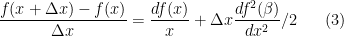
This formula provides an error term for an approximation of the derivative when is not zero. There are several important things to note about this formula. The first is that the Taylor series cannot be used if the function that is being approximated does not have at least two derivatives, i.e., it cannot be discontinuous.The second is that in numerical analyis it is the power of the coefficient
  in the error term that is important. In this case because the power is 1, the accuracy of the method is called first order.
 . In the example above only two points were used, i.e.,
  and
and  . A three point discrete approximation to a derivative is
Higher order accurate methods have higher order powers of
Expanding both terms in the numerator in Taylors series with remainder , subtracting the two series and then dividing by produces

Because of the power of 2 in the remainder term, this is called a second order method and assuming the derivatives in both examples are of similar size, this method will produce a more accurate approximation as the mesh size decreases. However, the second method requires that the function be even smoother, i.e., have more derivatives.
The highest order numerical methods are called spectral methods and require that all derivatives of the function exist. Because Richardson’s equation in a model based on the hydrostatic equations causes discontinuities in the numerical solution, even though a spectral method is used, spectral accuracy is not achieved. The discontinuities require large dissipation to prevent the model from blowing up and this destroys the numerical accuracy (Browning, Hack, and Swarztrauber 1989).
Currently modelers are switching to different numerical methods (less accurate than spectral methods but more efficient on parallel computers) that numerically conserve certain quantities. Unfortunately this only hides the dissipation in the numerical method and is called implicit dissipation (as opposed to the curent explicit dissipation).
Gerald,
I don’t see the point here. Your criticism applies equally to CFD. And yes, both do tend to err on the side of being overly dissipative. But does that lead to error in climate predictions? All it really means is more boring weather.
Nick,
You have not done a correct analysis on the difference between two solutions, one with the control forcing and the other with a perturbed (GHG) forcing. See my correct analysis on Climate Audit.
And yes if the dissipation is like molasses, then the continuum error is so large as to invalidate the model. The sensitivity of molasses to perturbations is quite different than that of air..
This post is entirely misleading. For the correct estimate see my latest posts on Climate Audit (I cannot post the analysis here because latex is not working here according to Ric). That estimate clearly shows that a linear growth in time as in Pat Frank’s manuscript is to be expected.
Jerry
\title{Analysis of Perturbed Climate Model Forcing Growth Rate}
\author{G L Browning}
\maketitle
Nick Stokes (on WUWT) has attacked Pat Frank’s article for using a linear growth in time of the change in temperature due to increased Green House Gas (GHG) forcing in the ensemble GCM runs. Here we use Stokes’ method of analysis and show that a linear increase in time is exactly what is to be expected.
1. Analysis
The original time dependent pde (climate model) for the (atmospheric) solution y(t) with normal forcing f(t) can be represented as
where y and f can be scalars or vectors and A correspondingly a scalar or matrix. Now supose we instead solve the equation

where is the Green House Gas (GHG) perturbation of f. Then the equation for the difference (growth due to GHG)
  is
is
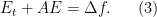
Multipy both sides by
Integrate both sides from 0 to t
Assume the initial states are the same, i.e., is 0. Then multiplying by
  yields
Taking norms of both sides the estimate for the growth of the perturbation is

where we have assumed the norm of as in the hyperbolic or diffusion case. Note that the difference is a linear growth rate in time of the climate model with extra CO2 just as indicated by Pat Frank.
Jerry
“That estimate clearly shows that a linear growth in time as in Pat Frank’s manuscript is to be expected.”
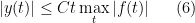
Well, firstly Pat’s growth is not linear, but as sqrt(t). But secondly, your analysis is just wrong. You say that
exp(-A*t) ∫ exp(A*u) f(u) du integration 0:t
has linear growth, proportional to max(|f|). Just wrong. Suppose f(u)=1. Then the integral is
exp(-A*t) (exp(A*t)-1)/A = (1-exp(-A*t))/A (6)
which does not grow as t (7), but is bounded above by 1/A.
In fact, the expression is just an exponential smooth of f(u), minus a bit of tail in the convolver.
Good try Nick. But f is not equal to 1 but to a vector of perturbations. And your formula does not work if A is singular as it is when there is no wind or in your example when you used the scalar A =0. And what does 1/A mean – is it suppose ot be the inverse? The estimate is the standard one for the integral of the solution operator times the forcing.
Now let me provide an additional lesson. Suppose the real equation is
but the model is solving
where $\epsilon_{l} >> \epsilon_{s} $
Subtracting equations as before the difference satisfies the equation
to a very good approximation.
This is a continuum error and one is essentially solving an equation for molasses and not
air.
You need to read Browning and Kreiss (Math Comp) to understand that using the wrong
type or amount of dissipation produces the wrong answer.
Jerry
All,
Note that Stokes’ scalar f = 1 is not time dependent as is the vector of time dependent perturbations. Nick chose not to mention that fact or to use a scalar function that is a function of time so he could mislead the reader. In fact if the scalar A is 0 (singular case),
the growth is proportional to t. The point of my Analysis is to show that Stokes’ analysis stated that the forcing drops out and that is also misleading to say the least.
In the case of excessively large dissipation in a model, I will rewrite the z equation as
Then the difference is
to a very good approximation. Now one can see that the difference equation E has a large added forcing term that does not disappear, i.e., a continuum error that means that one is not solving the correct equation.
Jerry
Jerry,
“Nick chose not to mention that fact or to use a scalar function that is a function of time so he could mislead the reader. “
I really have trouble believing that you were once a mathematician. If your formula fails when f=1, that is a counter-example. It is wrong. And you can’t save it by waving hands and saying – what if things were more complicated in some way? If you want to establish something there, you have to make the appropriate provisions and prove it.
Variable f doesn’t help – the upper bound is just max(||f||)/A
In fact my analysis covered three cases, case 1 (A=0) and case 3 (A>0 and A<0). As I said, with A0, it is bounded above as I showed. Indeed, as I also said, it is just the exponential smooth of f, minus a diminishing tail.
Matrix A won’t save your analysis either. The standard thing is to decompose:
AP=PΛ where Λ is the diagonal matrix of eigenvalues
Then set E=PG
PG’ + APG = PG’ + PΛG = f
or G’ + ΛG = P⁻¹f
That separates it into a set of 1-variable equations, which you can analyse in the same way.
Well Nick,
I will let my mathematics speak for themselves. I notice that you stated in reference to my Tutorial on Numerical Approximation:
“I don’t see the point here. Your criticism applies equally to CFD. And yes, both do tend to err on the side of being overly dissipative. But does that lead to error in climate predictions? All it really means is more boring weather.”
Yes, the criticism applies to any CFD models that mimic a discontinous continuum solution, i.e., then the numerics are not accurate.
At least you admitted that the CFD models tend to be ” overly dissipative”. But not what that does to the continuum solution with the real dissipation. My analysis shows that excessive (unrealistic) dissipation causes the model to converge to the wrong
equation. I guess you are saying there is no difference between the behavior of molasses and air. This is no surprise to me from someone that made a living using numerical models with excessive dissipation. And as I have said before you need to keep up with the literature. I mentioned two references that you have clearly not read or you would not continue to poo poo this common fudging technique in CFD and climate models.
Next you said
“I really have trouble believing that you were once a mathematician. If your formula fails when f=1, that is a counter-example. It is wrong. And you can’t save it by waving hands and saying – what if things were more complicated in some way? If you want to establish something there, you have to make the appropriate provisions and prove it.”
Is is not a counter example because the symbol A for a symmetric hyperbolic PDE can be singular and then you cannot divide by A (or more correctly multipliy by $ latex A^{-1}$. All cases of A must be taken into account for a theory to be robust. Note that the only thing I assumed about the solution operator $\exp ( A t)$ is that it is bounded. I assumed nothing about the inverse of A. The solution operator is bounded for all symmetric hyperbolic equations even if A is singular. Thus your use of the inverse is not a robust theory.
If my analysis is wrong, why not try a nonconstant function of t so you cannot divide by A? I thought so.
As far as your use of eigenvalue , eigenvector decomposition I am fully aware of that math.
For a symmetric hyperbolic system A leads to eignevalues that can be imaginary or 0
(so the solution operator is automatically bounded).
In the latter case A is singular so any robust theory must take that into account, i.e. you cannot assume that the inverse exists. Also note that f is a function of t, not a constant. You continue to avoid that issue because for an arbitrary nonconstant function of t,
the integral in general cannot be solved, but can be estimated as I have done.
It appears you just don’t want to accept the linear growth in time estimate. Good luck with that.
Jerry
“All cases of A must be taken into account for a theory to be robust. “
It is your theory that perturbations increase linearly with t. And it fails for the very basic case when A=1, f=1. And indeed for any positive A and any bounded f.
For matrix A, the problem partitions. And then, as indicated in my posts, there are three possibilities for the various eigenvalues and their spaces
1. Re(λ)>0 – perturbation changes with exponential smooth of driver, bounded if driver is bounded
2. Re(λ)=0 – perturbation changes as integral of driver
3. Re(λ)<0 – perturbation grows exponentially
Ok Nick,
Let us make clear what solution you are suggestiing in contrast to the one I am using. Green House Gases (GHG) in the atmosphere are increasing. So the climate modelers are injecting increasingly larger GHG (CO2) into the climate models over a period of time, i.e. the amount of CO2 in the model is changing. The forcing in the models depends on the amount of CO2 so the forcing in the models also is changing over time. You are assuming the additional forcing is constant in time which is clearly not the case. I on the other hand am allowing the forcing to change in time as is the case in reality. All you have to do to disprove my estimate is to make the physically correct assumption that the
increase in forcing is a function of time. Then your example will not work because the change in forcing is no longer constant. Quit making physically incorrect assumptions
and stating my correct one is wrong.
Also in my estimate of E, assuming the solution operator is bounded by a constant instead of unity leads to fact that by changing that constant by changing the amount of dissipation (or other tuning parameters) allows the modelers to change the amount of growth as they wish, even though it might not be physically realistic.
I also see that you must agree now with my Tutorial on the misuse of numerical approximations in models that mimic discontinuities in the continuum solution or
otherwise you would have made some assinine counter to that fact without proof.
And you have yet to counter with proof that using excessive dissipation alters the
solution of the pde with the correct amount of dissipation. This has been
shown with mathematical estimates for the full nonlinear compressible Navier -Stokes equations (the equations used in turbulence modeling) and demonstrated with convergent numerical solutions (Henshaw, Kreiss and Reyna). You need to keep up with the literature.
Jerry
“All you have to do to disprove my estimate is to make the physically correct assumption that the increase in forcing is a function of time.”
I dealt with that case:
“Variable f doesn’t help – the upper bound is just max(||f||)/A”
It makes no difference at all.
exp(-A*t) ∫ exp(A*u) f(u) du < exp(-A*t) ∫ exp(A*u) Max(f(u)) du
= Max(f(u))exp(-A*t) ∫ exp(A*u) du < Max(f(u))/A
and to complete the bounds:
-exp(-A*t) ∫ exp(A*u) f(u) du < Max(-f(u))/A
““Variable f doesn’t help – the upper bound is just max(||f||)/A””
How do you know the maximum of “f” if it is a function of time? What generates the upper bound in that case?
“How do you know the maximum”
It is here the maximum in the range. But it could be the overall maximum.
What if f itself increases without limit? Well, then of course perturbations could have similar behaviour.
Remember, Gerald has a specific proof claimed here. Perturbations increase linearly. You can’t keep saying, well it didn’t work here, but it might if we make it a bit more complicated. Maths doesn’t work like that. If a proof has counterexamples, it is wrong. Worthless. It failed. You have to fix it.
“It is here the maximum in the range. But it could be the overall maximum.
What if f itself increases without limit? Well, then of course perturbations could have similar behaviour.”
You *still* didn’t answer how you know the maximum so you can use it as a bound. What is the range. How is it determined? Is it purely subjective?
What if f *does* increase without limit? Isn’t that what an ever growing CO2 level would cause? At least according to the models that is what would happen.
If there *is* a limit then why don’t the models show that in the temperature increases over the next 100 years?
OK Nick,
It is getting easier and easier to rebut your nonsense
Consider your favorite scalar equation
with a a nonzero constant and f an arbitrary function of time as physically correct (not a constant as physically inappropriate as made clear above).
As before multiply by
$ latex ( \exp (at) y )_{t} = \exp (at) f(t)$
Integrate fron 0 to t
$ latex \exp (at) y (t) = \exp (0) y (0) + \int_{0}^{t)} \exp (a \tilde{t} ) f( \tilde{t} d \tilde{t}$
assuming the model with normal forcing and the model with added GHG forcing start from the same initial conditions
This becomes
$ latex y (t) = \int_{0}^{t)} \exp (a \tilde{t}-at) f( \tilde{t} d \tilde{t}$
Now for a positive, 0 or negative the exponential is bounded by a constant C for t finite.
Taking absolute values or both sides
and the estimate is exactly as in the full system, i.e., a bounded linear growth in time.
I have heard that when you are wrong you either obfuscate or bend the truth. I now fully believe that based on your misleading responses to my comments.
I am also waiting for your admission that discontinuous forcing causes the numerical solutuon of a model to mimic a discontinuous continuum solution invalidating the numerical analysis accuracy requirements of differentiability.
And I am also wating for your admission that using excessively large dissipation means that you are not solving the correct system of equations.
Jerry
Gerald,
“and the estimate is exactly as in the full system”
Well, it’s just a very bad estimate, and ignores the behaviour of the exponential. It’s actually a correct inequality. But it’s also true that E is bounded as I said. So it is quite misleading to say that E increases linearly with t. I have given several basic examples where that just isn’t true.
It is true also that E ≤ C exp(t²) for some C. That doesn’t mean that C increases as exp(t²).
That doesn’t mean that E increases as C*exp(t²).
“You *still* didn’t answer how you know the maximum so you can use it as a bound. “
Δf() is a prescribed function. If you prescribe it, you know if it has a maximum, and what it is.
But the whole discussion has been muddled by Gerald – I’m just pointing to the errors in his maths. In fact Pat Frank was talking about how uncertainty propagates in a GCM from uncertainty in cloud cover. He says it grows fast. Gerald has switched to a perturbation in temperature due to GHGs. Not uncertainty in GHGs, but just GHGs. And he claims they grow indefinitely.
Well, they might. It’s not usually a proposition promoted at WUWT. In fact, if GHGs keep growing indefinitely, temperatures will. This is totally unrelated to what Pat Frank is writing about.
OK Nick,
It is getting easier and easier to rebut your nonsense
Let us onsider your favorite scalar equation
title{Estimate of Growth for a Scalar Equation with Time Dependent Forcing}
\author{GL Browning}
\maketitle
Nick Stokes has claimed that the estimate for a scalar version of my difference equation E is different than the matrix version. Here we show that is not the case for all finite values of Re(a) and that by tweaking the amount of dissipation in the case , the linear growth rate can be changed arbitrarily.
1. Analysis
Consider the equation
with a being a constant and f an arbitrary function of time as physically correct (not a constant as physically inappropriate as made clear above). As before multiply by :
:

Integrating fron 0 to t

Assuming the model with normal forcing and the model with added GHG forcing start from the same initial conditions this becomes

Taking absolute values or both sides

Note that the quantity so changes the sign of a or is 0. Thus for Re(a) positive (dissipative) case, 0, or negative (growth case), the exponential is bounded by a constant C for t finite. So
from elementary calculus This is the same estimate as before, a bounded linear growth in time. Note that messing with the dissipation , C can be made to be whatever one wants.
I am waiting for your admission that discontinuous forcing causes the numerical solution of a model to mimic a discontinuous continuum solution invalidating the numerical analysis accuracy requirements of differentiability.
And I am also waiting for your admission that using excessively large dissipation means that you are not solving the correct system of equations.
All,
That didn’t come out very well as there is no preview. I will try again because this is important.
Some of you might not be familiar with complex variables.
I will add a bit of info that hopefully helps.
The derivative of an exponential with a real or complex exponent is the same so nothing changes in that part of the proof, i.e., the same formula holds whether a is a real or complex number. However, the absolute value of an exponential
with a complex number is just the absolute value of the exponent of the real part.
That is because the exponential of an imaginary exponent like $ latex \exp (i Im (a)t)$
is defined as $ latex cos( Im(a) t) + i sin ( Im(a) t)$ whose absolute value is 1.
Thus
$ latex | \exp ( ( Re(a) + i Im(a) ) t) | = | \exp ( Re(a) ) \exp ( i Im(a) )| = | \exp ( Re(a) ) | | | \exp ( i Im(a) )| = \exp ( Re(a) )$
Jerry
All,
I gave up trying to do this inside a comment and went outside where I could test everything.
All,
That didn’t come out very well as there is no preview. I will try again because this is important.
Some of you might not be familiar with complex variables. I will add a bit of info that hopefully helps.
The derivative of an exponential with a real or complex exponent is the same so nothing changes in that part of the proof, i.e., the same formula holds whether a is a real or complex number. However, the absolute value of an exponential with a complex number is just the absolute value of the exponent of the real part. That is because the exponential of an imaginary exponent like is defined as
whose absolute value is 1 because

Thus

Jerry
All,
Now let us discuss the case of exponentially growing in time solutions.
In the theory of partial differential equations there are only two classes of equations:
well posed systems and ill posed systems. In the latter case there is no hope to compute a numerical solution because the continuum solution grows exponentially unbounded in an infinitesmal amount of time. It is surprising how many times one comes across such equations in fluid dynamicals because seemingly reasonable physical assumptions lead to mathematical problems of this type.
The class of well posed problems are computable because the exponential growth rate (if any) is bounded for a finite time. As is well known in numerical analysis, if there are exponentially growing solutions of this type, they can only be numerically computed for a short period of time because the error also grows exponentialy in time. So we must assume that climate models that run for multiple decades either do not have any exponentially growing components or they have been suppressed by artificial excessively large dissipation. So assuming the climate models only have dissipattive
types of components, we have seen that the linear growth rate of added CO2 can be controlled to be what a climate modeler wants by changing the amount of dissipation.
I find that Pat Frank’s manuscript on the linear growth rate of the perturbations of temperature with added CO2 in the ensemble climate model runs as emminetlly reasonable.
Jerry
Nick, “Well, firstly Pat’s growth is not linear, but as sqrt(t)”
Jerry Browning is talking about the growth in projected air temperature, not growth in uncertainty.
The growth in uncertainty grows as rss(±t_i), not as sqrt(t).
That’s two mistakes in one sentence. But at least they’re separated by a comma.
“Jerry Browning is talking about the growth in projected air temperature”
His result, eq 7, says
“the estimate for the growth of the perturbation is…”
Nick,
If you look at the system, it is the growth due to the change (perturbation) in the forcing by adding GHG’s to the control forcing f (no GHC_). Don’t try to play gmes. The math is very clear as to what I was estimating.
Jerry
I
Gerald
“The math is very clear”
So where is a cause due to GHG entered into the math? How would the math be different if the cause were asteroids? or butterflies?
Nick,
You are clearly getting desperate. The magnitude of the change in forcing would change if the perturbation were from a butterfly or asteroid. Thus both are taken into account.
I await your use of the correct physical assumption that the change in forcing is a function of time.
Jerry
” The magnitude of the change in forcing would change if the perturbation were from a butterfly or asteroid. “
Your proof uses algebra, not arithmetic.
“Your proof uses algebra, not arithmetic.”
So what? The result is the same.
Also, I should have noted, in response to Nick’s Pat’s growth is not linear, but as sqrt(t)”, that growth in T goes as [(F_0+∆F_i)/F_0], which is as linear as linear ever gets.
“growth in T goes as [(F_0+∆F_i)/F_0], which is as linear as linear ever gets”
Well, in Eq 1 it was (F_0+Σ∆F_i)/F_0. But yes, by Eq 5.1 it has become (F_0+∆F_i)/F_0. None of this has anything to do with whether it grows linearly with time.
Ya lost me at “what you believe to be the correct number.”
You can be agnostic about that if you like. I’m showing how a discrepancy between to possible initial states is propagated in time by a differential equation. It could be a difference between what you think is right and its error, or just a measure of an error distribution. The key thing is what the calculation does to the discrepancy. Does it grow or shrink?
What would cause someone to BELIEVE a number to be correct, rather than to know with confidence that the number IS correct?
An unconfirmed BELIEF would seem to be a theoretical foundation of the model, and this belief itself could be subject to uncertainty — a theory error? … with accompanying uncertainty above and beyond the uncertainty of the performance of the calculation that incorporates this uncertain theoretical foundation?
This discussion is so far beyond me that I have to fumble with it in general terms. Nick’s presentation seems to be further effort to sink Pat Frank’s assessment, and so I’m caught between two competing experts light years of understanding ahead of me.
I still get the feeling that Pat is talking about something that is captured by Nick’s use of the word, “belief”, and so I’m not ready to let Pat’s ship sink yet.
‘and so I’m not ready to let Pat’s ship sink yet.”
pats boat sunk when he forgot that Watts are already a rate
One mistake renders an entire paper useless.
Unless you are a climate scientist.
Clarify. Thanks.
Steve is just parroting Nick Stokes’ mistake, Robert.
He actually doesn’t know what he’s talking about and so cannot clarify.
“Discrepancy” is not uncertainty.
“Discrepancy” is not uncertainty.
+1
Surely the correct number is what actually happens in the system being modelled using GCMs. Not much use if you’re trying to make predictions for chaotic systems.
Nick, could you explain how negative feedback affects propagating error, please?
Well, negative feedback is a global descriptor, rather than an active participant in the grid-level solution of GCMs. But in other systems it would act somewhat like like special case 3 above, with negative c, leading to decreasing error. And in electronic amplifiers, that is just what it is used for.
So you agree with the previous paper Monckton? That used an electrical feedback circuit to show GCMs were wrong
“That used an electrical feedback circuit to show GCMs were wrong”
Well, he never said how, and was pretty cagey about what the circuit actually did. But no, you can’t show GCM’s are wrong with a feedback circuit. All you can show is that the circuit is working according to specifications.
Well you can’t use ICE knowledge and design to defend climate models, either, but you tried.
Same goes for wind-tunnel tests.
Negative feedback is *NOT* to reduce error. In fact, in an op amp the negative feedback *always* introduces an error voltage between the input and the output. It is that error that provides something for the op amp to actually amplify. The difference may be small but it is always there.
This is basically true for any physical dynamic system, whether it is the temperature control mechanism in the body or the blood sugar level control system.
“For the case of continuous errors, the earlier ones have grown a lot by the time the later ones get started, and really are the only ones that count. So it loses the character of random walk, because of the skewed weighting“
So the GCM’s are then worse at error propagation than we thought. The similarity in TCF error hindcast residuals between GISS-er and GISS-eh (Frank’s Figure 4. and discussion therein) tells us that the errors are systematic, not random. And those TCF systematic errors start at t=0 in the GCM simulations.
“So the GCM’s are then worse at error propagation than we thought.”
Well, not worse than was thought. Remember the IPCC phrase that people like to quote:
“In climate research and modelling, we should recognise that we are dealing with a coupled non-linear chaotic system, and therefore that the long-term prediction of future climate states is not possible. The most we can expect to achieve is the prediction of the probability distribution of the system’s future possible states by the generation of ensembles of model solutions. This reduces climate change to the discernment of significant differences in the statistics of such ensembles”
It comes back to the chaos question; there are things you can’t resolve, but did you really want to? If a solution after a period of time has become disconnected from its initial values, it has also become disconnected from errors in those values. What it can’t disconnect from are the requirements of conservation of momentum, mass and energy, which still limit and determine its evolution. This comes back to Roy Spencer’s point, that GCM’s can’t get too far out of kilter because TOA imbalance would bring them back. Actually there are many restoring mechanisms; TOA balance is a prominent one.
On your specific point – yes, DEs will generally have regions where they expand error, but also regions of contraction. In terms of eigenvalues and corresponding exponential behaviour, the vast majority correspond to exponential decay, corresponding to dissipative effects like viscosity. For example, if you perturb a flow locally while preserving angular momentum, you’ll probably create two eddies with contrary rotation. Viscosity will diffuse momentum between them (and others) with cancellation in quite a short time.
So the values at any point in time are going to be bounded by the conservation laws? Temperatures may go up, but regardless of any error propagation, they won’t reach the melting point of lead.
“This comes back to Roy Spencer’s point, that GCM’s can’t get too far out of kilter because TOA imbalance would bring them back. Actually there are many restoring mechanisms; TOA balance is a prominent one.”
Each additional W/m2 leads to 0.5 to 1°C of warming. About the same effect as a third of a percent change of albedo. Seriously, how far out of kilter does it have to get to come up with 8 °C climate sensitivity?
Robert B
There is no way the sensitivity can be that high. Have a look at the insolation difference between summer and winter in the northern and southern hemispheres. The two are isolated enough for a difference of dozens of Watts/m^2 to produce a temperature difference. If the sensitivity was 0.5 to 1.0 C per Watt, the summers in the South would be dozens of degrees warmer than summers in the North. They are not.
Crispin,
That is a good point.
It applies not just to a temperature comparison of the northern and southern hemispheres, but also to what could happen within each hemisphere, i.e., no drastic excursions could happen because other factors would offset them, i.e., the weather comes and goes, then settles to some average climate state.
Any climate changes due to mankind’s efforts are so puny they could affect the hemisphere climate only very slowly, if at all.
Not my estimate.
My point was that 298^4/290^4 is about 1.1 so 10% more insolation for a real blackbody or dropping albedo by a third. According to the estimate, at most an extra 16W/m2 needed for 8 degree increase which is the high end of modelling. That is about 1/6 drop in albedo. The 8°C is out of kilter and needed to be chucked in the bin, and 4 is dodgy.
So why do the GCM models only show warming, when cooling happens? Where is that bias forced? When terms fudged, parameterized, or ignored is the error distribution reset?
The IPCC quote is very much to the topic.
“This reduces climate change to the discernment of significant differences in the statistics of such ensembles”.
The ongoing problem is that there is only going to be one result over future time. The need is for one model that produces the future climate down to the acre.
Having 40-50 models that can produce projection graphs 100 years into the future is useless if none of the graphs can be shown to be predictive. Planning for the future when the prediction is that at any given point in time the temperature will be within a range that grows exponentially over 80 years from +/-.1deg to +/- 3deg is not useful or effective.
What Mr. Frank was trying to demonstrate was that the models have such a wide, exponentially growing error range, as shown in the many versions of AR5 graphs, that the results aren’t predictive in any way, shape, or form after just a few years.
“If a solution after a period of time has become disconnected from its initial values, it has also become disconnected from errors in those values. ”
The problem isn’t the error in the initial values, the problem is the uncertainty of the outputs based on those inputs. The uncertainty does *not* become disconnected.
If your statement here were true then it would mean that the values of the initial value could be *anything* and you would still get the same output. The very situation that causes most critics to have no faith in the climate models.
Tim Gorman
Yes, it would seem that Stokes is arguing that GCMs violate the GIGO principle.
The GCM’s are unstable. They have code that purposely flattens out the temperature projections because they too often blew up. Modelers have admitted this. Also Nick you said :
“It is just a discrepancy between a number that arises in the calculation, and what you believe is the true number.” THAT IS WRONG. What you believe is not important. What is important is the true number that is backed up by observations that you obtain by running real world experiments.
“The most we can expect to achieve is the prediction of the probability distribution of the system’s future possible states by the generation of ensembles of model solutions. ” That statement by the IPCC is so mathematically wrong and illogical that it defies belief. You CANNOT IMPROVE A PROBABILITY DISTRIBUTION BY RUNNING MORE SIMULATIONS OR USING MORE MODELS THAT HAVE THE SAME SYSTEMATIC ERROR.
As such the title to Nick’s essay should read, “How random error propagation works with differential equations (and GCMs)”.
And let’s be clear here, Lorenz’s uncertainties that Nick spent a great effort explaining with nice diagrams, were due to random error sets in initialization conditions.
The visual message of Frank’s Figure 4 (of the general similarity of the TCF errors) should be the big clue of what the modellers are doing to get their ECS so wrong from observation.
The TOA energy balance boiling pot argument… schamargument,
the random error propagation… schamargation…
You don’t get systematic errors that looks so similar (Fig 4 again) without the “common” need for a tropospheric positive feedback in the atmosphere that obviously isn’t there.
What a tangled web we weave, when first we endeavor to deceive.
(not you Nick, but the modellers needing (expecting?) a high ECS.)
“As such the title to Nick’s essay should read”
Actually, no. I’m showing what happens to a difference between initial states, however caused.
” Lorenz’s uncertainties … were due to random error sets in initialization condition”
Again, it doesn’t matter what kind of errors you have in the initial sets. Two neighboring paths end up a long way apart quite quickly. I don’t think Lorenz invoked any kind of randomness.
Nick Stokes: Actually, no. I’m showing what happens to a difference between initial states, however caused.
That much is true. That is not what Pat Frank was doing. He was deriving an approximation to the uncertainty in the model output that followed from uncertainty in one of the model parameters. The uncertainty in the model parameter estimate was due in part to random variation in the measurement errors and other random influences on the phenomenon measured; the uncertainty in the propagation was modeled as random variation consequent on random variation in the measurements and the parameter estimate. That variation was summarized as a confidence interval.
You have still, as far as I have read, not addressed the difference between propagating an error and propagating an interval of uncertainty.
BINGO!
IOW, still trying to change the subject in a manner that supposedly undermines Pat Frank’s analysis and conclusions.
“I am not sure how many ways to say this, but the case analysed by Pat Frank is the case where A is not known exactly, but is known approximately”
He analysed the propagation of error in GCMs. In GCMs A is known; it is the linearisation of what the code implements. And propagation of error in the code is simply a function of what the code does. Uncertainty about parameters in the GCM is treated as an error propagated within the GCM. To do this you absolutely need to take account of what the DE solution process is doing.
As to
“the difference between propagating an error and propagating an interval of uncertainty”
there has been some obscurantism about uncertainty; it is basically a distribution function of errors. Over what range of outputs might the solution process take you if this input, or this parameter, varied over such a range. The distribution is established by sampling. A one pair sample might be thought small, except that differential equations, being integrated, generally give smooth dependence – a near linear stretching of the solution space. So the distribution scales with the separation of paths.
Nick Stokes: In GCMs A is known;
That is clearly false. Not a single parameter is known exactly.
That is one of the ways that you are missing Pat Frank’s main point: you are regarding as known a parameter that he regards as approximately known at best, within a probability range.
There has been some obscurantism about uncertainty; it is basically a distribution function of errors. Over what range of outputs might the solution process take you if this input, or this parameter, varied over such a range. The distribution is established by sampling. A one pair sample might be thought small, except that differential equations, being integrated, generally give smooth dependence – a near linear stretching of the solution space. So the distribution scales with the separation of paths.
You start well, then disintegrate. What “scales” if you start with the notion of a distribution of possible errors (uncertainty) in a parameter is the variance in the uncertainty of the outcome. That is what Pat Frank computed and you do not.
I showed how in my comment on your meter stick of uncertain length. If you are uncertain of its length then your uncertainty in the resultant measure grows with the distance measured. I addressed two cases: the easy case where the true value is known exactly within fixed bounds; the harder case where the uncertainty is represented by a confidence interval. You wrote as though the error could become known, and adjusted for — that would be bias correction, not an uncertainty propagation.
Not everyone accepts, or is prepared to accept, that the unknowableness of the parameter estimate implies the unknowableness of the resultant model calculation; or that the “unkowableness” can be reasonably well quantified as the distribution of the probable errors, summarised by a confidence interval. That “reasonable quantification of the uncertainty” is the point that I think you miss again and again. Part of it you get: There has been some obscurantism about uncertainty; it is basically a distribution function of errors. But you seem only to concern yourself with the errors in the starting values of the iteration, not the distribution of the errors of the parameter values. Thus a lot of what you have written, when not actually false (a few times, as I have claimed), has been irrelevant to Pat Frank’s calculation.
“But you seem only to concern yourself with the errors in the starting values of the iteration, not the distribution of the errors of the parameter values.”
Pat made no useful distinction either – he just added a bunch of variances, improperly accumulated. But the point is that wherever the error enters, it propagates by being carried along with the flow of the DE solutions, and you can’t usefully say anything about it without looking at how those solutions behave.
On the obsrurantism, the fact is that quantified uncertainty is just a measure of how much your result might be different if different but legitimate choices had been made along the way. And the only way you can really quantify that is by observing the effect of different choices (errors), or analysing the evolution of hypothetical errors.
“Nick Stokes: In GCMs A is known;
That is clearly false. “
No, it is clearly true. A GCM is a piece of code that provides a defined result. The components are known.
It is true that you might think a parameter could in reality have different values. That would lead to a perturbation of A, which could be treated as an error within the known GCM. But the point is that the error would be propagated by the performance of the known GCM, with its A. And that is what needs to be evaluated. You can’t just ignore what the GCM is doing to numbers if you want to estimate its error propagation.
Nick Stokes: No, it is clearly true. A GCM is a piece of code that provides a defined result. The components are known.
It is true that you might think a parameter could in reality have different values. That would lead to a perturbation of A, which could be treated as an error within the known GCM. But the point is that the error would be propagated by the performance of the known GCM, with its A. And that is what needs to be evaluated. You can’t just ignore what the GCM is doing to numbers if you want to estimate its error propagation.
That is an interesting argument: the parameter is known, what isn’t known is what it ought to be.
We agree that bootstrapping from the error distributions of the parameter estimates is the best approach for the future: running the program again and again with different choices for A (well, you don’t use the word bootstrapping, but you come close to describing it.) Til then, we have Pat Frank’s article, which is the best effort to date to quantify the effects in a GCM of the uncertainty in a parameter estimate. I eagerly await the publication of improved versions. Like Steven Mosher’s experiences with people trying to improve on BEST, I expect “improvements” on Pat Frank’s procedure to produce highly compatible results.
Your essay focuses on propagating the uncertainty in the initial values of the DE solution. You have omitted entirely the problem of propagating the uncertainty in the parameter values. You agree, I hope, that propagating the uncertainty of the parameter values is a worthy and potentially large problem to address. You have not said so explicitly, nor how a computable approximation might be arrived at in a reasonable lenght of time with today’s computing power.
“You have omitted entirely the problem of propagating the uncertainty in the parameter values.”
No, I haven’t. I talked quite a lot about the effect of sequential errors (extended here), which in Pat Frank’s simple equation leads to random walk. Uncertainty in parameter values would enter that way. If the parameter p is just added in to the equation, that is how it would propagate. If it is multiplied by a component of the solution, then you can regard it as actually forming part of a new equation, or say that it adds a component Δp*y. To first order it is the same thing. To put it generally, to first order (which is how error propagation is theoretically analysed):
y0’+Δy’=(A+ΔA)*(y0+Δy)
is, to first order
y0’+Δy’=A*(y0+Δy)+ΔA*y0
which is an additive perturbation to the original equation.
Nick Stokes: Uncertainty in parameter values would enter that way.
So how exactly do you propagate the uncertainty in the values of the elements of A? You have alternated in consecutive posts between claiming that the elements of A are known (because they are written in the code), and claiming that the parameter values used in calculating the elements of A are uncertain.
Pat Frank’s procedure is not a random walk; it does not add a random variable from a distribution at each step, it shows that the variance of the uncertainty of the result of each step is the sum of the variances of the steps up to that point (the correlations of the deviations at the steps are handled in his equations 3 and 4.) How exactly have you arrived at the idea that his procedure generates a random walk? Conditional on the parameter selected at random from its distribution, the rest of the computation is deterministic (except for round-off error and such); the uncertainty in the value of the outcome depends entirely on the uncertainty in the value of the parameter, not on randomness in the computation of updates.
I think your idea that a parameter whose value is approximated with a range of uncertainty becomes “known” when it is written into the code is bizarre. If there are 1,000 values of the parameter inserted into the code via a loop over the uncertainty range (either over a fixed grid or sampled pseudo-randomly as in bootstrapping), you would treat the parameter value (the A matrix) as “known” to have 1,000 different values. That is (close to) the method you advocate for estimating the effect of uncertainty in the parameter on uncertainty in the model output.
“it does not add a random variable from a distribution at each step, it shows that the variance of the uncertainty of the result of each step is the sum of the variances of the steps up to that point”
No, it says that (Eq 6) the sd σ after n steps (not of the nth step) is the sum in quadrature of the uncertainties (sd’s) of the first n steps. How is that different from a random walk?
You keep coming back to Eq 3 and 4, even though you can’t say where any correlation information could come from. Those equations were taken from a textbook; there is no connection made with the calculation, which seems to rely entirely on Eq 5 and Eq 6. There isn’t information provided to do anything else.
“I think your idea that a parameter whose value is approximated with a range of uncertainty becomes “known” when it is written into the code is bizarre.”
No, it is literally true. There is an associated issue of whether you choose to regard it as a new equation, and solve accordingly, or regard it as a perturbing the solutions of of the original one. The first would be done in an ensemble; the second lends itself better to analysis. But they are the same to first order in perturbation size.
Nick,
“the sum in quadrature of the uncertainties”
I believe you are trying to say that the uncertainties cancel. Uncertainties don’t cancel like errors do. Uncertainties aren’t random in each step.
“I believe you are trying to say that the uncertainties cancel.”
I’m saying exactly what eq 6 does. It is there on the page.
Nick,
What eq 6 are you talking about? Dr Frank’s? The one where he writes:
“Equation 6 shows that projection uncertainty must increase with every simulation step, as is expected from the impact of a systematic error in the deployed theory.”
That shows nothing about uncertainties canceling.
Or are you talking about one of your equations? Specifically where you say “where f(t) is some kind of random variable.”?
The problem here is that uncertainty is not a random variable. You keep trying to say that it is so you can depend on the central limit theory to argue that it cancels out sooner or later. But uncertainty never cancels, it isn’t random. If a model gives the same output no matter what the input is then the model has an intrinsic problem, it can just be represented by a constant. If the input is uncertain then a proper model will give an uncertain output, again if it doesn’t then it just represents a constant. What use is a model that only outputs a constant?
“That shows nothing about uncertainties canceling.”
You made that up. I said nothing about uncertainties cancelling. I said they added in quadrature, which is exactly what Eq 6 shows. He even spells it out:
“Thus, the uncertainty in a final projected air temperature is the root-sum-square of the uncertainties in the summed intermediate air temperatures.”
“You made that up. I said nothing about uncertainties cancelling. I said they added in quadrature, which is exactly what Eq 6 shows. He even spells it out:
“Thus, the uncertainty in a final projected air temperature is the root-sum-square of the uncertainties in the summed intermediate air temperatures.””
So you admit the uncertainties do not cancel, correct?
Nick, many thanks for this, and many thanks to WUWT for hosting it. This is what makes this site different.
As much as I dislike’s Nick’s stubbornness and refusal to admit when he’s wrong (a trait he has in common with Mann) he does occasionally provide useful insight.
In addition to models being reflections of their creators and tuning, there’s there’s the lack of knowing the climate sensitivity number for the last 40 years.
They should probably name a beer after climate modeling, called “Fat Tail”.
https://wattsupwiththat.com/2011/11/09/climate-sensitivity-lowering-the-ipcc-fat-tail/
Anthony Watts
September 16, 2019 at 7:53 pm
Well, I personally would like to thank Anthony for running such a great site that actually allows Nick and his colleagues to have an input. Otherwise we are talking to ourselves, and what’s the point of that?
I often don’t agree with what Nick posts but I always learn something from the comments that inevitably ensue. It’s such a fun way to learn and you never know just what tangent you are going to be thown off into.
The main thing I have learnt here is that the science is NOT settled!
The other great thing about WUWT is that (mostly) comments remain polite and civil. Everyone here appears to be an adult, unlike most other sites. So, thanks also to the moderators.
I’m with Alastair. I appreciate WUWT hosting someone like Nick, who we may disagree with, but is rational, polite and adds to the discourse. I often find that skeptical positions are improved and refined in the responses to the objections that Nick raises.
“Well, I personally would like to thank Anthony for running such a great site that actually allows Nick and his colleagues to have an input. Otherwise we are talking to ourselves, and what’s the point of that?”
I couldn’t agree more. We want to hear from all sides. We are not afraid of the truth.
Except for Griff, free the Griff! 😉
Yes, thanks to Anthony.
I’d like to add my thanks to WUWT for hosting it. I hope it adds to the discussion.
Nick Stokes Thanks for highlighting the consequences of modeling chaotic climate.
Now how can we quantify model uncertainty? Especially Type B vs Type A errors per BIPM’s international GUM standard?
Guide for the Expression of Uncertainty in Measurement (GUM).
See McKitrick & Christy 2018 who show the distribution and mean trends of 102 IPCC climate model runs. The chaotic ensemble of 102 IPCC models shows a wide distribution within the error bars. (Fig 3, 4)
However, the mean of the IPCC climate models are running some 285% of the independent radiosonde and satellite data since 1979, assuming a break in the data.
That appears to indicate that IPCC models have major Type B (systematic) errors. e.g., the assumed high input climate sensitivity causing the high global warming predictions for the anthropogenic signature (Fig 1) of the Tropical Tropospheric Temperatures. These were not identified by the IPCC until McKitrick & Christy tested the IPCC “anthropogenic signature” predictions from surface temperature tuned models, against independent Tropical Tropospheric Temperature (T3) data of radiosonde, satellite, and reanalyses.
McKitrick, R. and Christy, J., 2018. A Test of the Tropical 200‐to 300‐hPa Warming Rate in Climate Models. Earth and Space Science, 5(9), pp.529-536.
https://agupubs.onlinelibrary.wiley.com/doi/full/10.1029/2018EA000401
Evaluation of measurement data — Guide to the expression of uncertainty in measurement
Look forward to your comments.
So do I . . .
David,
“Now how can we quantify model uncertainty?”
Not easily. Apart from anything else, there are a huge number of output variables, with varying uncertainty. You have mentioned here tropical tropospheric temperature. I have shown above a couple of non-linear equations, where solution paths can stretch out to wide limits. That happens on a grand scale with CFD and GCMs. The practical way ahead is by use of ensembles. Ideally you’d have thousands of input/output combinations, which would clearly enable a Type A analysis in your terms. But it would be expensive, and doesn’t really tell you what you want. It is better to use ensembles to explore for weak spots (like T3), and hopefully, help with remedying.
Nick, thanks for the discussion. Rational dialogue beats the diatribe we are constantly subjected to in the climate debate.
It seems to me that we can argue ad nauseum about error propagation in models. But there is still one and only one test of models that is relevant. I’ll let Richard Feynman do the talking. The following is from a video at http://www.richardfeynman.com/.
Now I’m going to discuss how we would look for a new law. In general we look for a new law by the following process. First we guess it. [Laughter.] Then we… well don’t laugh, that’s really true. Then we compute the consequences of the guess to see what… if this is right… if this law that we guessed is right. We see what it would imply. And then we compare the computation results to nature, or we say compare to experiment or experience… compare it directly with observation to see if it… if it works. If it disagrees with experiment, it’s wrong. In that simple statement is the key to science. It doesn’t make a difference how beautiful your guess is, it doesn’t make a difference how smart you are, who made the guess, or what his name is [laughter], if it disagrees with experiment, it’s wrong [laughter]. That’s all there is to it.
I am not an expert on GCMs, but I often see graphs comparing GCM forecasts/projections/guesses with reality, and unless the creators of the graphs are intentionally distorting the results, the GCMs consistently over-estimate warming. It’s one thing to know how error propagates when we know the form of the equations (which is an implicit assumption in your discussion), but quite something else when we don’t.
It’s one thing to know how error propagates when we know the form of the equations (which is an implicit assumption in your discussion), but quite something else when we don’t.
repeated for effect.
“quite something else when we don’t”
With GCMs we do. They may not be perfect models of reality. But this article is discussing the error propagation of the equations we have and use.
With GCMs we do. They may not be perfect models of reality.
So we do….but we don’t. LOL.
We know the equations in the models, david. They may be numerical estimates for the solutions to differential equations, they may leave-out or treat certain processes in a bulk manner, etc, and be a poor representative for reality…but we know what the equations are.
We know the equations in the models, david.
Of course we do. That wasn’t Randy’s point.
Stokes
You said, “I have shown above a couple of non-linear equations, where solution paths can stretch out to wide limits.” This sounds very much like you are qualitatively supporting Frank’s claim, even if you disagree at the quantitative level.
You had also said above, “… yes, DEs will generally have regions where they expand error, but also regions of contraction.” Do the contractions only occur with negative feedback? This sounds like an intractable problem where you never really know whether the uncertainty is within acceptable bounds or not. How would you recommend dealing with this? I’m not comfortable with the ensemble approach because what little I know about it suggests that the results can vary even when the same inputs are used in repetitive runs. If the outputs vary (with or without changing input variables) do the uncertainty errors vary as well?
Clyde,
“This sounds very much like you are qualitatively supporting Frank’s claim”
Firstly I’m saying that no such claim makes sense without looking at the underlying DE, which he does not do. But second, in the discussion on chaos, I’m pointing out that in terms of climate model performance, it’s looking at the wrong thing. We know that GCMs lose the information in the initial conditions (as does CFD). So there actually isn’t any point in trying to analyse what happened to error in the ICs. What counts is how the model handles the flux balances that it makes along the way.
Nick, “If a solution after a period of time has become disconnected from its initial values, it has also become disconnected from errors in those values.”
That does not mean the solution is correct.
“DEs will generally have regions where they expand error, but also regions of contraction.”
The analytical issue is predictive uncertainty not error. Big mistake.
“This comes back to Roy Spencer’s point, that GCM’s can’t get too far out of kilter because TOA imbalance would bring them back.”
Roy Spencer’s argument turns upon his fatal misapprehension that a calibration error statistic is an energy flux.
Nick, “If a solution after a period of time has become disconnected from its initial values, it has also become disconnected from errors in those values.”
That does not mean the solution is correct.
—————————————–
If a solution becomes disconnected from its initial value then that means the initial values are meaningless. They could be anything. That’s just confirmation that the models are designed to produce a specific output regardless of inputs!
Spencer, learn some manners.
Greg
Whom are you presuming to lecture, me or Roy? I didn’t realize that well-mannered people lectured others. Or do you consider yourself above your own advice?
Spencer
” I didn’t realize that well-mannered people lectured others.”
No they usually don’t, Spencer.
I’m near to 70 years old, and would NEVER AND NEVER be of such subcutaneous arrogance to name a commenter like you do.
“Stokes”
By intentionally, repeatedly naming Dr Stokes that way, you show where you are…
Perfect.
Rgds
J.-P. Dehottay
Bindidon
It has already been established that I’m lacking manners. What is your beef? You and Greg referred to me by my surname! I reserve the familiarity of first names to those who I consider to be friends or at least not antagonistic to me. Not many people refer to Dr. Einstein by his formal title. It is, after all, a little redundant. If you or Stokes accomplish as much as Einstein, I’ll consider officially recognizing that you have a sheepskin. However, I consider it pretentious to insist that those who have completed the hoop jumping be addressed with an honorific title.
BTW, for what it is worth, I’m older than you by several years. How about showing a little respect for age?
Bindidon;
I’m reminded of a joke:
Dr. Smith is driving to his office and not paying close attention to things around him; he is busy checking his smartphone for his golfing appointment times. He is in a fatal accident and the next thing he is aware of is that he is at the end of a very long line outside of what is obviously the Pearly Gates. After getting his bearings, he walks up to the head of the line to speak with Saint Peter.
When he gets to Saint Peter he says, “Hello, I’m Doctor Smith and apparently I’ve just died. I’d like to get into Heaven.” Saint Peter looks down at him and says, “Yes, while you are earlier than expected, I know who you are. Please return to your position in line and I’ll process you when your turn comes.”
Dr. Smith blusters, “But, but, I’m a doctor. I have spent my entire career in the service of mankind healing the sick and living a good life. I have made generous contributions to various benevolent societies and my golf club. I’m not used to waiting. People wait for me!” Saint Peter replies, “Up here you are just like everyone else. Only the good people get this far, but I have some perfunctory tests to perform before I can allow you in. Now, end of the line!”
With head down and heavy heart, Dr. Smith trudges back to the end of the line, resigned to the fact that he will not get special treatment in heaven just because of his title. The line moves very slowly. It is even worse than the Department of Motor Vehicles! After a few years, a grizzled old man, stooped with age and carrying a little black bag with MD on the side, walks past the line, talks briefly with Saint Peter, and enters Heaven.
Dr. Smith is incensed! He runs back up to the font of the line and impertinently yells at Saint Peter, “Why are you making me stand in line while you let that other doctor just stroll right in?” Saint Peter adjusts his glasses so that he can look over the top of them, and sternly says, “You are mistaken! That was not a doctor. That was God. He only thinks he is a doctor.”
———
It isn’t just MDs that are afflicted with the problem of inflated self-importance. Even many lowly PhDs (and those who worship authority) suffer from a lack of perspective and think that somehow they should be accorded more respect because they have demonstrated the 1% inspiration and 99% perspiration that is required for an advanced degree. What they do with that degree is rarely taken into consideration. After all, they have achieved the penultimate accomplishment in life!
The spirit of the Title of Nobility Clause of the US Constitution is to discourage special privileges of citizens based on class or the seductive award of titles. That is, “One man, one vote.” People may receive respect from others for their accomplishments, but they shouldn’t expect that it is owed to them based on education alone. People have to earn my respect.
https://en.wikipedia.org/wiki/Title_of_Nobility_Clause
P.S. You said, “… would NEVER AND NEVER be of such subcutaneous arrogance to name a commenter like you do.” However, despite your protest, you demonstrated the falsity of your claim by addressing me the same way! I guess “never” means something different for you than it does me.
By all means reserve first name terms for friends, that does not prevent you from being polite to others. Calling someone by their surname when addressing them directly is obviously and intentionally being offensive, for no better reason than disagree about some aspect of climate.
I do that in addressing you above to reflect back your own offensive attitude. I tell you to learn some manners as one would correct in insolent child, since that is the level of maturity you are displaying.
Now learn some manners, and stop answering back !
Nick Stokes
What good are 1000s of runs to further quantify Type A uncertainty analysis – when ALL the models fail by 285% from Type B uncertainty when tested against independent climate data of Tropical Tropospheric Temperatures?
1) *** Why not fix this obvious Type B error first? ***
2) *** Are there other independent tests of climate sensitivity to confirm/disprove
this massive Type B error? ***
I am not a statistical expert ( but I have stayed at Best Western many times ).I am thinking type A is what Nick is doing. Basically evaluating the errors generated within the GCM itself. While type B is what Pat is doing, basically using external information to generate the uncertainties. In Pat’s case the external data itself is experimental, actual, real data.
The common shape of TCF error shown in Pat Frank’s Figure 4 is a damning piece of evidence of a common systematic bias programmed into many (most?) of the GCMs.
Computer models simply quantify a theory or hypothesis. Ultimately they are either able to predict what happens in the real climate or not. How their errors arise and propagate is important, but less so than their failure to predict real world results they are said to “model”
The various 100+ global climate models starting back in the late 1980’s have consistently missed the mark….The Earth has heated far less than they predicted. Continuous ad hoc adjustments in the data and recalibration of the models fails because the modellers refuse, as yet it seems, to create models strong on the natural negative feedbacks against temperature rise that our climate possesses. Also they do not seem to model for possible saturation effects producing diminishing forcing from CO2 as its concentration arises.
The current religion-like conviction that climate catastrophe is imminent is preventing these presumably intelligent scientists from doing unbiased work. They defend a belief rather than search for truth.
+1
+1
+1
“I am thinking type A is what Nick is doin”
Pretty much. Ensemble is really a poor man’s Monte Carlo, limited by compute power.
And limited by the fact that we are really only guessing at the biases in the wheel. It may be a perfectly balanced system with lots of randomness about observed results, or it could be worn and wobbly. We’re paying attention to hurricanes in my part of the world, and ‘ensembles get a lot of play in the press. There are some serious outliers early, and often late. The differences between the real storm and to forecasts may be trivial to those thousands of miles away, but they make a heck of a difference to those 20 miles from the eye wall.
It doesn’t give one confidence that the modeling is up to the task of predicting real world behavior or validating a theory when considering weather systems….that discussion of errors n the models can be valid and useful, but it is not a discussion about whether the models are predicting a climate causation theory that is or is not being validate by live data which is or is not being diddled with.
The prediction doesn’t tell us where a hurricane will go. The hurricane validates, or does not, the utility of the forecast model(s).
If you are a long way away from the storm the models are pretty good. But it seems like more often that not, I’ve put up the shutters when I don’t need to.
I think the model = real life equation need a lot of work on the climate side before I’ll take action, & iy would be sure be nice if we tracked ‘climate’ with the public accuracy and detail devoted to hurricanes.
Wind tunnels still exist because people cannot yet accept CFD as the the final say on aircraft design
It is almost impossible to model uncertainty in chaotic systems..
The analogy I like to use is a racing car crash. Perhaps some of you follow Formula 1 or Indy car or Nascar.
The difference of a few mm can result in a crash, or none.
Other issues of mm can decide whether or not the crash involves other cars and no one can predict at the start of the race that there will be a crash or where the pieces of car will end up. You would be a fool to try.
Predicting a global climate is somewhat akin to that.
All one can really do is for example say that if the cars are closely matched it increases the chance of a crash. Or if they are very disparate so they get lapped a lot, that also increases the chance. Maybe.
Nick is as bad as Brenchley at blinding with irrelevant BS, At making complicated things impenetrable.
At using one word to describe something different.
The fact is that GCMs are really not fit to forecast more than a few days ahead. That we don’t even have the right partial differential equations to integrate, have no idea of the starting values and have to fudge things so they work at all. We don’t even really understand the feedbacks inherent in the climate, and we have proved that we don’t.
All we can say is that long term there appears to be enough negative feedback to not freeze ALL of the oceans and not let the earth get much warmer than it already is, no matter how much historical CO2 it has had.
If people didn’t live in man made cities and suburbs they would never for an instant conceive of the ludicrous possibility that humans could control the climate.
Country slickers and city bumpkins these days.
…and if you can model certainties in a chaotic system that system is no longer chaotic.
Yes, absolutely; plus nothing of his article was cast into the standard language of the GUM, including probability distributions, or applying equation (10) of the GUM to calculate combined uncertainties from the measurement equation (1), Y = f(X1, X2, X3, … Xn).
It would also be quite interesting to see Monte Carlo methods applied to a GCM as per the GUM, varying all the adjustable parameters over their statistical ranges and distributions (GUM Supplement 1, “Propagation of distributions using a Monte Carlo method”, JCGM 101:2008).
A post elsewhere that highlights the problem Nick is trying to address
“how is it that we can reasonably accurate calculate GMST with only about 60 gauges? I know that ATTP has had at least one blog post in that regard. Now, I think that error improves as the (inverse) square root of the number of gauges. The average is twice as accurate for N = 3,600, not proportional to the square root of N but proportional to the inverse square root of N.”
–
GMST is such a fraught concept.
Problem one is the definition of the surface on a mixed changing atmospheric world (variable water vapour) plus a mixed solid/liquid “surface of variable height and depth on top of an uneven shape with long term variability in the spin and torque and inclination of the world plus the variation in distance from the heating element plus variation in the shade from the satellite at times and albedo variation from clouds and volcanic emissions and ice and dust storms and heating from volcanic eruptions and CO2 emmision and human CO2 emissions.
Phew.
–
We could get around this partly by measuring solar output, albedo change and earth output from space by satellites and just using a planetary emmision temperature as a substitute for GMST.
You could actually compute what the temperature should be at any location on earth purely by it’s elevation, time of year and orientatation in space to the sun without using a thermometer.
–
In a model world, barring inbuilt bias, one only ever needs one model thermometer. There can be no error. Using 3600 does not improve the accuracy.
In a model world allowing a standard deviation for error will lead to a possible Pat Frank scenario. The dice can randomly throw +4W/m-2 for ever. Having thrown one head is no guarantee that the next throw or the next billion throws will not be a head.
Using 3600 instead of 60 does not improve the accuracy at all. It improves the expectation of where the accuracy should be is all. While they look identical accuracy and expectation of accuracy are two completely different things. Your statement on probability is correct.
–
Finally this presupposes a model world and temperature and reasonable behaviour. Thermometers break,or degrade over time, people enter results wrongly,or make them up or take them at the wrong time of day or average them when missing ( historical). The accuracy changes over time. They only cover where people can get to easily, like looking for your keys under the streetlight, spacial, height, sea, polar, desert, Antarctica etc. Collating the information in a timely manner, not 3 months later when it all comes in. Are 3600 thermometers in USA better than 60 scattered around the world.
–
60 is a good number adequately sited for an estimation. 3600 is a lot better. As Paul said any improvement helps modelling tremendously.
Not having a go at you, just pointing out the fraughtness
Long time no see angech!
I assume this is the article to which you are referring?
https://andthentheresphysics.wordpress.com/2019/09/08/propagation-of-nonsense/
“I’ll briefly summarise what I think is the key problem with the paper. Pat Frank argues that there is an uncertainty in the cloud forcing that should be propagated through the calculation and which then leads to a very large, and continually growing, uncertainty in future temperature projections. The problem, though, is that this is essentially a base state error, not a response error. This error essentially means that we can’t accurately determine the base state; there is a range of base states that would be consistent with our knowledge of the conditions that lead to this state. However, this range doesn’t grow with time because of these base state errors.”
Hi Jim, good to see you to.
Glad to see you commentating.
Hope all going well.
I have been hibernating.
Jim, ATTP hasn’t grasped the fact that the LWCF error derives from GCM theory-error. It enters every single step of a simulation of future climate.
I explained this point in detail in the paper. ATTP either didn’t see it, or else doesn’t understand it.
In either case, his argument is wrong.
ATTP apparently also does not understand that propagating an incorrect base-state using a model with deficient theory produces subsequent states with a different error distribution. Error is never constant, never subtracts away, and in a futures projection is of unknown sign and magnitude.
There’s a long discussion of this point in the SI, as well.
All that’s left to determine projection reliability is an uncertainty calculation. And that shows the projected states have no physical meaning.
Not pertinent to the point you are making, but despite Lorenz being an atmospheric physicist, the set of equations you have shown weren’t meant as a simple climate model. They actually are a highly truncated solution of the equations of motion (Navier-Stokes) plus energy equation (heat transport) designed as a model of finite amplitude thermal convection.
Yes, “climate model” is too loose. He described the equations as representing elements of cellular convection.
“…GCMs are CFD and also cannot track paths…”
Huh? Of course you can track paths in CFD. It’s one of the main uses of CFD modeling.
“…GCMs, operating as weather forecasts, can track the scale of things we call weather for a few days, but not further, for essentially the same reasons…”
I noticed you led off with “GCM” in the article and didn’t specify between general circulation models and global climate models. For weather forecasts, clearly you are referring to the former. That’s a much higher degree of resolution and doesn’t use gross approximations for much of the physics involved the way global climate models do.
“That’s a much higher degree of resolution and doesn’t use gross approximations for much of the physics involved the way global climate models do.”
And they’re still amazingly wrong a good portion of the time.
In my opinion the problem with an ensembles approach is that, when there is a spread in the model output, you never know which model is more correct, so using the ensemble average can lead to more error than using a known better model, at least over time. For example, in weather forecasting, if you know one particular model is more correct more of the time, you can lean or hedge toward that to reduce your overall error, perhaps not all of the time, but for more of the time and certainly for individual forecasts. And, fortunately, that known better model is identifiable in weather forecasting, whereas with climate forecasting, this would seem to be an intractable problem in identifying a superior performer, assuming the same paradigm can be used in both cases.
4caster
+1
As I said elsewhere, Nick is talking about ensembles of runs of the SAME model, not IPCC’s averaging of an “ensemble” of garbage.
So even the IPCC not trust their models, so take “different” ones for an ensemble and average.
The Root Means Square of trust should tell something!
Great post Nick … but you make comment that Frank used a simple model instead of the complex GCMS . …… In Frank’s defense, he demonstrated that the GCM was nothing more than a really fancy, complex computer code, that was created, and tuned for a purpose, …. to create a linear relationship between GHG forcing and temperature. So … while it may give the “desired” result for a temperature, it failed miserably at predicting cloud fraction. By default, cloud fraction has an impact on LWCF, and if the model cannot accurately predict the cloud fraction, it can’t accurately predict the total GHG forcing. As such, it is really not computing the impact from the raw inputs … it is some bastardized system to make it look as if it is, but in reality, it is just tracking a made up GHG forcing that was created to fit the agenda. But his paper took it one step further. The flaw in the coding didn’t just randomly miss the cloud fraction, it was a systemic error in coding that was adopted apparently by all GCMs, and as such they ALL wrongly predicted cloud fraction in the same fashion. …. thus, they ALL are nothing more than complex models that depend on only 1 factor, that being the prescribed “estimated climate sensitivity” as deemed appropriate by the creator. …. ie., all the factors that go into the complex GCM model you talk about cancel out except one … ECS. What this means is that all the various contributing factors to ECS are rolled up into one number, and it doesn’t matter what the various factors have to say about it. If you get cloud fraction wrong, doesn’t matter, the model will still predict the desired temperature because the model only takes into account ECS. If water vapor doesn’t work out, if the hot spot isn’t there, positive feedback, negative feedback … none of it matters, because the GCM really only takes into account ECS. …. and they ALL do it. This is why they all failed miserably at predicting temperature as a function of CO2. AND … we know where they got their made up ECS …. from the correlation of temperature with CO2 in the warming period of the latter 20th century.
Essentially, GCM’s give the result that the creators designed them to give …. catastrophic global warming and it is all Man’s fault.
“he demonstrated that the GCM was nothing more than a really fancy, complex computer code, that was created, and tuned for a purpose, …. to create a linear relationship between GHG forcing and temperature”
Well, he said all that. But I didn’t see a demonstration, and it isn’t true. The fact that there is an approximately linear relation between forcing and temperature isn’t surprising – Arrhenius figured it out 123 years ago without computers. And the fact that GCMs confirm that it is so is not a negative for GCM’s. In fact GCMs were created to predict weather, which they do very well. It is a side benefit that if you leave them running beyond the prediction period, they lose synch with the weather, but still get the climate right.
” that being the prescribed “estimated climate sensitivity” as deemed appropriate by the creator”
ECS is not prescribed. A GCM could not satisfy such a prescription anyway.
Shouldn’t the simplest equation that accurately describes a system always be used over an arbitrarily more complex one?
Why do you assume GCMs and CFDs behave the same and use the same formulas? Aren’t the CFD models only good for closed systems? The atmosphere is definitely not a closed system.
Fair enough Nick, …. he didn’t go through a lot of mathematics to show the similarity between GCMs and a linear model, but you can’t deny that the two predict the same thing. You also can’t deny that the GCMs have not been accurate in their predictions.
Also, you note that the GCMs are just CFD equations and predict weather. While true, there is a big difference. Your article got me to reading about CFD, and a big difference is that CFDs use known parameters to predict the unknown. GCMs in climate science use a lot of unknowns to predict a desired outcome. For that matter, even in the articles about CFDs and their use in GCMs, they note they are only good out to a few days. I interpret this as being consistent with your original statement that when error happens in a CFD equation, it blows up. It’s a case where CFD is as good an approach as you can get for modeling weather, but it really is not the appropriate for long term calculations, because the knowns normally used in CFDs become unknowns the farther you go out in a GCM.
Essentially, your explanation could be read as supporting evidence for Frank. Error in a CFD results in disaster. Likewise, since GCMs do not use known parameters, they are destined to blow up in the long run. And that is exactly what they do.
The Errors of Arrhenius
That is just an opinion by a blogger. And it is ill-informed. There was a counter-argument put by an Ångström, but it was that CO2 absorption bands were saturated, not that water was not significant. Neither was a consensus position until better spectroscopy resolved in favor of Arrhenius in the 1950’s.
“The fact that there is an approximately linear relation between forcing and temperature isn’t surprising – Arrhenius figured it out 123 years ago without computers.”
Once again ignoring the fact that the “forcing” of which you speak contains a gigantic caveat – that whole “all other things held equal” thing. In other words, the affect on temperature is entirely hypothetical. Since in the real word, not only are “all other things” most certainly NOT “held equal,” but the feedbacks are net negative, which means the actual “temperature result” of increasing atmospheric CO2 is essentially zero. Hence the reason that no empirical evidence shows a CO2 effect on temperature – only the fantasy world computer models do.
OH, and of course, you ignore the most pertinent conclusion of Arrhenius – that any warming resulting from increasing atmospheric CO2 would be both mild and beneficial.
+1
The whole climate scare industry is incredibly obnoxious. It is such an insult to intelligence, all the while being so strident and domineering.
@Nick
What’s about the logarithmic relation CO2 -> temperature rise ?
That is a log relation between CO2 and forcing.
Nick despite your immense knowledge of a variety of advanced topics like chemistry,physics,mathematical analysis…. etc, it is statements like the following that reveal that ultimately you have no idea what GCM’s do. You said “The fact that there is an approximately linear relation between forcing and temperature isn’t surprising ……………..And the fact that GCMs confirm that it is so is not a negative for GCM’s. ” THEY DO NOT CONFIRM ANY SUCH THING. THERE IS A CORE CODE KERNEL THAT IS PASSED ON WITH EACH GENERATION THAT IS GIVEN TO EACH GCM TEAM. THAT IS WHY THE GENERATIONS ARE NUMBERED. IT IS NOT BECAUSE OF NEW HARDWARE. THAT IS ALSO THE REASON WHY INITIALLY ALL THE CMIP6TH GENERATION MODELS RAN HOTTER THAN THE CMIP5TH. THE CORE CODE FORCES THE MODELS TO ADOPT A LINEAR RELATIONSHIP BETWEEN FORCING AND TEMPERATURE. GCMs CONFIRM NOTHING BECAUSE THEY KNOW NOTHING.
“THERE IS A CORE CODE KERNEL THAT IS PASSED ON WITH EACH GENERATION”
OK, if you know all about GCMs, could you point to that code kernel?
I think you are missing an “n” in your final summary/conclusion as to the cause of catastrophic global warming. 🙂
great comment. thank you for that incisive summary. although I had my doubts about the paper at first, I have come to the conclusion that it shows exactly what you said.
Nick, “Well, he said all that. But I didn’t see a demonstration, ….
That can only be for one of two reasons. Either you didn’t look, or you didn’t believe your lying eyes.
“…and it isn’t true.” It is true.
The paper has 27 demonstrations, with another 43 or so in the SI.
Plus a number of emulation minus projection plots that show near-zero residuals.
“The paper has 27 demonstrations”
OK, let’s look at the quote again:
“he demonstrated that the GCM was nothing more than a really fancy, complex computer code, that was created, and tuned for a purpose, …. to create a linear relationship between GHG forcing and temperature”
“he demonstrated that the GCM was nothing more than a really fancy, complex computer code”
Well, it’s a computer code. I don’t know how the journal allowed the adornment of “fancy, complex”. That just means you haven’t got a clue what is in it.
“that was created, and tuned for a purpose”
You demonstrated nothing about why it was created. You cave no information at all. Nor did you give any information about tuning. That is just assertion.
“to create a linear relationship between GHG forcing and temperature”
No, it didn’t create such a relationship. That is basically a consequence of Fourier’s Law. Arrhenius knew about that. People like Manabe and Weatherald developed it with far more insight and sophistication, 50+ years ago, than you have. And it is not surprising that a GCM should find such a relation.
And to say it was created for that purpose is absurd. GCMs calculate far more variables than just surface temperature. And the original reason for the creation of such programs was in fact weather forecasting.
You have given nothing to support the claim that they were created for this purpose.
OK, this maths is way beyond me, but the takeaway I get from this is that if we run multiple iterations, we can predict the weather more than a week in advance?
There’s math up there?? I thought maybe Nick was using the Wingdings font. 🙂
I think he is saying all GCMs are always correct because if you use the most complex equation TOA forces it to always be right no matter how much or how many errors you have or what input conditions there are. I want to be a climate scientists then my models mathemagically are always correct.
But, seriously what error if anything that is put into these models can make them wrong using your logic?
Ironargonaut, good question. Is there any level of uncertainty that makes the models blow up?
These models start out with a key variable error larger than the signal, but due to the “rules of constraint” (including thermal equilibrium which is god awfully unlikely if integrated within time scales less than a few centuries) everything stays within bounds.
Your question needs to be answered.
To add to that uncertainty, the variable in question (cloud effects), is a variable variable over spatial resolutions 2 orders of magnitude finer than the resolution of the models. We may never have the computing power to accurately simulate global climate reality.
You can model what you don’t know everything about and beneficially learn a lot about “it”…but with certainty inversely proportional to the ignorance. We are not there yet.
Spot on. We can’t even guess what the sun is up to next. And we all know it’s the biggest player in the room. Look at what it was doing in the late 90’s versus these days. I made a movie clip of May 1998 of the explosions going on, and it was incredible. Now look at it.
Agree 100% We aren’t there yet. And common sense tells you that there’s no way an increase from 300 PPM to 400 PPM can make that much difference. It’s practically nothing.
And then you look at how the IPCC has had to dial back their predictions over and over again. There’s no way these guys have figured this out yet. Not even close. If their was a model that worked, we’d all be looking at it and referencing it, and trying to make it better. But there isn’t one that comes close yet.
You merely need to compare the “ensemble of wrong answers” from the models to reality (overstated as it is due to “adjustments” of the “actual” temperature “records” which are heavily polluted by confirmation bias) to know that there is systemic error in the models – NONE are below the “actual” temperatures, because they all contain some “version” of the same mistake.
They all assume atmospheric CO2 “drives” the Earth’s temperature, when it clearly does not.
Ensembles of runs are already used in modelling weather since small uncertainties in meteo data fed in as initial conditions can lead to storm forming or not. That is where they get the probabilities of various outcomes for the days ahead, storm warnings etc.
The tricks are in the parsing for instance.
“For any coefficient matrix A(t), the equation. y’ = A*y + f’ – A*f
has y=f as a solution. A perfect emulator. But as I showed above, the error propagation is given by the homogeneous part y’ = A*y. And that could be anything at all, depending on choice of A. Sharing a common solution does not mean that two equations share error propagation. So it’s not OK.”
–
fIrst up sharing a common solution is impressive. It is a hint that there is connectivity. So really it is Ok.
Second, if the part Pat Frank is talking about is the one where error propagation is given, and it is, because you have effectively stated that your first equation does not have any error propagation in it, ie it has a a (one and only ) solution. Then you have subtly swapped the important one with errors in for the unimportant straight number solution.
Then you claim that your substituted example is useless because it has no error in it.
Well done.
Particularly all the speil while swapping the peas.
Computational fluid dynamics (CFD) is a branch of fluid mechanics that uses numerical analysis and data structures to analyze and solve problems that involve fluid flows.
general circulation model (GCM) is a type of climate model. It employs a mathematical model of the general circulation of a planetary atmosphere or ocean. It uses the Navier–Stokes equations on a rotating sphere with thermodynamic terms for various energy sources (radiation, latent heat). These equations are the basis for computer programs used to simulate the Earth’s atmosphere or oceans. Atmospheric and oceanic GCMs (AGCM and OGCM) are key components along with sea ice and land-surface components.
GCMs and global climate models are used for weather forecasting, understanding the climate and forecasting climate change.
https://youtu.be/ivGNV_lXvSo
Nick. Now I see the point you were making last week. However, this doesn’t have to involve differential equations–it can involve only a measurement equation. Let’s return to the equation in your first example
This is a measurement equation for y. In this case it comes from a differential equation, but it does not have to. Let our uncertainty in the acceleration (a), and in the initial velocity (v) be…
As we usually do propagation of error in general cases the variance in y from the propagated uncertainties in a, and v is
The partial derivatives are sensitivity coefficients. In this particular case
The uncertainty in initial velocity produces an uncertainty in y growing linearly in time, and that in acceleration produces an uncertainty in y that grows as the second power in time. This is a fairly general view of the matter which can apply to calibration uncertainties, errors in the parameters of a measurement equation and so forth–i.e. laboratory work, measurement of real things.
In the state space system partials of the matrix A with respect to state variables are sensitivity terms.
Darnit. I didn’t get the sensitivity coefficients squared (not having a test page in real time is a sort of nuisance). That last propagation of error should look like…
which is the same as Nick’s result when a=0. The uncertainty in y then grows linearly in time. One other point I failed to mention is that the GCMs are not just differential equations. They involve other rules like parameterization. This means they would have to do something like what I have outlined above. Or Nick’s ensemble method.
The ensemble approach takes care of a lot of this messiness, but then one has to make an honest ensemble. Are people really any good at such? Fischoff and Henrion showed that scientists are not especially good at evaluating bias.
Kevin,
“However, this doesn’t have to involve differential equations”
but it can. I thought of trying to say more on what DEs do to random walk, but the article was getting long. The key is the inhomogeneous solution:
W(t) ∫ W⁻¹(u) f(u) du
where W = exp(∫ A(u) du )
If f is an iid random, then that has to be integrated in quadrature, weighted with W⁻¹ . With constant acceleration, it will have power weightings, giving the case you describe. The exponential cases are interesting. With W=exp(c*t) and f unit normal, the answer is
exp(c*t)sqrt(∫exp(-2*u*c)) = 1/sqrt(2*c) exp(c*t) for large t
So just a scaled exponential rise. And if c is negative, it is the recent end of the integral that takes over, and so tends to a constant
1/sqrt(-2*c)
Neither is like a random walk; that is really dependent on the simplicity of y’=0. In your case too, σ_y has t² behaviour, same as the solution. Except for y’=0, the cumulative error just tends either to a multiple of a single error, or a multiple of constant σ.
I’m no expert, but I am reasonably literate in the use of CFD and other modeling sciences so while I can’t speak to this error propagation issue directly I am a skeptic of GCMs.
For instance let’a examine computational aerodynamics. This field is over 50 years old and been funded massively by NASA and industry, and been tested side-by-side with physical wind tunnel models to validate and calibrate the codes.
Splendid! We can now design aircraft that we know with high confidence will take off, fly safely, and land on the first go. But only if they adhere to highly constrained well behaved flight. Assume some severe maneuvers that create a high angle of attack triggering turbulent flow and all bets are off. Yes, you can refine the grid but for a practical matter not enough to be computationally feasible. For instance, it is IMPOSSIBLE with current technology to model a parachute opening which causes the planetary lander community no end of grief. But thank God for wind tunnels and the ability to physically test prototypes.
Another notable example is nuclear weapons research, where they need 6 months or so of the worlds greatest supercomputers (like a 50,000 node cluster of FP intense (high precision floating point) processors to run 1 simulation of a few microseconds of real-time. Now admittedly that is for a grid intensive model no doubt engineered to grid invariant levels, but again its only for a few microsends. Molecular modeling is similarly challenging, trying to predict gene folding and the like for drug design. Here the model is limited by practicality to some 10s of thousands of atoms (call it 50K) and here they run maxwells equations across the model on femtosecond steps again for just a few microseconds. And this take a big cluster (at least 100s of bodes) 3 or more months.
All of this makes me extremely skeptical of climate.models. There are simply too many variables, too many unknowns, and way too much potential for confirmation bias in their crafting since they are completely untestable in the real world (well at least until 100 years pass).
I work at a large semiconductor company were modeling device physics is absolutely critical to advancing the state of the art. But models are simply guidelines, they ARE NOT data. Data comes when you actually build devices and characterize their performance physically. And it is ALWAYS different than the models, and often by a lot.
Earth is a reasonably large structure and atmospheric and oceanic behavior involves a lot of turbulent behavior. And our understanding of the feedback mechanisms, harmonics, and countless other factors are marginal at best. And while ensembles seem a useful tool to help deal with uncertainty, I still question the legitimacy of any climate model to make multi-trillion dollar policy decisions. If these modelers were really as good as they think they are they’d all be hedge fund billionaires instead of coding earth scale science fiction (not totally meant as a disparagement, at least somewhat to reiterate the point that models are not data).
“But thank God for wind tunnels”
He isn’t all that generous. I think you’ll find that in the cases you mention (high angle of attack etc) wind tunnels don’t do so well either. It’s just a very hard problem, and one for planes to avoid. And remember, wind tunnels aren’t reality either. They are a scaled version, which has to be related to reality via some model (eg Reynolds number).
“they are completely untestable in the real world”
No, they are being tested all the time. They are basically the same as weather forecasting models; some, like GFDL, really are the same programs, run at different resolution. Weather forecasting certainly has a similar number of variables etc.
And the reliability of whether forecasts are still massively disappointing, even though they have fabulously precise historic data, a massive global sensor network, and satellite imagery to support their creation, programming, calibration, etc. Which is why I always carry an umbrella no matter where I’m traveling around the U.S. and east Asia. Don’t leave home without it.
And look at the recent hurricane Dorian tracks published by NOAA. They were quite literally all over the map looking out more than 1 day. And none predicted the virtual stall over the Bahamas for a day and a half that I am aware of putting their time scale accuracy in pretty severe question.
I’m not a flat earthier who doesn’t think increasing co2 concentrations don’t have any effect. Physics is physics. But we can’t model nature as precisely as many contend, and weather forecasting is the PERFECT example. I have never heard a rain forecast stated with less than a 10% kind of accuracy for example.
I simply don’t think we are anywhere near a “tipping point” response (what with life on earth thriving during the Cambrian explosion etc. with concentrations like 10x higher than today), and that net net Pat Frank is right, there is no certain doom in our current carbon energy dependency other than to decarbonize as recklessly as the AGW alarmist camp advocates. That is the most certain path to diminishing the quality of life for billions that I can think of.
I’m no expert, but I am reasonably literate in the use of CFD and other modeling sciences so while I can’t speak to this error propagation issue directly I am a skeptic of GCMs.
For instance let’a examine computational aerodynamics. This field is over 50 years old and been funded massively by NASA and industry, and been tested side-by-side with physical wind tunnel models to validate and calibrate the codes.
Splendid! We can now design aircraft that we know with high confidence will take off, fly safely, and land on the first go. But only if they adhere to highly constrained well behaved flight. Assume some severe maneuvers that create a high angle of attack triggering turbulent flow and all bets are off. Yes, you can refine the grid but for a practical matter not enough to be computationally feasible. For instance, it is IMPOSSIBLE with current technology to model a parachute opening which causes the planetary lander community no end of grief. But thank God for wind tunnels and the ability to physically test prototypes.
Another notable example is nuclear weapons research, where they need 6 months or so of the worlds greatest supercomputers (like a 50,000 node cluster of FP intense (high precision floating point) processors to run 1 simulation of a few microseconds of real-time. Now admittedly that is for a grid intensive model no doubt engineered to grid invariant levels, but again its only for a few microsends. Molecular modeling is similarly challenging, trying to predict gene folding and the like for drug design. Here the model is limited by practicality to some 10s of thousands of atoms (call it 50K) and here they run maxwells equations across the model on femtosecond steps again for just a few microseconds. And this take a big cluster (at least 100s of bodes) 3 or more months.
All of this makes me extremely skeptical of climate.models. There are simply too many variables, too many unknowns, and way too much potential for confirmation bias in their crafting since they are completely untestable in the real world (well at least until 100 years pass).
I work at a large semiconductor company were modeling device physics is absolutely critical to advancing the state of the art. But models are simply guidelines, they ARE NOT data. Data comes when you actually build devices and characterize their performance physically. And it is ALWAYS different than the models, and often by a lot.
Earth is a reasonably large structure and atmospheric and oceanic behavior involves a lot of turbulent behavior. And our understanding of the feedback mechanisms, harmonics, and countless other factors are marginal at best. And while ensembles seem a useful tool to help deal with uncertainty, I still question the legitimacy of any climate model to make multi-trillion dollar policy decisions. If these modelers were really as good as they think they are they’d all be hedge fund billionaires instead of coding earth scale science fiction (not totally meant as a disparagement, at least somewhat to reiterate the point that models are not data).
“even though they have fabulously precise historic data”
No they don’t. What limited data exists may be precise, but most of the data are fake. Not altered – FAKE.
Exactly the comment I was waiting to see.
Some well known auto firms closed their test strips with assurance the CFD was good enough (and cheaper). The result was highly embarassing, and costly.
Even the bomb test moratorium is just smoke and mirrors – what is the NIF?
No one would put national defense at the mercy of any kind of MHD code alone.
Now why are supposed to put the entire physical evconomy at the mercy of an “ensemble” of dancing models parading as reality? It makes can-can look serious!
It’s impossible to accurately model something that is not well understood. That’s all a model is: encoded intelligence of understanding. Climate dynamics are not well understood, and there simply aren’t sufficient historical temperature data. Anyone who says otherwise are liars. So really this whole controversy boils down to faith: faith in empirical, measurable science or faith in model world.
+1
Repeated for emphasis:
It’s impossible to accurately model something that is not well understood. That’s all a model is: encoded intelligence of understanding. Climate dynamics are not well understood, and there simply aren’t sufficient historical temperature data.
I thought a few of Nick’s comments elsewhere might help us understand his rationale and point of view.
“”Nick Stokes September 11, 2019 at 8:48 am
I’ve put up a post here on error propagation in differential equations, expanding on my comment above. Error propagation via de’s that are constrained by conservation laws bears no relation to propagation by a simple model which comes down to random walk, not subject to conservation of mass momentum and energy.
…….I am talking about error propagation in the Navier-Stokes equations as implemented in GCMs. I have decades of experience in dealing with them. It is supposed to also be the topic of Pat Frank’s paper.
……No, the actual nature of the units are not the issue. If the quantity really was increasing by x units/year, then the /year would be appropriate, whether units were watts or whatever. But they aren’t. They are just annual averages, as you might average temperature annually. That doesn’t make it °C/year.
……Yes, that is the problem with these random walk things. They pay no attention to conservation principles, and so give unphysical results. But propagation by random walk has nothing to do with what happens in differential equations. I gave a description of how error actually propagates in de’s here. The key thing is that you don’t get any simple kind of accumulation; error just shifts from one possible de solution to another, and it then depends on the later trajectories of those two paths. Since the GCM solution does observe conservation of energy at each step, the paths do converge. If the clouds created excess heat at one stage, it would increase TOA losses, bring the new path back toward where it would have been without the excess.”
–
Hm Could he be saying “‘ If the CO2 created excess heat at one stage, it would increase TOA losses, bring the new path back toward where it would have been without the excess.” Surely not
“GCM’s are a special kind of CFD, and both are applications of the numerical solution of differential equations (DEs). Propagation of error in DE’s is a central concern. It is usually described under the heading of instability, which is what happens when errors grow rapidly, usually due to a design fault in the program.
So first I should say what error means here. It is just a discrepancy between a number that arises in the calculation, and what you believe is the true number. It doesn’t matter for DE solution why you think it is wrong; all that matters is what the iterative calculation then does with the difference. That is the propagation of error.”
–
“So first I should say what error means here.”
“It is just a discrepancy between a number that arises in the calculation, and what you believe is the true number.”
–
This is not the definition of an error, here or in any place.
*An error is a proven and provable mistake.
Not what you believe is the true answer.
You have no right to think “Why it is wrong” as it is not wrong, it is a range of uncertainty from a mean.
–
In fact in differential equations when one includes what is called an error range this is erroneously mislabeled. An uncertainty range is the correct definition. All values in the uncertainty range have different probabilities of being right, not of being wrong. They are all correctly, whether approximated by a random walk or a differential equation, able to occur in that time frame.
The better term then is uncertainty or discrepancy defined as the difference between a number that arises in the calculation, and what you have calculated to be the true mean.
Propagation of error is apparently the term everyone wishes to use but we should all remember it is the propagation of uncertainty, not of belief.
Isn’t this the point missed by those who reject Pat Frank’s thesis? He’s talking about uncertainty – which can be calculated. He put in the effort to make a good calculation of that uncertainty. His conclusion? There’s so much uncertainty in the Climate Scare Industry’s models their outputs simply do not provide useful information.
I check on today’s weather and it states it will be 60 degrees F, so I walk toward my closet to get something to wear. But then I stop… I realize the weather prediction actually said “60 degrees F, plus or minus 27 degrees F”. I’m left standing there, with NO IDEA what to wear.
Which was (sort of) my dilemma in High School. Solution: cotton socks & underwear, jeans, short sleeve shirt. If Air Temp at 6 am < 42F, jacket. (We were in the desert, if it was 40 at 6am, it would be 80+ by 2pm and I had a 400' hill climb after class)
LOL. Layers are the answer! As the old saying goes, it’s easier to take off a layer than to knit one!
Alcohol and calculus don’t mix. Never drink and derive.
AAARGH!
Deriving Under Influence should be a felony, and on persistance, Integrated.
Special case 1: y’=0
“This is the simplest differential equation you can have. It says no change; everything stays constant. Every error you make continues in the solution, but doesn’t grow or shrink. It is of interest, though, in that if you keep making errors, the result is a random walk.”
Everything does not stay constant or it would be a spot. As a function it has a changing time component even thoughwhat you mean is there is no change in y with time.
Consequently this equation does not have “errors”. It is not allowed to have perturbations or deviations by definition. You cannot even set it to the wrong amount as in your graph example in red.
–
If you now choose to add perturbations in and get a random walk you really only have the equation as an approximation of the mean, a totally different thing.
It also means you are wrong in your conclusion when you pointed out that
“Sharing a common solution does not mean that two equations share error propagation.”
Here you have just proved that Pat Frank’s use of a simplified equation subjected to error analysis in place of the more complex GCMs giving a random walk is indeed equivalent to a DE with perturbations.
Well done!
Well deflected.
All I can do is to point out your inconsistencies.
The issue is not uncertainty range, but error propagation forced by hypotheses (“models”), that are constructed on incomplete characterization and insufficient resolution, which is why they have demonstrated no skill to hindcast, let alone forecast, and certainly not prediction, without perpetual tuning to reach a consensus with reality.
Some observations. If there were true error propagation of cloud forcing in running GCMs, they would never get results for climate sensitivity (CS), because cloud forcing error would make models totally unstable. The conclusion is that cloud forcing is not a real variable in GCMs. Nobody has introduced in these conversations that GCMs have the capability to calculate cloud forcing in history, today and in the future. If this was true, then you could find this factor as an RF forcing factor in the SPM of AR5.
Quotation from Anthony Watts: ….”there’s the lack of knowing the climate sensitivity number for the last 40 years.” I fully agree if this means that we have no observational evidence. This statement could be understood also in a way that the CS should be able to explain the temperature variations during the last 40 years. Firstly, a CS number depends only on the CO2 concentration and there are a lot of other variables like other GH gases, which vary independently. Therefore a CS number can never explain temperature variations even though it would be 100 % correct.
The science of the IPCC has been constructed on anthropogenic factors like GH gases. The Sun’s role in AR5 was about 2 % in the warming since 1750. The contrarian researchers have other factors like the Sun which has a major role in climate change.
Many people think that GCMs approved by the IPCC have been forced to explain the temperature increase by anthropogenic factors and mainly by CO2 concentration increase. This worked well till 2000 and thereafter the error became so great that the IPCC did not show the model-calculated temperature for 2011. The observed temperature can be found in AR5 and it was 0.85 C. The total RF value of 2011 was 2.39 W/m2 and using the climate sensitivity parameter of the IPCC, the model-calculated temperature would be 0.5*2.34 = 1.17 C; an error of 38%.
Nick,
Your diagram of Lorenz attractor shows only 2 loci of quasi-stability, how many does our climate have? And what evisence do you have to show this.
Well, that gets into tipping points and all that. And the answer is, nobody knows. Points of stability are not a big feature of the scenario runs performed to date.
Nick’s discussion goes off the rails very early on, right here: “So first I should say what error means here. It is just a discrepancy between a number that arises in the calculation, and what you believe is the true number. It doesn’t matter for DE solution why you think it is wrong; all that matters is what the iterative calculation then does with the difference. That is the propagation of error.”
At least three big mistakes here. First, Nick ignores measurement error and parameter uncertainty. That’s the difference between a physically true value and a measured or observed value.
Such errors go into calculations, where they put uncertainty into a calculated result. Uncertainty is not error.
It defines an interval where the true value may lay. But where the true value resides in the interval is generally unknown. That’s uncertainty.
Second, when one is projecting a future state, the error in the calculation is unknown. One can’t know what Nick’s DE is doing when there’s no way to know the error in the expectation value.
Third, propagation of error isn’t error. It’s not the checkable result of an iterated error. It is not a measure of correct minus incorrect.
It is a measure of uncertainty in the result that arises because factors used in the calculation are poorly constrained.
In Nick’s DE, uncertainty in result would arise from a poor value constraint of the differentiated factors. The uncertainty bounds in the values would have to be propagated through Nick’s DE, yielding an interval spread of results. That would be estimation of uncertainty, not Nick’s iteration of differences.
Actual propagation of error is root-sum-square of all the errors and uncertainties going into a calculation. It maps the growth of uncertainty following a series of calculations using poorly constrained values.
One suspects that Nick’s numerical methods definition of error propagation is at serious variance with the meaning and method of error propagation in the sciences.
The definition of error propagation within science would include the method to be used for GCMs, purporting them to fall under the purview of science and to be physical models.
Nick’s understanding of science is illustrated in his claim that measurement instruments have perfect accuracy and infinite precision. See here and comments following.
He apparently knows nothing of resolution (a concept applicable to both measurement instruemnts and to physical models), or of sources of physical error, or of error propagation as carried out in the sciences.
Nick started out his discussion with very fundamental mistakes. He cannot conclude correctly.
For example, towards the end he wrote, “The best way to test error propagation, if computing resources are adequate, is by an ensemble method, where a range of perturbations are made.”
Except that ensemble method does not employ the root-sum-square of error that is the unequivocal definition of error propagation in the sciences.
Except that the ensemble method is perfectly fine for testing parameter-calibrated engineering models (Nick’s day job).
Except that the ensemble method is useless for testing predictively oriented physical models.
Nick’s parameter-calibrated models are predictively useless outside their calibration bounds.
The ensemble method just shows run variability about an ensemble mean. Great for engineering. That method is all about model precision. It merely reveals how well alternative model runs resemble one another.
The ensemble method is not about accuracy or the predictive reliability of unknown states. It’s about precision, a metric completely opaque to predictive accuracy.
Predictive reliability is what error propagation is all about. Nick has totally missed the boat.
Nick wrote concerning the GCM emulation equation in my paper, “The justification given was that it emulated GCM solutions (actually an average). Is this OK?”
The emulation equation was successful with individual GCM air temperature projections. Not just an average.
Nick knows that because he read the paper. Is it possible his misrepresentation here is a mistake?
Nick wrote, “Given a solution f(t) of a GCM, you can actually emulate it perfectly with a huge variety of DEs. ”
You can also emulate a GCM solution perfectly with an arbitrary polynomial. Or with a cubic spline. And that would tell you about as much as Nick’s example. Namely, nothing.
The emulation equation in the paper reproduced GCM air temperature projections as a linear extrapolation of the very same GHG forcings that the models themselves use to project air temperature.
It shows that GCM simulations of air temperature using GHG forcings are indistinguishable from linear extrapolations of those GHG forcings.
An emulation of GCMs in terms of their own operational forcing factors is not arbitrary.
The emulation equation has an air temperature response to GHG forcing that is virtually identical to the response of any GCM to that same GHG forcing. The emulation of GCM uncertainty follows from that identity.
Nick has yet again achieved complex nonsense.
” First, Nick ignores…”
I emphasise that I am talking about a numerical process, which is what GCMs are. Numbers are not tagged with their status as measurement error, parameter uncertainty or whatever. They are simply modified by the calculation process and returned. I am describing the modification process. And it depends critically on the differential equation. You can’t analyse without looking at it.
“the error in the calculation is unknown”
Hopefully, there are no significant errors in the calculation. The question is, what does the calculation do with uncertainties in the inputs, expressed as ranges of some kind.
“Actual propagation of error is root-sum-square of all the errors and uncertainties going into a calculation.”
Root sum square with uniform terms (as here) implies iid random variables. That is, independent, identically distributed. Independence is a big issue. In the PF mark ii paper, there was talk of autocorrelation etc in Eq 4, but it all faded by Eq 6. And necessarily so, because the datum was a single value, 4 W/m2 from Lauer. But identically distributed is the issue with DEs. Successive errors are not identically distributed. They are modified by the progress of the DE.
The formulae taken from the metrology documents are for stationary processes. DEs are not stationary.
“in his claim that measurement instruments have perfect accuracy and infinite precision”
I of course make no such claim. But it is irrelevant to the performance of a DE solver.
“Except that ensemble method does not employ the root-sum-square of error that is the unequivocal definition”
No, of course not, for the reasons above. It simply and directly answers the question – if you varied x, how much does the output change. Then you can quantify the effect of varying x because of measurement uncertainty or whatever. The cause won’t change the variation factor. The DE will.
“Or with a cubic spline. And that would tell you about as much as Nick’s example.”
No, it tells you about Pat’s emulation logic. There are many schemes that could produce the emulation. They will not have the same error propagation performance. In fact, my appendix showed that you can design a perfect emulation to give any error propagation that an arbitrary DE can achieve.
Nick, “ But identically distributed is the issue with DEs. Successive errors are not identically distributed. They are modified by the progress of the DE.”
The paper deals with propagated uncertainty, Nick, not error. You keep making that mistake, and it’s fatal to your case.
Nick, “I of course make no such claim [that measurement instruments have perfect accuracy and infinite precision.]”
Yes, you did.
Nick, “No, it tells you about Pat’s emulation logic. There are many schemes that could produce the emulation.”
Which is you admitting the polynomial and cubic spline examples tell us about your emulation logic. You’re stuck in empty numerology, Nick. You observably lack any capacity for physical reasoning.
The emulation equation in the paper invariably reproduces GCM air temperature projections using the same quantity inputs as the GCMs themselves. Evidently, that point is lost on you. A fatal vacuity, Nick,
“This yields the uncertainty in tropospheric thermal energy flux, i.e., ±(cloud-cover-unit) × [Wm–2/(cloud-cover-unit)] = ± Wm–2 year–1.”
This is funny
hey Pat what is a Watt?
Hey Steve, what’s dimensional analysis?
Pat, you might like to post a careful dimensional analysis of your equation 6, and report on the units of the result.
Nick:
Perhaps you should first apologies in big red type for screwing up and declaring in an update to your Sunday, September 8, 2019 article that Pat Frank had made an egregious error.
https://moyhu.blogspot.com/2019/09/another-round-of-pat-franks-propagation.html
At the top of Nick’s page in red:
See update below for a clear and important error.
Towards the end of Nick’s page in red:
Update – I thought I might just highlight this clear error resulting from the nuttiness of the /year attached to averaging. It’s from p 12 of the paper:
This is followed by an extract from Frank’s paper showing +/- 4 W/m2/year boldly underlined in red by Nick. This is the annual AVERAGE CMIP5 LWCF calibration uncertainty established from prior samples. It is used in calculations for uncertainty propagation. The focus is solely on equation 6.
Nick opines further nonsense and then concludes:
Still makes no sense; the error for a fixed 20 year period should be Wm-2.
I guess Nick has discovered his own egregious error in that Equation 6 does not contain any W/m2 dimensions /year or otherwise. Perhaps that’s why he is not making a song and dance about it here. But even if it did, each year would need to be multiplied by “1 year” to account for its weighting in the summation and hence eliminate the so called dimensional error.
So I guess Pat can expect a nice apology in big red type soon. 🙂
“I guess Nick has discovered his own egregious error in that Equation 6 does not contain any W/m2 dimensions /year or otherwise.”
Bizarre claim. Here is an image of the section of text. Just 4 lines above the eq, it says:
“The annual average CMIP5 LWCF calibration uncertainty, ±4 Wm-2 year-1, has the appropriate dimension to condition a projected air temperature emulated in annual time-steps.”
But whatever. All I’d like to see is a clear explanation of what are the dimensions of what goes in to Eq 6, what comes out, and how it got there. I think it makes no sense.
Nick,
I admire your intellect but heavens read the whole paragraph and its reference to previous equations. It clearly states equation 1. Follow Frank’s paper and by equation 5 he has converted the W/m2/year to T for that year.
But as I said, even if you had been right there is a weighting for each “i” th uncertainty of “1 year” which multiplies the Ui per year and eliminates the “/year” dimension. The Ui is a Temperature so it does not have the units you claim.
“The Ui is a Temperature so it does not have the units you claim.”
Then why is it added in quadrature over timesteps? What are the units after that integration?
An interesting question is why is that statement about ±4 Wm-2 year-1 there at all, emphasising the appropriateness of the dimension, and yet in eq 5.2, it goes in as 4 Wm-2.
Please stop going around in circles. Even in your selected paragraph Frank leads that average into equation 5:
For the uncertainty analysis below, the emulated air temperature projections were calculated in annual time steps using equation 1, with the conditions of year 1900 as the reference state (see above). The annual average CMIP5 LWCF calibration uncertainty, ±4 Wm–2 year–1, has the appropriate dimension to condition a projected air temperature emulated in annual time-steps. Following from equations 5, the uncertainty in projected air temperature “T” after “n” projection steps is (Vasquez and Whiting, 2006),
±σTn=∑ni=1[±ui(T)]2−−−−−−−−−−−−√(6)
Equation 6 shows that projection uncertainty must increase with every simulation step, as is expected from the impact of a systematic error in the deployed theory.
There is no need to even go to his paper as it is all there.
I can’t produce equations in proper format but it is clear.
Nonetheless your issue was with the dangling “/year” dimension. As I said the weighting will fix that. Additionally that +-4 W/m2/year is an average. Each year effect is not the average/year but the quantum for the year (ie its weighted component for the sum which eliminate the “/year” dimension).
“As I said the weighting will fix that.”
I’d like to see someone spell out how. I don’t think it does.
Nick, I put it to you that you are being deliberately obstinate. What you “think” now is quite different to your tone in lambasting Frank.
My weight gain as a boy was 2kg/year average for my last 5 years. Assuming I gain at the same p.a. rate what is my weight gain in the next 4 years.
Year 1: 1 year x 2 kg/year = 2kg
Year 2: 1 year x 2 kg/year = 2kg
etc
Sum by the end of 4th year = 8kg
The “/year” has gone due to the weighting factor dimension.
Likewise in equation 6 there would be no “/year” component of the quantum to square. I’m sure you can do these sort of calcs in your sleep.
But if you wish to continue to go around in circles then so be it. You could have attempted to apply it to his formula except his formula does not have the units you claimed.
Nick, my post went to heaven so won’t be spending more time beyond this attempt.
My weight gain as a boy was 2kg/year average for my last 5 years. Assuming I gain at the same p.a. rate what is my weight gain in the next 4 years.
Year 1: 1 year x 2 kg/year = 2kg
Year 2: 1 year x 2 kg/year = 2kg
etc
Sum by the end of 4th year = 8kg
The “/year” has gone due to the weighting factor.
Likewise in equation 6 there is no “/year” component to square. I’m sure you can do these sort of calcs in your sleep.
You could try and apply it to equation 6 except it does not have the units you claim. But imagine that Ui is a quantum per year and just multiply by its weighting of 1 year just like the example above. It is self evident that the “year” dimension is eliminated.
At least we have made some progress from lambasting Pat Frank to “I’d like to see someone spell out how. I don’t think it does. ” Think some more as I don’t intend putting more time into this.
TonyM,
“The “/year” has gone due to the weighting factor dimension.”
Yes, and I think that is what was supposed to happen here, although the /year has no justification. But the problem is it is added in quadrature. The things being added are /year, but squared become /year^2. Then when you add over time they become /year. Then when you take sqrt, they become /sqrt(year). Not gone at all, but become very strange.
Equation 6 gives the root-sum square of the step-wise uncertainty in temperature, Nick.
It’s sqrt[sum over(uncertainty in Temp)^2] = ±C.
The analysis time step is per year. The ±4 W/m^2 is an annual (per year) calibration average error.
This is the deep mystery that exercises Nick Stokes.
If you want to do a really careful dimensional analysis, Nick, you take into explicit account the temperature time step of 1 year. Note the subscript “i.” Eqn. 5.1, 5.2 yield (±C/year)*(1 year) = ±u_i = ±C.
“The ±4 W/m^2 is an annual (per year) calibration average error.”
So why does it keep changing its units? Those are the units going into Eq 5.2. But then, by the next eq 6 we have
“The annual average CMIP5 LWCF calibration uncertainty, ±4 Wm⁻² year⁻¹, has the appropriate dimension to condition a projected air temperature emulated in annual time-steps. “
And earlier on, it is
“the global LWCF calibration RMSE becomes ±Wm⁻² year⁻¹ model⁻¹”
It is just one quantity, given by Lauer as 4 W/m⁻²
“sqrt[sum “
Summed over time in years. So why doesn’t it acquire a *year unit in the summation.
You’re clearly the expert on measurement error and parameter uncertainty.
Glad to see you’re still defending your work.
Agreed. As soon as start using eigenvectors you have lost the original variables. Its a very complicated way of ‘curve fitting’, using the eigenvectors to reduce statistical error. Its useless for forecasting the original variables.