By Joe Born
1. Introduction
By presenting actual calculation results from a specific feedback-system example, the plots below will put some graphical meat on the verbal bones of Nick Stokes’ recent “Demystifying Feedback” post.
I heartily agree with the main message I took from Mr. Stokes’ post: although some climate equations may be similar to certain equations encountered in, say, electronics, it’s not safe to import electronics results that the climate equations don’t intrinsically dictate. But I’m less convinced that Mr. Stokes succeeded in removing the mystery from feedback. I’m reminded of what a professor said over a half century ago in one of those compulsory science courses: “Don’t just scope it out; work it out.”
What the professor meant is that we humans tend to overestimate our abilities to intuit an equation’s implications. Actual calculations routinely reveal that the equation doesn’t mean what we had thought. That can be true even of equations as simple as the equilibrium scalar feedback equation at issue here.
Except for folks who have significant experience in working through feedback systems, for example, readers may not take as much meaning as might be hoped from abstract statements such as the following:
“One thing that is important is that you keep the sets of variables separate. The components of x0 satisfy a state equation. The perturbation components satisfy equations, but are proportional to the perturbation. You can’t mix them. This is the basic flaw in Lord Monckton’s recent paper.”
Working through an actual example could provide more insight. And an occasion to do just that is presented by Christopher Monckton’s claim that feedback theory imposes (what we’ll call) the entire-signal rule:
“[S]uch feedbacks as may subsist in a dynamical system at any given moment must perforce respond to the entire reference signal then obtaining, and not merely to some arbitrarily-selected fraction thereof.”
Critics like Mr. Stokes and Roy Spencer have disputed that rule. And, indeed, there are good practical reasons in climate science for treating feedback as something that’s responsive only to changes rather than to entire quantities. Yet, if we instead accept Lord Monckton’s entire-signal rule for the sake of argument and work through its implications, we can gain more insight into questions like what “you can’t mix them” really means.
So in what follows we’ll accept that rule and define an example feedback system in which the feedback responds to the entire output rather than only to perturbations. And we’ll observe the rule’s implications by working through the system’s responses to a range of inputs.
In the process we’ll juxtapose the small- and large-signal versions of metrics like “feedback fraction” and “system-gain factor” to reveal the latent ambiguities with which they afflict feedback discussions. We’ll also see examples of how easily the feedback equation, simple though it is, can be misinterpreted.
2. Background
First we’ll use the following plot to place Mr. Stokes’ post in context.

Lord Monckton views the climate system’s equilibrium temperature 


Observational studies like Lindzen & Choi 2011 have led many of us to believe that ECS is actually much lower than that—if there really is such a thing as ECS. In a video that introduced his theory as a “mathematical proof” that ECS is low, though, Lord Monckton said of previous ECS-value arguments that they had “largely been a competition between conjectures.” He may agree with researchers like Lindzen & Choi, he said, but “they can’t absolutely prove that they’re right.” In contrast, “we think that what we’ve done here is to absolutely prove that we are right.”
By in essence projecting those points to the no-feedback, 
“Once that point—which is well established in control theory but has, as far as we can discover, hitherto entirely escaped the attention of climatology—is conceded, as it must be, then it follows that equilibrium sensitivity to doubled CO2 must be low.”
In the passage quoted above, Mr. Stokes’ post contested that theory. So we’ve added a hypothetical 
3. “Underlying Mathematics”
In a reply to Mr. Stokes’ post Lord Monckton diagrammed his version 
However, by treating the (counterfactual) no-feedback temperature
For this purpose we’ll simply adopt the more-general notation that the system produces a response 

That is, the output temperature 


This is all seemingly simple. But even seemingly simple equations can be hard to interpret. Moreover, Lord Monckton’s theory requires that we deal with entire quantities rather than just small perturbations, so we can no longer ignore nonlinearities.
Therefore, since the formulation 


To map this forcing-input formulation to Lord Monckton’s temperature-input formulation 


4. Example-System Functions
Now we reach specifics: we’ll define the functions 

In doing so we won’t attempt to match the actual climate relationship between equilibrium temperature and forcing. For one thing, no one really knows what that relationship is throughout the entire domain that Lord Monckton would have us acknowledge. To the extent that an equilibrium relationship does exist, moreover, temperature almost certainly isn’t a single-valued function unless that function’s argument is a vector of forcing components instead of the scalar total thereof we’re assuming here. (Those complications are among the reasons why focusing on perturbations is preferable.)
But the question that Lord Monckton’s purported mathematical proof raises isn’t whether we know the relationship; it’s whether, without knowing what that relationship is, high ECS values can be ruled out mathematically. So we’ll merely choose simple relationships that exhibit a high ECS value and watch for any contradictions of what Lord Monckton called “the mathematics of feedback in all dynamical systems, including the climate.”
4.1 Open-Loop Function
For our open-loop function

Note that with 


As we see, 

Since 

Note also that we refer to both quantities as “open-loop gain”: each is a gain that the system would exhibit if there were no feedback to “close the loop.” Perhaps confusingly—but I think logically—the discussion below uses similar expressions to refer to different quantities.
Specifically, closed-loop gain will refer to the gain that results when feedback does indeed “close the loop.” Lord Monckton sometimes calls this the “system-gain factor.” And just plain loop gain will be the internal gain encountered in traversing the loop: what Lord Monckton occasionally calls the “feedback fraction.” The loop gain results from combining the open-loop gain with the feedback ratio, which we will presently introduce in connection with the feedback function.
Again, the quantity to which our open-loop function 

4.2 Feedback Function
Climatologists sometimes get media attention by speaking of a “tipping point.” But the particular feedback function we chose for the Fig. 1 curve wouldn’t cause one. Since the behavior it results in thereby lacks one of feedback’s more-interesting features, we’ll instead adopt the following feedback function, which causes a tipping point not far beyond the doubled-CO2 equilibrium temperature:
where 


Note that in our feedback-function choice we differ with Lord Monckton’s critics who object that feedback can only be a response to perturbations. Like the Fig. 1 curve’s feedback function, our example, tipping-point-causing function is responsive to the entire output. To be sure, the response seems to become significant in both cases only as the temperature approaches ice’s 273 K melting point; the response approaches zero as the output temperature does. But actually working through the resultant example-system behavior near absolute zero reveals that because of the high forward gain we saw in Fig. 3 the feedback is great enough to cause instability.
Furthermore, although the example function’s value at the doubled-CO~2~ temperature approximates that of the feedback function responsible for Fig. 1, it exceeds it at temperatures very much above or below that temperature. In particular, our chosen function’s feedback to the emission temperature will be even greater than the Fig. 1 function’s.
Now, I don’t really think either of those feedback functions is like the actual climate’s feedback function. I personally don’t think the actual climate has much net-positive feedback at all.
But that’s not the point. Lord Monckton claims to have developed a mathematical proof. That means showing that accepting a high ECS value for the sake of argument would lead to a contradiction with “the mathematics of feedback in all dynamical systems, including the climate.” So the point isn’t whether we believe that premise. It’s whether accepting the premise leads us to a contradiction. And we will search in vain for contradictions among the implications of a system’s exhibiting not only a high ECS value but also a tipping point.

The plot above shows the resultant feedback ratio, i.e., the quantity that multiplies the output or increment thereof to yield our feedback function’s corresponding feedback quantity. It’s the feedback function’s average (large-signal) slope 


Different feedback-ratio functions, plotted above, result if we instead take Lord Monckton’s temperature-input view of the system. Those functions are average and local slopes of a different feedback function, of the function 

The different views’ feedback ratios are somewhat similar at the higher temperatures we’re interested in, but their low-temperature behaviors are quite different. That doesn’t mean that the temperature-input view is wrong. In fact, although I believe the forcing-input view is usually preferable, the temperature-input view may be the more-informative in the case of feedback ratio, which in the temperature-input view happens to equal that view’s loop gain (Lord Monckton’s “feedback fraction”).
5. Resultant Behavior
5.1 Closed-Loop Function
Having now defined our system’s open-loop and feedback functions, we turn to the resulting closed-loop function, i.e., to the function 


This plot illustrates the tipping point we so chose our feedback function as to cause. No (equilibrium) output values correspond to input values that exceed about 273 W/m2. That’s because any higher input value would cause the output to increase without limit: the system would never reach equilibrium. (If pressed, tipping-point partisans would presumably admit to some limit, but let’s just assume their limits are off the chart.) As we will see in due course, inputs that exceed the tipping-point input correspond to a small-signal loop gain that necessarily exceeds unity.
Although the output increases without limit for those values, Lord Monckton says instead that a (large-signal) “feedback fraction” 


Unlike the input, the output has equilibrium values that exceed its tipping-point value, which for the output is about 301 K. The curve’s dotted portion represents them. The dots indicate that the corresponding states are unstable.
You can get an idea of what unstable means by supposing that negative temperatures have meaning in Lord Monckton’s linear 
The example system will similarly tend to flee the unstable states and possibly blow up. The example system is nonlinear, though, and the direction of the nudge determines whether it actually does blow up or instead falls to a stable value, i.e., from the dotted curve to the solid one.
Having seen the output behavior from the forcing-input view, let’s turn to Lord Monckton’s temperature-input view. That is, let’s consider the function 


This view suppresses the nonlinearity in the relationship between forcing and temperature. Since the input is simply what the output would have been without feedback—whose ratio to output is very low throughout most of the function’s illustrated domain—the output over much of the curve nearly equals the input. Toward the right, though, the output pulls away. And, just as in the previous plot, there’s a tipping point.
5.2 “Feedback Fraction”
Now we come to what is perhaps the most-consequential quantity: the loop gain, or, in Lord Monckton’s terminology, the “feedback fraction.” Here again we will see the importance of distinguishing between large- and small-signal versions.

The plot above confirms what we may have surmised from the previous plot: the loop gain is near zero over most of the function domain. But above-unity loop gains on the plot’s right impose the limit we observed on equilibrium-state input values.
Note in particular that it’s the small-signal version of the loop gain whose unity value imposes the limit; the large-signal loop gain is quite modest right up to the tipping point. So it’s important to keep track of which quantity Lord Monckton intends when he discusses the “feedback fraction.”
(Obscure technical note for feedback-theory types: Because of the high small-signal open-loop gain near absolute zero, the system is unstable in that neighborhood even though the feedback
Recall that loop gain is the gain encountered in traversing the loop. For the forcing view the large-signal loop-gain version is therefore the ratio 

Since a unity value of this dimensionless quantity’s small-scale version represents the stability limit, one might think it would be the same thing in both views. If we actually work it out, though, we see there’s a difference.
For the temperature-input view the large-signal loop-gain quantity is the ratio that the feedback temperature 


But a comparison of the two views’ small-signal loop gains is instructive:

Although their small-signal tipping-point values are the same in both views, the different views’ loop gains otherwise differ.
5.3 “System-Gain Factor”
We finally come to closed-loop gain. This time we’ll start with Lord Monckton’s temperature-input view. In that view the large-signal version is 


But by definition the quantity whose multiplication by 


Now, in actuality his approach probably would not result in a serious underestimate if, as many of us believe, ECS is low. That’s because a low value would not result in the great between-version difference that the plot depicts. But that fact doesn’t support Lord Monckton’s theory.
The problem is that his theory’s targets aren’t people who already believe ECS is low. He characterized his theory as a “way to compel the assent” of those who would otherwise believe ECS is high. It would compel assent, he said, because, unlike previous ECS arguments, his theory isn’t a mere conjecture; it’s a proof.
But a proof of low ECS can’t be based on assuming low ECS to begin with; that would be begging the question. Nor would the assent of someone who thinks ECS is high be compelled by an approach that greatly underestimates ECS when it is high. What could arguably compel assent is for the high-ECS assumption to result in contradictions of “the mathematics of feedback in all dynamical systems, including the climate.” That’s why we took a high-ECS system as our example: to expose any such contradictions. But we found none.
Now a point of clarification about the plot. The dotted curves mostly represent unstable equilibrium states as they did in previous plots. But here there’s an exception: the dotted black curve’s vertical segment on the right, at the maximum equilibrium-input value. That segment is merely the line between positive- and negative-infinity values: its abscissa is the value at which the closed-loop gain switches abruptly from positive to negative infinity. So no equilibrium states actually occur on that vertical segment.
It might therefore have been less distracting to omit that segment from the plot. But it provides another opportunity to point out how hard it can be to interpret even simple algebraic equations properly. The corresponding discontinuity in the hyperbola of linear-system gain ratio as a function of loop gain is the basis of Lord Monckton’s above-mentioned belief that loop gains greater than unity imply cooling:

That interpretation is wrong, of course; Fig. 8 showed us that equilibrium output temperature continues to increase beyond the transition to instability.
In the electronic-circuit context Lord Monckton has analogously interpreted that discontinuity is as being the point “where the voltage transits from the positive to the negative rail.” That interpretation is beguiling because of the audience’s experience with audio-system feedback. After all, unity loop gain is the basis for squeal when sound systems suffer from excessive feedback, and that oscillation certainly involves a lot of voltage “transiting.”
One problem with such interpretations is that the hyperbola is valid only for constant open-loop gain. More important, they ignore that the relationship represented by the hyperbola is an equilibrium relationship: the hyperbola doesn’t apply to dynamic effects like oscillation. (Well, the equation on which the hyperbola is based actually can be used to characterize steady-state oscillation. But that would require complex values: the geometric representation would require four dimensions instead of the hyperbola’s two.)
So attempts like Mr. Stokes’ to demystify the feedback equation itself are all well and good. But it’s also important to recognize that the equation’s very simplicity can be misleading, even for someone who “was given training in the mathematics of what are called conic sections.”
Now let’s complete our study of the system’s behavior with the other view of closed-loop gain.

Instead of slightly increasing as the temperature-input view’s large-signal gain did, the forcing-input view’s actually continues to decline right up to the tipping point. But the overall effect is the same: the small-signal gain rises dramatically as the tipping point is approached, whereas the large-signal gain does not.
In short, we’ve worked through a counterexample to the proposition that high ECS values are inconsistent with a system whose feedback responds to emission temperature. In doing so we’ve detected no contradictions of feedback mathematics. But by juxtaposing small- and large-signal versions we’ve seen how important it is to distinguish between them consistently.
6. “Near-Invariant”
Before we conclude, we’ll use one of Lord Monckton’s reactions to such counterexamples to illustrate why it’s important to “work it out” and not just “scope it out.”
Ordinarily Lord Monckton’s reaction to such counterexamples is merely to express his disbelief that the function could be so nonlinear. Or he makes the physical argument that the quasi-exponential response of evaporation to temperature somehow conspires with the quasi-logarithmic response of forcing to concentration to make the entire sum of water-vapor, albedo, lapse-rate, cloud, and other feedbacks linear. Again, though, such arguments are irrelevant. The point isn’t whether we think the function is nearly linear. It’s whether that’s what feedback math requires: it’s whether Lord Monckton has as he claimed achieved an actual proof rather than a mere conjecture.
But this time he argued as follows that it’s “official climatology,” not feedback theory, that imposes the near-linearity requirement. (Presumably he meant “near-invariant” instead of “near-linear” in writing that “official climatology’s view” is “that the climate-sensitivity parameter . . . is ‘a typically near-linear parameter’.”)
“[The counterexample is] spectacularly contrary not only to all that we know of feedbacks in the climate but also to official climatology’s view that the climate-sensitivity parameter, which embodies the entire action of feedback on temperature, is ‘a typically near-linear parameter’.”
“It is only if one assumes that there is no feedback response to emission temperature that climatology’s system-gain factor gives a near-linear feedback response. . . .
“It is only when one realizes that feedbacks in fact respond to the entire reference temperature and that, therefore, even in the absence of the naturally-occurring greenhouse gases the 255 K emission temperature itself induced a feedback that it becomes possible to realize that, though official climatology thinks it is treating feedback response as approximately linear it is in fact treating it – inadvertently – as so wildly nonlinear as to give rise to a readily-demonstrable contradiction whenever one assumes that any point on its interval of equilibrium sensitivities is correct.”
(As an aside we note that Lord Monckton left unspecified the standard by which a system like that of Fig. 1 can be said to be “wildly nonlinear”. Nor did he “readily [demonstrate]” a contradiction that would arise even from a sytem like that of Fig. 8, which we so designed as to provide an imminent tipping point.)
For the sake of convenience we’ll use Lord Monckton’s notation to unpack a couple of those assertions.
First, although he often criticizes “official climatology” for focusing on perturbations in its ECS calculations, he apparently chose in this context not to interpret climatology’s use of “near-invariant” or “near-linear” as limited to the ECS calculation’s perturbation range; he interprets the near-linearity as applying to the
Second, the projection line in Fig. 1 above illustrates what he seems to mean by “It is only if one assumes that there is no feedback response to emission temperature that climatology’s system-gain factor gives a near-linear feedback response.” If you’re considering the stimulus to be only the portion of
That his interpretation of “official climatology’s view” thus results in a contradiction isn’t a very compelling argument by itself. His interpretation is almost certainly a misreading of the literature. And, if you choose a contradictory interpretation over the more-probable non-contradictory one, you’re bound to find, well, a contradiction.
But in a further comment he seems to say that climate-model results confirm his interpretation of “official climatology’s view”:
“[W]e are not doing calculations in vacuo. The head posting demonstrates that official climatology regards—and treats—the climate-sensitivity parameter as near-invariant: calculations done on the basis of its error show that the system-gain factor in 1850 was 3.25 and the mean system-gain factor in response to doubled CO2 compared with today, as imagined by the CMIP5 ensemble (Andrews+ 2012), is 3.2. Looks pretty darn near-linear to me.”
Climatology must have intended a nearly linear function, that is, if its slope exhibits so little variation in that interval. And, if climatology intended it to be nearly linear, then feedback would reach zero at the emission temperature: climatology’s position is that there’s no feedback to the emission temperature.
Before we show that this standard for “pretty darn near-linear” is too loose to rule out every counterexample, let’s recognize that drawing an inference from differences so dependent on ensemble selection is a parlous undertaking. For instance, a polynomial fit to the combination of those “system-gain factors” with the 

But let’s nonetheless assume “official climatology’s view” to be that the closed-loop gain won’t vary by more than 3.25 – 3.20 = 0.05. As the plot below shows, this assumption still doesn’t support the inference that “official climatology” has “made the grave error of not realizing that emission temperature 

For the interval over which Lord Monckton reports the variation in “system-gain factor” the plot displays the temperature-input view’s closed-loop-gain functions not only from the example system but also from that of Fig. 1. As to the large-signal versions, the different feedback functions’ results are virtually indistinguishable, and they vary only negligibly over the interval.
As to the small-signal versions, it’s true that the variation caused by the example, tipping-point-causing feedback function greatly exceeds the arbitrary “near-linear” limit, 0.05. But that limit, which made the “official climatology” closed-loop function
Although a closed-loop function may look “pretty darn near-linear” when we just scope it out, that is, it can look quite a bit different when we actually work it out.
7. Conclusion
The equilibrium scalar feedback equation is the most rudimentary of feedback topics; the algebra is trivial. Yet, as we saw in connection with Fig. 12’s hyperbola, its interpretation isn’t straightforward even when the system is linear. And for nonlinear systems it provides a good occasion to recall that simple rules can result in complex behaviors. So any feedback question calls for following that professor’s advice: Don’t just scope it out; work it out.
Joe: I thought that Lord Monckton might have elucidated the emission temperature without feedbacks (because “the sun is simply shining”) better if he had taken us through from zero CO2 through growth to the 280ppm by 1850. Then all the increases would be “bins” of perturbation in the system. Is this a sensible thing to try mathematically? Or was this ostensibly done in his work with one leap in CO2 to 280ppm? i.e: what should the temperature be at 50, 100,150…..ppm CO2 by “first principles”.
You can have all the “first pricipals” or “basic physics” you like but unless and until you can correctly measure ( and THEN model ) evaporation of wind driven sea water; convection, advection, cloud formation ( at all levels ) and precipitation, all the rest becomes useless.
We understand fairly well the additional radiative “forcing” caused by an increase in CO2 at current levels, but until you have an equally good understanding of the water cycle FORGET IT, you do not have a means to even model what has already happened, let alone extrapolation 100y hence.
It is all non-scientific bunkum.
Even Christina Figeras openly admitted, CO2 does not matter, it’s all about wealth redistribution and destroying western economies.
Oh I’m with you on that.
I’m afraid I can’t give you a good answer.
I don’t think we can fault Lord Monckton too much for not mapping to E(R) all the CO2 concentrations between 0 and 280 ppm; that would take us into the non-logarithmic regime. For the particular concentration of 0 ppm, though, he tells us what “official climatology” supposedly says the (E, R) value is: it’s the intersection of Fig. 1’s dashed projection line with E = R.
Since he says that value is wrong, he should tell us what value he thinks is right, or at least provide a range, together with a compelling reason for that value or range.
My problem is that I haven’t taken note of whether he’s done that or not, because in my view he hasn’t made a good argument for believing that the “official climatology” value is what he says it is. So, whatever he thinks it should be, he doesn’t have a good basis for contending its value isn’t what he thinks it should be.
“For the particular concentration of 0 ppm, though, he tells us what “official climatology” supposedly says the (E, R) value is: it’s the intersection of Fig. 1’s dashed projection line with E = R.”
Yes, but he also says that both must be linear and pass through 0 at T=0. That is really the origin of his fixed low sensitivity. If they intersect at the emission temperature, as you sketch, you actually get a very high sensitivity on his arithmetic; still true with your more curved black line (Fig 1). But I think a lot more care needs to be taken with properly defining what R and E(R) are. Lord M didn’t do that.
SIMPLE SUMMARY
In order to test the hypothesis presented by Lord Monckton that the climate sensitivity to must be small, Joe first takes standard feedback terminology and shows how it relates to Lord Monckton’s terminology (which is obscure to the extent my first inclination in reading the paper was to rewrite it using more standard terminology).
Joe then adapts this for feedback and gain which vary and introduces a hypothetical feedback function which would create a “tipping point” (infinite loop gain) at around a doubling of CO2. This is just an arbitrary equation chosen by Joe to “test” the feedbacks and see/show that high gain is possible.
Joe then shows that there is no limit to the gain which increase to infinity at the “tipping point”. This is all very reasonable, and Joe says this contradicts what Lord Monckton says. I see nothing wrong with the logic from Joe and this behaviour is quite to be expected and what I couldn’t understand about Lord Monckton’s original post.
The key issue, which seems to be at point, is whether “gain” should be the average slope from a “zero” temperature to the current temperature or whether it should be the change that occurs for a small variation.
To use a simple analogy, should the slope of a hill be the slope in the immediate vicinity or taken to be the change in height divided by distance from the start of the road.
I would agree with Joe that the slope (gain) should be the slope at the current temperature and not the slope of the average slope from a “zero” temperature. I would only say, that because Lord Monckton’s original paper was so difficult to interpret, that I cannot say Joe is right and Lord Monckton wrong, only that I cannot see anything wrong with Joe’s argument.
Roy W. Spencer makes a good point about ” But the Planck effect (nonlinearly increasing IR loss as temperature rises, from the Stefan-Boltzmann relationship) always dominates as the “feedback” that dominates the net feedback parameter. Unfortunately, some idiot in the early days of climate change science decided this term would not be called a “feedback”” … the question here is what constitutes the “system”. This is a consistent problem in climate which seems to pick and choose system boundaries in an arbitrary way as it when it choses and often uses two boundaries at the same time (particularly in thermodynamics).
However, this whole debate really does smack of arguing how many angels fit on the head of a pin. The fact is that the IPCC statement of feedbacks is the biggest load of hogwash with zero credibility which would be cringeworthy if handed in by a first year student. There is no substantive evidence I have seen except that based on Ice-cores by which any reasonable person could give any figure for the feedback at present. So Lord Monckton is right that the IPCC is wrong.
The reality is that whilst the IPCC is right that there are positive feedbacks present in the climate for temperatures significantly lower than the present temperature, USING THE SAME ICE CORE DATA, any reasonable person who understood signals, would conclude that there are strong negative feedbacks for temperatures significantly warmer than the present temperatures. To put it simply …. whilst positive feedbacks can explain the rapid rise in temperature at the end of the ice-age, if they were still present, the temperature would continue rapidly rising. The fact that the interglacial is not only stable nut consistent in temperature is clear evidence of strong negative feedbacks at or slightly above the present temperature.
And if Willis Eschenbach would get in touch with me, we might start making progress in proving the existence of those negative feedbacks in the present climate.
Just for background, I’ll mention that I, too, believe that ECS is low if it exists at all. Also, I’m inclined to think–but I claim no particular expertise–that feedback is so nonlinear as to impose almost a hard limit at some value several degrees above the current one. I find the data in Willis Eschenbach’s thermostat posts compelling in this regard, but I’ll be the first to admit that on that subject as opposed to feedback math my opinion is about as good as that of the guy on the next barstool.
As to what Lord Monckton really means, that’s always a question; in my view his positions are preposterously protean. But he seems to use what it has become fashionable to call a motte-and-bailey argument. The bailey is set forth in that video: he’s come up with an absolute proof that should compel the assent of people who had heretofore thought ECS is high. The motte is a combination of physical and literature arguments of indifferent persuasiveness that in any event don’t rise above the level of what he classifies in the video as conjectures.
If you have the time and a high enough threshold of pain, you may want to consider viewing that video.
OK, back from looking at the video. Which I thought was rather good.
However, now I realise there is an issue. The issue is not whether to use the change in temperature of absolute temperature, but what values to use to calibrate the equation. I’m not sure where Monckton gets the 2.25K value for final temperature rise … unless it’s the IPCC central estimate … which was obtained using the IPCC curve for gain based on the method of calculating gain which Monckton is rejecting … however….ignoring that…
There is a reasonable question as to whether gain equation should be calibrated with the differential gain (2.25/1.05) or the total gain (T0 + 2.25 / T0 + 1.05). In theory they will give the same result … but if the total gain is used, then you need to add an extra offset term (which Monckton did not) and use two points to calibrate it. The first is the output with no change (255 in 255 out -> offset = 255), the second with the new temperature in (255+1.04) – offset being amplified to (255 + 2.25) – offset.
Another question is whether the feedbacks only operate on the differential change in temperature or whether e.g. on the temperature from a “neutral” (black body) earth or indeed, some other “base” temperature. However, that consideration is only material if you know a potential base “no gain” temperature and have a “DC” or long-term average temperature.
That however, leads onto the much more powerful criticism of the IPCC approach is that almost all gains are frequency dependent. And it really beggars belief that we get this crap about feedbacks without any discussion about frequency responses.
Because even if the IPCC could measure the short-period gain (high frequency) this tells us NOTHING about the long term gain which could be a lot higher or a lot lower than the short-term gain. That is because feedback mechanisms that take several decades or even centuries to respond, will have virtually no effect on temperature changes occurring within months. (As I’m sure you know – but just making the point readable to others)
Just as a final point … for fun work out the feedback level that would be required for a change in CO2 (180 to 270?) to cause the 8C warming. From memory its over 10. Any person who understands feedbacks will immediately spot that is a huge problem with the “CO2 control knob of climate” claim.
System gain can be calculated from the large signal response of a step function and measuring how long it takes for the system to dampen back to equilibrium. For example if a volcano exploded or a meteor hit the earth. The earth looks like a huge capacitor to the system (using EE terms). There are two ways to then cause the output temperature to rise (or fall), one is the feedback term for the system and the other is to change the input power of the system. We will see one of these over the solar minimum we are going through now). Since we have never been in an oscillation (even after glaciation, volcano, and asteroid hits the overall system gain has to be low (see capacitor analogy above). Remember an permanent oscillation that can’t be broken by its feedback is what defines an unstable system.
Large scale signal responses are step functions. These would be events such as an Astroid impact or volcano. Everything else is small signal (glaciation cycles for example). If you have a step function that dampens out over time, you must by definition have a critically or over damped system, otherwise you oscillate (from which you never recover). You can estimate the sensitivity (gain of the system and phase margin) from the time it takes to ring out a perterbation.
I agree that actually measuring the small-signal values would be problematic, but everyone authoritative I’ve heard—and I hasten to add I know nothing about the models myself—says that Lord Monckton is wrong about how “official climatology” partisans come up with their small-signal, “perturbation” metrics. They instead get them from the models, which means they get them from their physics and fudge factors, not measurements. That’s the IPCC’s problem, they say: their models’ fudge factors, not dodgy measurements.
Separate issue: My apologies but I just realized I may have given you a bum steer. If I recall correctly, the calculation in that first video is not the way he now says it’s done. (And you may have noticed that its block diagrams are not consistent with each other.) For his current story, go to the numbers in the “end of the global warming scam in a single slide” at the end of his post at https://wattsupwiththat.com/2018/08/15/climatologys-startling-error-of-physics-answers-to-comments/ , which boils down the calculation he made in a different, later video, the one at https://www.youtube.com/watch?v=kcxcZ8LEm2A.
If you still have the stomach for this and enjoy a challenge, try to figure out what his error is in subtracting equations at 21:00 into that later video. If he admits the difference is a “true equation,” why doesn’t that mean that the other answer is wrong?
Joe, thanks to your patient analysis, yes now I look at the slide, I can see what Christopher is getting at and to be frank, it might make sense to a mathematician without any idea about the climate, but it makes no real physical sense. In short, it is insisting that the system has to be linear down to 0K which means that CO2 has to have an effect when there less than nothing there. That is CO2 has to have an effect below earth’s blackbody temperature. By definition there is no atmospheric effect for the blackbody temperature & no atmosphere, so Monckton is trying to insist feedbacks operate when CO2 levels fall BELOW ZERO which supposedly means they are actively cooling when there is less than no CO2 there. That’s like picking another arbitrary “zero” of -100K (BELOW ABSOLUTE ZERO) and saying the feedback effect has to operate down to that level. Yes, mathematicians and IPCC “scientists” may be able to make that work in their own minds, but in the real world it doesn’t.
I think the argument could be: if the system of atmospheric heating effects is linear (so taking 255K, (the blackbody temperature of the earth as a base), then the feedbacks on part of the CO2 warming (from 1850) should apply to the whole CO2 effect. But before we start, the insistence the system is linear is hard to sustain as the effect of CO2 is non-linear and IR cooling is non-linear.
But an assumption of linearity might yield a/some limit(s) on the system, as I point out below (in my previous comment), but I don’t much see the point as the inevitable conclusion would be that the system isn’t linear.
The real criticisms that can be aimed at the IPCC are twofold:
1. The IPCC calculates gain without taking any account of natural variation … which as we know its the same size or greater than recent changes allows the possibility that CO2 has no effect at all. You’ve got to be pretty insane, dishonest or ignorance to claim any certainty for climate sensitivity like the IPCC.
2. The IPCC ignores the necessary change from positive to negative feedbacks which are necessary to bring the climate system to stability at the inter-glacial temperature. So, they are happy to cite positive feedbacks – but they ignore the necessary feedbacks that MUST OCCUR and are inherent in the same analysis. In other words, they cherry pick the “helpful” positive feedbacks and ignore the negative ones that totally ridicule their “science”.
Mr. Haseler:
Pardon the delay; I saw your comment previously but forgot to respond.
I agree with your criticism of the slide that “it is insisting that the system has to be linear down to 0K.” But I don’t think that fact necessarily implies “that CO2 has to have an effect when there less than nothing there.”
True, the major temperature-independent forcing (i.e., the head note’s x) that we usually talk about is carbon-dioxide concentration (although ocean outgassing gives that a temperature-dependent portion, too). Theoretically, though, forcing could include even conceptual things like turning on the sun.
Forced by Lord Monckton’s theory to treat forcing as an entire-quantity input rather than a perturbation, we could start at absolute zero with, say, no sun or stars and then observe the results of slowly increasing those heavenly bodies’ output power to current levels. Or we could start with the sun and stars in place but with unity albedo for the earth so that it again begins at absolute zero. We’d observe the results of slowly decreasing albedo to current levels.
In both cases we’d also slowly increase noncondensable-greenhouse-gas concentration. The feedback would then be the temperature-dependent forcing caused throughout the temperature range by things like (the temperature-dependent portion of) albedo and water-vapor concentration and the consequent cloud and lapse-rate effects.
This may raise awkward questions about the order in which the temperature-independent forcings would be applied, but it’s theoretically consistent in principle. So, viewed as charitably as possible, Lord Monckton’s theory doesn’t require negative carbon-dioxide concentration.
However, the fundamental problem you identified remains: nothing in feedback theory requires the resultant equilibrium temperature E to be a nearly linear function of the value R it would have had without feedback. In view of the phase-change temperatures of water, whose vapor is what “official climatology” contends is responsible at current temperatures for most positive feedback, there is little reason to expect linear consequences throughout the entire temperature range from absolute zero to current levels.
Back again after looking at Monckton’s original (https://wattsupwiththat.com/2018/07/30/climatologys-startling-error-an-update/).
He doesn’t quite make the same point you suggest, instead he hints at an issue, which you have shown to be false. But I don’t think that is the key to his argument and I think I can make an argument based on Monckton’s paper which is coherent.
The black body temperature of the earth is about 255K meaning there is about 32C of “atmospheric effect”warming the temperature making the average surface temperature is 287. (I’ll use this temperature not 288 for simplicity)
I don’t have figures to hand, but let us support that CO2 is known to causes 16C of warming. If we assume a linear feedback, we can then use this figure to work out the total amplification of this warming and therefore feedbacks. The amplification is therefore 32/16 or 2x, meaning the positive feedback is 0.5. If however, CO2 is a more powerful IR active gas (IRAG), causing 24C of warming then the amplification is 32/24 = 1.333 so that the necessary feedback is 0.25. If CO2 is a much less powerful IRAG and gave 8C of warming before feedbacks, then the amplification is 4x and the necessary feedback is 0.75.
Now let us add in another cause of warming (clouds) which is unaffected by CO2 and suggest it causes 16C of warming. If CO2 causes an additional 16C of warming, then the amplification factor is the increased temperature not attributed to cloud (32 – 16) divided by the CO2 warming so 16/16 (feedback =0). If however CO2 is a much more potent IRAG and causes 24C of warming, the amplification is 16/24 = 2/3 and the feedback is -0.5, if CO2 is a much less potent IRAG and causes only 8C of warming, the amplification is 16/2 = 2 and feedback is +0.5.
The important thing here, is that the higher values of amplification can only be justified if you don’t have anything like clouds that independently cause warming of the atmosphere above the black body temperature AND the effect of CO2 is small.
So, for example to get the 7C warming which I’ve seen as a top estimate for CO2, the amount of warming caused by CO2 without feedbacks in the atmosphere has to be 32/7 = 4.6C . That would require the 1C per doubling of CO2 rule has to stop at 15ppm. In other words, up to 15ppm there would be no warming from CO2, and thereafter each doubling afterwards would cause 1C rise. It also means that clouds would have to have no effect on the planetary temperature (which is a little hard to support if anyone goes out on a cloudless night to see the frost). It seems unlikely these are correct which is what is needed for a linear feedback system for the climate and a rise of 7C for a doubling of CO2.
CONCLUSION
Monckton’s original article made a claim that the climate cult (my words) misinterpreted feedbacks and amplification. I don’t think that can be substantiated given the way they calculate their feedback figures. However, I do think an argument can be made that the IPCC are using a linear model of feedbacks and therefore they MUST work with the total increase in temperature over the blackbody temperature which they do not.
When we use the total temperature over blackbody, it seems the figures aren’t credible (Monckton is right the IPCC have made a mistake). However, the conclusion that should be drawn, is not that the amplification value is wrong, but instead that the system cannot be linear with a constant amplification as implied by the IPCC.
Once you accept that feedbacks are not linear and will change with temperature, then we can start discussing how they reduce as the temperature rises to bring the ice-age warming under control.
I have a question for those who believe the water vapor feedback mechanism, as postulated by Soden & Held in their 2006 paper, does in fact exist.
Do CO2 and methane have a unique ability to activate the postulated water vapor feedback mechanism, if these substances are being continuously added to the atmosphere and their concentration is steadily increasing?
Stating the same question another way, could other kinds of processes not associated with the continuous addition of CO2 and methane to the atmosphere cause a water vapor feedback mechanism to become activated?
I wrote the post because I know something about feedback, not because I’m a climate expert. So take this with a grain of salt.
But I think the answer is that anything that affects the surface temperature will supposedly cause water-vapor feedback as a result.
As the temperatures get much lower than current ones, the feedback per degree of temperature change presumably diminishes, as the feedback-ratio plots suggest.
“But I think the answer is that anything that affects the surface temperature will supposedly cause water-vapor feedback as a result.”
Indeed so.
Joe Born: “But I think the answer is that anything that affects the surface temperature will supposedly cause water-vapor feedback as a result.”
Does this not imply that any process which can raise the surface temperature 1C to 1.5C over some period of time will be amplified by the water vapor feedback mechanism into a 3C rise, plus or minus?
“will be amplified by the water vapor feedback mechanism”
Why do you assume amplification? If the increased water-vapor causes a higher albedo or if it absorbs some of the infrared coming from the sun and re-emits it toward space it could decrease the temperature rise. I.e. it could be a net negative feedback.
What Mr. Gorman said.
My own guess is that through a wide variety of highly nonlinear effect including clouds, more precipitation efficiency, and other things the feedback if no negative at this point turns highly negative as a greater portion of the world gets warm.
But I don’t know.
Tim Gorman:
Joe Born:
Let’s get back to the question I originally asked.
Are CO2 and methane uniquely capable of initiating Soden & Held’s postulated water vapor feedback mechanism, as opposed to other processes which might also initiate this postulated water vapor feedback mechanism?
The emphasis here is on ‘postulated.’
Joe Born’s response was that if Soden & Held’s theoretical water vapor feedback mechanism does in fact exist, then any rise in surface temperature regardless of its source can initiate the postulated mechanism.
If the feedback mechanism does in fact exist, but sources of the rise in surface temperature other than CO2 and methane can in fact cause it to be initiated, then the most tortuous and self-evident questions begin to arise concerning the validity of the “GHG’s are death to the earth” climate science theme.
“If the feedback mechanism does in fact exist, but sources of the rise in surface temperature other than CO2 and methane can in fact cause it to be initiated”
What rise in surface temperature do you believe is happening? Remember, a rise in the AVERAGE temperature can be caused by an increase in maximum temperatures, by an increase in the minimum temperatures, or a combination of the two.
Exactly what feedback mechanism would cause the minimum temperatures to rise while maximum temperatures do not? Exactly what feedback mechanism would cause maximum temperatures to rise while minimum temperatures do not?
Let me reiterate what I said earlier. Conditions today are not that dissimilar to conditions the Earth has seen in the past. If we are seeing a net positive feedback today then it should have also existed in the past and the Earth should have turned into a molten rock orbiting the sun long ago. This leads to the conclusion that the thermodynamic system known as the Earth has a net negative feedback mechanism, probably with a very slow response time. That slow response time allows for natural variability to occur but over the long haul we simply won’t see any “run away” condition occur. If the climate models don’t match this conclusion then just how accurate can they be?
Beta Blocker: https://wattsupwiththat.com/2019/07/16/remystifying-feedback/#comment-2747785
Tim Gorman: https://wattsupwiththat.com/2019/07/16/remystifying-feedback/#comment-2747965
The state of science is such that it is currently impossible to directly observe a feedback process operating in real time inside the earth’s atmosphere in the same way we would observe an electronic circuit operating on a test bed in a laboratory.
The presence and characteristics of such feedback processes, if they actually exist, must be inferred from other kinds of observations. Everyone is free to pick a set of observations, a theory to explain the observations, and a mathematical representation of the theory to describe its operational characteristics.
Soden & Held have theirs, Lord Monckton has his, Joe Born has his, and you Tim Gorman have yours. Mirror, mirror, on the wall, who has the fairest feedback theory of all?
This was my original question concerning the Soden & Held version of temperature feedback theory:
Since 1880, the earth’s global mean temperature has risen approximately 1C, more or less, depending upon which analysis you choose to believe — HadCRUT4, Best, whatever.
If Soden & Held’s water vapor feedback mechanism does in fact exist, but sources of the rise in surface temperature other than CO2 and methane can in fact cause it to be initiated, then what are the most obvious and tortuous questions which follow?
Suppose for purposes of argument that 0.3C of that 1C rise is assigned to natural variation, with the bulk of that allocation assigned to the time period of from 1880 to 1945.
These implications follow from this initial assumption:
— If the Soden & Held amplification factor is 2, then does it not follow that 0.6C of the 1C rise between 1880 and 2018 might possibly have been a consequence of natural variation?
— If the Soden & Held amplification factor is 3, then does it not follow that 0.9C of the 1C rise between 1880 and 2018 might possibly have been a consequence of natural variation?
If, for purposes of argument, we choose to work within the Soden & Held feedback model and to accept its basic tenets, then we have to ask the question: Does the continuous addition of CO2 and methane to the atmosphere have a unique ability to drive their postulated water vapor feedback mechanism, as opposed to other kinds of processes which might produce an equivalent result?
I completely understand what you’re driving at, it’s a point I’ve made many times in many different internet “discussions” of “climate science.” The postulated “positive feedback loop” from water vapor that will SUPPOSEDLY turn the (purely hypothetical) MINOR supposed “CO2 warming effect” into panic-worthy “runaway global warming” is and has always been obvious bullshit.
If it worked as they say, ANY increase in temperature would kick off the same “runaway greenhouse effect,” since the initial temperature rise causes more evaporation, thereby putting more water vapor in the air, thereby (since water vapor is a greenhouse gas) increasing the temperature some more, causing MORE evaporation and putting MORe water vapor in the air, and so on, and so on, and so on. In other words, such a “water vapor feedback” would just as well feed upon itself – who needs CO2?!
All one needs to do is take even the most cursory glance at the Earth’s paleoclimate record, and they will instantly be able to see what utter nonsense the notion of such a water vapor “positive feedback loop” is.
7,000 ppm CO2 couldn’t induce such a “runaway greenhouse effect,” and 4,000 ppm couldn’t stop a “hot house” Earth from plunging into an “ice house” Earth (which according to what today is laughingly called “climate science” should be IMPOSSIBLE), so 400ppm, 560ppm, 800ppm or any other level we’re supposed to be panicked about isn’t going to do it either.
Bottom line is that there is NO empirical evidence that CO2 drives the Earth’s temperature – NONE. Despite the best efforts of the climate pseudo-scientists to “find” such evidence. The notion that atmospheric CO2 levels drive the Earth’s temperature has always been and remains nothing more than a poorly based ASSUMPTION.
Several commenters have asked for an abstract. I’ll provide two.
For the benefit of those whose attention spans are short, the first consists of only a single sentence:
“Although the equilibrium scalar feedback equation is simple, we demonstrate that it’s been subject to misinterpretation and can yield complicated behavior.”
The longer alternative abstract requires that the reader sustain his attention for three full paragraphs:
“Christopher Monckton agrees with heavy hitters like Lindzen & Choi that ECS is low. But Lord Monckton says of such researchers that they ‘can’t absolutely prove that they’re right.’ In contrast, ‘we think that what we’ve done here is to absolutely prove that we are right.’
“His absolute proof’s premise? A fact that he says is ‘well established in control theory but has, as far as we can discover, hitherto entirely escaped the attention of climatology’. Specifically, it’s that ‘such feedbacks as may subsist in a dynamical system at any given moment must perforce respond to the entire reference signal then obtaining, and not merely to some arbitrarily-selected fraction thereof.’ He then contends that if this alleged controls-theory tenet ‘is conceded, as it must be, then it follows that equilibrium sensitivity to doubled CO2 must be low.’”
“We demonstrate that, on the contrary, a low ECS value doesn’t necessarily follow from that tenet. We calculate and display the behavior of a dynamical system that not only exhibits a high ECS value but also a tipping point even though the feedbacks that ‘subsist’ in it ‘at any given moment . . . respond to the entire reference signal then obtaining.’”
Hehe, well, since when was anything at all in climate models ever proven, let alone ‘absolutely’ proven?
If it is just Lord M.’s style to overstate his case a bit, that doesn’t “prove” him wrong!
Let’s say that we were to look at some of the different ideas for climate models as a *choice* of what is best to think about, at least as an idealization, or as a beginning? Say then you think that some of the models are significantly flawed in some way that has ‘slipped by’ or gone unrecognized. At that point wouldn’t you want to pick something else, with at least *that* flaw removed?
What I’m saying here is that no matter how definite people might like to be in their ideas, even the idea of ‘proof’ can be a relative thing, or have implications that depend on context! Say, if you think you’ve now chosen a better option for climate models, haven’t you then “proved” out a better choice in some sense?
“Lord Monckton says of such researchers that they ‘can’t absolutely prove that they’re right.’ In contrast, ‘we think that what we’ve done here is to absolutely prove that we are right.’”
What isn’t often noticed here is that that does indeed “prove” that everyone else is wrong, including local heroes like Lindzen and Lewis. People like to say that he is reinforcing the lo ECS values that they claimed. But no, he’s saying that they, like “official climate science” are getting it all wrong. making the same grave errors.
Thanks for the additional clarifications and the abstracts.
And, tipping points can go both ways?
There are undoubtedly “tipping points” as we move between glacial and inter-glacial periods. There are also undoubtedly “hard stops” which are thresholds at which those positive feedbacks turn to negative feedbacks at the inter-glacial temperature.
So, yes, tipping points can go both ways -and the next time humans will experience one is when a small initial cooling turns into headlong cooling of several degrees. In contrast, by raising temperature we are stabilising the climate.
Thanks, Mike, and I agree based on our empirical knowledge of Earth’s past climate history. I was just wondering if Joe Born’s work in this article allows for such. I assume so by reading some of the charts “right to left” rather than “left to right”.
But, I do lean in Christopher’s (et. al.) direction as his fractional changes match the necessary fractional changes in the models (the average, at least) that are needed to bring their past output to agreement with measured/proxied temperature data.
(And, thanks to Joe Born, again, for all of his follow-up comments and abstracts.)
The head post really doesn’t have much to do with the type of tipping points Mr. Haseler mentions, which is why I should perhaps have made clear that I was using the phrase in a narrow if not idiosyncratic way.
Nonlinear-feedback systems more complicated than I dealt with above can execute limit cycles, seek strange attractors, and exhibit many other kinds of unanticipated behavior the head post doesn’t consider.
Again, it’s complicated, and the head post merely scratches the surface.
I’m not sure what you mean by “go both ways.” In the example system, the output in response to a forcing increase beyond the tipping point only increases without limit. But I used only very simple functions. For others, I’d have to “work it out.”
An interesting technique called “Lyapunov’s direct method” is sometimes used in this connection, but I must confess that when I studied it in depth computer power wasn’t great enough to do much interesting with it. And I’ve only touched on it since. So I’m afraid I’m just giving you a buzz word.
On the other hand, the head post does give examples of unstable equilibrium in both linear and nonlinear cases. And, as it explained, the output could head off to infinity in either direction, or it could end up seeking a stable equilibrium state. Unstable-equilibrium states aren’t what I used tipping point to mean, but others may use it differently.
In other words, like many implications of the simple scalar equilibrium equation, it’s complicated.
Thanks for your response, Joe. I’m just not certain that electronic circuitry theory works for me regarding climate changes, even Christopher’s, although I have to say that his effort does get what I’m looking for, and that is, bringing model outs closer to actual temperature data (such as it is). I’m not settled on that uncertainty, just not fully convinced.
The “goes both ways” referred to the prospect of the described “circuit” allowing for a temperature tipping point that has temps increasing or decreasing. Or, does that require separate “circuits” for an increase or decrease. Of course, the “circuits” are just mathematical expressions and math can describe most anything given enough terms so maybe that answers my uncertainty. Just think math. And more terms.
Interesting discussion.
JRF, the Simple-Minded Biologist.
As to your comment about circuit theory, I’ll just mention that nothing about the head post’s equilibrium scalar feedback equation is specific to electronic circuits. (But one is entitled to question whether feedback requires that the combination of output-dependent and -independent parts of
  ‘s argument would necessarily have to be additive, as they are designed to be in most circuits and control systems.)
Your “goes both ways” question actually deals with states of unstable equilibrium, although it’s quite understandable that they would get conflated with what I meant by tipping point, which is the input beyond which there’s no equilibrium.
To answer your “goes both ways” question, the “both ways” apply to the same system.
To see this, place the simpler, linear system in the (unstable) equilibrium state
  . If you iterate in accordance with
  , you confirm that the state is in equilibrium:
  won’t change.
But now “nudge” the system in two ways:
First, change from 1 to 1.1. Iterating will then increase
  without limit: it will take off to positive infinity.
Second, reset the system to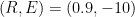 . Iterating will then decrease
  without limit: it will take off to negative infinity.
From the unstable state , that is, the system will take off when nudged to either negative or positive infinity in accordance with the nudge’s direction.
As I explained in the head post, nonlinear-system behavior is somewhat different, but the linear-system behavior gives you the basic idea.
Joe Born:
Ah. Helpful!
Thanks. But, still leaning toward CM and will interested to hear about his upcoming presentation.
JRF.
Low solar drives warm ocean phases which reduces cloud cover in the mid latitudes and increases cloud cover in the Arctic. Huge negative feedbacks. The globe would have cooled from 1995 without the AMO acting as a negative feedback to declining solar wind pressure.
Negative feedbacks are not just things that work against another, but one has to cause the other. So saying solar is a “feedback” implies that solar is caused by global temperature. So, if solar is changing cloud, that is not a feedback to the system but a driver.
So your second sentence would be:
“The globe would have cooled from 1995 without the AMO acting as a driver warming the temperature in the face of the cooling effect of declining solar wind pressure.”
As to that statement … all I can say, is that so far there is no evidence of sustained cooling beyond the expected** cooling after the 2016 El Nino
**OK, only sceptics expected it to cool. The idiots in the Climate Cult didn’t.
I did not say solar was a feedback, hello? The warm ocean phases and cloud clover changes are the negative feedbacks to changes in indirect solar forcing, i.e. to the decline in solar plasma pressure/temperature since 1995.
I did not expect sustained cooling after the 2016 El Nino, as I had predicted a continuation of increased El Nino conditions beyond 2016, about 6 years ago on this blog.
**Don’t misquote me.
What Monckton did was show what the elephant looked like if its trunk wasn’t wiggling.
What’s the difference between a marginal tax rate and an average tax rate?
The average rate takes all the prior income and taxes into account.
The marginal tax rate looks at the change in income and the change in taxes.
Assume a relevant range of the U.S. Income tax rates.
Using the average rate hides the bad news if you add some income and your tax rate is 35%. The reality of it is, most accountants would agree the government smacked you for more than a third of the additional income.
I wonder if that’s what happened?
Fixated on anomaly data?
The bottom line, it is all the temperature, or CO2 level, or humidity that has to be processed because that is how nature works in its attempt to seek equilibrium (not that it ever gets there before something has changed).
Joe,
Your equations are very similar to ones I have posted on some Monckton threads, except I am sticking with a 1/4 power law. Essentially it is an implicit equation (therefore solved numerically) which says that temperature T is a function of sums of forcings Fi one of which depends on T itself:
T(F) = (F/(εσ))1/4 (2)
Now total forcing F is the sum of F1 + F2 + F3, where F3 depends on T. So
F = F1 + F2 + F3(T(F))
I then derive sensitivity S to doubled CO2 as
S = 3.7 / (4εσT(F)^3 – F3’(T(F)))
So the denominator implies that a tipping point is possible. I then use real world annual observations from Ramanathan & Inamdar (2006) to deduce a plausible value for F3′ of 3.53 and S = 2.12K.
This non-linear theory, which is physically more justifiable than for temperature to feed back directly on itself, gives a significantly higher S (2.1K) than Monckton gets (1.1K), but not too scary. I should like to publish this in a journal, but have lacked the motivation to work hard enough to that end. I could send you a draft if you wished.
I, too, ran the model with 1/4 power, and in a sense it was more interesting. But for the head post I adopted the fractional power 0.37 for two reasons.
The main reason was to match the oft-quoted current-concentration open-loop-gain value of 1/3.2. That’s what I meant above by “a nod toward the real-world difference between the surface temperature and the effective radiation temperature.”
An ancillary reason was that with 1/4 power the instability at absolute zero was more pronounced. That made the gap at absolute zero detectable enough to require that I provide an explanation. As you might have inferred from the above discussion’s caliber, almost no one would have comprehended that explanation. So the power I chose above had the incidental benefit of sparing me a pointless exercise.
As to a paper, I have no academic pretensions. I’m nearing my sell-by date, and even in my working life I was just a workaday lawyer, part of that vast army of gray men who make their living by keeping the gears of commerce oiled.
I bestirred myself in this case only because I’m a citizen, because a significant part of the skeptic community seems to have been taken in by a clearly incorrect understanding of control-systems theory, and because I happen to know that discipline’s rudiments. (And make no mistake; the head post deals with only the most rudimentary of its rudiments.)
That said, I’ll mention that I have reservations about your equation’s use of . Let me emphasize again that I’m no climate scientist. And I may misunderstand what you mean by
  and
and  , so the following observation may be meaningless.
But my opinion, as the post said, is that “temperature almost certainly isn’t a single-valued function unless that function’s argument is a vector of forcing components instead of the scalar total thereof we’re assuming here.” In other words, I was alerting readers to the fact that I was averting my eyes from the errors attendant to treating a function of a vector as a function of the scalar total of its components.
For example, suppose that, for some ,
,  and
and 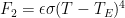 . Then treating the open-loop function as
  would imply that
  has a one-to-one mapping to distance along a specific but only implicit trajectory through the
  plane. Now, that’s in essence what the head post did tacitly: if forcing is indeed properly treated as a vector of components whose effects differ, then by treating vector forcing as a scalar sum of its components I was tacitly assuming a trajectory through the forcing-vector space.
In the case of the head post, I simply avoided this discussion, which would have required more physics that I’m sure of and anyway would have been lost on this audience. But by naming the components explicitly you may instead need to deal with that complication. Or maybe I just don’t understand your approach.
Anyway, those are all the thoughts I have on it. And, again, my purchase on that corner of the problem is somewhat tenuous, so take this comment for what it’s worth.
Joe, thanks for the reply. It is always hard to know whether to post more detail, which can put some people off, or to post less and then be improperly understood.
Anyway, you already guessed that F is for Forcing, in W/m^2. T(F) is the Stefan-Boltzmann 1/4 power equation. The things you couldn’t guess are that F1 is the solar input, F2 is the total CO2 forcing, and F3 is the temperature-dependent effect of water in all its guises, especially albedo from ice and downwelling infrared from water vapour.
Though my equation is implicit for T, it does have well defined solutions which can be found by computer iteration. In this “zero dimensional” model I, like Monckton, go along with the assumption or approximation that T is a meaningful quantity, but do not go along with the linear feedback theory of T on itself, because manifestly one can add energy fluxes (F) in a meaningful physical way, but one cannot add temperatures.
Perhaps your posting will reignite my desire to head for publication, but I am currently distracted by a totally different area of mathematics, not to mention enjoying retirement!
Rich.
Actually, it appears that I was nearly correct about and
and  , but I flubbed the math on
  .
.
My guess was that is the type of forcing that, as solar radiation does, increases the equilibrium top-of-the-atmosphere outgoing radiation, and
  is the type that doesn’t, as greenhouse gases don’t. Without greenhouse gases, the outgoing radiation is
  , where
  is both the effective radiation temperature and the radiation-average surface temperature.
If greenhouse gases suddenly appeared in the atmosphere, radiation out would suddenly drop by , where
  the value to which the radiation-average surface temperature will rise as equilibrium is restored.
Unfortunately, would include both forcing types: albedo decrease would increase the outgoing radiation, but water vapor as a greenhouse gas would not.
Just one small point about F2 (GHG) versus F1 (solar). The surface of the Earth doesn’t care whether a watt per square metre arrives as part of F1 or F2. Much as Monckton says that feedback doesn’t care which of the 280ish degrees it is responding to, only the total.
Though one can’t rule out differing effects from the wavelengths of the F1 and F2 inputs, especially regarding penetration into water, but mainstream climate science ignores that for the purposes of simple zero-dimensional models such as these.
I agree; the surface doesn’t care. At least for purposes of discussion, that is, it’s reasonable to assume that the large-signal feedback depends only on the entire surface temperature. And, of course, that’s what I assumed in the head post, ignoring any problems that basing derivations on the concept of a large-signal forcing quantity may raise.
I nonetheless think the concept is problematic and that dealing with the different forcing flavors may force you to face its problems. As I said, I ignored the problem myself and haven’t thought it through. But the three rough-and-ready attempts below to assign a forcing value to a surface temperature will suggest why I have reservations.
To me they seem to show that the absolute temperature would depend not just on what the total of the large-signal forcing quantities is but also on how that total is divided among the forcing types. Worse, it may also depend on the path by which the state was reached.
Forcing Calculation A:
Starting at absolute zero with no greenhouse gases, we turn the sun on, with intensity high enough that average insolation is , which is therefore the initial imbalance at the top of the atmosphere: it’s our first forcing value
  .
.
We then get some coffee while the earth equilibrates, i.e., until the radiation out equals the radiation in. When it has, the surface temperature is . (That’s the surface’s effective radiation temperature; we’re ignoring complications like Hölder’s inequality, diurnal variation, etc.) And, since there are no greenhouse gases, that’s also the emission temperature. We’ll refer to the system’s state as its (emission temperature, surface temperature) ordered pair: the final equilibrium state is
  . And ostensibly
  is the large-signal forcing value corresponding to
  .
.
As we’ll see by way of Forcing Calculation B, though, the large-signal forcing that corresponds to that surface temperature seems to be different if the emission temperature isn’t the same.
Forcing Calculation B:
Starting at absolute zero with no greenhouse gases, we turn the sun on, but with less intensity this time, causing an initial radiation imbalance of ,
,  , so that's the forcing
  associated this time with sunshine:
Once the earth equilibrates we add a bolus of greenhouse gas great enough to reduce the outgoing radiation by:
where . So
. So  is the forcing associated with greenhouse gases. (We won't distinguish here between direct and feedback forcing.) When the earth re-equilibrates, the surface temperature ends up equal to
  as it did in the previous calculation. (Actually, the initial emission-temperature reduction
  required to achieve that result probably isn't exactly
  , but I'll ignore that for this rough calculation.)
Note that this time the forcing that corresponds to
  is given by:
instead of the value the previous calculation gave it.
And Forcing Calculation C will suggest that large-signal forcing may depend not only on the state but also on the path taken by the system to reach that state.
Forcing Calculation C:
Starting again at absolute zero with no greenhouse gases, we turn the sun partially on, causing an initial radiation imbalance of ,
,  , so that's the forcing
  associated with turning the sun on part way:
After the earth equilibrates, we add the greenhouse gases, this time initially causing an imbalance of only , where
  . The forcing
  associated with greenhouse gases this time, that is, is given by:
After the earth reaches equilibrates again, the surface temperature is . Then we dial the sun up further to irradiate the earth at
  . That makes the forcing
  added by dialing the sun up further equal
so the total solar forcing is given by
in Forcing Calculation C the solar component is the same as in Forcing Calculation B.
Now, here I'm going to make something of a leap and say that after the earth equilibrates yet again the surface temperature will equal even though before the sun was dialed up further the difference between surface and emission temperatures was only
  , not
, not  . I'll leave you to judge how plausible that is.
If it's true, though, we have a final state state with Forcing C that's the same as Forcing B's final state: . But the forcing
  associated with the greenhouse gases in this case is different, so the forcing calculated this time for the exact same state
  is different:
In short, the concept of a large-signal forcing quantity strikes me a problematic. By basing calculations on perturbations rather than entire quantities, the conventional feedback representation finesses around this difficulty, and I think validly. I don't think that can be said of Lord Monckton's temperature-input view, which, moreover, is unphysical. If you return to this question, though, I'll be interested in what you come up with.
Again, the head post just ignores this problem. And I've just whipped this comment out for whatever value you think it has. Obviously, it doesn't come within shouting distance of rigorous.
Joe (July 21 2:36pm), that is some interesting mathematics, but you asked for my judgment on some plausibility. I have two problems with the maths you presented. (For celerity I’m going to use d in place of Delta and drop epsilon times sigma – we know where that goes in.) First is that you used
From there you will get (T1-dTC)4 = F1C1-F2C, and that doesn’t give you a direct equation for T1+dTC. To fix this I think you need to use F3C = (T1+dTC)4-T14 instead. Then with FC =F1C+F3C we get an associated temperature
T(FC) = (TE4 + (T1+dTC)4 – T14)1/4
~ (TE4 +4T13dTC)1/4
~ TE (1+T13dTC/TE4 )
= TE + (T1/TE)4 dT, ignoring terms in dTC2
This perturbation does not equal your dT. So I can’t really accept your conclusions…
Sorry, copying and pasting from Word did not preserve subscripting. Here’s a better ASCII version.
Joe, that is some interesting mathematics, but you asked for my judgment on some plausibility. I have two problems with the maths you presented. (For celerity I’m going to use d in place of Delta and drop epsilon times sigma – we know where that goes in.) First is that you used
From there you will get (T_1-dT_C)^4 = F_1C1-F_2C, and that doesn’t give you a direct equation for T_1+dT_C. To fix this I think you need to use F_3C = (T_1+dT_C)^4-T_1^4 instead. Then with F_C =F_1C+F_3C we get an associated temperature
T(F_C) = (T_E^4 + (T_1+dT_C)^4 – T_1^4)^(1/4)
~ (T_E^4 +4T_1^3 dT_C)^(1/4)
~ T_E (1+T_1^3 dT_C/T_E^4 )
= T_E + (T_1/T_E)^4 dT, ignoring terms in dT_C^2
This perturbation does not equal your dT. So I can’t really accept your conclusions…
Well, as I said, I wanted to spare myself having to think this issue through; that’s (part of) the reason why I simply accepted Lord Monckton’s entire-quantity framework for the sake of argument. So my thinking on it is still half-baked.
In other words, you may be right in saying (or at least I think this is what you’re saying; a passage seems to be missing from your comment) that my rationale for the value I gave the third calculation’s greenhouse-gas forcing is faulty:
For what it’s worth, though, I’ll just make that rationale explicit.
At the initial equilibrium after the sun has partially been turned on the earth’s emission temperature is : it’s radiating
  into space. And that’s exactly what the earth is absorbing from space.
Now enter a slug of greenhouse gas. Initially the surface is still radiating what it receives from space, but the greenhouse gas intercepts some of that re-radiation, so from space’s viewpoint it’s as though the earth is no longer radiating from the temperature- surface but rather from an altitude where the temperature is a cooler
  : space now receives only
  , so there’s initially an imbalance
  .
.
That’s the forcing value I associated with adding the greenhouse gas, and I assigned the symbol
  to the quantity
  .
.
Taking the baby steps to which the limitations of my once-passable algebra ability now make me resort produces the following:
Again, you may be right that it makes more sense instead to base the calculation on the radiation from the surface rather than from the effective radiation altitude, although I haven’t yet been able to warm to that approach. Like you, though, I have other fish to fry at the moment, so I doubt that I’ll be getting to the bottom of this any time soon.
we must first understand the different physical processes of feedback before writing math equations :
if we come back 20k years ago, Earth was covered by ice (down to New York), so ice albedo plays an important positive feedback, secondly, green house effect is about proportional to earth IR and third oceans contain main resources of CO2 which is released to atmosphere depending of their temperature .
So when astronomical factors (excentricity of orbit + obliquity ) brought additional solar irradiance , the combination of those feedback effects has led to Holocen peak period 8000 years ago , and now earth is going back slowly to a new glaciation period following Milankovitch cycles. We can easily understand that when ice glacier has melt, this particular factor is becoming less important and don’t forget the non linearity of green house effect.
We can add the cosmic rays impact on cloud albedo (CERN experience) and other oceans cycles (AMO, PDO, ENSO).
When the equation of natural cycles has been written and compared to real data , we can add anthropogenic CO2 to get final relationship .
Don’t put horses behind !
For last 40 years of TOA short waves measurement , satellites were unable to give accurate data about albedo , only 1% or 3 watts/m2, so greater than we can expect from anthropogenic effect , also we don’t know the albedo change during Holocen (only by ice observations last centuries).
We clearly miss correct data to build an effective model and propose serious forecast …
Precisely. Your math doesn’t matter when you do not understand the system. The math geeks love this stuff, they revel in the numbers being crunched, but to the rest of us it is simply mathturbation. Nothing, is being created.
So many words spent answering supposedly simple question: according to the control theory, does feedback loop responds to the entire input signal or to the perturbations only? I cannot believe an answer is so complicated and unconvincing as presented in this article. Clear, simple and concise answer should be the first step. The next step would be: assuming that Lord Monckton has control theory right does it apply to the climate model? Maybe it does not. Maybe, for instance, climate science never uses such feedback mechanism thus Our Lord criticism is misdirected. That would be an interesting line of enquiry. Instead, we’ve got ‘thousands of words novella’ basically saying ‘it is complicated’. This very fact suggests that Our Lord may have hit the soft belly of the climate models.
You’re right; it is very simple. As I’ve explained more than once, Lord Monckton’s theory simply boils down to bad extrapolation: he uses the average slope rather than the local slope for extrapolation.
High-school analytic-geometry students know using the average slope is wrong. Here’s an example of where I’ve explained it: https://wattsupwiththat.com/2019/06/03/reporting-the-fraudulent-practices-behind-global-warming-science/#comment-2715071.
Unfortunately, Lord Monckton has complicated the issue; he has convinced people like you that there’s something about feedback theory that requires abandoning everything we know about extrapolation. He’s does this by causing you to focus on red herrings like, “according to the control theory, does feedback loop responds to the entire input signal or to the perturbations only?”
The truth of the matter is that nothing turns on that question; he’s wrong whichever way you look at it. So the post above assumes his entire-signal rule and comes up with high ECS anyway.
And, sorry, but actually working through feedback is complicated.
But, if you’d rather not work through it, here’s a suggestion. Just search the head post for the paragraph that contains “blows up” and do the iteration described there to see for yourself whether he’s right or I am about his“global cooling” interpretation. If you’re capable of a little arithmetic, the answer will be clear.
Hey Joe,
He’s does this by causing you to focus on red herrings like, “according to the control theory, does feedback loop responds to the entire input signal or to the perturbations only?”
I think not. That’s the valid question. Granted, our Lord can get a wrong answer. Even if he’s right as far as control theory is concerned that may be simply not applicable to the filed of climate modelling. That might be all true but it is not blindingly obvious from your article. In all fairness it is not even vaguely obvious. Putting aside ‘thought experiments’ and mystification of the feedback loops I can see at least two options to verify question in the subject. First is to build a test rig with appropriate feedback loop and simply measure input/output values plus values between different components of such rig. I believe our Lord and his co-authors build few such rigs and claim that empirical findings confirm their position. If that can be reproduced by different researches that should settle the question. Second, is to build a virtual rig using high-quality software as Matlab control system toolbox and do the same checks.
I reckon our Lord is going to give a presentation in the Heartland Institute about this very issue quite soon. Looking forward for more details!
Elsewhere on the thread some commenters found what appears to be a draft of Lord Monckton’s paper, including specifications of the “test rig” and test results.
It turns out that, contrary to what the authors contend, the “test rig” shows what I’ve always said it would: the “official climatology” approach of using perturbations works just fine, thank you, whereas Lord Monckton’s approach works only in the linear case. Just as a high-school analytic-geometry student could have told us.
By the way, although I haven’t so much as touched a soldering iron since the Vietnam War, I have indeed written a virtual “test rig,” and it demonstrated that Lord Monckton’s approach fails. Unfortunately, the proposed post by which I would have shared it with all and sundry got spiked.
Hey Joe,
Elsewhere on the thread some commenters found what appears to be a draft of Lord Monckton’s paper, including specifications of the “test rig” and test results.
Where is it? And have someone actually built a rig, according to our Lord specs, and has proven that it behaves differently than our Lord claims? I’d love to see that. My impression is that someone imagines how such rig would work and then, based on such rich imagination, claims ‘refutation’ of Monckton’ thesis. I’m afraid they have to offer something more tangible than pure imagination.
By the way, although I haven’t so much as touched a soldering iron since the Vietnam War, I have indeed written a virtual “test rig,” and it demonstrated that Lord Monckton’s approach fails.
No pressure to build a rig by yourself – I reckon someone eventually will do so to validate our Lord’ results. That should settle the matter. And I reckon is not difficult to build such device. And I reckon it will show exactly what our Lord claims. Maybe that’s why so far his critics offer mainly ‘thoughts experiments’ instead of hard evidence.
I touched control theory in the past only lightly but I’ve had a quick look on the industry-standard control software libraries; more exactly on a textbook example (Feedback Systems by Astrom and Murray, 2008) of a vehicle cruise control system with a full nonlinear model of the vehicle dynamics and a proportional integral controller. From what I can see from the code is you pass to the feedback module the whole input, in this case total vehicle velocity:
—————-
# Figure 1.11: A feedback system for controlling the speed of a vehicle. In
# this example, the speed of the vehicle is measured and compared to the
# desired speed. The controller is a PI controller represented as a transfer
# function. In the textbook, the simulations are done for LTI systems, but
# here we simulate the full nonlinear system.
[…]
for m in (1200, 1600, 2000):
# Compute the equilibrium state for the system
X0, U0 = ct.find_eqpt(
cruise_tf, [0, vref[0]], [vref[0], gear[0], theta0[0]],
iu=[1, 2], y0=[vref[0], 0], iy=[0], params={‘m’:m})
t, y = ct.input_output_response(
cruise_tf, T, [vref, gear, theta_hill], X0, params={‘m’:m})
———————–
input_output_response function computes the output response of a system (vehicle velocity, t) to a given input. First argument cruise_tf is the return value of the feedback function:
————
# Construct the closed loop control system
# Inputs: vref, gear, theta
# Outputs: v (vehicle velocity)
cruise_tf = ct.InterconnectedSystem(
(control_tf, vehicle), name=’cruise’,
connections = (
(‘control.u’, ‘-vehicle.v’),
(‘vehicle.u’, ‘control.y’)),
inplist = (‘control.u’, ‘vehicle.gear’, ‘vehicle.theta’),
inputs = (‘vref’, ‘gear’, ‘theta’),
outlist = (‘vehicle.v’, ‘vehicle.u’),
outputs = (‘v’, ‘u’))
———–
where again input to this feedback function is the velocity (vref), gear and theta (i.e. pitch angle of a vehicle). Thus input to the feedback function is the whole velocity, whereas output (v) is velocity after disturbances (as uphill angle). Then, that output (again velocity) is passed to the function calculating change in velocity of a vehicle going uphill.
That is a settled, established engineering science I’m able to – with a little bit of effort – follow. And this established science clearly and swiftly confirms our Lord’ thesis. Compared to this your article is hardly digestible to me. Nothing personal of course. I’m sure that my mental bandwidth is not wide enough to fully accommodate those truths. You guys are so brave, handsome and intelligent. Still, would be nice to have a reliable and accessible by little, simple brains critique of Lord Monckton’ thesis.
I beg your pardon; I see I failed to reply.
I won’t attempt to tease out the relevance of the text excerpt, but the draft paper I referred to can be found at https://cornwallalliance.org/wp-content/uploads/2018/01/sen.pdf
Here’s a simple way to visualize the condrum Mr. Born is illustrating. The classic problem in multivariate (state variable) control is the broom balancer problem; an analogue for balancing a rocket on its engine.
If one observes a rocket risking smoothly into the sky, are the control systems either (a) applying a few butterfly kisses to the flight surfaces and engine gimbals to keep the rocket rising smoothly towards the heavens or (b) are the servos working feverishly hundreds of times per second to keep all that tonnage (of constantly dimishing weight no less) balanced on the controlled deflagration thundering out the engine bells?
Which answer is (more) correct isn’t important. The point here is that one cannot discern that truth observing the rocket rising smoothly upwards. Could be one, the other, some combination of the two or something entirely different. Mathematically, this inability to discern the system’s internal behavior from measuring the outputs is called observability.
Taking an input and output data set, one can conjur any number of transfer functions (high gain, low gain, strawberry, lemon-lime, etc.) and fit it’s coefficients to the data. As with any curve-fitting exercise, one is often advised to keep the coefficient count within the available degrees of freedom.
One can make many excellent arguments for low gain, near invariance, etc. For reasons having nothing to do with the transfer function mathematics, I’m sympathetic to many of those arguments. Do I think there is a tipping point waiting for use just a few more tenth’s of a degree out there? No, I don’t.
However, if the argument is that the transfer function model math is proof that the climate forcing feedback is agreeably low, then the argument fails precisely as illustrated by Mr. Born. Lord Monckton has recalculated the GHG feedback observing the absence of an important element which results in a much reduced forcing feedback. Nothing wrong with that approach given the working hypothesis of the original models.
However, other workers can simply shovel other terms into the model which drives the feedback forcing upwards. Is that right and do I necessarily agree with it? Nope, but illustrates that the original model’s approach is flawed as proof of AGW. One can rub-on first princples arguments on why certain terms should/should not be allowed into the model; but, in the end the model cannot be used to feret-out which terms are worthy and which are neglible. The math works-out in all of the cases.
My appreciation to J.Born for working it out.
The more I look at this the more this experiment seems confusing. There is a line that says: “In this circuit, the polarity of the output is always inverted: however, since this inversion has no effect on the absolute value of the output, for clarity it has been ignored in all tables.”
The sign of the output would seem to be very important to me. As you decrease the negative feedback, thus increasing the inverting gain of the amplifier, you increase the output of the system in a negative direction. This would be like saying that increased CO2 causes a *drop* in temperature, not an increase.
I don’t hold that “test rig” demonstration in high regard, but it can’t really be criticized for asking that we ignore that inversion. It establishes exactly what it would have without the output inversion; the inversion was just an implementation convenience.
I did the same thing in a previous post, and the readership got distracted by the polarity then, too. So when I wrote a virtual “test rig” of my own (which didn’t get into a head post) I took the extra step of re-inverting.
Joe, I think we’ll just have to agree to disagree. My old analog computer professor was a stickler for following polarities through. If you didn’t then trying to model all kinds of things didn’t work out correctly for modeling reality.
If you are trying to generate a circuit model describing the effect of increased/decreased CO2 then using the inverting input of an op-amp is not a proper model. In a holistic approach this circuit element will be combined with other circuit elements that represent other sub-systems in the atmosphere. If you just ignore polarities of each element then you’ll never get a proper representation of reality.
Just sticking an inverter on the output may or may not correct the problems when multiple circuit elements are combined.
I hesitate to get too deep into this but grounding the non-inverting input and summing everything at the inverting input is probably not the best way to do this. I would have used a single op-amp as a comparator where E0 would be fed into the non-inverting input and the negative and positive feedback loops fed into the inverting and non-inverting inputs.
I’m still not sure what all this was meant to prove. You could have done the same thing by just making R2 a variable resistor (with all the circuit elements of op-amp 2 deleted) and measuring the change in the output as R2 is varied! So what does that prove exactly?
My main problem with the IPCC’s, Lord Christopher’s and Joe’s investigations into climate feedback is simple.
I think that the climate system has a governor. A governor is is a mechanism that applies either positive or negative feedback to maintain a system near its operating point. It is not feedback. It is a separate system that controls the feedback.
In other words, you guys are making the same mistake as using simple linear feedback equations to attempt to analyze a car’s “cruise control” system. A cruise control is a governor, using both positive and negative feedback to maintain the car at a given speed regardless of changes in the load.
And AFAIK, such a system cannot be analyzed using the equations of simple linear feedback, whether they are the IPCC’s equations, Lord M’s equations, or Joe’s equations.
Best to all,
w.
My main problem with Mr. Eschenbach’s comment is the failure it betrays to grasp the concept of accepting a proposition for the sake of argument.
However crabbed his definition of feedback may appear to some of us who have studied control-systems theory in depth, I actually have considerable sympathy for aspects of his “governor” theory. But the question before the house isn’t tropical thunderstorms. It isn’t whether Lord Monckton or I—or even the IPCC, for that matter—believes that the climate is a linear scalar system. It isn’t even whether I believe there’s such a thing as equilibrium climate sensitivity (“ECS”).
It’s whether Lord Monckton has proved mathematically, as he says he has, that high ECS values result from a failure to recognize that “such feedbacks as may subsist in a dynamical system at any given moment must perforce respond to the entire reference signal then obtaining, and not merely to some arbitrarily-selected fraction thereof.” And in demonstrating that Lord Monckton’s proof fails, I assumed Lord Monckton’s entire-signal rule and scalar framework only for the sake of argument, just as it was only for the sake of argument that Lord Monckton was assuming what he says were elements of “official climatology’s view.”
I demonstrated his proof’s failure by obtaining under those assumptions not only a high ECS value but also a tipping point. But that didn’t mean I believed those assumptions to be true. Accepting them for that purpose was therefore not a mistake.
So even if I had employed linear feedback in the process—and, in fact, I didn’t—Mr. Eschenbach still would simply be wrong to contend that I was “making the same mistake as using simple linear feedback equations to attempt to analyze a car’s ‘cruise control’ system.” And that’s even if we accept his view—for the sake of argument—that “a mechanism that applies either positive or negative feedback to maintain a system near its operating point . . . is not feedback.”
What you are describing is commonly known as PID control of a process. PID stands for Proportional, Integral, and Derivative. You establish a set point you want for a process and measure the output of the process and feed those into a summing junction which generates an error signal. The error signal (perhaps multiplied by a gain factor), the integral of the error signal, and the derivative of the error signal are fed into a second summing junction to generate a control signal used to correct the process toward the set point.
Since you have only one variable involved, the output of the process, each of the individual terms of the PID control is pretty easily analyzed.
This type of control is probably not applicable to the climate because there is no “set point” that can be established as a start point as you can do with the cruise control of a car.
Tim Gorman July 20, 2019 at 5:29 am
Thanks, Tim. Actually, I had in mind something more like James Watt’s flyball governor, which is simply a P controller, not a PID controller. However, most folks are unaware of what a flyball governor is, so I used a cruise control as my example. It is indeed a PID controller, as you point out.
Actually, the “set point” over the ocean, which is where much of the controlling goes on, appears to be on the order of 26°C … here, for example, is cloud coverage versus surface temperature:
And here is cloud top altitude (a proxy for thunderstorm formation) versus surface temperature:
See my posts Glimpsed Through The Clouds and Albedic Meanderings for further discussions of the set-point question.
Best regards,
w.
A flyball governor or an air-vane governor (like on a small lawnmower engine) still both have set points to control what happens to the engine speed, even if they only implement the P part of PID.
If the Earth has a set point mechanism useful in controlling anything then it doesn’t work very well or we wouldn’t see such monumental swings in the Earth’s environment like ice age temperatures and inter-ice age temperatures.
While cloud coverage over the ocean has some impact on controlling the temperature of the ocean there are also other inputs which impact it as well (e.g wind, seasonal variation, ocean currents, etc). A true representation of the climate would have multiple inputs to the summing junctions, not just one.
Remember, a linear equation is not just of the form ax+b = 0. For example, it can be of the form ax+by+cz+eu+fv= 0 where a,b,c,e,f are all constants and some may be positive and some may be negative. You still get a straight line from each form of the linear equation. From the shape of your curves it appears that some form of PID control would have to be involved, especially the I part since that can generate a non-linear result for the feedback. I’m not sure how a climate process could generate a non-linear control signal.
Tim Gorman July 20, 2019 at 1:06 pm
“Doesn’t work very well”? The temperature of the earth varied only by ± 0.3K/288K = ± 0.1% over the entire 20th century. Yes, any control system can be overwhelmed by e.g. a Milakovich cycle, but that does NOT mean it doesn’t work very well.
Heck, you’re a controls guy—how good is a system that keeps the temperature within ± 0.1%? And please, don’t ascribe that to “thermal mass”, not in a system where the temperature of nearly every spot on the earth varies hourly, daily, and monthly by many degrees … especially a system which is running some fifty degrees C about what would be expected from Stefan-Boltzmann calculations.
The control system of the earth is like the control system of a house with a thermostat—it is temperature threshold based. Yes, there are lots of inputs to your house temperature, the wind, the humidity and the like … but the threshold is not responding to anything but temperature.
And when you look at the graphs I just posted above (and I have lots more showing the same 26° threshold), it’s evident that temperature is overwhelmingly the main input to the threshold, and the other phenomena you mention seem to average out.
Seems to me that any threshold-based control system, like your furnace thermostat, generates a non-linear control signal. And with the climate, there are no less than four succesive temperature thresholds, each of which is associated with a new emergent phenomenon, viz:
• the onset of Rayleigh-Bénard circulation of the lower atmosphere
• the onset of the cumulus cloud field
• the onset of the thunderstorm regime
• the aggregation of thunderstorms into larger groups, e.g. squall lines.
Since each of these increase the surface cooling, the total system is assuredly non-linear.
There’s also the onset of Rayleigh-Bénard circulation of the upper ocean, which is also temperature based, although in the opposite direction—it emerges when the temperature gets below a certain threshold, and it acts to increase the heat loss from the mixed layer.
Finally, thunderstorms have “overshoot”—they cool the surface to a temperature BELOW the temperature at which they emerge. As you undoubtedly know, such overshoot is important in controlling a lagged system like the earth’s temperature.
Best to you and yours,
w.
““Doesn’t work very well”? The temperature of the earth varied only by ± 0.3K/288K = ± 0.1% over the entire 20th century. Yes, any control system can be overwhelmed by e.g. a Milakovich cycle, but that does NOT mean it doesn’t work very well.”
A control system that is overwhelmed is not much of a control system. If external inputs determine actual conditions some of the time then why don’t external inputs determine actual conditions at other times?
“but the threshold is not responding to anything but temperature.”
This is an *assumption” you are making. I see nothing that actually validates the assumption. All your graphs shows is that ocean temps are an input to cloud formation. That doesn’t prove a direct correlation to anything else.
“it’s evident that temperature is overwhelmingly the main input to the threshold, and the other phenomena you mention seem to average out.”
Ocean temp might be the main input to cloud formation but that doesn’t mean ocean temp is a direct control of anything else. And how do we know that the other phenomena average out?
“Seems to me that any threshold-based control system, like your furnace thermostat, generates a non-linear control signal.”
Sort of I guess. It is actually binary. It is either on or off. There are no intermediate values produced. There are no second order elements introduced into the process. It can be considered a a piecewise linear function as discussed below.
“Since each of these increase the surface cooling, the total system is assuredly non-linear.”
If different feedback mechanisms come into play at different times in the process and each segment is linear then the feedback mechanisms can be analyzed as part of a piecewise linear function. In fact, that is what your temp vs cloud graphs appear to be, a piecewise linear function, some segments having a positive slope and some having a negative slope.
Tim Gorman July 20, 2019 at 4:35 pm
First, it gets overwhelmed once every 100,000 years. Seems pretty solid to me. Have you designed any control systems that only get overwhelmed once in a hundred millennia?
Second, ANY control system can get overwhelmed. My air conditioning can get overwhelmed by extreme hot temperatures. My furnace may not get up to the set temperature if the weather dips below 0°F. My cruise control can’t keep my car within speed specs on a steep downhill. Surely, as someone familiar with control systems, you must know this?
Seriously? If you can’t answer this you’re not much of a control person.
I didn’t say that there wasn’t some kind of correlation to something else. I said, and the graphs show clearly, that once the temperature of ~ 26°C is exceeded, you enter an entirely new regime.
If they didn’t average out, then there wouldn’t be the clear and obvious “knuckle” in the graphs at 26°C.
“Piecewise linear”? Almost curve can be considered to be “piecewise linear”. I fear that’s hardly an objection.
“Piecewise linear” is just one kind of non-linear. You are grasping at semantic straws.
w.
“Second, ANY control system can get overwhelmed. My air conditioning can get overwhelmed by extreme hot temperatures. My furnace may not get up to the set temperature if the weather dips below 0°F.”
These are not failures of the control system. These are failures of the process being controlled!
““Piecewise linear”? Almost curve can be considered to be “piecewise linear”. I fear that’s hardly an objection.”
Nope. A curve is a curve, it has higher order elements in its function. A piecewise linear function is made up of linear segments. No higher order elements in any segment.
““Piecewise linear” is just one kind of non-linear. You are grasping at semantic straws.”
I’m sorry. Piecewise linear functions are a defined mathematical entity. Consider a process where water is added to a material and the temperature must be maintained at 110degF to ensure proper mixing but once the mix is done the temperature must be maintained at 60degF to ensure proper curing. One control system handles the heating element and a separate control system handles the cooling element. Both segments involve a linear control system but the overall process has a piecewise linear control function.
I am certainly not a control system expert. But I was involved a number of years ago in a project where several separate control systems were an integral part of the overall system. I did learn some about control systems at that time.
Tim Gorman July 21, 2019 at 5:40 am
So when the earth’s temperature control system, which has held the temperature within ± 0.5% for over ten thousand years, is overwhelmed by the unrelenting cold due to Milankovich ice age cycles, that’s a “failure of the control system”.
But when my home furnace is overwhelmed by unrelenting cold, that’s a “failure of the process being controlled”.
If that is the level at which you wish to debate, I’m gonna have to pass. I cannot deal with that level of disconnect.
Best regards,
w.
“So when the earth’s temperature control system, which has held the temperature within ± 0.5% for over ten thousand years, is overwhelmed by the unrelenting cold due to Milankovich ice age cycles, that’s a “failure of the control system”.”
*I* never said that the ice ages are the fault of the control system. I said it was the fault of the system being controlled not being able to handle the load it is being asked to handle.
It is not a problem with the feedback system associated with the Earth’s climate if enough energy input is not available to keep the Earth from having an ice age. The Earth doesn’t generate energy, it is an input to the system. If the fuel system in your car can only provide enough fuel for the car to go 50mph you can mash the accelerator to the floor hoping to go faster but it won’t happen. You can set your cruise control to 80mph but your speed will never get there. That’s not the fault of the accelerator or the cruise control. It’s the fault of the drive train system.
It’s exactly the same with the Earth. If it doesn’t get enough energy from the sun no control system possible will change that fact.
There is a set point for the system. It is energy in must equal energy out.
Add a little more energy from the sun and the earth must warm up and it’s converse is also true. However the effect of the feedback can exaggerate the temperature response but it still must balance out eventually.
Thanks, Joe. I do “grasp the concept of accepting a proposition for the sake of argument.” However, in this case I’m questioning its utility.
Perhaps I can illustrate by example. Someone says “I think that the earth’s climate is ruled by the effect of gamma rays on man-in-the-moon marigolds”.
Now, you can accept that proposition “for the sake of argument” … but I doubt greatly whether you’ll ever learn much useful from doing so.
As to your claim that my “definition of feedback” is “crabbed”, please quote where I defined “feedback”, as I have no memory of doing so.
Best regards,
w.
“Please quote where I defined ‘feedback’, as I have no memory of doing so.”
Me neither. But whatever it is, it excludes a “mechanism that applies either positive or negative feedback to maintain a system near its operating point.” Mine wouldn’t.
And I, too, would “doubt greatly whether you’ll ever learn much useful” from assuming for the sake of argument that “The earth’s climate is ruled by the effect of gamma rays on man-in-the-moon marigolds” if that’s all someone had said. But, of course, that’s not all there is to it.
To make your analogy more apt, the theorist would also need to have said, “Once that point—which is well established in control theory but has, as far as we can discover, hitherto entirely escaped the attention of climatology—is conceded, as it must be, then it follows that equilibrium sensitivity to doubled CO2 must be low,” and also have said his theory’s “a way—and I’m going to use the word compel—to compel the assent” of those who think it’s high. .
And a further part of the analogy would need to be that because of that conclusion:
—The Heartland Institute had him present that theory at the 12th International Conference on Climate Change.
—In the presentation he implied that someone who’s now a member of the National Security Council commented favorably on his theory.
—A Youtube video of the talk was billed “Monckton’s Mathematical Proof; Climate Sensitivity Is Low.”
—In another Youtube video the editor of The New American magazine introduced that theory as “an incredible new development” and a “game changer,” that “is going to make a huge difference in everything we know about climate change.”
—Roy Spencer’s blog ran his theory.
—There was a call for crowdfunding support of legal action against scientific journals’ refusal to publish the theory.
—The premiere climate-skeptic site dedicated no fewer than ten head posts directed to that theory and was so taken in that it spiked (1) a proposed contrary post showing by diagrams that the theory boils down to bad extrapolation and (2) a proposed post of a simulated “test rig” disproving that the conclusion followed.
—The theorist is to give two more talks next week
In that more-complete analogy the purpose of assuming the premise for the sake of argument could have been to show that the premise doesn’t lead to the alleged conclusion that attracted all the attention.
In the event, of course, the commenters who were equal to following the logic could be counted on the fingers of one hand. And, frankly, I knew enough not to expect much more. But I thought it was worth a shot in view of the stakes.
Thanks, Joe, good stuff. Lord Monckton is a friend of mine, but I don’t pay a whole lot of attention to his theories … which is likely a mistake. So it’s good that you are refuting him.
Regards,
w.
Hi, all,
While I really do appreciate all the discussion of the sophistication of the earth’s feedback systems, how complicated it is, etc., I also sense a kind of stubbornly “not invented here” attitude in some of the critiques here?
At times this reminds me of Lord M.’s previous accounts of some of the science journal reviewers’ excuses for not even publishing his paper! If his idea isn’t impossible somehow, well then, it’s just way too simple! Joe Born’s analysis is more of the “it’s just gotta be wrong” variety, while Willis Eschenbach’s comments go generally in the direction of “it’s way too simple”. This leads Willis E. to say,
“Lord Monckton is a friend of mine, but I don’t pay a whole lot of attention to his theories … which is likely a mistake. So it’s good that you are refuting him .. ”
Which comment could be praise for Monckton, unless it is ‘damning with faint praise’, sort of a double negative all around?
I know this thread may be getting a bit long, but I just have to drag up a quote from myself here, this is what I said a few days ago (July 17, ’19), in response to Joe Born’s complaint that Lord M. was claiming to have “proved” too much:
I said:
“Let’s say that we were to look at some of the different ideas for climate models as a *choice* of what is best to think about, at least as an idealization, or as a beginning? Say then you think that some of the models are significantly flawed in some way that has ‘slipped by’ or gone unrecognized. At that point wouldn’t you want to pick something else, with at least *that* flaw removed?”
Trying for the simplest model, or the most simplified possible version of things, is an important consideration, you know! Sophistication is all very well, but adding more sophistication to the models is, in a lot of ways, just going to add to the number of uncertain parameters that you have to deal with.
So come on guys! Focus! Is Christopher Monckton correct in saying that most climate sensitivity analysis is based on a flawed underlying model? In other words is he correct in saying that they are working on a highly flawed underlying trend, or working on a flawed underlying assumption?
My reading of Lord Monckton’s work shows me two assertion:
(1) The previously published feedback models in the literature failed to take into account the engergy input from the sun in their calculation of the feedback forcing due to green house gases (often taken as either CO2 or CO2-equivalent). A recalculation of the given feedback model(s) with the additional solar term results in a greatly reduced CO2 forcing function magnitude.
(2) Subsequent to the new deterimination of the GHG forcing function, the model thus proves that green house gases are incapable of inducing dangerous global warming.
If Lord Monckton had stopped at assertion (1), he could then rightfully attack the reliability of the approach or (2) utilize the “accepted” model to make the assertion the AGHG pose no danger to the planet based on the revised estimate of the GHG feedback forcing.
Mr. Born has chosen the former option to illustrate flaws in the underlying approach of using transfer functions to discern (and indeed calibrate) contributions to the climate temperature control mechanism (CTCM). I’m in agreement with that argument for two reasons: (a) the examples illustrated by Mr. Born and (b) the mathematical concept in control theory of observability which renders the approach of calibrating a paritcular term of the transfer function model dubious from the input/output data.
Lord Monckton has chosen the latter and embraced the feedback, transfer model approach to argue that his recalibration of the GHG feedback forcing function definitively ends the crisis.
If you sift through all the comments above, one will find components of the third option: utilize first principles to nominate and elect new terms to join the CTCM model (cloud cover, ocean current oscillation, etc.) to improve the reliability of the model. I would consider all of that bump and grind science-as-usual. Hypothesis are postulated, argued, tested, measured and argued some more. The very core of sausage making that is science. An exercise that is conspicuously lacking for climate science in most venues. Rejoice.
So, philosophically (hey, this is why most schools award scientists Ph.D’s and not Sci.D’s) one can embrace two approaches: try to argue the “truth” (or lack thereof) of the feedback models; or, accept that the models are flawed but can be improved by further work (postulate, argue, test, measure, argue, argue, argue). The best historical example is the model for the atom. My favorite was the Rutherford-Bohr Model for the atom. We consider that model rather incomplete today, but it was an important step along the path of discovery.
So, I must leave you rather unsatisfied. Can I prove that the prior work (Lord Monckton and his predesesors) is wrong in truth? No, I can’t; nor can anyone else. Can one illustrate shortcomings in the approach? Yep and I would aruge that has been accomplished in this case. Does that render the model cosmicly wrong? No, just incomplete.
My personal opinion: highly incomplete and rather uncompelling an argument for some of the steps (the Green New Deal merely the most extreme) being proposed. I’ll confess that I’m not particuarly fond of the Precautionary Principal. My professional experience is that assumed hazards results in assumed safeguards. Given the uncertainty of the problem and the collosal cost of the proposed fixes, I would say save the treasure to mitigate any consequences should they appear.
I appreciate your comments, although I skipped the first one initially; I was temporarily confused by your use of observability.
The problem was that my interpretation was too narrow. Usually in control-systems theory, of course, the feedback mechanism is part of the servo, external to the plant with respect to which observability is more often used. In your meaning I guess the feedback mechanism can be thought of as part of an unobservable plant.
However that may be, my congratulations for making it to the end of the post; my impression is that I lost most of the readership before the bitter end.
Correct. My implied assumption is that the plant (planet) already possesses some regulator to at least limit the planet to passably habitable temperatures least we be flash-frozen by a volcanic eruption or boiled like lobsters if the sun has a hiccup. I look upon the global warming debate on whether the GHG forcing function can overwhelm that regulator and dangerously warm the planet.
Simplifying the planet’s thermal regulator to a single parameter (green house gases) or a two-factor system is a reasonable approach to examine elements of the thermal regulator, but one should never confuse a model for truth. My major problem is trying to predict the future based on this model (i.e., increasing GHG concentration). Assuming the other elements of the regulator to be continually invariant and not respond to heat energy accumulated by GHG’s is prehaps more than a bit precarious.
It would be highly difficult to argue that the planets regulator is limited to this one (or two) factor(s) and that the other postulated mechanisms can be buried into a base signal that is either constant or argued near enough invariant to be neglected. It’s their model and their assumptions. I, however, can judge the degree to which I’m convinced that the model is a good tool to estimate reality based on those assumptions.
Master:
Good post. Would it be fair to sum it up by saying you can’t determine the net overall effect if you don’t consider all components in the system?
Yes, if one is trying to argue truth from a model. More typically in the physical sciences, models are built on physical mechanisms tested and measured in isolation and then one tries to fit the pieces together, calibrate and get them to work in harmony. Much easier said then done and not a lot of progress has been made in identifying and calibrating those additional model terms that would improve the predictive accuracy. Given the complexity of the climate system, not really a surprise.
One might progress to a point where many/most of the signficant contributors have been so idenfied and the model predictions have an acceptable degree of error. At least then the predictions are useful and to a degree reliable if one is mindful of the model’s limitations. The Ideal Gas Law has many defects as an Equation of State, but it’ll provide useful predictions in the hands of a careful worker. It would be difficult to seriously argue that climate modeling has reached that point.
The green house gas mechanism has been demonstrated and measured under laboratory conditions. Fine and dandy. Workers have then tried to build predictive models of the global temperature increase with increasing GHG’s. The comparison of those models predictions with measured results over the past couple of decades have been disappointingly poor. I would conclude that more mechanisms remain to be identifed, measured and added to the model for additional testing against observations.
Joe Born,
I think the problem here (i.e. your problem) basically boils down to 2 simple things:
1) The concept of the climate having a temperature, and more specifically there being an equilibrium starting temperature is NOT valid. In fact, the concept of there being a steady-state temperature in the climate is not even valid either. The entire system is perpetually oscillating. Yes, the perpetual oscillation can be averaged to a specific temperature and that average temperature can be modeled as being equivalent to static average in equilibrium, but it never actually is in such a state. (HINT: the validity of your analysis requires that it is)
2) You apparently do NOT understand the difference between a system based theoretical error and an error at the raw physical principle level. They’re not the same thing. Monckton’s claimed error is of the former, not the latter. This distinction is crucial to the whole argument.
Yourself (and Nick Stokes and Roy Spencer) apparently think that because the derived equations that generically describe and quantify a thermodynamic response to a temperature change have no imposed constraints or established bounds from the equations themselves, it invalidates Monckton’s whole thing and all other misunderstandings concerning how feedback is being applied to the climate system.
Of course, this is not the line of argument (against it) being made at all, and the fact that one can devise equations that can describe a thermodynamic response to a temperature change of essentially unlimited magnitude or proportion is absolutely meaningless, and says nothing about whether any such response is even possible, let alone feasible and/or logical in a particular system.
Remember,
Monckton is stipulating ‘in dynamical systems’, which also means systems that are perpetually oscillating as I’ve described above.
Now, maybe Monckton and his team could do a better job laying all of this out, but if you can’t understand the difference between a system based theoretical error and an error at the raw physical principle level, then this is just going to keep going around and around in circles forever.
On another thread, I offered another way of systematically laying out the error that I think hones in it, i.e. the error, perhaps better than Monckton and his team have.
Remember,
Monckton is stipulating ‘in dynamical systems’, which also means systems that are perpetually oscillating as I’ve described above. This is key distinction and stipulation in all of this.
Now, maybe Monckton and his team could do a better job laying all of this out and making their case, but if you can’t understand the difference between a system based theoretical error and an error at the raw physical principle level, then this is just going to keep going around and around in circles forever.
On another thread, I offered another way of systematically laying out the error that I think hones in it, i.e. the error, perhaps better than Monckton and his team have.