By Joe Born
1. Introduction
By presenting actual calculation results from a specific feedback-system example, the plots below will put some graphical meat on the verbal bones of Nick Stokes’ recent “Demystifying Feedback” post.
I heartily agree with the main message I took from Mr. Stokes’ post: although some climate equations may be similar to certain equations encountered in, say, electronics, it’s not safe to import electronics results that the climate equations don’t intrinsically dictate. But I’m less convinced that Mr. Stokes succeeded in removing the mystery from feedback. I’m reminded of what a professor said over a half century ago in one of those compulsory science courses: “Don’t just scope it out; work it out.”
What the professor meant is that we humans tend to overestimate our abilities to intuit an equation’s implications. Actual calculations routinely reveal that the equation doesn’t mean what we had thought. That can be true even of equations as simple as the equilibrium scalar feedback equation at issue here.
Except for folks who have significant experience in working through feedback systems, for example, readers may not take as much meaning as might be hoped from abstract statements such as the following:
“One thing that is important is that you keep the sets of variables separate. The components of x0 satisfy a state equation. The perturbation components satisfy equations, but are proportional to the perturbation. You can’t mix them. This is the basic flaw in Lord Monckton’s recent paper.”
Working through an actual example could provide more insight. And an occasion to do just that is presented by Christopher Monckton’s claim that feedback theory imposes (what we’ll call) the entire-signal rule:
“[S]uch feedbacks as may subsist in a dynamical system at any given moment must perforce respond to the entire reference signal then obtaining, and not merely to some arbitrarily-selected fraction thereof.”
Critics like Mr. Stokes and Roy Spencer have disputed that rule. And, indeed, there are good practical reasons in climate science for treating feedback as something that’s responsive only to changes rather than to entire quantities. Yet, if we instead accept Lord Monckton’s entire-signal rule for the sake of argument and work through its implications, we can gain more insight into questions like what “you can’t mix them” really means.
So in what follows we’ll accept that rule and define an example feedback system in which the feedback responds to the entire output rather than only to perturbations. And we’ll observe the rule’s implications by working through the system’s responses to a range of inputs.
In the process we’ll juxtapose the small- and large-signal versions of metrics like “feedback fraction” and “system-gain factor” to reveal the latent ambiguities with which they afflict feedback discussions. We’ll also see examples of how easily the feedback equation, simple though it is, can be misinterpreted.
2. Background
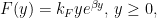
First we’ll use the following plot to place Mr. Stokes’ post in context.

Lord Monckton views the climate system’s equilibrium temperature 


Observational studies like Lindzen & Choi 2011 have led many of us to believe that ECS is actually much lower than that—if there really is such a thing as ECS. In a video that introduced his theory as a “mathematical proof” that ECS is low, though, Lord Monckton said of previous ECS-value arguments that they had “largely been a competition between conjectures.” He may agree with researchers like Lindzen & Choi, he said, but “they can’t absolutely prove that they’re right.” In contrast, “we think that what we’ve done here is to absolutely prove that we are right.”
By in essence projecting those points to the no-feedback, 
“Once that point—which is well established in control theory but has, as far as we can discover, hitherto entirely escaped the attention of climatology—is conceded, as it must be, then it follows that equilibrium sensitivity to doubled CO2 must be low.”
In the passage quoted above, Mr. Stokes’ post contested that theory. So we’ve added a hypothetical 
3. “Underlying Mathematics”
In a reply to Mr. Stokes’ post Lord Monckton diagrammed his version 
However, by treating the (counterfactual) no-feedback temperature
For this purpose we’ll simply adopt the more-general notation that the system produces a response 

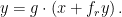
That is, the output temperature 


This is all seemingly simple. But even seemingly simple equations can be hard to interpret. Moreover, Lord Monckton’s theory requires that we deal with entire quantities rather than just small perturbations, so we can no longer ignore nonlinearities.
Therefore, since the formulation 


To map this forcing-input formulation to Lord Monckton’s temperature-input formulation 


4. Example-System Functions
Now we reach specifics: we’ll define the functions 

In doing so we won’t attempt to match the actual climate relationship between equilibrium temperature and forcing. For one thing, no one really knows what that relationship is throughout the entire domain that Lord Monckton would have us acknowledge. To the extent that an equilibrium relationship does exist, moreover, temperature almost certainly isn’t a single-valued function unless that function’s argument is a vector of forcing components instead of the scalar total thereof we’re assuming here. (Those complications are among the reasons why focusing on perturbations is preferable.)
But the question that Lord Monckton’s purported mathematical proof raises isn’t whether we know the relationship; it’s whether, without knowing what that relationship is, high ECS values can be ruled out mathematically. So we’ll merely choose simple relationships that exhibit a high ECS value and watch for any contradictions of what Lord Monckton called “the mathematics of feedback in all dynamical systems, including the climate.”
4.1 Open-Loop Function
For our open-loop function

Note that with 


As we see, 

Since 

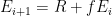
Note also that we refer to both quantities as “open-loop gain”: each is a gain that the system would exhibit if there were no feedback to “close the loop.” Perhaps confusingly—but I think logically—the discussion below uses similar expressions to refer to different quantities.
Specifically, closed-loop gain will refer to the gain that results when feedback does indeed “close the loop.” Lord Monckton sometimes calls this the “system-gain factor.” And just plain loop gain will be the internal gain encountered in traversing the loop: what Lord Monckton occasionally calls the “feedback fraction.” The loop gain results from combining the open-loop gain with the feedback ratio, which we will presently introduce in connection with the feedback function.
Again, the quantity to which our open-loop function 

4.2 Feedback Function
Climatologists sometimes get media attention by speaking of a “tipping point.” But the particular feedback function we chose for the Fig. 1 curve wouldn’t cause one. Since the behavior it results in thereby lacks one of feedback’s more-interesting features, we’ll instead adopt the following feedback function, which causes a tipping point not far beyond the doubled-CO2 equilibrium temperature:
where 


Note that in our feedback-function choice we differ with Lord Monckton’s critics who object that feedback can only be a response to perturbations. Like the Fig. 1 curve’s feedback function, our example, tipping-point-causing function is responsive to the entire output. To be sure, the response seems to become significant in both cases only as the temperature approaches ice’s 273 K melting point; the response approaches zero as the output temperature does. But actually working through the resultant example-system behavior near absolute zero reveals that because of the high forward gain we saw in Fig. 3 the feedback is great enough to cause instability.
Furthermore, although the example function’s value at the doubled-CO~2~ temperature approximates that of the feedback function responsible for Fig. 1, it exceeds it at temperatures very much above or below that temperature. In particular, our chosen function’s feedback to the emission temperature will be even greater than the Fig. 1 function’s.
Now, I don’t really think either of those feedback functions is like the actual climate’s feedback function. I personally don’t think the actual climate has much net-positive feedback at all.
But that’s not the point. Lord Monckton claims to have developed a mathematical proof. That means showing that accepting a high ECS value for the sake of argument would lead to a contradiction with “the mathematics of feedback in all dynamical systems, including the climate.” So the point isn’t whether we believe that premise. It’s whether accepting the premise leads us to a contradiction. And we will search in vain for contradictions among the implications of a system’s exhibiting not only a high ECS value but also a tipping point.

The plot above shows the resultant feedback ratio, i.e., the quantity that multiplies the output or increment thereof to yield our feedback function’s corresponding feedback quantity. It’s the feedback function’s average (large-signal) slope 


Different feedback-ratio functions, plotted above, result if we instead take Lord Monckton’s temperature-input view of the system. Those functions are average and local slopes of a different feedback function, of the function 

The different views’ feedback ratios are somewhat similar at the higher temperatures we’re interested in, but their low-temperature behaviors are quite different. That doesn’t mean that the temperature-input view is wrong. In fact, although I believe the forcing-input view is usually preferable, the temperature-input view may be the more-informative in the case of feedback ratio, which in the temperature-input view happens to equal that view’s loop gain (Lord Monckton’s “feedback fraction”).
5. Resultant Behavior
5.1 Closed-Loop Function
Having now defined our system’s open-loop and feedback functions, we turn to the resulting closed-loop function, i.e., to the function 


This plot illustrates the tipping point we so chose our feedback function as to cause. No (equilibrium) output values correspond to input values that exceed about 273 W/m2. That’s because any higher input value would cause the output to increase without limit: the system would never reach equilibrium. (If pressed, tipping-point partisans would presumably admit to some limit, but let’s just assume their limits are off the chart.) As we will see in due course, inputs that exceed the tipping-point input correspond to a small-signal loop gain that necessarily exceeds unity.
Although the output increases without limit for those values, Lord Monckton says instead that a (large-signal) “feedback fraction” 


Unlike the input, the output has equilibrium values that exceed its tipping-point value, which for the output is about 301 K. The curve’s dotted portion represents them. The dots indicate that the corresponding states are unstable.
You can get an idea of what unstable means by supposing that negative temperatures have meaning in Lord Monckton’s linear 
The example system will similarly tend to flee the unstable states and possibly blow up. The example system is nonlinear, though, and the direction of the nudge determines whether it actually does blow up or instead falls to a stable value, i.e., from the dotted curve to the solid one.
Having seen the output behavior from the forcing-input view, let’s turn to Lord Monckton’s temperature-input view. That is, let’s consider the function 


This view suppresses the nonlinearity in the relationship between forcing and temperature. Since the input is simply what the output would have been without feedback—whose ratio to output is very low throughout most of the function’s illustrated domain—the output over much of the curve nearly equals the input. Toward the right, though, the output pulls away. And, just as in the previous plot, there’s a tipping point.
5.2 “Feedback Fraction”
Now we come to what is perhaps the most-consequential quantity: the loop gain, or, in Lord Monckton’s terminology, the “feedback fraction.” Here again we will see the importance of distinguishing between large- and small-signal versions.

The plot above confirms what we may have surmised from the previous plot: the loop gain is near zero over most of the function domain. But above-unity loop gains on the plot’s right impose the limit we observed on equilibrium-state input values.
Note in particular that it’s the small-signal version of the loop gain whose unity value imposes the limit; the large-signal loop gain is quite modest right up to the tipping point. So it’s important to keep track of which quantity Lord Monckton intends when he discusses the “feedback fraction.”
(Obscure technical note for feedback-theory types: Because of the high small-signal open-loop gain near absolute zero, the system is unstable in that neighborhood even though the feedback
Recall that loop gain is the gain encountered in traversing the loop. For the forcing view the large-signal loop-gain version is therefore the ratio 

Since a unity value of this dimensionless quantity’s small-scale version represents the stability limit, one might think it would be the same thing in both views. If we actually work it out, though, we see there’s a difference.
For the temperature-input view the large-signal loop-gain quantity is the ratio that the feedback temperature 


But a comparison of the two views’ small-signal loop gains is instructive:

Although their small-signal tipping-point values are the same in both views, the different views’ loop gains otherwise differ.
5.3 “System-Gain Factor”
We finally come to closed-loop gain. This time we’ll start with Lord Monckton’s temperature-input view. In that view the large-signal version is 


But by definition the quantity whose multiplication by 


Now, in actuality his approach probably would not result in a serious underestimate if, as many of us believe, ECS is low. That’s because a low value would not result in the great between-version difference that the plot depicts. But that fact doesn’t support Lord Monckton’s theory.
The problem is that his theory’s targets aren’t people who already believe ECS is low. He characterized his theory as a “way to compel the assent” of those who would otherwise believe ECS is high. It would compel assent, he said, because, unlike previous ECS arguments, his theory isn’t a mere conjecture; it’s a proof.
But a proof of low ECS can’t be based on assuming low ECS to begin with; that would be begging the question. Nor would the assent of someone who thinks ECS is high be compelled by an approach that greatly underestimates ECS when it is high. What could arguably compel assent is for the high-ECS assumption to result in contradictions of “the mathematics of feedback in all dynamical systems, including the climate.” That’s why we took a high-ECS system as our example: to expose any such contradictions. But we found none.
Now a point of clarification about the plot. The dotted curves mostly represent unstable equilibrium states as they did in previous plots. But here there’s an exception: the dotted black curve’s vertical segment on the right, at the maximum equilibrium-input value. That segment is merely the line between positive- and negative-infinity values: its abscissa is the value at which the closed-loop gain switches abruptly from positive to negative infinity. So no equilibrium states actually occur on that vertical segment.
It might therefore have been less distracting to omit that segment from the plot. But it provides another opportunity to point out how hard it can be to interpret even simple algebraic equations properly. The corresponding discontinuity in the hyperbola of linear-system gain ratio as a function of loop gain is the basis of Lord Monckton’s above-mentioned belief that loop gains greater than unity imply cooling:

That interpretation is wrong, of course; Fig. 8 showed us that equilibrium output temperature continues to increase beyond the transition to instability.
In the electronic-circuit context Lord Monckton has analogously interpreted that discontinuity is as being the point “where the voltage transits from the positive to the negative rail.” That interpretation is beguiling because of the audience’s experience with audio-system feedback. After all, unity loop gain is the basis for squeal when sound systems suffer from excessive feedback, and that oscillation certainly involves a lot of voltage “transiting.”
One problem with such interpretations is that the hyperbola is valid only for constant open-loop gain. More important, they ignore that the relationship represented by the hyperbola is an equilibrium relationship: the hyperbola doesn’t apply to dynamic effects like oscillation. (Well, the equation on which the hyperbola is based actually can be used to characterize steady-state oscillation. But that would require complex values: the geometric representation would require four dimensions instead of the hyperbola’s two.)
So attempts like Mr. Stokes’ to demystify the feedback equation itself are all well and good. But it’s also important to recognize that the equation’s very simplicity can be misleading, even for someone who “was given training in the mathematics of what are called conic sections.”
Now let’s complete our study of the system’s behavior with the other view of closed-loop gain.

Instead of slightly increasing as the temperature-input view’s large-signal gain did, the forcing-input view’s actually continues to decline right up to the tipping point. But the overall effect is the same: the small-signal gain rises dramatically as the tipping point is approached, whereas the large-signal gain does not.
In short, we’ve worked through a counterexample to the proposition that high ECS values are inconsistent with a system whose feedback responds to emission temperature. In doing so we’ve detected no contradictions of feedback mathematics. But by juxtaposing small- and large-signal versions we’ve seen how important it is to distinguish between them consistently.
6. “Near-Invariant”
Before we conclude, we’ll use one of Lord Monckton’s reactions to such counterexamples to illustrate why it’s important to “work it out” and not just “scope it out.”
Ordinarily Lord Monckton’s reaction to such counterexamples is merely to express his disbelief that the function could be so nonlinear. Or he makes the physical argument that the quasi-exponential response of evaporation to temperature somehow conspires with the quasi-logarithmic response of forcing to concentration to make the entire sum of water-vapor, albedo, lapse-rate, cloud, and other feedbacks linear. Again, though, such arguments are irrelevant. The point isn’t whether we think the function is nearly linear. It’s whether that’s what feedback math requires: it’s whether Lord Monckton has as he claimed achieved an actual proof rather than a mere conjecture.
But this time he argued as follows that it’s “official climatology,” not feedback theory, that imposes the near-linearity requirement. (Presumably he meant “near-invariant” instead of “near-linear” in writing that “official climatology’s view” is “that the climate-sensitivity parameter . . . is ‘a typically near-linear parameter’.”)
“[The counterexample is] spectacularly contrary not only to all that we know of feedbacks in the climate but also to official climatology’s view that the climate-sensitivity parameter, which embodies the entire action of feedback on temperature, is ‘a typically near-linear parameter’.”
“It is only if one assumes that there is no feedback response to emission temperature that climatology’s system-gain factor gives a near-linear feedback response. . . .
“It is only when one realizes that feedbacks in fact respond to the entire reference temperature and that, therefore, even in the absence of the naturally-occurring greenhouse gases the 255 K emission temperature itself induced a feedback that it becomes possible to realize that, though official climatology thinks it is treating feedback response as approximately linear it is in fact treating it – inadvertently – as so wildly nonlinear as to give rise to a readily-demonstrable contradiction whenever one assumes that any point on its interval of equilibrium sensitivities is correct.”
(As an aside we note that Lord Monckton left unspecified the standard by which a system like that of Fig. 1 can be said to be “wildly nonlinear”. Nor did he “readily [demonstrate]” a contradiction that would arise even from a sytem like that of Fig. 8, which we so designed as to provide an imminent tipping point.)
For the sake of convenience we’ll use Lord Monckton’s notation to unpack a couple of those assertions.
First, although he often criticizes “official climatology” for focusing on perturbations in its ECS calculations, he apparently chose in this context not to interpret climatology’s use of “near-invariant” or “near-linear” as limited to the ECS calculation’s perturbation range; he interprets the near-linearity as applying to the
Second, the projection line in Fig. 1 above illustrates what he seems to mean by “It is only if one assumes that there is no feedback response to emission temperature that climatology’s system-gain factor gives a near-linear feedback response.” If you’re considering the stimulus to be only the portion of
That his interpretation of “official climatology’s view” thus results in a contradiction isn’t a very compelling argument by itself. His interpretation is almost certainly a misreading of the literature. And, if you choose a contradictory interpretation over the more-probable non-contradictory one, you’re bound to find, well, a contradiction.
But in a further comment he seems to say that climate-model results confirm his interpretation of “official climatology’s view”:
“[W]e are not doing calculations in vacuo. The head posting demonstrates that official climatology regards—and treats—the climate-sensitivity parameter as near-invariant: calculations done on the basis of its error show that the system-gain factor in 1850 was 3.25 and the mean system-gain factor in response to doubled CO2 compared with today, as imagined by the CMIP5 ensemble (Andrews+ 2012), is 3.2. Looks pretty darn near-linear to me.”
Climatology must have intended a nearly linear function, that is, if its slope exhibits so little variation in that interval. And, if climatology intended it to be nearly linear, then feedback would reach zero at the emission temperature: climatology’s position is that there’s no feedback to the emission temperature.
Before we show that this standard for “pretty darn near-linear” is too loose to rule out every counterexample, let’s recognize that drawing an inference from differences so dependent on ensemble selection is a parlous undertaking. For instance, a polynomial fit to the combination of those “system-gain factors” with the 

But let’s nonetheless assume “official climatology’s view” to be that the closed-loop gain won’t vary by more than 3.25 – 3.20 = 0.05. As the plot below shows, this assumption still doesn’t support the inference that “official climatology” has “made the grave error of not realizing that emission temperature 

For the interval over which Lord Monckton reports the variation in “system-gain factor” the plot displays the temperature-input view’s closed-loop-gain functions not only from the example system but also from that of Fig. 1. As to the large-signal versions, the different feedback functions’ results are virtually indistinguishable, and they vary only negligibly over the interval.
As to the small-signal versions, it’s true that the variation caused by the example, tipping-point-causing feedback function greatly exceeds the arbitrary “near-linear” limit, 0.05. But that limit, which made the “official climatology” closed-loop function
Although a closed-loop function may look “pretty darn near-linear” when we just scope it out, that is, it can look quite a bit different when we actually work it out.
7. Conclusion
The equilibrium scalar feedback equation is the most rudimentary of feedback topics; the algebra is trivial. Yet, as we saw in connection with Fig. 12’s hyperbola, its interpretation isn’t straightforward even when the system is linear. And for nonlinear systems it provides a good occasion to recall that simple rules can result in complex behaviors. So any feedback question calls for following that professor’s advice: Don’t just scope it out; work it out.
We’ve already crossed the tipping point about 11,000 years ago, after the Younger-Dryas was soundly rejected by continued insolation forcing of the incipient Holocene. Now it is just a mainly a linear descent back to the norm for the Pleistocene in which we live. CO2 is our friend. Some day science will recognize that, and the today’s idiots who call it ‘carbon pollution’ will be looked at in the history books in disdain.
I was fascinated to find that fields of wheat were found to stop growing in still air as they had insufficient CO2 (having sucked it all out of the vicinity) even though they had plenty of water, sunlight and soil. In the 50s…
Intriguing comment but utterly valueless in the absence of a link or reference. Do some crops prosper in windy areas?
I had a link to a UK textbook that described that exact condition. In the UK, when levels were closer to 300 ppm, wheat crops stopped growing in the afternoon of high growing days. The local levels of CO2 had dropped too much for photosynthesis to continue. The air mixed sufficiently overnight to restore the levels, plus the plants themselves, begin respiration and emit CO2..
The textbook has been updated, and that paragraph removed. I will take the high road and assume it has been removed because the now higher levels of CO2 allow the plants to grow the entire day.
Regardless, I can support what Chas said, even if the references have been removed from the web. You can believe it or not; matters little to me.
I can add that Dr AD Karve of ARDRI, Pune, India, has demonstrated the opposite effect using five ft high plastic curtains to divide fields into a grid of small “rooms”. At night, on windless nights, the CO2 aspirated by plants and the ground is held in the “rooms” because of its density, and is available in the morning to enhance growth. The plastic curtains prevent it wafting away. For a given wind, there is a given wall height for a given % retention.
In the absence of daytime wind, the “room” will run out of CO2. However some places there are windy days and windless nights for a net gain.
A similar result was found with corn. CO2 monitors in the fields found that on windless days the levels fell off the scale of the instruments.
That is my best guess for the probable reason for the finding that corn, despite being a C4 crop, benefits considerably from elevated CO2:
https://www.tandfonline.com/doi/abs/10.1080/00103624.2018.1448413
Modern corn cultivars are so fast-growing and productive that a cornfield can quickly use up all the available CO2. A higher starting level in the morning means that, on a windless day, the corn can grow until later in the afternoon, before running out of CO2.
I shall be giving a talk at the Heartland conference next week, in which all will be made clear. All that need be said at this stage is that feedback processes necessarily respond to the entire reference temperature present at any given moment; and that in that fact lies the key to constraining equilibrium sensitivities. Readers will, of course, decide for themselves whether it is more likely that our tenured professor of control theory has gotten control theory right than that a retired lawyer has gotten control theory right. My money is on the tenured professor.
And how pray tell are negative feedbacks addressed? Rising temperature presumably increases humidity by the Clausius-Clapeyron-Koutsoyiannis equation – But that increases the probability of clouds, greater shading, and increased albedo providing negative feedback – per Willis Eschenbach’s nature’s thermostat explorations.
See Koutsoyiannis, D., 2012. Clausius–Clapeyron equation and saturation vapour pressure: simple theory reconciled with practice. European Journal of physics, 33(2), p.295. (equation 42)
http://www.itia.ntua.gr/getfile/1184/2/documents/2011ejp-clausiusclapeyron-pp.pdf
“Readers will, of course, decide for themselves whether it is more likely that our tenured professor of control theory..”
I think this line of argument that crops up at WUWT from time to time is funny. It goes
“We have found that all those scientists for the last century have been making a grave error!
You make find our argument a little incoherent, but you have to believe it.
X, my co-author, says so, and he is a tenured professor!”
‘Some day science will recognize that, and the today’s idiots who call it ‘carbon pollution’ will be looked at in the history books in disdain.’
First we have to survive past these same idiots. That’s still up in the air at the moment.
Over 3 1/2 billion years and no ‘tipping point’ has ever happened. That’s a well tested system.
what do you call an ice age? And best guesses of past climates suggest that there was at
least one snowball earth in the past where nearly all of the earth was cover in ice. The
creation of a snowball earth climate is definitely a tipping point. Other tipping points
are the beginnings of photosynthesis leading to large amounts of oxygen in the atmosphere.
For ‘runaway’ globull warming. Zharkova et al worry me about a possible ice age. I see no easy way to mitigate an ice age whereas warmth suits us hairless apes…..
You aren’t making sense a tipping point is a condition you never get out of. If we passed a tipping point into a snowball earth we would still be there. You may be thinking of a metastability or cascading point hard to work out what exactly you are trying to say.
Welcome to the simulation.
LdB,
A tipping point represents a sudden shift from one meta-stable state to another.
There is nothing that says that it is irreversible just that the shift happens much
faster than the usual change. The issue is that “tipping point” is not a scientifically
defined term and people can use it to mean anything they want.
The issue is that “tipping point” is not a scientifically defined term and people can use it to mean anything they want.
Including you, it would seem . . .
As comments have said says that is your definition not something others are going to understand.
+10!
The earth recovered from each “ice age” and the alleged snowball earth.
A few million years ago, the CO2 levels were over 5000ppm, and no tipping point was hit.
What makes you think we are going to hit one at 500ppm?
Large scale signal responses are step functions. These would be events such as an Astroid impact or volcano. Everything else is small signal (glaciation cycles for example). If you have a step function that dampens out over time, you must by definition have a critically or over damped system, otherwise you oscillate (from which you never recover). You can estimate the sensitivity (gain of the system and phase margin) from the time it takes to ring out a perterbation.
If there ever WAS a climate tipping point:
https://www.google.com/search?client=ms-android-huawei&ei=M00xXd6tEYLLrgS8xbW4Ag&q=tipping+point+climate&oq=tipping+point+&gs_l=mobile-gws-wiz-serp.
Joe, this paper is in DESPERATE need of an abstract. Just what is it that you are setting out to show, how did you show it, what did it mean, what does it say about Monckton’s claims, if his claims are wrong where are they wrong? That kind of thing.
Without that I’m finding it nearly impossible to follow your argument.
Heck, I had a hard time getting past the labels in Figure 1, where both a vertical and horizontal line are labeled “Emission Temperature”, and the heavy black line is never identified …
Please take this in the sense intended, which is to make your study understandable to the greatest number of people … including me …
Best regards,
w.
Well, it was titled “Remystifying…” 🙂
Well I was going to post saying he had succeeded !
My attention span was getting strained about 1/3 of the way through and reached a tipping point after the mid-point.
The take home point seems to be that if you want to use the whole signal, feedbacks are non linear and all the nice, easy linear maths goes out of the window. At that point, climatologists and climate modellers throw up their hands in despair and go to look for a real job.
Until we understand cloud formation to a point where we can firstly MEASURE it to high accuracy then model it and get results which match observations, the rest of the game is a total waste of time and is just sand being thrown in our eyes to blind us to what the real aims of the alarmists are.
Agenda 21 is probably the most succinct description.
Monckton’s would-be paper is a side show, though I do think that like anything, it should get due process and either be published for discussion or rejected with a valid and thorough reason. “Because I don’t like” does not count.
That this blatant gatekeeping is still going on over ten years after Climategate is reason enough to shut down funding of climate research altogether until they start to play by the rules of science.
Greg Goodman,
Bravo! You summed this post up well.
Agreed!
Well noted. Perhaps Moderators can make sure there is an abstract like that at top of every article. Just basic writing.
Your comment is spot on. However IMHO this is a common problem with many articles on WUWT. As an “educated layman” (I’m an engineer) I often have great difficulty piecing together the context and structure of the claims made in articles here. I think articles longer than a few paragraphs should be required to have an abstract. In my own experience writing an abstract up front helps streamlining an article or report tremendously.
Aye that;-)
As Lord Monckton told you, his “main point . . . is that such feedbacks as may subsist in a dynamical system at any given moment must perforce respond to the entire reference signal then obtaining, and not merely to some arbitrarily-selected fraction thereof.”
Lord Monckton left a yawning chasm between that point, which I’ve called his “entire-signal rule,” and the conclusion that he says follows from it: that “equilibrium sensitivity to doubled CO2 must be low.” That logical gap has often been obscured by Lord Monckton’s failing adequately to distinguish between large- and small-signal versions of, e.g., his “system-gain factor.” The head post shines light on that gap by exploring the difference between same-named quantities’ large- and small-signal versions. The head post also demonstrates some fundamental feedback misconceptions under which Lord Monckton seems to be laboring.
Let me remind you that this whole thing started in the video I referenced above, where Lord Monckton drew a distinction between mere conjectures and absolute proofs. Now, I personally think it’s quite likely that ECS is low, as Lord Monckton contends. Since I do, and since that would mean the (small-signal) ratio it bears to the value it would have without feedback is also low, I also think it’s plausible that this small-signal ratio is approximated under current conditions, as he says it is, by what he calls the “system-gain factor,” which is the (large-signal) ratio that the (entire) equilibrium temperature E bears to the (entire) value R it would have without feedback; that large-signal ratio is relatively small, too.
But that’s all just a conjecture; as he said of work such as that by Lindzen & Choi, it does not absolutely prove ECS is low.
In contrast, he said, “we think that what we’ve done here is to absolutely prove that we are right.” Specifically, he said, “I can . . . prove that the form of the equation [climatology’s ] is erroneous and leads to a large exaggeration.”
His “proof” was that “the mathematics of feedback in all dynamical systems, including the climate, comes from electronic circuitry” and that the input and output
  in the feedback equation relationship
  from Hendrik Bode’s Network Analysis and Feedback Amplifier Design “are absolute values: they are not deltas, they are not changes. . . .”
He gave no real reason why those equations couldn’t both be true simultaneously. But he called attention to the fact that climatology’s value for what he currently calls the “feedback fraction
  ” is several times the climate equivalent of Dr. Bode’s corresponding quantity
  .
.
What the head post does, among other things, is show that such a difference shouldn’t be surprising; although both quantities are what I’ve called “loop gain,” the former is its small-signal version, whereas the latter is its large-signal version.
A significant difference between large- and small-signal versions is contradictory only under the assumption that “all dynamical systems” that have feedback are nearly linear, as the vacuum-tube operating regions were in the telephone-system repeaters that gave rise to the lectures Dr. Bode’s text was based on. With repeater design as those lectures’ background, it was convenient for Dr. Bode to assume linearity in his text’s initial mathematical development. But in that technological milieu the lectures’ audience would have known without being told that reducing the remaining nonlinearity was feedback design’s entire raison d’être. Even in electronic circuits, moreover, near-linearity is hardly universal. Much less is it a given that “all dynamical systems” in which feedback operates are nearly linear.
But Lord Monckton argues as if his entire-signal rule were tantamount to a feedback-math requirement that E(R) be nearly linear, like those repeaters’ vacuum-tube operating points. Aside from personal attacks on me, most of his replies when people point out the climate system’s possible nonlinearity fall into three categories. (1) Expressions of disbelief that E(R) could be nonlinear enough to exhibit a high ECS value while providing a feedback response to the emission temperature. (2) Arguments that such nonlinearity would be inconsistent with the near-linearity in E(R) that he thinks references by “official climatology” to near invariance requires. (3) Arguments that the quasi-exponential response of evaporation to temperature somehow conspires with the quasi-logarithmic response of forcing to concentration to make the entire sum of water-vapor, albedo, lapse-rate, cloud, and other feedbacks linear.
As to (1), the high-ECS curve in Fig. 1 above shows that “near-linearity” is a question of degree that he’s failed to establish by a formal mathematical proof. As to (2) the section called “Near-Invariant” observes that his argument is based on a tortured interpretation of the literature; a more-likely interpretation is the “official climatology” does indeed imply that level of nonlinearity. And it shows that what he thinks is quantitative support for that argument is not. Finally, (3) is no less a conjecture than he says work by researchers like Lindzen & Choi is, so it, too, falls short of the absolute proof he claims he’s achieved.
Incidentally, at 35:20 into that video Lord Monckton says he and his team started out with a tricked-out version of Fig. 12 above, which made them realize of “official climatology” that “they hadn’t a clue what they were doing.” He explained, “I knew about this curve . . . . I recognized it at once because I’m a classical architect by training, and I was given training in the mathematics of what are called the conic sections.” In the course of its discussion the head post explains that in feedback mathematics this hyperbola he’s fond of referring to doesn’t mean what he says it means.
I apologize for being obscure. I made an extensive study of control-systems theory and attendant feedback mathematics a half century ago and for my sins have been required to return to it in some depth numerous times since. As a consequence I don’t always take into account that we aren’t born knowing this stuff.
Why would you even bother with this junk it’s a 1D stupidly simple model which even by climate science standards is naft.
Apparently it’s so simple that John Tyndall worked it all out in 1859 or so some people say.
Because Lord Monckton has used it and may crowd-fund a lawsuit based on it. So due diligence by readers who may want to support such an effort should include considering its implications.
The law suit is almost certainly justified, even if the paper is flawed. That legal process should be allowed to go ahead without it being short-circuited by someone showing why the paper is flawed and the defendant getting a free pass.
Accountability if far more important to climatology, than the technical accuracy of one paper. Even if CofB is not a boffin on feedbacks he is certainly tenacious and well connected enough to succeed in the legal endevour.
In that he deserved undivided support.
. . . may crowd-fund a lawsuit based on it.
Ever the angelic philanthropist with your concern for the wallets of others? Such altruism from the good barrister!
So due diligence by readers who may want to support such an effort should include considering its implications.
Due diligence in considering said implications presupposes digesting a document that can be understood. Understanding such a paper presupposes the writer is capable of rendering an adequate composition.
Have you accomplished the second in order for we ignorant half-wits to manage the first?
A naive application of basic physics gives a non-alarming climate sensitivity. Hansen used feedback analysis to pump up the sensitivity to alarming levels. Currently, and fifty years ago, when you first encountered feedback systems, the reference level is shown explicitly, ie. operational amplifiers are shown with inverting and non-inverting inputs. The analysis used by Hansen was based on vacuum tubes and the reference was implicit, ie. signal ground. If you’re going to use feedback analysis, you have to take the reference into account.
When people insist that the climate feedback system responds only to perturbations, the simplest explanation is that the system has a DC gain of zero. That would mean that ECS would be zero.
Monckton consulted a control systems expert. It’s pretty clear that Hansen didn’t. It’s also clear that the vast majority of climate scientists did not do so.
There is an adage in engineering, “Never put pencil to paper until you know what the answer should be.” In other words, scope it out, then work it out. The problem with applying math to problems that you don’t understand is that it produces garbage results. About 50 years ago a professor complained to me that students would attempt to apply an equation to a problem, no matter how inappropriate. Over my career I learned that the problem isn’t restricted to students.
+10
Would be great if you would boil down what you are trying to say in three or at most four sentences, taking guidance from Willis (above) on what should be included…
Keep in mind LM doesn’t ever describe this as a definitive answer. His main thrust is to take assumptions held by many mainstream climate scientists and prove them false. If his basis for the project is wrong then blame the mainstream scientists who continue to use traditional feedback as a crutch to explain temperature changes.
I don’t believe I’ve held Lord Monckton responsible for any of the “official climatology” data, and I’ve additionally accepted for the sake of argument his own entire-signal rule.
What I contest is his contention that by employing that rule as a premise he has “absolutely proved” that ECS is low.
In my eagerness to get to breakfast I neglected to address Mr. Eschenbach’s Fig. 1 question.
The horizontal and vertical “emission temperature” lines’ intersection represents what Lord Monckton says is “official climatology’s view”: that without greenhouse gases the with- and without-feedback equilibrium temperatures would be the same and would equal the emission temperature’s (current) value. In other words, he says it’s “official climatology’s view” that there would be no feedback at the (current value of the) emission temperature.
The dashed line represents, as the head post puts it, “projecting those [pre-industrial and doubled-CO2] points to the no-feedback, E=R line.” That is, it’s a graphical representation of Lord Monckton’s reasoning, which is that “official climatology” can think the E(R) curve is that steep—and thus that ECS is that high—only if it also thinks, contrary to Lord Monckton’s entire-signal rule, that the emission temperature results in no feedback. His argument is based, in other words, on the fact that a line having that high a slope projects to the emission temperature on the no-feedback line (rather than, as Lord Monckton would have it, having a slope shallow enough to project to the origin).
That’s why Lord Monckton wants to say it’s “official climatology’s view” that feedback is linear, and in particular is proportional to temperature but, in violation of the entire-signal rule, is proportional only to that portion of the temperature that exceeds the emission temperature. Otherwise, “official climatology” could be taking an internally consistent view, such as the one that the curve illustrates: that some feedback, such as a result of albedo change, could occur even at the (current value of the) emission temperature. If he insists on its being “official climatology’s view” that linearity of feedback as a function of only the temperature portion that exceeds the emission temperature, then he can find a contradiction between high ECS and Lord Monckton’s entire-signal rule.
If by “heavy black line” Mr. Eschenbach means Fig. 1’s nonlinear curve, then the heavy black line is the “hypothetical E(R) curve” that “[illustrates] what high-ECS proponents might think.” By passing to the left of the two emission-temperature lines’ intersection point, Fig. 1’s curve illustrates that it wouldn’t be logically inconsistent for “official climatology” to believe both (1) that there’s some feedback to the (current value of) emission temperature and (2) that ECS is high, as the curve’s slope between the pre-industrial and doubled-CO2 points indicates.
As literature statements such as the one about further albedo enhancement in Lacis et al. 2010 indicate, that curve is in fact more likely than Lord Monckton’s exegesis to be representative of “official climatology’s view.”
Again I apologize for being obscure. Fig. 1 replaced four figures in the first draft, which set Lord Monckton’s thinking out in more detail. But (1) my experience suggested that so direct a criticism of Lord Monckton’s theory would probably have led to the post’s being spiked, and (2) those figures’ exposition seemed mind-numbingly obvious to someone who has succumbed to morbid fascination at the popularity of Lord Monckton’s theory. So (a relic of my misspent youth in honor of Lord Monckton’s penchant for Latin:) brevis esse laboravi, obscurus factus sum.
Yes, feedback analysis can be confusing and counter intuitive which is why amateurs like Hansen and Schlesinger misapplied it so thoroughly and why so many alarmists like Nick are so confused.
The bottom line is that the surface emits 1.62 W/m^2 per W/m^2 of solar forcing and if you want to think of something as being feedback like, it’s the power replacing the 620 mw per W/m^2 of surface emissions per W/m^2 of forcing above and beyond an ideal BB which emits exactly 1 W/m^2 per W/m^2 of forcing.
Only feedback expressed in W/m^2 can be added to forcing also in W/m^2 and when 1 W/m^2 of forcing is added to 620 mw of feedback and then amplified by the assumed unit open loop gain, the output is 1.62 W/m^2 of surface emissions. Since all W/m^2 of solar forcing from the Sun arrive at the same time and are indistinguishable from each other, all W/m^2 of solar forcing must have the same feedback and gain applied to them. Note that increasing CO2 is not forcing but can be considered equivalent to some amount of forcing keeping CO2 concentrations constant. Only the Sun is the forcing since without a Sun, GHG’s have no effect, equivalent forcing or otherwise!
BTW, the assumption of unit open loop gain is obfuscated by the non linearity between forcing and an output improperly considered to be temperature, where the proper output would be the equivalent W/m^2 of surface emissions corresponding to a temperature.
The error that led to the implicit assumption of unit open loop gain was Schlesinger’s conflation of the feedback factor with the feedback fraction which are only the same when the open loop gain is 1. The feedback factor is an arcane quantity given as the feedback fraction times the open loop gain. This become an obsolete metric since in modern amplifiers, the open loop gain is often considered to be infinite, thus the feedback factor is also infinite while the feedback fraction is limited to be between -1 and 1. Schlesinger fudged a fake non unit open loop gain as a linear scaling factor that converts W/m^2 into a temperature but that definitely does not amplify W/m^2 into a temperature.
Thanks, Willis.
Mystification is one of the methods used in propaganda. You have an unsubstantiated assertion. You repeat it Ad Nauseam. Then you appeal to authority. Science, you know. If someone is still questioning you, you give a reference that is impossible to comprehend. Like climate models. To be sure you use a paywall and hide the code and measurement data,
Wring a paper over and over again is a good practice. Say it so that readers can follow. If you can’t, maybe you did not understand it yourself.
Mystification via smoking mathematical mirrors?
If there is positive H2O feedback from the CO2 warming, they you must also take the negative feedbacks into account. Eg. the extra H2O comes from evaporation from the oceans mostly, and since evaporation is endothermic, it cools the surrounding area (thus a negative feedback). That water vapor then forms clouds which are also a negative feedback (mostly).
ggm:
Yes you have raised a vital point here, with water being the joker in the pack.
Water is only a GHG in the absence of phase change; producing a positive feedback. At phase change, however, the absorbed energy is converted to Latent Heat rather than into increased temperature, thus rendering the coefficient “K” in the Planck Equation dF = K*dT close to Zero; which reduces the global Climate Sensitivity IF taken into account. (repeat IF).
At this phase change water becomes strongly negative as feedback; so the net feedback varies with changes in the vapor/liquid ratio prevailing at the time.
A further problem for the modellers is that an increase in energy input whether by the GHG Effect or otherwise results in an increase in evaporation rate rather than an increase in temperature under constant pressure. ( This well known in steam generating plants). This means that, in the presence of water, the global Sensitivity (K) varies with the energy input.
Thus, from the above, applying a constant Sensitivity to the Climate for the purposes of future prediction is not valid.
My regards,
Alasdair
Positive feedback systems are inherently unstable and tend to avalanche uncontrollably. The most common example of this is an audio amplifier – bring the microphone too close to the speaker and you get the characteristic feedback “howl” – this in spite of the fact that all amplifiers have negative feedback to limit this. I once accidentally built positive feedback into an audio amplifier – it would do nothing but howl.
An audio amplifier can amplify by many multiples as long as it is “open loop” – example: If you and your microphone stand miles away from the speakers you can amplify as much as you like – but the moment the amplified sound goes directly back into the microphone – at values higher than the original sound into the microphone – then the feedback avalanches. An audio amplifier is not the best example as it has phase shifting and negative feedback to suppress feedback avalanche howl.
An example of an open loop amplifier is the amplification of a radio signal – the amplification does not amplify the signal in the atmosphere – under these circumstances the Bode amplification factor can run to 50 to 1000 times amplification – but tend to instability at the higher end.
Our climate is a closed system – whatever feedbacks there are act directly on in. To put that in plain simple English, what the alarmists are claiming is that “heat in the atmosphere causes even more heat in the atmosphere etc. etc. etc.”
There is a further problem with using the Bode amplification model – the IPCC only applies it to the peturbations and not the entire reference signal (as pointed out by Lord Monkton).
Now that is in fact how a Bode amplifier works in electrical circuits – a capacitor is used to filter out the peturbations (the alternating current is stripped from the underlying direct current voltage by feeding it through a capacitor “filter”)
Ah-Ha you say, the IPCC approach is correct ! Well for that to be so there has to be some sort of magical filter in the atmosphere that somehow filters out only those changes in temperature and “feed” them selectively to the CO2 “amplifier” – complete balderdash.
Again returning to our electrical amplifier analogue – if you remove the filter capacitor the entire amplifier will go FFFFIZZZZTTTT and blows a fuse as it immediately avalanches if the entire reference signal (voltage) is fed back. (That’s what happens to a radio signal amplifier when the positive feedback capacitor fails short-circuit – restoring old valve amplifiers is a hobby of mine and I’ve seen a few examples of this.)
There is no evidence to suggest that our atmosphere behaves like an electrical amplifier so the application of this formula is at best wishfully grasping at unrelated physics for some legitimacy and is at best only useful as a proximal in the lower range of values for f.
To base extremely expensive policy on such shoddy science is dangerous.
If our atmosphere generated more heat from heat it would explode or near instantly avalanche to the maximum power available.
Even small positive feedbacks tend to avalanche and any feedback greater than 1 in a closed system must absolutely do so – yet the IPCC have a feedback figure of 0.61 ±0.44 – for 99% confidence limits which is impossible (the models work with values up and down from this and this process produces a very strong hyperbolic upward bias).
They do this by hiding it within a climate sensitivity calculation to make it less obvious – but this is clearly designed to cloak an impossibility and provide a hyperbolic upward bias to their modelling. The fact that this is as plain as the nose on your face to anyone who understands thermodynamics and mathematics can only mean that it is a deliberate contrivance.
Some argue that values greater than 1 produce a negative feedback. Mathematically this is false – the equation is clearly bounded by f1 which should be self evident.
As mentioned earlier the Bode feedback equation for electronic amplifiers, which is the very foundation of the IPCC’s alarmism, is – for a closed system – bounded by 1.00 – a boundary conveniently – and contrary to the laws of physics – ignored completely by the IPCC and its alarmist cohorts.
Excreta Tauri Cerebrum Vincit
I don’t see how you can call our climate a closed system? Heat arrives and heat leaves. If we consider the evolution of the system due to increasing CO2 in the atmosphere then that is a whole system change with lags in response due to the likes of time to warm, increases in cloud, changes in albedo and may others. We know for a system with fixed CO2 there are many different ocean oscillations with say 60 year cycles etc. We know that the fluid equations of the atmosphere are chaotic. That’s the canvas on which simple feedback methods are being applied and I don’t buy the validity of such methods in this context.
What we’ve seen on the time since 1880 is a very small rise in temperature compared to historical variations in average temperature ranging by 35 Deg F in the last 1/2 Bn years. And CO2 has lagged temeprature by 800 years
https://en.wikipedia.org/wiki/Geologic_temperature_record#/media/File:All_palaeotemps.svg
And in the graphic we have a sudden 7-8deg F rise shown for the next 80 years, I assume from models.
Too much fantasy
In thermodynamics a closed system is one where the mass of the system never changes. Energy can pass the boundary of the system but mass never enters or leaves.
A sealed cylinder with a movable piston is an example. You can change the temperature of the air in the cylinder by moving the piston in or out. The mass of the system never changes but the temperature of the air will change.
For me this whole exercise of trying to describe the temperature of the Earth using one equation to describe the entire environment is a losing proposition. The environment of the Earth is a multiplicity of thermodynamic open systems where mass and energy are passed among this multiplicity of open systems on a continuous, dynamic basis. Any feedback within each individual open system varies widely as the conditions within the system changes from instant to instant. It’s the very definition of a chaotic overall environment. Trying to define the resulting environment using a simplified “average” equation is bound to fail. It’s the same kind of fallacy used in trying to describe the Earth using an “average” temperature. Not only does the average not tell you if maximum/minimum temps are going up or down it tells you nothing about actual locations on the planet!
As the atmosphere warms it expands, so where is the boundary of the “closed” earth climate system?
“As the atmosphere warms it expands, so where is the boundary of the “closed” earth climate system?”
The “boundary” is between the atmosphere and space. Define them yourself. A boundary is *still* a boundary. Even if space exchanges mass with the atmosphere the atmosphere exchanges mass with space, set the boundary at a point where the impact of the exchanges is beyond simple calculation.
Earth has a defined outer bound wrt energy budget.
The top of the atmosphere.
https://earthobservatory.nasa.gov/images/7373/the-top-of-the-atmosphere
It’s thought of a closed system because matter is not exchanged across its boundaries (close enough for government work).
https://www.windows2universe.org/?page=/earth/climate/what_are_systems.html
But your reference document says the Climate system is open.
“But your reference document says the Climate system is open.”
It does? It says.
“The earth-atmosphere system can be thought of as a closed system. Energy in the form of solar radiation (sunlight) enters the system and eventually exits in the form of terrestrial and atmospheric thermal radiation (heat), while only negligible amounts of matter are exchanged between the earth and space.”
“It is quite intuitive to include the atmosphere as a key component of the climate system, but most experts agree that it also includes the oceans as well as the cryosphere, biosphere, and geosphere. It is important to understand that the system also includes the interactions between the components.”
While the article *does* say: “The climate system is an excellent example of an open system” this is incorrect. The climate is a result of the interactions between the components in the closed system. Climate is not itself a component of the overall system or even a “system” of its own, it is a *result*.
This ^^^^^^^^^
Since Mr. Stokes had already covered it and the post was already too long, I left out what they mean in this context by positive feedback: what in some other circles would instead be considered a reduction in negative feedback.
It all depends on the level of abstraction. See my previous post, in which Fig. 1 is a higher level of abstraction than Fig. 3. Fig. 1 depicts a system as having only positive feedback, but Fig. 3 reveals that there’s negative feedback in what Fig. 1 depicts as the forward block.
So, although actual positive feedback would mean instability in the climate system (but not necessarily in feedback systems generally), what passes for positive feedback in climate discussions doesn’t necessarily mean instability–as the head post’s Fig. 1 system illustrates–because, again, it’s actually just a reduction in negative feedback.
That is the biggest flaw in Monckton’s approach. He lets them have a free pass on the biggest con in the whole game. Pretending that the dominant ( and inconveniently negative ) feedback is not a feedback.
They expend much effort debating whether net f/b is “negative” or “positive” ( which leads to spurious talk of tipping points ) when what they are really discussing is whether it is a bit less negative or a bit more negative. It’s like the “ocean acidification” game, discussing 8.2 to 7.9pH both firmly basic.
Temperature “anomalies” imply any change it not “normal”. Long term average is called “normal” suggesting that any perfectly normal statistical deviation is “abnormal”. All of the natural variability is detrended ( since we “know” what the trend is ) and are all named as the xxx “oscillation”. A term which suggests a net zero cyclic change. They are by definition net zero, because climatologists spuriously and arbitrarily detrend them !
It is all a game of words, not science.
“And, indeed, there are good practical reasons in climate science for treating feedback as something that’s responsive only to changes rather than to entire quantities”
Oh Yes? But outside climate science, we are being led to believe that climate science can predict the future climate with sufficient accuracy to be included in considerations of state policy. But so far, they have not shown sufficient accuracy to be believable.
The problem is simple. The output figure of these climate mathematical models is the sum of all the inputs. Change one of the inputs a bit, and the output changes a bit. So in order to find out the relative weighting of that input, all other inputs must be either known, or held constant. Then, we can do this in turn to have a good model.
Climate science’s problem is that they just don’t know these inputs, or their weighting, and therefore cannot tell. (BTW one of the ironies is that in a model involving feedback, the output is the biggest single input)
I suggest that the author looks again as his Professor’s remark, and see that in order to ‘work it out’, one must have ‘scoped it out’ in the first place.
I think I put your point in a slightly different way when criticising climate models. The models claim to produce ECS as an “emergent” property but they do not. The models have inherent assumptions about ECS and are thus simply calculating ECS based on those assumptions. If the models use first principles, then ECS can be shown and calculated from those first principles without a huge model. But they don’t and so ECS is not emergent but dependent on the assumptions used. As I have said before, these vast models can be condensed to a couple of lines on an Excel spreadsheet in terms of ECS:
Change in CO2
Change in temperature caused by change in CO2
One multiplied by the other.
What we ought to do is to put in what we like for the second line and then run your results through huge models to see what effect increased temperature has on the climate. Run lots of different assumptions and see which one most accurately forecasts what happens. That’s probably the right one. Instead we use the same model to both calculate ECS and use ECS to prove the calculation of ECS. There is an inherent circularity that should be separate because it obscures what the models are actually doing.
I am under no illusion that “official climatology” is anywhere near correct about how much feedback there is. But there is no reason to suppose that its error is what Lord Monckton says.
Specifically, if, as is the case with ECS calculations, all they’re interested in is the change that doubling CO2 concentration will cause if none of the other inputs changes, then perturbations from it are indeed all they need concern themselves with; they (at least think they) know the current state already. The head post depicts taking the entire “signal” into account but still finds that it’s the small-signal quantities–i.e., the perturbation-based ones–that are dispositive.
Joe, all well and good, however, Lord Monckton was only using the IPCC formula, (in his original paper) to demonstrate that believers ignored the complete input signal, using the delta input only.
Yes, there may be flaws on LMs methods, but do you disagree with LMs notion that you can get away with using just the delta and achieve a higher ECS?
I am sure LMs work can be refined and made more complete but he was using the original IPCC values and formula to prove a point.
Steve,
What Monckton did was pull an equation out of the air that he claimed was the IPCC formula.
Nowhere do the IPCC claim that they use his feedback formula for analysing the climate. Rather
they use it to explain the results of the various models. The IPCC use climate models for making
predictions since after all if the climate could be simply modelled using the formula that Monckton
claims they use the climate scientists would not need climate models.
And in any case Monckton uses the feedback formula outside its range of validity and so any results
he gets are meaningless. As many others have stated the feedback formula is nothing but a first order
Taylor series expansion and as such is only valid for small changes in the input forcings.
One objection I had with Lord M’s recent version is that it involved a lot of talk about temperatures down to 0K. And there is some of that here too. Now this is really unphysical; we will never know, or need to know, how the atmosphere behaves when it has frozen. The only range one should be thinking about is from at most about 220K upward, since such temperatures do occur in the upper atmosphere. But these notions are supposed to be whole system models, so even then a temperature of 220K is far too low. But anyway, the point is that a theory that depends on notional behaviour below those levels is off the planet. So I think all the Figs should have been restricted to such a range. In a way it doesn’t matter, because the talk is about what happens if the gradient becomes infinite in a feasible range.
Lord M’s fallacy wasn’t in thinking the functions might be locally linear (citing the IPCC). It was in thinking that they would be linear down to 0K, which could be used to fix the gradient. And then it is very fixed indeed, hence the claimed impossibility of sensitivity. But in fact, as I noted on that thread, if you just assume that E(R) and R converge in the range we know they must, which is down to somewhere where condensing GHG effects disappear, then you get ECS in the IPCC range.
I don’t disagree with your statement that behavior at absolute zero (and fairly far above it) is irrelevant as a practical matter and that no one knows or much cares what it is. But I accepted Lord Monckton’s entire-signal rule for the sake of discussion to illustrate that its implications weren’t what he thought. So showing the entire scale is appropriate.
Also, I profess no great knowledge of the literature. But I think we know from, e.g., Lacis et al. 2010 that whatever degree of linearity “official climatology” agrees on in the CO2-doubling interval isn’t so great as to imply that there’s no feedback at the current emission temperature. So, unless I misunderstand you, I disagree with your contention that “that E(R) and R [must] converge . . . somewhere where condensing GHG effects disappear.”
I think the disagreement is that you think R excludes only feedback from greenhouse gases. But it’s Lord Monckton’s symbol, and he views it as additionally excluding, e.g., albedo feedback. So there’s at least arguably feedback in response to current conditions’ emission temperature, as Lacis et al. say: E doesn’t equal R at that temperature.
Or maybe I misunderstood, and you merely mean convergence in the sense that my hypothetical functions illustrated: E nearly equals R throughout most of the stable domain.
I was looking for the summary of this article, which is clearly well put together but somewhat confusing.
I found this explanation, and thought it summed things up quite well.
’Twas brillig, and the slithy toves
Did gyre and gimble in the wabe:
All mimsy were the borogoves,
And the mome raths outgrabe.
Lewis Carroll 🙂
Exactly.
Incredible how the educated gyre and gimble!
LM instead used Socratic elenchus with rigorous and terrifying effect on mimsies.
Ah, but “mimsy” is an adjective. It describes borogoves.
Sir, I stand corrected, it is from adjectives miserable, flimsy.
Yet, it must be my French side – Les Miserables…
Maybe I just coined a noun?
Strange, there suddenly seems to be a lot of mimsies in the green climate mob!
While I haven’t spent the time to digest what was written here, I see that there still is confusion about what constitutes positive feedback in the climate context. It would be, for example, warming causing a decrease in clouds which in turn cause further warming. That’s just one of many potential feedbacks. But the Planck effect (nonlinearly increasing IR loss as temperature rises, from the Stefan-Boltzmann relationship) always dominates as the “feedback” that dominates the net feedback parameter. Unfortunately, some idiot in the early days of climate change science decided this term would not be called a “feedback”, in which case the sum of the climate feedbacks can supposedly be positive, leading engineers from other fields to (correctly) object that “the climate system cannot have positive feedback”. Well, it doesn’t (not even on Venus), and it never did. It’s a matter of how the various feedback terms were classified in the first place. The “net feedback parameter” (representing the sum of all feedbacks and the Planck effect term) always has a value that corresponds to negative feedback. But if it’s close to zero, the amount of warming (or cooling) can still be very large.
I am impressed someone knows there radiation transfer. We could also add the heating is at the Earth surface the heat loss is from 5-6Km up so connecting them as a direct feedback is stupid anyhow. You really are dealing with a 4 heat bath problem sun, space, earth surface and upper atmosphere.
Since Mr. Stokes had already covered it and the post was already too long, I left out what they mean in this context by positive feedback: what in some other circles would instead be considered a reduction in negative feedback.
It all depends on the level of abstraction you use. See my previous post, at https://wattsupwiththat.com/2015/03/12/reflections-on-monckton-et-al-s-transience-fraction/, in which Fig. 1 is a higher level of abstraction than Fig. 3.
Fig. 1 depicts a system as having only positive feedback, but Fig. 3 reveals that there’s negative feedback in what Fig. 1 depicts as the forward block.
So, although true positive feedback would mean instability in the climate system because of its Fig. 3 integrator (but not necessarily in feedback systems generally), what passes for positive feedback in climate discussions doesn’t necessarily mean instability–as the head post’s Fig. 1 system illustrates–because, again, it’s actually just a reduction in negative feedback.
Actually, positive feedback less than 100% only results in instability when the open loop gain is greater than 1. The presumed open loop gain for the climate feedback model is unity which was assumed by Schlesinger when he conflated the feedback factor with the feedback fraction. Therefore, the climate system is unconditionally stable for any amount of feedback other than 100% positive.
With all due respect to Dr Spencer, I think he is wrong about this point. It was not an “idiot”. This is a very intentional word game such as permeate the field of climatology. “Ocean acidification” , temperature “anomalies”: any deviation is abnormal; detrended natural “oscillations” which by definition can not explain even the smallest degree of warming. It is systematic and pernicious. It was not done by fools, nor was it done by honest scientists. It is political word games constructed by activists.
Greg, I get you you mean, and I’ve often wondered whether that was indeed the intent. You might be right. But it was still an idiot move, because I’ve had to spent years telling engineers, “No, they don’t mean the climate system feedback is positive”.
Dr. Spencer, you said earlier:
“But the Planck effect (nonlinearly increasing IR loss as temperature rises, from the Stefan-Boltzmann relationship) always dominates as the “feedback” that dominates the net feedback parameter”,
then later you say (following up on the quote above):
“I’ve had to spent years telling engineers, “No, they don’t mean the climate system feedback is positive”.
Well, I can see where those engineers might be confused! I can’t help but think here, of the op amp test rig or “climate analog” test circuit that Christopher Monckton likes to talk about. See where this is laid out inthe Appendix at the end of the paper,
https://cornwallalliance.org/wp-content/uploads/2018/01/sen.pdf
Now as a practical person, one thing I want to recognize right away is that we have here a simple op amp circuit that is stable under modest values of *positive* feedback. On a very practical level we could *expect* that to happen, right, since Monckton asked engineer Whitfield to design it that way? If Monckton had asked for an oscillator instead, he could have gotten that just as easily. What was desired here was to get a circuit that could serve as a simple analog for idealized steady state *stable* conditions, so that’s what was built! Now goodness only knows what a Bode plot for this thing looks like, *I’m not currently into stability analysis *that* far! The point is, there are some real subtleties at work here?
Now what grabs me about this situation is people keep worrying away at the possibility that the climate system isn’t linear enough for something like Monckton’s circuit to be a reasonable model, even as an idealized model. In particular the relationship between surface temperature on the earth and the power flow through the system as a whole is said to be a fourth power of absolute temp kind of thing (your mention of Stephan-Boltzmann above).
So this might mess the whole analysis up in some way, or, as you seem to indicate, you might have to throw a whole new negative feedback into your block diagrams to account for it?
Looking at Monckton’s op amp rig, it definitely has it’s limitations, right? For instance, no way you are going to get that fourth power relationship there anywhere? However, the thing to note here, is that there is apt to be a “second power” or “square” relation between either voltage on one hand and power going through the circuit on the other? There is going to be a “power law” relation for power in the circuit, monotonically increasing with applied voltage, not *that* different in concept from what we tend to assume for the earth system modeled? Absolute voltage, absolute temperature, a monotonically increasing relationship to power throughput, just not that different?
Now if a simple nonlinearity of power flow through a circuit doesn’t interfere with the essential signal linearity of this test circuit, why then should a straightforward nonlinearity of power flow through the atmosphere be held to introduce some extra complications in the climate context? I mean, the fourth power law is taken as an extra negative feedback loop — why?
An op-amp has two inputs, an inverting input and a non-inverting input.
In Monckton’s op-amp circuit all feedback is connected to the INVERTING inputs of the op-amps. This is not “positive” feedback, it is negative feedback.
If “input1” is the non-inverting input and “input2” is the inverting input then the output of the op-amp is (input1 – input2) * GAIN. If input1 is zero (i.e. tied to ground) then the output is -(GAIN * input2).
Put a voltage of +1v into the inverting input. Assume GAIN = 1. You will get -1v out of the op-amp. If a portion of this is fed back to sum with the input voltage you wind up a total input voltage of (input1 – feedback). This is *negative* feedback.
Even the “feedback” op-amp has negative feedback and feeds into the inverting input of the other op-amp.
It is not surprising that such an arrangement is stable, there is no positive feedback in the system!
Well, if you look at the very first feedback formula, the appendix ‘A.1′ formula in the paper, the overall gain is clearly greater than unity for this circuit, i.e., it is ostensibly a “positive feedback’ type of formula.
So the two op amps are effectively wired up in such a way that they are boosting one another’s signals (this ‘mutual feedback’ setup, at least in in principle, seems workable for both the d.c. steady state signal and any a.c. or transient in the signal). By some definitions, anyway, I’m sure that this arrangement would count as a form of positive feedback.
Note this is not the same as saying that the circuit will necessarily act like a positive feedback arrangement at *all* frequencies! For some frequencies, the feedback might be negative! So there may easily be some subtlety to this that I am missing at the moment.
Since inverting inputs are used on the op-amps for the summing junction the feedback is negative by definition. Values for the feedback that are greater than one would of course remain stable. Since no reactive components are used in the feedback loops there will be no zeros to cause instability.
If the op-amp circuit really describes reality then there should be no danger of “run away”
If the use of negative terminals on op amps is what defines negative feedback, what happens if you use “two” negative terminals on two op amps, processing a signal or voltage level that propagates through *both* negative terminals while also going through two separate summing points as well? Do two negative feedback networks make just a double negative, or is there some way that two negatives can make a positive?
Looking at the Monckton,Whitfield, et al paper, it would appear there is a way for two negatives to make a positive in this type of circuit. Going back to the paper’s Appendix 1, the definition of overall gain for this is in the formula at the top (if you just divide both sides of the equation by output voltage Eo) then you see:
“Er/Eo” is equal to “Mu/(1 – Mu*Beta)”, and *then* if you follow through from *there* it is clear that the first gain, “Mu”, is always going to be adjusted to either “1” unity or “1.004” in the tests that they do. If we just stick to the ‘unity’ value for the “number one ” op amp stage for now, then the overall gain is an easy to write “1/(1-Beta)” , OK?
Note that this “Beta” has its own, not very complicated, formula, and is a value most easily adjusted by changing the “R4” resistance (in the more simplified block version of the circuit, as diagrammed right there). Because of the way the second op amp intertwines with the ‘first’ op amp (the one at the top), this “Beta” value is effectively a feedback fraction that acts in the 1/(1-Beta) formula “just as you would expect for positive, *not* negative feedback.
Now, since the two negative feedbacks “flip” one another in this circuit, making a positive feedback (at least as far as the d.c. voltage magnitudes are concerned), the question remains here as to exactly what happens if the input includes an a.c. component, how does the overall block amplification vary by frequency, how does this help with stability as such, etc.
If you will read the text closely you will see that Beta is always less than mu. So the output of the second op-amp, while being positive with respect to E0, is never high enough to overcome the negative feedback provided by R2. Since R1 and R5 are equal then the way the circuit is laid out you always have R2/R1 greater than R4/R3.
Thus the overall impact of the circuit is always a negative feedback. In essence, the second op-amp is redundant. You could do the same thing by just adjusting R2 for the overall gain you want.
Remember, negative feedback doesn’t mean that an amplifier circuit can’t have a gain greater than 1. Negative feedback only reduces the gain from the open-loop value.
This circuit only validates what I have been saying. The overall system known as Earth has to have an overall negative feedback. Overall positive feedback always results in run away and we know that hasn’t happened with the planet we live on.
“Thus the overall impact of the circuit is always a negative feedback.”
You guys are killing me.
Look, that “test rig” of theirs you found is really simple. There’s a forward amplifier consisting of the upper operational amplifier and resistors R1 and R2, there’s a feedback circuit consisting of the lower operational amplifier and resistors R3 and R4, and there’s a summing junction at the upper operational amplifier’s non-inverting input port to which equal resistors R1 and R5 so conduct the input and feedback as to add them with equal weights.
Lord Monckton’s colleague adjusted potentiometers to change parameters, but in an exemplary configuration the forward amplifier’s open-loop gain equals -1 and the feedback circuit’s gain
  , i.e., what I called the “feedback ratio,” equals -0.679, making the overall circuit’s loop gain
  : the loop gain is positive. That results in a closed-loop gain of
  . And (modulo any parasitic reactances) that state is stable despite the positive loop gain.
Moreover, in contrast to what the “test rig” purports to establish, it actually confirms what I’ve always said it would: it proves that the “official climatology” approach of using perturbations works just fine, thank you, and that Lord Monckton’s approach works only if the system is linear.
And, remember, speaking of nonlinear systems is like speaking of non-platypus mammals.
Hi, Tim Gorman, you said “In essence, the second op-amp is redundant .. you could do the same thing by adjusting R2 .. ”
While it is true that the upper op amp (“op amp 1”) is in essence the main stage of the circuit, and while it is true that the experimenters adjusted the gain of that stage (the “Mu”) by adjusting R2, it seems to me that your discussion of the circuit is otherwise getting a bit confused here? You almost make it seem as though adjusting *R2* is going to mess with both the “Mu” (op amp 1 gain) *and* the “Beta” (feedback factor) at the same time?
In reality the controlling network of resistors for op amp 1 and the resistor network for the op amp 2 (the feedback op amp), are essentially separate networks. Handy things, op amps, their linearity allows for this kind of separation, even though the op amps and their networks look intertwined to the casual eye. The writeup in the article proceeds on the assumption that the “Mu” and the “Beta” can be adjusted separately. Granted, there is just *one* resistance that is shared by both networks, and that is the very first input resistor, *R1*. However, that can be viewed as just buffering the input current for both the first stage and feedback networks (by adding to the input resistance for each of the networks, linearity then implies that each of the networks gets the current and or power you would expect for the overall input resistance involved). So unless you are saying that R1 is doing something weird, you end up with op amp 2 and its network as an essential feedback stage that does something *different* from what any simple passive resistor network could be expected to do!
I think what really clears things up is if you read really carefully through the article and realize that R4 is always being set to values substantially lower than R3, meaning that the “Beta” is *always* being set to a *fraction*. The second op amp, the feedback op amp, is *never* being used to amplify anything directly here! So the only way that the overall circuit can amplify a voltage is if the feedback stage is feeding back as a positive feedback. After all, you yourself said.
“Negative feedback only reduces the gain from the open-loop value. ”
Exactly, but here we have a form of feedback that *increases* the gain from what it was “open loop”, i.e., we have a *positive* feedback.
You also say,
“The overall system known as Earth has to have an overall negative feedback. Overall positive feedback always results in run away and we know that hasn’t happened with the planet we live on.”
This may turn out to be true, unless maybe the earth turns out to have some frequency related or time scaled feedbacks that keep things reasonably stable even when the steady state feedback is technically a bit positive?
“ou almost make it seem as though adjusting *R2* is going to mess with both the “Mu” (op amp 1 gain) *and* the “Beta” (feedback factor) at the same time?”
The feedback factor is what sets the gain of the amplifier! All the circuit in the paper has done is provided two separate feedback loops around the same circuit element. One to simulate negative feedback (i.e. mu) and one to simulate positive feedback (i.e. Beta). All that happens at the summing junctions is that the feedback voltages from the two loops get summed with the input. If A is the negative feedback voltage and B is the positive feedback voltage then all you get at the summing junction is C = A + B for the total feedback. If A is negative (i.e. a negative voltage fed back from the output to the input) then adding a positive B just decreases A. You can do the exact same thing by just changing A directly!
I think Joe has the best answer. Simplistic electronic circuit models such as this aren’t particularly useful for representing climate. They don’t “prove” anything.
Joe Born said,
“Look, that “test rig” of theirs you found is really simple ..”
Since you seem to have an exemplary understanding of Monckton’s test circuit, it would seem to follow that the output of the test circuit wouldn’t be too hard to understand as possibly an “analog” or model of something that could happen in the outside world?
Further, you say,
“it proves that the “official climatology” approach of using perturbations works just fine”
Contrarywise, since the circuit was designed by Monckton and Whitfield to prove the *opposite* of this “perturbations” approach and since *you* seem to understand that this model *does* work the way they said it would, how do you conclude that the op amp model proves the opposite of what they said it would?
I can appreciate that people develop some concerns about non-linearity, but who is to say that any real world temperature based feedback can’t be approximately linear?
Control system handle non-linearities all the time. This is considered a large signal response shown in the model. In power supplies it is specified in amps/usec or volts/usec. The ability of the system to handle a 10A-250A step is a function is time variant. In the case of the earth small signal loop responses would be things like the glaciation cycle. A large signal loop response would be volcanos or an asteroid impact. You can determine the system gain my measuring the time it takes for a large signal step function to ring out. If the system rings of 3-4 oscillations that is considered to be a critically damped system. If the system goes into and oscillation that can’t be broken, that is one that has passed it’s tipping point. Since we really haven’t seen any ringing after a volcanic explosion, you have to consider the system to be over damped for that step response. Oscillations that occur over long periods of time may come from orbital Dynamics or they could be subharmonic oscillations in the feedback loop. Given the huge thermal inertial of the earth I find it very hard to believe the subharmonic oscillation theory.
First, yes, the circuit could indeed be a reasonable model of something in the outside world. In fact, I’m not contending that if real-world feedback is as minimal as he and I both think it is the real-world E(R) wouldn’t come close to something that a linear circuit could model. To prove as he purports to that official climatology used the wrong equation, though, he’d have to prove their equation gets the wrong answer. Nothing in his demonstration does that.
In fact, now that I’ve looked at the actual measurements more closely, I see that he didn’t even prove that his large-signal, average-slope approach works in a linear system (although it does). He could have; his circuit is linear. But he didn’t. To do that he’d have to make measurements with several different input values but the same value of mu and beta. And now that I look at the reported measurements, it doesn’t appear that he did that.
In fact, what he did do was make a series of measurements (Table C.3) that apply different inputs with different values of mu times beta: in effect, he manually made the circuit nonlinear. So what he actually ended up showing is that his approach doesn’t work in a nonlinear system but the “official climatology” approach does.
Sorry, I know that’s a little cryptic, but I’m going to leave it there. His draft seems to be making an error of which his latest post suggests he has since repented, and, frankly, I don’t want to waste my time trying to explain something he may well no longer be doing.
Maybe there will be an opportunity to revisit this after he gives his talk next week and we (possibly) see what his demonstration has morphed into.
“Unfortunately, some idiot in the early days of climate change science decided this term would not be called a “feedback””
As so often here, no specifics, no quote. But there are two equally valid ways of thinking about something like “Planck feedback”. One is of an infinite gain amplifier (op-amp, say) with a negative feedback. The other is of a finite gain amplifier. Functionally, you can’t distinguish between them. And if it is a feedback that can’t be varied, there is no point in distinguishing.
As I sought to say in the demystifying post, it’s just linear algebra. A finite gain with feedback would be written:
Vout = g*Vin + a*Vout + b*Vout
where g is gain and a and b, which could be positive or negative, are feedbacks. But you could divide by g:
h*Vout = Vin + c*Vout + d*Vout, where h=1/g etc
Then clearly h, c and d just all add together. And the key issue is whether (h-c-d) is positive. If you think of infinite gain, then h is zero, and one of the other feedback terms would play the same role.
As I also said, feedback is just a way of talking about linear relations. You can use whatever convention you find helpful.
“One is of an infinite gain amplifier (op-amp, say) with a negative feedback. The other is of a finite gain amplifier. ”
There is no such thing as an infinite gain amplifier. An infinite gain amplifier would give you an infinite output for any level of input. Not even an op amp can do that!
Never send a climate activist like Nick to do real science and physics .. I f=have to assume he is talking about DC behaviour of an op-amp.
Nick so you know you can pick the open loop gain and other characteristics of any op-amp the moment you place an AC signal on it. You would spot an infinite gain amplifier immediately unless you have infinite speed feedback, zero phase or offset drift and a raft of other features.
The same would stand for any feedback in any system including climate, you would know it IMMEDIATELY. So why don’t you just stick to nice realistic situations that sort of might make sense to layman.
“There is no such thing as an infinite gain amplifier. “
I said:
” But there are two equally valid ways of thinking about something like “Planck feedback”. One is of an infinite gain amplifier (op-amp, say) with a negative feedback.”
It is a way of thinking about it. But an op amp is a near realisation.
An infinite open-loop gain for an op-amp is an assumption made to simplify calculations during preliminary design of a system using an op-amp. DC op-amp gains typically vary from 20K to 200K. While high this is most definitely not infinite. Op=amps have frequency dependent gains as well just like any real-world amplifier. Their small-signal response tapers off as the frequency goes up.
While we don’t think of the climate as having a frequency it actually does. And, like an op-amp the climate (meaning all of its sub-systems as well as the overall system) has a slew rate which describes its ability to respond to any changes at the input. Rapid changes at the input get damped not only by any negative feedback but also by the ability of the climate to respond quickly.
Assumptions made to simplify have to be recognized for what they are. They are quite likely to distort understanding how a system actually works in real life. Models based on such assumption can give wrong results – sometimes very wrong!
For me, your comment just points up the general confusion about what feedback means or where it should be applied! Say, for instance, that I have a house that is structurally sound enough that it has proven tough enough to stand up against all winds so far. Is the general structural soundness of the structure as such, the essential toughness or even elasticity of the materials, an example of negative feedback, i.e., is this “feedback” as a way of maintaining stability? This doesn’t seem like “feedback” to me, it’s just structural physics, static mechanics really?
Suppose now that some nasty weightlifter guy decides to push on my house every time the wind blows. Is this “positive feedback” necessarily going to destabilize or wreck my house? Why should positive feedback *always* be assumed to destabilize, anyway?
The issue is *net* feedback. A small positive feedback that is applied along with a large negative feedback results in a net negative feedback.
And actually the structural elements in your house do provide a “feedback” to external stimuli. The negative feedback within the structural elements are what result in a return to a stable configuration once the external stimuli is removed. If this wasn’t the case then your house would lean every time the wind blew and would not return to being upright.
Positive feedback is stable as long as the feedback value is close to 1.
“Positive feedback is stable as long as the feedback value is close to 1.”
Huh?
For an open-loop case: output = input * gain
For a closed-loop feedback case: output = [input + (output * feedback) ] * gain
If (output * feedback) is positive the system output will increase until a physical limit is reached.
If (output * feedback) is zero then you have the open-loop case.
If (output * feedback) is negative then the output will follow the input but it won’t be equal to the open-loop case.
Do we have a definition problem as far as what feedback is?
So, does this article get us closer to reconciling measured/proxy temperature data to projected temperatures from the models/equations/speculation, particularly as we examine historical projections? If not, are the models wrong? Temperature data wrong? Or, is everything wrong? And, an abstract would be helpful.
Nope it’s a unrealistic 1D model that is physically unreal and misleading. You would struggle to work out the temperature of a bathtub with it.
Your request for clarification is not without merit. I would argue the point of this article is not to illuminate anything regarding the reconciliation of temps from models, etc.
Rather, the reader should assume the contradiction of Monckton is the sole purpose, and this with a snickering of logical irony (or so it seems to me) given the confusing and poorly structured (as critiqued by Mr. Eschenbach above) presentation of the manuscript itself from Mr. Born, who, in the past has described himself as a man of letters, erudite, one who studied control systems when Monckton was “still a schoolboy.”
I wonder if now Mr. Born should study how to present a well-structured paper. Among those things he “know[s] vastly more about” than Monckton is clearly not the exposition and delivery of an argument in the English language.
Proposed Abstract:
“I despise Christopher Monckton of Brenchley. So there.”
Sy, your proposed abstract has caused me to chuckle. Thank you for that.
JRF.
so is it getting colder or hotter?
The only message that I can discern from this paper is that the author thinks Lord Monckton is wrong in his assertion that the whole input, or forcing signal – not just the perturbation element – must be taken into account when considering a feedback system. If the author is making further points they are far from clear to me.
Recently, I have been reading about Joseph Adhemar, John Croll and Milutin Milankovic whose works led to the concept that the regular glaciations experienced by the Earth are caused by gradual changes in our planet’s orbit, tilt angle, etc., over thousands of years. John Croll realised that the reduction in solar insolation resulting from these long term astronomical changes to the Earth could not, on their own, explain the very rapid expansion of the polar ice caps. He eventually theorised that a small increase in the polar ice caps would increase the amount of solar energy reflected back to outer space (feedback effect) and it was the twin effects of reduced solar insolation plus increased albedo that pushed the Earth into regular ice ages.
The conclusion I draw from the above is that it is the total albedo of the polar ice caps (i.e. the albedo of the polar caps before the Malkovic cycle reduces Earth’s solar insolation plus the albedo from Malkovic cycle induced polar ice cap expansion) that is needed to push the Earth into glaciation. In short, Lord Monckton is correct when he says the whole signal is necessary when considering a feedback system, not just the perturbation from some arbitrary starting point.
My eyes tend to glaze over with mathematical descriptions, which I think is fairly common. The constraint on formulae purporting to describe something real is that they often come up with very unreal “results”.
From what I grasp of what Born derives from Monckton’s work, what Monckton wants to do results in something which has much more inherent stability than the alternative, which is much closer to the real world.
As “runaway warming” has apparently never happened in the real world, any ECS model that results in that is prima facie invalid.
Just as the low ECS values that, e.g., Lindzen & Choi and Lewis & Curry found, the low ECS value found by Lord Monckton implies more stability than high IPCC values do. And I personally am inclined to think he’s right that ECS is indeed low–to the extent that there is such an animal as ECS.
But he contended that unlike those prior researchers he had come up with a formal mathematical proof, based on his entire-signal rule. The head post assumes his rule and shows instead that his rule is not inconsistent with high ECS values: he didn’t achieve the mathematical proof he said he had. So it falls rather short of being the “game-changer” his video at https://www.youtube.com/watch?v=kcxcZ8LEm2A says it is.
The low ECS is so freaking obvious it’s an embarrassment to science that the IPCC and its self serving, self fabricated consensus has it so incredibly wrong. Joules are Joules and each average W/m^2 from the Sun MUST be subject to the same average ‘amplification’. Anything else is a violation of COE.
Each W/m^2 from the Sun uniformly contributes 1.62 W/m^2 to the average surface emissions equivalent to the average EQUIVALENT surface temperature and well below the theoretical maximum of 2 W/m^2 per W/m^2 of forcing. The next W/m^2 of forcing MUST also contribute 1.62 W/m^2 to the surface emissions. Based on the current average EQUIVALENT temperature and its corresponding emissions, 1.62 W/m^2 more emissions is consequential to an 0.3C increase in the temperature.
The idea that the next W/m^2 of forcing can increase surface emissions by the 4.4 W/m^2 required to manifest the claimed 0.8C nominal increase is as wrong as you can get. There’s no possible way to ‘amplify’ 1 W/m^2 into 4.4 W/m^2 without an implicit power supply providing the 3.3 W/m^2 above and beyond the forcing. The alternative is that the 3.3 W/m^2 required to offset the additional emissions magically appears out of thin air which is a clear violation of COE. Per feedback theory, this replacement power comes from the implicit power supply that’s otherwise not present.
Why is it so difficult for people to wrap their head around this most obvious problem? COE is the most basic of all physical constraints and how it’s violated by the feedback analysis employed by consensus climate science couldn’t be more obvious. It’s so obvious that anyone who thinks otherwise and has any kind of science degree should give that degree back because they clearly have no understanding of basic science. Yes, there are many layers of misdirection and obfuscation, but it’s not that hard to see past the deception.
Those who love sausage and climate science physical law shouldn’t watch either one being made.
“Although some climate equations may be similar to certain equations encountered in, say, electronics, it’s not safe to import electronics results that the climate equations don’t intrinsically dictate. ”
Yes and this is why feedback has been so wildly misapplied to the climate since Hansen, Schlesinger and others didn’t use analysis and equations like that used for linear feedback amplifiers, they used the exact same analysis and equations used for linear feedback amplifiers. The errors are easy to understand once you comprehend the first paragraph in the only reference used that describes the feedback analysis applied to the climate system (Bode). The bottom line is that the concept of feedback as applied to linear amplifiers has no correlation to anything having to do with how the climate operates.
The ONLY two preconditions for using this analysis are strict linearity and an implicit source of power providing the output Joules. Neither of these apply to the climate system being modeled. Approximate linearity around the mean is insufficient by all measures and the power from the Sun can’t be both the forcing and the implicit power supply.
+ 20
I agree with that concept and it is weird because feedback systems generally imply the power amplification of a weak signal. But the AGW argument is about a strong solar signal amplified by a weaker feedback (CO2 in this case) that acts to slow the existing heat flux (Therebye raising the resultant temperature) which does makes sense. This is also what I imagine Lord Monckton is actually arguing, but he is also saying that all relevant feedbacks contribute to the speed of the flux with or without CO2.
“But the AGW argument is about a strong solar signal”
Solar is not the signal. It does not vary. It is the power supply. The signal is the GHG’s we put in the air. And the output is the temperature we experience.
This is a classic example why scientists warn: “don’t let mathematicians do physics!”
Excitation of physical systems requires energy input in one form or another. GHG concentrations are simply capacitive system components. Contrary to the prevalent sloppy sense of “forcing,” GHGs provide none. And if temperature is the system output, how can it possibly feed back algebraically upon either gas concentrations or the actual system excitation of insolation? Temperature is merely an intensive state of physical matter, not an extensive system output.
“GHG concentrations are simply capacitive system components.”
No, they provide no storage. They are resistive. They raise the temperature difference required to get a given flux through.
“how can it possibly feed back algebraically upon either gas concentrations or the actual system excitation of insolation? “
I don’t know about “algebraically” but the classic feedback is by evaporating water. Or, on (net) insolation, by changing albedo (ice).
“Temperature is merely an intensive state of physical matter”
Voltage is intensive, too, but can be fed back. Temperature is the potential of heat.
The atmosphere DOES store thermal energy through the agency of molecular collisions of LWIR-excited GHGs with “inert” bulk constituents, which radiate only weakly in the far infrared. Once thermalization has taken place, the superficial analogy of pure circuit resistance ultimately breaks down for lack of dissipation of thermal energy; heat has to pass intact through the climate system. And only in rabbit-hole physics can you close any algebraic feedback loop by algebraically adding temperature of unspecified matter to GHG metrics. Finally, the claim that evaporation or ice albedo are classic “feedbacks” (rather than direct physical response or modulation of input via state changes), shows how indiscriminate the use of that term has become.
If the atmosphere stores energy on a long term basis then why are ‘t we living on a molten rock? The system should have stored enough energy over millions of years to melt the crust.
Atmospheric heat storage is not cumulative, but analogous to ponding upstream of a beaver dam. There is inflow from terrestrial radiation as well as from convection and condensation. But there is also radiative outflow to space through spectral windows and through the weak emissions in the far IR. Steady state at an elevated temperature is achieved when the two flows balance–the essence of a stable “greenhouse effect.” It’s variations can be effectively modeled by RC circuits, which act as low-pass filters, rather than as run-away integrators.
When the inflow of energy and the outflow of energy balance then how can there be any storage?
Energy out = energy in – energy stored
If energy stored is not zero then energy out and energy in can never balance. The beaver pond will just keep getting larger and larger and the planet will have melted eons ago.
Nonsense! Stored energy need not be totally expended to maintain steady state, just as savings of money need not be exhausted to maintain a balanced budget. Observe an actual beaver pond and you’ll discover the truth that eludes you. In the geophysical case, without stored thermal energy, atmospheric back-radiation would be impossible at night.
1sky1,
“The atmosphere DOES store thermal energy through the agency of molecular collisions of LWIR-excited GHGs with “inert” bulk constituents, which radiate only weakly in the far infrared. ”
The importance of thermalization is over stated. Thermalization can only occur when an energized GHG molecule condenses upon or is absorbed by the liquid or solid water in clouds. If as claimed, all surface emissions absorbed by GHG’s are quickly thermalized increasing the kinetic temperature of the other atmosphere gases and since O2/N2 don’t emit energy in the relevant LWIR and energy can’t escape the planet as conduction between TOA and the vacuum of space, we should see nearly 100% attenuation in the energy emitted at TOA in the GHG absorption bands and an increase in the transparent bands. Instead, what we see in absorption bands is attenuated by only about 50% relative to what there would be without GHG absorption and we see no extraordinary increase in the transparent bands comprising yet another path to falsification.
Collisions between an energized GHG and an inert molecule have no effect on the translational kinetic energy either, i.e. no effect on the kinetic temperature. The most likely effect of a collision is the emission of a photon by the energized GHG molecule. Some vibrational state energy may be converted into a rotational state resulting in the emission of a slightly lower energy photon, but the reverse happens in equal amounts, where energy is taken from a rotational state and a higher energy photon is emitted. Conversion to/from rotational states can also occur concurrent with the absorption of another photon which dramatically increases the probability of spontaneous emission as well as the probability of a collision causing the emissions of a photon.
Any “thermalization” occurring because of CO2 molecules colliding with non-emmisive molecules (e.g O2) also works in the opposite direction. O2 molecules that have absorbed heat from CO2 molecules also collide with other CO2 molecules thus providing another chance for the CO2 molecule to emit that energy to space.
It just seems obvious to me that if the atmosphere retains heat over the long term because of CO2 absorbing LWIR then over the millions of years that has been happening the Earth would have become a molten ball of slag long ago. That heat would have built up and built up till everything was fried. The fact that it has not happened suggests to me that there is a method for that “absorbed” heat to dissipate over time.
Most of the literature that talks about “back radiation” from the CO2 seems to assume that the back radiation heats the Earth and the Earth never re-radiates that heat. So the Earth just gets hotter and hotter. There is something not quite right about that assumption. The Earth doesn’t know if that IR radiation is “back radiation” or IR directly from the Sun. So, to me at least, both would get the same treatment by the Earth!
Moderator:
Please italicize only the first two sentences above.
BTW, a physically sound treatment of atmospheric heat transfer on a molecular level is provided by https://www.hindawi.com/journals/ijas/2013/503727/
In part, it reads:
Electrical Analogies of Temperature:
Voltage –> Temperature
Current –> energy flow (Jouls/sec)
Resistance –> Thermal resistance
Capacitance — Thermal capacitance
Charge (q) –> Jouls
If you want to use electrical analogies and the power supply for the amplifier is the sun then the sun’s (power supply) energy input to the system is not constant as the current supplied by the power supply will vary with changes of the amplifier output.
“the sun’s (power supply) energy input to the system is not constant as the current supplied by the power supply will vary with changes of the amplifier output”
Not true. The primary insolation is quite invariant (Solar constant) with happenings on Earth. It’s true that the amount directly reflected is somewhat variable, but does not obviously depend on “amplifier output”. An average 240 W/m2 flow through the system; we modify the resistance to the flow, and hence the temperature. But we don’t modify the flow.
Nick Stokes July 17, 2019 at 9:56 pm
Um … no …
w.
I said
“The primary insolation is quite invariant (Solar constant) with happenings on Earth.”
This plot shows, I think, orbital variation, which I would not include as happenings on Earth.
You totally missed the point. The problem is the electrical analog of the power supply as the sun is not “quite invariant”. IOW, the electrical analog you propose is fundamentally flawed.
Nick,
“This plot shows, I think, orbital variation, which I would not include as happenings on Earth.”
WTF? Do you realize that the Earth’s orbit is an ellipse, and the 80 W/m^2 difference in the solar constant can be easily calculated by applying 1/r^2 to the distance from the Sun at apogee and perigee. Even the average after reflection is about 14 W/m^2 which is about 4x the forcing claimed to arise from doubling CO2. Based on the measured time constant of about 1 year, we should see about 40% of 12C or so of difference as predicted by the IPCC’s claimed sensitivity.
It just happens that perihelion is roughly coincident with the N hemisphere winter solstice and is currently decreasing the seasonal difference between winter and summer in the N while it increases the difference in the S hemisphere. Note that the larger fraction of surface covered by ocean in the S makes the S hemisphere seasonal difference significantly smaller to begin with.
I can guarantee that there’s not one GCM that will get the correct answer when the timing of aphelion and perihelion reverses in about 11K years.
“Do you realize that the Earth’s orbit is an ellipse”
By orbital variation I obviously mean variation due to orbit. The point is, it isn’t any kind of climate response.
Nick,
“By orbital variation I obviously mean variation due to orbit. The point is, it isn’t any kind of climate response.”
Yes, orbital variability is not a response, but is a forcing where the solar constant has about 80 W/m^2 of p-p variability between perihelion and aphelion. Averaged across the surface and accounting for albedo, this represents dynamic forcing of about 14 W/m^2 peak to peak which is 3.5 times larger than the forcing claimed to arise from doubling CO2.
I don’t know how you can claim that orbital variability doesn’t induce a climate response as this is what’s primarily responsible for the coming and going of ice ages. Although I guess it’s common for alarmists to deny this truth in favor of CO2 being the control knob. This begs the question about how can CO2 variability be so highly correlated to delayed orbital variability without temperature changing first?
When you carefully examine the hemispheres, the effect of this variability is present in the data. It’s just not as clear as it could be since perihelion and aphelion roughly coincide with the solstices, the response is a tiny fraction of what would be expected based on the IPCC’s claimed ECS and that AU normalized solar data is often used to drive models.
Claiming that the planet responds too slowly to see the difference between perihelion and aphelion is wrong because for it to be slow enough to hide the predicted > 10C effect from 14 W/m^2, we would not even see diurnal variability, much less seasonal variability.
Solar certainly varies across the surface both diurnally, seasonally and latitudinally. Even the solar ‘constant’ varies by 80 W/m^2 between perihelion and aphelion. The IPCC claims 1 W/m^2 more from the Sun is equivalent to 1 W/m^2 less leaving TOA and both are ‘forcing’, so if you try and claim that incremental forcing is the ‘signal’, then so must be incremental solar input where the next W/m^2 of solar input must have the same effect as the other 240 W/m^2.
One of many errors is considering that incremental atmospheric absorption, temporarily decreasing the outgoing flux at TOA, is forcing and equivalent to 1 more W/m^2 from the Sun. It’s not, but is a change to the system which can be modeled as being equivalent to some amount of forcing keeping CO2 concentrations constant. Climate modeling actually count this twice, once owing to the equivalent forcing and again by applying all of the solar forcing plus the incremental forcing from CO2 to an atmosphere with increased CO2.
“The ONLY two preconditions for using this analysis are strict linearity and an implicit source of power providing the output Joules.”
You don’t need strict linearity. Triodes etc aren’t strictly linear; they aren’t linear at all. Bode was not talking about op amps.
As to source of power, it is of course the sun.
Can the Earth change the output of the sun ?
Yes, during the solar min/max the planets align and the sun spot activity drops or peaks as the planets reach maximum misalignment. The changing magnetic fiend slightly changes the suns output power that reaches the earth. At least that what some of the newer papers are claiming.
No. The amplifier doesn’t (ideally) change the voltage of the power rail either.
But …. the power output of the amplifier changes … 😉
Triodes are biased into their linear range, otherwise the amplifier will distort. Feedback analysis only applies when that triode is operating in its linear region. Transistors are non linear too and are also biased into their linear range. Op amps can be constructed from transistors or tubes.
Bode was talking about amplifiers, it doesn’t matter whether they are implemented with tubes, transistors or FETs, the same math applies. His examples are with tubes because transistors hadn’t even been invented when he wrote his book. The simplifying assumption applyed to op amps is that the open loop gain is infinite, thus the closed loop gain is -1/f, where f is the feedback fraction. BTW, the open loop gain for the climate model is unity but this unavoidable truth is obfuscated by incorrectly making the output an incremental temperature, rather than the emissions corresponding to a temperature.
And the Sun is absolutely not the power supply, but is the signal input (forcing). You need to stop echoing this error. It’s not something that ever becomes true even if you repeat it over and over.
George,
You said:
“The ONLY two preconditions for using this analysis are strict linearity and an implicit source of power providing the output Joules. Neither of these apply to the climate system being modeled. Approximate linearity around the mean is insufficient by all measures and the power from the Sun can’t be both the forcing and the implicit power supply.”
Triodes certainly do not have strict linearity, anywhere. And they do distort. The only way to get reasonable performance is with negative feedback using linear resistors. But the device itself isn’t linear. Why is “approximate linearity around the mean” insufficient for climate but OK for triodes?
“And the Sun is absolutely not the power supply, but is the signal input (forcing). “
So what is the signal? From whom does it come? What does it tell us?
And then what is the power supply?
Feedback works even in highly non-linear systems. The gain equation simply becomes far more complicated with higher order factors.
Comparing a thermodynamic system to an electronic circuit breaks down at the physical level. Does a balloon have a power supply? The gas inside the balloon can certainly receive an energy input. And there is an actual physical output for the system. And there is certainly some kind of feedback presented by the material of the balloon itself.
Nick,
Yes, all active devices distort somewhat owing to small non linearities. This is one reason for using negative feedback in linear amplifiers. BTW, all amplifiers that can be analyzed with feedback analysis are to first order, linear. Linearity is not just a constraint, but both a requirement and a goal.
Approximate linearity around the mean is not OK for triode amplifiers. Ideally, we want absolute linearity across the entire dynamic range of the input and output signals. When these limits are exceeded., the amplifier goes strongly non linear, starts to distort and Bode’s feedback analysis no longer applies. For feedback analysis to be applied to Earth, the relationship between the input (forcing) and output (temperature) must be linear across all possible solar input (from 0 to max) and all surface temperatures from pole to pole. Clearly it’s not as temperature is proportional to the fourth root of emissions and the steady state emissions are equal to total average forcing. Note as well that the non linearity in a typical amplifier is tiny while the non linearity in the climate system is massive and dictated by the SB Law where no amount of feedback, especially positive, can linearize it.
The signal (forcing) is always the input to the system. The test is that if the signal goes away, the output goes away. The only input to the Earth system is solar energy from the Sun and if that goes away, the surface emissions (output) will converge to zero and the temperature will converge towards absolute zero.
Relative to the Earth. there is no power supply. The Earth is not an active system, it may be dynamic, but this is not the same as active. Power supplies are unique to active systems where an active system is defined as producing more output power than input power where the extra power comes from the implicit power supply. The power supply is implicit to feedback analysis which is why you think there must be one as you’re deluded into believing that feedback analysis can actually apply to the climate. What you’re missing is that the linear feedback amplifier analysis that assumes an implicit power supply has nothing to do with how the climate operates, yet this is what the climate feedback model depends on.
You’re clearly misinformed and/or confused about things like operating points, bias and linear amplifiers. There are many good references on amplifier design, I suggest you do some due diligence.
If you want to model the planet as a circuit, it must not contain any active devices, only passive components like resistors, capacitors, inductors and delay, potentially with temperature coefficients affecting their values.
Tim,
“Feedback works even in highly non-linear systems.”
Yes, feedback can be implemented in non linear systems, except that Bode’s analysis that was misapplied to the climate assumes strict linearity across all possible inputs and outputs both before and after feedback is applied. In fact, strong negative feedback can linearize small non linearities, however, no amount of feedback can linearize the SB law as the nonlinearity is much too large. Note that the assumption of linearity before feedback is a simplyfing assumption that only becomes an issue when the open loop gain is very close to the closed loop gain, for example, the unit open loop power gain assumed by the climate feedback model and the final gain of 1.62 W/n^2 of surface emissions per W/m^2 of forcing.
Consider an audio amplifier driving a speaker which is the classic example of an amplifier quantifiable using Bode’s analysis. If the output is not a faithfully scaled version of the input, i.e. strict linearity, and the amplifier doesn’t boost the output power high enough to drive speakers, i.e. implicit power supply, it’s closer to a brick than an amplifier.
The real disconnect is that the climate system is not an active, linear amplifier, yet this is exactly how the relationship between forcing and temperature is being modeled.
I’m not sure I agree that you can’t have a correcting negative feedback in a highly non-linear system. The negative feedback merely has to be the highly non-linear as well. I will agree that this is not a possibility in the system known as Earth.
I also agree that the Earth is not an active system.
George,
“You’re clearly misinformed and/or confused about things like operating points, bias and linear amplifiers. There are many good references on amplifier design, I suggest you do some due diligence.”
Well, here is just one quote from the venerable Bode, p 47:
“Since the vacuum tubes are ordinarily the most variable and non-linear constituents of a complete amplifier, feedback is of engineering importance chiefly in correcting for their characteristics.”
““Since the vacuum tubes are ordinarily the most variable and non-linear constituents of a complete amplifier, feedback is of engineering importance chiefly in correcting for their characteristics.””
Do you actually understand what this means? It doesn’t prove your point at all.
Perhaps it would help to look at Bode’s actual equations.
If , the open-loop-gain nonlinearity doesn’t much matter:
But you want the feedback to be linear.
Nick,
All active devices, tubes or transistors, are very non linear across all possible inputs and outputs, but they also have a mostly linear operating range where the active device is biased and where all inputs and outputs conform to the mostly linear behavior across the operating range, i.e. a mostly constant open loop gain. Whatever small non linearity still exists can be easily minimized using negative feedback.
When Bode talks about vacuum tubes being the most non linear devices in an amplifier, he’s comparing them to the resistors and capacitors in the amplifier. The open loop non linearity we’re talking about is where if 1V produces 10V, 2V produces 20.2V rather than exactly 20V which is enough to contribute to 1% distortion without correction. The non linearity in the climate system is more like if 1V produces 10V, 2V will produce 160V which requires a lot of open loop gain and a lot of negative feedback.
For the climate feedback model with W/m^2 as the input and temperature as the output, the open loop gain is given exactly by the inverse of the SB Law, which for an equivalent power domain model with W/m^2 in and W/m^2 out represents an open loop power gain of unity.
Joe,
The equation you cited also reveals the analytical error made by Schlesinger that assumed unit open loop gain in one place while a different open loop gain that converts W/m^2 into degrees in another.
The quantify beta is the dimensionless fraction of the output returned to the input, while mu is the dimensionless open loop gain. The quantity mu*beta is called the feedback factor, while beta is the feedback fraction. In Schlesinger’s derivation of the gain equation, and repeated by Roe, he incorrectly assumed that mu*beta is the feedback fraction that can vary between -1 and 1 which is only the case when mu is 1 (unit open loop gain).
Recognizing that Er/Eo is the closed loop gain, g, the form I prefer is 1/Go = 1/g + f, where Go us the open loop gain, g is the closed loop gain and f is the feedback fraction. If you set Go to 1, the result is g = 1/(1 – f), which is the gain equation Schlesinger derived and that implicitly assumes unit open loop gain.
Nice explanation. The only unstable point in this is if “f” is one. I..e you connect the output directly to the input.
Tim,
Yes, it’s technically possible to linearize any non linear transfer function, but you would need a lot of open loop gain and a lot of negative feedback to mitigate the non linearity of the SB Law.
The feedback power added to the forcing power is always complementary non linear to the open loop non linearity being mitigated, but the fraction of output fed back to the input is constant. If the open loop gain is high enough, even if it’s a non linear function of the input, the closed loop gain becomes a function of the fraction of output returned to the input independent of the open loop gain. For this to be good enough, the open loop gain must be significantly larger than the closed loop gain. For a passive system like the Earth, no amount of feedback can cancel out any amount of non linearity, as there’s no active gain to supply work against the non linearity.
“For a passive system like the Earth, no amount of feedback can cancel out any amount of non linearity, as there’s no active gain to supply work against the non linearity.”
You pretty much nailed it!
Amen! It’s simply pitiful how “climate science” has appropriated–nay, hijacked–the terminology of rigorous system analysis to present the illusion of doing bona fide science. In doing so, everything from nonlinear dynamical effects, to chained responses and /or system response changes, to undeciphered modulations of insolation are all pretentiously placed under the rubric of “feedback.” It serves as an ad hoc license to ignore energy conservation and to fund elaborate unicorn hunts (a.k.a. model studies).
Yes, it’s disturbing how obviously wrong they are, yet they deny the many errors because they need them to support an ECS high enough to cause alarm. Many of these errors were canonized in AR1 as
‘settled science’ which contributes to why so many alarmists can’t see the truth through the fog of misdirection, misrepresentation, faulty analysis and outright lies misconstrued as rigorous science.
When this debacle is looked at from the future, people will wonder why peer review failed so miserably and how the hell did confirmation bias gain enough legitimacy to override first principles physics?
Of course there is no ECS to CO2, that’s pure pseudoscience.
Robert,
Yes, the physical climate sensitivity only applies to W/m^2 arriving from the Sun. Changing CO2 concentrations represent a change to the system, which best practices modeling considers as being EQUIVALENT to additional W/m^2 of solar forcing while keeping the system (CO2 concentrations) constant. Applying the equivalent forcing to a modified system counts the effect twice which is why to calculate the effects of forcing, the system must be held constant as either the actual or equivalent forcing changes.
They fudge around this by incorrectly defining forcing as an instantaneous imbalance at TOA, rather than an instantaneous change in the solar power driving the system, which makes incremental atmospheric absorption the same as incremental solar power on a Joule by Joule basis. It’s not, as all Joules of solar energy warm the planet, while geometry dictate that half of the Joules absorbed by the atmosphere MUST be emitted into space and will not contribute to warming the planet. The claimed forcing power from doubling CO2 is either the incremental absorption by the atmosphere before any of it is emitted into space or the result of a failure to account for the fact that incremental CO2 between the surface and clouds has no effect, as the clouds would be absorbing the energy emitted by the surface anyway.
My web page on climate feedbacks includes a hopefully-comprehensive list of them (both positive and negative), as well as a brief discussion of their analysis:
https://www.sealevel.info/feedbacks.html
In Systems Science, a “feedback” or “feedback loop” is a mechanism through which the output of a system loops around or “feeds back,” and affects an input to the same system (which, in turn, affects the output, which affects the input, etc.).
Feedback mechanisms (or simply “feedbacks,” for short) are grouped into two categories: positive & negative. That doesn’t mean good vs. bad. It means amplifying (positive) vs. attenuating/reducing/stabilizing (negative).
A positive feedback is one which causes a same-direction response, so it tends to increase (amplify) the effect of a change in input.
A negative feedback is something which causes an opposite-direction response, and thereby reduces the magnitude of the effect of the change. (Exception: if there are delays in the feedback path, a strong negative feedback can cause oscillations in the system.)
The thermostat in your home is an example of a negative feedback mechanism (albeit a highly nonlinear one). It reduces the effect on indoor temperature of input changes, like changes in the weather, or someone leaving a window open. When the thermostat in your house detects that the temperature is getting too cold, it turns on the furnace to raise the temperature. That’s a (manmade) feedback system: The temperature causes a change in thermostat & furnace behavior, which, in turn, causes a change in temperature.
Negative feedbacks abound in nature, especially in biological systems, such as your own body. E.g., if your body overheats, you will sweat in reaction to your elevated body temperature. Evaporation of perspiration cools your body: a negative feedback.
Here’s an analysis of an irreducibly simple linear feedback system, with open-loop gain G=1.0 for simplicity:
https://www.sealevel.info/linear_feedback_system_diagram2.html
Diagram:
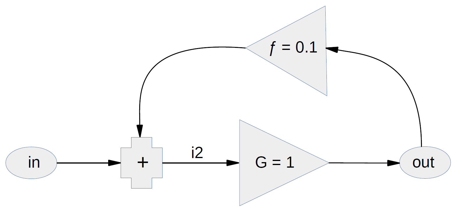
(Gee, I wish we could still get images to show in our comments on this blog!)
There’s no need to distinguish between perturbation components and the whole signal. The system “feeds back” a fraction ƒ of the output, and sums it with the input; call the sum i2. That sum, multiplied by the open-loop gain (1.0 in our simple example) becomes the output.
As Joe says, the algebra is trivial:
in = input
out = output
G = open-loop gain (assume 1.0 for simplicity)
ƒ = feedback (shown as +10%)
i2 = in + (ƒ × out)
out = i2 × G
= G × (in + (ƒ × out))
assume G = 1, then:
out = in + (ƒ × out)
out – (ƒ × out) = in
out × (1 – ƒ) = in
out = in / (1 – ƒ)
As you can see, in general, in a linear system, a feedback ƒ causes a “compounded” net amplification (or attenuation, if ƒ is negative) which multiplies the original effect by 1/(1-ƒ).
if ƒ = +10% then out = in / 0.9 = 1.11111… × in
if ƒ = +50% then out = in / 0.5 = 2 × in
if ƒ = –50% then out = in / 1.5 = 0.66666… × in
etc.
A common misconception is that positive feedbacks necessarily “run away,” and make a system unstable. That is incorrect. Positive feedbacks of less than 100% don’t make a system unstable.
Caveats: In practice, delays in the feedback path may mean that the full amplification effect of a positive feedback isn’t immediately seen. Also, these calculations assume linearity, but most systems are not perfectly linear, though many are approximately linear over ranges of interest.
Feedbacks are at the center of the climate debate. The direct warming effects of anthropogenic greenhouse gas emissions are known to be small, but climate alarmists believe that those slight warming effects will be multiplied dramatically through positive feedbacks, with catastrophic consequences.
There’s scant evidence of that. The best evidence is that manmade climate change is modest and benign, and CO2 emissions are beneficial, rather than harmful.
Thanks for the clear summary.
By the way, your diagram shows up on the emails this site sends to people who request notification.
This treatment applies only to simple, static-gain recirculation of some quantity, typical of process engineering. This usually involves some time delay between input and system output.
The far more general meaning of feedback, as encountered in control systems, involves frequency-dependent transfer functions of the form H/(1-GH), where H is the open-loop transfer and G is the feedback transfer–which is typically accomplished instantaneously and without drawdown of output power. There are rigorous stability criteria (q.v.) for such control systems, due to Nyquist in the linear case and to Lyapunov in the nonlinear, which are nowhere mentioned here.
“A common misconception is that positive feedbacks necessarily “run away,” and make a system unstable. That is incorrect. Positive feedbacks of less than 100% don’t make a system unstable.”
Positive feedback *does* necessarily cause “run away”. Any system where the feedback adds to the input and where the open loop gain of the system is greater than zero will result in run away.
Assume an open loop gain of .5 and a positive feedback of .5. (a feedback less than 100%)
input output feedback
1 .5 .25
1.25 .625 .3125
1.5624 .78125 .390625
1.953025
Any system where the net feedback is positive is unstable. In an electronic amplifier you get an ever increasing output until a physical limit of the real world is reached, i.e. an oscillator.
This means that for Earth there has to be a net feedback that allows the system to be stable. That implies that the net feedback is less than or equal to zero. Negative feedback still allows the output to follow the input in some manner. That, of course, also implies that the temperature of the Earth is dependent on the energy input into the system from the sun. If the energy input goes up the temperature goes up. If the energy input goes down then the temperature goes down.
If the energy into the Earth’s system isn’t balanced by the energy out of the Earth’s system that implies a positive feedback mechanism, i.e. an energy storage mechanism in the Earth’s system. But we know that can’t actually be the case or the Earth would have long ago become a molten rock floating in space since the Earth is not so different today than it has been in the past.
Of course the Earth isn’t an electronic system. Feedback mechanisms act slowly in the Earth’s system thus allowing for wide natural variations. But those feedback mechanisms have to trend toward being negative feedback in some form or another in order to have a somewhat stable system. If that wasn’t the case then we wouldn’t be here arguing over whether we are doomed by man’s actions.
If the climate models are dominated by a positive feedback mechanism that is accurate for the next 100 years then the models should be accurate for the next 1000 years or 1,000,000 years as well. If they aren’t accurate over the long term then they probably aren’t accurate over the short term either.
I think you have missed a step or two. If when you begin the input,
If f = +50% then out = in / 0.5 = 2 x in, but now the feedback is +50% of (2 x in). The output becomes out = (2 x in) / 0.5 = 4 x in. This continues until the power supply ca no longer meet the need.
It doesn’t matter what the feedback % is, the output will increase until the power supply runs out of juice. And, this happens quickly. The upshot? Why has higher CO2 values not caused runaway feedback in the past?
“Positive feedbacks of less than 100% don’t make a system unstable.”
Positive feedback less than 100% can cause instability since it’s the combination of positive feedback and open loop gain that’s important. The stability criteria is that the closed loop gain, g, must be positive and finite. It becomes negative when the reciprocal of the open loop gain, 1/Go, is smaller than the feedback fraction, f and is infinite when f == 1/Go. This is clearly illustrated by the gain equation, 1/Go = 1/g + f.
The climate feedback model has unit open loop gain when modeled as solar power in and surface emissions out, while the open loop gain is meaningless when the output is an incremental change in the surface temperature. This is because you can’t multiply W/m^2 by a dimensionless constant and get a temperature change in degrees and by its definition, the open loop gain is a dimensionless constant.
Very thought provoking contribution, Joe. I always learn something from your discussions about feedback. It will take a long while to absorb, but several thoughts occur immediately.
First, personally I really hate the use of temperature feedback because it implies odd things. I find that it makes the whole discussion more burdensome. Temperature is not an input to the system. It is a response to the current input and output of energy, fully considering possible storage, and it may represent a steady state or a transient condition. It just seems more reasonable to use true inputs and outputs, and view temperature as a setting or parameter of the “plant” representing the current Earth and its climate system. Addition of CO2 is not a feedback, not a forcing, but rather a disturbance to the plant. Climate sensitivity becomes a partial derivative in this view, and so forth.
Second, feedback systems rarely include the power which enables operation of the plant. In the case of an electronic circuit this would be the power supply which we imagine to supply a fixed voltage no matter what. Thus, people speak of a circuit running to the rails, but this comes from an important consideration that is outside the whole discussion of feedback. It seems to me that conservation of energy takes a back seat in these feedback discussions. Instead the first and second laws should be setting up front, with the second law behind the wheel.
Third, related to the second point is the concept of a limit to thermal run-a-way. As you say,
The second law of thermodynamics provides an obvious limit–the Earth cannot become hotter than the emission temperature of the Sun. Not very comforting. Such a world would be one so well insulated against LW loss that it only exchanges radiant energy through a window at visible wavelengths. Even albedo doesn’t matter for such a world. Luckily I have taken historical geology, and read enough of the subject, to recognize that the plant representing our climate system has had some extreme disturbances in the past, but its temperature has remained within surprisingly narrow bounds, unlike, say, Venus. This, I think is a comforting observation.
I agree with you about taking temperature as the input—which I referred to above as the temperature-input view. Indeed, I went back and forth about whether to include something in the head post about how non-physical that view is. Commenter kribaez had justifiably taken me to task on another thread for tacitly reinforcing acceptance of that view, and a comparison of the forcing- and temperature-input feedback-ratio graphs would have been a good place to make that comment; such a comparison would show how artificial the temperature-input view is.
And that discussion would have been okay for a few of the regulars like you, kribaez, Greg, and I’m sure a few others I can’t think of at the moment. But the comments above show that the post was already too mathematical for most of the readership. And, frankly, if someone else had written the post, the length it had without that discussion would already have taxed my own attention span.
Moreover, there’s another reason for not addressing it: what Lord Monckton contended he’d achieved is a formal mathematical proof. However physically misleading we may think his temperature-input view is, it’s internally consistent mathematically. So perhaps the comment would have been inapposite.
As to what you said about which quantities are inputs and which are instead parameters or setpoints, etc., I think I understand your view. But the head post’s purpose was to accept Lord Monckton’s entire-signal rule for the sake of argument and show that nothing he identified in “the mathematics of feedback” thereby ruled out a high ECS value without begging the question. Moreover, forcing is the input in the view that “official climatology” takes. So I’m of the opinion that treating the views I did was appropriate to the purpose.
I don’t really understand the relevance of your second thought, so what I’m going to say here is probably irrelevant. But, again, Lord Monckton claimed he’d arrived at a mathematical proof, which leaves little room for physics. When you think about it, moreover, the First and Second Laws don’t constrain us all that much if we’re taking about temperature and forcing. The surface radiates more power on a steady-state basis than the earth absorbs and re-emits; the First Law isn’t really a limit, because the quantities in question result from multiple-counting the same energy; increasing the atmosphere’s long-wave opacity increases the number of times the same power is counted.
As to your third thought, I did indeed rather gloss over the limits question. But, frankly, I hadn’t thought through all that could have been said about it. Anyway, we were already out in the never-never land of tipping points. So, well, I left that topic to others.
Joe, it was a comment you made to me on these threads some years ago that finally got me to recognize the different view points of temperature versus energy feedback, and made me think a bit more deeply about feedback as a hueristic for analyzing climate.
This is a very good contribution in that it epitomizes the point Feynman was making in that quotation of his I alluded to some weeks ago–the one about taking an argument to completion to see if it really explains anything. Monckton, et al’s, idea as some sort of proof is susceptible to just the sort of analysis you gave. It is complex enough to take me a time to absorb it.
Nick’s allusion to state space models (he may not have used that term) in his “demystifying” contribution back in June was the first time I recall anyone suggesting this fruitful alternative to feedback models, and I had thought of combining this idea with some analysis of Monckton’s contribution. There is no need for that now. However, what state space models do is explicitly separate the physics (the dynamics) of a problem from the process of making observations, which is a view point climate science could use. I just haven’t come up with a good vehicle for illustrating this; and lately I have gotten distracted by a project of finding Eppley radiometers at auctions and putting them back in use.
My second comment is not especially deep. It is no more than a suggestion that the solution to a problem involving feedback can possibly be dependent on unstated assumptions. An assumption that a power supply can deliver whatever the model system demands and still maintain a fixed voltage is one such. Or running to the rails, as people said on the thread is another–it doesn’t come from the model but from something unstated. A better generic example perhaps is the impulse-momentum view of collisions. In this case the assumptions regarding magnitude of force times time interval should depend on the limits of material properties, which we often neglect in a simple model. Our solution might then suggest things that can’t realistically happen.
At any rate, thank you for taking the time to think so thoroughly about this.
Kevin,
I really liked your first comment in toto, but for a partial answer to your second comment, please see my response to Joe below. You are, I regret to say, one of the few people on this thread who might actually understand what I am talking about.
Joe,
You and I have been exchanging comments on sundry questions for about 10 years now. (In case you didn’trealise that, I posted articles for several years on Lucia’s Blackboard starting in 2009, under the pseudonym Paul_K, and you made some interesting and challenging comments at that time querying convolution vs superposition (yes, they are the same thing). We also exchanged views on the validity of Robert Brown’s article on the vertical temperature gradient for a transparent atmosphere, as well as several other matters. I understood in a later exchange why you were focused on the contradictions in Brown’s argument arising from “a small temperature gradient” as a hard vacuum is approached. ) The point about this is that I feel that I know who you are as a scientist and a logician.
You have a fine mind and the soul of a mathematician, despite your time invested as a lawyer focused on technical matters. Mathematicians are perfectly comfortable working within the restricted confines of a space defined by its axioms. All of my friends with mathematical souls love the elegance and beauty of reductio ad absurdum proofs – no matter that the contradiction may seem like a fragile puff of air, its existence is sufficient unto itself to complete a mathematical proof. It turns the fragile contradiction into a solid irrefutable mathematical certainty, since the axiomatic space is well defined. Assume A, show a contradiction while following the axiomatic logic, then this proves (not A). For a mathematician, it can be like tasting a fine wine or appreciating a work of art.
What I discovered in decades of working with other people was that very few of them recognise the definitive nature of such mathematical logic or appreciate its beauty. This includes people of great intelligence in certain attributes, but who are uncomfortable in, or resistant to, accepting assumptions as hard borders to the logical framework. In real life, moving the assumptions to recharacterise a problem is an important way, and sometimes a valid way, to redefine a problem. To convince them, you have to speak into the listening, and mathematical logic is not always the most effective approach.
So I will continue gently to chide you over acceptance of the “temperature as input” model, in order to demonstrate its mathematical problems. If you look at the responses to date, you still have people who believe:-
That temperature is an input to a feedback process rather than a state variable.
That there is a net positive feedback in the sytem, ignoring the arbitrary choice of Planck response as a reference temperature.
That Official Climatology (“OC”) has actually used a control theory model for prediction of ECS.
That OC does not base all of its calculations on absolute temperature, as opposed to incremental temperature.
That, even though Monckton’s model may not be perfect, there might exist a better control analogue for a temperature-input to temperature-output feedback process if only we look hard enough.
Given all of the above, I will (gently) repeat my suggestion that your argument -no matter how rigourous it might be – is the wrong one to use. Try telling your wife “Let us suppose you have a fat ass…” and see whether she accepts it as an assumptive prelude to a very logical proposition.
Warmest regards in any case.
I appreciate the kind words. And, yes, I do recall some of our mathematical discussions. They were among the few bright spots on the Web, which as a source of worthy interlocutors has proved to be disappointing. (But I’m a little surprised that I was dogmatic about nomenclature; I’m usually not. Yes, I tend to think of convolution as only an application of superposition, but nothing much turns on whether it gets accorded the broader meaning. I must have been off my feed.)
Anyway, you’re certainly right that the proof by contradiction above didn’t get through to too many readers. I had actually tried to get WUWT to run a simpler post, one that graphically exposed Lord Monckton’s theory as just bad extrapolation. But that post got spiked; Mr. Watts seems to have been taken in by Lord Monckton’s theory, so he probably concluded that what I said had to be snake oil. This time I therefore avoided something that direct and instead framed the head post as expanding upon Mr. Stokes’.
So this rather oblique approach seemed worth a try. No, it wasn’t optimal, but it got published.
“Yes, I tend to think of convolution as only an application of superposition, but nothing much turns on whether it gets accorded the broader meaning. I must have been off my feed.” Nothing so mundane, as I recall. Analytically, the two integral equations are identical, and you were not challenging that. You were querying, inter alia, the “half-step” time truncation error arising from use of the superposition form – which had me scurrying back to do a direct comparison of cumulative error from numerical solutions of (both) convolution integral and superposition integral against each other and against an analytic solution. A useful challenge, since the diversion led me subsequently to adapt the solution routine I was using in a rather more sophisticated emulation.
Yes, temperature feedback has no physical significance. The feedback fraction is the fraction of output power (net surface emissions) that becomes becomes the feedback power which when added to the forcing power offsets the output power. It’s definitely not something to be implied by a non physical dimensional constant that linearly converts an incremental temperature change into W/m^2 of feedback power. This level of obfuscation is what seems to confuse many by burying necessary details.
Another way to explain the missing power supply is that in an audio amplifier, the output power comes from the implicit power supply (power cord), while for the climate system, the output power originates from the forcing power. As a consequence, COE must be applied between the forcing input and emissions output. Bode’s simplifying assumption of an implicit power supply precludes the need to conserve energy between the input and output of the gain block which otherwise significantly complicates the analysis. Conserving energy between the input and output of the gain block must be applied to the climate feedback model, but is not.
My feeble old brain keeps thinking that using Bode as a climate model requires the sun to change its
output if the earths “impedance ” changes ….
but IMO only the reception of the suns energy changes …
and that leaves far less “room” for temperature change .
“In the case of an electronic circuit this would be the power supply which we imagine to supply a fixed voltage no matter what.”
That’s a simplification. You can run a circuit from a supply with impedance. Or even from a fixed current source. And that is closer to our situation. The power supply is the 240 W/m2 that is delivered to the surface, and has to return to space, generating temperature differentials as it goes. We are sensitive to those temperatures.
The ideal voltage source has low impedance, so you can draw current at will. The ideal current source has infinite impedance, so it will deliver the current whatever the voltage. Insolation is high impedance – as you say, it isn’t until you get towards solar temperature that this is an issue.
Nick,
NO NO NO. Why do you insist on being so wrong despite being corrected numerous times. The 240 W/m^2 from the Sun is the forcing, not the implicit power supply and it can not be both. Why do you think it can? Do you deny that the 240 W/m^2 from the Sun is forcing?
Each and every W/m^2 from the Sun is forcing power, not just the next one as claimed by the IPCC and each W/m^2 of solar forcing, including the next one, all of which are arriving at the same time MUST have the same effect on the average. For some reason, this fundamental constraint of COE is ignored. This is a high school physics type of error and not something that ostensibly intelligent scientists should have made, but they did owing to confirmation bias and the requirement for a large effect from CO2 emissions, regardless of first principles constraints.
This incremental bullshit that Schlesinger introduced with his feedback model in order to fudge around the linearity constraint is so wrong that if Schlesinger wasn’t dead, he should be embarrassed for making such a stupid mistake. Based on my numerous conversations with him and Mike MacCraken (who reviewed the Schlesinger paper), neither was ever able to adequately justify the analysis, both knew about the errors because I showed them how it was wrong, but they stood by the mistakes because without them, the ECS would be too small to worry about which would undermine their cause. This is not how science is supposed to work.
“Based on my numerous conversations with him and Mike MacCraken (who reviewed the Schlesinger paper), neither was ever able to adequately justify the analysis, both knew about the errors because I showed them how it was wrong, but they stood by the mistakes because without them, the ECS would be too small to worry about which would undermine their cause. This is not how science is supposed to work.”
Thanks for that look into the dark soul of climate pseudo-science. They’ll simply never admit they’re wrong and undermine “The Cause,” or kill the “Golden Goose” of “funding” that would surely vanish the minute they admitted how much bullshit their so-called “science” is based on.
What I find most questionable in Joe Born’s article is the comment or assumption near the beginning:
“The perturbation components satisfy equations, but are proportional to the perturbation. You can’t mix them. This is the basic flaw in Lord Monckton’s recent paper.”
The writer here says he was inspired by Nick Stokes earlier discussion, and is in fact repeating the same point. Not coincidentally, this is the same point that Lord Monckton says is not only wrong, Monckton’s claim is that this emphasis on amplifying a perturbation component is what most climate theorists typically assume in the first place!
In other words, the regular theorists tend to assume some sort of amplification of whatever steady state *difference* they may think is implied initially from an initially assumed change in conditions? This is the general sort of assumption that Monckton says is wrong!
Now one thing I have to recognize in thinking about this is the fact that models of reality tend to be their own “little world” one way or another, and how hard it is, you see, to connect the supposedly realistic model with the likely behavior of the *actual” real world. On top of *that* basic uncertainty there is also the point that I am not at all sure myself that climate theorists always even think in terms of amplifying some sort of difference from some sort of (perhaps mythical) perfect equilibrium? In visualizing the IR resisting and “clouds vs sunshine” effects as best *I* can, I find that I *do* think of Lord Monckton’s portrayal of the wrongness of the “bad” way of treating feedback (i.e. as “boost the perturbation”), as a more or less plausible criticism by Monckton. In particular, the mathematics of how assumed feedback boosted temperature sensitivity is supposed to raise the earth’s temperature is right there in one’s face as something simple, it shouldn’t be all that confusing! It is hardly even algebra, just multiplication, to say that a factor of three, say, is supposed to be boosting the most basic one degree C difference by three times, to get three degrees!
In some sense, this looks like it may be a kind of hidden assumption, whether theorists always acknowledge it explicitly or not? I note, too, that the presentations here on WUWT *do* tend to focus on this point. In other words, it is the same old mistake, re-iterated!
To put it a slightly different way, if someone wants to amplify a perturbation, a “difference”, well then, “Amplifying a difference from what”, one may ask?
Suppose you know that a rock fell one inch in the last millisecond and you want to estimate how far it will fall in the next millisecond. Would you guess that it will fall (just a hair more than) another inch? Or would you go with half an inch instead because its speed has averaged half an inch per millisecond since it was dropped?
The former answer is the result of basing your estimate on perturbations, i.e., on the one-millisecond time increment and the current speed, without paying attention to total time since the rock was dropped. The latter is Lord Monckton’s way of basing it on entire values, i.e., on the entire lapsed time and entire dropped distance.
Some readers have tended to believe that Lord Monckton has shown that because feedback is involved the answer should be different from the one inch we’d ordinarily think. But why do they believe that?
Suppose the rock is attached to a rocket whose speed depends on continuous feedback using radar measurement of ground proximity or other things? If some sort of feedback control were involved, are you saying that would (or wouldn’t) make any difference at all?
The distance traveled in the next millisecond would still be best approximated by the distance traveled in the last millisecond.
It’s only if the control system so controls the motion as to keep its speed steady that the average speed might also provide a good approximation. As the closed-loop functions above demonstrate, nothing in feedback theory requires that feedback produce such a result.
The idea that climate strives for equilibrium seems odd in light of this:
Anyone spending time reading research regarding the past 800,000 years can clearly see that long term climate is a wicked problem that would likely entail a number of different mathematical models depending on what catalysts are present at any given time and their waning and waxing power to influence.
Zooming in on the modern period is far more complex:
I present these two zoomed out and zoomed in temperature reconstructions to propose that understanding both mathematically may not be our best use of time. Clearly one of the two climate views is insignificant.
Interesting graphs!
Pardon me, that second graph has me scared now … got to go buy a really big parka..
In actuality, feedback over a wide range of temperatures MUST be strongly negative.
Consider Gough’s formula for the Sun’s luminosity over time,
https://agupubs.onlinelibrary.wiley.com/doi/full/10.1029/2011RG000375
And anything OTHER than a large negative feedback will result in an Earth frozen solid about 550 million years ago- the time of the Cambrian explosion.
I think Ou was right, and strong negative water in its three phases is what has maintained relative stability over Earth’s history.
https://journals.ametsoc.org/doi/full/10.1175/1520-0442%282001%29014%3C2976%3APBOTES%3E2.0.CO%3B2
Regarding ‘the “official climatology” ECS value, Delta E(2xCO2) =3.35 K, and the value Delta R{2xCO2) =1.05 K’: I’ve always heard 3.7 W/m^2 per 2xCO2 and 1.1 K per 2xCO2 respectively as the usual figures. The lower figures were derived from Andrews 2012.
The tipping point never happens because as atmospheric temperature increases, the amount of collisions between CO2 and N2/O2 increases exponentially. Therefore convection gets rid of the heat before it has a chance to radiate downwards. Only low level clouds provide any substantial DWIR as can be witnessed at nightime when the surface air can be as much as 11C warmer with low level clouds as compared to the same conditions without clouds. Thus there are actually 2 temperature regimes. One is the overall temperature of the earth’s adiabatic compression temperature and the 2nd regime is a local one caused by clouds and water vapour. The input to temperature caused by CO2 is so low as to be unmeasurable as witnessed by NASA’s inability to measure DWIR in an arid desert at nighttime.
I am not convinced that feedback is the proper system description of climate to begin with. The sun is the energy input or in other words the power supply. The laws of thermodynamics control the load/service curve. The “load” point is determined by bias. The kicker is that the bias has a number of “frequency” dependent components like CO2, water vapor, winds, methane, etc. and that they are also inter-related. Throw in geography and it gets complicated really quickly.
Figure all this out and you’ll be able to get a temperature out for a given set of conditions.