Guest Essay by Kip Hansen
 It seems that every time we turn around, we are presented with a new Science Fact that such-and-so metric — Sea Level Rise, Global Average Surface Temperature, Ocean Heat Content, Polar Bear populations, Puffin populations — has changed dramatically — “It’s unprecedented!” — and these statements are often backed by a graph illustrating the sharp rise (or, in other cases, sharp fall) as the anomaly of the metric from some baseline. In most cases, the anomaly is actually very small and the change is magnified by cranking up the y-axis to make this very small change appear to be a steep rise (or fall). Adding power to these statements and their graphs is the claimed precision of the anomaly — in Global Average Surface Temperature, it is often shown in tenths or even hundredths of a Centigrade degree. Compounding the situation, the anomaly is shown with no (or very small) “error” or “uncertainty” bars, which are, even when shown, not error bars or uncertainty bars but actually statistical Standard Deviations (and only sometimes so marked or labelled).
I wrote about this several weeks ago in an essay here titled “Almost Earth-like, We’re Certain”. In that essay, which the Science and Environmental Policy Project’s Weekly News Roundup characterized as “light reading”, I stated my opinion that “they use anomalies and pretend that the uncertainty has been reduced. It is nothing other than a pretense. It is a trick to cover-up known large uncertainty.”
Admitting first that my opinion has not changed, I thought it would be good to explain more fully why I say such a thing — which is rather insulting to a broad swath of the climate science world. There are two things we have to look at:
- Why I call it a “trick”, and 2. Who is being tricked.
WHY I CALL THE USE OF ANOMALIES A TRICK
What exactly is “finding the anomaly”? Well, it is not what it is generally thought. The simplified explanation is that one takes the annual averaged surface temperature and subtracts from that the 30-year climatic average and what you have left is “The Anomaly”.
That’s the idea, but that is not exactly what they do in practice. They start finding anomalies at a lower level and work their way up to the Global Anomaly. Even when Gavin Schmidt is explaining the use of anomalies, careful readers see that he has to work backwards to Absolute Global Averages in Degrees — by adding the agreed upon anomaly to the 30-year mean.
“…when we try and estimate the absolute global mean temperature for, say, 2016. The climatology for 1981-2010 is 287.4±0.5K, and the anomaly for 2016 is (from GISTEMP w.r.t. that baseline) 0.56±0.05ºC. So our estimate for the absolute value is (using the first rule shown above) is 287.96±0.502K, and then using the second, that reduces to 288.0±0.5K.”
But for our purposes, let’s just consider that the anomaly is just the 30-year mean subtracted from the calculated GAST in degrees.
As Schmidt kindly points out, the correct notation for a GAST in degrees is something along the lines of 288.0±0.5K — that is a number of degrees to tenths of a degree and the uncertainty range ±0.5K. When a number is expressed in that manner, with that notation, it means that the actual value is not known exactly, but is known to be within the range expressed by the plus/minus amount.

This illustration shows this in actual practice with temperature records….the measured temperatures are rounded to full degrees Fahrenheit — a notation that represents ANY of the infinite number of continuous values between 71.5 and 72.4999999…
It is not a measurement error, it is the measured temperature represented as a range of values 72 +/- 0.5. It is an uncertainty range, we are totally in the dark as to the actual temperature — we know only the range.
Well, for the normal purposes of human beings, the one-degree-wide range is quite enough information. It gets tricky for some purposes when the temperature approaches freezing — above or below frost/freezing temperatures being Climatically Important for farmers, road maintenance crews and airport airplane maintenance people.
No matter what we do to temperature records, we have to deal with the fact that the actual temperatures were not recorded — we only recorded ranges within which the actual temperature occurred.
This means that when these recorded temperatures are used in calculations, they must remain as ranges and be treated as such. What cannot be discarded is the range of the value. Averaging (finding the mean or the median) does not eliminate the range — the average still has the same range. (see Durable Original Measurement Uncertainty ).
As an aside: when Climate Science and meteorology present us with the Daily Average temperature from any weather station, they are not giving us what you would think of as the “average”, which in plain language refers to the arithmetic mean — rather we are given the median temperature — the number that is exactly halfway between the Daily High and the Daily Low. So, rather than finding the mean by adding the hourly temperatures and dividing by 24, we get the result of Daily High plus Daily Low divided by 2. These “Daily Averages” are then used in all subsequent calculations of weekly, monthly, seasonal, and annual averages. These Daily Averages have the same 1-degree wide uncertainty range.
On the basis of simple logic then, when we finally arrive at a Global Average Surface Temperature, it still has the original uncertainty attached — as Dr. Schmidt correctly illustrates when he gives Absolute Temperature for 2016 (link far above) as 288.0±0.5K. [Strictly speaking, this is not exactly why he does so — as the GAST is a “mean of means of medians” — a mathematical/statistical abomination of sorts.] As William Briggs would point out “These results are not statements about actual past temperatures, which we already knew, up to measurement error.” (which measurement error or uncertainty is at least +/- 0.5).
The trick comes in where the actual calculated absolute temperature value is converted to an anomaly of means. When one calculates a mean (an arithmetical average — total of all the values divided by the number of values), one gets a very precise answer. When one takes the average of values that are ranges, such as 71 +/- 0.5, the result is a very precise number with a high probability that the mean is close to this precise number. So, while the mean is quite precise, the actual past temperatures are still uncertain to +/-0.5.
Expressing the mean with the customary ”+/- 2 Standard Deviations” tells us ONLY what we can expect the mean to be — we can be pretty sure the mean is within that range. The actual temperatures, if we were to honestly express them in degrees as is done in the following graph, are still subject to the uncertainty of measurement: +/- 0.5 degrees.

[ The original graph shown here was included in error — showing the wrong Photoshop layers. Thanks to “BoyfromTottenham” for pointing it out. — kh ]
The illustration was used (without my annotations) by Dr. Schmidt in his essay on anomalies. I have added the requisite I-bars for +/- 0.5 degrees. Note that the results of the various re-analyses themselves have a spread of 0.4 degrees — one could make an argument for using the additive figure of 0.9 degrees as the uncertainty for the Global Mean Temperature based on the uncertainties above (see the two greenish uncertainty bars, one atop the other.)
This illustrates the true uncertainty of Global Mean Surface Temperature — Schmidt’s acknowledged +/- 0.5 and the uncertainty range between reanalysis products.
In the real world sense, the uncertainty presented above should be considered the minimum uncertainty — the original measurement uncertainty plus the uncertainty of reanalysis. There are many other uncertainties that would properly be additive — such as those brought in by infilling of temperature data.
The trick is to present the same data set as anomalies and claim the uncertainty is thus reduced to 0.1 degrees (when admitted at all) — BEST doubles down and claims 0.05 degrees!


Reducing the data set to a statistical product called anomaly of the mean does not inform us of the true uncertainty in the actual metric itself — the Global Average Surface Temperature — any more than looking at a mountain range backwards through a set of binoculars makes the mountains smaller, however much it might trick the eye.
Here’s a sample from the data that makes up the featured image graph at the very beginning of the essay. The columns are: Year — GAST Anomaly — Lowess Smoothed
2010 0.7 0.62
2011 0.57 0.63
2012 0.61 0.67
2013 0.64 0.71
2014 0.73 0.77
2015 0.86 0.83
2016 0.99 0.89
2017 0.9 0.95
The blow-up of the 2000-2017 portion of the graph:

We see global anomalies given to a precision of hundredths of a degree Centigrade. No uncertainty is shown — none is mentioned on the NASA web page displaying the graph (it is actually a little app, that allows zooming). This NASA web page, found in NASA’s Vital Signs – Global Climate Change section, goes on to say that “This research is broadly consistent with similar constructions prepared by the Climatic Research Unit and the National Oceanic and Atmospheric Administration.” So, let’s see:
From the CRU:

Here we see the CRU Global Temp (base period 1961-90) — annoyingly a different base period than NASA which used 1951-1980. The difference offers us some insight into the huge differences that Base Periods make in the results.
2010 0.56 0.512
2011 0.425 0.528
2012 0.47 0.547
2013 0.514 0.569
2014 0.579 0.59
2015 0.763 0.608
2016 0.797 0.62
2017 0.675 0.625
The official CRU anomaly for 2017 is 0.675 °C — precise to thousandths of a degree. They then graph it at 0.68°C. [Lest we think that CR anomalies are really only precise to “half a tenth”, see 2014, which is 0.579 °C. ] CRU manages to have the same precision in their smoothed values — 2015 = 0.608.
And, not to discriminate, NOAA offers these values, precise to hundredths of a degree:
2010, 0.70
2011, 0.58
2012, 0.62
2013, 0.67
2014, 0.74
2015, 0.91
2016, 0.95
2017, 0.85
[Another graph won’t help…]
What we notice is that, unlike absolute global surface temperatures such as those quoted by Gavin Schmidt at RealClimate, these anomalies are offered without any uncertainty measure at all. No SDs, no 95% CIs, no error bars, nothing. And precisely to the 100th of a degree C (or K if you prefer).
Let’s review then: The major climate agencies around the world inform us about the state of the climate through offering us graphs of the anomalies of the Global Average Surface Temperature showing a steady alarmingly sharp rise since about 1980. This alarming rise consists of a global change of about 0.6°C. Only GISS offers any type of uncertainty estimate and that only in the graph with the lime green 0.1 degree CI bar used above. Let’s do a simple example: we will follow the lead of Gavin Schmidt in this August 2017 post and use GAST absolute values in degrees C with his suggested uncertainty of 0.5°C. [In the following, remember that all values have °C after them – I will use just the numerals from now on.]
What is the mean of two GAST values, one for Northern Hemisphere and one for Southern Hemisphere? To make a real simple example, we will assign each hemisphere the same value of 20 +/- 0.5 (remembering that these are both °C). So, our calculation: 20 +/- 0.5 + 20 +/- 0.5 divided by 2 equals ….. The Mean is an exact 20. (now, that’s precision…)
What about the Range? The range is +/- 0.5. A range 1 wide. So, the Mean with the Range is 20 +/- 0.5.
But what about the uncertainty? Well the range states the uncertainty — or the certainty if you prefer — we are certain that the mean is between 20.5 and 19.5.
Let’s see about the probabilities — this is where we slide over to “statistics”.
Here are some of the values for the Northern and Southern Hemispheres, out of the infinite possibilities inferred by 20 +/- 0.5: [we note that 20.5 is really 20.49999999999…rounded to 20.5 for illustrative purposes.] When we take equal values, the mean is the same, of course. But we want probabilities — so how many ways can the result be 20.5 or 19.5? Just one way each.
NH SH
20.5 —— 20.5 = 20.5 only one possible combination
20.4 20.4
20.3 20.3
20.2 20.2
20.1 20.1
20.0 20.0
19.9 19.9
19.8 19.8
19.7 19.7
19.6 19.6
19.5 —— 19.5 = 19.5 only one possible combination
But how about 20.4 ? We could have 20.4-20.4, or 20.5-20.3, or 20.3-20.5 — three possible combinations. 20.3? 5 ways 20.2? 7 ways 20.1? 9 ways 20.0? 11 ways . Now we are over the hump and 19.9? 9 ways 19.8? 7 ways 19.7? 5 ways 19.6? 3 ways and 19.5? 1 way.
You will recognize the shape of the distribution:

As we’ve only used eleven values for each of the temperatures being averaged, we get a little pointed curve. There are two little graphs….the second (below) shows what would happen if we found the mean of two identical numbers, each with an uncertainty range of +/- 0.5, if they had been rounded to the nearest half degree instead of the usual whole degree. The result is intuitive — the mean always has the highest probability of being the central value.

Now, that may seem so obvious as to be silly. After all, that’s that a mean is — the central value (mathematically). The point is that with our evenly spread values across the range — and, remember, when we see a temperature record give as XX +/- 0.5 we are talking about a range of evenly spread possible values, the mean will always be the central value, whether we are finding the mean of a single temperature or a thousand temperatures of the same value. The uncertainty range, however, is always the same. Well, of course it is! Yes, has to be.
Therein lies the trick — when they take the anomaly of the mean, they drop the uncertainty range altogether and concentrate only on the central number, the mean, which is always precise and statistically close to that central number. When any uncertainty is expressed at all, it is expressed as the probability of the mean being close to the central number — and is disassociated from the actual uncertainty range of the original data.
As William Briggs tells us: “These results are not statements about actual past temperatures, which we already knew, up to measurement error.”
We already know the calculated GAST (see the re-analyses above). But we only know it being somewhere within its known uncertainty range, which is as stated by Dr. Schmidt to be +/- 0.5 degrees. Calculations of the anomalies of the various means do not tell us about the actual temperature of the past — we already knew that — and we knew how uncertain it was.
It is a TRICK to claim that by altering the annual Global Average Surface Temperatures to anomalies we can UNKNOW the known uncertainty.
WHO IS BEING TRICKED?
As Dick Feynman might say: They are fooling themselves. They already know the GAST as close as they are able to calculate it using their current methods. They know the uncertainty involved — Dr. Schmidt readily admits it is around 0.5 K. Thus, their use of anomalies (or the means of anomalies…) is simply a way of fooling themselves that somehow, magically, that the known uncertainty will simply go away utilizing the statistical equivalent of “if we squint our eyes like this and tilt our heads to one side….”.
Good luck with that.
# # # # #
Author’s Comment Policy:
This essay will displease a certain segment of the readership here but that fact doesn’t make it any less valid. Those who wish to fool themselves into disappearing the known uncertainty of Global Average Surface Temperature will object to the simple arguments used. It is their loss.
I do understand the argument of the statisticians who will insist that the mean is really far more precise than the original data (that is an artifact of long division and must be so). But they allow that fact to give them permission to ignore the real world uncertainty range of the original data. Don’t get me wrong, they are not trying to fool us. They are sure that this is scientifically and statistically correct. They are however, fooling themselves, because, in effect, all they are really doing is changing the values on the y-axis (from ‘absolute GAST in K’ to ‘absolute GAST in K minus the climatic mean in K’) and dropping the uncertainty, with a lot of justification from statistical/probability theory.
I’d like to read your take on this topic. I am happy to answer your questions on my opinions. Be forewarned, I will not argue about it in comments.
# # # # #
I’ve always used anomaly analysis to identify anomalous data, where in this case, the anomalous errors being identified are methodological.
There can be no doubt that the uncertainty claimed by the IPCC and its self serving consensus is highly uncertain. Consider the claimed ECS of 0.8C +/- 0.4C per W/m^2 of forcing. Starting from 288K and its 390 W/m^2 of emissions, this means that 1 W/m^2 of forcing can increase the surface emissions from between 2.25 W/m^2 and 6.6 W/m^2, where even the lower limit of 2.25 W/m^2 of emissions per W/m^2 of forcing is larger than the measured steady state value of 1.62 W/m^2 of surface emissions per W/m^2 of solar forcing. Clearly, the IPCC’s uncertain ECS, as large as the uncertainty already is, isn’t even large enough to span observations!
“… rather than finding the mean by adding the hourly temperatures and dividing by 24, we get the result of Daily High plus Daily Low divided by 2. ”
Taking the Daily High plus the Daily Low and dividing by 2 can easily give a trend in the opposite direction of actual temperatures. IOW, a set of these values could show a warming trend when it is actually cooling.
Many times I have worked outside all day for several days in a row. Often my perception was that one particular day was cooler than the others, because most of that day was partly cloudy.
Often, when I see the weather record for those days, I am surprised to learn that the record shows the day I thought was cooler was actually just as warm, and sometimes warmer, than the other days. This happens when there is a short period of full sunshine during mid-afternoon.
Even though many hours of that day were cooler than the corresponding hours of the other days, that day got recorded as just as warm, and sometimes warmer, than the other days.
SR
That is why a world average temperature is a nonsense… too many variables and too many adjustments have been made. One can only get a reliable record from a set of single sources that are comparable and which have been obtained using the same method. For the world the oceans are the only places always at sea level so land based measures have to be adjusted for altitude to be comparable and of course land radiates more heat which bounces back off clouds than sea. It’s all nonsense based on groggy data.
One can only really look at one place and compare it over time, so long as the Stevenson screen remains in an open place away from development and close by trees.
That feeling of being cooler is because you are in the shade of the clouds right? Weather thermometers are always in the shade, so are not affected much by the cloud cover per-se…
Mark ==> The phenomena that Steve is mentioning is related to determining the “Daily Average” temperature from the median of the Max/Min for the day. To a relatively cool day with a short period of high temps (a spike in late afternoon, say) and be reported as “warmer” (Daily Average) than a day with the same Min but an evenly moderately warm afternoon with no temp spike.
The cooler day was cooler most of the time but is reported higher because of a temp spike.
co2 and Steve ==> Both examples of what happens when we use the Hi+Low/2 method — pretending it is the daily average.
This problem is magnified throughout the rest of the “average temperature system.”
Hi Kip,
quick question, are the daily min and max actually recorded in the data archives or just the midpoint? Plotting both min/max and how they develop over time would give a better indication of where the climate might be going, at least in my opinion but i have never seen such a graph.
Best,
Willem
Willem ==> Usually the Min/Max are recorded along with the Daily Average. Modern AWS/ASOS stations record a great deal more detail, but still figure the Daily Average the same way. There are some such graph out there somewhere — but in my opinion are only useful at a local level.
It would seem to be seasonally exaggerated, longer cold nights in winter would average colder with 24 hourly readings averaged, as would summer’s long days be actually warmer than recorded. The real difference between summer and winter is much larger than what is recorded by averaging two daily measurements, which is all our records show.
Do I not recall correctly, in a number of articles on adjustments to temperature measurements, there is always listed a time of day adjustment?
If only the min and max temperatures are recorded, how could any adjustment for time be relevant?
Andy ==> “Understanding Time of Observation Bias” – – – for what it is worth.
Kip,
Ideally one would replicate the work to verify its consistency and accuracy but I believe I get the idea, at least to the extent that there are different results from the same data depending on how one uses the data. The TOB adjustment described may be done entirely honestly and with good intentions but the result is still a calculated guess of what might have happened because of how things were done, not actually know values, no?
Andy ==> I am suspicious of the standardized size of the adjustment — if you have the energy and the time, you might take some modern complete station record with six minute values and calculate the Daily Average (Max + Min/2) using all 24 of the hours of the day as the start of day and see if the change in Daily average is really as great as they say.
“not actually know values, no?”
Values are known, as explained here. The time and amount of TOBS is known. The effect can be deduced from the diurnal pattern. There is often hourly or better data now at the actual site, from MMTS; if not, there are usually similar MMTS locations nearby.
Averaging temperature is misleading at best no matter how many samples are used. To compute averages with any relation to the energy balance and the ECS, you must convert each temperature sample into equivalent emissions using the SB Law, add the emissions, divide by the number of samples and convert back to a temperature by inverting the SB Law. 2 samples per day are nowhere near enough to establish the average with any degree of certainty, even if they are the min and max temperatures of the day. If the 2 samples are provided with time stamps allowing the change from one to another to be reasonably interpreted, it gets a little better, but is still no where near as good as 24 real samples per day.
It’s worse than that. Temperature is an intensive property of the point in time and space the measurement was taken. Averaging that with other points in time and space doesn’t give you anything meaningful.
Yes, isn’t that convenient? Allows them to continue to bray about nothing for far longer that way.
Thomas Homer
I wonder … for the majority of Earth’s surface
where there are no thermometers, and the
temperature numbers are wild guesses,
by government bureaucrats with science degrees,
do they wild guess a Daily High and Daily Low number
for each “empty grid”, or do they save time and
just wild guess the Daily Average, ‘
or save even more time
and just wild guess the Monthly Average
for that grid?
That question has been keeping me up at night.
No other field of science would take the
surface temperature numbers seriously,
and it always amazes me when people here,
who are skeptics, and should know better,
do just that.
Surface “temperature numbers” =
Over half wild guess “infilling” plus
Under half “adjusted raw data”
No real raw data are used in the average.
When you “adjust” data, you are claiming
the initial measurements were wrong,
and you believe you know what they
should have been.
That’s no longer real data.
“Adjustments” can make
raw data move closer,
or farther away,
from reality.
Interesting that having weather satellite
data, that requires far less infilling,
and correlates well with weather balloon data,
that any people here would use the horrible
surface temperature “data”
that DOES NOT CORRELATE WELL
with the other two measurement methodologies.
That’s something I’d expect only of Dumbocrats
— They’ll always choose the measurement methodology
that produces the scariest numbers !
Because truth is not a leftist value.
Thanks for the interesting and informative article, Kip, but shouldn’t the error bars on your ‘Global mean temperatures from reanalyses’ Br twice as long as you have shown? Each one appears to me to be equal to about 0.5 degrees on the left hand scale, not 1 degree (+/-0.5 degrees).
BoyfromTottenham ==> Well Done, sir. You have caught me using the wrong version of this graph –with the wrong Photoshop layers showing. I”ll replace it with an explanation in the text.
I do so appreciate readers you really look at the graphs and words — and thus see mistakes that I have missed.
Kip, I will take you up on your request.
First, degrees C means Celsius not Centigrade. But that is too easy.
I appreciate that you have made a good presentation, but you have a problem.
“These “Daily Averages” are then used in all subsequent calculations of weekly, monthly, seasonal, and annual averages. These Daily Averages have the same 1-degree wide uncertainty range.”
This is not correct. That is not how uncertainties are carried forward through calculations. You could perhaps look at some worked examples in Wikipedia which for mathematical things is a pretty reliable source.
See here for examples:
https://en.m.wikipedia.org/wiki/Propagation_of_uncertainty
I will first present an oversimplified example of adding two numbers with an uncertainty of half a degree: 20±1 + 20±1 = 40±2
Possible values are 19+19 = 38, up to 21+21 = 42
This ±2 is not the correct answer, but it is a demonstration that adding two equally uncertain numbers doesn’t mean the final uncertainty is from only one, unless the second number is absolutely known, which is not the case with an anomaly.
The correct answer is the square root of the sum of the squares of the two uncertainties.
Square root of (1.0 squared + 1.0 squared) = 1.41
The real answer is 40±1.41
If you want the average, it is 20±0.71 because both values have to be divided by the same divisor so the Relative Error remains the same.
This is the uncertainty of the sum of the two inputs. Similarly, subtraction generates the same increase in uncertainty. Try it.
An anomaly is the result of a subtraction involving two numbers that each have an uncertainty. You do not mention this. Errors propagate. The anomaly does not have an uncertainty equal to the new value because the baseline also has an uncertainty.
Suppose the baseline is 20.0 ±0.5 and the new value is 21.0 ±0.5.
The anomaly is 1 ±0.71. Why? Because the propagated error magnitude is
±SQRT( 0.5^2 + 0.5^2) = ±0.71
In all cases the anomaly has a greater uncertainty than the two input numbers because it involves a subtraction.
Crispin,
I think your math is good for “random” errors. What about “systemic” errors? I think much of what is being pointed out by some here has to do with systemic errors.
Good point , well presented Crispin.
Another point where Kip goes wrong is claiming that the uncertainty of the original measurement can not be reduced: the +/-0.5 is always there.
While it is correct to call this an “uncertainty”, it can also be more precisely described as quantisation error. The smallest recorded change or “quantum” is one degree. No factions. This adds a random error to the actual temperature. A rounding or quantisation error.
Measuring at different times in a day ( min, max ) or at different sites will involved unstructured, random errors. If you average a number of such readings the quantisation errors will be distributed both + and – and of varying magnitudes and will ‘average out’. This allows reducing the expected uncertainty by dividing by SQRT(N), as Crispin does above for N=2.
This is based on the assumption that the errors are “random” or normally distributed. There are other systematic errors but that is a separate question.
If you have sufficiently large number of readings the effect of quantisation error in the original readings will become insignificantly small. There are many other errors involved in this process and the claimed uncertainties are very optimistic. However the nearest degree issue Kip goes into here is not one of them and his claim this propagates is incorrect.
auto-correction. This is not a case of normally distributed errors. The root N factor derives from the normal distribution and is not the correct factor here.
As Kip correctly shows in the article, the distribution is flat and finite. There is just the same change of having a 0.1 error as a 0.5 error. This does not negate that the errors will average out over a large sample and become insignificant.
To say the uncertainty in the mean is +/- 0.5 is to say that there is an equal chance that all values had an error of +0.5 as there was a chance that there was an even mix which averaged out. That is obviously not the case for a flat distribution.
As long that the number of samples is sufficiently large for this theoretical flat distribution to be well represented in the sample the error in the mean will tend to zero. That is where the stats theory comes in in relation to the sample sixe, the expected distribution and the uncertainty levels to attribute to the mean.
Greg
You are violating the Central Limit Theorem which is what the Error in The Mean relies on.
The uncertainty in a measurement is a hard limit based on characterisation and repeatability. This is defined by metrology.
It means that the “resolution” of the sample distribution is +/- 0.5 degrees. To demonstrate identically distributed samples they need to vary by more than this.
You have assumed that other errors are random and follow a similar distribution. The MET Office made the same assumption with SST.
It is an unverified assumption. If applied your data becomes hypothetical and unfit for real life use.
It doesn’t matter how many meaurements you have. It’s like measuring a human hair multiple times with a ruler marked in cms and claiming you can get the value to microns.
Beware of slipping into hypothetical.
Greg, are you sure that “Large Number” theory applies to a measurement of something that changes every minute of every day, with different equipment and in different locations all over the world?
I thought it applied to repetitive measurement of an object.
A catch with temperatures is that, typically, there is only one sensor involved. Each temperature is a sample of one, at one place and at one time. You could use the CLT if you had 30 or more sensors in that Stevenson screen, for that screen’s value; but only for that value. Extrapolation and interpolation add their own errors and uncertainties to the mix. NB that errors and uncertainties are not synonyms. In the damped=driven mathematically chaotic, dynamic system that is Earth’s weather, ceteris paribus will almost always be false.
cdquarles==> You point out one of the fallacies of climate modeling — which attempts prediction of the future by running their models with one factor changing, all else ceteris paribus.
See mine @ur momisugly Dr. Curry’s blog “Lorenz validated” https://judithcurry.com/2016/10/05/lorenz-validated/
These are not repeated measures for the same phenomena, these are singular measures (with ranges) for multiple phenomena (temperature measured at multiple locations).
The reduction in uncertainty by averaging ONLY applies for repeated measures of the (exact) same thing, i.e. the temperature at a single location (at a single point in time).
NOT to the averaging of singular measures for multiple phenomena.
Jaap ==> Yes, exactly right.
Also measurement error is nice to know, but when small to stddev of sample population it hardly matters. What one does when averaging temperatures across the global is asking what is the typical temperature (on that day).
Say you do that with height of recruits for the army. We use a standard procedure to get good results and a nice measurement tool. Total expected measurement error is say 0.5 cm. We measure 20 recruits (not same recruit 20x).
Here are the results:
# height
1 182
2 178
3 175
4 183
5 177
6 176
7 168
8 193
9 181
10 187
11 181
12 172
13 180
14 175
15 175
16 167
17 186
18 188
19 193
20 180
Average 179.85
StDev (s) 7.19
95% range
min max
165.47 194.23
Remember that these are different individuals, so not repeated measures of the same thing, but multiple measures of different things, which are then averaged to get an estimate of the midpoint (average) and range (variance).
Both those min, avg and max still also have that measurement error, but we usually forget all about that because it is so small compare to the range of the sample set.
The Central Limit Theorem gets misunderstood a lot. It doesn’t mean that measuring each temperature a million times yields any different distribution from the base data. That is the accursed error called autocorrelation. Instead, what it means is that if each sample is hundreds of random measurements from the entire overall population, THOSE sample means have a different distribution from the overall population. But that’s never how these samples are taken.
Crispin ==> Caught me with my age showing — “cen·ti·grade
ˈsen(t)əˌɡrād/ adjective adjective: centigrade another term for Celsius.”
As for the rest — you are doing statistics — not mathematics.
We are not dealing with “error” here, we are dealing with temperatures which have been recorded as ranges 1 degree (F) wide. That range is not reduced — ever.
This is not a matter of “propagation of error”.
Kip, cdquarles, A C Osborn, Mickey, Greg and William
There are some good points made above, by which I mean issues are raised that have to be considered when determining the reliability of a calculated result.
The most important to the conversation is that the calculation of an “anomaly” requires subtracting one value with an uncertainty from another value with its own uncertainty and there is a standard manner in which to do this correctly. Invariably the final answer will have a greater uncertainty than the two inputs because we do not know the absolute values.
A separate matter is how the temperature “averages” were produced. Addressing the example given above:
Measure the temperature of one object 30 times in quick succession using the same instrument which has a known uncertainty about its reporting values. The distribution of the readings may be Normal. One could say they will “probably be Normal”.
Let’s assume that the instrument was calibrated perfectly at the start. If the time period is long, perhaps a year, the manufacturer usually provides information on the drift of the instrument so the uncertainty of the measurement can be reported as different from when it was last calibrated.
Now consider using 30 instruments to measure 30 different objects that are 30 different temperatures to find the “average” of a large object like a bulldozer. It is not true to claim that the measurement errors are “Normally distributed” because there is no distribution pattern available for each single measurement. You could assume that the drift of the instruments over time has a normal distribution, but it probably isn’t. So we have two things to address: measurement uncertainty and instrument drift. The first is a random error and the second is a systematic error. The easy answer is the increase the expressed uncertainty with time to accommodate drift and that is what people (should) do.
I cannot possibly present all the considerations that go into the production of a global surface temperature anomaly so let’s stick to the topic of the day.
“Error propagation : A term that refers to the way in which, at a given stage of a calculation, part of the error arises out of the error at a previous stage. This is independent of the further roundoff errors inevitably introduced between the two stages. Unfavorable error propagation can seriously affect the results of a calculation.”
https://www.encyclopedia.com/computing/dictionaries-thesauruses-pictures-and-press-releases/error-propagation
There are no “favourable” error propagations. Unless the calculation involves a constant such as dividing by 100, the uncertainty increases with each processing step. And don’t get me going about the “illegal” averaging averages. The example of the diameter of a human hair and the centimetre ruler is helpful. Using that instrument read to within 1 mm, the diameter of a single hair is 0±0.1 centimetres, every time. That includes the rounding error which is in addition to the measurement uncertainty. Averaging 30, nay, 300 measurements does not improve the result at all.
Claiming to have calculated a global temperature anomaly value with 10 times or 50 times lower uncertainty than for the two values used in the subtraction is hogwash. If the baseline is 20.0±0.5 with 68% confidence and the new value is 20.3±0.5 also with the same confidence index, then the anomaly is 0.3±0.71 [68% CI]. If you want 95% confidence you need a more accurate instrument and more readings for each initial value in the data set being averaged. There is a trend towards doing exactly this: multiple instruments at each site.
Crispin ==> Thanks for your exposition on errors . their propagation, and uncertainty.
Kip,
I just re-read the whole article again and if you have sent it to me for review, I would had insisted on at least a dozen changes. The wording is too casual, given that it attempts to point out something quite technical.
One more example:
“When one calculates a mean (an arithmetical average — total of all the values divided by the number of values), one gets a very precise answer.”
This confuses accuracy and precision. First, these are not multiple measurements of a single thing. Second, the average of a number of readings cannot be more precise than the precision of the contributing values. That would be false precision. In any case, precision has to be stated within a range defined by the accuracy.
What you are alluding to (Willis often does the same thing so don’t feel lonely) is that one can claim “to more precisely estimate” (not “know”) the position of the centre of the range of uncertainty with additional measurements. It is not an increase in the precision or accuracy of the reported value. This is basic metrology, freely abandoned in the climate science community when it comes to anomalies. They are making fantastical claims.
One cannot laugh hard enough at the silly claim that an anomaly is known to 0.05 C using a baseline value subtracted from the current average, both with uncertainties of 0.5 C. They literally cannot do the math. One cannot treat calculated values based on measurements if they are known constants.
This key error of claiming false precision for anomalies needs to be addressed in a reviewed article (posted here) delineating the steps taken to calculate an anomaly and where rules are being broken, and what the real answers are. As one of my physicist friends says, “They are trying to rewrite metrology.”
Very easy to debunk the GISS global “temperature” record. Snow cover.
Can’t fool snow, it melts at 0 C. It ignores adjustments. Because snow cover trend has been flat since the late ’90’s it means GISS’s data is fiction.
Incidentally snow cover anomaly is consistent with the UAH temperature anomaly dataset, which along with the radiosonde balloon measurements doubly verifies UAH’s accuracy.
Thanks for this – didn’t know that anyone was tracking Snow Cover Extent.
It’s easy for ordinary people like me to understand a”big picture” story to the effect that significant increases in temperatures should cause significant decreases in SCE.
At least unchanging SCE ought to raise questions.
Your proxy is about as convincing as tree rings being thermometers. What you are looking at is the geographic distribution of the 0 deg C isotherm. This is not a measure of global average temperature.
Greg ==> I think that Bruce is using a pragmatic, “works for me” , rule-of-thumb standard when he mentions “snow extent”…. I don’t think he really believes it is a scientifically defendable idea.
Kip – No, I’d completely serious. I’ve worked with data for forty years in my field of science.
Unfortunately I can’t display a graph with the current WUWT commenting system, but I’ve just put it on an old Flickr account I’ve had for a while:
UAH NH land anomaly and Rutgers NH snow anomaly
That is an apples to apples comparison*. But if you check the UAH global dataset it is still a pretty good match.
I’ve added vertical gridlines so you can see how the peaks line up. The UAH data does seem to be too warm – it warmed a bit going from UAH 5.0 to 6.0 as I recall. It looks like that adjustment isn’t very supportable on the snow cover evidence.
Even so the UAH data is much closer to the snow cover data than the lurid NASA GISS data is.
(* Rather than 2m temperature anomalies I’ve used the lower troposphere UAH data as it was easier to get from Roy Spencer’s blog. Note that I’ve inverted the temperature graph so that it’s easier to line up the peaks.)
Bruce==Trying to understand what you are on about with this — what I see is that when NH Tropo is warmer there is generally less snow cover. Have I got that right so far?
Kip – Snow cover is a direct measurement by satellite. Difficult to get wrong. Temperature by AMSU is an indirect measurement with a lot of data processing required, but better than the adjusted UHIE contaminated mess of GISStemp.
Therefore the flat trend of snow cover anomaly indicates essentially no warming since the late 1990’s. It is a crosscheck for the temperature datasets: if a temperature dataset doesn’t match the trend of the snow cover anomaly graph then the temperature dataset is wrong, and the adjustments of it are wrong.
Perhaps I should have dug out the 2m UAH anomaly data, but the lower troposphere data is probably pretty good. Clouds are some way up in the atmosphere, even if not quite LT level.
I am actually agreeing with you. You are addressing the relative errors in the surface temperature datasets, I am pointing out that snow cover represents a crosscheck of the systematic errors – ie the actual variance from the real temperature. Snow cover extent represents a metric of the area of land at or below 0 C. Thus it can be regarded as an internal standard if you like.
Bruce
Yes its a real world guide to temperature changes in the NH landmasses.
As it gives extended real world data on how much of the NH land mass is at or below 0 C at any one time, and of just as much important is that it unlike climate science has no agenda to peddle.
I have lived in the same location south west of Cleveland Ohio, USA now for 30 years. Over that period of time freezing has gone from 32 degrees F to 37 degrees F. Thirty years ago a prediction of 32-33 degrees F meant bring in the freezable’s. Now it is a prediction of 37 degrees for frost.
When I have checked the official temperatures for those frost days a month or two later, the official temperatures are always well above freezing. I can’t tell you what is going on but I can tell you that they correctly predict frost even though the low is suppose to be not less than 37 degrees.
Pierre ==> Frost warnings are not the same as Freeze Warnings. Details here > http://www.crh.noaa.gov/Image/pah/pdf/frostfreeze.pdf
Ok, that throws everything I thought I knew into disarray. So, water can freeze above freezing. Now I gotta figure out why. In the end it will probably make sense.
Kip, read what Pierre is actually saying.
Hunter ==> Read the NOAA pdf linked. It answers his specific question, which paraphrased is “How can there be a frost (which is freezing dew, basically) at a temperature above 32F?”
The ice/snow-cover issue illustrates another important point which I don’t think Kip addressed directly: By using anomalies the dishonest can forever claim that, say, this year/decade is x degrees hotter than last year/decade. But if absolute temperatures are always quoted then sooner or later the quoted temperature will become so high as to be clearly erroneous to even the casual observer. The melting point of frozen water is thus a useful internal standard to keep them honest when the temperatures of interest are close to 0°C/32°F
And, needless to say, the boiling point of water at 100°C is sufficient to prove that people like James Hansen are speaking out of where the sun don’t shine when they talk of the earth becoming so hot that the oceans boil away.
Water in a bucket can freeze on a clear, still night at air temperature up to 59 degrees F.
Thank you for this article. Using anomalies is a trick because the real world is compared to an artificial ideal. Therefore the real world will easily become anomalous.
While we get years that are warm or cool or wet or dry the experience of these has now become an anomaly.
Anomaly definition – something that deviates from what is standard, normal, or expected. Based on that definition, how does one define something like the UK weather where variation is the norm; the standard, normal and expected weather is now anomalous?
Here’s another WUWT article on using anomalies, and it explains why determining global temperature is not as easy as determining the anomaly thereof: https://wattsupwiththat.com/2014/01/26/why-arent-global-surface-temperature-data-produced-in-absolute-form/
That’s why I’ve always detested the use of “anomalies.” It assumes any departure from an AVERAGE of some 30-year period to be some kind of “yardstick” against which any departure is “anomalous.” Which is ridiculous. “Average” weather metrics, be they temperature, precipitation, whatever, are not “expected norms,” as the use of “anomalies” suggests – they are nothing more than MIDPOINTS OF EXTREMES.
Kip says : ” remember, when we see a temperature record give as XX +/- 0.5 we are talking about a range of evenly spread possible values”
Kip has made an assumption here that may or may not be correct. He says “evenly spread” but that is not the case. Specifically it is not the case when the values are not “evenly” spread, but spread as are in a normal distribution. Kip’s error is the assumption that they are distributed uniformly.
But isn’t that precisely what accuracy means, ie: for any given reading recorded, the true value is equally likely to be anywhere along the range (uniformly distributed), NOT normally distributed along the range.
David ==> We don’t know what the actual temperature was when we see a record of “72”. The “72” is really the range from 72.5 down to 71.5 and any of the infinite possible values in between. Since temperature is a continuous, infinite value metric, when we know nothing except the range, then all possible values within that range are equally possible — Nature has no preference for any particular value within the range.
The possible temperatures between 72.5 and 71.5 are NOT distributed in a normal distribution.
This is an extremely important point. Any and all values within the range are equally possible.
Wrong Kip, taking the measurement is normally distributed. There is a very low non-zero probability that the actual temperature is 70 degrees, and the human reader observes and records 71. There is also a low non-zero probability that the actual temperature is 72 degrees, and the human again reads 71. Pretty hard to get +/- 0.5 degree 95% confidence interval when the standard deviation of a uniform distribution is = 1/12*(a-b)
David,
Let’s try this one more time. A single thermometer is sitting in a box in the middle of a grassy field. You go out to read the thermometer. You carefully read and see the alcohol or mercury line is between the major marks on the scale. You write down the value on the closest major mark.
What in that scenario is going to give the temperature inside that box a preference to line up with one of the arbitrary (as far as nature is concerned) major marks over some random space in between? When you say “normally distributed” , you are saying that the air inside the box has a preference for heating the alcohol or mercury to expand or contract until it lines up with those major lines but is sometimes a bit off. This is most definitely a uniform distribution.
Now if you want to say you send 1000 people out to read that thermometer and each of them read a value, then you would have a normal distribution of readings about that major line. That is a totally different scenario and not applicable in the reading of thermometers. They were always read once by one person, and if the top of the alcohol or mercury were between 69 and 70, but closer to 70, then 70 is what was recorded.
It is impossible for it to be a normal distribution around a value. The temperature is a continuous linear value between it’s possible range for any given area. There may be a normal distribution within the whole range, but not for any given temperature reading as you are stating. As Kip points out, it could be any value within X to X+1 with no bias toward any value centre.
OweninGA and Greg…..did both of you miss the word MEASUREMENT?
..
The actual temperature is unknown. The reading you get off of the measuring device is normally distributed.
..
Because you cannot measure any other way, you do not have any evidence or data on what the actual distribution of the temperature really is. Assuming it is uniformly distributed is not proof that it is.
..
Why don’t one or both of you give me the explanation of how you would determine the actual distirbuiton is uniform when the only way you can measure it is with something that provides you with a normally distributed result?
David. We could be arguing the same thing using different language. My attempt at an explanation wasn’t a good one, I’ll admit.
Between the minimum and maximum temperature range, there will assumed to be a normal distribution curve. Within a single degree measurement error (24.5-25.49999) will be near linear probability of any given REAL value. We can’t measure those real values, so it gets rounded to the nearest 0.5C.
Greg, Owen, David ==> For any one temperature record officiually recorded as “72” there are an infinite number of possible vaues between 72.5 and 71.5. All of those infinite values have an equal probability of having been the real temperature at the moment of measurement. The record “72” literally means “one of the infinite values between 72.5 and 71.5” — no particular value has a higher probability. There is no Normal Distribution involved.
How many of the official temperature stations are human read rather than electronically recorded? Probably not many in the US or other more technically advanced societies.
I’m afraid that’s wrong.
You are assuming a normal distribution not demonstrating it with a more accurate instrument to calibrate it.
This is a fundamental problem with applying theory rather than characterisation. You also need to account for drift and other effects.
This is basic metrology.
Kip says: , “then all possible values within that range are equally possible — Nature has no preference for any particular value within the range.”
…
Thank you Kip for clearing up your misconception. You obviously don’t understand Quantum Mechanics. Based on QM, Nature actually HAS a preference for particular values, and most of the time they are discrete integer values.
DD,
You said, “…most of the time they are discrete integer values.” That is true at the level of quantum effects, but not at the macro-scale of degrees Celsius or Fahrenheit.
Clyde, please do not forget that the macro property of “temperature” is the statistical average of the normally distributed velocity of a discrete number of particles. Now all I ask is that you tell me how you determine that is value of said temperature is uniformity distributed on the interval between N and N+1 degrees on the measuring instrument? Also please tell me how you measure the individual velocity of one of these particles so that you can arrive at the average. My understanding of QM says you can’t even do that.
DD,
Yes, Heisenberg’s uncertainty principle implies that the act of measuring a single particle will alter its properties. When dealing with a very large number of them, one expects a probability distribution that smears out the quantum velocity fluctuations and provides individual particle ‘temperatures’ that are much smaller than can be measured with any thermometer. You are NOT going to see a preference for an integer temperature change!
At the macro level you might get the impression that the “smearing out” makes the measured item continuous, but the underlying physical theory says it is quantized and actually has values in the interval that cannot be. When Kip states: “then all possible values within that range are equally possible” he is wrong as dictated by QM. QM says there are values in the interval that are not possible, or that the value has two different measures at the same time (i.e. Schrödinger’s cat)
Clyde == Thank you for trying to help David. Like many, he is confusing and conflating Quantum Mechanic theory with realk world macro effects.
Even if QM effects were seen in 2-meter air temperature readings, the probability of those Quantum effects landing preferentially at our arbitrarily assigned whole degree values would still be infinitesimal.
And QM nature is always clued into whatever human devised scale each instrument is using — and how accurately each instrument is manufactured and calibrated!
That is at least as good a trick as noting the fall of every sparrow, probably better.
They also forgot that the Human is “adjusting the data” either up or down, plus the temperature is as percieved by the human, someone 6″ taller may see it slightly differently and “adjust” it in the opposite direction.
No, Kip is correct. The uncertainty that arises due to recording data rounded to the nearest whole number is Properly characterized by the uniform (or rectangular) distribution. However, uncertainty due to instrument calibration always includes both a systematic and random component. The systematic component is the difference between the reference’s stated and true values. The random component is determined by repeated comparisons between the reference and instrument measurement and is normally distributed.
So Kip’s essay is actually very generous in only looking at the +/- 0.5 half interval uncertainty. The real uncertainty would be the root of the sum of the squares of the half interval plus systematic plus random uncertainties. e.g. Assume half interval MU = 0.5, MU of reference = 0.2, MU due to random error = 0.3, then overall MU = 0.62
I probably should have said that we never actually know the systematic component since we never know the “true value” of calibration references. Calibration certificates report the MU of the reference which is used.
Rick, thanks supporting the “normally distributed method” of error propagation. 🙂
I presume you agree that the anomaly cannot have a lower uncertainty than the contributing measurements.
The most egregious case of misrepresentation of facts (I know of) is the NASA/GISS claim that 2015 was 0.001 C warmer than 2014. That is a true to life example of making a silk purse out of a sow’s ear.
For NOAA’s official details, see the post:
Global Temperature Uncertainty
<a href=https://www.ncdc.noaa.gov/monitoring-references/faq/anomalies.phpBackground Information – FAQ
The two citation titles mentioning uncertainties are:
Folland, C. K., and Coauthors, 2001: Global temperature change and its uncertainties since 1861. Geophys. Res. Lett., 28, 2621–2624.
Rayner, N. A, P. Brohan, D. E. Parker, C. K. Folland, J. J. Kennedy, M. Vanicek, T. J. Ansell, and S. F. B. Tett, 2006: Improved analyses of changes and uncertainties in sea surface temperature measured in situ since the mid-nineteenth century: The HadSST2 dataset. J. Climate, 19, 446–469.
See BIPM’s JCGM_100_2008_E international standard on how to express uncertainties:
GUM: Guide to the Expression of Uncertainty in Measurement
Guide to the Expression of Uncertainty in Measurement. JCGM_100_2008_E, BIPM
https://www.bipm.org/utils/common/documents/jcgm/JCGM_100_2008_E.pdf
David L Hagen ==> And they really truly believe that that represents the real uncertainty. Unfortunately, it is simply the “uncertainty” that the MEAN (a mean of means of means of medians) is close to the value given as the anomaly.
The anomaly of the mean and their uncertainty say nothing about the temperature of the past (past year, month, or whatever). It only speaks for the uncertainty of the mean — the actual temperature, at the Global Average Surface Temperature level is still uncertainty to a minimum of +/- 0.5 K.
You citations do show exactly how badly they have fooled themselves and how convinced they are that it makes sense.
They know very well that the absolute GAST (in degrees k) carries a KNOWN UNCERTAINTY of at least 0.5K. That known uncertainty does not disappear just because they choose to look at the anomaly of the GAST.
Kip,
As to how badly they are fooling themselves, I’d suggest what I have written before. A probability distribution function for all the temperatures for Earth for a year is an asymmetric curve with a long tail on the cold side. The peak of the curve is close to the calculated annual mean temperature. However, Tschbycheff’s Theorem provides an estimate of the standard deviation based on the range of values. Fundamentally, any way you cut it, the standard deviation about the mean is going to be some tens of degrees, not hundredths or thousandths of a degree.
https://wattsupwiththat.com/2017/04/23/the-meaning-and-utility-of-averages-as-it-applies-to-climate/
Clyde Spencer ==> I have no doubt that you are right with “A probability distribution function for all the temperatures for Earth for a year is an asymmetric curve with a long tail on the cold side”.
If only we were dealing with something as simple as that…..a data set of the temperature of every 5 degree grid of the Earth taken accurately every ten minutes then we might be able to come up with something that might pragmatically be called the “Global Average Surface Temperature” to some functional degree of precision.
I agree that the true uncertainty surrounding GAST is far greater than +/- 0.5K — and have stated that this is the absolute minimum uncertainty…. The true total range of uncertainty is probably greater than the whole change since 1880.
The real reason that NASA and the other agencies use anomalies; are to be able to extrapolate temperatures to areas where there are no temperature stations. Read below.
https://data.giss.nasa.gov/gistemp/faq/abs_temp.html
Read the following from the NASA site
“If Surface Air Temperatures cannot be measured, how are SAT maps created?
A. This can only be done with the help of computer models, the same models that are used to create the daily weather forecasts. We may start out the model with the few observed data that are available and fill in the rest with guesses (also called extrapolations) and then let the model run long enough so that the initial guesses no longer matter, but not too long in order to avoid that the inaccuracies of the model become relevant. This may be done starting from conditions from many years, so that the average (called a ‘climatology’) hopefully represents a typical map for the particular month or day of the year.”
So in the end temperature datasets like the above are computer generated with FAKE data.
Kip has correctly pointed out the junk science of dropping of the uncertainty range but the whole anomaly method was started by James Hansen in 1987 see below
https://pubs.giss.nasa.gov/docs/1987/1987_Hansen_ha00700d.pdf
In this above paper, Hansen has admitted in his own words ; that he did not follow the scientific method of testing a null hypothesis when it comes to analyzing the effects of CO2. I quote his paper.
“Such global data would provide the most appropriate comparisons for global climate models and would enhance our ability to detect possible effects
of global climate forcings, such as increasing atmospheric CO2.”
In that one statement he has admitted that up to then he had no evidence that CO2 affects temperature. The only indication that it might was from a US Air force study (see below) . This is true even in the face of him producing 8 prior different studies on CO2 and the atmosphere starting in 1976. It seems that somebody in the World Meterological organization actually beat Hansen to the alarmist podium, since Hansen references a paper (in his 1st study on CO2 in 1976) by the WMO introduced at their Stockholm conference in 1974. However Hansen in his 1976 paper gave the 1st clue that he had already condemned CO2 and the other trace radiative gases.
https://pubs.giss.nasa.gov/docs/1976/1976_Wang_wa07100z.pd
In that study Hansen said “By studying and reaching a quantitative understanding of the evolution of planetary atmospheres we can hope to be able to predict the climatic consequences of the accelerated atmospheric evolution that man is producing on Earth.”
He had already developed a 1 dimensional radiative convective model to compute the climate sensitivity of each radiative gas by 1976. it is interesting that his model divided the solar radiation into 59 frequencies and the thermal spectrum(IR) into 49 frequencies. However it seems that we can blame the US Air force with their 8 researchers who came up with an actual greenhouse temperature effect in 1973. So it seems that Hansen just took their numbers and ran with it. The same numbers are probably in the code today in all the world’s climate models.
They are ; quoting from Hansen’s study paper above :
” CO2 doubling greenhouse effect Fixed cloud top temperature 0.79K
Fixed cloud top height 0.53K
Factor modifying concentration 1.25
This was based on then concentration of 330ppm in 1973.
H2O Fixed cloud top temperature 1.03K
Fixed cloud top height 0.65K
Don’t forget that if you are looking at table 3 in that study where I quote the above figures, according to Hansen you have to add up all the temperatures if there are also doublings of the other trace gases. It is interesting that doubling of ozone gives negative temperature forcings -0.47K and -0.34K.
Also interesting are the methane numbers 0.4K and 0.2K.
If you add the highest doubling forcing of both CO2 and methane you get 0.79K + 0.4K
= ~1.2K. That is very suspiciously close to many researchers of the present day to the climate sensitivity numbers.
Alan ==> A great deal of the calculated data about climate can correctly called “fictional data” or “fictitious data sets” — in which the data is neither measured nor observed, but depends on functions based on assumptions not in evidence. Some of those fictitious data sets are useful, some not.
… “synthetic data”
That person who beat Hansen to the alarmist podium was the Swedish scientist Bert Bolin. However Bolin himself didnt have any experimental proof of CO2 raising temperature. He basically took Hansen’s numbers which as I said came from the 8 US air force researchers in a study done in 1973. How they came up with the forcing temperature numbers from a doubling I dont know; because I cant find that study and since I am not an American I cannot access their Freedom of information requests. The names of those 8 Air Force researchers are 1)R.A. McClatchey 2) W.S. Benedict 3) S.A. Clough 4) D.E. Burch 5) R.F. Calfee 6) K. Fox 7) I.S. Rothman 8)J.S. Garing
The only reference to the study is AirForce Camb, Res. Lab. Rep. AFCRI-TR-73-0096 (1973)
That has to be the most important document in the history of mankind, seeing that the CO2 scam is the most costly scam in human history.
Alan ==> That paper is found here in .pdf format.
Can you explain how an estimate is “data”?
lee ==> An estimate is an estimate — less generously called a “guess”. Hopefully the estimate will be based on real data which has been measured or scientifically observed in some way.
Solar Changes
For context, paleo-reconstruction estimates of solar insolation show the change from the Maunder Minimum to the present to be about twice that of the Maunder Minimum to the Medieval Warm Period insolation. See:
Estimating Solar Irradiance Since 850 CE, J. L. Lean
Space Science Division, Naval Research Laboratory, Washington, DC, USA
Abstract
https://agupubs.onlinelibrary.wiley.com/doi/pdf/10.1002/2017EA000357
Add to the uncertainties discussed here the FACT that up until 2003(ocean buoys) the ocean temperatures are simply made up. The likely error from 1850 to 1978 is about +-3C, and after 1978, with satellites, probably +-1.5C, and with buoys after 2003, +-0.1C.
That is for 70% of the earth.
Then there is the Arctic and Antarctic. Add in more made up numbers.
Other than a few long term, good quality Stevenson screen readings, climate science has little to work with to calculate long term GAT. See: Lansner and Pepke Pederson 2018
http://notrickszone.com/2018/03/23/uncertainty-mounts-global-temperature-data-presentation-flat-wrong-new-danish-findings-show/
Can someone tell me how you can come up with a global/land temperature index. The heat capacity of the 2 are hugely different
I meant to say land/sea temperature
Mike ==> The usual response is that it is an INDEX — like the Dow Jones Stock Index — of unlike values but looking at the combined index can tell us something.
Mixing sea surface (skin) temperature with 2-meter land air temperatures is one of the extremely odd practices of CliSci.
Mike, what you ask is a big part of my counter argument against alarmists. Don’t forget the thermal capacity of the polar ice caps as well. The stored thermal energy in the ice below 0C is close to the stored thermal energy in the oceans above 0C and both are approximately 1000 times the thermal energy stored in the atmosphere above 0C. My cynical view is that global average temperature is used as the metric because the end goal is to sell this to (force this on) the population. Temperature is “intuitive”. People can be scared with a story about temperature. If thermodynamics is brought into the discussion or Joules of energy is the metric then it will not be possible to con the public – because they can’t understand it.
“As an aside: when Climate Science and meteorology present us with the Daily Average temperature from any weather station, they are not giving us what you would think of as the “average”, which in plain language refers to the arithmetic mean — rather we are given the median temperature — the number that is exactly halfway between the Daily High and the Daily Low. So, rather than finding the mean by adding the hourly temperatures and dividing by 24, we get the result of Daily High plus Daily Low divided by 2. These “Daily Averages” are then used in all subsequent calculations of weekly, monthly, seasonal, and annual averages.”
This is a major problem in climate science. It hides what is really going on by taking a false average at the very beginning and using it going forward. That number is not the average at all. The high/low can occur at different times of the day depending on the weather. For instance, on a mostly cloudy day, the high might occur when the sun peeks through the clouds. It may be the high for the day but using it and one other to compute the average is bogus. The average should be over many samples. Perhaps one sample per minute giving 1440 samples per day, each one with equal weight. Even better, keep all the samples. Storage is cheap.
Another example is when a cold front comes through at 2:00 AM, and the high for the 24-hour period (“day”) occurs in the middle of the night (at midnight!). Using that high and averaging with the low hides the fact that the day was cold.
The fact that this is how it has been done for a long time is no excuse. It is a problem, so fix it.
It was fixed. That (and other “fixes”) is why we have Global Warming.
coaldust ==> The Hi+Low/2 daily average is an historical artifact left over from when weather stations used Hi/Low recording thermometers. The His and Lows were all that they recorded, and the daily average was figured from them. In order to be able to compare modern records with older records they have continued with the same method — nutty as it is — out of necessity.
The Hi+Low/2 method does not give what your sixth grader would call the average temperature for the day. It is really the median of a two-value record.
Kip,
I wasn’t sure where to put this, or whether you will see it, or even whether it’s relevant, but I live in SE Virginia. Several years ago in January (not sure which year now, but can look it up) when I first heard of the Polar vortex, we had temperatures drop over 50 °F in less than 24 hours (mild winter day, ~67 °F one afternoon to 14 °F early the next morning). If you just looked at the daily or even weekly average temperature, you would have never picked this up. The average T for the first day was, I think in the 40’s or 50’s (have calcs, but not with me). The second day was colder, but probably around 18-19°.
Phil ==> Weather is highly changeable and can be wild. Daily Averages hide more information than they reveal.
Tell us Kip, what do daily averages “hide?”
Remy ==> such a basic question….daily averages hide everything about the daily temperatures except the Daily Median…they even hide the Max and Min. used to derive them. we no longer know whether we had a cool morning or a warm morning, an overnight freeze followed by a warm spring day, or a mild night followed by a mild day, we lose all the temperature information except that one tiny bit of information, the Median between the Max and the Min.
Thanks for asking.
(The other casze is the full daily record of the temperatures as measured, say at six ,minute intervals by an ASOS automatic weather station. )
No Kip, you are building a huge strawman. The “daily average” from the National Climatic Data Center/NESDIS/NOAA tells me that on Sept 27th (tomorrow) where I live, is 59. None of the things you mention are “hidden,” because none of them HAVE HAPPENED YET !
…
What it does tell me is that shorts and a tee shirt might be uncomfortable for a wardrobe choice for outside activities.
That is why Kip, in Math/Stat the average (arithmetic mean) is referred to as the “Expected Value” of a random variable.
…
https://en.wikipedia.org/wiki/Expected_value
…
Emphasis on the word EXPECTED
Arrhenius gave the average surface temp of earth as 15C in 1896 and 1906 papers. Today it is no different within error (15C is 288.15K). NOAA gave earth’s temperature as 14.4C in 2011. If one is to believe NOAA’s precision, it might have actually cooled in the past 100 years or so.
R Shearer ==> “Arrhenius gave the average surface temp of earth as 15C in 1896 and 1906 papers.” and we are almost there — just a little warmer and we will be Earth-like!
So climate is not only getting worse than we could ever imagine we also know less about it then we ever have.
“But for our purposes, let’s just consider that the anomaly is just the 30-year mean subtracted from the calculated GAST in degrees.”
I don’t know what your purposes are, but that is strawman stuff. No-one does that.
“The trick comes in where the actual calculated absolute temperature value is converted to an anomaly of means.”
Wearily, no, it is a mean of anomalies.
“Reducing the data set to a statistical product called anomaly of the mean does not inform “
Wearily, again…
“No matter what we do to temperature records, we have to deal with the fact that the actual temperatures were not recorded — we only recorded ranges within which the actual temperature occurred.”
Literally, not true. Ranges were not recorded, only the estimate. Every measurement ever made, of anything, could have that said about it. You never know the actual …. You have an estimate.
Nick ==> Thanks for checking in — sorry to weary you so.
When you wake up,you can admit to the real uncertainty in the Global Average Surface Temperature. Gavin did….
Kip,
You’ve been writing about this for a long time, so you should have got on top of the basic difference between a mean of anomalies and an anomaly of means. It matters.
Gavin was saying that an anomaly of mean temperature would, like the mean itself, have a large uncertainty. He isn’t “admitting” to anything – he’s simply explaining why neither GISS, nor anyone else sensible, calculate such a mean. A mean of anomalies does not have that error. That is a basic distinction that you never seem to get on top of.
“A mean of anomalies does not have that error.”
Sorry, but it DOES. !!
The mean itself has an error margin of +/- 0.5, so the anomalies can be no better.
The laws of large numbers DO NOT APPLY
This is a basic fact you never seem to comprehend.
For both of you.
An anomaly of means is a meaningless quantity on an unknown sample space. It has no error because it has no meaning without putting it into a background and in doing so you have to plot it in an error range.
Nick is correct but it appears to me he does not know the second part that the moment you try and use that errorless number you have to put it in an error range.
Want to try it, roll a dice 6 times and each number is supposed to come up once. So an number not turning up or any number coming up more than once is your anamoly count. Now take the mean of the anomolies and it tells you what?
Even if you were trying to work out if a dice was loaded to use the mean of the anamolies you have to now bring in the distribution range and deviation you would expect and now you get your error back. Your errorless, meaningless number when put into a background now has an error range.
If you want to see real scientists do it here is the Higgs discovery in it’s background distribution
http://cms.web.cern.ch/sites/cms.web.cern.ch/files/styles/large/public/field/image/Fig3-MassFactSoBWeightedMass.png?itok=mrA7uJV2
“Want to try it, roll a dice 6 times and each number is supposed to come up once. ”
..
FALSE.
..
You do not have a basic understanding of probability theory. Probability theory says that if you get six ones in a row, the chances of that happening are 1 in 46656. The probability of getting each number to come up once is (6*5*4*3*2*1)/46656 = 720/46656 = 0.015432
Yes and that is the point you need to bring in the distribution and to prove the dice is loaded you would very quickly establish you have to roll the dice a lot more than 6 times.
I guess for you David I can reverse the question how do I record the mean of anomoly of a range of rolls, and what is it relative to?.
This is where you lose it LdB: “So an number not turning up or any number coming up more than once is your anamoly count.”
…
That happens with a probability of 0.984568, so in 2000 rolls, your anomaly count would be about 1969. Taking a mean of this number over a bunch of tries doesn’t tell you anything. You are not using the correct procedure to detect a loaded die.
The topic at hand is not what about any of that .. can we stick to the subject this is just junk discussion about the bleeding obvious 🙂
So getting this back on track .. if anyone wishes to pick it up
So if we wish to talk about means of anomolies you must first define what our definition of anomoly is. The only way to define an anomoly is by reference.
Now in david’s case he objects to how I defind and measured the anomoly (its wrong apparently 🙂 ). Instead of getting into a long argument I asked him to make his own answer which he ignored but had he attempted it he would have had to define a reference.
“So if we wish to talk about means of anomolies you must first define what our definition of anomoly is.”
For usual temperature averaging (HAD, GISS etc) it is clear. It is the historic average, for the month and for that station, of the temperature over a reference period, eg 1951-80 for GISS. There is some further analysis if the data for that time is incomplete.
Yep so now you need to add in the errors for that background. This is Mosher’s unicorns, correlation does not equal causation you need to pull apart the background and assign errors to your anomoly measurement.
So lets ask the question your reference is moving in the period and if you want it to be absolute so write the mathematical formula for the curve (points that don’t sit on the line you have an error). If we don’t have a formula then we have Davids distribution problem so what is the standard deviation you are claiming for the period.
I am not interested in the actual answer just the process, and it shows you get back to the situation Kip was saying your mean of an anomolies has an error and it does when you put it in a proper background.
Your claim it doesn’t have a error is trite because you want to not talk about the background.
Nick ==> Look at your own methods — in the end, you take a mean of anomalies, true — before that, you had anomalies between means, the means were means of medians.
That’s the TRICK. Shifting to a statistical animal — a mean of anomalies — allows you to ignore the basic KNOWN UNCERTAINTY of the metric and pretend that the SDs of the Mean are the sum total of the uncertainty.
Thus you give yourself permission to UNKNOW the KNOWN UNCERTAINTY.
“Literally, not true. Ranges were not recorded, only the estimate. Every measurement ever made, of anything, could have that said about it. You never know the actual …. You have an estimate.”
Might I suggest that an “estimate” is a chosen value within a range, where the range is an understood field from which the estimate is taken. It is a convention to write down the focal point first, and then the “plus/minus” is placed beside it to show this very fact. Your focus might be on the “estimate”, but the reality that this “estimate” represents is a RANGE. Hence, the estimate REPRESENTS the focal point of the range, and, as such, is an indication that a RANGE is what the measure really is.
Robert ==> Nicely put — say it enough times and the statisticians will find the mean of it to great pr4ecision.
I thought that averaging the data points to arrive at a very highly probable mean value only works when you are making the same measurement of the same thing over and over again. For example, what is the weight of this screw? If we take 100 measurements, we will come up with a very accurate (probable) measure of it’s weight even though we acknowledge there is an error in our scale. On the other hand, to come up with a global average temperature we are taking many, many measurements and comparing them on different days. Apples and oranges.
David ==> You are speaking about the Law of Large Numbers. It deals with multiple measurements of the same thing at the same time being averaged to arrive closer and closer to the actual size of the thing.
You are right that it does not apply to multiple measurements of different things at different times.
What taking a mean does is predict the probability of the mean being at a certain value, with higher probabilities being closer to the calculated mean.
Means however, do not inform us about the thing measured — only about the probabilities of the mean being near such and such a result.
See the links in the essay to William Briggs on the topic.
Kip,
I’ve got to call you on this one:
“It deals with multiple measurements of the same thing at the same time being averaged to arrive closer and closer to the actual size of the thing.”
The averaging provides a more precise value but the final accuracy is still determined by the accuracy of the measurements. You can’t measure a stick to nano-meter accuracy with a yard stick no matter how many million measurements you take with that yard stick. You can, however feel happy about how PRECISE your measurement calculates out to be. Just don’t claim you have improved its accuracy.
Gary, if you take a stick that is 10 feet tall with markings on at one foot intervals, you can measure the average height of adult males if you take enough samples with the stick for each individual to the nearest foot. You cannot accurately measure any individual’s height with the stick, but you can get any degree of accuracy measuring the population mean with it by sample size. Your data set will be a series of numbers like 5,6,5,5,4,5,6,5,5, ……. When you take 10,000 measurements the sum of this series will be between 57,910 and 57,920. Do the math and you’ll see 5 ft, 9 and 1/2 inches is the result. Want more accuracy? Use 20,000 samples.
David,
A surveyor of some reputation who wrote a textbook (Smirnoff), disagrees with you. To whit, he said, ”… at a low order of precision no increase in accuracy will result from repeated measurements.” He expands on this with the remark, “…the prerequisite condition for improving the accuracy is that measurements must be of such an order of precision that there will be some variations in recorded values.” The implication here is that there is a limit to how much the precision can be increased. Thus, while the definition of the Standard Error of the Mean is the Standard Deviation of samples divided by the square-root of the number of samples, the process cannot be repeated indefinitely to obtain any precision desired!”
https://wattsupwiththat.com/2017/04/12/are-claimed-global-record-temperatures-valid/
Partially correct, David Dirske.
The first extra error.
The type of flagrant error that people like Nick want to ignore arises if your stick has the wrong size, when traced back to say the standard metre that used to be a platinum rod in Paris. Or, the markings on it are inaccurate. You have to test for this, and you have to report your findings.
It is an essential part of error analysis, to use wherever the circumstances permit, more than one type of calibration. Let’s try for an example from climate work. The radiation balance at Top of Atmosphere (TOA, in W/m2) has been measured by detectors on satellites to be in the 1300 W/m2 range. The scientists want to see the effects of tiny differences, some even doing math with figures of 0.008 W/m2. The half-dozen satellite devices have drift and orbit problems, as well as slightly different designs, so in absolte terms they differ by some +/- 6 W/m2.
The semi-philosophic question here in Kip’s article is whether that +/- 6 W/m2 is immutable. I say it is. The experts say no, we know reasons why some of the satellites were wrong, so we can adjust. But, after they adjust, how is the error calculated? They seldom say. Surely, they introduce even more error because of the unknowns in the assumtion that adjustment can be done.
The second extra error.
People say that even using a coarsely-calibrated stick, with enough measurements of enough people, you can deduce the average height of people in a defined population. Wrong. This can only be done if the distribution of heights of people is known beforehand. To know that, you first must have, then use, a more accurate method of measurement.
It is all a frightful mess.
If classical, established scientific error treatment had been used from the start, many,many papers would never have been published and by now the climate change bogey would have been put on the back shelf.
“A surveyor of some reputation … disagrees with you.”
But note that last sentence of Smirnoff
“Thus, while the definition of the Standard Error of the Mean is the Standard Deviation of samples divided by the square-root of the number of samples, the process cannot be repeated indefinitely to obtain any precision desired!”
He, like the whole scientific world, sets out the process by which increasing sample size reduces the uncertainty of the mean, by a factor of 1/√n. Common knowledge, but endlessly disputed here. His proviso about how it can’t be repeated indefinitely does not mean that it doesn’t give the effect desired. It’s true that, while the one foot divisions work quite well, one metre divisions would not work. The spacing cannot be too far beyond the range of variation of the measurand.
All ==> If all you want is “the uncertainty of the mean” — then have at it — you are welcome to it.
The “uncertainty of the mean” tells us nothing about the true uncertainty of the temperature — which was and remains, after all the hoopala, at least +/- 0.5K.
That is the TRICK — by claiming that the statistical definition of the “uncertainty of the mean” is a true reflection of the uncertainty about the global temperature. GASTabsolute has an uncertainty of AT LEAST +/- 0.5K. You cannot UNKNOW that uncertainty by closing your eyes to it or putting on statistical blinders.
Nick,
As usual, you are being disingenuously selective in your facts. The approach of improving the precision of a measurement by taking many readings only applies to something with a fixed value. The multiple +/- readings cancel the random errors introduced by the observer’s judgement, small inaccuracies in the scale of the measuring instrument, etc. The process of using the Standard Error of the Mean assumes a normal distribution of the random errors. However, in the world of climatology, one is not measuring a single temperature many times. One is measuring many temperatures one time, and synthesizing a representative temperature that is closer to being a mode than a mean. One is measuring a variable that may well have other than a normal distribution. Using the Standard Error of the Mean with a variable (versus a constant) is not warranted because the requirements for its use is not met by something that is always changing. At best, the Law of Large Numbers predicts that the accuracy of the synthetic number will be improved by many readings, but the precision still remains low. Do you also believe in “The wisdom of crowds?”
As to the last statement by Smirnoff, which you quote, consider the following: Take a meter stick with no scale markings, compare it to a piece of lumber. You find that the piece of lumber is ALMOST the same length, but not quite. And without any markings on the meter stick, you are required to record the length as one (1) meter. Now, by your logic, if you take 100 readings, each 1 meter, you can now claim that the piece of lumber (which obviously is not exactly 1 meter), has a length of 1.0 meters.
Clyde,
“The approach of improving the precision of a measurement by taking many readings only applies to something with a fixed value.”
“The process of using the Standard Error of the Mean assumes a normal distribution of the random errors.”
Often asserted here, but with no authority cited in support. And it is just wrong. Kip cited above an article in a “simple” wikipedia in which “a random variable is repeatedly observed” is cited as an example of application of the Law of Large Numbers. But the proper Wikipedia article is much more thorough and sets out the history and rheory properly. And there is no mention of any such restrictions. It describes, for example, how a casino can get steady income from operating a roulette wheel, though the outcome of any one spin is highly uncertain. This is not taking repeated measurements of the same thing. It is just adding random variables, which is the process described mathematically in Wiki.
Basically, for independent variables, the variances add. That fact has no requirement of normal distribution. If you add N variables of equal variance, the combined variance increases by factor N. The sd is the sqrt, so increases by √N. When you take the average, you end up dividing by N, so net effect is 1/√N. Nothing about normality, and the mention of equal variance was only to simplify the arithmetic. You can sum unequal variances and the effect of reducing the sd of the mean will be similar.
” disingenuously selective in your facts”
In fact, I just pointed out what your quote actually said.
Nick,
I believe that you are misinterpreting the Law of Large Numbers. It principally applies to probabilistic discrete events, such as flipping a coin or throwing a die. Mandelbrot gave considerable attention to ‘runs’ in such activities, suggesting that the behavior was fractal. However, the important thing is, if you only toss a coin a few times, it is probably more likely to get a short run of head or tails than to get an equal number of both. It is ONLY after a large number of tosses that one can expect the ratio to approach 1:1.
A similar thing can be observed with a sampled population with a probability distribution function. It is only after a large number of samples that the shape of the distribution is resolved and one can say anything about the probability of any sample being close to the mean. That is, after a large number of samples, one can have confidence in what the true mean is, or how accurate the sample is. However, for measured values that are not integers or discrete, the large number of samples tells one little about the precision of the measurement of the individual samples. It is only when what is being measured has a singular fixed value, that one can gain insight on the precision of the measurements because the measured values will have a small range and approach the mean as a limit.
Kip wrote:
>>All ==> If all you want is “the uncertainty of the mean” — then have at it — you are welcome to it.
>The “uncertainty of the mean” tells us nothing about the true uncertainty of the temperature — which was and remains, after all the hoopala, at least +/- 0.5K.
This is correct, except for the “+/- 0.5K” at the start of the article and now “at least +/- 0.5K”. Yes it is “at least” but it is known to be larger, not just “at least”.
If anyone has a correctly calculated value for the baseline and a similarly correctly calculate current value, both with correctly stated uncertainties, the +/- part of the anomaly is easily and correctly calculated using the formula above.
The main thrust of the article is that the anomaly cannot be known with greater accuracy than the values from which it was calculated. Nick is persistently trying to defend some version of, “Oh yes it can in certain cases”.
David Dirkse provides an example of the average height of males made using a method that can deliver a “falsely precise” result. You might say the average height is 6 ft. Of 5’10”, or 5’9.5″, or 5’9.53″ or 5’9.528″ and so on.
Which is permissible? None. That is not the answer, it is the location of the centre of the range within which the true answer probably lies.
There is a formula for determining how many digits of precision one can use to express the centre of the range. It is important to have this concept clear on one’s mind: There is a difference between the accuracy (a range), and the precision (number of significant digits) with which one can state the value for the centre of the uncertainty band.
You may have two instruments each giving, based on the number of measurements, exactly the same value for the location of the centre of the uncertainty band, and two very different widths of those bands. The broader band will be from the less accurate, less precise, instrument. Taking additional readings can provide a value for the center of the uncertainty range that is identical to the value produced by a more accurate instrument with fewer readings. The more accurate instrument saves time because fewer readings are needed to get that level of precision about where “the middle” is. But…that in now way alters the width of the band of uncertainty because it is inherent in the instrument and any calculations that were used to generate the output.
Ideally one has an instrument that gives an answer of acceptable accuracy, expressed with the required precision with a single measurement.
Interesting. Aren’t you folks forgetting the possible errors in the calibration of your measuring stick? How can averaging remove calibration errors?
Let’s go back to measuring a stick with a meter stick. If the accuracy of the markings on the meter stick cannot be guaranteed to a couple millimeters, do you really believe measuring the same stick with the same meter stick a large number of times will improve on that? The best you can achieve is improving the PRECISION of measurement relative to the calibration marks on the meter stick. Any error in the marks remains. ACCURACY will be determined by the markings on the meter stick.
This concept of averaging many instrument measurements to increase accuracy would allow a rubber meter stick to be used as an instrumentation standard!
Gary ==> Yes, the whole topic is a mess in Climate Science….so many issues and so many claims of absolutely physically impossibly small uncertainty ranges.
Assuming some manufacturing control and reasonable calibration, there is some specifiable accuracy to an instrument, generally different than its precision (e.g. an digital readout volt meter may have three digits of precision but, within a particular range, only two digits of accuracy). Measurements involve both random and biased errors. Sometimes it is possible to know the bias distribution, such as the relative interval of each measurement graduation, so that can be included in the final calculation.
However, setting that aside and assuming for sake of discussion a highly accurate measuring instrument, that is each mm of length, degree of temperature, etc. that is depicted has a particular accuracy, multiple measurements of the same thing made in the same manner by one person within a short time frame will be more or less randomly distributed about the true value. Thus averaging the measurements provides greater accuracy.
Andy ==> The first issue here is not a matter of error — it is a matter of recording individual temperature readings as ranges. The range is exactly correct (to the accuracy of the thermometer — in modern days pretty good). The range is the primary uncertainty — uncertainty, NOT error.
Kip,
I don’t think we are in disagreement, but I think it might be helpful to point out that different disciplines use terminology differently. What you are referring to as “uncertainty” is called quantization “error” or quantization “noise” when dealing with an analog to digital converter in an electronic design. As the resolution of the instrument is increased (number of bits in an ADC) the theoretical quantization noise or error is decreased. At least theoretically. In practice, other forms of noise can limit the practical resolution (precision) of the instrument. Of course, accuracy is a different issue from precision.
William ==> I do understand where the signal-to-noise ratio comes from — which is why I point out that it is inappropriate to be applied to measurements of continuous variables like temperatures taken at schedule times at some particular point.
There is no signal and no noise. The measured temperature is the data and there is no “noise” in the data set. It is just the data.
The uncertainty first arises because we don’t record the temperature measurement, we record the range in which the temperature occurred. What the temperature was is now unknown — uncertain — in the most real sense…we just don’t know , we are entirely uncertain as to where in the range the temperature at the moment was.
this is the most basic uncertainty — information that was never recorded.
We are not dealing with an analog to digital converter — we just have an numerical data set, handicapped by all the records being ranges.
LOL @ur momisugly KIP: ” We are not dealing with an analog to digital converter”
…
Obviously you don’t understand a thing about A to D converters. Temperature is an analog item. For example, it can be 72.01 degrees F, or it can be 72.13 degrees F, and any value in between. The thermometer will read 72 in both cases. In fact the thermometer only gives you integral values for readings, exactly what an A-to-D converter does with the input signal.
…
PS, the thermometer might have 1001000 on the scale when the reading was taken.
Hi Kip,
I’m glad you replied because I see we actually do have a disagreement here. I think you are missing some important fundaments based upon what you said. I’m not referring to SNR (signal-to-noise ratio), but every system has a signal and noise. The signal is the thermal energy in the air from the sun, available to the thermometer or thermocouple. The noise could be the blast from the jet engine or heat from the idling car right next to the Stevenson Screen housing the instrument. (Both cases assuming a very badly sited instrument). Whether a person is looking at a mercury thermometer or an ADC is reading the voltage from the attached thermocouple, the signal being read has noise in it – in this case the additional thermal energy that is not what we really want to read. This is error relative to what the measurement would be if the noise were not present. There is no way to go back after the fact and figure out what was signal and what was noise but knowing there was significant noise means that there is uncertainty in the data. If you prefer to reserve the word “uncertainty” to only pertain to quantization error I won’t argue against that, but the net effect is no different.
The ADC (analog-digital converter) is exactly applicable – and ADCs are used to measure the temperature if the instrument is electronic. ADCs are at the heart of electronic (digital) instrumentation. What an ADC does is exactly what you describe. If the instrument is set to sample once every 5 minutes, then know that what the instrument does is exactly what a human does when reading a thermometer. It looks at a signal at an instant in time and measures that signal and fits it to the closest increment on its measuring scale. If the digital output is a 16-bit code it might be 0100 1101 0111 1010. It is understood the least significant bit (the last digit) is not correct per the limited resolution of the ADC. This process happens over and over at 5-minute intervals. It is exactly what happens when a person looks at the thermometer every 5 minutes.
You said, “The uncertainty first arises because we don’t record the temperature measurement, we record the range in which the temperature occurred.” This is technically not correct. We do record a measurement representing the temperature (along with noise), but there is an implied quantization error or uncertainty in that measurement. We are saying the same thing, but I think your perspective is tripping you up.
You keep referring to the dataset as being “numbers handicapped by a range of values”. I think a better way to talk about this is quantization error/noise/uncertainty. For this is what it is. Whether it is an ADC or a thermometer or a meter stick, quantization noise is inherent in any reading. Every measuring device has limited resolution/precision and every reading will have corresponding error resulting from that limited resolution. On top of this you can have reading error – such as parallax error. It’s hard to screw up reading a digital readout so I’m not sure what the equivalent reading error is for a digital instrument.
I hope this makes sense Kip because these are important points and I don’t think your understanding is complete without them. Every system has signal and noise and all measurements have quantization error. (The signal is the continuous thing that is sampled periodically. The noise can be thought of as any quantity of signal that would not be there under ideal conditions: UHI, siting, instrument generated heat, etc.) Not seeing the fact that we are dealing with a signal allows “scientists” to violate Nyquist – and in so doing guarantees that their average calculations just have even more noise/error/uncertainty. Said simply their numbers “are more wrong”.
I hope this is helpful and not pedantic.
William
William ==> I do understand what you are saying. And, signal-to-noise is an analogy for something we wish to measure and the small(ish) (usually) perturbations are “noise” that are overlaid on our “signal”. However, like all analogies, the fit only goes so far.
With temperature, in the old days, the guy looked at the Min/Max thermometer, saw a value — let’s say 71.7 (a bit over 71.5) — and as instructed, carefully wrote down “72”mmeaning specifically that the temperature he saw was between 71.5 and 72.5, This use of the range in place of the more accurate discrete number (to the best he could discern it) is not perfectly analogous to noise. We don’t need to “get rid of” or “reduce” the it. We do need to take it into account, and do all subsequent calculations treating “72” as a true range.
There is ALSO noise added to our temperature record — of course there is. Some of it is “systemic” (siting, UHI, etc), some of it is “random” (idling ice cream truck with hot air from the freezer heat exchanger). We can try to deal with the systemic and random bits with the common solutions used in other data sets.
The problem with analogies is well known — sometimes we get so stuck on using our analogy that we can mess up our results by not realizing that the analogy doesn’t exactly fit — we end up using techniques that are specifically design for the real situation of the analogy (radio signals, phonograph needle output) that are not fit for the purpose to which we apply them.
Hi Kip,
I hope you will read my reply to Paramenter (just a few minutes ago). There is a lot there that I shouldn’t repeat here.
You said “The problem with analogies is well known — sometimes we get so stuck on using our analogy that we can mess up our results by not realizing that the analogy doesn’t exactly fit — we end up using techniques that are specifically design for the real situation of the analogy (radio signals, phonograph needle output) that are not fit for the purpose to which we apply them.”
What I’m saying is not an analogy. I’m not sure why you use quotes around the words noise and signal. I used quotes to introduce the concepts, but now that we are past that point, the quotes only serve to somehow place them in a position that doesn’t respect the science and the math. In the context of your reply, the quotes tell me you don’t understand. Maybe that is why you chose to refer to it as an analogy. What I’m presenting is Signal Analysis – which is an engineering discipline. The lay person – or even people who know quite a bit about math are not informed that temperature measurement falls under signal analysis and must comply with the math and laws that govern it. Climate science fails in this regard – and this is something that we need to amplify the understanding about.
Limitations to resolution or precision are inherent in any instrument and whether done in 1850 by a farmer or done by an electronic instrument in 2018 is no different. The result is quantization error or quantization noise. You may not be comfortable with the vocabulary – but that doesn’t change that this is what it is. The story about the guy writing down the nearest whole number is a very non-technical way of saying we have quantization noise. We agree, the quantization noise from human reading of thermometers with 1C resolution cannot be removed after the fact. We do need to take it into account as you say.
Measuring temperature is sampling it whether done in 1850 by a farmer or by a satellite in 2018. Sampling must not violate the Nyquist Theorem, or another type of noise is introduced – called aliasing. I talked more about this to Paramenter – I hope you will read.
Kip,
There is an old engineering joke that the US television standard, NTSC, stands for “Never Twice the Same Color.” The reality is, it is extremely rare to have the same temperature measured more than once at the same station. We have a data set of a large number of single measurements that one is not justified in averaging to try to improve the precision. The precision is typically +/- 0.5 deg F. While performing the arithmetic to calculate a mean will provide more digits, one is NOT justified in implying two to three orders of magnitude greater precision than the original data. Once again, the Rule of Thumb is that in any string of calculations the answer is not justified to contain more significant figures than the least precise factor in the calculation. Albeit, sometimes a ‘guard digit’ is retained if subsequent calculations might be performed with the numbers. However, properly, after the mean is calculated, it should be rounded off to the same number of significant figures as the original temperature measurements!
Clyde – I was looking for the “+” button… I wanted to mash it a few times in support of your post. The buttons seem to have been removed when I wasn’t paying attention. So I’ll use the old fashioned method.
+1
Willard ==> The commenting functions changed a while back after a server crash (hack?) — the good news is that CA Assistant is working WUWT again.
Graphs in this article apparently end at about the peak of the el Nino which is somewhat misleading. Long term temperature trend is still up based on University of Alabama at Huntsville satellite measurements, but current temperatures are down to about what they were a decade and a half ago.
Dan ==> Yes,you are right — as an author, one must use what graphics are available and are acceptable to both sides of the climate divide. The most current graphs are updated to end of 2017 –so, there we are.
Of course, this essay is not about what the temperature is — it is about how uncertain it is — or rather, how uncertain we should be abut the values presented to us.
All the latest and greatest guesses at GAST (and associated fictitious metrics ) re available from the navigation links at the top of every WUWT page : Reference Pages — Global Temperature — Climate.
There is a basic fundamental of averaging (see eg here) that is missing in all this. You are rarely interested, for its own sake, in the actual average of the entities you calculate. You want it as an estimate of a population mean, which you get by sampling. And if there is systematic variation in the population, the sampling has to be done carefully.
Suppose you wanted to know whether people in the US are becoming taller. So you’d like to know if the average is rising. But sampling matters. You need to get the right number of men and women. You probably need the right number of Asians, Dutch etc. Ages will matter And of course, the proportions keep changing. So comparing an average in absolute height from one of twenty years ago is problematic.
You can instead collect anomalies. That is, for each person, calculate the difference from some estimated type. 55 yo man of European ancestry, say. And of course you’ll never get that perfect. But if you average those anomalies, you have taken out a lot of the variation that otherwise might cause distortion from imperfect sampling. And your average of anomalies will be a much better indicator of change.
Nick ==> Wearily, again…
No matter what you do with anomalies, if the individual measurements are not discrete values but significantly wide ranges, and the “estimated types” are only known to within a wide range of uncertainly — then your anomalies will not be precise.
This is the situation we have with surface temperatures.
Your means will always be precise. That will not change the uncertainty of the actual measurements nor of the calculations of the indicator of change — it too will have a wide range of uncertainty.
Kip you are not even wrong, Again.
Well, Steven,
What is your fundamental view on whether interpolated values can and should be used in the calculation of overall error?
That is, are they data from a nominated population of values?
Cheers Geoff.
Mosher ==> Thank you for your restraint. I didn’t expect to change your ossified opinion.
Mosh, you drive-by again
Kip, you really don’t get it. When it comes to surface temperatures, averaging cannot be dismissed. To get a global average, you need multiple measurement. You have the problem of spactial and temporal sampling to determine what the “global” temperature is. You have to do an average, because as you know the poles have ice and there is no ice in the tropics. So the “global” temperature is an idealized theoretical concept that can only be arrived at by sampling. . When it comes to sampling, you know that the accuracy is dependent on sample size, and the equation for such is the one for “standard error.” the “s” in the numerator is the instrument SD, but the sqrt of “N” (number of obs) is in the denominator. So to get a good reading on “global” temperature, what you need is a wealth of spatially distinct samples all measured at the same time. The beauty of “anomalies” is that by using them, you eliminate systemic error.
“The beauty of “anomalies” is that by using them, you eliminate systemic error.”
Only if the systemic error for each reporting station instrument, reporting protocol and is the same. However, if, for example, various reporting stations are using different instrumentation (e.g., an old-fashioned whitewashed Stevenson Screen and alcohol thermometer v an automated system), and each is read in a different manner (Mark 1 Eyeball and pencil on paper v electronic reading, recording and reporting). It is conceivable that the systemic error for each reporting station is different. Averaging them in any way will not remove the systemic error. And the historical record of temperature at each of the reporting stations has been measured and recorded / reported using different instruments and protocols over the years, so there is no way that averaging across the years will remove systemic error.
‘ Averaging them in any way will not remove the systemic error. And the historical record of temperature at each of the reporting stations has been measured and recorded / reported using different instruments and protocols over the years, so there is no way that averaging across the years will remove systemic error.’
Following discussion I reckon a counterargument to that is as follows: eventually all those errors become randomly distributed and cancel out. So, say at the beginning of XX century a guy who was reading thermometer at a weather station always rounded numbers up, if the readout was between marks. He was doing that from February to May. At the other station another fellow did the opposite, i.e. was always flooring readings. He was doing that from June to October. I reckon some climatologists believe that eventually, having large sample, all those errors cancel out and calculated average will converge with true values pretty close.
Interesting.
Paramenter ==> Only we don’t have that situation. What we have is that any temperature between 71.5 and 72.5 was correctly entered into the record as “72”so that the real reading by the Min/Max thermometer or the guy reading it is lost forever — he only wrote in his notebook “72”.
On top of that uncertainty (this is real uncertainty, we don’t know what the reading was except that it was between 71.5 and 72.5) we have the fact the the short guy looked up through the glass thermometer and read values a little high and the tall guy looked down and read them a little low.
This is a real life example, by the way. i did the Surface Station survey of the Santo Domingo, Dominican Republic weather station. The Stevenson Screen (still in use with glass thermometers, the ASOS blew away in a hurricane) had a concrete block next to the base. The venerable senior meteorologist explained to me that the block was for the short guys to stand on so they could read the thermometer at eye level — bu that very fewof the short guys did so, it was an embarrassment, so many the the readings of the station were off by a degree or more. He was quite cheerful about it — it was always “hot” there so a degree or two didn’t make much difference.
Kip – loved the story about the short guy.
William ==> True story, too….
>>
Kip, you really don’t get it.
<<
Well, if it isn’t David who doesn’t understand the truth table for implication. Sorry David (and Nick), but you can’t average intensive properties like temperature. The average of intensive properties has no physical meaning. Of course, mathematically, you can average any list of numbers.
Jim
https://chiefio.wordpress.com/2011/07/01/intrinsic-extrinsic-intensive-extensive/
“An ‘average of temperatures’ is not a temperature. It is a property of those numbers, but is not a property of an object. If it is not a temperature, it is fundamentally wrong to call it “degrees C”.”
““Global Average Temperature” is an oxymoron. A global average of temperatures can be calculated, but it is not a temperature itself and says little about heat flow. Calculating it to 1/100 of a unit is empty of meaning and calling it “Degrees C” is a “polite lie”. It is a statistical artifact of a collection of numbers, not a temperature at all. (There is no thing for which it is the intrinsic property).”
Hence, if there is no thing that is an “average global temperature”, then there is nothing to the concept of “average global temperature” or the anomalies thereof. We are just talking about mathematics and statistics of no … things.
Kernodle, here we go with Units Analysis 101:
1) Adding or subtracting two temperatures gives you a temperature as a result. For example, yesterday it was 60 degrees F, and today is 55 degrees F, for a difference of 5 degrees F
.
2) Dividing a temperature by an integer results in a temperature. For example, 1/2 of 30 degrees F is 15 degrees F
…
3) An average of a set of temperatures is the sum of all of the temperatures divided by how many there are.
…
So you are wrong, the average of a set of temperatures is itself a temperature.
>>
So you are wrong, the average of a set of temperatures is itself a temperature.
<<
It is a meaningless number–physically. In thermodynamics, a temperature is something where you can invoke the Zeroth Law of Thermodynamics. There is no way to place a single thermometer in equilibrium with the entire atmosphere. Therefore, the entire atmosphere does not have a single temperature. Meteorologists get around that fact by assuming that LTE (local thermodynamic equilibrium) holds. So you can measure the temperature of a smaller region–if it is in local thermodynamic equilibrium. To assume the entire atmosphere is in thermodynamic equilibrium is nonsense.
Averaging temperatures is also nonsense.
Jim
Jim ==> The average of a data set of temperature will carry the same unit of measurement as the data points in the data set.
The average though is not a temperature actually experienced in the physical world at some average time. It is, in a sense, fictional data — data about an event that did not take place.
Try reading the Briggs essay onm smoothing.. See if you can get his concept.
Wrong Masterson.
.
You seem to think that “temperature” is what a thermometer measures. It is not. Temperature is the average kinetic energy of the substance being measured. Since the atmosphere has a finite number of particles. the temperature of the atmosphere would be sum of all the kinetic energy of each particle in the atmosphere divided by the number of atmospheric particles.
…
Because of this argument, a quantity called the “global average temperature” exists. Measuring it is done by statistical sampling. At a given instant in time if a suitable quantity of geographically dispersed thermometers are read at a given instant in time, the average of their readings is an estimator of the “global average temperature.” Now, increase the number of observations and you get a more precise estimate of the global average temperature.
Kip says: “. It is, in a sense, fictional data — data about an event that did not take place. ”
…
Wrong.
…
For example, suppose you had a hotel with 100 rooms. In each room you had a thermometer. If you take all 100 readings from these thermometers at 10 am in the morning, and averaged the readings, you would be measuring the average temperature of interior of the entire building, Now some guests have the AC on, and others may have the heat on. If you were to take all of the air in the building, and put it into a container, and let that air reach equilibrium (without heat loss/gain to the external environment), you’d find that the average you measured would be equal to this equilibrium temperature.
Mike ==> You are missing the point. One can take an average of any set of numbers — that average does not necessarily represent that idea you might wish to assign it — there are so many unphysical assumptions in your “example” that it is self-disproving.
That, however, is not the point. The point is that since the air in the interior of the building is not continuous and not homogeneous and does not exist as a physical entity in and of itself, any numerical value assigned to its “temperature” is, in a sense, fictitious — as the object does not exist in the real world and thus the value of a property of it also does not exist in the real world.
It may or may not exist conceptually — which is a different fish of another color.
Kip says: “any numerical value assigned to its “temperature” is, in a sense, fictitious — as the object does not exist in the real world”
…
Wrong, and I’ll prove you wrong by a slight modification to my example. Suppose it is 40 degrees F outside. Now, if you take the 100 readings, and obtain the average, you can calculate the amount of BTU’s you would need to maintain an average interior temperature of 72 degrees F since the R-value of the building’s insulation would be a known and constant factor. From a HAVC point of view, the “object” we are discussing exists in that building. It will determine the amount of energy you’ll have to expend to keep the hotel guests comfortable.
>>
Temperature is the average kinetic energy of the substance being measured.
<<
Yeah, well your statement isn’t exactly correct. The definition of temperature in kinetic theory is:
where k is Boltzmann’s constant, T is the temperature, m is the mass of a gas particle/molecule, and C is the random velocity of a gas particle/molecule.
If we multiply through by 3/2 we get:
Physicists will recognize the term on the right as the expression for kinetic energy. The expression of the right is the energy of a gas particle/molecule with exactly three degrees of freedom.
So a more correct statement is that temperature is proportional to the average kinetic energy of a gas particle/molecule. An even more correct statement is that temperature is proportional to the kinetic energy of the average velocity of a gas particle/molecule.
>>
Since the atmosphere has a finite number of particles. the temperature of the atmosphere would be sum of all the kinetic energy of each particle in the atmosphere divided by the number of atmospheric particles.
<<
Okay, in principle that is correct. You may now sum the kinetic energy of all the gas particles/molecules in the atmosphere and take the average. Averaging a few thermometers near the surface isn’t going to get you there–not by a long shot.
Jim
“Averaging a few thermometers near the surface isn’t going to get you there–not by a long shot.”
…
Wrong
…
Statistical Sampling says: you tell me how precise you want the average to be, and I’ll tell you how many thermometers you need. See the equation for “standard error,” it’s proportional to the reciprocal of the sqrt of the number of obs.
I wish we had the edit feature back.
My statement: The expression of the right is the energy of a gas particle/molecule with exactly three degrees of freedom.
Should read: The expression on the left is the energy of a gas particle/molecule with exactly three degrees of freedom.
Jim
>>
Statistical Sampling says:
<<
Says nothing about the physics of the problem. You just claimed to know what temperature is. Temperature is an intensive property in thermodynamics. You can’t average intensive properties. The definition of temperature you were referring to doesn’t use thermometers. So make up your mind. Are we averaging kinetic energy, or using thermometers? Notice that thermodynamic temperature must equal kinetic temperature at equilibrium. When was that atmosphere last in equilibrium?
Jim
“Wrong Masterson.
You seem to think that “temperature” is what a thermometer measures. It is not. Temperature is the average kinetic energy of the substance being measured. Since the atmosphere has a finite number of particles. the temperature of the atmosphere would be sum of all the kinetic energy of each particle in the atmosphere divided by the number of atmospheric particles.”
If you define “temperature” to mean “average kinetic energy of the substance being measured”, then temperature is exactly the same as “average kinetic energy of the substance being measured”, and so “temperature” (defined as such) is exactly what the thermometer measures. Merely substituting the definition of “temperature” in place of the definition does not change what the thermometer measures — you have just stated what the thermometer measures in a different way (multiple words of a definition, as opposed to one word that the definition explains).
Reducing the word to its definition and focusing on molecules instead of average kinetic energy changes nothing. The average kinetic energy of a collection of molecules does NOT exist anywhere. There is NO planet existing where this average kinetic energy has any physical meaning. Compare this average kinetic energy to any selected REAL position on Earth, and you will find a difference that is ALWAYS NOT that average. Sometimes it will be exceedingly higher than this average, sometimes it will be exceedingly lower than this average. There is NO physical place in reality, however, where such an average exists — it is a mathematical fantasy that tells you nothing meaningful about any particular REAL point that went into its fabrication.
…
“Because of this argument, a quantity called the “global average temperature” exists.”
“This argument” does NOT give any further cause to establish any reality to the quantity called “global average temperature”. Yes, of course, the QUANTITY called “global average temperature” exists, but the QUANTITY says nothing meaningful about any real thing in the world. Too many different circumstances exist where temperatures/average-kinetic-energies are measured to say that these different measures are representing the same controlling factors of physical reality.
Now if you had, say, 100 different ideal planets, where somehow each planet had a uniform temperature throughout the ENTIRE planet of ONE TEMPERATURE, and THEN you measured the temperatures of each of your hundred planets, you might be able to speak of an “average global temperature” that had some semblance of physical meaning. I would call it an “average planetary temperature”. But, for this Earth we live on, where there is NOT a uniform temperature field over the entire planet, any talk of averaging to represent the whole planet is misguided.
“Measuring it is done by statistical sampling.”
I could statistically sample the velocities of every form of mechanical conveyance on Earth that could transport humans from point A to point B — the legs we walk on, automobiles, speed boats, fighter planes, ocean liners, etc — and I could come up with a huge data base of velocities, which I then could average to find the “average global velocity” for human conveyances. Could I then, from this average, determine anything about human conveyance? — say people who move at an average velocity of 1 kilometer per hour at such-and-such compass direction are more likely to die at a particular age?
I submit that something like this is going on, when you do what you say here:
“At a given instant in time if a suitable quantity of geographically dispersed thermometers are read at a given instant in time, the average of their readings is an estimator of the “global average temperature.” Now, increase the number of observations and you get a more precise estimate of the global average temperature.”
The precision of the STATISTICAL manipulation of the numbers is of no consequence, when the result of this manipulation makes no real sense for the particular circumstances to which the method applies.
Crap, I messed up my bolding. Any timeline on when the edit function might return? In the meantime, let’s try that again:
“Wrong Masterson.
You seem to think that “temperature” is what a thermometer measures. It is not. Temperature is the average kinetic energy of the substance being measured. Since the atmosphere has a finite number of particles. the temperature of the atmosphere would be sum of all the kinetic energy of each particle in the atmosphere divided by the number of atmospheric particles.”
If you define “temperature” to mean “average kinetic energy of the substance being measured”, then temperature is exactly the same as “average kinetic energy of the substance being measured”, and so “temperature” (defined as such) is exactly what the thermometer measures. Merely substituting the definition of “temperature” in place of the definition does not change what the thermometer measures — you have just stated what the thermometer measures in a different way (multiple words of a definition, as opposed to one word that the definition explains).
Reducing the word to its definition and focusing on molecules instead of average kinetic energy changes nothing. The average kinetic energy of a collection of molecules does NOT exist anywhere. There is NO planet existing where this average kinetic energy has any physical meaning. Compare this average kinetic energy to any selected REAL position on Earth, and you will find a difference that is ALWAYS NOT that average. Sometimes it will be exceedingly higher than this average, sometimes it will be exceedingly lower than this average. There is NO physical place in reality, however, where such an average exists — it is a mathematical fantasy that tells you nothing meaningful about any particular REAL point that went into its fabrication.
…
“Because of this argument, a quantity called the “global average temperature” exists.”
“This argument” does NOT give any further cause to establish any reality to the quantity called “global average temperature”. Yes, of course, the QUANTITY called “global average temperature” exists, but the QUANTITY says nothing meaningful about any real thing in the world. Too many different circumstances exist where temperatures/average-kinetic-energies are measured to say that these different measures are representing the same controlling factors of physical reality.
Now if you had, say, 100 different ideal planets, where somehow each planet had a uniform temperature throughout the ENTIRE planet of ONE TEMPERATURE, and THEN you measured the temperatures of each of your hundred planets, you might be able to speak of an “average global temperature” that had some semblance of physical meaning. I would call it an “average planetary temperature”. But, for this Earth we live on, where there is NOT a uniform temperature field over the entire planet, any talk of averaging to represent the whole planet is misguided.
“Measuring it is done by statistical sampling.”
I could statistically sample the velocities of every form of mechanical conveyance on Earth that could transport humans from point A to point B — the legs we walk on, automobiles, speed boats, fighter planes, ocean liners, etc — and I could come up with a huge data base of velocities, which I then could average to find the “average global velocity” for human conveyances. Could I then, from this average, determine anything about human conveyance? — say people who move at an average velocity of 1 kilometer per hour at such-and-such compass direction are more likely to die at a particular age?
I submit that something like this is going on, when you do what you say here:
“At a given instant in time if a suitable quantity of geographically dispersed thermometers are read at a given instant in time, the average of their readings is an estimator of the “global average temperature.” Now, increase the number of observations and you get a more precise estimate of the global average temperature.”
The precision of the STATISTICAL manipulation of the numbers is of no consequence, when the result of this manipulation makes no real sense for the particular circumstances to which the method applies.
‘The average of intensive properties has no physical meaning.’
Still, averages may carry some information about physical reality? Assume that a Sun worshiper all (s)he got is October monthly temperature average and average number of sunshine hours for Glasgow and Malaga, Spain. From the averages (s)he immediately see that (s)he should head for Malaga. And that’s right.
Paramenter ==> Yes –the Moshism applies to GAST calculations: “he global temperature exists. It has a precise physical meaning. It’s this meaning that allows us to say…
The LIA was cooler than today…it’s the meaning that allows us to say the day side of the planet is warmer than the nightside…The same meaning that allows us to say Pluto is cooler than earth and mercury is warmer.”
But that may be all it tells us.
Mike Borgelt,
You said, “See the equation for “standard error,” it’s proportional to the reciprocal of the sqrt of the number of obs.”
I have a question for you. I assert that the annual Earth temperature distribution looks approximately as shown in my essay at: https://wattsupwiththat.com/2017/04/23/the-meaning-and-utility-of-averages-as-it-applies-to-climate/
In the article I state, “Immediately, the known high and low temperature records … suggest that the annual collection of data might have a range as high as 300° F, although something closer to 250° F is more likely. Using the Empirical Rule to estimate the standard deviation, a value of over 70° F would be predicted for the SD. Being more conservative, and appealing to Tschbycheff’s Theorem and dividing by 8 instead of 4, still gives an estimate of over 31° F.” That is, the standard deviation (SD) is tens of degrees, not even tenths of a degree.
The point being, is that there is a relationship between the range of a distribution and the SD. So, a stated sample mean value should have an associated SD, which is interpreted as meaning that there is a high probability that the true value of the population mean is within two or three SD of the sample mean. That is, there is uncertainty about the sample mean, and no matter how many decimal values are present, that uncertainty is related to the shape and range of the PDF. You are arguing that taking 100 times as many readings will allow the precision of the mean to be increased 10-fold. Assuming that the original sampling protocol was appropriate, there is no reason to assume the range will be changed significantly (except possibly making it larger).
So, my question to you is, “What is the meaning or importance of a claimed ‘precision’ of the mean that is orders of magnitude smaller than the SD, which speaks to the uncertainty of the accuracy of the sample mean?”
>>
Robert Kernodle
September 27, 2018 at 6:07 am
If you define “temperature” to mean “average kinetic energy of the substance being measured”, then temperature is exactly the same as “average kinetic energy of the substance being measured”, and so “temperature” (defined as such) is exactly what the thermometer measures.
<<
Not exactly. The kinetic definition of temperature is valid whether or not the system being measured is in thermodynamic equilibrium. The kinetic temperature is only equal to thermodynamic temperature at equilibrium. A thermometer will only agree with the “average kinetic energy” definition when the system being measured is at equilibrium.
Jim
>>
A thermometer will only agree with the “average kinetic energy” definition when the system being measured is at equilibrium.
<<
“Only” may be too strong a statement. A thermometer may agree with the “average kinetic energy” definition at times other than equilibrium, but it is only guaranteed to agree at equilibrium.
Jim
David ==> We do have systematic error, on the individual station level — and maybe on the ASOS instrumentation level. But we start with “uncertainty” — not error — in that all temperatues between 72.5 and 71.5 are recorded as the same”72 +/-0.5″ — a range.
There is no error at all — the ranges are exactly correct (barring the small possible instrumental errors). There is no standard error — we are dealing with averaging ranges. The true uncertainty remains uncertain — we know the uncertainty for GAST = 0.5K (ref: Favin Schmidt) — that uncertainty cannot be unknown by shifting attention to “means of anomalies”.
Doing so is a method of fooling ourselves about our uncertainty — like the politician who answers every question from the Special Prosecutor with “Not as I recall”. He claims to UNKNOW his own known past.
But — we DO KNOW the uncertainty — and it is an MEAN about which we know the uncertainty as GAST(absolute) is a mean, and Dr. Schmidt very graciously admits its minimum uncertainty as+/- 0.5K.
The change in the mean is known by simply looking at the GAST(absolute) data — it is a simple graph, with little variation, there is no reason to do anything other than look at it.
The ONLY reason shift to anomalies is to circumvent the fact that GAST(absolute) comes with the +/-0.5K uncertainty….Gavin Schmidt admits this freely.
Kip,
The anomalies are being presented with more precision than is rigorously warranted. If you take the average (of averages of averages) of a 30-year period, and subtract it from the daily median, computational protocol demands that you retain no more significant figures to the right of the decimal point than the least precise temperature (daily median=1 +/-0.5 deg). That is to say, the daily anomaly is no more precise than the daily median!
Clyde ==> I’ll stick to the Mosher-ism: “The global temperature exists. It has a precise physical meaning. It’s this meaning that allows us to say…
The LIA was cooler than today…
it’s the meaning that allows us to say the day side of the planet is warmer than the nightside…
The same meaning that allows us to say Pluto is cooler than earth and mercury is warmer.”
We got that precision nailed down….
David D, you don’t get it. Temperature is an intensive property of the item, or location, measured. Averaging measurements from one station with any other station is physically meaningless, as is any attempt at global temperature.
Jeff ==> There is a lot of smearing (spreading of intensive properties across wide areas) in Climate Science. BEST Pjt uses the geology tool, kriging, to guess at temperatures not sampled — this for a property that is a not necessarily evenly spread. Lots of nutty things go on in the attempt to find a ONE NUMBER solution to the question: What is the Global Temperature? The current solution is to use anomalies to determine global change.
You are using a sort of strawman here yourself. If your measuring stick only measured in say 50 cm chunks and you rounded your measurement to the nearest 50 cm value, would your anomaly be accurate, or would it have an uncertainty of +- 25 cm? Could you tell from that uncertainty what was happening with your population to within 50 mm? Remember, lots of quotes of temperatures go out to the hundredths of a degree even though the readings are only accurate to +- 0.5 degrees.
No Jim, no “strawman” at all. You need to keep in mind we are distinguishing the difference between doing an individual measurement of something, with estimating the mean of a population. The accuracy of individual readings is the “s” in equation for standard error.
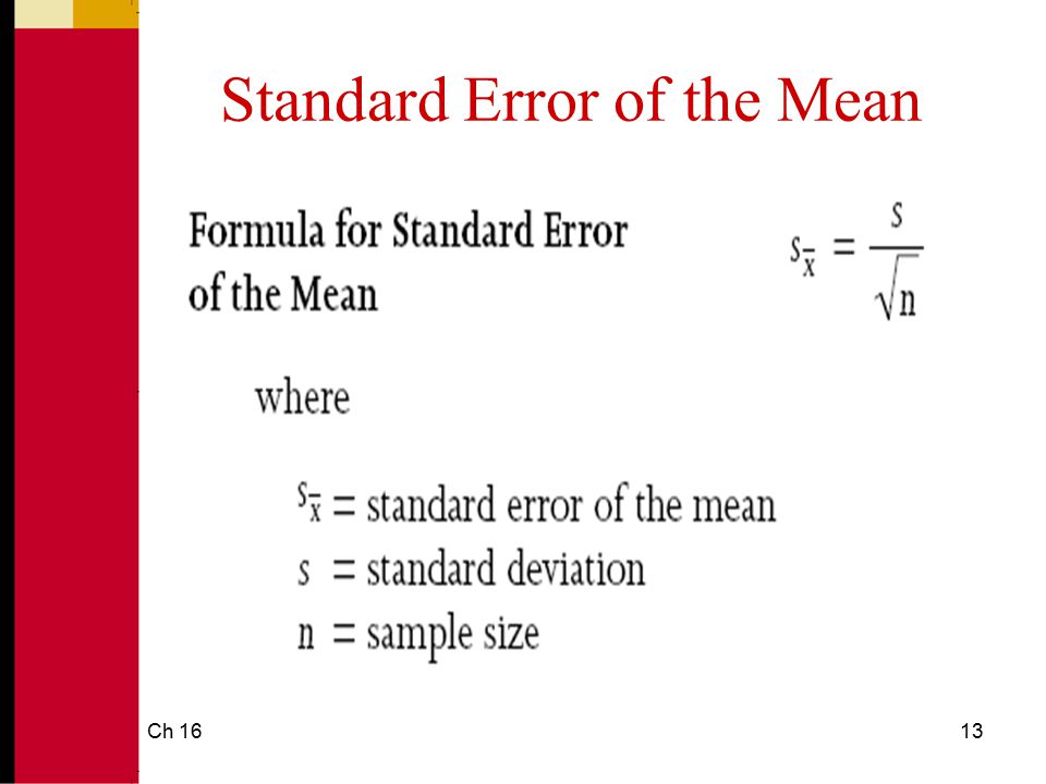
.
The “mean” of a population of measurements does not remove the measurement error. Read the article again and try to understand. For example, take two readings, one 24 deg +- 0.5 and another 30 deg +- 0.5 degrees. The mean is 27 deg but the error term is still +- 0.5 degrees and no amount of averaging will remove that error. So you don’t know the actual temperature inside the range of 27.5 deg to 26.5 deg.
Read Kip’s explanation again. You can calculate the mean out to 10 decimal places but all you’re doing is saying the mean of your calculations is very accurate. That is not the same as saying the mean is an accurate measurement of the temperatures.
I forgot to add, read the link you give very carefully. It says “Standard Error of the Mean”. That is what this article is about. The Error of the Mean may be very small, but it doesn’t mean the accuracy of the measurement have changed.
The only way you can claim the accuracy of the measurements is reduced is to have multiple measurements of THE SAME THING. In other words, line up 100 people to read one, individual thermometer as quickly as they can. Then you may claim the accuracy of the measurement is better by averaging all 100 readings.
If you are concerned with anomalies Jim, you can use my 10 foot stick measurement once, then come back and do the same measurement 5 year later and with as much accuracy as you want, tell if the average height of the population increase, decreased or stayed the same over the five year interval. The difference between the first and the second samples would constitute the “anomaly.”
If you mean the only measurements I can use are 0 feet and 10 feet. There is no way to determine where the actual measurement is therefore the average is meaningless. Sure, you can calculate a mean, but tell everyone what it means.
Even if you use the same people, although they grow , will enough of them do so to make the person taking the measurement round up to 10 feet? Remember, with your device you can only round to 0 feet or 10 feet. In other words, is the temperature 27 degrees or 28 degrees?
Gorman says: “Remember, with your device you can only round to 0 feet or 10 feet.”
..
Please re-read upthread where I posted: ” if you take a stick that is 10 feet tall with markings at one foot intervals”
…
Reading is fundemental
Nick,
Your link appears to be broken.
Thanks, Clyde. The link is here. Actually, it’s a silly reason – I had made a spelling mistake in the original title, echoed in the link. The checker noted it, so I fixed it, and broke the link 🙁
Nick,
Thank you for the corrected link. There is some interesting material there. However, what seems to me to be a glaring error, is not addressing the error of raw measurements. For example, you present the theory of integration and how it can be used to calculate the volume of a sand pile. Like any good mathematician, you assume exact numbers. That is, you ignore the inevitable errors in the real world. In your sand pile case, the apparent depth of the measuring stick may vary by as much as two or three sand grain diameters. Additionally, if the sand is not well-sorted, a large grain on the bottom may keep the stick from getting as close to the bottom as in the other locations sampled. So, you have a mix of known confounding factors (a range of two or three grains where one must make a subjective estimate of the best average), and unknown factors (what is going on at the bottom where it can’t be observed). What you AREN’T doing is providing a rigorous analysis of the errors that modify the results of your theoretical, ideal analysis. In the real world, engineers and scientists don’t have the luxury of idealizing a situation and dealing with only exact numbers.
The engineer can, however, give you a very “accurate and precise” calculation for the number of sand grains in the sandpile.
For a perfect cone of an average pile of average damp sand at an average recline angle of the sand on a perfectly flat surface consisting only of average sized sand grains.
Now for your ACTUAL pile of sand ….. Give me the money and the time, and I WILL count every grain of sand in that pile. And be able to tell you EXACTLY how many grains of sand were in it. But your actual pile of sand may, or may not, have ANY value near the AVERAGE value of that theoretical classroom-lecture pile of sand.
You will then have a data set of 1.
Clyde,
“In the real world, engineers and scientists don’t have the luxury of idealizing a situation…”
Well, the sand might be a place to start talking about the real world. In fact, estimating the volume of a pile of sand is a common real world activity. People buy it by the cubic yard. How is the payment determined? Probably mostly by eye and trust. But a buyer who wanted to check would have to do something pretty much as I described. And he wouldn’t be worrying about a few grains stopping the probe reaching the bottom. And you don’t get to put error bars on your payment.
But in fact I am describing basic calculus, as it goes back to Newton. Engineers do integration too. And they use they theory that I describe.
Nick,
And when you buy sand by the truckload, you don’t need a very accurate or precise estimate of the amount of sand, because you are going to be paying something like $20 per ton at the source, and only have the ability to pay to the nearest penny, assuming that the supplier is going to be worried about a price that precise. What I’m castigating you for is not paying attention to the details of reality, and pretending that everything is exact.
What you should do is calculate the area under the curve for the mean value, and then do the integration with an upper-bound and a lower-bound, as determined by the error in the measurements. You only do the calculation for the mean value, which you treat as being exact.
Repeating what I said above, now updated to use same for anomalies:
These are not repeated measures for the same phenomena, these are singular measures (with ranges) for multiple phenomena (temperature measured at multiple locations).
The reduction in uncertainty by averaging ONLY applies for repeated measures of the (exact) same thing, i.e. the temperature at a single location (at a single point in time).
NOT to the averaging of singular measures for multiple phenomena.
Also measurement error is nice to know, but when small to stddev of sample population it hardly matters. What one does when averaging temperatures across the global is asking what is the typical temperature (on that day).
Say you do that with height of recruits for the army. We use a standard procedure to get good results and a nice measurement tool. Total expected measurement error is say 0.5 cm. We measure 20 recruits (not same recruit 20x).
Here are the results:
recruit # height (in cm, all +/-0.5 cm)
1 182
2 178
3 175
4 183
5 177
6 176
7 168
8 193
9 181
10 187
11 181
12 172
13 180
14 175
15 175
16 167
17 186
18 188
19 193
20 180
Average 179.9
StDev (s) 7.2
95% range
min max
165.5 194.2
Average 179.9 +/-0.5
Min 165.5 +/-0.5
Max 194.2 +/-0.5
Remember that these are different individuals, so not repeated measures of the same thing, but multiple measures of different things, which are then averaged to get an estimate of the midpoint (average) and range (variance).
Both those min, avg and max still also have that measurement error, but we usually forget all about that because it is so small compare to the range of the sample set.
Now we go for a height ‘anomaly’.
Let’s say tha the last 30 years the typical, average height of recruits (at age 18) in county X was : 178.2 (and that had the same measurement error, honest).
Average 179.9 +/-0.5 179.4 179.9 180.4
Min 165.5 +/-0.5 165.0 165.5 166.0
Max 194.2 +/-0.5 193.7 194.2 194.7
base 178.2 +/-0.5 177.7 178.2 178.7
Avg Anomaly 1.7 (0) 1.7 1.7 1.7
Min Anomaly -12.7 (0) -12.7 -12.7 -12.7
Max Anomaly 16.0 (0) 16.0 16.0 16.0
Notice how measurement inaccuracy magically disappears? That’s because I substracted an earlier average (with the same measurement issue) which happens to have the same range. That is just the measurement uncertainty that I make disappear.
But the range within the actual data is very large, and that does not disappear by using anomalies.
The correct anomaly is not 1.7 but is in a 95% range -12.7 to +16.0
Let’s redo the averaging, now with anomaly adjustment before calculating averages and standard deviations:
recruit # height Anomaly
1 3.8
2 -0.2
3 -3.2
4 4.8
5 -1.2
6 -2.2
7 -10.2
8 14.8
9 2.8
10 8.8
11 2.8
12 -6.2
13 1.8
14 -3.2
15 -3.2
16 -11.2
17 7.8
18 9.8
19 14.8
20 1.8
Average 1.7
StDev (s) 7.2
95% range
min max
-12.7 16.0
And the result is exactly the same.
Japp==> Thanks for your long explanation…you just can’t get rid of that original uncertainty ….
+100
“Let’s redo the averaging, now with anomaly adjustment before calculating averages and standard deviations”
Like Kip, you just don’t get the difference between anomaly of mean and mean of anomalies. It makes no difference if you subtract one number from the whole sample. The idea is to subtract estimates that discriminate between the sampled, to take out that aspect of variation which might confound with your sampling process.
To modify your example, suppose they were school cadets, age range 14-18 say. Then the average will depend a lot on the age distribution. That is a big source of sampling uncertainty. But if you calculate an anomaly for each relative to the expected height for that age, variations in age distribution matter a lot less. Then you really do reduce variance.
I’m surprised people just can’t see this distinction, because it is common in handicapping for sport. In golf, you often calculate your score relative to an expected value based on your history. If you want to know whether the club is improving, that “anomaly” is what you should average. We have a Sydney-Hobart yacht race each year. The winner is determined by “anomaly” – ie which did best relative to the expected time for that yacht class. Etc.
Nick ==> A little more honesty wouldn’t be misplaced. In your system you first find medians, then you find averages (means), then you find anomalies of those means from other means, and only then do you find the mean of anomalies.
Kip,
“A little more honesty wouldn’t be misplaced”
More reading, thinking, and less aspersion from you, would be better. There is no measure of medians or interim means in the example here on heights. You simply subtract the age expectation from the measured height.
But if you are referring back to temperature measurement, your assertion is the usual nonsense too. There is no median calculated. It’s true that conventionally the anomaly is formed at the monthly average stage, to save arithmetic operations. But you could equally form daily anomalies, since at that level it is another case of subtracting the same number from each day in the month. So it doesn’t make the slightest arithmetic difference in which order it is done.
Where anomaly makes a difference is in forming the global average for the month. That is when different references (normals) are being subtracted from the different locations in the average. That is when anomaly makes a difference.
Nick ==> The Daily Averages are MEDIANS — read the ASOS User’s Guide, I linked it above. If official Daily Averages are used in your calculations any where, then you have started with Medians. The MONTHLY average, according to the specs, is the MEAN of the Daily Medians.
So — we have, as I stated, first medians, then means of medians, then the Anomaly of Means (Monthly Mean subtracting Climatic Mean), then somewhere up ahead, you take the Mean of Anomalies.
Please correct me if that is not an accurate description of the steps.
I only point it out because of your silly carping about how “Means of Anomalies” is different from “Anomalies of Means”.
In effect and in fact, your method does both.
Kip
“The Daily Averages are MEDIANS”
You just get this stuff wrong in every way. An average of daily min and max is not a median in any sense. A median is an observed vale that is the midway point in order (so it never makes sense to talk of the median of two values). The daily average is not an observed value. But in any case, people often don’t calculate an actual daily average. GHCN publishes an average max for the month, and an average min, and combines those. However, it doesn’t matter in which order you do it.
But you are continually missing the real point of anomalies. They have no useful effect for a station on its own. You can average min and max whenever, add or subtract normals, whatever. Anomalies matter when you combine different locations. They take out the expected component of the variation, which otherwise you would have to treat very carefully to be sure of correct area representation of values.
Nick ==> Did you answer the question on your method for arriving at a Global Average Temperature anomaly? I thought we were talking about whether you do or do not take anomalies of means and/or means of anomalies…..I see that you wish to ignore all the early steps — medians/means of daily Min/Max, and rely on the fact that these statsically dicey parts are auto-magically done by “the GHCN computer”.
So the GHCN — or your software — takes the Mean of Daily Maxes and the Mean of Daily Mins and then takes the Mean (mid-point — the median of a two number set is incidentally the same as the Mean, in all cases) of those two means (we could rightly call this a Mean of Means….) to arrive at what they are then calling the Average Monthly Temperature for the Station?
So, next, are you taking the Anomaly of that Mean of the Means by subtracting the long term Mean of those same Means for a 30-years period? and then the Means of the Anomalies of all the stations to get the Global Mean?
All in all, the system involves Means of Maxes and Means of Mins, then the Median of the two number set (you may call them Means if you wish — both are correct and both the same for a two number set), then the Anomaly of the same hodge-podge for 30 years on the same month (which I point out is a Anomaly of Means), and then aat some distant step later — you take the Mean of the Anomalies — which you will label the Global Average Surface Temperature anomaly.
So, we see here BOTH Anomalies of Means and Means of Anomalies…..correct?
Of course all that finding of Means reduces variability — it is just a form of smoothing.
It does not reduce the uncertainty of the values of the data set — nor of the real world uncertainty surrounding the Global Average Surface Temperature — in any of its forms and permutations.
Kip,
“So the GHCN — or your software — takes the Mean of Daily Maxes and the Mean of Daily Mins and then takes the Mean (mid-point …”
I can’t see where your worrying how the site calculations of monthly average are done at a particular site. The various ways that it could be done will produce essentially the same arithmetic done in different order. But anyway:
My program, TempLS, uses as input GHCN Monthly TAVG, unadjusted (and ERSST V5). That is a published file, as are the monthly averages of max and min (TMAX and TMIN). Most of the older data in GHCN comes from a digitisation (of print or handwriting) program in the early 1990’s. There was very little digitised daily data then; GHCN used printed monthly data from Met Offices etc. Mostly that was recorded as monthly average max and monthly min, which they would average. GHCN Daily, which is a databank of digitised daily, has become substantial only in the last decade.
GHCN still takes in monthly data. It is submitted by Mets on CLIMAT forms, which you cen see eg here. They submit Tx (max), Tn (min) and T (avg). Whether they calculate T as (Tx+Tn)/2 or daily is between them and their computers. It is always true that T=(Tx+Tn)/2 (rounded), but it would be so either way.
Nick,
When there are only two numbers in a list, the median and mean are numerically equal. However, the reason I suggested that median should be used to describe the daily ‘average’ is because it will ALWAYS be half-way between the two extremes. Whereas, in a typical arithmetic mean, it would be unusual for the mean to be in the middle of the list, except for a symmetrical distribution. That is, in the real world of temperatures, I wouldn’t expect the mean of temperatures taken every minute to be half-way between the diurnal high and low. (Maybe over the equatorial oceans at the equinox.)
Clyde and Nick ==> The process for determining the Daily Average [ (Tmax+Tmin)/2 ] calls for arranging the data set in order of magnitude, highest to lowest (or vice versa) and them finding the middle value between the two — if there is no middle value (as in the case every time there are only two values — which is our case) then one calculates (V1 + V2)/2. Since the process involves identifying the highest and lowest values, we know we are finding a median.
Finding an arithmetic mean does not involve any sorting of the data prior to the procedure.
So, Daily Average is a median between the Max and Min for the 24-hour period.
Nick,
You said, “A median is an observed vale that is the midway point in order (so it never makes sense to talk of the median of two values)”
That definition only works for a list with an odd number if items. For all even numbered lists, one still has to find the the midpoint of two numbers. That is, the median.
Clyde,
Yes. The median of 1:9 is 5, but what about 1:10? 5 or 6 or what? You could make an arbitrary choice, ensuring that the median is still a member of the set, or you could split the difference. Fortunately with large disordered sets, there is a good chance that the choice will be between equal values.
Often you use median precisely because it is a member of the set. The median number of children per family might be 2. That might be a more useful figure than saying the mean is 1.7.
But it still doesn’t make sense to talk of the median of two points. It can only be one or the other or the mean. You aren’t adding any meaning.
Nick,
We must live in alternate universes because once again we see things differently. Maybe it is because everything is upside down in Oz. 🙂 The sources I have checked recommend that for lists with an even number of elements, one should interpolate between the two central numbers to determine the median. So, one is ALWAYS dealing with a pair of numbers to calculate the median, for even-numbered lists. A list of just two numbers (T-max, T-min) becomes a degenerate special case that, nevertheless, follows the same rule as all even-numbered lists. You seem to imply that one can only use numbers that actually occur in a list. That isn’t the case with the mean. That is, one does not select the measurement that is closest to the calculated mean. And it isn’t the case with the mode, where one typically has to round off or bin the measurements to insure that a given range of values has elements that occur more than once. The main reason we have these measurements of central tendency is to be able to quantify the skewness of a distribution. With coarse quantization of a measurement, using only actual numbers (+/- 0.5 deg F) calculations of skewness using median will have less accuracy using only actual measured values, versus using the interpolated median (particularly for small sample sizes).
Nick ==>Referring to the currently used Daily Average of the median of the Max and Min is abetter description of both the process and the result — and disambiguates it from what would normally be called a “daliy average” (all values added/number of values).
Nick ==> After some digging around in the GHCN and US daily summaries I have confirmed that your GHCN_Monthly TAVG is in fact the median of the Monthly Mean of Daily Maxes and the Monthly Mean of the Daily Mins.
So you start you whole program with the Median of two Means — a value that does not represent the Average Temperature at the weather station for the month in question in any scientific way at all — and is just an artifact of the sorry state of past weather records — which, unfortunately, can not be made any better.
There is a point in time when records began to be better kept from which sensible daily averages and monthly averages could be calculated — even annual averages.
Instead we continue to use the inadequate, unscientific method which does not reflect the thing we want to know — how much energy is being retained by the climate system as sensible heat? and is that really increasing? decreasing? or staying the same? And, if we have a scientifically defensible answer, how uncertain are we about its value and the value of change?
Nick ==> Regarding your point “But it still doesn’t make sense to talk of the median of two points. It can only be one or the other or the mean. You aren’t adding any meaning.”
We are most certainty adding meaning — at least clarifying meaning. Daily Avg is NOT the average of daily temperatures. But calling it Daily Average implies that it is. Specifically calling it the Median between the Daily Max and the Daily Min makes this clear. A median is a type of average, but we are not taking an average of daily temperature — we are finding the median between the Max and the Min — a different animal altogether.
Nonsense.
Any time you take an average you will also have variance. You can’t get rid of that variance magically.
As I just showed above, it does not matter when you switch to using anomalies, you’ll keep the variance. All you do is that you remove the measurement uncertainty, which is something else.
Does GISS really get daily temperatures by averaging the daily max and min temperature? I suppose this would be okay if the daily temperature distribution was Gaussian. Our newspaper used to publish the hourly temperatures for the previous day. Their distribution was almost never Gaussian. And the lowest temperature was occasionally not at night. I always wondered what be a good representation of the “average” temperature for the day. I don’t think this is a trivial problem. If you can’t get the daily temperature right, how are you going to get the monthly and yearly temperatures right?
old engineer ==> Daily Averages are in fact determined by the Hi+Low/2 method.
Check any station data set.
Kip,
Which fundamentally is the median of two numbers. So, the data processing includes calculating a daily median (and its associated anomaly) followed up by weekly and/or monthly means (which may or may not account for the months having different number of days), and followed up by annual means. Each step applies a low-pass filter, which makes the variance look smaller. The calculated anomalies are used with more significant figures than warranted, and then used to infill over large areas where there is no data. A sorry state of affairs!
Clyde ==> I’ll second that!
Kip,
I should have said the first step is calculating the median of two extremes, without regard to how long the temperatures lasted, and then claiming that we have correctly characterized the average annual temperature.
Clyde ==> Yes, that is exactly how I see it and this is confirmed by the User Guide for the ubiquitous ASOS system, at least for the Daily Station Averages.
GISS doesn’t measure temperatures. But historically, the people who do recorded the daily max and min. It isn’t perfect information, but it isn’t nothing. And it is what we have.
And what we have is bad (and incomplete) data. Bad data leads to bad science.
A true objective scientist would seek the truth, seek good data and good science.
A politically motivated scientist would say “it is what we have” and push forward with their non-scientific agenda driven propaganda.
“…GISS doesn’t measure temperatures…”
He didn’t say they measure anything. He asked if they calculate an average based on min and max.
“It is a trick to cover-up known large uncertainty”
I think that there is a flaw in the use of temperature anomalies in general because the assumed constancy of the seasonal cycle is not found in the data. Please see
https://tambonthongchai.com/2018/08/17/trendprofile/
On the uncertainty issue, Hadcrut4 does include uncertainties. The uncertainty is presented here in graphical form and their impact assessed. But there is something funny about them. Please see
https://tambonthongchai.com/2018/09/17/hadcrut4-uncertainty/
Chaamjamal ==> The actual “uncertainty” they discuss is “THE 95% CONFIDENCE INTERVAL OF UNCERTAINTY.”
It is a statistical animal — it is not the real uncertainty —
Where and when did the use of the word anomaly arise in statistics? As in the first statistics book. The only thing I know of close to precision use is in astronomy, but most use is for an irregular type number, not too confident. Sounds too much like the use of normal for average, which gets drilled (or should) into students as the mean.
The most critical first and important application before you apply all these is (or used to be) care in sampling of attributes. Agree with S. Skinner above but the dictionary definition is different.
Something that I noticed with Australia’s BOM records in recent times. The mean of half hour readings can be a few degrees different to the mean of the highest and lowest values but the official maximum is usually higher of up to two degrees and the mean of the official max and min comes very close to the mean of half hour readings.
If I was more cynical, I would say that this was deliberate.
Temperature is an intensive property but of the probe at any particular time. The mean of the max and min is not. Its not as if its mean of a well spread out sampling. Its the mean of two different times when the thermometer was affected by two very different air masses.
true, but they have also been caught using instantaneous readings instead of 2 minute averages on their electronic gauges, so anything is possible.
Robert ==> You can find these same differences in any complete record of station data. It is not intentional — it is an historic artifact from when temperatures were measured with a Hi/ow (or Max/Min) thermometer — like this one.(at least, the same principle).
So they still figure the Daily Average the same way from the only two values that were recorded in times past.
I checked quite a few years ago how close the mean of the min and max would be to the mean of 24 hours of readings. I was surprised that they were so close considering how much humidity and cloud cover has on the measurements (for an arid area so mins and max tend to vary a lot) and , for the few days that I checked eg. Within a fraction of a degree. I was expecting to show that the mean of the two extreme readings were not anything like an intensive property that a global average of would be meaningful, even if a complete record of evenly spaced measurements. Still bugs me that it was close with the official maximum rather than the highest temp recorded on the published temps eg
http://www.bom.gov.au/products/IDS60801/IDS60801.94648.shtml
The official max was 19.1.
A couple of degrees difference and its clear both are independent indicators of changes but together are meaningless.
Robert B,
Check out some numbers from the NOAA Climate Reference Network.
https://www.ncdc.noaa.gov/crn/qcdatasets.html
Using DAILY data for a particular city and date, look up the DAILY MEAN Temp.
Then look at the SUB-HOURLY data for the same city and same day. Data captured at 5-minute sample rate. Calculate the average for that day (integrate). Compare to the DAILY MEAN.
In the limited examples I have run, I see ~0.4C, 0.7C, 0.9C, 1.0C differences between the 5-minute and daily data.
As I said in another post: the temperature signal is not a purely sinusoidal 1Hz signal. There are higher frequency components. Changes happen over 5 minute spans.
Its is beyond me how climate “science” gets to ignore the Nyquist Sampling Theorem and basically violate it with (Max+Min)/2.
The instrument temperature record is a dumpster fire. Its a monument to how to not be scientific, despite all of the ivory-tower mathematicians deployed in its name.
Does this has any significance with manipulated/adjusted data series.
At individual station level there is a standard procedure to get averages. The same procedure is used to get state averages and country averages. The basic problem here is: they don’t represent the climate system existing in the region or country. Majority of the met stations are located in urban areas. Few stations are located in rural. Also, with passing of time network non-linearly increased and now they are coming down. To over come this problem at regional, country or global level satellite data serve the purpose but unfortunately here also entered the warmist groups to manipulate data. In fact more than a decade back, at a INDIAMET symposium, some groups presented analysis results based on the satellite data released by Ahmedabad group. At the sysmposium, they said the data is not correct. Then I questioned them: why you didn’t tell the users of your data before coming to the conference but no response. Also, there is some other problem: drawing the isolines.
Dr. S. Jeevananda Reddy
Dr. Reddy ==> Your comment is spot on. The Daily Averages of stations do not reflect the climatology of their geographic regions — for many reasons, including station location, UHI effect, and the fact that the “daily averages” are really medians of the Hi/Low.
What the temperature records, up to and including GAST, don’t represent faithfully is whether or not, and if so by how much , the planetary climate system is gaining energy as sensible heat.
Because of the disconnect between recorded temperatures and actual local temperature climatology, the isolines (isotherm lines) will be out of kilter with reality.
Dear Mr. Hansen.
I think there is another, equally important property of measuring instruments that is missing.
That is the property of repeatability. Typically, an instrument will read inaccurately, but they will display the same inaccuracy each time. eg. a NIST traceable instrument that accurately measures to .01C is used to calibrate a mercury thermometer. At 25.00C, the thermometer visually reads between 25 and 25.5C, it is thus within the measurement accuracy of the thermometer. The next time the temperature is brought to 25.00C, the thermometer will still show ~25 1/4C, it would not read 24.5 which is still in the tolerance of the instrument. Thus the temperature is inaccurate, but the inaccuracy is repeatable.
As for trends, if the repeatability of the instrument is high, say .05C, then the trend would have a precision that is 10x more accurate than the actual values. In the Navy, a reading considered accurate of an analog scale would limit precision to 1/2 the value of the graduation increments.
I also do not recall ever seeing signal to noise ratio discussed when it comes to the trend lines and natural variation.
All of that said, when temperature adjustments that are equal to or greater than the anomaly, well, all bets are off. You might as well throw darts.
Jim,
That is assuming that the person reading the thermometer is likewise repeatable. My experience with humans on analog scales is one person can be all over the map reading the exact same reading. It isn’t the instrument which is necessarily picking up the +/-0.5, it is the eyeball reading it. That is even neglecting the days when it is -20 and the person just wants to get his readings and get back into the warmth inside, or it is 102 in the shade and the person wants to get out of the sun and cool off, but has to get this task done. I think +/- 0.5 is probably a little generous in the extremes of summer and winter, but probably about right for the more clement conditions.
Jim G ==> Now days, almost all important stations are using Automated Weather Stations — Automated Surface Observing Systems. Full details at https://www.weather.gov/asos/ with the User’s Guide (really exactly what they do) in a pdf here..
I my opinion, noise to signal ratios apply perfectly fine to radio signals and other messy data. Weather and temperature do not have signal and noise — the record of temperature is simply data — it does not “contain” signal obscured by noise.
Anomalous anomolies anomolize anomolously.
dred ==> Good one!
First the night and day time anomalies are averaged up from which the annual winter and summer anomalies are computed which in turn are averaged from the tropics to the poles to produce a number that we are expected to think actually means something.