Guest Essay by Kip Hansen
 Introduction:
Temperature and Water Level (MSL) are two hot topic measurements being widely bandied about and vast sums of money are being invested in research to determine whether, on a global scale, these physical quantities — Global Average Temperature and Global Mean Sea Level — are changing, and if changing, at what magnitude and at what rate. The Global Averages of these ever-changing, continuous variables are being said to be calculated to extremely precise levels — hundredths of a degree for temperature and millimeters for Global Sea Level — and minute changes on those scales are claimed to be significant and important.
In my recent essays on Tide Gauges, the question of the durability of original measurement uncertainty raised its toothy head in the comments section.
Here is the question I will try to resolve in this essay:
If original measurements are made to an accuracy of +/- X (some value in some units), does the uncertainty of the original measurement devolve on any and all averages – to the mean – of these measurements?
Does taking more measurements to that same degree of accuracy allow one to create more accurate averages or “means”?
My stated position in the essay read as follows:
If each measurement is only accurate to ± 2 cm, then the monthly mean cannot be MORE accurate than that — it must carry the same range of error/uncertainty as the original measurements from which it is made. Averaging does not increase accuracy.
It would be an understatement to say that there was a lot of disagreement from some statisticians and those with classical statistics training.
I will not touch on the subject of precision or the precision of means. There is a good discussion of the subject on the Wiki page: Accuracy and precision .
The subject of concern here is plain vanilla accuracy: “accuracy of a measurement is the degree of closeness of measurement of a quantity to that quantity’s true value.” [ True value means is the actual real world value — not some cognitive construct of it.)
The general statistician’s viewpoint is summarized in this comment:
“The suggestion that the accuracy of the mean sea level at a location is not improved by taking many readings over an extended period is risible, and betrays a fundamental lack of understanding of physical science.”
I will admit that at one time, fresh from university, I agreed with the StatsFolk. That is, until I asked a famous statistician this question and was promptly and thoroughly drummed into submission with a series of homework assignments designed to prove to myself that the idea is incorrect in many cases.
First Example:
Let’s start with a simple example about temperatures. Temperatures, in the USA, are reported and recorded in whole degrees Fahrenheit. (Don’t ask why we don’t use the scientific standard. I don’t know). These whole Fahrenheit degree records are then machine converted into Celsius (centigrade) degrees to one decimal place, such as 15.6 °C.
This means that each and every temperature between, for example, 72.5 and 71.5 °F is recorded as 72 °F. (In practice, one or the other of the precisely .5 readings is excluded and the other rounded up or down). Thus an official report for the temperature at the Battery, NY at 12 noon of “72 °F” means, in the real world, that the temperature, by measurement, was found to lie in the range of 71.5 °F and 72.5 °F — in other words, the recorded figure represents a range 1 degree F wide.
In scientific literature, we might see this in the notation: 72 +/- 0.5 °F. This then is often misunderstood to be some sort of “confidence interval”, “error bar”, or standard deviation.
It is none of those things in this specific example of temperature measurements. It is simply a form of shorthand for the actual measurement procedure which is to represent each 1 degree range of temperature as a single integer — when the real world meaning is “some temperature in the range of 0.5 degrees above or below the integer reported”.
Any difference of the actual temperature, above or below the reported integer is not an error. These deviations are not “random errors” and are not “normally distributed”.
Repeating for emphasis: The integer reported for the temperature at some place/time is shorthand for a degree-wide range of actual temperatures, which though measured to be different, are reported with the same integer. Visually:

Even though the practice is to record only whole integer temperatures, in the real world, temperatures do not change in one-degree steps — 72, 73, 74, 72, 71, etc. Temperature is a continuous variable. Not only is temperature a continuous variable, it is a constantly changing variable. When temperature is measured at 11:00 and at 11:01, one is measuring two different quantities; the measurements are independent of one another. Further, any and all values in the range shown above are equally likely — Nature does not “prefer” temperatures closer to the whole degree integer value.
[ Note: In the U.S., whole degree Fahrenheit values are converted to Celsius values rounded to one decimal place –72°F is converted and also recorded as 22.2°C. Nature does not prefer temperatures closer to tenths of a degree Celsius either. ]
While the current practice is to report an integer to represent the range from integer-plus-half-a-degree to integer-minus-half-a-degree, this practice could have been some other notation just as well. It might have been just report the integer to represent all temperatures from the integer to the next integer, as in 71 to mean “any temperature from 71 to 72” — the current system of using the midpoint integer is better because the integer reported is centered in the range it represents — this practice, however, is easily misunderstood when notated 72 +/- 0.5.
Because temperature is a continuous variable, deviations from the whole integer are not even “deviations” — they are just the portion of the temperature measured in degrees Fahrenheit normally represented by the decimal fraction that would follow the whole degree notation — the “.4999” part of 72.4999°F. These decimal portions are not errors, they are the unreported, unrecorded part of the measurement and because temperature is a continuous variable, must be considered evenly spread across the entire scale — in other words, they are not, not, not “normally distributed random errors”. They only reason they are uncertain is that even when measured, they have not been recorded.
So what happens when we now find the mean of these records, which, remember, are short-hand notations of temperature ranges?
Let’s do a basic, grade-school level experiment to find out…
We will find the mean of a whole three temperatures; we will use these recorded temperatures from my living room:
11:00     71 degrees F

12:00     72 degrees F

13:00     73 degrees F
As discussed above, each of these recorded temperatures really represent any of the infinitely variable intervening temperatures, however I will make this little boxy chart:

Here we see each hour’s temperature represented as the highest value in the range, the midpoint value of the range (the reported integer), and as the lowest value of the range. [ Note: Between each box in a column, we must remember that there are an infinite number of fractional values, we just are not showing them at this time. ] These are then averaged — the mean calculated — left to right: the three hour’s highest values give a mean of 72.5, the midpoint values give a mean of 72, and the lowest values give a mean of 71.5.
The resultant mean could be written in this form: 72 +/- 0.5 which would be a short-hand notation representing the range from 71.5 to 72.5.
The accuracy of the mean, represented in notation as +/- 0.5, is identical to the original measurement accuracy — they both represent a range of possible values.
Note: This uncertainty stems not from the actual instrumental accuracy of the original measurement, which is a different issue and must be considered additive to the accuracy discussed here which arises solely from the fact that measured temperatures are recorded as one-degree ranges with the fractional information discarded and lost forever, leaving us with the uncertainty — a lack of knowledge — of what the actual measurement itself was.
Of course, the 11:00 actual temperature might have been 71.5, the 12:00 actual temperature 72, and the 13:00 temperature 72.5. Or it may have been 70.5, 72, 73.5.
Finding the means kiddy-corner gives us 72 for each corner to corner, and across the midpoints still gives 72.
Any combination of high, mid-, and low, one from each hour, gives a mean that falls between 72.5 and 71.5 — within the range of uncertainty for the mean.

Even for these simplified grids, there are many possible combinations of one value from each column. The means of any of these combinations falls between the values of 72.5 and 71.5.
There are literally an infinite number of potential values between 72.5 and 71.5 (someone correct me if I am wrong, infinity is a tricky subject) as temperature is a continuous variable. All possible values for each hourly temperature are just as likely to occur — thus all possible values, and all possible combinations of one value for each hour, must be considered. Taking any one possible value from each hourly reading column and finding the mean of the three gives the same result — all means have a value between 72.5 and 71.5, which represents a range of the same magnitude as the original measurement’s, a range one degree Fahrenheit wide.
The accuracy of the mean is exactly the same as the accuracy for the original measurement — they are both a 1-degree wide range. It has not been reduced one bit through the averaging process. It cannot be.
Note: For those who prefer a more technical treatment of this topic should read Clyde Spencer’s “The Meaning and Utility of Averages as it Applies to Climate” and my series “The Laws of Averages”.
And Tide Gauge Data?
It is clear that the original measurement accuracy’s uncertainty in the temperature record arises from the procedure of reporting only whole degrees F or degrees C to one decimal place, thus giving us not measurements with a single value, but ranges in their places.
But what about tide gauge data? Isn’t it a single reported value to millimetric precision, thus different from the above example?
The short answer is NO, but I don’t suppose anyone will let me get away with that.
What are the data collected by Tide Gauges in the United States (and similarly in most other developed nations)?

The Estimated Accuracy is shown as +/- 0.02 m (2 cm) for individual measurements and claimed to be +/- 0.005 m (5 mm) for monthly means. When we look at a data record for the Battery, NY tide gauge we see something like this:
| Date Time | Water Level | Sigma |
| 9/8/2017 0:00 | 4.639 | 0.092 |
| 9/8/2017 0:06 | 4.744 | 0.085 |
| 9/8/2017 0:12 | 4.833 | 0.082 |
| 9/8/2017 0:18 | 4.905 | 0.082 |
| 9/8/2017 0:24 | 4.977 | 0.18 |
| 9/8/2017 0:30 | 5.039 | 0.121 |
Notice that, as the spec sheet says, we have a record every six minutes (1/10th hr), water level is reported in meters to the millimeter level (4.639 m) and the “sigma” is given. The six-minute figure is calculated as follows:
“181 one-second water level samples centered on each tenth of an hour are averaged, a three standard deviation outlier rejection test applied, the mean and standard deviation are recalculated and reported along with the number of outliers. (3 minute water level average)”
Just to be sure we would understand this procedure, I emailed CO-OPS support [ @ co-ops.userservices@noaa.gov ]:
To clarify what they mean by accuracy, I asked:
When we say spec’d to the accuracy of +/- 2 cm we specifically mean that each measurement is believed to match the actual instantaneous water level outside the stilling well to be within that +/- 2 cm range.
And received the answer:
That is correct, the accuracy of each 6-minute data value is +/- 0.02m (2cm) of the water level value at that time.
[ Note: In a separate email, it was clarified that “Sigma is the standard deviation, essential the statistical variance, between these (181 1-second) samples.” ]
The question and answer verify that both the individual 1-second measurements and the 6-minute data value represents a range of water level 4 cm wide, 2 cm plus or minus of the value recorded.
This seemingly vague accuracy — each measurement actually a range 4 cm or 1 ½ inches wide — is the result of the mechanical procedure of the measurement apparatus, despite its resolution of 1 millimeter. How so?

NOAA’s illustration of the modern Acoustic water level tide gauge at the Battery, NY shows why this is so. The blow-up circle to the top-left shows clearly what happens at the one second interval of measurement: The instantaneous water level inside the stilling well is different than the instantaneous water level outside the stilling well.
This one-second reading, which is stored in the “primary data collection platform” and later used as part of the 181 readings averaged to get the 6-minute recorded value, will be different from the actual water level outside the stilling well, as illustrated. Sometimes it will be lower than the actual water level, sometimes it will be higher. The apparatus as a whole is designed to limit this difference, in most cases, at the one second time scale, to a range of 2 cm above or below the level inside the stilling well — although some readings will be far outside this range, and will be discarded as “outliers” (the rule is to discard all 3-sigma outliers — of the set of 181 readings — from the set before calculating the mean which is reported as the six-minute record).
We cannot regard each individual measurement as measuring the water level outside the stilling well — they measure the water level inside the stilling well. These inside-the-well measurements are both very accurate and precise — to 1 millimeter. However, each 1-second record is a mechanical approximation of the water level outside the well — the actual water level of the harbor, which is a constantly changing continuous variable — specified to the accuracy range of +/- 2 centimeters. The recorded measurements represent ranges of values. These measurements do not have “errors” (random or otherwise) when they are different than the actual harbor water level. The water level in the harbor or river or bay itself was never actually measured.
The data recorded as “water level” is a derived value – it is not a direct measurement at all. The tide gauge, as a measurement instrument, has been designed so that it will report measurements inside the well that will be reliably within 2 cm, plus or minus, of the actual instantaneous water level outside the well – which is the thing we wish to measure. After taking 181 measurements inside the well, throwing out any data that seems too far off, the remainder of the 181 are averaged and reported as the six-minute recorded value, with the correct accuracy notation of +/- 2 cm — the same accuracy notation as for the individual 1-second measurements.
The recorded value denotes a value range – which must always be properly noted with each value — in the case of water levels from NOAA tide gauges, +/- 2 cm.
NOAA quite correctly makes no claim that the six-second records, which are the means of 181 1-second records, have any greater accuracy than the original individual measurements.
Why then do they make a claim that monthly means are then accurate to +/- 0.005 meters (5 mm)? In those calculations, the original measurement accuracy is simply ignored altogether, and only the reported/recorded six-minute mean values are considered (confirmed by the author) — the same error that is made as with almost all other large data set calculations, applying the inapplicable Law of Large Numbers.
Accuracy, however, as demonstrated here, is determined by the accuracy of the original measurements when measuring a non-static, ever-changing, continuously variable quantity and which is then recorded as a range of possible values — the range of accuracy specified for the measurement system — and cannot be improved when (or by) calculating means.
Take Home Messages:
- When numerical values are ranges, rather than true discrete values, the width of the range of the original value (measurement in our cases) determines the width of the range of any subsequent mean or average of these numerical values.
- Temperatures calculated from ASOS stations however are recorded and reported temperatures as ranges 1°F wide (0.55°C), and such temperatures are correctly recorded as “Integer +/- 0.5°F”. The means of these recorded temperatures cannot be more accurate than the original measurements –because the original measurement records themselves are ranges, the means must be denoted with the same +/- 0.5°F.
- The same is true of Tide Gauge data as currently collected and recorded. The primary record of 6-minute-values, though recorded to millimetric precision, are also ranges with an original accuracy of +/- 2 centimeters. This is the result of the measurement instrument design and specification, which is that of a sort-of mechanical averaging system. The means of tide gauge recorded values cannot be made more accurate the +/- 2 cm — which is far more accurate than needed for measuring tides and determining safe water levels for ships and boats.
- When original measurements are ranges, their means are also ranges of the same magnitude. This fact must not be ignored or discounted; doing so creates a false sense of the accuracy of our numerical knowledge. Often the mathematical precision of a calculated mean overshadows its real world, far fuzzier accuracy, leading to incorrect significance being given to changes of very small magnitude in those over-confident means.
# # # # #
Author’s Comment Policy:
Thanks for reading — I know that this will be a difficult concept for some. For those, I advise working through the example themselves. Use as many measurements as you have patience for. Work out all the possible means of all the possible values of the measurements, within the ranges of those original measurements, then report the range of the means found.
I’d be glad to answer your questions on the subject, as long as they are civil and constructive.
# # # # #
Thank you for all the hard work.
The first place to start is to point out that Global Average Temperature is NOT a “physical quantity”. You can not take the average of temperature, especially across vastly different media like land sea and ice. It’s scientific bullshit.
Are land + sea temperature averages meaningful?
https://judithcurry.com/2016/02/10/are-land-sea-temperature-averages-meaningful/
Before you start arguing about uncertainty ( which is a very good argument to get into ) you need to make sure are measuring something that is physically meaningful.
Greg, if you don’t think there is a physical “global temperature” what is your opinion of the global average of temperature anomalies? Ditto for sea surface levels.
This whole subject of uncertainty and measurement error is very complex out side a carefully constructed lab experiment. It is certainly key to the whole climate discussion and is something that Judith Curry has been pointing out fro at least a decade now.
However, this simplistic article by Kip does not really advance the discussion and sadly is unlikely to get advanced very much an anarchic chain of blog posts.
Kip clearly does not have the expertise to present a thorough discussion. It would be good if someone like his stats expert could have would have written it. This definately does need a thorough treatment and the currently claimed uncertainties are farcical, I will second him on that point.
Greg. You won’t get any argument from me that “Global Average Temperature” isn’t a poor metric. It’s very sensitive to the constantly changing distribution of warm water in the Pacific Ocean basin. Why would anyone not working on ENSO want a temperature metric that behaves like that? But it really is a physical quantity — if an inappropriate one for the purposes it’s being used for. Don’t you think it was almost certainly lower at the height of the last glaciation, or higher during the Cretaceous?
“if you don’t think there is a physical “global temperature”” – It’s not an opinion. It stems from the definition of temperature. They do indeed extend the notion of temperature in some very special cases for systems out of thermodynamic equilibrium, but typically it’s for dynamical equilibrium and they do lead to nonsense when taking out of context (such as absolute negative temperature). But for systems that are not even in dynamical equilibrium, such as Earth, it’s pure nonsense to average an intensive value that can be defined only locally, due of cvasiequilibrium. It’s not only pure nonsense, but it’s very provable that if you still insist of using such nonsense, you’ll get the wrong physical results out of calculation, even for extremely simple systems.
Don , maybe you should read the link in my first comment. There is a whole article explaining why global mean temperature is not physically meaningful.
Greg ==> I don’t disagree about global means — but one has to call them something — they certainty are a hot topic of conversation and research, even if they don;t really exist.
Dr. Curry’s point are well taken, many people do not understand the differences between energy and temperature. I also point out that “average daily temperature,” which has been interpreted as the average of the daily maximum and minimum is also misunderstood. We are now able to take temperature at the interval of our choice and come up with a weighted average. The average computed from just one daily maximum and one daily minimum assumes the temperatures spend equal amount of time clustered around the average. This is clearly not the case. So when comparing historical temperatures to newer values, it is important to realize the differences.
just to be clear oeman50, that was my article that Judith Curry published on here site. Note the credit just below the title. 😉
The main problem with averaging anything globally is that no living thing on Earth actually experiences the global average. Additionally, the average temperature tells us nothing about the daily range of temperatures. If I experience a day which is 60 degrees in the morning, and 100 degrees in the afternoon, is it not hotter than a day which starts out at 75 and reaches a high of 95? Yet once averaged, the 95 degree day is reported as 5 degrees hotter than the 100 degree day. Of course it gets more complex, but it would be like calculating a globally averaged per capita crime rate. You could do it, but it would be a useless number because the only thing that is important is the criime rate where you are or plan to be. Same with temperature. If we experience a decade where the global average temperature goes up a small amount, was it higher daytime highs that caused it? Was it higher daytime lows that caused it? Was the range the same, but the heat lingered on a little longer after sunset? You can’t tell what is happening unless you look at local specifics, hour by hour. It would be like trying to tell me what song I’m thinking of if I just told you what the average musical note was. Meaning is in the details.
In the same vein, I’ve always wondered why we track the CO2 content of the atmosphere without tracking all of the other greenhouse gases as closely. If CO2 concentration goes up, do we know for a fact that that increases the total amount of greenhouse gases? Could another gas like water vapor decrease at times to balance out or even diminish the total?
It just seems to me that we are standing so far back trying to get the “big picture” that we are missing the details that would have told us the picture was a forgery.
I’m no scientist, so blast me if I’m wrong, but the logic of it all seems to be lost.
Which is why only satellite, radiosonde and atmospheric reanalysis information [I hesitate to use “data.”] are appropriate for use in determining any averages, trends, etc.
In a few [number of?] years ARGO may be useful. Early ARGO information shows no worrisome patterns.
@ur momisugly Greg “This whole subject of uncertainty and measurement error is very complex”
Yes it is: “In 1977, recognizing the lack of international consensus on the expression of uncertainty in measurement, the world’s highest authority in metrology, the Comité International des Poids et Mesures (CIPM), requested the Bureau International des Poids et Mesures (BIPM) to address the problem in conjunction with the national standards laboratories and to make a recommendation.”
It took 18 years before the first version of a standard that deals with these issues in a successful way, was finally published. That standard is called: ´Guide to the expression of uncertainty in measurement´. There now exists only this one international standard for expression of uncertainty in measurement.
“The following seven organizations supported the development of the Guide to expression of uncertainty, which is published in their name:
BIPM: Bureau International des Poids et Measures
IEC: International Electrotechnical Commission
IFCC: International Federation of Clinical Chemistry
ISO: International Organization for Standardization
IUPAC: International Union of Pure and Applied Chemistry
IUPAP: International Union of Pure and Applied Physics
OlML: International Organization of Legal Metrology ..”
The standard is freely available. I think of it as a really good idea to use that standard for what should be obvious reasons. Even some climate scientists are now starting to realize that international standards should be used. See:
Uncertainty information in climate data records from Earth observation:
“The terms “error” and “uncertainty” are often unhelpfully conflated. Usage should follow international standards from metrology (the science of measurement), which bring clarity to thinking about and communicating uncertainty information.”
“Before you start arguing about uncertainty ( which is a very good argument to get into ) you need to make sure are measuring something that is physically meaningful.”
They are connected. The mean of an infinite number of measurements should give you the true value if individual measurements were only off due to random error. You need precise measurements to be sure that the distribution is perfect if you want others to believe that 10 000 measurements has reduced the error by √100. Even the act of rounding up or down means that you shouldn’t pretend that the errors were close to a symmetrical distribution and definitely not close enough to attribute meaning to a difference of 1/100th of the resolution. How anyone could argue against it is beyond me.
To then do it for something that it not an intrinsic property is getting silly. I know what people are thinking but the air around a station in the morning is not the same as that around it when the max is read.
Agreed, TG!
An excellent essay Kip!
I worked with IMD in Pune/India [prepared formats to transfer data on to punched cards as there was no computer to transfer the data directly]. There are two factors that affect the accuracy of data, namely:
Prior to 1957 the unit of measurement was rainfall in inches and temperature in oF and from 1957 they are in mm and oC. Now, all these were converted in to mm and oC for global comparison.
The second is correcting to first place of decimal while averaging: 34.15 is 34.1; 34.16 is 34.2; 34.14 is 34.1 and 34.25 is 34.3; 34.26 is 34.3; 34.24 is 34.2
Observational error: Error in inches is higher than mm and Error in oC is higher than oF
These are common to all nations defined by WMO
Dr. S. Jeevananda Reddy
Dr. Reddy, Very interesting. By the way, you can use alt-248 to do the degree symbol, °.
Take care,
Thank you for this information. I have always suspected the reported accuracy of many averaged numbers were simply impossible. This helps to clarify my suspicions. I also do not understand how using 100 year old measurements mixed with modern ones can result in the high accuracy stated in many posts. They seem to just assume that a lot of values increases the final accuracy regardless of the origin and magnitude of the underlying uncertainties.
Only bullshit results. Even for modern measurements, it’s the hasty generalization fallacy to claim that it applies to the whole Earth. Statisticians call it a convenience sampling. And that is only for the pseudo-measurement that does not evolve radically over time. Combining all together is like comparing apples with pears to infer things about a coniferous forest.
Standard calculations in Chemistry carefully watch the significant digits. 5 grams per 7 mililiters is reported as 0.7 g/mL. Measuring several times with such low precision results in an answer with equally low precision. The extra digits spit out by calculators are fanciful in the real world.
People assume that modern digital instruments are inherently more accurate than old-style types. In the case of temperature at least this is not necessarily so. When temperature readings are collated and processed by software yet another confounding factor is introduced.
With no recognition of humidity, differing and changing elevation, partial sampling and other data quality issues, the idea that we could be contemplating turning the world’s function inside out over a possible few hundredths of a degree in 60 years of the assumed process is plainly idiotic.
AGW is an eco Socialist ghost story designed to destroy Capitalism and give power to those who can’t count and don’t want to work. I’m hardly a big fan of Capitalism myself but I don’t see anything better around. Socialism has failed everywhere it’s been tried.
If quantization does not deceive you Nyqust will.
Kip says: “If each measurement is only accurate to ± 2 cm, then the monthly mean cannot be MORE accurate than that — it must carry the same range of error/uncertainty as the original measurements from which it is made. Averaging does not increase accuracy.”
…
WRONG!
…
the +/- 2cm is the standard deviation of the measurement. This value is “sigma of x ” in the equation for the standard error of the estimator of the mean:
https://www.bing.com/images/search?view=detailV2&ccid=CYUOXtuv&id=B531D5E2BA00E15F611F3DAEC1B85110014F74C6&thid=OIP.CYUOXtuvcFogpL3jEnQw_gEsBg&q=standard+error&simid=608028072239301597&selectedIndex=1
…
The error bars for the mean estimator depends on the sqrt of “N”
roflmao..
You haven’t understood a single bit of what was presented, have you johnson
You have ZERO comprehension when that rule can and can’t be used, do you. !!
(Andy, you need to do better than this when you think Johnson or anyone else is wrong. Everyone here is expected to moderate themselves according to the BOARD rules of conduct. No matter if Johnson is right or wrong,being rude and confrontative without a counterargument,is not going to help you) MOD
I know perfectly well when to use standard error for the estimator of the mean.
…
See comment by Nick Stokes below.
Andy, how about you drop the aggressive, insulting habit of addressing all you replies to “johnson”. If you don’t agree with him, make you point. Being disrespectful does not give more weight to your point of view.
Also getting stroppy from the safely of your keyboard is a bit pathetic.
lighten up greg
ROFL^2
You are a bit rude, Andy, but you are right.
Can we all TRY to be both polite and scientifically /mathematically correct please. It makes for a better blog all round.
Is Andy any ruder than Johnson was?
Especially when Johnson ignores facts, documentation and evidence presented in order to proclaim his personal bad statistics superior.
Nor should one overlook Johnson’s thread bombings in other comment threads.
Sorry, but it very obvious that mark DID NOT understand the original post.
When their baseless religion relies totally on a shoddy understand of mathematical principles, is it any wonder the AGW apostles will continue to dig deeper?
“I know perfectly well when to use standard error for the estimator of the mean.”
Again. it is obvious that you don’t !!
For those who are actually able to comprehend.
Set up a spreadsheet and make a column as long as you like of uniformly distributed numbers between 0 and 1, use =rand(1)
Now calculate the mean and standard deviation.
The mean should obviously get close to 0.5..
but watch what happens to the deviation as you make “n” larger.
For uniformly distributed numbers, the standard deviation is actually INDEPENDENT of “n”
darn typo..
formula is ” =rand()” without the 1, getting my computer languages mixed up again. !!
Furthermore, since ALL temperature measurements are uniformly distributed within the individual ranged used for each measurement, they can all be converted to a uniform distribution between 0 and 1 and the standard deviation remains INDEPENDENT OF “n”</strong)
Obviously, that means that the standard error is also INDEPENDENT of n
Andy, standard deviation and sampling error are not the same things, so please tell me what you think your example is showing?
Sorry you are having problems understanding, Mark.. Your problem, not mine.
Another simple explanation for those with stuck and confused minds.
Suppose you had a 1m diameter target, and, ignoring missed shots”, they were random uniformly distributed on the target.
Now, the more shots you have, the closer the mean will be to bulls eye..
But the error from that mean with ALWAYS be approximately +/- 0.5m uniformly distributed.
“The mean should obviously get close to 0.5.”
“Obviously, that means that the standard error is also INDEPENDENT of n”
Those statements are contradictory. Standard error is the error of the mean (which is what we are talking about). If it’s getting closer to 0.5 (true) then the error isn’t independent of n. In fact it is about sqrt(1/12/n).
I did that test with R : for(i in 1:10)g[i]=mean(runif(1000))
The numbers g were
0.5002 0.5028 0.4956 0.4975 0.4824 0.5000 0.4865 0.5103 0.5106 0.5063
Standard dev of those means is 0.00930. Theoretical is sqrt(1/12000)=0.00913
Seems to me that no matter how data is treated or manipulated there is nothing that can be done to it which will remove the underlying inaccuracies of the original measurements.
If the original measurements are +/- 2cm then anything resulting from averaging or mean is still bound by that +/- 2cm.
Mark, could you explain why you believe that averagaing or the mean is able to remove the original uncertainty ? because I can’t see how it can.
Btw I can see how a trend might be developed from data with a long enough time series – But until the Trend is greater than the uncertainty it cannot constitute a valid trend.
e.g. In temperature a trend showing an increase of 1 deg C from measurements with a +/- 0.5 deg C (i.e. 1 deg C spread) cannot be treated as a valid trend until it is well beyond the 1 deg C, and even then it remains questionable.
I’m no mathematician or statistician but to me that is plain commonsense despite the hard-wired predilection for humans to see trends in everything ………
Maybe someone here has experience with information theory, I did some work with this years ago in relation to colour TV transmissions and it is highly relevant to digital TV . All about resolution and what you need to start with to get a final result. I am quire rusty on it now but think it is very relevant here, inability to get out more than you start with.
Old England:
Consider this; you take your temperature several times a day for a period of time.
Emulating NOAA, use a variety of devices from mercury thermometers, alcohol thermometers, cheap digital thermistors and infra red readers.
Sum various averages from your collection of temperatures. e.g.;
Morning temperature,
Noon temperature,
Evening temperature,
Weekly temperature,
Monthly temperature,
Lunar cycle temperatures, etc.
Don’t forget to calculate anomalies from each average set. With such a large set of temperatures you’ll be able to achieve several decimal places of precision, though of very dubious accuracy.
Now when your temperature anomaly declines are you suffering hypothermia?
When your temperature anomaly is stable are you healthy?
When your temperature anomaly increases, are you running a fever or developing hyperthermia?
Then after all that work, does calculating daily temperatures and anomalies to several decimal places really convey more information than your original measurement’s level of precision?
Then consider; what levels of precision one pretends are possible within a defined database are unlikely to be repeatable for future collections of data.
i.e. a brief window of data in a cycle is unlikely to convey the possibilities over the entire cycle.
Nor do the alleged multiple decimals of precision ever truly improve the accuracy of the original half/whole degree temperature reading.
Then, consider the accuracy of the various devices used; NOAA ignores error rates inherent from equipment, readings, handlings, adjustments and calculations.
“The error bars for the mean estimator depends on the sqrt of “N””
Only true if the measured quantity consists of independent and identically distributed random variables. Amazing how few people seem to be aware of this.
Good luck in proving that there is no autocorrelation between sea-level measurements Mark!
Mark ==> You present exactly what I point out is the misunderstanding when a tide gauge measurement is presented as an integer — notated as 100 +/- 2cm. The +/-2cm is NOT a standard deviation, not an error bar, not a confidence interval — but it sure looks like one as they are all written in the same way. In actual fact, it is the uncertainty of the measurement, brought about by the physical design of the measurement instrument.
Kip: ” In actual fact, it is the uncertainty of the measurement ”
..
Maybe this can clear up your misunderstanding: https://explorable.com/measurement-of-uncertainty-standard-deviation
….
Just remember std deviation is defined independent of the underlying distribution…(i.e. normal, uniform, geometic, etc.)
“The +/-2cm is NOT a standard deviation, not an error bar, not a confidence interval”
Then what is “uncertainty”?
Kip/Nick: Actually a stated instrument MU is a confidence interval. It is defined in the ISO Guides and elsewhere (including NIST) as:
The default is a 95% confidence interval. Thus a measured value of 100 cm can be said to have a true value of between 98 and 102 cm with a 95% confidence if the instrument MU is +/- 2 cm. While it is indeed derived from the standard deviations of various factors that affect the measurement, it is actually a multiple of the combined SDs. Two times the SD for a 95% MU confidence. However, it is not related to the SD of multiple measurements of the measurand. This is a measure of the variability of the thing being measured and such variability is only partly the result of instrument MU. Proper choice of instruments should make instrument MU a negligible issue. Problems arise when the measurement precision required to make a valid determination is not possible with the equipment available. In short, if you want to measure sea level to +/- 1 mm you need a measuring device with an MU of less than 1 mm.
Put another way, you can’t determine the weight of a truck to the nearest pound by weighing it on a scale with a 10 pound resolution no matter how many times you weigh it.
Above I referred to multiple sources of MU that need to be combined. This is known as an uncertainty budget. As an example a simple screw thread micrometer includes the following items: repeatability, scale error, zero point error, parallelism of anvils, temperature of micrometer, temperature difference between micrometer and measured item. However, the vast majority of instrument calibrations are done by simple multiple comparisons of measured values of certified reference standards. In these calibrations there are always at least three sources of MU. The uncertainty of the reference standard, one half the instrument resolution and the standard deviation of the repeated comparison deviation from the reference value. In addition, to be considered adequate the Test Uncertainty Ratio (MU of device being calibrated divided by MU of reference) must be at least 4:1.
This is all basic metrology that should be well understood by any scientist or engineer. But I know from experience that it is not as is clearly evident in these discussions.
Thanks again for you clear and well informed opinion on these matters.
The problem with using S.D as the basis for establishing “confidence intervals” is that it is based soley on statistics and addresses only the sampling error.
If global mean SST is given as +/-0.1 deg C then a “correction” is made due to a perceived bias of 0.05 deg and the error bars are the same ( because the stats are still the same ) then we realise that they are not including all sources of error and the earlier claimed accuracy was not correct.
The various iterations of hadSST have not changed notably in their claimed confidence levels yet at one point they introduced -0.5 deg step change “correction”. This was later backed out and reintroduced as a progressive change, having come up with another logic to do just about the same overall change of 0.5 deg C.
Variance derived confidence levels do NOT reflect the full range of uncertainty, only one aspect: sampling error.
Greg ==> Best stay clear of the Statistics Department at the local Uni….they don’t like that kind of talk. Here either…as you see.
Mark S, you missed the whole point of why this isn’t so in the case of temperatures and tide gauges. If you measure the length of a board a dozen times carefully, then you are right. But if the board keeps changing its own length, then multiple measurings are not going to prove more accurate or even representative of anything. I hope this helps.
If the measurement is made of the same thing, the different results can be averaged to improve the accuracy.
Since the temperature measurements are being made at different times, they cannot be used to improve the accuracy.
That’s basic statistics.
Measuring an individual “thing” and sampling a population for an average are two distinct, and different things. You seem to be confusing the two.
Mark S Johnson,
You are quite wrong. If I handed you an instrument I calibrated to some specific accuracy, say plus or minus one percent of full scale for discussion purposes, you had better not claim any measurement made with it, or any averages of those values, is more accurate than what I specified. In fact, if the measurement involved safety of life, you must return the instrument for a calibration check to verify it is still in spec.
Where anyone would come up with the idea that an instrument calibration sticker that say something like “+/- 2 cm” indicates a standard deviation, I cannot imagine. In the cal lab, there is no standard deviation scheme for specifying accuracy. When we wrote something like “+/- 2 cm”, we meant that exactly. That was the sum of the specified accuracy of the National Bureau of Standards standard plus the additional error introduced by the transfer reference used to calibrate the calibration instrument plus the additional error introduced by the calibration instrument used on your test instrument.
Again, that calibration sticker does not say “+/- 2 cm” is some calculated standard deviation from true physical values. It means what at each calibration mark on the scale, the value will be within “+/- 2 cm” of true physical value. That does not, however specify the Precision of the values you read. That is determined by the way the instrument presents its values. An instrument calibrated to “+/- 2 cm” could actually have markings at 1 cm intervals. In that case, the best that can be claimed for the indication is +/- 0.5 cm. The claimed value would then be +/- 0.5 cm plus the +/- 2 cm calibration accuracy. Claiming an accuracy of better than +/- 2.5 cm would in fact be wrong, and in some industries illegal. (Nuclear industry for example.)
So drop the claims about standard deviation in instrument errors. It does not even apply to using multiple instrument reading the same process value at the same time. In absolutely no case can instrument reading values be assumed to be randomly scattered around true physical values within specified instrument calibration accuracy. Presenting theories about using multiple instruments from multiple manufacturers, each calibrated with different calibration standards by different technicians or some such similar example is just plain silly when talking about real world instrumentation use. You are jumping into the “How many angels can dance on the head of a pin” kind of argument.
Gary, they do not make an instrument that can measure “global temperature.”
…
Measuring “global temperature” is a problem in sampling a population for the population mean. Once you understand this, you may be able to grasp the concept of “standard error” which is comprised of the standard deviation of the instrument used for measurement, divided by the sqrt of the number of obs.
…
Now when/if they build an instrument that can measure the global temperature with one reading, then your argument might hold water.
Mark,
Where above do I mention “global temperature”? My statements were about the use of instrument readings (or observations to the scientific folks.) I would suggest that however that “global temperature” be derived, it cannot claim an accuracy better than the calibration accuracy of the instrumentation used. Wishful thinking and statistical averaging cannot change that.
Remember the early example of averages of large numbers was based upon farm folks at an agricultural fair guessing the weight of a bull. The more guesses that were accumulated, the closer the average came to the true weight. Somehow that has justified the use of averaging in many inappropriate situations. Mathematical proofs using random numbers do not justify or indicate the associated algorithms are universally applicable to real world situations.
Gary, the estimator of the population mean can be made more accurate with more observations. The standard error is inversely proportional to the sqrt of the number of obs.
…..
Here’s an example.
….
Suppose you wanted to measure the average daily high temperature for where you live on Oct 20th. You measure the temp on Oct 20th next Friday.
…
Is this measure any good?
…
Now, suppose you do the same measurement 10/20/2017, 10/20/2018, 10/20/2019 and 10/20/2020, then take the average of the four readings.
..
Which is more accurate?…..the single lone observation you make on Friday, or the average of the four readings you make over the next four years?
….
If you are interested in the real climatic average for your location on Oct 20th, you really need 30 years of data to be precise.
Gary, RE: weight of bull.
…
Here you go again with an incorrect analogy. The weight of an individual bull is not a population mean. Don’t confuse the two. The correct “bull” analogy would be to actually measure the weight of 100 bulls, to determine what the average weight of a bull is. The more bulls you measure, the closer you will get to what the “real” average bull weight is.
BZ!
There will be some of us (like Gary and myself) on here who have regularly sent instruments away to be calibrated and had to carefully consider the results, check the certificates etc. We appear to know rather more about this than some contributors today. I find it interesting that a simple experience like this can help a lot in an important discussion.
“the estimator of the population mean can be made more accurate with more observations. The standard error is inversely proportional to the sqrt of the number of obs.”
Two points here: 1. “estimator” mean guess. 2. your estimator may be made more precise according to a specified estimation algorithm. That does not relate to its accuracy. Your comment about standard deviation only applies to how you derive your guess.
“If you are interested in the real climatic average for your location on Oct 20th, you really need 30 years of data to be precise.”
Good now we are on the same page. You are achieving a desired PRECISION. Accuracy, however remains no better than the original instrumentation accuracy and often worse depending upon how the data is mangled to fit your algorithm. (F to C etc.)
“Here you go again with an incorrect analogy. The weight of an individual bull is not a population mean. Don’t confuse the two. The correct “bull” analogy would be to actually measure the weight of 100 bulls, to determine what the average weight of a bull is. The more bulls you measure, the closer you will get to what the “real” average bull weight is.”
Nope, the exercise was to determine the accuracy of guesses about the weight of a single bull tethered to a post at the fair. A prize was awarded to the person who guessed the closest. It was not about guessing the weight bulls as a population. The observation about that large numbers of guesses was that the average became closer to true weight of the bull as the number of guess increased, one guess per person. It was never claimed that random guess about random bulls would average to any meaningful or useful number.
Guessing the weight of an individual bull is not the same as sampling a population. Hey…..ever hear about destructive testing? It’s what happens when running the test obliterates the item “measured.” For example, how would you insure the quality of 1000 sticks of dynamite? Would you test each one, or would you take a representative random sample and test the smaller number?
Mark S Johnson October 15, 2017 at 9:02 am
“The weight of an individual bull is not a population mean. Don’t confuse the two.”
He didn’t confuse anything. He said “The more guesses that were accumulated, the closer the average came to the true weight. Somehow that has justified the use of averaging in many inappropriate situations.” But you like to fly off on your own illogical tangent, which just gets in the way of those of us trying to understand the arguments.
Then explain how that applies if the measurements are not normally distributed? And if you have no idea if they are normally distributed?Let’s say the sides of the block of metal I have on my desk.
Just to clarify Andy’s concerns. Mark Johnson is confusing uncertainty of the estimate with accuracy of the measure; they’re two different things, something Kip attempts to point out in his essay and also something that anyone familiar with measurement theory and statistics would understand from his essay. It’s possible a person without much practical experience in numerical modeling might miss the distinction, but I can assure you it’s there.
While the “law of large numbers” will reduce the error of estimate as Mark describes, it does nothing to increase accuracy of the measure.
Maybe another example is in order?
If a single measure is accurate +/- 2cm, it has an uncertainty associated with it also, which may perhaps be +/- 5mm. As repeated measures are taken and averaged, the uncertainty (5mm) can be reduced arithmetically as Mark Johnson describes, but the result is a measure accurate +/- 2cm with a lower uncertainty (for example +/- .1 mm).
I hope that resolves the conflicting views expressed here. I agree there’s no reason for ad hominem by either party. It’s a very confusing subject for most people, even some who’ve been involved with it professionally.
When what you are measuring is a population mean, it most certainly does increase the accuracy.
Mark S Johnson: The only person on this thread discussing measures of a population mean is you, and it’s almost certain the only training in statistics you’ve ever had involved SPSS.
Error in a measure is assumed to be normally distributed, not the measure itself. You need to meditate on that. The accuracy of a measure has nothing to do with the uncertainty of the estimate. The “law of large numbers” doesn’t improve accuracy, it improves precision. You’re wrong to argue otherwise.
Bartleby,
That is particularly true if there is a systematic error in the accuracy. If you have a roomful of instruments, all out of calibration because over time they have drifted in the same direction, using them to try to obtain an average will, at best, give you an estimate of what the average error is, but it will not eliminate the error. The only way that you are going to get the true value of the thing you are measuring is to use a high-precision, well-calibrated instrument.
Certainly true if there is systemic error, which really means the measure is somehow biased (part of an abnormal distribution); unless the error of estimate is normal, the law of large numbers can’t be used at all. It can never be used to increase accuracy.
The whole idea of averaging multiple measures of the same thing to improve precision is based on something we call a “normal error distribution” as you point out. We assume the instrument is true within the stated accuracy, but that each individual observation may include some additional error, and that error is normally distributed.
So, by repeatedly measuring and averaging the result, the error (which is assumed normal) can be arithmetically reduced, increasing the precision of the estimate by a factor defined by the number of measures. This is the “Students T” model.
But accuracy isn’t increased, only precision. 100 measures using a device accurate +/- 2cm will result in a more precise estimate that’s accurate to +/- 2cm.
Accuracy and Precision are two very different things.
‘The whole idea of averaging multiple measures of the same thing to improve precision is based on something we call a “normal error distribution”…’
Normal (or Gaussian) distributions are not required, though a great many measurement error sets do tend to a Normal distribution due to the Central Limit Theorem.
All that is required is that the error be equally distributed in + and – directions. Averaging them all together then means they will tend to cancel one another out, and the result will, indeed, be more accurate. Accuracy means that the estimate is closer to the truth. Precision means… well, a picture is worth a thousand words. These arrows are precise:

Bartemis illustrates very effectively, the difference between accuracy and precision.
Bartleby,
“100 measures using a device accurate +/- 2cm will result in a more precise estimate that’s accurate to +/- 2cm.
Accuracy and Precision are two very different things.”
Yes, if you are talking about a metrology problem, which is the wrong problem here. No-one has ever shown where someone in climate is making 100 measures of the same thing with a device. But there is one big difference between accuracy and precision, which is in the BIPM vocabulary of metrology, much cited here, but apparently not read. It says, Sec 2.13 (their bold):
“NOTE 1 The concept ‘measurement accuracy’ is not a quantity and is not given a numerical quantity value. “
Which makes sense. Accuracy is the difference between the measue and the true value. If you knew the true value, you wouldn’t be worrying about measurement accuracy. So that is the difference. If it has numbers, it isn’t accuracy.
Nick Stokes (perhaps tongue in cheek) writes: “So that is the difference. If it has numbers, it isn’t accuracy.”
Nick, if it doesn’t have numbers, it isn’t science. 🙂
Bartleby,
“isn’t science”
Well, it’s in the BIPM vocabulary of metrology.
Nick, there’s an old, old saying in the sciences that goes like this:
If you didn’t measure it, it didn’t happen.”
I sincerely believe that. So any “discipline” that spurns “numbers” isn’t a science. QED.
Bartleby,
I’m not the local enthusiast for use of metrology (or BIPM) here. I simply point out what they say about the “concept ‘measurement accuracy’”.
Nick Stokes writes: “I’m not the local enthusiast for use of metrology (or BIPM) here. I simply point out what they say about the “concept ‘measurement accuracy’”
OK. I don’t think that changes my assertion, that science is measurement based and so requires the use of numbers.
I’m not sure if you’re trying to make an argument from authority here? Id so it really doesn’t matter what the “BIPM” defines; accuracy is a numerical concept and it requires use of numbers. There’s no alternative.
If, in the terms of “metrology”, numbers are not required, then the field is no different from phrenology or astrology, neither of which is a science. Excuse me if you’ve missed that up until now. Numbers are required.
Mark S Johnson,
We have a very different take on what Kip has written. My understanding is that the tide gauges can be read to a precision of 1mm, which implies that there is a precision uncertainty of +/- 0.5mm. HOWEVER, it appears that the builders of the instrumentation and site installation acknowledge that each and all of the sites may have a systematic bias, which they warrant to be no greater than 2 cm in either direction from the true value of the water outside the stilling well. We don’t know whether the inaccuracy is a result of miscalibration, or drift, of the instrument over time. We don’t know if the stilling well introduces a time-delay that is different for different topographic sites or wave conditions, or if the character of the tides has an impact on the nature of the inaccuracy. If barnacles or other organisms take up residence in the inlet to the stilling well, they could affect the operation and change the time delay.
The Standard Error of the Mean, which you are invoking, requires the errors be random (NOT systematic!). Until such time as you can demonstrate, or at least make a compelling argument, that the sources of error are random, your insistence on using the Standard Error of the Mean is “WRONG!”
I think that you also have to explain why the claimed accuracy is more than an order of magnitude less than the precision.
Clyde, a single well cannot measure global average sea level. It does not sample with respect to the geographic dimension. Again there is confusion here with the precision/accuracy of an individual instrument, and the measurement of an average parameter of a population. Apples and oranges over and over and over.
Mark S Johnson,
I never said that a single well measured the average global sea level, and I specifically referred to the referenced inaccuracy for multiple instruments.
You did not respond to my challenge to demonstrate that the probable errors are randomly distributed, nor did you explain why there is an order of magnitude difference between the accuracy and precision.
You seem to be stuck on the idea that the Standard Error of the Mean can always be used, despite many people pointing out that its use has to be reserved for special circumstances. You also haven’t presented any compelling arguments as to why you are correct. Repeating the mantra won’t convince this group when they have good reason to doubt your claim.
Clyde the reason it’s called Standard Error of the Mean is because I’m talking about measuring the mean and am not talking about an individual measurement.
…
This is not about measuring the same block of metal 1000 times to improve the measurement. It’s about measuring 1000 blocks coming off the assembly line to determine the mean value of the block’s you are making.
Mark S Johnson,
You said, “…I’m talking about measuring the mean.” Do you own a ‘meanometer?” Means of a population are estimated through multiple samples, not measured.
You also said, “This is not about measuring the same block of metal 1000 times to improve the measurement. It’s about measuring 1000 blocks coming off the assembly line to determine the mean value of the block’s you are making.”
In the first case, you are primarily concerned about the accuracy and precision of the measuring instrument. Assuming the measuring instrument is accurate, and has a small error of precision, the Standard Error of the Mean can improve the precision. However, no amount of measuring will correct for the inaccuracy, which introduces a systematic bias. Although, if the electronic measuring instrument is wandering, multiple measurements may compensate for that if the deviations are equal or random at each event. But, if you have such an instrument, you’d be advised to replace it rather than try to compensate after the fact.
In the second case, you have the same problems as case one, but you are also confronted with blocks that are varying in their dimensions. Again, if the measuring instrument is inaccurate, you cannot eliminate a systematic bias. While the blocks are varying, you can come up with a computed mean and standard deviation. However, what good is that? You may have several blocks that are out of tolerance and large-sample measurements won’t tell you that unless the SD gets very large; the mean may move very little if any. What’s worse, if the blocks are varying systematically over time, for example as a result of premature wear in the dies stamping them, neither your mean or SD is going to be very informative with respect to your actual rejection rate. They may provide a hint that there is a problem in the production line, but it won’t tell you exactly what the problem is or which items are out of tolerance. In any event, even if you can justify using the Standard Error of the Mean to provide you with a more precise estimate of the mean, what good does it do you in this scenario?
“In the second case, you have the same problems as case one, but you are also confronted with blocks that are varying in their dimensions. In this case you shouldn’t be worrying about your instrument, your concern is your manufacturing process!
Clyde –
You’re playing into the hands of someone ignorant. It’s a common fault on public boards like this.
Both of you (by that I mean Johnson too) are freely exchanging the terms “accuracy” and “uncertainty”; they are not the same. Until you both work that out you’re going to argue in circles for the rest of eternity.
Nick Stokes ==> Said: October 16, 2017 at 10:11 pm
And the rest of the note? The very next sentence….. is!
This is exactly what Kip Hansen has argued all along and exactly what Bartleby just wrote** and yet you have just gone out of your way to cherry pick the quote and completely butcher the context of the very definition you are referring to!
*And measurement error is defined at 2.16 (3.10) thusly: “measured quantity value minus a reference quantity value”
**Bartleby wrote: “100 measures using a device accurate +/- 2cm will result in a more precise estimate that’s accurate to +/- 2c.”
SWB,
“The very next sentence…”
The section I quoted was complete in itself, and set in bold the relevant fact: “is not given a numerical quantity value“. Nothing that follows changes that very explicit statement. And it’s relevant to what Bartleby wrote: “a more precise estimate that’s accurate to +/- 2cm”. BIPM says that you can’t use a figure for accuracy in that way.
Mark ==> The +/- 2 cm is not the standard deviation. It is the original measurement accuracy specification, confirmed by NOAA CO-OPS. The “Sigma” is a different figure, provided by NOAA CO_OPS, as the standard deviation of the 181 1-second records being used to create a six-minute mean. That “sigma”, clarified by NOAA CO-OPS as ““Sigma is the standard deviation, essential[ly] the statistical variance, between these (181 1-second) samples.”
Please re-ready my email exchange with NOAA CO-OPS support:
+/- 2cm is the ACCURACY of the six-minute means — which are the only permanent record made by the Tide Gauge system from meASUREMENTS.
Well said, Kip.
Mark S: “the +/- 2cm is the standard deviation of the measurement”
No, it is not the SD. The SD can only be calculated after a set of readings has been made. The 2cm uncertainty is a characteristic of the instrument, determined by some calibration exercise. It is not an ‘error bar’, it is an inherent characteristic of the apparatus. Being inherent, replicating measurements or duplicating the procedure will not reduce the uncertainty of each measurement.
Were this not so, we would not strive to create better instruments.
You make an additional error I am afraid: each measurement stands alone, all of them. They are not repeat measurements of ‘the same thing’ for it is well known in advance that the level will have changed after the passage of second. The concept you articulate relates to making multiple measurements of the same thing with the same instrument. An example of this is taking the temperature of a pot of water by moving a thermocouple to 100 different positions within the bulk of the water. The uncertainty of the temperature is affected by the uncertainty of each reading, again, inherent to the instrument and the SD of the data. One can get a better picture of the temperature of the water by making additional measurements, but the readings are no more accurate than before, and the average is not more accurate just because the number of readings is increased. Making additional measurements tells us more precisely where the middle of the range is, but does not reduce the range of uncertainty. This example is not analogous to measuring sea level 86,400 times a day as it rises and falls.
Whatever is done using the 1-second measurements, however processed, the final answer is no more accurate than the accuracy of the apparatus, which is plus minus 20mm.
Crispin ==> Bless you, sir…even if you are in Beijing!
Help admin or mod or mods. A close block quote went astray just above. Please, thank you 😉
SWB ==> Think I’ve adjusted it the way you meant.
Nick Stokes==> October 18, 2017 at 12:58 am:
Talk about perversity – I can’t imagine it would be anything else – if you really are being intellectually honest!
Here is the whole reference (Their bold):
How could you completely miss the definition of Accuracy?
It is defined as the “closeness of agreement between a measured quantity value and a true quantity value of a measurand.”
It is very clear that the term is not numeric but ordinal and of course, ordinal quantities have mathematical meaning as you would well know!
“It is very clear that the term is not numeric but ordinal and of course, ordinal quantities have mathematical meaning as you would well know!”
Yes. And what I said, no more or less, is that it doesn’t have a number. And despite all your huffing, that remains exactly true, and is the relevant fact. I didn’t say it was meaningless.
Don’t feed the troll.
Auto
When I first considered the “law of large numbers” years ago, I applied an engineer’s mental test for myself. If I have a machine part that needs to be milled to an accuracy of .001 in, and a ruler that I can read to an accuracy of 1/16 in, could I just measure the part with a ruler 1000 times, average the result, and discard my micrometer? I decided that I would not like to fly in an aircraft assembled that way.
Mark, I am far from an expert but do remember a little of what I leaned in my classes on stochastic processes. If I were able to assume that the distribution from which I was measuring was a stationary or at least wide sense stationary, then the process of multiple measurements as you imply could in fact increase the accuracy. This is actually how some old style analog to digital converters worked by using a simple comparator and counting the level crossings in time you can get extra bits of accuracy. This is similar to your assertion here.
The main flaw here is that you must make the stationarity assumption. Sorry, but temperature measurements and tidal gauge measurements are far from stationary. In fact, the pdf is a continuing varying parameter over time so I have a hard time agreeing with your assertion about the improvement in accuracy.
Alan ==> Oh yes, they have the rule but forget the requirements for applying the rule. “Stationary” and “Static” and “Fixed”… those must be a feature of the thing being measured many times.
The “mean” of an ever-changing, continuous variable, is not “one thing measured many times”
This is essentially about significant digits. Not the standard deviation of a sample of sample means. These two things are different. Ok? You cannot manufacture significant digits by taking samples. Period.
It may be worth remembering – no calculated figure is entitled to more significant figures (accuracy) than the data used in the calculation.
In fact, the further your calculations get from the original measured number, the greater the uncertainty gets.
Three measurements, each with one digit of significance: 0.2, 0.3 and 0.5
…
The calculated average is what?
…
Is it 0?
is it .33?
or is it .33333 ?
In fact the more digits you add, the closer you come to the real value, namely one third.
Mark, what you illustrate in your example is the reduction of uncertainty and convergence on the true value that can be accomplished when averaging multiple observations of the same thing using the same instrument (or instruments calibrated to the same accuracy). It assumes several things, the one thing not mentioned in Kip’s article or your example is that all measures come from a quantity that’s normally distributed. So there are at least three assumptions made when averaging a quantity and using the “law of large numbers” to reduce uncertainty in the measure;
– That all measures are of the same thing.
– That all measures have the same accuracy.
– That the measures are drawn from an underlying normal distribution.
All three assumptions must be met for the mean to have “meaning” 🙂
Briefly, if you average the length of 100 tuna, and the length of 100 whale sharks, you won’t have a meaningful number that represents the average length of a fish. In fact, if you were to plot your 200 observations, you’d likely find two very distinct populations in your data, one for whale sharks and another for tuna. The data don’t come from a normal distribution. In this case, any measure of uncertainty is useless since it depends on the observations coming from a normal distribution. No increase in instrument accuracy can improve precision in this case.
I’ll get to this again in my comment on Kip’s essay below.
Bartleby, I believe this is the crux of the wealth of misunderstanding here: “That all measures are of the same thing.”
….
A population mean is not a “thing” in your analysis of measurement.
…
You can’t measure a population mean with a single measure, you need to do random sampling of the population to obtain an estimator of the mean.
…
This is not at all like weighing a beaker full of chemicals on a scale.
…
You don’t conduct an opinion poll by going to the local bar and questioning a single patron….you need a much larger SAMPLE to get an idea of what the larger population’s opinion is. In the extreme case where N(number of obs) = population size, your measure of the average has zero error.
The “average” temperature is not of any real value, it is the change in temperature, and then, as a change in the equator-polar gradient that seems to matter in climate. Purporting to find changes to the nearest thousandth of a degree with instruments with a granularity of a whole degree appears to be an act of faith by the warmist community. Credo quia absurdiam?
Mark S; You miss the point. What is the mean of 0.2+- 0.5, 0.3+- 0.5, and 0.5+- 0.5. Where the +- is uncertainty. Is it 0.3+- 0.5? How will even an infinite number of measurement reduce the uncertainty?
The range is going to be 0.8 to -0.5. You can say the mean is 0.3333, but I can say it is 0.565656 and be just as correct. Basically, just the mean without the uncertainty limits is useless.
“Bartleby, I believe this is the crux of the wealth of misunderstanding here: “That all measures are of the same thing.”
….
A population mean is not a “thing” in your analysis of measurement.”
Mark, you’ve been beaten enough. Go in peace.
Peter,
The actual rule is that no calculated result is entitled to more significant figures than the LEAST precise multiplier in the calculation.
I suspect that some mathematicians and statisticians unconsciously assume that all the numbers they are working with have the precision of Pi. Indeed, that might be an interesting test. Calculate PI many times using only measurements with one significant figure and see how close the result comes to what is known.
Clyde,
“Calculate PI many times using only measurements with one significant figure”
Something like this was done, by Buffon, in about 1733. Toss needles on floorboards. How often do they lie across a line. That is equivalent to a coarse measure. And sure enough, you do get an estimate of π.
Omg. Look, the example with needles just bakes perfect accuracy into the pie. Now let’s try marking needles as over a line or not with effing cataracts or something…good lord. I don’t understand why the idea of “your observations are fundamentally effing limited man!” is so hard to understand here. Nothing to do with minimizing random sampling error.
Kip is correct if the temperature never deviates from 72degF +/- 0.5degF. You will just write down 72 degF and the error will indeed be has he indicates.
Fortunately the temperature varies far more than that. One day, the temperature high/ow is 72/45 from 71.5 true and 45.6 true, the next day it is 73/43 from 72.3 true and 44.8 true, the next day it is 79/48 from 79.4 true and 47.9 true, and so on. The noise that is the difference between the true and recorded measurement has an even distribution as he notes, but can be averaged as long as the underlying signal swings bigger than the resolution of 1degF.
The Central Limit is a real thing. You average together a bunch of data with rectangular distribution you get a normal distribution. Go ahead and look at the distribution of a 6 sided dice. With one dice it’s rectangular. With two dice it’s a triangle. Add more and more dice and it’s a normal distribution.
Fortunately the signal varies by more than the 1 bit comparator window for the sigma-delta A/D and D/A converters in your audio and video systems, which operate on similar principles. It would be quite obvious to your ears if they failed to work. (yes, they do some fancy feedback stuff to make it better, but you can get a poor man’s version by simple averaging. I’ve actually designed and built the circuits and software to do so)
Peter
You assume you know the “true” temperature. Lets change that to all that you know is 72/45 +- 0.5, 73/43 +- 0.5, and 79/48 +- 0.5. Where the +- is uncertainty. Does the mean also have an uncertainty of +- 0.5. If not why not. Will 1000 measurements change the fact that each individual measurements has a specific uncertainty and you won’t really know the “true” measurement?
for 1,000 measurements the *difference* between the true and the measured will form a rectangular distribution. If that distribution is averaged the average forms normal distribution, per the central limit theorem. The mean of that distribution will be zero, and thus the mean of the written-down measurements will be the ‘true’ measurement.
Try performing the numerical experiment yourself. It’s relatively easy to do in a spreadsheet.
Or go listen to some music from a digital source. The same thing is happening.
Peter; The problem is that you don’t know the true value? It lies somewhere between +- 0.5 but where is unknown.
How odd that your digital sound system appears to know.
You do know the true value for some period (integrating between t0 and t1) as long as the input signal varies by much greater than the resolution of your instrument. You do not know the temperature precisely at t0 or any time in between t0 and t1. But for the entire period you do know at a precision greater than that of your instrument. This is how most modern Analog to Digital measurement systems work.
Whether a temperature average is a useful concept by itself is not for debate here (I happen to think it’s relatively useless). But it does have more precision than a single measurement.
Nick Stokes posted an example above. Try running an example for yourself. It just requires a spreadsheet.
Peter; consider what you are integrating. Is it the recorded value or the maximum of the range or the minimum of the range or some variations of maximum, minimum, and recorded range?
And I’m sorry but integrating from t0 to t1 still won’t give the ‘true’ value. It can even give you a value to a multitude of decimal places. But you still can’t get rid of the uncertainty of the initial measurement.
Consider your analog to digital conversion. You have a signal that varies from +- 10.0 volts. However, your conversion apparatus is only accurate to +- 0.5 volts. How accurate will your conversion back to analog be?
Do you mean accuracy or precision? I’ll try to answer both.
If you mean precision:
It depends on the frequency and input signal characteristics. In the worst case of a DC signal with no noise at any other frequency, the precision is +/- 0.5 volts.
If however I’m sampling a 1Khz signal at 1Mhz and there is other random noise at different frequencies in the signal, then my precision is 0.5V/sqrt(1000) = 0.016 volts @ur momisugly 1khz. I can distinguish 0.016V changes in the 1Khz signal amplitude by oversampling and filtering (averaging). I’m trading off time precision for voltage precision.
if you mean accuracy
If you mean accuracy AT DC, do you mean the accuracy of the slope or the offset? A linear calibration metric is typically expressed in terms of y=mx+b, I don’t know if you are talking about m or b… Likely ‘b’, or you would have used a different metric than volts (you would use a relative metric, like percentage). e.g. “accuracy = 1% +/- 0.5V” is what you might see in a calibration specification.
Assuming you are talking about b, then since amplitude is typically a delta measurement, then the b is irrelevant (cancels out), same answer as above. You know the amplitude of the 1Khz signal within 0.016V.
Getting back to climate, as long as ‘b’ does not vary, you get the same answer for the temperature trend, since it is also a delta measurement. IMHO ‘b’ does vary quite a bit over time, more than the BE or other folks are taking into account (see Anthony’s work), but that’s not Kip’s argument.
Peter
I’m also somewhat surprised that they do not use ‘banker’s rounding’ (google it). Not using BR adds an upwards bias with a large amount of data, which is why banks do use it.
Banker’s Rounding would sure explain a .5 degree increase in global temperature the last 150 years. Given that thermometers then were hardly accurate to even 1 degree reading the scale on the glass 50 years ago, and then depending what your eye level to the thermometer was reading the scale in what were fairly crude weather stations. The 1 decree C global temperature increase the last 150 years claimed by Science must also fall “randomly” within the +/- 0.5 deviation, especially if there is upward bias to do so. So half of all global warming might just be banker’s rounding.
“Not using BR adds an upwards bias with a large amount of data”
It’s one way of avoiding bias. Any pseudo random tie-break would also do, and that’s probably what they do use if rounding is an issue. But it’s not clear that it is an issue.
Nick,
Here is a BOM comment on rounding and metrication.
http://cawcr.gov.au/technical-reports/CTR_049.pdf
“The broad conclusion is that a breakpoint in the order of 0.1 °C in Australian mean temperatures appears to exist in 1972, but that it cannot be determined with any certainty the extent to which this is attributable to metrication, as opposed to broader anomalies in the climate system in the years following the change. As a result, no adjustment was carried out for this change”
When we are looking at a 20th century official warming figure of 0.9 deg C, the 0.1 degree errors should become an issue. Geoff
Geoff,
“the 0.1 degree errors”
They aren’t saying that there is such an error. They are saying that there seems to be a small climate shift of that order, and they can’t rule out metrication as a cause, even though they have no evidence that it caused changes.
An awful lot of numbers were converted with variable skill, but those authors have no special knowledge to offer (and say so). I remember my first passport post-metrication; my height was 1.853412 m! At one stage I looked at old news readings in F to check against GHCN (in C); I never found a conversion error.
BR is symmetrical since half of the .5 values get rounded up , the other half get rounded down.
What will introduce a bias is when temperatures were marked in whole degrees by truncation. When and where this was used and stopped being used will introduce a 0.5 F shift if not correctly known from meta data and corrected for.
A broader quotation from the BoM document cited by Geoff is:
“All three comparisons showed mean Australian temperatures in the 1973-77 period were from 0.07 to 0.13°C warmer, relative to the reference series, than those in 1967-71. However, interpretation of these results is complicated by the fact that the temperature relationships involved (especially those between land and sea surface temperatures) are influenced by the El Niño-Southern Oscillation (ENSO), and the 1973-77 period was one of highly anomalous ENSO behaviour, with major La Niña events in 1973-74 and 1975-76. It was also the wettest five-year period on record for Australia, and 1973, 1974 and1975 were the three cloudiest years on record for Australia between 1957 and 2008 (Jovanovic et al., 2011).
The broad conclusion is that a breakpoint in the order of 0.1 °C in Australian mean temperatures appears to exist in 1972, but that it cannot be determined with any certainty the extent to which this is attributable to metrication, as opposed to broader anomalies in the climate system in the years following the change. As a result, no adjustment was carried out for this change”
So several years of the wettest, cloudiest weather on record in Australia, linked to two major La Nina events, caused the mean temperature to increase by about 0.1C? And unworthy of adjustment?
Really?
More than 50% of Australian Fahrenheit temperatures recorded before 1972 metrication were rounded .0F. Analysis of the rounding influence suggests it was somewhere between 0.2C and 0.3C, which sits quite comfortably with an average 0.1C warming amid rainy, cloudy climate conditions you’d normally expect to cool by 0.1C.
Corruption of the climate record continued with the 1990s introduction of Automatic Weather Stations. The US uses five minute running averages from its AWS network in the ASOS system to provide some measure of compatibility with older mercury thermometers. Australia’s average AWS durations are something of a mystery, anywhere from one to 80 seconds (see Ken Stewart’s ongoing analysis starting at https://kenskingdom.wordpress.com/2017/09/14/australian-temperature-data-are-garbage/).
Comparing historic and modern temps in Australia is like comparing apples with oranges, both riddled with brown rot.
Jer0me,
There are several rounding schemes that have been invented and many are still in use in specialized areas. However, the argument that makes the most sense to me is that in a decimal system of numbers the sets of {0 1 2 3 4} {5 6 7 8 9} are composed of 5 digits each, and exactly subdivide the interval before repeating. Thus, when rounding, one should round ‘down’ (retain the digit) if any of the digits in the position of uncertainty are in the first set, and one should round ‘up’ (increment the digit) if any of the digits are in the second set.
Not so because you aren’t actually rounding down the zero, its already zero… and so there are actually 4 elements that are rounded downward and 5 elements that are rounded upward so the scheme is asymmetrical and upward biased.
Tim,
No, the digit in the uncertain position has been estimated as being closer to zero than it is to 1 or nine. The zero has a meaning, unlike the absence of a number.
Clyde
And the meaning is the number you’re rounding to. Think of it this way…out of the set {0,1,2,3,4} in 4 of the 5 cases cases the rounding will produce a downward adjustment. Out of the set {5,6,7,8,9} all 5 of the cases produce an upward adjustment. That cant be a symmetrical adjustment if each of the outcomes is equally probable.
“In scientific literature, we might see this in the notation: 72 +/- 0.5 °F. This then is often misunderstood to be some sort of “confidence interval”, “error bar”, or standard deviation”
The confusion is understandable? It’s been sixty years, but I’m quite sure they taught me at UCLA in 1960 or so that the 72 +/- notation is used for both precision based estimates and for cases where the real error limits are somehow known. It’s up to the reader to determine which from context or a priori knowledge?
I’d go of and research that, but by the time I got an answer — if I got an answer — this thread would be long since dead. Beside which, I’d rather spend my “How things work time” this week trying to understand FFTs.
Anyway — thanks as usual for publishing these thought provoking essays.
Kip,
You do have over a century of scientific understanding against you. And you give almost no quantitative argument. And you are just wrong. Simple experiments disprove it.
In the spirit of rounding, I took a century of Melbourne daily maxima (to 2012, a file I have on hand). They are given to 0.1°C. That might be optimistic, but it doesn’t matter for the demo. For each month, I calculated the average of the days. Then I rounded each daily max to the nearest °C, and again calculated the average. Here are the results:
As you’ll seen despite the loss of accuracy in rounding (To 0 dp), the averages of those 100 years, about 3000 days, does not have an error of order 1. In fact, the theoretical error is about 0.28/sqrt(3000)= 0.0054°C, and the sd of the differences shown is indeed 0.0062. 0.28 is the approx sd of the unit uniform distribution.
Brilliant example Nick.
This diproves Kip’s claim
Jan
What Nick’s example shows is that rounding error is approximately gaussian ( normally ) distributed , contrary to Kip’s assertion.
That is only one very small part of the range of problems in assessing the uncertainty in global means. Sadly even this simple part Kip gets wrong from the start. The article is not much help.
“that rounding error is approximately gaussian”
Actually, there’s no requirement of gaussian. It just comes from the additivity of variance Bienayme. If you add n variables, same variance, the sd of sum is σ*sqrt(n), and when you divide by n to get the average, you get the 1/sqrt(n) attenuation.
Thanks Nick. That article refers to “random” variables, how is that different to normally distributed?
“of the same variance” is also key problem in global temps since SST in different regions do not have the save variance. That is without even talking about about the illegitimate mixing with land temps which vary about twice a quickly due to lesser specific heat capacity and is why you can not even add them to sea temps, let alone the rest of the data mangling.
You can not play with physical variables a freely as you can with stock market data.
Greg,
“That article refers to “random” variables, how is that different to normally distributed?”
Random variables can have all manner of distributions. Gaussian (normal), Poisson, uniform etc.
” is also key problem”
Same variance here just simplifies the arithmetic. The variances still add, equal or not.
My example just had Melbourne temperatures. Nothing about land/ocean.
Well done Nick.
You have also highlighted your lack of comprehension of basic maths 🙂
“n” readings of +/- 0.5 uniformly distributed between 0 and 1.
Standard deviation is INDEPENDENT of “n”
“n” readings +/- 0.5 uniformly distributed from any 1 unit group eg (between 17.5 & 18.5)
And suddenly you think the standard deviation becomes dependent on “n”? Really ?????
Do you want to think about that…………… just once?
No probably not. Just keep trotting out your statistical gibberish.
“And suddenly you think the standard deviation becomes dependent on “n”? “
Where did I say that? The argument here is about standard error of the mean. Which is also related to the standard deviation of a set of realisations of the mean.
I think you’re out of your depth here, Andy.
Nick. I’m sure you’re right. But, Kip has a point also. If I take a cheap Chinese surveying instrument that measures to the nearest 10cm and measure the height of the Washington Monument (169.046 m), I’m probably going to get an answer of 169.0m and averaging a million measurements isn’t going to improve whatever answer I get. (As long as the monument refrains from moving? Can I improve my measurement by jiggling my measuring instrument a bit while making a lot of observations?)
I’m not quite clear on the what the difference is between the two situations. Or even whether there is a difference.
Don K,
“I’m not quite clear on the what the difference is between the two situations.”
Mark Johnson has it right below. The difference is that one is sampling, and sampling error is what matters. In any of these geophysical situations, there aren’t repeated measures of the same thing. There are single measures of different things, from which you want to estimate a population mean.
So why do measurement errors attenuate? It is because for any of those measures, the error may go either way, and when you add different samples, they tend to cancel. In Kip’s 72F example, yes, it’s possible that the three readings could all be down by 0.5, and so would be the average. But it’s increasingly unlikely as the number of samples increases, and extremely unlikely if you have, say, 10.
Thanks for trying Nick. As I say, I’m sure you are correct. But I also think Kip is probably correct for some situations. What I’m having trouble with is that it appears to me there are not two fundamentally different situations, but rather two situations connected by a continuous spectrum of intermediate situations. So, I’m struggling with what goes on in the transition region (if there is one) between the two situations. And how about things like quantization error? As usual, I’m going to have to go off and think about this.
Don K writes
Situations where there was a bias involved in the measurements for example…
“Situations where there was a bias involved in the measurements”
No, Kip’s examples have nothing about bias. He said so here. You don’t see examples like this involving bias. They aren’t interesting, because once stated, the solution is obvious; remove or correct for the bias. There’s nothing else.
Nick writes
Fair enough from Kip’s later comment but practically speaking you cant easily say you have no bias in your measurements especially in measuring something as complex at GMST or GMSL.
He’s correct for the situation which he carefully prepares above. If the signal you are sampling never deviates beyond the resolution of the instrument, you are stuck with the resolution of the instrument.
Fortunately for your sound system and for temperature averages, the signal does deviate over time by more than the resolution, and thus you can get an accuracy greater than that of the resolution of the measurement instrument by averaging together multiple measurements.
Your sound system in your stereo (unless you are an analog nut) samples at 10s of Mhz frequencies using a 1-bit D/A (or A/D) and then “averages” down the signal to 192Khz giving you nice 24 bit sound at 20Khz. At least, that’s how the Burr-Brown converter in my expensive pre-amp works. I also helped design such systems…
Peter
(I put “averages” in quotes because it’s more sophisticated than that. In fact they purposefully introduce noise to force the signal to deviate by more than the resolution. The “averages” the climate folks use are boxcar averages which is probably the worst choice for a time series…
Peter ==> If only they were finding the means for “water level at the Battery at 11 am 12 Sept 2017” they would get wonderfully precise and accurate means for that place and time with a thousand measurements. Digitizing music doesn’t attempt to reduce the entire piece of music to one single precise note.
That’s an argument that the average sea level over some long period of time is not physically meaningful.
That’s a different argument than what you discuss in the above article.
As far as music, the single precise note is sampled thousands of times at low resolution and then averaged in a way that is physically meaningful to your ear. That was my point. If you want to argue that averaging the entire musical piece is not meaningful, well, I would agree with you. But I wouldn’t argue about the precision of that average, I would just argue that it’s not meaningful…
Peter
Peter ==> Yes, quite right — a different subject than that of the essay. A-D is like finding the precisely right water level at a single time — sort of like NOAA Co_OPS does with the 181 1-second readings to get a six-minute mean — which is the only data actually permanently recorded.
The attempt to use thousands of six-minute means to arrive at a very precise monthly mean is like reducing an entire piece of music to a single precise note — it is only the precision claimed that is meaningless — it is possible to get a very nice useful average mean sea level within +/- 2cm or maybe double that +/-4 cm with all other variables and source of uncertainty added in.
It’s not quite so black and white. Consider music. If I averaged out the 10-20Khz part of the signal I would certainly lose musical quality (although someone with hearing loss might not notice), but I would improve the precision at 100Hz). I would still be able to hear and calculate the beats per minute of the music, for example.
The same issue if I was trying to detect tides. If I average over 48 hours or monthly I’m not going to see the tides in my signal since the tides are ~6 hours peak-trough.
If I’m interested in how the sea level is changing from decade to decade, however, averaging to a yearly level is perfectly reasonable, and you actually gain precision in doing so, since all the small perturbations are averaged out and additionally you trade decreased time precision for increased sea level precision. This is where we seem to disagree, and I’ll stand on 25 years of engineering experience (including as an engineer designing calibration equipment for electronics), plus can provide textbook references if you want. The Atmel data sheet I provided in a post above is one example.
I think however that small long term changes in the average the surface temperature over the planet is not physically relevant. For the global average, I can change the time axis for an X-Y axis (making this a 3-D problem) and the above analysis about averaging and trading time precision for temperature precision applies – it’s just not physically relevant. The average global temperature in combination with time is not really physically relevant (as opposed to the monthly average temperature in the El Nino region IS physically relevant). I’d refine that argument and say 1degC change for global temperatures is not physically relevant, but 10degC likely is. (-10degC is an ice age).
I also believe there’s an issue with measuring long term temperature trends that only a few have addressed. From Nyquist we know that we cannot see a signal with a period greater than sample rate / 2, but few people realize Nyquist is symmetrical. We cannot see signals with a frequency LOWER than the window length / 2.
So for example in a 120 year temperature record we cannot resolve anything longer than 60 year cycles. And it’s actually worse than this if you have multiple overlapping long cycles like say for example PDO and multiple friends out of phase with each other… (Numerical analysis suggests 5 cycles required, which also corresponds to the normal oversampling rate on digital oscilloscopes for similar reasons, based on professional experience). I’d like to see a temperature record of 350 years before drawing strong conclusions about long term climate trends….
Peter
Peter ==> ” I’d like to see a temperature record of 350 years before drawing strong conclusions about long term climate trends….” You’ll have to wait another 300 years in that case — as the satellite record is at best 50 years long.
The thermometer record before the digital age is vague and error prone, spatially sparse, and unsuited for the purpose of a global average — and subject to the limited accuracy of +/- 0.5°F (0.55°C) plus all of the known reading, recording, siting etc errors.
For a time series, an “average” is not an average. It is a smooth or a filter. When you “average” 30 days of temperature readings to obtain a monthly “average,” you are applying a 30-day smooth to the data by filtering out all wavelengths shorter than 30 days. It is a filter, not an average. Dividing by the square root of n does not apply to smooths. You know better. You are very knowledgeable. What you are doing in your chart is comparing two different ways to do a smooth. Again, it is not an average. The only way that you can apply the square root of n to claim an improvement in measurement uncertainty is if each measurement were of the same thing. However, every day when you take a temperature reading, you are measuring a property that has changed. You can take an infinite number of readings and the smooth of such readings will have the same uncertainty as the most uncertain of the readings. You do not get the benefit of claiming a statistical miracle. The problem arises by treating a time series as if it consisted of a collection of discrete measurements of the same thing. The average temperature of January 1 is not an estimate of the “average temperature” of the month of January. Same goes for each day of January. You do not have 30 measurements of the “average temperature” of January!
“You do not have 30 measurements of the “average temperature” of January!”
No. I have 100. Each year’s 31-day average is a sample of a population of January averages. And they are literally averages; they do have filter properties too, though that is more awkward. But filtering also attenuates noise like measurement error or rounding.
When you are smoothing 30 days of temperature data, your “n” is still only 1! It is incorrect to claim that when smoothing 30 days of temperature data “n” equals 30. Thus taking the square root of n is 1, and not the square root of 30. Thus, you do not get the benefit of improved or reduced uncertainty. All you are doing is filtering out certain terms of a Fourier analysis of a time series, namely all wavelengths shorter than 30 days. When you remove terms of an equation, you are discarding information. So, in effect, you are claiming improved uncertainty by discarding information! Let us take your century of data. A century of data has 365.25 times 100 years of daily data or about 365,250 data points. By applying a 100 year smooth to this data, you are eliminating all wavelengths shorter than 100 years and you are left with a single statistic, the 100 year smooth of a century of daily temperature readings. You are then claiming that you know this smooth to an uncertainty of one over the square root of 365,250 or about 0.0016546452148821. That is absurd. The uncertainty of the smooth is the same as the largest uncertainty in your time series. If a single measurement has an uncertainty of plus-or-minus 10 degrees C and all the other measurements have an uncertainty of plus-or-minus 1 degree C, then your smooth will have an uncertainty of plus-or-minus 10 degrees C. Again, the “average” of a time series is not a “mean,” it is a smooth. You are discarding information and common sense should tell you that you do not improve your knowledge (i.e. reduce uncertainty) by discarding information.
NO. Each January is a smooth of something different. You are not taking one hundred measurements of a single hole’s diameter, so that you can divide by the square root of 100 and claim that you have an improved uncertainty of the diameter of that single hole. You are taking 100 measurements of the diameter of 100 different holes, because each January is different, so you do not get the benefit of dividing by the square root of 100.
Phil
“When you remove terms of an equation, you are discarding information. So, in effect, you are claiming improved uncertainty by discarding information!”
Of course averaging discards information. You end up with a single number. Anyone who has lived in Melbourne will tell you that the average Jan max of 26°C is not a comprehensive description of a Melbourne summer. It estimates an underlying constant that is common to January days. In Fourier terms, it is the frequency zero value of a spectrum. But by reducing a whole lot of information to a single summary statistic, we can at least say that we know that one statistic well.
Let me put it another way. You have a hole whose diameter is changing continuously. Measuring the diameter 100 times does not improve your uncertainty as to the diameter of the hole, because each time you measured it, the diameter had changed. When you apply a 30-day smooth to the series of diameter measurements, you are simply reducing the resolution of your time series data. This may be helpful in determining if the hole is getting bigger or smaller, but it does not improve the uncertainty of each diameter measurement, because each time you measure you are only sampling it once, so you have 100 measurements of sample size n, where n=1. You can only divide by the square root of 1. You cannot claim that your uncertainty is improved. You need to treat the series of measurements as a time series and only use statistical theorems appropriate for time series. Using statistical theorems applicable to non-time series data on time-series data will provide (respectfully) spurious results.
Phil
“You have a hole whose diameter is changing continuously.”
Well, an example is the ozone hole. We can check its maximum once a year. And as years accumulate, we have a better idea of the average. There it is complicated by the fact that we think there may be secular variation. But even so, our estimate of expected diameter improves.
Again, most respectfully, no. The average of Jan max is not an underlying constant. You may claim that the average of Jan max is a constant, but, in reality, the temperature is continuously changing. You may claim that the filtered data that you call “the average of Jan max” is not significantly different from zero from year to year based on certain statistical tests, but you cannot pretend that “the average of Jan max” is a constant. Temperature is changing continuously.
Please do not confuse issues. Averaging (dividing the sum of 100 measurements by 100) 100 distinct measurements of a hole whose size does not change does not discard any information. In that instance, you can claim that you can improve on the uncertainty of just measuring it once, by dividing by the square root of 100. “Averaging” (dividing the sum of 100 sequential data points by 100) 100 measurements of a hole whose size is changing continuously is a mathematical operation on a time series called smoothing. The result is not the mean of a population. It is a filter which removes certain wavelengths and thus discards information. Although, the computational steps bear great similarity, the two operations are quite distinct mathematically and I think you know that.
Once again, I respectfully disagree. How well you know that “single summary statistic” depends not only on how you reduce the information but also on the nature of the information that you are reducing. When the “whole lot of information” consists of time-series data, and what you are measuring is changing from measurement to measurement, then you cannot claim that you “know” the “single summary statistic” any better than you know the least certain data point in the series of data points that mathematical operations are being performed on, because each time you measure this continuously changing thing, you are only measuring it once. The only exception I can think of is in certain high quality weather stations where three sensors are installed and temperature is measured simultaneously by all three. At those particular weather stations and ONLY at those particular weather stations can it be claimed that the sample size, n, is greater than 1. At those stations and ONLY at those stations is it appropriate to divide the uncertainty of the sensor by the square root of 3 to obtain an improved uncertainty of each temperature measurement by the system of three sensors at each particular time of measurement.
Let’s assume that each time the ozone hole is measured, the uncertainty of that measurement is, for the sake of argument, plus-or-minus one square mile. You cannot “average” the historical maximum ozone hole measurements and claim that you know the size of the ozone hole with an uncertainty less than the hypothetical plus-or-minus one square mile. You do not have a better idea of the average maximum ozone hole size as the years “accumulate.” As the years accumulate, the characteristics of the filter that you are using change so that for 10 years of history, you may reduce that to one statistic that would be a 10 year smooth, discarding all wavelengths shorter than 10 years in length. When you have 20 years of history, you may reduce that to a different statistic that would be a 20 year smooth, discarding all wavelengths shorter than 20 years in length, but the uncertainty of each smooth would remain the same at the hypothetical one square mile.
Phil,
You said, “When you remove terms of an equation, you are discarding information.” I totally agree. An easy way to demonstrate this is to plot the daily temperatures and also plot the monthly temperatures and compare them. If one calculates the standard deviation of the annual data, I would expect that the standard deviation would be larger for the daily data than for the monthly data. Also, I would expect the daily data to have a larger range.
I set about to disprove Kip’s assertion, using Mathematica, and found a satisfying (to me) proof.
Then I read the comments, and found the above comment by Nick Stokes.
Although I am a warming skeptic, and Nick (I think) is not, I must concur with Nick.
Since he said it well, I’ll not bother to discuss my simulation — it’s quite trivial.
Did you check the source code in Mathematica first? Did you even read (and understand) the manual thoroughly? Statistics/mathematics packages embody a whole lot of assumptions that the average user is almost never aware of. A lot of the bad statistics around these days are due to the fact that most people never actually learn the underlying theory any longer. They just follow the recipe without knowing if they have the right ingredients.
I did the same 2 years ago using Matlab. And since I’ve saved companies $millions by using statistics, I’m quite confident in the source code..
(I was actually checking to see what the result of auto-correlation was for space-based averaging, such as what Berkeley Earth uses. They underestimate the std deviation by about 2.5x because they don’t take this into account… there’s also other issues with BE (their algorithm for determining whether to infill is likely too sensitive) but I digress)
You would be surprised how many people have not the slightest idea what autocorrelation is, though it is hard to think of any kind of climate data that are not autocorrelated.
Nick, what you need to explain to me is how any treatment of data removes the original uncertainty – because whatever number you come up with it is still bound (caveatted) by the original +/- 0.1 deg or whatever the original uncertainty is; i.e. in your example 0.2 deg C.
And remember in the series you have used that most of the numbers had a +/- 1 deg F before BOM played with them to reach temperatures to 4 decimal places from a 2 deg F range that must still apply.
Nick,
Your exercise is wrong.
Remember that a disproportionate number of original temperature readings were taken to the nearest whole degree F. If they later got some added figure after the decimal because of conversion from F to C, by dropping these off again for your exercise you are merely taking the data back to closer to where it started. Even post-decimal, If you think of a month when all the original observations were in whole degrees, you are merely going in a loop to no effect. It is unsurprising that you find small differences.
To do the job properly, you need to examine the original distribution of digits after the decimal.
………
But you are missing a big point from Kip’s essay. He postulates that observations of temperature need not follow a bell-shaped distribution about the mean/median or whatever, but are more often a rectangular distribution to which a lot of customary statistics are inapplicable. I have long argued that too much emphasis has been put on statistical treatments that do more or less follow normal distributions, with too little attention to bias errors in a lot of climate science.
Early on, I owned an analytical chemistry lab, a place that lives or dies on its ability to handle bias errors. The most common approach to bias detection is by the conduct of analyses using other equipment, other methods with different physics, like X-ray fluorescence compared with atomic absorption spectrometry compared with wet chemistry with gravimetric finish. In whole rock analysis the aim is to control bias so that the sum of components of the rock specimen under test is 100%. Another way to test accuracy is to buy standard materials, prepared by experts and analysed by many labs and methods, to see if your lab gives the same answer. Another way is it be registered with a quality assurance group such as NATA which requires a path to be traced from your lab to a universal standard. Your balance reports a weight that can be compared with the standard kilogram in Paris.
Having seen very little quality work in climate science aimed at minimising of bias error and showing the trace to primary standards, one might presume that the task is not routinely performed. There are some climate authors who are well aware of the bias problem and its treatment, but I do wish that they would teach the big residual of their colleagues to get the act right.
It will be a happy future day when climate authors routinely quote a metrology measurement authority like BIPM (Bureau of Weights and Measures, Paris) in their lists of authors. Then a lot of crap that now masquerades as science would be rejected before publication and save us all a lot of time wading through sus-standard literature to see if any good material is there.
Don’t you agree? Geoff.
Geoff,
The history of the data here doesn’t matter. It’s about the arithmetic. It’s a data set with a typical variability. If the original figures were accurate, adding error in the form of rounding makes little difference to the mean. If they had been F-C conversion errors, measurement errors or whatever, they would have attenuated in the same way. The exception is if the errors had a bias. That’s what you need to study.
That is the deal with homogenisation, btw. People focus on uncertainties that it may create. But it is an adjunct to massive averaging, and seeks to reduce bias, even at the cost of noise. As this example shows, that is a good trade.
re BIPM – no, that misses the point. As Mark Johnson says elsewhere, it’s about sampling, not metrology.
Nick the question that is being asked badly and you have not answered so I will ask you directly. Can you always homogenize data, and lets fire a warning shot to make you think, both Measured Sea Level and Global temperature are proxies. I have no issue with your statistics but your group has a problem they are missing.
+10 you said “metrology”.
LdB
“Can you always homogenize data”
The question is, can you identify and remove bias, without creating excessive noise? That depends partly on scope of averaging, which will damp noise and improve the prospects. As to identifying bias, that is just something you need to test (and also to make sure you are not introducing any).
So basically you have a rather large gap in your science knowledge that you can’t homogenize everything.
It simply means that as with any numerical procedure, you have to check if it is working. With temperature homogenisation, that is done extensively, eg Menne and Williams.
I am less worried about the temperature readings than the Tidal gauges. Having seen many situations in which Central Limit Theory fails in signal processing the tidal guage situation does have my alarm bells ringing do you know if anyone has tested it?
Nick ==> There is no question that when staying in the world of mathematics the difference is small. The problem, though, is not the mathematics — maths are always (nearly ) very neat and – surprise – comply with mathematical theories.
This, however, is a pragmatic problem — the original measurement was strictly given as a range and all means of ranges are ranges of the same order.
Do the simple experiment described in the Author’s Comment Policy section — can let me know what you find.
Kip
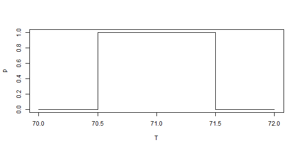
“Do the simple experiment”
Here is the fallacy in your first case. You can take it that the distribution of each range is uniform, range +-0.5. So the first reading looks like this:
The variance is 1/12. But when you take the sum of 71 and 72, the probabilities are convolved:
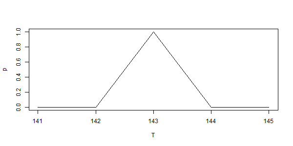
The range is +-1, but the variance is 1/12+1/12=1/6. When you sum all of them, the distribution is convolved again (with the running mean) and is
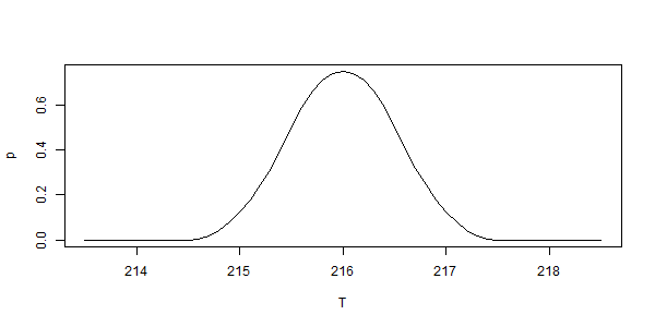
The range is now +-1.5, and the variance 1/4. To get the average, you divide the x-axis by 3. That brings the range back to +-0.5, but the variance is now 1/36. The range is theoretically 1, but with very small probabilities at the ends.
You can see that the distribution is already looking gaussian. This is the central limit theorem at work. The distribution gets narrower, and the “possible” range that you focus on becomes extreme outliers.
Kip – I think we have to keep pulling people back to considering the REALITY of what the ORIGINAL measurement purports to quantify.
Nick is correct. It is well established statistical theory that averaging of quantized signals can improve accuracy. The usual model is, however, based upon several assumptions. Rather than flat out rejection of the efficacy, which is well established, a counterargument should focus on the assumptions, and whether they are satisfied.
Quantization Noise Assumptions:
1) the data are homogeneous
2) the measurements are unbiased
3) the underlying signal is traversing quantization levels rapidly and independently
Under these assumptions, one can model quantization as independent, zero mean, additive noise uniformly distributed between -Q/2 to +Q/2, where Q is the quantization interval. The RMS of the error is then Q/sqrt(12). Averaging N samples then reduces the RMS to Q/sqrt(12N), and the averages are reasonably close to being normally distributed for large N. Such averaging is routine in a wide variety of practical applications, and the results in those applications do generally adhere to the model.
To what degree are these assumptions satisfied for the temperature series? Well, the data are not homogeneous, because temperature is an intensive variable. Its physical significance varies with the local heat capacity. And, the likelihood that the measurements are unbiased is vanishingly small, due to the sparse sampling, the ad hoc methods employed to merge them together, and the issue of homogeneity referenced above.
Assumption #3 is, in fact, the only assumption that likely does hold. Thus, I do not see the line of reasoning of this article as being particularly fruitful. It is attacking one of the stronger links in the chain, while the other links are barely holding together.
Thanks Nick. I like convolutions. Reminds me of a project is did on a scanning spectrometer once. Fine slits in the collimator give a sharp spectral resolution but sometimes light levels are too weak an you need to open up to wider slits. This convolutes the spectral peaks ( scanning wavelength ) with your first graph and causes broadening, losing resolution. In fact both inlet and outlet slits are finite leading to something like your second graph.
If the slits are not equal this leads to an isosceles trapezoid form convoluted with the scan signal. The fun bit is to try to deconvolute to recover the original resolution. 😉
The third one is quite a surprise. It’s obviously distorted but remarkably bell shaped. This implies that a three pole running mean would be a fairly well behaved filter, even with same window length each time, as opposed to the asymmetric triple RM I show here:
https://climategrog.wordpress.com/gauss_r3m_freq_resp/
Nick ==> Again, you are talking statistical theory — and trying to find probabilities, reducing inaccuracy of measurement through the simple process of — in the end — long division.
I don’t want to know the probability — I want to know the actual water level or the actual temperature — I want to know how close my measurement is to the real world true value -=- not theoretically how probably close my mean is to the actual measurement.
My instrument — the tide gauge — only guesses (mechanically) at the water level outside. Most of its guesses are within 2 cm of the actual instantaneous water level (outside the instrument) — some are not, but the kind folks at NOAA allow the system to throw out as many as necessary if they are more than 3-sigma different than the others in the same set (of 181 measurements), which allows me to meet the accuracy specification, which is, as discusses +/- 2 cm.
You may have as precise a MEAN as you wish, but you may not ignore the original measurement accuracy.
Kip,
“You may have as precise a MEAN as you wish, but you may not ignore the original measurement accuracy.”
You were wilfully misreading the advice from NOAA when you said:
“The question and answer verify that both the individual 1-second measurements and the 6-minute data value represents a range of water level 4 cm wide, 2 cm plus or minus of the value recorded.”</i
That wasn't what they said at all. They spelled it out:
“Sigma is the standard deviation, essential the statistical variance, between these (181 1-second) samples.”
That is statistical. It says that the probability of being in that range is 66%. You can’t get away from probability in that definition. And the probability reduces with averaging.
And you have tthe wrong measurement accuracy. The only thing here that could be called that is the 1mm resolution of the instrument. The +-20mm is a statistical association between the water inside and that outside. It is a correlation, and certainly is capable of being improved by better sampling.
i don’t think one can determine sea level to closer than 20mm, as at least with the Pacific, there is always more chop than that.
Nick Stokes ==> The sigma portion of the answer refers to the chart shown in the essay as:
which is a tiny segment of the official tide gauge report for the Battery for the 8th Sept 2017.
The rest of their answer is in specific answer to my specific question, exactly as quoted. I’ll forward you the whole email if it will help you understand. I have put NOAA’s portions in bold. This is an email thread, so the parts are in reverse time order, latest at the top.
For the time being, here is the text of the email string:
Kip,
Yes, it’s clear in that expanded string that their reference to sigma was to the variation of six-minute readings, not the 2cm estiamte. Sorry to have misunderstood that. But I still think the use of the 2cm (or 5mm) measures have to be considered as standard deviations. That is normal notation and practice. I see that the NOAA guy didn’t explicitly contradict you on that, but I don’t think he was confirming. Here is what NIST says about theexpression of measurement uncertainty:
“Standard Uncertainty
Each component of uncertainty, however evaluated, is represented by an estimated standard deviation, termed standard uncertainty with suggested symbol ui, and equal to the positive square root of the estimated variance”
Nick ==> It isn’t that I don’t understand that there is such as thing as “estimated standard deviations” or that they use them to make a standard statement about variation in measurements (of a static quantity measured many times).
If NOAA CO-OPS had meant “ui” or SD” or “1 sigma” or some other thing — then I would expect the specification sheet, and the support team there, so say so, and not repeatedly use the term “accuracy”.
I hope you realize that I am not arguing against the concept, when used in its proper place.
It simply can not be applied to a non-static, constantly changing, continuous variable measured at many different times with results reported knowingly as a range. The range used is the original measurement uncertainty and applies to all subsequent calculations.
Nick’s examples are exercises in the world of sampling statistics where his probabilities are fixed to some theoretical distribution (he’s using the normal distribution a lot) the parameters of which depend massively on the size of each sample. That should the first clue into how ‘magic’ the error reduction gets when he increases the size of the sample. Also enlightening is that these kinds of exercises assume you take the same-sized sample each time. The next step in his lecture series should now be on how one comes up with the parameters for a distribution of sample means when the sizes of the samples differ. At least that will make this more applicable to the tidal gauge / temp measure issue. But one still cannot overcome the limits of the observation. Kip doesn’t care about sampling error.
“he’s using the normal distribution a lot”
No, I’m not at all. The only theoretical number I used was the sd of the uniform distribution (sqrt(1/12)). It’s true that the central limit theorem works, but I’m not relying on it. It’s just using additivity of variance, and that will work equally for different sized samples, and for non-normal distributions.
Nick. When one invokes the central limit theorem one invokes the Normal distribution, because the latter is used to approximate the distribution of sample means. The standard deviation of that distribution gets smaller and smaller as you increase the size of each sample, and the shape of that distribution will look more and more Normal as you increase the number of samples. In a single sample, the standard error of the mean (SEM) is a sample estimate of the standard deviation described above. It is different from the sample standard deviation (SD). By itself, the SEM is a long-run estimate of the precision of the means of lots of samples. Both the SD and the SEM vary from sample to sample due to, at the very least, random sampling error. Under ideal circumstances, the sample mean is an unbiased estimator of the population mean. Under those circumstances, the sample mean will still not hit the population mean (because random sampling error), snd the SEM provides an expectarion of how closely the sample.meams should cluster together if you took a pile of additional samples each the same size as the first. Again. Precision. The mean of a sampling distribution of means will equal the population mean if both are distributed Normal. The central tendency theorem is invoked to assume that the distribution of sample means is Normal, even though the samples are drawn from a population that is non-Normal. This sets up valid null hypothesis tests that concern the means of sampling distributions of means and, say, a single sample.mean. It does not necessarily allow for unbiased estimation of the population mean using the mean of the sampling distribution of means, let alone our lonely single sample mean. So you are invoking the Normal distribution, a lot, when you refer tonthebcentral limit theorem. You’re dealing with sampling distributions.
“Nick. When one invokes the central limit theorem”
But I didn’t. I observed its effect. All my example did was to take means of various samples of daily maxima, and compare with the identically calculated means of data that had been rounded to integer values. No assumptions. The differences were small. I compared them to what is expected by additive variance (it matched) but that is not essential to the conclusion. I showed that the difference in means was nothing like the 0.29°C effect of rounding on individual data.
But in all this, I haven’t heard you support Kip’s view that measurement error passes through to the sample mean without reduction. You do say that it somehow adds differently, but don’t say how. How would you calculate the effect of observation uncertainty on the mean?
But this confuses the issue completely. The posting is not about removing the error from rounding, but from uncertainty in measurement. Your argument is utterly irrelevant to the question at hand.The post is addressing the physical fact that using a ruler that only measures accurately in millimetres twice won’t make it give you a measurement in picometers. You can’t use a high school ruler a million times to measure the size of an atom. Measurement accuracy does not improve with repeated samples.
o/t.personal comment.
you are not the _08 guy are you?
Probably not, just coincidence, but if you are you will know who I am (7).
@The Reverend Badger
If that’s directed at me I’m a frayed knot.
+1
Darkwing gets it. Nick is just obfuscating.
Nick,
You are missing Kip’s point. His assertion is that your January reading should be 26.0478 +/- 0.1.
+-0.05, I think. And he would assert that after rounding it should be +-0.5. But it clearly isn’t. I actually did it, for 12 different months. And nothing like that error is present in the means.
@Nick Stokes
You’re still missing the point. Why would the error be present in the means? There is no there there to begin with, in the means or otherwise. How can you say something is or isn’t present if it was never measured in the first place?
We are not discussing errors in means, we are discussing errors in measurement.
Pure hand waving, Nick.
Explain how century old temperatures, eyeball read from mounted shaded thermometers can be added to modern, never certified or recertified for accuracy, temperature thermistors?
Then an alleged average calculated out to four decimal places? Which by sheer absurdity only appears accurate.
e.g. Jan maxima average is 26°C, period.
Calculation of an alleged four decimal place version and/or difference does not represent greater accuracy than January’s 26°C.
It is all pretense, not reality.
Then you want everyone to accept that mishandling a Century of data accurately represent the entire and all potential weather cycles?
Hand waving, Nick.
“Hand waving”
No, it’s an introduction to a concrete example with real data.
Real data!?
You call four decimal place numbers from “0.n” maximum 1 decimal place physical measurements, “real data”?
That claim is a mathematical shell game using an imaginary pea.
Yes, you are hand waving.
“You call four decimal place numbers from…”
No, I call them calculated results. I need the decimals to show what the difference is. But the robustness of the calculation. To at least two decimals, you get the same result if you reduce data from 1 dp to 0dp.
You claim false value for your imaginary four decimal places.
Nor can you prove four decimal place value when using integers and single decimal place recorded numbers as data.
You use “robustness” just as the climate team does when they’re skating bad research or bad mathematics past people.
Nick Stokes ==> So let me get this right — you are saying that it does not matter at all what the original measurement accuracy is, because “Long Division will always reduce inaccuracies in measurement to negligible sizes if we just make a sufficient number of inaccurate, vague measurements.”
If we measured tide gauge water level only to the nearest foot (or meter), would you still like to insist that we can derive mean sea level to millimetric precision and accuracy? If so, why not go for an even tinier number — say 10,000ths of a meter? How low can you go with this? How about if we measured temperature to the nearest 10 degrees? Still get a perfectly defensible mean to hundreths of a degree?
Is your claim that measurement accuracy means nothing if you just have enough numbers to churn?
Get an eight foot pole that has markings at 1,2,3….8 feet.
..
Use this pole to measure 10,000 adult American males randomly selected. Each measurement is to the nearest foot.
…
When you sum all the measurements it will be roughly 58300 to 58400.
…
When you divide the sum by 10,000, you’ll get 5.83 to 5.84
…
Congratulations, you just measured the average height of an American male to less than the nearest inch. Pretty amazing considering your pole only has markings at one foot intervals!!!
Mark S Johnson,
Well if you have any stock in companies that manufacture highly accurate and highly precise measuring instruments you had better sell it. You have just let the cat out of the bag that anyone can get by with much cheaper, crude instrumentation if they just measure 10,000 samples.
Based on your remarks, I don’t believe that you have read my article that preceded the one Kip cited. Let me then share a quote from it:
“Furthermore, Smirnoff (1961) cautions, ‘… at a low order of precision no increase in accuracy will result from repeated measurements.’ He expands on this with the remark, ‘…the prerequisite condition for improving the accuracy is that measurements must be of such an order of precision that there will be some variations in recorded values.’” But, most importantly, you must be measuring the same thing!
Again Clyde, you post: “you must be measuring the same thing”
…
I posted: ” 10,000 adult American males”
…
See the difference?…….
Clyde Spencer: “Well if you have any stock in companies that manufacture highly accurate and highly precise measuring instruments you had better sell it. You have just let the cat out of the bag that anyone can get by with much cheaper, crude instrumentation if they just measure 10,000 samples.” When you are measuring the height of only one person, 10,000 samples are going to agree, and be up to 6 inches off with 95% chance of being up to 5.7 inches off when done with Mark S. Johnson’s 8-foot pole with perfect calibration and resolution of 1 foot. But if you are looking for an average height among 10,000 persons, Mark S. Johnson’s measuring pole can determine that with a much smaller +/- with 95% confidence. And if Mark S. Johnson’s pole has all of its markings being incorrect by the same amount or the same percentage, it can still be used to track growth or shrinkage of a large random population to the nearest inch if that changes by more than an inch, with high confidence.
It is a question of quantisation or resolution, ie precision, not accuracy. You should not use the two terms interchangeably. They have precise and different meanings.
It is not that the precision “means nothing” but less precision can be compensated by more readings.
Mark S Johnson writes
Except you’re an inch out on the true average and you couldn’t do it at all if the markings were at 3 foot intervals. You seem to want to ignore the measurements themselves when arguing how accurate you can be. Its a fatal mistake.
Mark S Johnson October 15, 2017 at 12:42 pm
“Congratulations, you just measured the average height of an American male to less than the nearest inch. Pretty amazing considering your pole only has markings at one foot intervals!!!”
What’s even more amazing is that you also got the height of Australian males to the nearest inch. I’m really impressed.
Too late. I helped developed such a system in 1995 at an electronics test and measurement company. The technique was developed many decades before that but only became economically viable in the 1990s due to the newer CMOS manufacturing capabilities.
Currently I have a Burr-Brown 24-bit ADC (59 ppb precision) with a 1 bit (+/- 50%) sampler in my stereo pre-amp. It sounds so good I run my analog record player through it. In 1995 we were happy to get 18 bits using the same technique for a digital multi-meter.
Your 1-foot interval for the American male population won’t work because the signal (actual heights) doesn’t vary by more than a foot. However, if you want 1/10th of an inch precision then measuring each male to 1-2 inches precision is quite sufficient. Just make sure when you calibrate your stick you calibrate your 1 inch tickmarks to 1/10th of an inch precision.
Peter
Peter Sable says: “Your 1-foot interval for the American male population won’t work because the signal (actual heights) doesn’t vary by more than a foot. ”
…
Nope, it will work because there are 6foot 3 inch males in the population, and there are 5 foot 2 inch males in the population. There are even some 4 foot 4 inch males and some 7 foot inch ones.
…
The key fact you don’t understand is that some males will be smaller than 5 foot 6 inches ,and some will be larger. It’s the relative proportion of each that determines the average.
I agree with Peter there. Calculating the average is trying to estimate ∫hP(h) dh where h is height, P is the pdf. The coarse ruler is like trying to evaluate the integral with quantiles. You can get a good approx with 1″ intervals, which is less than 1/10th of he range. But when you get intervals close to the range, the integration is likely inaccurate.
There aren’t enough in the population sample to span the range of 1 foot. you are right if you happen to know the exact mean of the population you could use a “are you taller or shorter” measurement and estimate the mean from that.
For an analog input signal to a 1-bit DAC it’s possible to know (or rather calibrate) the true mean of the population and then the proportion gives you sample average as you indicate I don’t think you know that mean a-priori with a population. Also, your population had better have an even distribution. I suspect there are more 6’6″ males in the population than 4’6″ males.
When the variance of the signal approaches the precision of the instrument, then the devil is in the details. We’re talking about 1degC precision with a 10degC diurnal variation, so not apples-apples to your yardstick example.
Nick & Peter….
…
Sorry to inform both of you, but, the numerical PROPORTION of 5 foot measures to 6 foot measures will contribute the most to determine the average when the sum of the measures is divided by 10,000. There will be some 4-foot measurements, and there will be some 7 foot measurements, but their numbers will be relatively small.
…
What makes any argument against my “8 foot pole” example fail, is that we know prior to executing my procedure, what the average is. Also known is how height is distributed. With these two facts, you will have a hard time showing my exampple failing.
Peter, the analogy of DAC is inappropriate. DAC sampling does not measure a population mean. It approximates an instantaneous value which is the antithesis of a population value.
OK, I tried it, and Mark’s method did still do well, with 1′ intervals. I assumed heights normally distributed, mean 5.83, sd 0.4. Centered, the expected numbers were
Weighted average is 5.818, so it is within nearest inch.
You are missing the point. What is the uncertainty of each of the daily maxima? Run your averages where the measurements are all at the top of range of uncertainty and then again when they are all at the bottom of the range. Now tell us what the “real” value is. If there are uncertainties, you just can’t assume the middle of the range is the correct reading.
Nick, we already went through this once and you haven’t learned how this works.
“As you’ll seen despite the loss of accuracy in rounding (To 0 dp), the averages of those 100 years, about 3000 days, does not have an error of order 1. In fact, the theoretical error is about 0.28/sqrt(3000)= 0.0054°C, and the sd of the differences shown is indeed 0.0062. 0.28 is the approx sd of the unit uniform distribution.”
You are making the same mistake as last time – you are leaving out the uncertainty of the readings, and treating them as if they are gold. You have calculated the centre of the range of uncertainty and called your construct the ‘theoretical error’. The uncertainty of each reading is 20mm up or down and you have shown nothing that reduces it.
You have provided an SD based on the data, but forgot to add the uncertainty for each reading, for which a different formula applies. You are trying to sell the idea that 3000 readings makes the result ‘more accurate’. The accuracy of the result is determined (only) by the instrument, which is why we rate the accuracy of instruments so we can pick one appropriate for the task at hand. You can’t just leave out the instrumental uncertainty because you have 3000 readings. They are 3000 uncertain readings and that uncertainty propagates.
It is a surprise to me that so many contributors do not understand this. Kip wrote it out in plan bold letters: measuring 1000 things once each with an inaccurate instrument does not provide a less-inaccurate result. That is the property of measurement systems – uncertainties propagate through all formulae including the one you show.
Measuring with a plus-minus 20mm tide gauge 1000 times over a 4000mm range does not provide an average that is known to better than plus-minus 20mm because that is the accuracy of the readings. Any claim for a more accurate result is false.
If you used the same equipment to measure the water level in a lake with waves on it, knowing that the level does not change, is a different matter in terms of how stats can be applied because that is taking multiple measures of the same thing with the same instrument. That still wouldn’t increase the accuracy, but the stats that can be applied are different. It certainly wouldn’t make the result more precise either because the precision remains 1mm. Your formula estimates quite precisely where the centre of the error range is located. Nothing more. The ‘real answer’ lies somewhere within that range, not necessarily in the middle as you imply. That is why it is called a “range”.
Crispin (wherever you are) ==> It nearly brings tears to my eyes to see that someone understands the issue so clearly.
Yours:
Crispin
“You have calculated the centre of the range of uncertainty and called your construct the ‘theoretical error’. The uncertainty of each reading is 20mm up or down and you have shown nothing that reduces it.
You have provided an SD based on the data, but forgot to add the uncertainty for each reading, for which a different formula applies.”
My example was of temperatures in Melbourne. But how do you “add the uncertainty”? What different arithmetic would be done? There seems to be a view that numbers are somehow endowed with original sin, which cannot be erased and has to be carried in the calculation. But how?.
In fact all my example did was to take a set of readings with high nominal precision, sacrifice that with rounding, and show that the average so calculated is different to a small and predictable extent. Any “original sin” derived from measurement uncertainty would surely be swamped by the rounding to 1C, or if not, I could round to 2C, still with little change. If the exact readings could have been optained, they would be a very similar series before rounding, and would change in the same way.
One test of these nonsense claims about irreducible error is to actually calculate a result (protagonists never do) and show the error bars. They will extend far beyond the range of the central values calculated. That does not make nonsense of the calculation. It makes nonsense of the error bars. If they claim to show a range over which the thing calculated could allegedly vary, and it never does, then they are wrong.
Nick, the errors at the different levels (observation vs. random sampling) will sum to give you the true estimate of error. If the errors are correlated (unlikely) then they sum but are also influenced by the direction and magnitude of the correlation between them. It is like Kip said, this isn’t typical undergrad stats, unfortunately (which is more a dig at oversimplified undergrad stats).
“Nick, the errors at the different levels (observation vs. random sampling) will sum to give you the true estimate of error. “
So how would you sum the observation errors? Say they amount to 0.5C per observation. Why would that sum differently than, say, 0.5C of rounding?
Kip wants to say that 0.5C observation error means 0.5C error in mean of 1000 observations. Do you believe that?
No, Nick, Kip Hansen is stating that the average does not mean anything without an error band of .5C., if the data going into the average had that error band.
Nick. Kip already mentioned it. The errors are essentially fixed, the observations finite and known. Therefore the SD will be +/- 0.5. (was it cm?) Var=(n/n)E{0.5^2}. SD = Var^0.5. This is your first level variance. Sum it with variance from each additional level of estimation. With all the different sites of measuring water level, each probably exposed to different factors which probably overlap sometimes from site to site, I would guess that sea level would be considered a random effect if this were a meta analysis. Variability (precision) within each site and variability in sea level betweem sites would need to be taken into account as well in order to get the ‘true’ unceetainty in the uber avergage.
RW,
“Var=(n/n)E{0.5^2}”
Do you mean 1/n? I can’t figure the second term, but it sounds a lot like you’re agreeing with Mark Johnson and me that the std error of the mean drops as sqrt(1/n). What you’re saying doesn’t sound at all like Kip’s
” the means must be denoted with the same +/- 0.5°F”
And what do you make of Kip’s insistence that ranges, not moments, are what we should be dealing with?
Nick. Yes 1/n like you are thinking but because the error is 0.5 for each observation the equation becomes n/n …0.5^2 ‘n’ times…i just pulled the n out of the summation (‘E’) per summation rules to make it easier for you to see thay it has no effect at that level. We are back to what Kip said originally. We have also established that the 0.5 +/- is a standard deviation as i think was said by someone already (you?).
The SEM is not SD/(n-1)^0.5 as someone else wrote, it is simply SD/n^0.5 . The n-1 only comes with the calculation of sample variance. Here, we use n for variance because we have the population of observations. We are not generalizing to a population of observations.
“because the error is 0.5 for each observation the equation becomes n/n …0.5^2 ‘n’ times…i just pulled the n out of the summation (‘E’) per summation rules to make it easier for you to see thay it has no effect at that level. “
You’ll need to spell that out in more detail. If you are summing n variances, the summands are, after scaling by the 1/n factor of the average, (0.5/n)^2. So the thing in front should be (n/n^2).
As for “We are back to what Kip said originally.”, no, Kip is very emphatic that 0.5 is not a sd, and we should not think of probability (what else?):
“In scientific literature, we might see this in the notation: 72 +/- 0.5 °F. This then is often misunderstood to be some sort of “confidence interval”, “error bar”, or standard deviation.”
Nick ==> Do you think there is anything you and I can agree on on this very narrow specific point? If so, pass it by me.
Kip,
I think no agreement is possible because you reject probability as a basis for quantifying uncertainty, and I insist there is nothing else. People here like quoting the JCGM guide; here is one thing it says:
3.3.4 The purpose of the Type A and Type B classification is to indicate the two different ways of evaluating uncertainty components and is for convenience of discussion only; the classification is not meant to indicate that there is any difference in the nature of the components resulting from the two types of evaluation. Both types of evaluation are based on probability distributions (C.2.3), and the uncertainty components resulting from either type are quantified by variances or standard deviations.
You like intervals. But
1) meaningful intervals rarely exist in science. Numbers lie within a range as a matter of probability; extremes of any order can’t be ruled out absolutely. If an interval is expressed, it is a confidence interval, perhaps implying that the probability of going beyond can be ignored. But not zero, and the bounds are arbitrary, depending on what you think can be ignored, which may differ for various purposes, and may be a matter of taste.
2) Intervals do not combine in the way you like to think. Science or Fiction set out some of the arithmetic, as did I and others. When you combine in an average, the only way the ends of an interval can stay populated is if all the measures are at that end. So it is one-sided, and takes an extraordinary coincidence.
You don’t have absolutes in science. Heissenberg insists that you might be on Mars. All the oxygen molecules in your room might by chance absent themselves. One does not think about these things because the probabilities are extremely low. But you can’t get away from probability.
The practical problem with your musings is that they describe a notion of uncertainty which is not that of a scientific audience, as the JCGM note shows. So it doesn’t communicate. I also believe that it just isn’t one that you could quantify or use systematically. That is what StatsFolk have learnt to do.
Nick ==> Well, I tried.
I wonder what’s wrong with me and all those engineers and other scientists that agree with me?
This shows nothing aside from how the number of significant digits you use has little influence on the standard deviation of a sample of sample means (i.e. the standard error of the mean). You are talking inferential sample statistics. All the gains you are referring to combat random sampling error. The post concerns uncertainty in the measurements themselves. These are different things. The former is hugely helped by taking more samples and/it increasing the n in each sample, whereas the latter is not overcome by this.
“You are talking inferential sample statistics. All the gains you are referring to combat random sampling error. The post concerns uncertainty in the measurements themselves. These are different things. “
They are. And the post is talking about the wrong one. In climate, many different kinds of measurement are combined. The post imagines that somehow the measurement uncertainty of each aligns, and can be added with no effect of cancellation. It doesn’t explain how.
There may indeed be some alignment; that would create a bias. An example is TOBS. People make great efforts to adjust for changes in that.
Nick writes
Another might be how the satellite chases the tidal bulge around the earth when doing sea level measurements such that month averages have biases.
Is temperature truly infinite in the continuum like time is, or does it have quanta associated with it like radiation?
I found a sample document to read, but I haven’t extensively studied quantum mechanics yet :
TEMPERATURE IN QUANTUM DYNAMICS
ALESSANDRO
SERGI
ABSTRACT
. What is the meaning of the thermodynamical temperature in quantum mechanics? What is its role in the classical limit? What can we say about the interplay between quantum and thermal fluctuations? Can we impose a constant-temperature constraint within dynamical simulations on quantum systems as we do in simulations of classical systems?
https://www.scribd.com/mobile/document/40884849/Temperature-in-quantum-mechanics
You are talking of at a theoretical level there you don’t measure at a theoretical level you measure with an instrument. The instrument has it’s own characteristics which often don’t precisely match the quantity being measured and it will shock many on this site because of their level of science that temperature is one of them.
So lets do this as basic as we can in quantum mechanics temperature is a “made up” statistic you can’t isolate it as a pure quantity. You actually need to combine several real quantities in QM to make what you measure as temperature. Temperature in classical sense was something that made a fluid inside a tube move up or down past some marks on the device. Later it got turning into roughly the movement speed of the molecules in classical physics. The problem comes with QM that you can have movement and momentum which can’t be isolated to our 3 dimensional world but can shown to be QM quantities.
So what the article is dealing with is you need to be very careful when trying to have temperature arguments in QM because you need to clearly isolate what you are calling temperature, it isn’t clear cut like in the classical sense. You see this in that QM can take temperatures below absolute zero, they aren’t breaking the laws of physics it’s just the thing you call temperature isn’t a pure thing and they are showing that by using QM techniques.
All of that is outside what is being discussed, you have a device which is measuring classical temperature. I am sort of having fun watching all sides try and follow thru the argument. No one has got it completely right and there is a big thing missing which is discussion of the measurement device itself.
I hope first explaining the QM basics and making the parties aware they need to think about the device. The article looks at the Sea Level device and it is on the right track. Nick, Rick and a few others are coming at it from statistics but they haven’t thought about the device itself. Kip is right in asking the question are you entitled to use the statistics and you need to work that out for yourself and what the underlying assumptions become.
“All of that is outside what is being discussed”
Kip (the author) calls temperature a continuum, using the word infinity or infinite. The article I linked to mentions kinetics as part of what temperature is at the atomic level which therefore indicates to me that temperature is indeed a continuum and not discrete (quanta / quantum).
I have a high interest in knowing the extreme details of temperature constructs because of my work involved in the Wattson Project, which isn’t scheduled for public introduction until January 2019.
The thing you are calling temperature is a continuum in classical physics. It is not anything in QM it is a made up thing to match what you measure in classical physics. I can’t be anymore blunt.
There is nothing to understand about temperature in QM it simply a construct of some quantities to match what classical physics describes. If you like it is like trying to measure a rainbow.
I should say if you are seriously going to try and understand it this is the bit you need to understand, but I suggest it will be meaningless without a QM background
https://en.wikipedia.org/wiki/Partition_function_(statistical_mechanics)
“[ Note: In a separate email, it was clarified that “Sigma is the standard deviation, essential the statistical variance, between these (181 1-second) samples.” ]”
My guess is this isn’t as odd as it sounds. But. “essential” was probably intended to be “essentially”?. And the standard deviation is the square root of the variance? My guess is that “variance” really should have been the less rigorous term “variation” Note that the statistical property “variance” has units of the variable under discussion squared and is often a disturbingly large number compared to the actual size of the errors.
Don ==> Yes, I should have added “(sic)” to the quote of the email — the correct word should have been “essentially”. The point of including this statement was for clarity. NOAA CO-OPS notes the sigma of the six minute readings as very small, but the “accuracy” as +/- 2 cm, for the same recorded “measurement”.
I don’t want to be pedantic, but this is a subject that I taught to laboratory technicians and engineers for many years.
Sorry MSJ, Kip is correct and you are wrong. A measurement uncertainty specification states the size of an interval around the indicated value within which the true value is thought to lie. Properly stated the MU specified should indicate the distribution type used to determine it – i.e. normal, rectangular or triangular and a confidence level – see the ISO Guide to the Expression of Uncertainty in Measurement (GUM). It is typically 2 times the standard uncertainty derived from calibration comparisons the a primary reference along with evaluation of additional sources of MU. There are always more than one.
When multiple measurements of something are made with a precise enough instrument they will invariably differ by some amount. The differences are considered random error and this can be reduced by averaging a number of measurements. But the random error is a source of uncertainty that is in addition to the instrument MU.
So, it I take 100 measurements with a +/- 2 cm instrument and get an average of 50 cm with a standard deviation of 1 cm the overall MU is +/- 2.32 cm at a 95% confidence level. [Note: there is math involved in this calculation: MU = (sqrt((2/sqrt(3))^2 + (1/sqrt(n))^2))*2].
In short, no matter how many measurements you make, the MU of the average is always greater than the MU of your instrument
Rick C PE, you do not understand the difference between measuring an individual item and sampling a population mean. There is no instrument capable of measuring the average monthly temperature of anything. The only way this can be done is by using a multitude of individual measurements arithmetically combined to yield an “average.” Hence the mathematics of statistical sampling must be invoked to determine the confidence interval of the SAMPLING.
…
You are at the mercy of the sqrt(N) where N= the number of observations used to determine the population mean.
Mark , what you have just done is to say because “there is no instrument capable of measuring the average monthly temperature of anything” we will ignore measurement error.
Imagine that you such a series of measurements and do the stats and state your uncertainty as +/-0.1 degree. You then check manufacturer’s spec for the thermometer and find that is was only calibrated to be +/- 1 degree of the true temperature.
this is part of measurement uncertainty which is not reflected by your statistics and never can be.
Mark
The sqrt(N) is a theoretical construct only valid when the individual sample uncertainty is negligible.
Ever heard of Nyqvist or signal to noise ratios? Statisticians often forget these ideas and even the field of metrology. Or how about the basic Scientific Method?
The idea is that you design the tools to fulfil the job. So if you require a certain maximum uncertainty you use tools that can give you that with multiple sampling.
Temperature measurements and even sea level heights were not recorded with instruments and processes designed to give real uncertainties of a tenth of expected values.
For example the typical variation of temperature anomalies is 0.1 K pre decade. So you need to design your system ideally with a systematic uncertainty of around 0.02 K or less, for decent signal to noise. 10 to 1 is better if that data is then processed and other results derived from it.
Mark: It is you who apparently does not understand that measurement uncertainty and sampling theory are two different things. The issue is the erroneous assumption that the error in instrumental measurement is random and symmetrically distributed about the ‘true’ value. This can never be known as there is always some possible bias. An instrument with a stated calibration uncertainty of +/- 2 cm could, for example, always be off by +1.5 cm and be considered acceptable (fit for purpose). Thus, no matter how many readings are averaged the answer will still have a +1.5 cm bias error. Here it should be noted that bias by definition is not known, or it would be corrected in the calibration process – e.g. “subtract 1.5 from the measured value”.
Sampling is actually a quite complicated issue. Key issues include assuring randomness of samples, number of samples relative to population size, consistent measurement instruments and technique, etc. From what I’ve seen in climate science, sampling is far from adequate to justify the precision typically claimed. Even in well controlled laboratory settings, assuring that samples are truly random and properly represent the population being studied is often difficult. In many cases either the value of samples that may be destroyed in the analysis process or the cost of making the measurements themselves make statistically proper sampling infeasible.
The application of normal statistics to estimate the range of a population mean from a sample mean (dividing the sample SD by the square root of n) is based on an inherent assumption that the measurement errors are random and normally distributed about the true value and that the sample is truly representative of the population from which the sample is drawn. I don’t think any of these conditions are met in the evaluation of annual mean temperatures or sea level.
One final thought. In the laboratory we often make measurements of samples to determine some specific property – e.g. measure the tensile strength of 30 samples taken from a coil of steel. Each measurement may have an uncertainty of 100 psi, but the SD of the sample results may be over 1000 psi. In such cases the MU is of little consequence. Thus, we always want to use instruments at are at least 4 to 10 times more precise than the inherent variability of what is being measured. If you want to measure mean air temperature to an accuracy of +/- 0.1 C, your thermometer should have an uncertainty of less than 0.025 C.
Rick C PE ==> Yours: “I don’t think any of these conditions are met in the evaluation of annual mean temperatures or sea level.”
Yes, that is exactly right. The StatsFolk insist on throwing
ourout the original measurement uncertainty (accuracy range of the measuring instrument) without first making sure that the requirements for applying their statistical analysis approach applies to the physical system and its measurements.They are entitled to find as “precise” a Mean as they wish — but they may not discard the original measurement uncertainty in doing so. If they insist that they can validly do so, then we could measure water levels to the nearest foot, or meter, or mile, throw out the known range of measurement uncertainty, and still derive a mean to millimetric precision.
Rick, perhaps you could write an article on this. You seem to be a lot more knowledgeable and qualified on the subject. This whole subject of uncertainty of measurement and claimed uncertainty is fundamental and has remained largely unchallenged for decades.
Sadly I doubt much will come out of the sporadic flow on comments here.
Rick C PE ==> Thank you for the support….few and far between.
The original measurement uncertainty is normally simply chucked out the window and the recorded figures treated as discreet measurements.
so refreshing to hear from someone who has a solid professional grasp of the topic — I have sympathy for those with stats training who “know the rule” but not the exceptions.
When I did the “mathematics and statistics” courses in about 1976 this stuff was treated rigorously. I do remember it was a hard course requiring lots of homework and clear thinking, and the teachers were really strict about getting it right. How very sad to think that the standards seem to have dropped somewhat.
As you say Kip,
Some people have done a reasonable level of maths and comprehend the difference.
Others don’t comprehend and probably never will.
Pointless to argue something that is beyond their ability, or willingness, to comprehend.
Rick. Perhaps you could answer this, then, which seems to be at the heart of the issue:
If I have some number years of Jan 1 noon temperature measurements, each accurate (as per the article) to +/- 0.5 deg, and I plot them on a chart and fit a line and observe a slope to that line, how many measurements should I take to be sure of a rising (or falling) trend? Or, how many +/- 20mm tidal measurements must I have to declare a 1mm/yr sea level rise?
Paul Blase ==> I’ll take a pass at your question while we wait upon Rick — I don’t mean to answer for him.
For your temperature example, two. It only takes two (2) data points to draw a line. That line is the “trend” of those two points. If the known measurement uncertainty is +/- 0.5°F, the difference between the first and second measurements would have to exceed that 0.5°F, to be certain that the measurements were, in fact, different at all. What you wouldn’t have is an understanding of anything as a result. You’d have just two dots, one different from the other.
To derive meaning from those two dots requires understanding the physical system, the underlying causes-and-effects, that produce “temperatures”, what the relationships between (in your example) annual same-day temperatures, what the variations or differences in these measured values mean and don’t mean, are my two temperatures different because of something in particular, or just different? Would it make sense to expect them to be the same? (This questioning goes on for some time). The same reasoning would apply if you had 100 years of Jan 1s, or a thousand years of Jan 1s.
Thank you. I suppose that we could flip the question around and say that IF a rise of (say) .1 deg per year or 1mm per year is important, how long until we can be sure that we actually have one?
You can’t catch up to find a trend outside the uncertainty. You may be able to see a trend by looking at the top, recorded, or lower range lines. However, the value of the temps in the trend will lie somewhere inside and you have no way to know an exact value. That is why using an average out to 1/100th or even 1/1000th is ridiculous. Throw a dart until it lands inside the range and you’ll be as accurate as any scientist!
First, I agree with Kip’s answer. But, while the question seems simple, the answer is quite complicated. In fact, I’m pretty sure there are many textbooks and scholarly papers on the question of trend analysis and in particular time series. The key issue is whether a trend calculated from a particular data set is an effect of some cause or a result of some inherent random variability – i.e. due to chance alone. Error in data measurement primarily adds to the potential for either missing a real trend or incorrectly concluding there is one. If we see a 0.3 C difference between years measured with an uncertainty of +/- 0.5 C each time, how do we know if it is a real difference or not?
But, even if we can conclude that an observed trend is likely real with a high confidence, this knowledge is of little value unless it has predictive value. Casino’s love folks who have a system that they think can predict the next roll of the dice or roulette number based on the trends they see in previous 10 or 20 trials. The stock markets have been trending up for some time, should you mortgage your house and invest based on this trend? Maybe buy stocks that have had the largest upward trend in the last 6 months?
Doing regression analysis (curve fitting) on time series data effectively makes the passage of time the “independent” variable. But the data being analyzed is typically not a function of time. Temperature and sea level are clearly influenced by many independent variables that change over time (and yes CO2 concentration is one of them). Many seem to cycle up and down at varying rates. Those who frequent this site can easily list many of them. The real question is does anyone have an adequate understanding of how all of these variables affect temperature and/or sea level to be able to accurately predict future climate? My own conclusion is that the earth’s climate system is an excellent example of a chaotic system and that prediction of future states is not possible.
By the way, we do know CO2 has increased quite steadily over the past 50+ years. However, if CO2 were indeed a primary control of temperature, there should be a strong correlation between them. But the data I’ve seen shows an R-squared of near zero. In my experience R-squared of less than 0.7 should be taken as a poor indicator of causation (more likely an indication of some unknown variable affecting both).
Kip: “So, it I take 100 measurements with a +/- 2 cm instrument and get an average of 50 cm with a standard deviation of 1 cm the overall MU is +/- 2.32 cm at a 95% confidence level.” What if an inaccuracy of determining a baseline measurement is not important and one is concerned about change from the baseline? Global average temperature is not as easy to determine as how much a determination of global average temperature changes. (The part of the world without official thermometers probably has a different average temperature than the part with official thermometers, but both parts of the world have high expectations of changing similarly in temperature when global average surface temperature changes.)
Or, suppose that the 2 cm instrument does not have an error of 2 cm or up to 2 cm, but merely rounds its output to the nearest 2 or 4 cm but is otherwise accurate, like Mark S. Johnson’s 8-foot measuring pole that measures the height of American adult males to the nearest foot? Or that you have a few hundred of these instruments with biases ranging from 2 cm upward to 2 cm downward in a random manner known to have a 99% chance of having average bias of no more than a few millimeters, or their biases are known to not vary from year to year. What do these mean for how little global sea level can change from one year or decade to the next and there is 95% confidence that sea level changed in the indicated direction +/- 99.9%? Or a change twice as great is known to be +/- 50% with 95% confidence?
Don K ==> And if the instrument merely rounds to the nearest foot?
Rick C PE
Thank you. Cogent and correct. You didn’t mention it but the ISO GUM “x 2” is there to create a confidence envelope around the measured value – a high confidence.
This bears repeating because this is how to propagate uncertainties through a calculation:
“In short, no matter how many measurements you make, the MU of the average is always greater than the MU of your instrument”.
Crispin
ISO TC-285
Kip — I think you/we are sort of skating on thin ice over a sea of statistical sampling theory here. Sampling theory is a serious, and very complex field that is very important to industry. It’s widely used to determine things like how many samples from a production run need to be tested to have a certain degree of confidence that the run meets predefined quality standards.
I know just enough about sampling theory to know that It’s really important and mostly beyond my abilities.
In your/our case, the issue is how to sample temperature/sea level so as to get a useful/meaningful estimate of values and changes in values.
Don K ==> Yes and no….it is not an inability to get a useful “estimate” — finding means is simple…and the rules and methods clear…..it is the meaning of the apparent precision of those means that is the question.
“We cannot regard each individual measurement as measuring the water level outside the stilling well”
Yes and no. Conceptually, the stilling well is just a mechanical low pass filter that removes high frequency noise caused by waves, wakes, etc. Hopefully, water level measurements made within the stilling well will yield the same value as would measurements made outside the well. With a LOT less measurement and computation.
Don K ==> The pragmatic, real world fact is that the measurement inside the stilling well is known and acknowledged to be different from that outside the well — at each 1-second instant that readings are made. NOAA is very careful in their illustration to make this point, and the CO-OPS support agent very careful to point out that each measurement is in reality ONLY expected to be within 2 cm (+ or -) of the water level outside the well.
You are exactly right that the stilling well is a mechanical “averager” or “filter” for the vast array of different waves and ripples and boat wakes and other disturbances of the water surface in a harbor (and having lived aboard boats and ships half of my adult life, I am far too familiar with the topic). But the supposition that this mechanical device does some sort of mathematical or statistical magic would be an error — it may be “like” some concept, but an engineer would explain that it simply does what it does, to the accuracy specified and tested in real use. That’s why I queried NOAA CO-OPS — and they confirmed this point.
Tide Gauges return instantaneous readings of the level INSIDE the stilling well to am accuracy of 1mm, and report a range of water level OUTSIDE the stilling well to +/- 2cm (usually — some of the 1-second readings are far off and must be discarded).
Kip,
You said, “Tide Gauges return instantaneous readings of the level INSIDE the stilling well to am [sic] ACCURACY of 1mm,…” I think that you mean a PRECISION of 1mm.
Clyde ==> I concede — NOAA refers to it as the “Resolution” of the inside-the-stilling-well measurement.
Kip is right. Simple thought experiment. Suppose you took any large number of daily readings of an actual daily temperature of 70.4999 degrees, every reading the same, due to the constant theoretical climate. Each would be reported as 70 degrees, and any number of days averaged would result in an average of 70, when the real average is actually almost half a degree distant.
In this very artificial example, the variability is so small that the roundings are totally correlated; the error far exceeds the variability. But with any real situation of temperatures or tide gauges, it is the opposite. If the error far exceeds the range of the data, measurement tells you nothing useful. But if you have a temperature range of say 10°, then rounding errors will no longer be correlated.
Yes, this is like measuring something with quantised digital sensor, eg and analogue to digital converter on some physical sensor. The results are quantised into steps. One technique in instrumentation design is to deliberately add a small amount of noise like +/- one quantum step BEFORE sampling. This means that you can average groups of ten sample and the quantisation of you results is the 1/10 of the previous step quantisation.
As long as the noise injected is normally distributed you have gained in resolution of the instrument at the cost of sampling ten times more often.
It should be noted that here you are measuring the SAME physical quantity at an interval where it is assumed not to have changed physically. You are not mixing ten different sensors !
Not the point, The argument is over measuring one thing once and then measuring a different thing another time and averaging the two gives you greater accuracy of “something” that the accuracy you had of the original things you measured.
I believe Phil (above ) is right: I base that on logic rather than stats. If today’s temperature is measured as 1 and yesterday’s as 2, then averaging them gives me 1.5. But that 1.5 is not a measurement of anything that actually happened, so the whole idea that it is “accurate” is nonsensical. I cannot measure something that does not and has not existed.
As Phil argues, smoothing a time series is not the same as averaging measurements of the same, unvarying thing.
I have to agree with Nick here. When you round to nearest integer you will adjust the measurements up or down +/- 0.4999 depending on what side of the zero point they were. Over multiple measurements each individual will fall “randomly” within the +/- 0.5 intervall.
MrZ
“Over multiple measurements each individual will fall “randomly” within the +/- 0.5 intervall.”
It might, or it might not. You have no idea, and that’s the point. You can’t just say it and then it is true.
Crispin ==> But “just say it and then it is true” is the basis of the strength of the StatsFolk argument. They have a standard method that has been drilled into them in Uni course after course, repeated until it dances before their eyes as a Universal Truth. But, like so so many things, the Devil is in the details — they know the rule but forget [or ignore] the exceptions and the required conditions for applying the rule.
I appreciate your enlightened input here.
Question: How much does the worlds river water run-off, and the soils it carries, rise the oceans level
over a year’s time.
Does the increase in soil deposits around the measurement site, effect the readings. The deposits have to increase the water level over time
“Question: How much does the worlds river water run-off, and the soils it carries, rise the oceans level over a year’s time”
Quick answer — not very much. More detailed answer. MOST of the water in run-off is derived from precipitation which, in turn, is ultimately fueled by evaporation … from the oceans.. Some is derived from storage in aquifers, but that is thought currently to be roughly offset by storage of water in new reservoirs.
“Does the increase in soil deposits around the measurement site, effect the readings.”
Conceptually, it doesn’t affect the readings because the measuring hardware is fixed to the old bottom.
In the grand scheme of things, sedimentation does represent a transfer of “dirt” from the land to the sea floor and thus raises sea level. But on a human timescale, the effect is surely negligible.
Additional note: Some older tide gauges using a mechanical float are said to have had a problem with sediment in the bottom of the settling well causing the float to bottom out at low tide. That causes the gauge not to record low water points properly.
Don K ==> Yes, that is an acknowledged problem. The PSMSL has a set of standard for records that it maintains — and I think that the old float gauges are excluded now. (I’d double check if it is important.)
Nice Cutting of a Gordian knot John. Isnt it fascinating how counter intuitive statistics can sometimes be giving rise to the rather intemperent divergences of opinion seen on this thread.
For the record I am with Kip, as physicist recalling ancient lab work
Alastair gray ==> Thank you sir. I am puzzled by the insistence of so many others on the use of statistical theory over practical real world example, use which ignores the rules for when those theories can be applied.
At least half the contributors on here would really benefit from being locked in the ancient lab. I can supervise Monday and Wednesdays for the rest of 2017. Any other volunteers? The project may well run into 2018 unfortunately.
Badger
It is clear who here works in a lab with real instruments and who does not. Thanks too, Alastair. Can you imagine claiming to report the bulk temperature of the oceans measured occasionally to 0.06 C and claiming it has risen by 0.001? The cheek!
When you start making claims on ‘world wide ‘ you really must face the reality of not just accuracy but ‘range ‘ Its is simply not enough to throw computing power , through models , at the issue. If you need a thousand or ten thousand measurement locations to deal with the scale, then to ‘know’ rather they ‘guess’ then that is what you should have .
And when it comes to weather or climate on a world wide scale we seem to be not even close to the coverage needed to make these measurement in a manner that supports the scientific value they are often attributed with.
One of the key statistical slight of hand tricks here is to pretend that thousands of measurement of SST are repeated measurements of the same thing, like it was some lab experiment.
In the context of AGW and attribution we are interested in assessing and attributing effects of changes in radiation flows on the surface temperature, ie for lack of better metrics we are using the ocean mixed layer as a calorimeter the measure heat energy. If we have sufficient data we can try the same thing on all water down to a certain depth and arguably get a more meaningful result.
So SST is not tens of thousand of measurements of some fixed quantity the “global temperature” since no such thing exists. There are many temperatures at different places for very good physical reasons. The “global mean temperature” is just that, it is a mean value : a statistic, it is not some physical quantity which we are taking thousands of independent measures of. In fact it is the sum which we are interested in, not the mean. The statistical confidence levels for the mean indicate how well the mean represents the sample and the confidence we can have that any given individual measurement will lie within the one or two std devs of the mean. This is not our confidence in the sum.
What we have is global array of little boxes of sea water for which we have a temperature, from which we want to estimate heat energy content. Now if we want the total energy content we will have several thousand individual measurements each with its own measurement error that we add together the get the global heat content.
There are many contributions to the uncertainty of such measurements some will average out others many be independent and thus considered orthogonal but will not average out others will be systematic and will not reduce at all.
Then we have to add changes over time of the measuring system, which itself is largely unknowable at this stage.
There is no simplistic answer like Kip’s +/-0.5 nor the usual +/- 2 s.d. which also ignores the nature of much of the uncertainty.
You are the first to get one big piece of the puzzle. Lets extrapolate the problem, for the tidal guages the wave background etc may be very different at different locations. Each guage at each location may have very different accuracy. In science it’s called the calibration problem.
What you want to ask the statistics group is what is the calibration and discrimination on their statistics.
Greg ==> My essay is about the original measurement uncertainty — of each and every individual measurement or its recorded value.
All the other stuff (and there is a lot of other stuff) is additive to the +/- 0.5° that derives from the original measurement uncertainty.
I have said nothing about standard deviations, which are not part of the story in my essay.
thanks Kip. You seem to be missing the point a bit.
There is a quantisation error in the recording method but there is also a lot of noise in the signal. With many measurements, averaging breaks down the quantisation. See my explanation of this effect and how it is dealt with in instrumentation design.
Leo makes a similar point later using an audio example.
Recording nearest degrees will cause a problem if the recording method changes and is not documented thoroughly and adjusted for. It is not a problem in itself if methods are consistent.
You are mistaken in asserting that the result can never be more accurate than a single reading.
Maybe you should try it. Take a dataset , do some averaging then truncate or round or whatever and show some figures. The very limited numbers you use in the essay do not examine the effect of averaging.
Greg ==> You are speaking only of mathematical results, and not real world measurement results, and your example works, of course, because that’s how long division works. It is a circular argument, in a sense.
Work out the little exercise in Author’s Comment Policy section — share your results below. You will find that the range of the mean is the same as the range of the original measurement. It can not be different.
Kip
I will go out on a limb here and say that the 20mm is based on observations in typical wavy tides. I am willing to bet a coffee that in windy places where the waves are higher, the 20mm claim is unsustainable. Just as one finds when taking measurements in the lab, the instrument can only perform well within a certain range of conditions. If they did some calibration exercise and arrived at the round number of 20mm, it is probably only reasonably true, and only in ‘standard conditions’. The reason is that as discussed above, the stilling well level is known to deviate from the water outside, and it cannot possibly have a perfectly linear error up and down over a range of sea conditions. On a calm, it might be 8mm and in stormy weather, 50mm. I am sure they use 20mm as a “general case” and live with the consequences. The fact that there are ‘outliers’ indicates there are generalisations and assumptions behind that 20mm figure.
Crispin ==> Tide Gauge specs are created by technical bureaucrats and committees, International bodies of sea level and tide people — I bet I could find, given a few hours and the patience to spend them, the very technical paper that describes the hows and whys of the spec at ±2cm. I may give it a go later this week.
Re the “stilling” chamber. As Don K says there is a “low pass filter” which hopefully eliminates the effect of high frequency noise from waves and wakes. Note that depending on the location, and the design, it is unlikely to eliminate the low frequency noise from swell – easily 9 second period and in a bad location more. Further, because of the friction in the filter, the level inside will be different from that outside – when the tide is rising the interior level will be lower, and when the tide is falling the level will be higher.
As a real – ie geographical – low pass filter, I refer you to the Rip at Port Phillip Heads. Here a narrow channel connects the open ocean and Port Phillip. Consider starting from an instant when the levels inside and outside are the same. Then as the tide outside rises, water pours in through the Rip, and the tide rises inside Port Phillip. When high tide is reached outside, the water is still pouring in, and continues to do so until the outer water level has fallen to the level inside. At this time, high tide is reached inside Port Phillip, while the outside water level is approaching half tide.As tide level outside continues to fall, water commences to pour out, and the tide level inside Port Phillip starts falling. Given the range of tide outside, and the tidal range inside, the six hourly period (approximately) between high and low tide outside is offset by nearly three hours (approximately) inside.
This is on a far greater scale than that in the tide gauge, nevertheless, a similar situation. Hopefully the difference between inside and outside is rather lower!
Re the accuracy of readings. As a cadet on a cadet ship in the 1950s we had to take sea water temperatures using the bucket method. We had to read – estimate – the temperature to the nearest 0.1 degree. I cannot recall if it were in Fahrenheit or Celsius – as the thermometers were supplied by the UK Met Office I suspect that Celsius was used – I remember that in the coded message we had to insert a C or F for the readings of all temperatures. Note exactly on a degree line is easy to observe, and exactly half way between is also easy. A third or a quarter is also easy to estimate, and this gives 0.3 or 0.7, and it is fairly easy to see if it is a little more than a quarter – hence also 0.3 or 0.7, or a little less, hence 0.2 or 0.8, and if it is a tad more or less than the actual mark, then it is either 0.1 or 0.9. In good weather, the reading would be good. With a strong breeze blowing, and rain or sleet, it would be difficult to get better than to the nearest 1 degree. And in a howling gale, often it would not be possible to get the bucket in the water – it would be blown sideways so much it never reached the water.
Presume the Met Office found our reports valuable – there weren’t too many ships which reported and did so regularly every 6 hours, at 0000, 0600, 1200 and 1800 GMT.
I have zero experience with mechanical low pass filtering, but I’d expect them to have a breakover frequency with a smooth attenuation of frequencies above that point — probably 6db per octave. So, I’d expect swells to be attenuated, but not as much as higher frequency phenomena. That’s a guess.
dudleyhorscroft ==> Thanks for sharing your personal experience with water temperatures made from ships with the bucket method.
Stilling wells work much like tides through a narrow channel — the water level inside the harbor is nearly always different than outside. They have a hole in the bottom that allows water in and out as the water level outside changes, causing the water inside the well to rise and fall as well — but not in sync and not equal in magnitude — the physical system averages the rising and falling at different “frequencies” and magnitudes in such a way that NOAA CO-OPS is fairly certain that, by design, the very accurate and precise measurement inside the stilling well will be within 2 cm (+/-) of the actual water level outside the stilling well at that instant. It doesn’t always work, and some 1-second values have to be discarded as way out of range (3 sigma rule).
Kip — FWIW, Here are some links I bookmarked over the past couple of years about how tidal gauges work and their problems
(Performance of modern tide gauges: towards mm-level accuracy …) http://www.vliz.be/imisdocs/publications/258249.pdf
(General discussion of tidal gauges) https://web.archive.org/web/20160810171211/http://noc.ac.uk/science-technology/climate-sea-level/sea-level/tides/tide-gauges/tide-gauge-instrumentation
(Discussion of sea level measurements in the Falkland Islands–of interest because James Ross made detailed observations of sea level there in 1842 using benchmarks that are still accessible) http://onlinelibrary.wiley.com/doi/10.1029/2010JC006113/full
(The Difficultiesin Using Tide Gauges to Monitor Long-Term SeaLevel Change) https://www.fig.net/resources/monthly_articles/2010/july_2010/july_2010_hannah.pdf
Don K ==> Thank you, sir. Very helpful.
Cook-ery with numbers
97% (+/- 98.8%) with very high confidence (because ‘Climate Science™’ is all about confidence not verification or proofs).
Your position does not seem to agree with the international guideline: Evaluation of measurement data — Guide to the expression of uncertainty in measurement
See section:
“4.4.5 For the case illustrated in Figure 2 a), it is assumed that little information is available about the input quantity t and that all one can do is suppose that t is described by a symmetric, rectangular a priori probability distribution …”
and
“4.2.3 The best estimate of σ 2(q) = σ 2 n, the variance of the mean, is given by …”
It seems as if the origin of the disagreement is related to:
“G.2.1 If Y=cX +c X +…+c X =ΣN cX and all the X are characterized by normaldistributions,…
then the resulting convolved distribution of Y will also be normal. However, even if the distributions of the Xi are not normal, the distribution of Y may often be approximated by a normal distribution because of the Central Limit Theorem. …”
It would be interesting if you, with reference to this guideline, could identify exactly the source of the disagreement. After all, if there is an error in this standard, you need to identify that error quite precisesly:
“The following seven organizations supported the development of the Guide to expression of uncertainty, which is published in their name:
BIPM: Bureau International des Poids et Measures
IEC: International Electrotechnical Commission
IFCC: International Federation of Clinical Chemistry
ISO: International Organization for Standardization
IUPAC: International Union of Pure and Applied Chemistry
IUPAP: International Union of Pure and Applied Physics
OlML: International Organization of Legal Metrology ..”
Science or Fiction ==> Did you personally undertake the simple exercise described in the Author’s Comment section?
I did more than that:
I generated 100 set of 2000 random temperatures between 0,00 and 10,00 (Unit doesn´t matter)
(Let us call these sets ´real temperatures´.)
I calculated the average of each set.
For each temperature I then:
Rounded the temperature to the nearest integer.
(Let us call the resulting sets ´rounded temperatures´)
Calculated the average of each set of rounded temperatures.
I then:
Calculated the standard uncertainty of the average value of the rounded data set in accordance with the Guide to the expression of uncertainty: Result: 0,006
Which means that for the hundred sets I would expect to see a maximum difference between the averages in order of magnitude 3 – 4 standard uncertainties = 0,018 to 0,024
For the 100 sets, I then calculated the difference between the average of the ´real temperatures´ and the ´rounded temperatures.
I then found the maximum difference between the two average values for the 100 sets:
Result: 0,021.
I repeated the test two times more –
Results: 0,023 and 0,021
The result was exactly as I expected on the basis of the ´Guide to the expression of uncertainty in measurement´.
More than that, in terms of your terminology:
The accuracy of the mean, represented in notation as +/- 0.5, is not identical to the original measurement accuracy. [of each reading]
Hence, the results of this test did not support your position.
S or F ==> Try the experiment as I defined it …. see if the range of possible means is the same as range of the original measurement uncertainty. It is, very time.
Youare working a different problem, about probability and the precision of means.
“Try the experiment as I defined it …. see if the range of possible means is the same as range of the original measurement uncertainty. It is, very time.”
You are right! The range of possible errors of the mean is the same as the range of possible errors for the individual measurements. 🙂
However, that is also an useless conclusion.
I will explain why.
Let us say the resolution is 0,1 DegC.
For the average to be 0,5 DegC too high, all measurements have to be 0,5 DegC too high
The probability that one measurement is 0,5 DegC too high is 1/10
The probability that two measurements is both 0,5 DegC too high is 1/10*1/10=1/100
The probability that n measurements are all 0,5 DegC too high is 1/(1*10^n)
The probability that 80 measurements are all 0,5 DegC too high is 1/(1*10^80)
Given that 1*10^80 has also been proposed as estimate for the number particles in the Universe, I think the conclusion is pretty clear. The probability that the error of the mean is equal to the error of each measurement is vanishingly small – as in completely unlikely, for a relevant number of measurements.
Hence, your point that:
“The accuracy of the mean, represented in notation as +/- 0.5, is identical to the original measurement accuracy — they both represent a range of possible values.”
is right, but absolutely useless.
S or F ==> Thank you acknowledging that the central point of the essay is correct — even if you don’t agree with the rest. That’s a sign of intellectual honesty, and I recognize and appreciate it.
“Usefullness” is a complex and complicated topic and may be beyond the bounds of this particular essay, except that the acknowledgement that the true accuracy of the “overly precise” means in many fields of research are omitted from the results — nearly always in press releases, often in published conclusions, and very often in future application.
One way to look at the temperature data is to first imagine that we use the current system of using integers to represent the 1°-range. We then look at a million measurements in the range, and you say that the chance, the probability, of all measurements being “0.5 too high” is infinitesimal. However, the same is exactly as true for all measurements being very near the integer.
Say we then change our approach and set the recorded values as “integer.5” to represent the range from “integer-1” to “integer+1” — the same 1° range, but centered on the .5. Now it would appear that values near the integers would be outliers, and the values near the .5 are “more probable”.
The probability estimation is not true by either scheme — in other words, not true in the real world.
Just a thought.
«We then look at a million measurements in the range, and you say that the chance, the probability, of all measurements being “0.5 too high” is infinitesimal.”
To be precise, 80 measurements is more than enouh to make that conclusion
“However, the same is exactly as true for all measurements being very near the integer.»
I´m not so sure about that. If we define the error of the average of the measured temperatures as: the difference between the average of the real temperatures and the average of the measured temperatures:
The probability for the error being in the 0,1 DegC interval around the true average is actually the higher than the probability for the error being in any other 0,1 DegC intervals.
To understand that, I think we first have to take a look at the following statements in your article:
«Any difference of the actual temperature, above or below the reported integer is not an error.»
I would say that if a high precision thermometer displays 0,5 DegC, and the measurement result is reported as 1 DegC, an error of 0,5 DegC is committed in the measurement process.
That interpretation is also in accordance with the definitions in Guide to the expression of uncertainty (GUM): «B.2.19 error (of measurement): result of a measurement minus a true value of the measurand»
The next statement we need to have a closer look at is:
«These deviations are not “random errors” … »
If the real temperature is a random and continuous variable that can take on any value within a range that is larger than the magnitude of the rounding (see definition of in GUM C.2.2).
Then
The error, by rounding, that is made in each measurement, is indeed random within a 1 DegC range
The second part of that sentence is correct:
«These deviations …. are not “normally distributed”.»
But we can specify the distribution. Actually, the probability distribution for the error is termed a rectangular distribution (GUM 4.3.7 and 4.4.5 ). I can not even think of a more perfect example of a rectangular distribution.
And now comes the crux.
A combination of a little handful of measurements having equal rectangular distribution will approximately have a normal distribution (GUM G.2.2 ):
«EXAMPLE The rectangular distribution (see 4.3.7 and 4.4.5) is an extreme example of a non-normal distribution, but the convolution of even as few as three such distributions of equal width is approximately normal.»
This, I am not good to explain, but it has been demonstrated. See (GUM G.2 Central Limit Theorem) or Wikipedia on ´Central Limit Theorem´ . (I don´t think William Connolley has messed up that article yet. 🙂 🙂
As
the central limit theorem postulates that the combination of a handful or more of rectangular distributions of equal width will approach a normal distribution,
and
a normal distribution has highest probability density at a range around the central value
then
the probability for the error of the average being in the 0,1 DegC interval around the true average is actually the higher than the probability for the error being in any other 0,1 DegC intervals.
I believe that another way to think of it is that the range near the real average is the range that has the largest number of possible combinations of individual measurements. I believe that follows from the central limit theorem.
Central limit theorem with square or ‘rectangular’ distribution is ‘easy’ to explain. The key is in taking the average. The average will always ‘pull’ towards that middle value (along the x axis in that distribution graph). It’s more likely to fall into the middle values than the extreme ones. Think if it this way, each observation could yield a value from the left it right of the middle x value. Averaging them together just brings you to the middle. Think of a coin toss. 2 flips. Heads 0 Tails 1. 2 of those outcomes yields .5, 1 yields 0, and the remaining one yields 1. Voila, kinda normal-looking already. Do 100 flips and so on and eventually you’re into Normal curve land.
But this is just sampling statistics in a fun world where the theoretical distribution is known and you pluck observations from it pretending like you didn’t just fundamentally constraints the entire process to give you a fixed result as the central limit theorem indicates.
The magic of the central limit theorem…
…Is also a sort of unrealistic aspect of the central limit theorem. The averages of many variables are Normal distributed when you take an ‘approaching infinity’ number of samples, but the averages of other variables are not distributed Normal when you do the same procedure. In the real world, we often do not know the distribution of the variable we measure, and the number of samples we take is limited, so we cannot really test whether or not the central limit theorem holds. Invoking the central limit theorem to conjure a Normal distribution is invoking an assumption that is probably not even remotely testable. So it is a big qualifier in many cases – and statisticians are explicit when they invoke it.
But this all doesn’t do anything for getting rid of the uncertainty in the observation. That kind of random error and random sampling error are different sources of error.
While the accuracy diacussion is interesting, it is not important to the issue of WARMING, which is the determination of rate of change. The confidence in the slope of the temperature line is certainly related to the precision, not the accuracy, and it is here where sampling makes a difference.
You are sort of dancing with the second problem the stats group haven’t addressed. So hold your thought about the rate of change, and lets divid the space in two one half increasing at rate X and one at rate Y.
So what does your average rate represent?
Okay now divid the space into 4 X & Y remain the same but U is not changing and W is going down at a slow rate. Now what does your average rate represent?
You can be certain about the average rate but what does that really mean to any one of the 4 sections of sample space you need to do something very important as the next step in science. I am interested to see if you know what that is.
BRILLIANT ! Thanks LdB, you are making me work hard to retrieve stuff in my brain from over 40y ago,
I love this blog – good job I am half (+/- 0.125) retired!
Roger ==> As to the “slope of the trend line”…..the original measurement accuracy comes into play when the uncertainty range is applied to the resultant means. If the means are all within the uncertainty of the original measurement, then assigning a difference to the various means is a dicey proposition. If the accuracy of temperature measurements are in the +/- 0.5°F range, and all the means fall within this range, then there is uncertainty that the means are actually different.
Enthalpy is a measurement of energy in a thermodynamic system. It is the thermodynamic quantity equivalent to the total heat content of a system. It is equal to the internal energy of the system plus the product of pressure and volume.
https://en.wikipedia.org/wiki/Enthalpy
It is the change in total energy of the earth (system) that is important. Not including atmospheric pressure and water content (humidity) in calculations is another source of error.
rovingbroker,
Which raises another question. Because temperature is serving as a proxy for energy, how certain are we that there haven’t been long-term changes in humidity?