Guest Essay by Kip Hansen
There has been a lot of news recently about exoplanets. An extrasolar planet is a planet outside our solar system. The Wiki article has a list of exoplanets. I only mention exoplanets because there is a set of criteria for specifications of what could turn out to be an “Earth-like planet”, of interest to space scientists, I suppose, as they might harbor “life-as-we-know-it” and/or be a potential colonization target.
One of those specifications for an Earth-like planet is an appropriate average surface temperature, usually said to be 15 °C. In fact, our planet, Sol 3 or simply Earth, is very close to qualifying as Earth-like as far as surface temperature goes. Here’s that featured image full-sized:

This chart from the Chemical Society, [shows] that Earth’s observed average temperature should be about 15°C, and note that our atmosphere contains mostly Nitrogen (78%), Oxygen (21%) and Argon (0.9%) which makes up 99.9% of the total — leaving about one-tenth of one percent for the trace gases water (H2O and CO2).
Let’s look at the thermometer:

We see the temperatures believed to exist on the surfaces of the eight planets and Pluto (poor Pluto…).
The ideal Earth is right there sat 15°C or 59 °F.
Mercury and Venus are up at the top, one due to proximity to the Sun and the other due to a crushingly dense atmosphere, well out of range for Earth-like planets.
Mars is down below the freezing temperature of water, due to distance from the sun and mostly a lack of atmosphere coming in at 70°F (20°C) near the equator but at night plummeting to about minus 100° F (minus 73°C) with an estimated average of about -28°C. The average is a little low, but mankind lives on Earth in places with a similar temperature range, at least on an annual basis, so with adequate shelter and clothing (modified for lack of breathable atmosphere), it might do.
The other four planets and Pluto (poor Pluto) don’t have a chance of being Earth-like.
This next thermometer shows that Earth provides a temperature range suitable for human and Earth-type life, ranging from 56.7°C (134°F) at the high end down to -89.2°C (-128.6°F), with an average of 15°C (59°F).

Like Mars, Earth has a comfortable average that falls easily in what most people would consider to be a comfortable range, avoiding extremes, if properly dressed for the weather. For me, a southern California surfer boy by birth, 59°F (15°C) is sweater weather – or more properly, Pendleton wool shirt weather. 59°F (15°C) is the average Fall/Winter temperature of the surf at Malibu and most of us required wetsuits that would keep us warm in the water.
 Taking a closer peep at the middle of our little graphic, we see that the IDEAL Earth-like planet would have an average surface temperature of 15°C. But, in the 1880s through 1910, we were running a bit cool — 13.7°C. Luckily, after the mid-century point of 1950, we started to warm up a little and got all the way up to 14°C, just 1°C short of the ideal.
So, how have we done since then?
There is good news. Since the middle of the last century, when Earth was running a little cool compared to the ideal Earth-like temperature expected of it, we have made some gains.

By 2014, Earth has warmed up to an almost-there 14.55°C (with an uncertainty of +/- 0.5°C).
With the uncertainty in mind, we can see how close we came to the target of 15°C. The uncertainty bracket on the left for 2014 almost reaches 15°C.
2016 was a banner year, at 14.85°C and could have been, uncertainty taken in, a tiny bit over 15°C!
The numbers used in this image come from NASA GISS’s Director (and co-founder of the private climate blog that he and his pals work on while being paid by the government with your taxes) Gavin Schmidt. They are from his blog post in August 2017 — and, as always, have already been adjusted to be a bit higher. The current, adjusted-higher, numbers show 2017 0.1°C lower than 2016, which is what I have used.
That RealClimate blog post is quite a wonderful thing — it reveals to us several things, some of which I have written about in the past, which is the part I quote under the image. Dr. Schmidt kindly informs us about one of the miracles of modern climate science. This miracle involves taking data that has rather wide uncertainty — a full degree Centigrade wide, being plus 0.5°C or minus 0.5°C and turning it to accurate and precise data with almost no uncertainty at all!
Dr. Schmidt explained to us why GISS uses “anomalies” instead of “absolute global mean temperature” (in degrees) in the blog post (repeating the link):
“But think about what happens when we try and estimate the absolute global mean temperature for, say, 2016. The climatology for 1981-2010 is 287.4±0.5K, and the anomaly for 2016 is (from GISTEMP w.r.t. that baseline) 0.56±0.05ºC. So our estimate for the absolute value is (using the first rule shown above) is 287.96±0.502K, and then using the second, that reduces to 288.0±0.5K. The same approach for 2015 gives 287.8±0.5K, and for 2014 it is 287.7±0.5K. All of which appear to be the same within the uncertainty. Thus we lose the ability to judge which year was the warmest if we only look at the absolute numbers.”
So, by changing the annual temperatures to “anomalies” they get rid of that nasty uncertainty and produce near certainty!
 Source: https://data.giss.nasa.gov/gistemp/graphs_v3/ annotated-kh
Dr. Schmidt and the ClimateTeam have managed to take very uncertain data, so uncertain that the last four years of Global Average Surface Temperature data, when straightforwardly presented as degrees Centigrade with its proper +/- 0.5°C uncertainty, cannot be distinguished from one another, have now, through the miracle of “anomalization” been turned into a new, improved sort of data, an anomaly, which is so precise that they don’t even bother to mention the uncertainty — except to add (at least on the above graph) a single uncertainty bar for the modern data which is 0.1°C wide, or in the language used in science, +/- 0.05°C. The uncertainty in the Global Average Surface Temperature has magically become a whole order of magnitude less uncertain…. And all that without a single new measurement being made.
The miracle is accomplished by the marvel of subtraction! That is, one simply has to take the current temperature in degrees, which has an uncertainty of +/- 0.5°C, and subtract from that the climatic-term mean (current 1981-2010) and “voila” — the anomaly with a wee tiny uncertainty of only +/- 0.1°C.
Let’s see if that really works:

Here’s the grid of all the possibilities with a range of +/- 0.5°C for the 2015 temperature average in absolute degrees, and the 1981-2010 climatic mean in degrees, with the same +/- 0.5°C uncertainty range, both of which are given by Dr. Schmidt in his blog post. One still gets the +/- 0.5°C or 1°C wide uncertainty range. It did not magically reduce to a range one-tenth of that — it didn’t turn out to be 0.1°C wide as shown in Dr. Schmidt’s graph. I’m pretty sure of my arithmetic, so what happened?
How does GISS justify the new-improved wee-tiny uncertainty? Ah — they use statistics! They ignore the actual uncertainty in the data itself, and shift to using the “the 95% uncertainties on the estimate of the mean.” Truthfully, they fudge on that a little bit as well, which you can see in their original data. [ In their monthly figures, the statistical uncertainty (+/- 2 Standard Deviations) is a bit wider than the illustrated “0.1°C”.]
So rather than use the actual original measurement uncertainty, they use subtraction to find the difference from the climatic mean and then pretend that this allows the uncertainty to be reduced to the statistical construct of the “uncertainties” of the mean — standard deviations.
This is a fine example of what Charles Manski is talking about in his new paper:
“The Lure of Incredible Certitude”, a paper recently highlighted at Judith Curry’s Climate Etc. While Dr. Curry accepts Manski’s compliments paid to climate science based on his perception that many “Published articles on climate science often make considerable effort to quantify uncertainty.”, we see here the purposeful obfuscation of the real uncertainty of Global Average Surface Temperature annual data, replacing the admitted wide uncertainty ranges with the narrow “uncertainties on the estimate of the mean”.
Graphically, it looks like this:

Although I was a semi-professional magician in my youth, I have nothing that compares to the magic trick shown above — a totally scientifically spurious transformation of Uncertain Data into Certain Anomalies, reducing the uncertainty of annual Global Average Surface Temperatures by a whole order of magnitude — using only subtraction and a statistical definition. Note that the data and its original uncertainty are not affected by this magical transformation at all — like all stage magic, it’s just a trick.
A trick to fulfill the need of the science field we call Climate Science to hide the uncertainty in global temperatures — an act of “disregard of uncertainty when reporting research findings” that will “harm formation of public policy.” (quotes from Manski).
The true answer to “Why does Climate Science report temperature anomalies instead of just showing us the temperature graphs in absolute degrees?” is exactly as Gavin Schmidt has stated — if Climate Science used absolute numbers they annual temperatures would “All of which appear to be the same within the uncertainty. Thus we lose the ability to judge which year was the warmest if we only look at the absolute numbers.”
Thus, they use anomalies and pretend that the uncertainty has been reduced.
It is nothing other than a pretense. It is a trick to cover-up known large uncertainty.
# # # # #
While I was preparing this essay, I thought to attempt to illustrate the true magnitude of the recent warming (since 1880) in a way that would satisfy the requirements of a Climatically Important Difference. Below we see the UAH Lower Troposphere temperatures (even these as errorless anomalies) graphed at a scale of temperatures allowed in my personal living quarters before our family resorts to either heating or cooling for comfort — about 8°C (15 °F — as in 79°F down to 64°F). Overlaid in light blue is a 2°C range, into which the entire most recent satellite record fits comfortably and in purple, the prescribed 3-to-3.5°C comfort range from the Canadian Centre for Occupational Health & Safety for an office setting. If the office temperature varies more than this, then the HVAC system is meant to correct it by heating or cooling. As we can see, the Global Average lower troposphere is very well regulated by this standard.
 An interesting aside is that the Canadian COHS allows an extra 0.5°C in the winter, increasing the comfort range to 3.5°C, accounting for the differences in perception of temperature during the colder months.
# # # # #
Author’s Comment Policy:
Hope you enjoyed this rather light reading.
I am not so convinced by the hopeful thinking of astronomers regarding exoplanets. I believe they are out there (the planets, not the astronomers), and for the record I believe there are other intelligent beings out there as well, I just have serious doubts that our rather primitive instruments can identify them at such great distances.
For you budding scientists out there, Gavin Schmidt has given you a useful tool for turning your sloppy uncertain data in highly certain data using nothing more complicated than subtraction and a dictionary. Good luck to you!
Feel free to leave your interpretations of what the GISS Temp global graph in absolute temperatures (degrees) really tells us based on the two uncertainty ranges shown.
Oh, and against all odds, some things are better than we thought. The Earth, if we allow her to warm up just a tiny bit more, will finally be at the expected, ideal temperature for an Earth-like planet. Who could ask for more?
# # # # #
Good comments Kip. The people who want to get rid of that nasty uncertainty probably think denial is a river in Egypt. Another characteristic for an earth-like exoplanet would be a magnetosphere, wherein the gases that form an atmosphere are protected from solar winds.
our atmosphere contains mostly Nitrogen (78%), Oxygen (21%) and Argon (0.9%) which makes up 99.9% of the total — leaving about one-tenth of one percent for the trace gases water (H2O and CO2).
I think this is wrong. Water vapour makes (ON AVERAGE) 1% of our atmosphere (this was the case last time I checked). The other percentages add up to 99,9% because those values are their concentrations IN ABSENCE OF water vapour. They are generally very well mixed, which is totally not the case for water vapour, that’s why the water vapour concentration is provided separately.
Exoplanets… fantastic
And on current technology at least 40,000 years away.
This is a very interesting article and demonstrates the miss use of statistics. But the problems are even deeper rooted since it is absurd to claim that there is GLOBAL data going back to the 19th century. Even in the mid 1950s, the Southern Hemisphere data, at any rate that south of the tropics, is largely made up as Phil Jones so candidly noted in the Climategate emails. In truth, we only have worthwhile data covering teh Northern Hemisphere.
Then the data has been so heavily massaged with adjustments exceeding 1 degC to render it worthless for scientific scrutiny and study. An example is that a couple of months back Willis reviewed the BEST data set to see whether the 20 largest volcano eruptions could be found in the data sets. Despite the scientific consensus that volcanoes have a material impact on temperatures. I suggested that the reason one could discern the impact of the largest 20 volcanic eruptions on temperature was due the adjustments/homogenistion of the data rendering it worthless.
At the moment Tony Heller is running an article on “Close enough for Government work” It is well worth reading this since it is right on point:
https://realclimatescience.com/2018/09/close-enough-for-government-work/
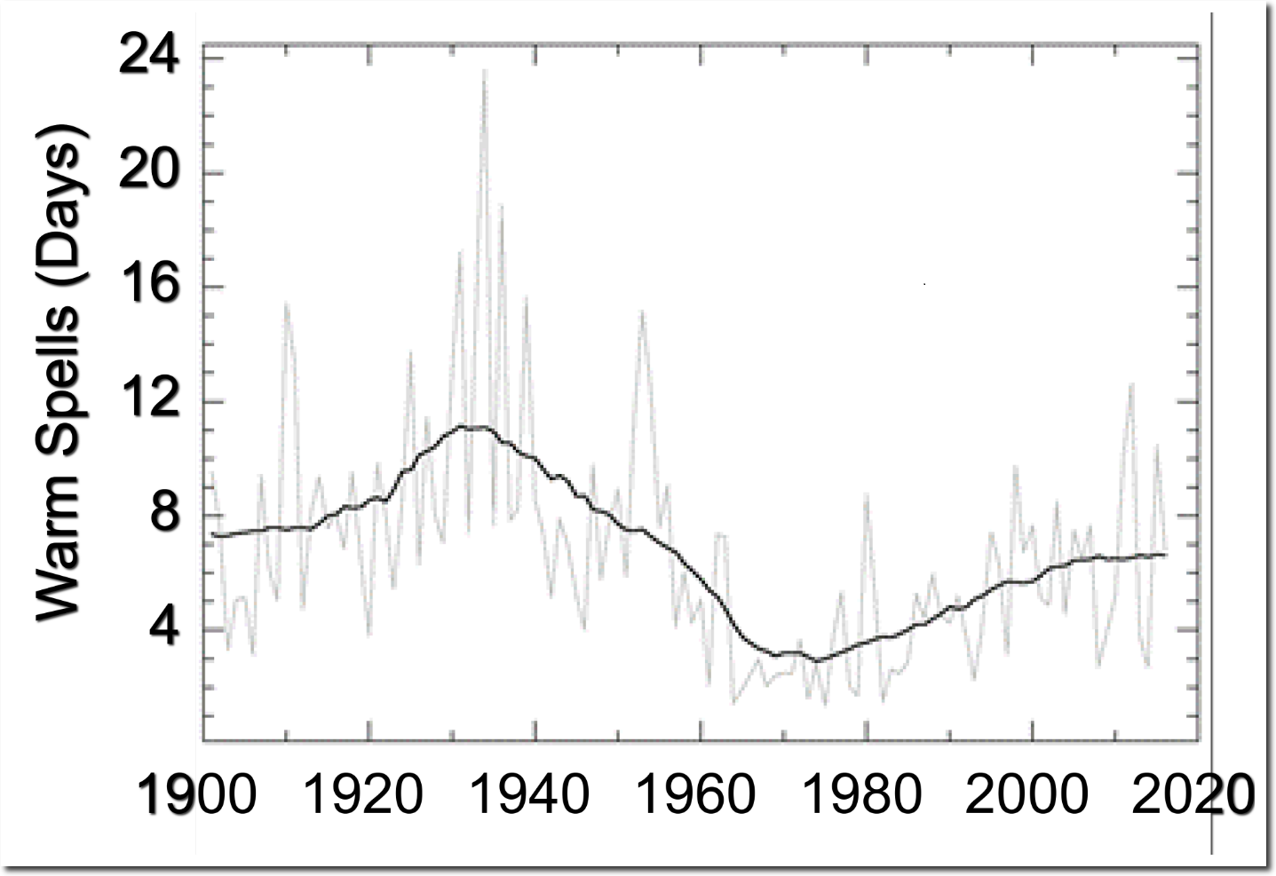
The National Climate Assessment (https://science2017.globalchange.gov/chapter/6/) has the below graph, which shows how much hotter the US used to be.
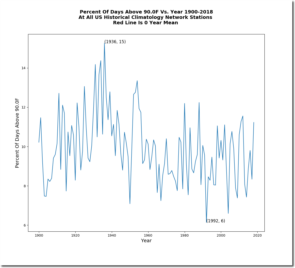
I will set out a couple of more of hiss plots (but read the article for more detail).
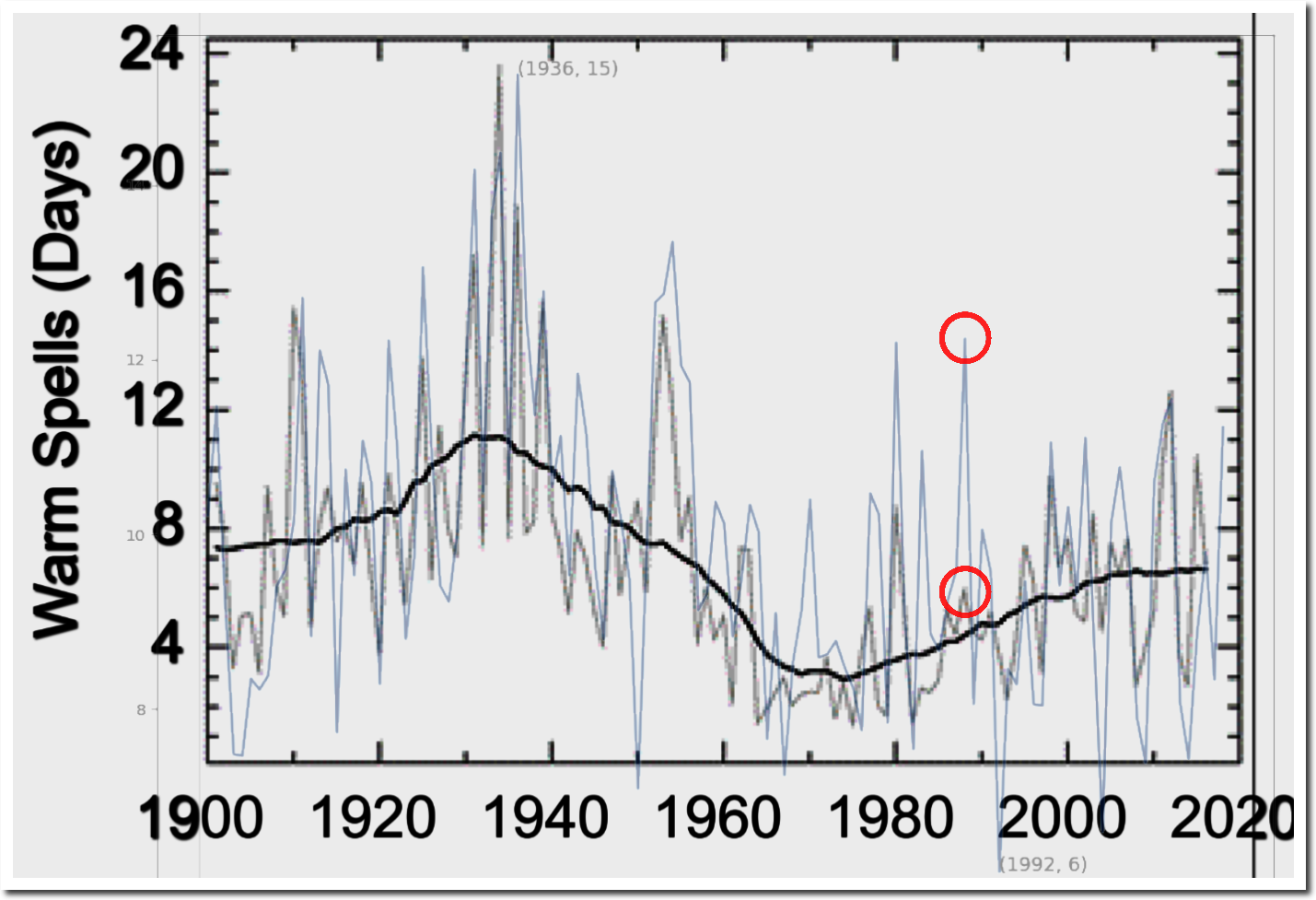
And to show the impact of adjustmenst:
The truth of the matter is that we have no idea as to the temperature of the planet such that all we can say is that it has warmed since the depth of the the LIA and that there are large amounts of multidecadal variation but we do not know whether the planet today is any warmer than it was in the 1940s, or for that matter the 1980s.
Thermometers aren’t scary enough.
That said, there is a scientific basis for using anomalies rather than absolute temperature values. It’s the best way to evaluate tiny variations in a highly variable time series, with a baseline 15 to 30 times the size of the anomalies. It’s similar to the rationale for logarithmic scales.
However, the Climatariat clearly do it to make a minuscule number look very big. If geology was done by the Climatariat, no photos would ever include a lens cap for scale… 😎
I had desired to post something much more detailed but if one sets out a number of citations then the comment is chucked into moderation.
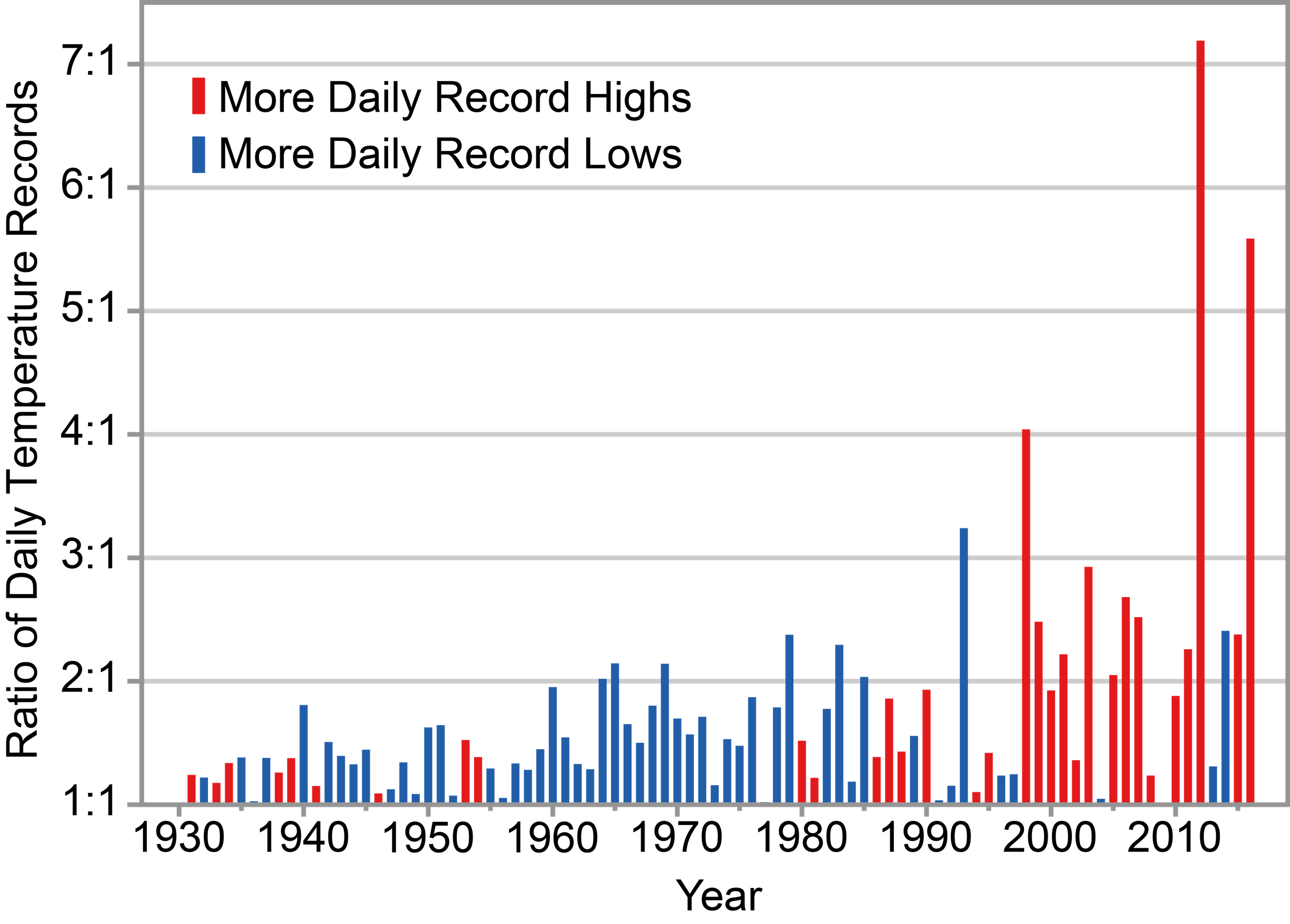
It is well worth having a look at the recent National Climate Assessment Report, and in particular Chapter 6.1.2 Temperature Extremes. I will set out some of their plots which demonstrate the misuse of statistics.
See figure 6.4:
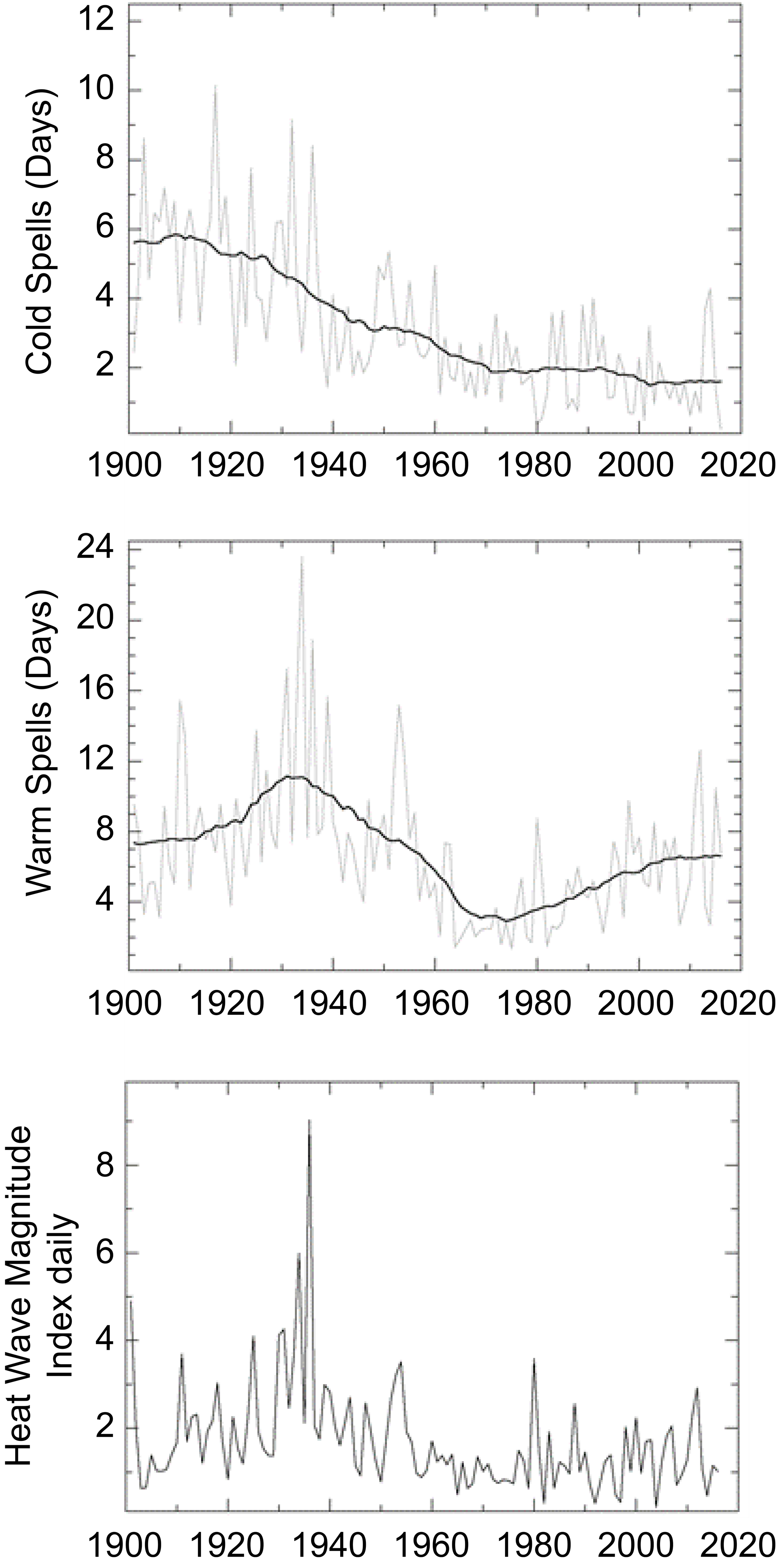
Note the large number of warm days and hot spells in the 1930s, and also the large number of cold days in the 1930s.
Now look at how they combine this data (in figure 6.5) to show the number of extremes to give the impression that extremes were very minimal in the 1930s and the climate is far more extreme today:
Tony Heller has done a very good video discussing the extremes of 1936.
Thanks, Kip.
You made my day.
I don’t wish to put words into Gavin’s mouth but I’m pretty certain that he’d say that if the uncertainty was wider, it’d mean that things could be worse than we thought. He does, after all, like to look on the gloomy side.
Good work Kip, I enjoy your writing particularly.
I’ve long be struck by the fact that the reason given in Meteorology for the use of anomalies is that they provide more useful information about a particular place – against the background of its local climate – than absolute temperature, which does not indicate that information directly.
That this “usefulness” now extends to the globe* has always seemed a rather anomalous usage to me! 😉
*The use of local anomalies from vastly different climates to calculate a single global temperature.
“reducing the uncertainty of annual Global Average Surface Temperatures by a whole order of magnitude”
Well, we’ve been through all that before. Yes, if you subtract the variable that incorporates most of the uncertainty (location/seasonal mean), you know the remainder much better.
But there is a clear contradiction in the broad fuzz that is supposed to be the alternative fact. Expected variability actually means something. It means that you expect to see randomness of that amplitude. And you simply don’t see it. It isn’t there. There is nothing like variability of the order of ±0.5°C (sd). The graph is self-disproving.
Why poor Pluto? If he had not kidnapped Proserpine and fed her pomegranates there would be no winter, just balmy comfortable temperatures and continuously growing crops. I feel it is Pluto we have to blame for all of our problems.
/grins
It seems that most scientists think that if you average enough samples, you will reduce uncertainty and get a more accurate result.
It’s common to call our measurements the signal and to call the errors noise. If the errors are truly random then the assumption, that averaging reduces uncertainty, is correct. One of my favorite demonstrations is to extract a small signal from data where the noise is a hundred times as strong as the signal. It’s a powerful technique.
The problem comes when the noise is not truly random. Then we can have red noise. If you play red noise and random noise over a speaker you can hear the difference. The red noise has more low frequencies and fewer high frequencies.
Natural processes tend to produce red noise. Averaging does not reduce uncertainty where there is red noise. link
I’m not a statistician but I have lots of experience processing signals. I strongly suspect that the uncertainty of the global temperature is understated. The idea that any kind of processing can reduce that uncertainty doesn’t pass the smell test.
Just as James Hansen, with no rigorous mathematical justification, threw Bode feedback analysis at climate sensitivity, it seems that climate scientists have done the same with averaging. In both cases the method is unjustified. There should be a rule that, where statistics is invoked, a statistician should be involved.
Kip,
Excellent.
Just a retired engjneer and amateur astronomer but my confidence in the minuscule star wobbles in defining the very existence of a planet and ‘habitable zones’ definitions is low. Too many other variables effect habitability; stellar eruptions, solar wind, planet rotation, magnetic field, atmosphere and its density and composition and on and on. Most of the “earthlike” planet hype is just that, hype. But the actual search is great for expanding science. Much too much certainty is implied, however, in most of the hype.
Christy and Spencer report UAH results as anomalies as well. How does that figure into this analysis?
I made a very similar case in my papers examining uncertainty due to systematic measurement error in the global air temperature record, here (900 kb pdf), and here (1 mb pdf).
Everyone in the field, GISS, UKMet/UEA, BEST, and RSS and even UA Huntsville for the satellite temps, assume measurement error is a constant that subtracts away in an anomaly.
That assumption is untested and unverified. As you directly imply, Kip, the entire field rests on false precision.
Regarding the phrase “life-as-we-know-it” that was implicitly tied into the thermometer graphic and specified temperatures in this article, here is the range of temperatures that life on Earth has demonstrated (based on current human knowledge):
“. . . another group of scientists has found a microbe from deep-sea vents that is able to survive at 122C. And there are hints that even this is not the ultimate limit for life. A new microbe, for now called “Strain 121”, has since been discovered in a thermal vent deep in the Pacific Ocean. The microbe thrives at 121C and there are claims that it can even survive for two hours at 130C. However the finding is still contentious, as the strain has not been made publicly available to study.” — source http://www.bbc.com/earth/story/20160209-this-is-how-to-survive-if-you-spend-your-life-in-boilin-water
“The study, published in PLoS One, reveals that below -20 °C, single-celled organisms dehydrate, sending them into a vitrified – glass-like – state during which they are unable to complete their life cycle. The researchers propose that, since the organisms cannot reproduce below this temperature, -20 °C is the lowest temperature limit for life on Earth. Scientists placed single-celled organisms in a watery medium, and lowered the temperature. As the temperature fell, the medium started to turn into ice and as the ice crystals grew, the water inside the organisms seeped out to form more ice. This left the cells first dehydrated, and then vitrified. Once a cell has vitrified, scientists no longer consider it living as it cannot reproduce, but cells can be brought back to life when temperatures rise again. This vitrification phase is similar to the state plant seeds enter when they dry out. ‘The interesting thing about vitrification is that in general a cell will survive, where it wouldn’t survive freezing, if you freeze internally you die. But if you can do a controlled vitrification you can survive,’ says Professor Andrew Clarke of NERC’s British Antarctic Survey, lead author of the study. ‘Once a cell is vitrified it can continue to survive right down to incredibly low temperatures. It just can’t do much until it warms up. ‘ ” — source https://phys.org/news/2013-08-lowest-temperature-life.html
Worse, we have made only limited near-observations at the edge of our solar system. The signals from outside are limited and the missing information is inferred based on Earth-biased assumptions/assertions.
If the “expanded” error was correct, then the plotted data should be outside the error about 5% of the time. The fact that this relationship does not hold between the original plot and your “corrected” error range shows that something is wrong with the “corrected plot” (the original does appear to follow the rule).
Good post/essay.
Kip:
Would you agree an anomaly is anchored by a base number? If so, how is that defined? I am working on a comment comparing the two things as you did.
Thanks for sharing, I’ve been making the point about absolute temps for years, but never this well.
We’re pretty sure it’s gotten warmer, but we really don’t know a lot beyond that, despite all the claims about “warmest years.”
And plotting model uncertainty against temperature uncertainty, you quickly realize models are not the sharpest policy tool in the shed, and indeed are barely falsifiable in time ranges of interest.
“…transformation of Uncertain Data into Certain Anomalies, reducing the uncertainty of annual Global Average Surface Temperatures by a whole order of magnitude…”
I think you have not highlighted the whole problem. The problem is partly nomenclature and partly not following through with the anomaly calculation.
The uncertainty has two elements: what the actual measurement is and where the centre of the range is. The measurement uncertainty for each individual measurement is fixed by the instrument used. Full stop. That never disappear because it is inherent in the instrument.
Taking a number of measurements of the same thing, conceptualized as making more than one measurement of the same phenomenon in the same circumstances, produces a range of answers. The more one takes, the more data there is to work with. Using say, 30 measurements of the length of a piece of string one can calculate the standard deviation about the mean (average) of all the lengths. With these additional measurements one can say where the average lies admitting there is a NEW uncertainty about that calculation, which is rooted in the number of measurements taken, nothing to do with the uncertainty of each individual measurement.
The point is that GISS shows the uncertainty about where the average lies, the middle of the range, but has not shown the uncertainty propagated from the original measurements, which remains unchanged.
Plotting the anomaly and the uncertainty of each centre-of-range value based on the number of readings taken, has nothing to do with the uncertainty of the measurement value itself – they just left out that part of the sum. The calculation is incomplete.
You can complete the chart by adding the uncertainty bars up and down to the upper and lower limits shown in the anomaly chart.
The error is very typical of work done by learners who take the output of any calculation or estimation as a ‘fact’, and then use it in a new formula. It is like taking model output as data and running it through another model.
Error propagation is well studied. It is impossible that GISS doesn’t know they are leaving out a step. Uncertainty in the measurement values propagates through to the anomaly chart, plus the uncertainty of where the centre of the readings is minus the baseline.
As is, the anomaly chart is a wrong answer. An error, because it incorporates a mistake – a failure to propagate the measurement uncertainty through to the calculated result, whatever that result is – it doesn’t have to be an anomaly chart. Uncertainty ALWAYS increases with additional calculations. Every physicist knows this. GISS is pretending they don’t.
Kip, Excellent, your article re-enforces beliefs I had for a long time as to why the “warmists” use anomalies instead of absolute global mean temperatures. I carried my beliefs over from when I was looking at monthly Sea Surface Temperatures and SST anomalies in studying large marine pelagic fish. I became concerned in the late 1970s when NOAA began to change how they were determining their anomalies. Never did figure out why they changed their methodologies. The only explanation I ever got had to do how satellite data was being used, somehow their “new” methodology was more “accurate” and they were “changing computer systems(?).” Shortly thereafter I moved on to other research so never bothered to follow up any further.
Let us also talk about sea level measurements. How can they give us 1/100mm accuracy if systematic uncertainty is ca. 3-4mm? You can’t do better than your systematic uncertainty. Therefore the satellite sea level measurements are complete BS.