From Dr. Roy Spencer’s Global Warming Blog
by Roy W. Spencer, Ph. D.
The recent devastating floods in western North Carolina were not unprecedented, but were certainly rare. A recent masters thesis examining flood deposits in the banks of the French Broad River over the last 250-300 years found that a flood in 1769 produced water levels approximately as high as those reported in the recent flood from Hurricane Helene. So, yes, the flood was historic.
Like all severe weather events, a superposition of several contributing factors are necessary to make an event “severe”, such as those that led to the NC floods. In that case, a strong hurricane combined with steering currents that would carry the hurricane on a track that would produce a maximum amount of orographic uplift on the east side of the Smoky Mountains was necessary in order to produce the widespread 12-20 inch rainfall amounts, and the steering currents had to be so strong that the hurricane would penetrate far inland with little weakening.
Again, all severe weather events represent the somewhat random combining of amplifying components: In the case of Hurricane Helene, they produced the unlucky massive flooding result that the region had not seen in hundreds of years.
The Random Component of Precipitation Variability
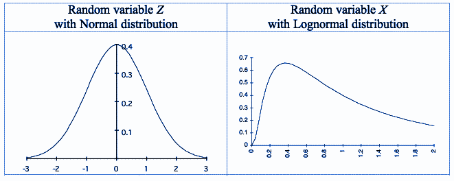
The rare superposition of several rare contributing factors, or the more common superposition of more common factors, can be examined through statistics when one examines many events. For example, it has long been known that precipitation statistics gathered over many years exhibit a log-normal frequency distribution. Simply put, the lowest precipitation amounts are the most frequent, and the highest amounts are the least frequent. This is the statistical result of the superposition of contributing factors, such as (in the case of excessive rainfall) abundant humidity, an unstable air mass, low-level convergence of air, a stationary or slow-moving storm (In western NC, the mountains providing uplift are stationary), etc.
Extreme precipitation events are (of course) the most rare, and as such, they can exhibit somewhat weird behavior. This is why hydrologists disagree over the usefulness of the term “100-year flood”, since most weather records don’t even extend beyond 100 years. One would probably need 1,000 years of rainfall records to get a good estimate of what constitutes a 100-year event.
Simulating Extreme Rainfall Events through Statistics
It is easy in Excel to make a simulated time series of rainfall totals having a log-normal distribution. For example, the following plot of hypothetical daily totals for the period 1900 through 2024 shows an seemingly increasing incidence of days with the heaviest rainfall (red circles). Could this be climate change?

But remember, these are randomly generated numbers. Just like you can flip a coin and sometimes get 4 heads (or 4 tails) in a row doesn’t mean there is some underlying cause for getting the same result several times in a row. If we extend the above plot from 125 years to 500 years, we see (following plot) that there is no long-term increasing trend in heavy rainfall amounts:

Black Swan Events
Or, how about this one, which I will call “The Great Flood of August 28, 2022”?:

Note that this event (generated with just log-normally distributed random numbers) far exceeds any other daily event in that 500-year plot.
The point here is that too often we tend to attribute severe weather events to some underlying cause that is emerging over time, such as global warming. And, I believe, some of the changes we have seen in nature are due to the (weak and largely benign) warming trend most regions of the world have experienced in the last 100 years.
But these events can occur without any underlying long-term change in the climate system. To attribute every change we see to global warming is just silly, especially when it comes to precipitation related events, such as flood… or even drought.
A “Random Drought”
Now changing our daily random log-normal precipitation generator to a monthly time scale, we can look at how precipitation amounts change from decade to decade. Why monthly? Well, weather variations (and even climate cycles) tend to have preferred time scales. Several days for synoptic weather patterns, quasi-monthly for some kinds of persistent weather patterns, and even yearly or decadal for some natural internal climate cycles.
When I generate random log-normal time series at monthly time scales, and compute decadal averages over the last 120 years, seldom is the long-term trend close to zero. Here’s one what shows low precipitation for the most recent three decades, just purely through chance:

That looks like something we could attribute to drought in California, right? Yet, it’s just the result of random numbers.
Or, we can choose one of the random simulations that has an increasing trend:

I’m sure someone could tie that to global warming.
A Final Word About 100-Year Flood Events
There seems to be some misunderstanding about 100-year events. These almost always apply to a specific location. So, you could have 100-year events every year in the U.S., and as long they are in different locations, there is nothing unusual about it. A 100-year flood in western North Carolina this year could be followed by a 100-year flood in eastern North Carolina next year. That doesn’t mean 100-year floods are getting more frequent.
I’m not claiming that all severe weather is due to randomness. Only that there is a huge random component to it, and that’s what makes attribution of any kind of severe weather event to climate change essentially impossible.
Most interesting
Some good points made here. But I wouldn’t recommend a log-normal distribution. It is too heavy-tailed – too likely to give extreme points. The normal distribution has plausibility about its tail behaviour from the central limit theorem about summing random variables. The log normal does not have that. And of course you see that in the extremes here.
I think the right distribution to use would be the Poisson.
Nick,
Are your rankings of distributions based on mathematical fits using factors like skew and kurtosis or some other numerical method with tails fitting, or are they judged by appeal of the shape to the eye, like judging a beauty contest in the good old days when we loved and approved of them?
Given the global importance of understanding the distribution, I would have thought that there were elegant computational ways to classify them concisely, but I confess that I have not followed the action in this regard for some years. I am all for statisticians deriving such elegance and teaching it to amateur stats people like me. Geoff S
Geoff,
No, it is more basic than that. The normal distribution is the central limit, where you add many random variables together. The Poisson is the distribution of random positive events accumulating.
The thing is, you can talk about moments, but they don’t give you the tail behaviour. And you probably can’t observe it either, since by definition it is of rare events. So you are left relying on theory for rare events.
Thanks, Nick.
Are you saying obliquely that statistical analysis using distributions and tails in particular is not useful for understanding rare weather events … or, holy of holies, rare climate change events?
Geoff S
Not very obliquely. Distributions are fitted, usually via moments. You won’t have enough data to fit to the tail. So you have to reason that as best you can. It isn’t easy, but it matters.
Accumulating over a given period of time, not just continual accumulation. As the article points out, it should also be based on location. A record in one location may not be a record in another a short distance away.
Your comment is interesting but I am not a statistician (nor i expect are a lot of readers). This looks like a nice discussion between you and Dr. Spencer, but if it is relatively easy to do, why don’t you post a graph or two with whichever distribution you think best so us non-experts can get an idea of what you are talking about.
As an EE who has to do noise analysis every now and then, the normal distribution does not model 1/f noise, which shows up in the datasheet of almost every op amp. The exceptions are chopper stabilized amplifiers.
One point Roy did make is that we don’t have enough data on weather to truly define a “100 year event let alone a “1,000 year event”.
1/f noise
=======
a coin toss has a fixed average and variance. This describes games of chance.
Most people know about average but not variance. Variance measure the distance the data varies from the average.
The greater the variance the greater the likely error.
Time series data like weather or the stock market typically does not have a fixed variance or average, making it inherently unpredictable with unpredictable error.
“One point Roy did make is that we don’t have enough data on weather to truly define a “100 year event let alone a “1,000 year event”.”
I actually agree with that point. You can’t do it empirically, so you have to rely on theory. There is, FWIW, theory associated with the normal and Poisson distributions.
The 1/f noise is a consequence of RC filtering with exponential decay, rather than the accumulation of random events.
People are misled over the statistics because sampling brings the Central Limit Theorem into play. This makes weather and climate data appear normally distributed when in fact it is not.
Nick, I applaude your mention of the central limit theorem because it is key to understanding where climate science has fundamentally gone off the rails. However the CLT does not change the distribution of rainfall. It changes the distribution of collected data according to how the rainfall is sampled.
You are correct with “going off the rails”. The CLT requires one to withdraw samples from the same population in order to be meaningful. Defining the population is paramount. What is the sample size when trending? Climate science just cherry picks things but doesn’t seem capable of properly defining the whole sequence from start to finish.
Example – There are 28, 29, 30, or 31 days in a month at any given station. There are 28, 29, 30, or 31 Tmax value quantities for a month at a given station. Are those a population or a sample? If they are samples, how many Tmax’s actually exist in a month? If they are a population, what does dividing by the √n tell one about an estimated mean?
“It changes the distribution of collected data according to how the rainfall is sampled.”
And that is the data we have.
Perhaps you skipped over this bit of information – “it has long been known that precipitation statistics gathered over many years exhibit a log-normal frequency distribution”
Poisson might be ok for air crashes and deaths in the Prussian army by horse kicks.
How are you going to calculate the mean to incorporate e.g. in about 926 it was so cold both the Nile and the Black Sea froze; in 137 BC it was so hot the Roman armies were forced to march by night; in 1800 BC the Egyptian Pharoah was overthrown because climate change caused the Nile floods to fail?
I agree with your comment about the use of the log-normal distribution. In fact Roy’s description of it is misleading to those who are not familiar with it: “For example, it has long been known that precipitation statistics gathered over many years exhibit a log-normal frequency distribution. Simply put, the lowest precipitation amounts are the most frequent, and the highest amounts are the least frequent.” Actually the log-normal is only appropriate for non-zero, positive numbers, the daily graph produced therefore has no days without rain! You’d need a different model to determine the distribution of days without rain. This summer in NJ has been very dry, the last time it rained was August 18th.
Here’s an example of a log-normal compared with a normal, as Nick said I think it tends to have too long a tail.
Weather ‘experts’ in NZ don’t seem to have too much trouble attributing bad weather to “Climate Change!”.
https://niwa.co.nz/news/cyclone-gabrielle-was-intensified-human-induced-global-warming
They didn’t go so far as to say it was caused by CC, but seem confident about how much worse it was because of it.
Our Prime Minister was in no doubt that this cyclone was caused by CC, just days after it struck…
https://www.1news.co.nz/2023/02/15/no-doubt-cyclone-gabrielle-a-result-of-climate-change-luxon/
I wonder who advised him about this…
Luxon goes with what he thinks voters want to hear
Reports from staff at Air New Zealand indicates that he follows whims and changes is mind often . Like most places NZ politics is full of ignorant vote chasers that have drunk plenty off cool aid
“this cyclone was caused by [Climate Change] ”
Or equally, “this cyclone was weather change”.
What is the distinction between climate change and weather change?
One is real and one isn’t?
Right Phil.
As much as everyone talks about the weather, I’ve never encountered a Weather Denier.
“Climate” has been redefined by the UN/WMO to be 30 years of weather now.
Assuming there are no identical tying values for given years, if you have a ten year period of record, the odds of any year being the record year for anything is one in ten. For a hundred year POR, it would be one in a hundred. For a 500 year POR, it would be 1/500…and so on. The longer the period of record, the less likely it is that any given year will break an all-time record, however, the longer your period of record lasts, the likelier it is that eventually new records will be set. It’s just a matter of time. No trends or external forcings are required.
Yet a trend clearly exists.
Take Roy Spencer’s own UAH_TLT data set. This will have 46 years of full annual data by December this year, yet 9 out of its 10 warmest years on record have occurred in the past 14 years. Three of the four warmest years have occurred since 2000 (2024 will surpass 2023 as the new record warmest year in UAH, barring a climatic catastrophe of some sort between now and the end of the year).
With a sample size of 46, the chances of the three warmest years all occurring in such close proximity are vanishingly small. However, it is entirely consistent with the theory that global temperatures are rising over time.
Three of the four warmest years have occurred since 2020, sorry, not 2000.
And what happened for the 46 years before UAH-TLT, or the 46 years before that?
You miss the entire point. Why do you think you might get 5 or even 10 heads in a row from flipping a coin? If you flip a coin 50 times (50 years) would you expect some number of heads in a row (or tails) to appear during that time? Dr. Spencer has tried to show you that things like records can occur randomly without a trend. Looking back 100 years or 500 years, or even 1000 years, can you say that the records you are positing are unprecedented in all of history or are they just happening at random?
I think you could have stopped right there. 🙂
Looking at individual years is just a handy concept for us to use. Why not use decades, centuries, or individual days or weeks? If a given decade happens to be quite warm, for whatever reason, then yes, I’d expect a string of years in that decade to be warm.
1) A trend for temperature exists, not for Extreme weather.
2) The general trend for temperature has been positive since the end of the 17th century (the bottom of the Little Ice Age), long before any significant human effect on CO2 levels.
3) The upward trend is less than half of the rate predicted by the theory that humans are the primary cause of temperature rise.
I love your site and your point of view. And you are right, the weather appears random – certainly not directed by CO2 or the like. As a scientist, however, nothing is random. Einstein was right, Heisenberg remains wrong. The proof that there is no randomness at the quantum level lies, indirectly, in the fact that when all those results at the quantum level are integrated, the result is the non-random laws at the macro level.
Indirectly = proof?
If it were indeed random, then the mathematical integration of the sets of measurement at the quantum level would also be random. Instead, the integration of the results coincides with the non-random macro law. So while this is not direct proof, i.e., no direct measurement, that quantum mechanics is not random, it does, indirectly prove it
Supports the hypothesis. That is different than proof.
Definitions, definitions. I said indirect proof. Explain how the integral could be non-random when the alleged results are random. I say alleged results because the data, in my opinion, is from faulty testing
A scientist speaking here to those open to scientific arguments and debate i.e. the importance of evidence.
I wonder how easy the learned author would find it to convince ‘public representatives’ on Capitol Hill and in the White House; MSM ‘anchors’ who prostitute themselves for money; gormless footsoldiers of the Democrat party; or HEI grant-seekers who will lose their jobs if they don’t keep spinning the ‘climate chaos’ dictum??
‘In a world where lying is necessary to keep your job and the ambitious have to lie as a matter of survival, telling the truth is limited to the mavericks, the unemployed, the retired still with critical faculties and those for whom pissing off the Establishment is a daily source of frisson’.
I am afraid that the two groups that you have defined, “those open to scientific arguments and debate i.e. the importance of evidence” and “‘public representatives’ on Capitol Hill and in the White House; MSM ‘anchors’, et al, are mutually exclusive.
Brings to mind the Pauli Exclusion….
Roy,
Here are some daily and monthly record rainfall numbers for each month of the year at the little town of Tully, North Queensland, about 17.61°S, 146.0°E 19m AMSL, record-keeping commenced 1920.
The underscore several of your interesting observations. For example, the month with the highest daily rain is not the month with the highest monthly rain. And more.
Highest daily rainfall on record.
Jan 30 2010 4.9 inches of rain in the day
Feb 5 2011 4.6 inches
Mar 4 1954 10.4 inches
April 23 1950 9.3
May 27 2007 12.2
June 9 2017 18.1
July 4 2011 15.7
Aug 6 2018 27.6 inches in the day, the highest on Tully record
Sept 21 2003 12.5
Oct 7 1964 8.1
Nov 22 1921 6.2
Dec 1 2021 4.8 inches in the day.
Highest monthly rainfall on record.
High Rain (mm) High Rain (inches)
Jan, 1959 414.3 16.3
Feb, 1998 393 15.4
Mar, 1930 431.1 16.9
Apr, 2000 804 31.6
May, 1973 1048.7 41.2
June, 1981 2748.6 108.0
July, 1977 1496.7 58.8
Aug, 1921 1576.9 62.0
Sept, 2021 1203.8 47.3
Oct, 1964 825.4 32.4
Nov, 1957 503.2 19.8
Dec, 1969 442.6 17.4
Here in Australia, where the expression was “Call that a knife?” we might now say of eastern US “Call that heavy rain?”
Geoff S
All rivers flood- which is why there are flood plains. Don’t build in the flood plain unless engineers have solved what to do with the flood waters when it happens. Like, dam up all the streams. But of course the enviros/greens hate dams. Then instead of whining about cc causing big floods, they should promote not building in flood plains and support superior engineering of the river system.
Where’s the money (aka 10%) in that?
A lack of understanding statistics is why casinos prosper.
This is known as “observation bias” or “sampling bias.” In this case, the perceived change is due to the varying length or conditions of observation rather than any real change in the underlying data. A specific form of this, when changes are mistakenly attributed to time, is called the “time-window effect” or “duration bias.”
Fred,
I give a rainfall example of observation bias in the town of Tully, Queensland, further down in comments. Check the difference in timing between daily and monthly records.
Also, this set of numbers seems to indicate that rainfall DAILY records seem to have increased past year 2000, while no such trend appears in MONTHLY records from the same place.
You can take many types of record through stats or eyeball analysis and deduce quite the wrong outcome.
Roy is just so correct to show some effects of random timing in Nature. I am adding to the examples.
Geoff S
If you watch the ocean day after day you will on occasion see waves taller than any previous. The waves are not getting taller. What is changing is the length of observation.
Climate Chane is not real change. It is a statistical effect of changing the length of observation.
Mostly true. However, one can not so easily dismiss that the climate today has changed from the climate 1 million years ago or 5 billion.
Climate change is a coin toss ending in HHHH. It is statistically just as likely as TTTT or THTH.
It is very difficult statistically to prove climate change is not simply due to chance.
Climate Science uses 2 standard deviations as its standard of proof. Statistically this is garbage. It proves nothing.
If engineers used 2 standard deviation as their standard of proof you would have a 5% chance of dying every time you rode an elevator.
Most climate and weather data is stored on computers as the average of averages. Rarely is raw data stored or used because of the cost and time required to process.
What is largely ignored is that this averaging process fundamentally changes the data statistically. It reduces the variance which makes the statistical error appear much smaller than it actually is.
As a result you have the IPCC and climate scientists in general proclaiming with high certainty that such and such is likely when all they are really doing is quoting false statistics.
Aside from a few climate scientists like Judith Curry it appears most are not aware of this problem and as a result do not maintain the degree of skepticism required for healthy scientific discovery.
Anomalies are the perfect example. They are calculated by subtracting the means of two random variables. When this is done, the variances add! NIST TN1900 Ex. 2 calculates an expanded standard uncertainty of the mean of ±1.8°C. Even if the 30 year baseline average had ±0°C uncertainty, the subsequent anomaly would have the ±1.8°C uncertainty. Where does this uncertainty disappear to? THE TRASH CAN!
“There seems to be some misunderstanding about 100-year events. These almost always apply to a specific location.”
My understanding of the term “(fill in the blank) year flood” was a term used by those in the profession that they understood NOT to mean “once in (fill in the blank) years” but more along the lines of the odds that that location might experience such a flood?
Sort of like an engine rated 100 “horse power” does not mean that 100 horses could reach 0-60 in 1 minute.
The term “(fill in the blank) year flood” has been taken more literally than intended.
It is true that a specified storm including its frequency is specific to a particular location using data from that location … so that in between locations that actually have a usable data record one can interpolate. Also, the probabilistic data contour curves that are overlaid on a map are regional and do not represent very small watersheds that can have extreme values that do not necessarily characterize the values in surrounding larger watersheds.
Think of it this way – the weather forecasters may predict 1 inch of rainfall on a day in a given city or county that is representative of that area. But if a particular rain gage is at the exact location where a thunderstorm releases its peak rainfall, the resulting measured rainfall depth can be much higher than the predicted depth for the larger area.
It is a probabilistic term, not a trend. It means that in the next one hundred years one can expect a repeat at that location. That could happen tomorrow or any other time in the next one hundred years, and it resets each time it occurs.
The mayor or NYC when faced with 2 consecutive years of 100-year storms claimed climate change.
He, of course, was wrong. Weather merely beat the 1 in 100 odds of a storm of that magnitude occurring in any given year.
No – this analysis is incorrect. One can deduce the probability of certain events taking place, including improbable events, without having a historical record equaling the return period. It’s done through quite normal acceptable unbiased probability analysis. The probability analysis considers the length of the record, the variability in the data, and the two-tailed normal distribution used pretty much everywhere in probability analysis, and from that process hydrologists and engineers generate a probabilistic estimate of variability.
Don’t confuse this with a prediction.
And the meaning of a 100 year storm is not that it can only occur once every 100 years, but rather, that on average such a storm will occur once every 100 years. But this allows that one can get 100 year events on successive days, months, or even years due to the normal variability in weather patterns where there are wet years and dry years that vary year to year, decade to decade, century to century, millennium to milennium, and so forth up to cycles millions of years long.
If engineers could not generate 100 year probabilistic estimates of rainfall and flood elevation from less than 100 years of data, then by the author’s statement they could never provide an estimate for what is now standard flood risk protection …because few reporting stations have 100 years of data. Data used in the analysis must be at least 30 years in length – keeping in mind that is data for rainfall depth, duration of the storm for 365 days per year. That’s a heckuva lot of data to crunch for even the minimum record.
Also, do not confuse return period with any kind of proportional relationship, because of the two tailed normal distribution. The 100 year rainfall depth event is not 10 times the 10 year event. The rainfall depths tend to follow a logarithmic relationship where, for example, depending upon the actual data at a given location, the 100 year event may be only 30-40% higher than the 10 year event, and the 500 year event may be only 10% greater than the 100 year event. The probability curves always flatten out.
Can I please recommend that this article from Dr Spencer becomes more interesting if you read and understand the statistical work on historic Nile River levels by Hurst and Kolmogorov, with the following link as a start point.
It is a fascinating story. Geoff S
This is way over my head and I’m not going to pretend I understand it, but in skimming through it two general statements stood out to me. I fully admit that they are (or may be) taken out of context and may not mean exactly what i think they mean, but:
and,
I found this to be interesting.
For the earth to have a temperature range from say, 40°C to -50°C on any given day, an average ‘global’ temperature just hides so much variability when accompanied by a standard uncertainty of the mean rather than a standard uncertainty (of the dispersion of data attributed to the mean). This contributes to propaganda efforts but little to scientific understanding.
I think it was a good reference from sherro01. I hope more people read it and understand it (better than I do). I downloaded it and need to try to work my way through it.