By Greg Chapman
“The world has less than a decade to change course to avoid irreversible ecological catastrophe, the UN warned today.” The Guardian Nov 28 2007
“It’s tough to make predictions, especially about the future.” Yogi Berra
Introduction
Global extinction due to global warming has been predicted more times than climate activist, Leo DiCaprio, has traveled by private jet. But where do these predictions come from? If you thought it was just calculated from the simple, well known relationship between CO2 and solar energy spectrum absorption, you would only expect to see about 0.5o C increase from pre-industrial temperatures as a result of CO2 doubling, due to the logarithmic nature of the relationship.

The runaway 3-6o C and higher temperature increase model predictions depend on coupled feedbacks from many other factors, including water vapour (the most important greenhouse gas), albedo (the proportion of energy reflected from the surface – e.g. more/less ice or clouds, more/less reflection) and aerosols, just to mention a few, which theoretically may amplify the small incremental CO2 heating effect. Because of the complexity of these interrelationships, the only way to make predictions is with climate models because they can’t be directly calculated.
The purpose of this article is to explain to the non-expert, how climate models work, rather than a focus on the issues underlying the actual climate science, since the models are the primary ‘evidence’ used by those claiming a climate crisis. The first problem, of course, is no model forecast is evidence of anything. It’s just a forecast, so it’s important to understand how the forecasts are made, the assumptions behind them and their reliability.
How do Climate Models Work?
In order to represent the earth in a computer model, a grid of cells is constructed from the bottom of the ocean to the top of the atmosphere. Within each cell, the component properties, such as temperature, pressure, solids, liquids and vapour, are uniform.
The size of the cells varies between models and within models. Ideally, they should be as small as possible as properties vary continuously in the real world, but the resolution is constrained by computing power. Typically, the cell area is around 100×100 km2 even though there is considerable atmospheric variation over such distances, requiring each of the physical properties within the cell to be averaged to a single value. This introduces an unavoidable error into the models even before they start to run.
The number of cells in a model varies, but the typical order of magnitude is around 2 million.

Once the grid has been constructed, the component properties of each these cells must be determined. There aren’t, of course, 2 million data stations in the atmosphere and ocean. The current number of data points is around 10,000 (ground weather stations, balloons and ocean buoys), plus we have satellite data since 1978, but historically the coverage is poor. As a result, when initialising a climate model starting 150 years ago, there is almost no data available for most of the land surface, poles and oceans, and nothing above the surface or in the ocean depths. This should be understood to be a major concern.

Once initialised, the model goes through a series of timesteps. At each step, for each cell, the properties of the adjacent cells are compared. If one such cell is at a higher pressure, fluid will flow from that cell to the next. If it is at higher temperature, it warms the next cell (whilst cooling itself). This might cause ice to melt or water to evaporate, but evaporation has a cooling effect. If polar ice melts, there is less energy reflected that causes further heating. Aerosols in the cell can result in heating or cooling and an increase or decrease in precipitation, depending on the type.
Increased precipitation can increase plant growth as does increased CO2. This will change the albedo of the surface as well as the humidity. Higher temperatures cause greater evaporation from oceans which cools the oceans and increases cloud cover. Climate models can’t model clouds due to the low resolution of the grid, and whether clouds increase surface temperature or reduce it, depends on the type of cloud.
It’s complicated! Of course, this all happens in 3 dimensions and to every cell resulting in considerable feedback to be calculated at each timestep.
The timesteps can be as short as half an hour. Remember, the terminator, the point at which day turns into night, travels across the earth’s surface at about 1700 km/hr at the equator, so even half hourly timesteps introduce further error into the calculation, but again, computing power is a constraint.
While the changes in temperatures and pressures between cells are calculated according to the laws of thermodynamics and fluid mechanics, many other changes aren’t calculated. They rely on parameterisation. For example, the albedo forcing varies from icecaps to Amazon jungle to Sahara desert to oceans to cloud cover and all the reflectivity types in between. These properties are just assigned and their impacts on other properties are determined from lookup tables, not calculated. Parameterisation is also used for cloud and aerosol impacts on temperature and precipitation. Any important factor that occurs on a subgrid scale, such as storms and ocean eddy currents must also be parameterised with an averaged impact used for the whole grid cell. Whilst the effects of these factors are based on observations, the parameterisation is far more a qualitative rather than a quantitative process, and often described by modelers themselves as an art, that introduces further error. Direct measurement of these effects and how they are coupled to other factors is extremely difficult and poorly understood.
Within the atmosphere in particular, there can be sharp boundary layers that cause the models to crash. These sharp variations have to be smoothed.
Energy transfers between atmosphere and ocean are also problematic. The most energetic heat transfers occur at subgrid scales that must be averaged over much larger areas.
Cloud formation depends on processes at the millimeter level and are just impossible to model. Clouds can both warm as well as cool. Any warming increases evaporation (that cools the surface) resulting in an increase in cloud particulates. Aerosols also affect cloud formation at a micro level. All these effects must be averaged in the models.
When the grid approximations are combined with every timestep, further errors are introduced and with half hour timesteps over 150 years, that’s over 2.6 million timesteps! Unfortunately, these errors aren’t self-correcting. Instead this numerical dispersion accumulates over the model run, but there is a technique that climate modelers use to overcome this, which I describe shortly.

Model Initialisation
After the construction of any type of computer model, there is an initalisation process whereby the model is checked to see whether the starting values in each of the cells are physically consistent with one another. For example, if you are modelling a bridge to see whether the design will withstand high winds and earthquakes, you make sure that before you impose any external forces onto the model structure other than gravity, that it meets all the expected stresses and strains of a static structure. Afterall, if the initial conditions of your model are incorrect, how can you rely on it to predict what will happen when external forces are imposed in the model?
Fortunately, for most computer models, the properties of the components are quite well known and the initial condition is static, the only external force being gravity. If your bridge doesn’t stay up on initialisation, there is something seriously wrong with either your model or design!
With climate models, we have two problems with initialisation. Firstly, as previously mentioned, we have very little data for time zero, whenever we chose that to be. Secondly, at time zero, the model is not in a static steady state as is the case for pretty much every other computer model that has been developed. At time zero, there could be a blizzard in Siberia, a typhoon in Japan, monsoons in Mumbai and a heatwave in southern Australia, not to mention the odd volcanic explosion, which could all be gone in a day or so.
There is never a steady state point in time for the climate, so it’s impossible to validate climate models on initialisation.
The best climate modelers can hope for is that their bright shiny new model doesn’t crash in the first few timesteps.
The climate system is chaotic which essentially means any model will be a poor predictor of the future – you can’t even make a model of a lottery ball machine (which is a comparatively a much simpler and smaller interacting system) and use it to predict the outcome of the next draw.
So, if climate models are populated with little more than educated guesses instead of actual observational data at time zero, and errors accumulate with every timestep, how do climate modelers address this problem?
History matching
If the system that’s being computer modelled has been in operation for some time, you can use that data to tune the model and then start the forecast before that period finishes to see how well it matches before making predictions. Unlike other computer modelers, climate modelers call this ‘hindcasting’ because it doesn’t sound like they are manipulating the model parameters to fit the data.
The theory is, that even though climate model construction has many flaws, such as large grid sizes, patchy data of dubious quality in the early years, and poorly understood physical phenomena driving the climate that has been parameterised, that you can tune the model during hindcasting within parameter uncertainties to overcome all these deficiencies.
While it’s true that you can tune the model to get a reasonable match with at least some components of history, the match isn’t unique.
When computer models were first being used last century, the famous mathematician, John Von Neumann, said:
“with four parameters I can fit an elephant, with five I can make him wiggle his trunk”
In climate models there are hundreds of parameters that can be tuned to match history. What this means is there is an almost infinite number of ways to achieve a match. Yes, many of these are non-physical and are discarded, but there is no unique solution as the uncertainty on many of the parameters is large and as long as you tune within the uncertainty limits, innumerable matches can still be found.
An additional flaw in the history matching process is the length of some of the natural cycles. For example, ocean circulation takes place over hundreds of years, and we don’t even have 100 years of data with which to match it.
In addition, it’s difficult to history match to all climate variables. While global average surface temperature is the primary objective of the history matching process, other data, such a tropospheric temperatures, regional temperatures and precipitation, diurnal minimums and maximums are poorly matched.
Even so, can the history matching of the primary variable, average global surface temperature, constrain the accumulating errors that inevitably occur with each model timestep?
Forecasting
Consider a shotgun. When the trigger is pulled, the pellets from the cartridge travel down the barrel, but there is also lateral movement of the pellets. The purpose of the shotgun barrel is to dampen the lateral movements and to narrow the spread when the pellets leave the barrel. It’s well known that shotguns have limited accuracy over long distances and there will be a shot pattern that grows with distance. The history match period for a climate model is like the barrel of the shotgun. So what happens when the model moves from matching to forecasting mode?

Like the shotgun pellets leaving the barrel, numerical dispersion takes over in the forecasting phase. Each of the 73 models in Figure 5 has been history matched, but outside the constraints of the matching period, they quickly diverge.
Now at most only one of these models can be correct, but more likely, none of them are. If this was a real scientific process, the hottest two thirds of the models would be rejected by the International Panel for Climate Change (IPCC), and further study focused on the models closest to the observations. But they don’t do that for a number of reasons.
Firstly, if they reject most of the models, there would be outrage amongst the climate scientist community, especially from the rejected teams due to their subsequent loss of funding. More importantly, the so called 97% consensus would instantly evaporate.
Secondly, once the hottest models were rejected, the forecast for 2100 would be about 1.5o C increase (due predominately to natural warming) and there would be no panic, and the gravy train would end.
So how should the IPPC reconcile this wide range of forecasts?
Imagine you wanted to know the value of bitcoin 10 years from now so you can make an investment decision today. You could consult an economist, but we all know how useless their predictions are. So instead, you consult an astrologer, but you worry whether you should bet all your money on a single prediction. Just to be safe, you consult 100 astrologers, but they give you a very wide range of predictions. Well, what should you do now? You could do what the IPCC does, and just average all the predictions.
You can’t improve the accuracy of garbage by averaging it.
An Alternative Approach
Climate modelers claim that a history match isn’t possible without including CO2 forcing. This is may be true using the approach described here with its many approximations, and only tuning the model to a single benchmark (surface temperature) and ignoring deviations from others (such as tropospheric temperature), but analytic (as opposed to numeric) models have achieved matches without CO2 forcing. These are models, based purely on historic climate cycles that identify the harmonics using a mathematical technique of signal analysis, which deconstructs long and short term natural cycles of different periods and amplitudes without considering changes in CO2 concentration.
In Figure 6, a comparison is made between the IPCC predictions and a prediction from just one analytic harmonic model that doesn’t depend on CO2 warming. A match to history can be achieved through harmonic analysis and provides a much more conservative prediction that correctly forecasts the current pause in temperature increase, unlike the IPCC models. The purpose of this example isn’t to claim that this model is more accurate, it’s just another model, but to dispel the myth that there is no way history can be explained without anthropogenic CO2 forcing and to show that it’s possible to explain the changes in temperature with natural variation as the predominant driver.

In summary:
- Climate models can’t be validated on initiatialisation due to lack of data and a chaotic initial state.
- Model resolutions are too low to represent many climate factors.
- Many of the forcing factors are parameterised as they can’t be calculated by the models.
- Uncertainties in the parameterisation process mean that there is no unique solution to the history matching.
- Numerical dispersion beyond the history matching phase results in a large divergence in the models.
- The IPCC refuses to discard models that don’t match the observed data in the prediction phase – which is almost all of them.
The question now is, do you have the confidence to invest trillions of dollars and reduce standards of living for billions of people, to stop climate model predicted global warming or should we just adapt to the natural changes as we always have?
Greg Chapman is a former (non-climate) computer modeler.
Footnotes
[2] https://serc.carleton.edu/eet/envisioningclimatechange/part_2.html
[3] https://climateaudit.org/2008/02/10/historical-station-distribution/
[4] http://www.atmo.arizona.edu/students/courselinks/fall16/atmo336/lectures/sec6/weather_forecast.html
Whilst climate models are tuned to surface temperatures, they predict a tropospheric hotspot that doesn’t exist. This on its own should invalidate the models.
From the article: “While it’s true that you can tune the model to get a reasonable match with at least some components of history,”
The problem with hindcasting is they are tuning the model to bogus, bastardized climate history.
If your computer model matches a bogus temperature history, what does that say about your computer model. To me that says your computer model is junk as far as forcasting history or the future.
“As a result, when initialising a climate model starting 150 years ago, there is almost no data available for most of the land surface, poles and oceans, and nothing above the surface or in the ocean depths. This should be understood to be a major concern.”
The climatistas certianly do not grasp this essential reality. They think we have all the data necessary to draw important conclusions.
Loss of sea ice is a negative feedback. Sea ice insulates the ocean. Any incoming light is at a low angle, and a lot is reflected, the net result is the ocean loses energy in the absence of ice.
As for water vapour, NVAP-M ISCCP etc show no consistent long term increase in water vapour, so that feedback is dead too.
Yes it’s a negative feedback altogether but what the warmunistas want you to think is that the absorption of radiation from open sea water outweighs phase transition and evaporative cooling. It’s nonsense of course, but we were taught this as early as elementary school that the ice caps were critical regulators of temperature with kid which we’d have runaway warming.
Good article!
And this is a good time to be reminded that the atmosphere is the perfectly authentic model of its own heat engine performance. Watch from space in high resolution and short time intervals to see how it powers a huge array of highly variable emitter elements. The formation and dissipation of clouds has a lot to do with this. It is all highly self-regulating. It becomes clear that heat energy cannot be made to accumulate to harmful effect on land and in the oceans by what non-condensing GHGs do in the atmosphere.
https://www.star.nesdis.noaa.gov/GOES/fulldisk_band.php?sat=G16&band=16&length=48&dim=1
My conclusion? No large-grid, discrete-layer, step-iterated, parameter-tuned climate model has any diagnostic or predictive authority to determine the past or future effect of increased non-condensing GHGs in respect to warming. Outputs of these models are not evidence.
The emitter outputs of the real planet ARE evidence, and this evidence of how it works does not support the exaggerated claims of a radiative heat-trapping crisis.
Wonderful description of the model forecasting process and it’s limitations. I wonder how the modelers can sleep at night.
Confirmation bias! Or, can’t see the forest for the trees!
A nice swim in my perfectly heated Olympic sized pool. Followed by a soothing massage from my personal masseuse on staff. Relaxing with a shot of hundred year old Scotch, while listening to the soothing sound of waves breaking on the beach of my mansion in Martha’s Vineyard or sighing through the trees surrounding my Tennessee mountain retreat.
I don’t know about you, but even most of us with consciences would be hard put to not sleep like a contented baby…
My work finds me in some very unusual locations, one of which was attending a “training” gathering for a multi-level marketing group, or, as our contact said it, a pyramid scheme.
Since it was not mentally demanding for me, I had capacity to listen, and see if the “training” had any application in other parts of life. That’s when I noticed, there was a lot of emotional content, “success” stories, and cheerleading, but no actual training to speak of.
I expect most climate conferences are like this, especially for the general audience participants, resulting in strong emotional connection, with very little information.
Computer models (aka simulations) are not magic working crystal balls. As Wm. Briggs says, all models say what they are told to say.
Once again…”models”. Reality based, gleaned from studying past historical references to temps, etc.? Without jockeying them around to fit the hypothesis? When they talk about “models”, I mostly shut them out. Especially, if its some celebrity flapping their jaws about dire consequences if we don’t believe them. Usually evokes much laughter around my household. Due to the high degree of bullshittery emanating from them.
Just sayin’.
re: Figure 5 and footnote 5 – that is from 2013. Is there nothing more recent?
General Circulation climate models (GCMs) are mediocre tools. There are plenty of reasons to doubt that they’re fit for purpose.
Note: “hindcasting” doesn’t count, because:
“Any damn fool can predict the past.” -Larry Niven
Unfortunately, there’s a large overlap between climate modelers and the people entrusted with the measurement data. That’s a conflict of interest, because they have an incentive to find excuses to adjust the data to match their models, and to obfuscate the models’ failures.
A “computer model” (or just “model”) is a computer program which simulates (“models”) real processes, to predict their progression. Other sorts of models also exist, such as mathematical models and physical scale models; all of them are attempts to approximately simulate, and thereby predict, reality.
The utility and skillfulness of all types of models is dependent on:
🗹 1(a). how well the processes which they model are understood, AND…
🗹 1(b). how faithfully those processes are simulated in the computer code, AND
🗹 2. whether the results can be repeatedly tested so that the models can be refined.
If you can check ALL those boxes, then you can build a useful computer model.
If you can check EITHER boxes 1(a) and 1(b) or else box 2, but not both, then you still have a fighting chance of building something useful, but it will be very challenging.
Specialized models, which try to model reasonably well-understood processes, like PGR or radiation transport, can be useful, because the processes they model are manageably simple and well-understood.
Weather forecasting models are also useful, though the processes they model are complex & poorly understood, because the models’ short-term predictions are repeatedly tested, allowing the models to be refined. They can’t check box 1(a) but at least they check box 2.
But more ambitious models, like GCMs, which try to simulate combined effects of many poorly-understood processes, over time spans far too long to allow repeated testing and refinement, are of very dubious utility. They can’t check ANY of the boxes.
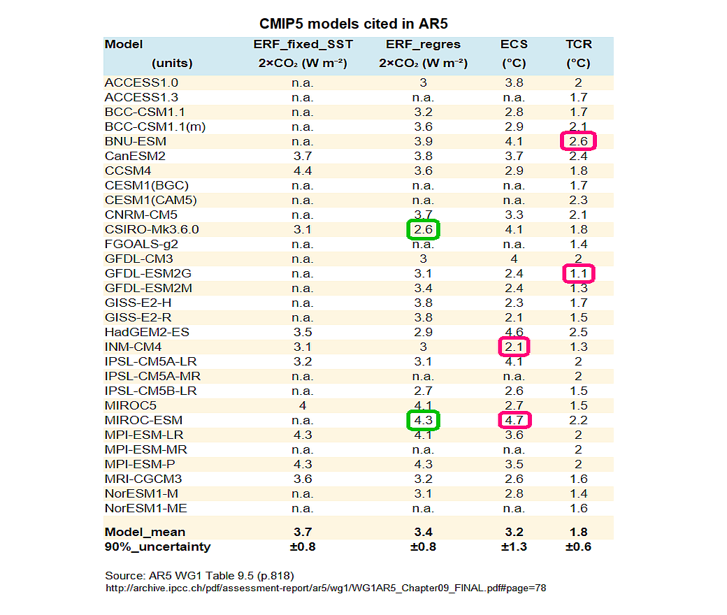
Proof that the climate modelers don’t understand what they’re modeling comes from their disagreement about basic climate parameters, like RF, TCR & ECS. If the “science were settled” GCMs wouldn’t vary drastically in their baked-in assumptions about basic climate parameters.
https://sealevel.info/AR5_Table_9.5_p.818_sensitivity_and_ERF_assumption_variations.html
How well do you think weather models would predict weather if their predictions were so far into the future they couldn’t be tested? Obviously they would be useless. But that’s exactly the situation with GCMs.
Unfortunately, most people are very good at convincing themselves of what they want to believe, regardless of the evidence — and few people want to believe that their life’s work is useless. So, the consensus among climate modelers at NASA GISS and elsewhere is that, despite the failures of earlier models, their latest sophisticated (but untestable) computer models of the Earth’s climate make reliable predictions. I think that’s wishful thinking.
Do you remember NASA’s “sophisticated computer model of the sun’s inner dynamo”? Here’s their 2006 article about it, on the eve of Solar Cycle 24:
https://science.nasa.gov/science-news/science-at-nasa/2006/21dec_cycle24/#:~:text=a%20sophisticated%20computer%20model%20of%20the%20sun%E2%80%99s%20inner%20dynamo%20to%20produce%20a%20physics%2Dbased%20prediction
Excerpt:
Of course, most WUWT readers know that Solar Cycle 24 turned out to be the weakest in a century. Oops!
The worst “models” of all (even worse than GCMs!) are so-called “semi-empirical models,” favored by PIK’s Stefan Rahmstorf and his colleagues. “Semi-empirical models” aren’t actually models at all, because they don’t even bother to try to understand and simulate reality.
Willis Eschenbach applied the equivalent of the Rahmstorf “semi-empirical modeling” approach to temperature data, and, voilà!
“Here you go, it’s the secret of climate that we’ve searched for so long,” wrote Willis. “Only problem? …”
Willis made a great point about a common scientific pitfall. Can you guess what the “problem” is? Here’s a clue.
Numbers have to be in support of a theory
There is CO2 – average temperature theory.
The only pitfall is a very rough estimate of the effect of CO2, because of a a limited ability to differentiate between natural and manmade climate change variables. Willis’s point does not apply here.
Excellent article.
A further point is to consider that if you subtract the mean model temp output from the individual model runs the residuals are largely unstructured random noise.
This tells us that (a) the model result only depends on the input forcing information (priors) which are then effectively scaled to output temps by the model parameters and (b) therefore the models don’t actually add any information. Without the variation in the priors they would simply randomly fluctuate.
Climate_model_output_temp = inputForcings*modelScaling + randomGarbage
Excellent!
I have made computer models for a living. A computer model of an air conditioning system of an office building cannot hold a single comfortable-temperature meeting. A model of elevator usage in a skyscraper does not move a single person. Models must be verified with real-world data and rejected if they do not match. The best-practice would be, as mentioned in the article, to preserve only the best and correct the model as needed.
Given that most climate models are run using 30-minute time steps or thereabouts, it would seem that a just completed climate model run could be compared to current weather models over say a ten-day period. I would be curious how they match up.
Regional climates matter. Climate models produce results for the whole world. I rarely see any comparisons from predicted regional outcomes to actual regional outcomes. If climate models can not get the regional variation correct, aggregating to a world temperature estimate makes little sense. What climate model reproduces the cooling in the SE over the last 70 years or so? What climate model reproduces the cooling we have seen in the Antarctic over the last 40 years?
It’s a very strange world where unverified model output is being touted as actual data that demands we act to reduce CO2 emissions.
Regretably, it’s not so strange. It is the predictable outcome of leftist politicians using useful idiots to provide them with talking points to control their countries. Imaginary Calamities to be saved from, as per H.L. Mencken’s observation.
I found this article really informative. For some time I have pondered how the models operated, and had worked out some of the concept, i.e. cells, the other stuff to do with variables has given me more insight.
Even so, there are still, a few questions I have, which I hope some of you people may be able to enlighten me.
Firstly, they use timesteps to determine how a cell will affect a neighbouring cell. But surely the real system is dynamic and as such there will be a dynamic simultaneous feedback, which may have a damping effect (like amplifier circuits). Additionally, this will occur not just to the two neighbouring cells bull all the adjacent cell that have an interface with each other.
To be honest, I can’t think of how one could model such a real-time system, even with a quantum computer. Is it possible?
Since it is a 3D model, I think I perceive another issue, that of adjacent cells that do not have an interface with each other. By that, I mean that a cell is a cube, and as such it has six surfaces, which interface with other cells. I assume that, it is possible to model an energy transfer across the interface. But what about the adjacent cells, that touch via a corner point or edge? In essence, there isn’t an interface and hence no energy transfer. But in reality, energy will transfer from such cells.
Finally, when running the model, one has to choose a starting point, maybe 0,0 equator, prime meridian. But what happens if the model is run from a different starting point, would the result be the same?
The feedback mechanism at each timestep is complicated. Simple models just calculate the changes at the end of the timestep to be used at the start of the next tomestep. In other words, there is no feedback calculated during the timestep.
Sophisticated models actually determine the feedback effects on each cell and then recalculate so the end of the timestep includes the feedback effects. In other words, it’s iterative. Of course this is far more intensive. Ideally there should be more than one iteration, but this is prohibitive in computer power.
There is no flow between corners, just between the model faces. Some models have hexagonal cells, but again, the computational requirement for this is immense.
The surface are of the point of a cube has zero surface area, so there is no energy transfer. This is true of models, as well as in the real world.
For the purposes of this discussion, a line is the same as a point. They both have no actual surface area.
Imagine 4 cubes, 1, 2, 3 and 4. The cubes are arrange 2 to a row and 2 rows.
1 and 2 are on top, 3 and 4 are on the bottom. 3 is below 1 and 4 is below two.
Assume cube 1 warms up. In the next time step energy is transfered from cube 1 to cubes 2 and 3. In time step two, energy is transferred from cubes 2 and 3 to cube 4.
If you wish to point out that in the real world, energy would start transferring from cube 1 to cube 4 directly, pretty much instantly, you would be correct.
However this discrepancy is not the fault of the technique of dividing the atmosphere into cubes, but rather a problem with the size of the cubes and the length of the time steps.
In the real world, each cubes that are infinitely small, and time steps are also infinitely small.
If climate models could accurately reflect the real world, they would be able to more accurately reflect real world behavior.
For any of the climate models the IPCC cites in its reports, does the author have access to the system design documentation and the code base for any of those models?
The complete technical specification and user manual for NCAR CESM is available free on line. I slogged thru v3 (about 240 very dense pages) before writing several posts here on the Trouble with Climate models, parameterization, and such. So yes, the author had it available and everything he said is factually correct. I verified myself long ago.
Thanks. Here is a further question I would have for those in the know: Is NCAR CESM fairly representative of the other climate models in terms of its internal design philosophy and its approach to using parameterization — even if its code base may not use the same programming languages and the same internal data structures as do other mainstream climate models.
Not exactly.
At the end of a shotgun barrel, there is a slight tightening of the bore during the last 4″-8″. This works like a focusing lens which is to have a shot pattern of 30″ at a specified distance. The various chokes are cylinder, improved cylinder, modified, improved modified, full chokes, each choke level represents an additional 5 yards of distance.
Technically, there are a few chokes left out; e.g., improved improved cylinder, improved improved modified and full full chokes.
Each shotgun shell has a shot cup that holds the pellets in position. Modern shot cups incorporate the pad with the shot cup, older and black powder shells have separate pads.
The pad is to contain the burning powder preventing heat damage to the pellets, while the shot cup is to prevent the pellets rolling, bouncing or skidding down the barrel.
Shooters looking to gain the maximum distance pack the pellets in a powder to help lock the pellets in position until they exit the barrel.
The barrel length aids in several ways, mostly to give the shooter a sighting base for aiming. Longer sight radiuses allow better accuracy. In this case, accuracy is defined as the shooter targeting the target which is under motion of differing and often highly variable speeds.
The barrel also allows the load to continue accelerate for a portion of the barrel as the gases finish expanding.
You are essentially correct that once the shot pattern passes the gun specific focal distance, the pattern continues to spread.
On a historical note, during the American Civil War, many soldiers shooting smoothbore rifles kept their smoothbore rifles as they preferred shooting “buck and ball” loads.
This load consists of a rifle bullet with several shotgun buckshot pellets. Keep in mind that their bullets were 0.58″ caliber and their buckshot pellets ranged from 0.30″ to 0.33″ caliber, a deadly load on a crowded battlefield.
Of course those were rifles, not shotguns…
You learn something new every day.
So climate models aren’t as accurate as shotguns.
Excellent piece and accessible. I’d like to find out how modelers constrain their models to the physically possible when forecasting steps forward. These models would obviously generate garbage if not constrained beyond the step-by-step physical processes that are modeled.
ThinkingScientist said: “A further point is to consider that if you subtract the mean model temp output from the individual model runs the residuals are largely unstructured random noise. This tells us that (a) the model result only depends on the input forcing information (priors) which are then effectively scaled to output temps by the model parameters and (b) therefore the models don’t actually add any information. Without the variation in the priors they would simply randomly fluctuate. Climate_model_output_temp = inputForcings*modelScaling + randomGarbage”
Some months ago, Willis Eschenbach used a more detailed analysis technique to arrive at that same conclusion — i.e., that the model result only depends on the input forcing information (priors) which are then effectively scaled to output temps by the model parameters — and therefore the models don’t actually add any information.
The true purpose of the climate models is to add a veneer of scientific credibility to output results already dictated by the choice of input forcing information (priors) and input model parameters. Their other true purpose is to obscure the scientific issues surrounding the choices being made for input forcing and for input parameters, hiding these choices behind a cloud of computational modeling smoke.
For purposes of supplying scientific information of real value to public policy decision makers, one could simply choose a range of values for the assumed rate of decadal rise or fall in GMT in the 21st Century. Let’s say, for example, a series of values between +0.10C and +0.30C per decade made in +0.05C per decade increments.
One could then, without ever using a computerized climate model, write up an analysis for each incremental value explaining what assumed forcings and what assumed physical parameters would make that outcome either more likely or less likely to occur between now and the year 2100.
That kind of presentation would emphasize the uncertainties in the assumed forcings and in the assumed parameters associated with each +0.05C per decade incremental value for the rise in GMT by the end of 21st Century. The presentation would also address the fact that the rate of increase in GMT has not been consistent from decade to decade, adding more uncertainty to the assumptions already being made concerning forcings and assumed physical parameters.
This kind of approach for influencing public policy decision makers will not convince the climate activists among them, nor will it convince climate activists generally. However, it will give those decision makers who oppose the insanity of Net Zero a more transparent and understandable scientific basis for their opposition.
You just described basically what Pat Frank showed with his analysis. The models are really nothing more than linear functions like y = mx + b where the “m” value is the sum of the parameterization factors. Thus uncertainty in the output grows with each iteration of the model.
The reason climate models will NEVER, and I mean NEVER, work is because they assume a linear relationship between CO2 and Temperature, and they place the majority of the explanatory power on CO2. Simply put, Temp = f(log(CO2)), not Temp = f(CO2). The whole reason for the temp data “adjustments” is to make temp more linear. That alone is a smoking gun. They clearly have intent in the adjustments, and the adjustments are made to promote a false narrative, not the reality of the science and true quantum mechanics of the CO2 molecule.
Adjusting the dependent variable in the manner they do creates a GIGO situation of epic proportions.
This is very easily testable. Simply go to NASA GISS and identify desert stations that are natural controls for the Urban Heat Island Effect and Water Vapor. What you will find are hundreds of locations that show no warming with the increase in CO2. Literally, hundreds of locations debunk the CO2 drives temperatures.
What needs to be done is real scientists need to start challenging climate scientists as to why there are so many locations that don’t show warming. Do the laws of physics cease to exist at those locations?
Lastly, the oceans are warming. CO2 and its only mechanism to affect climate is through 15-micron LWIR doesn’t penetrate or warm water. Once again, simply study the quantum mechanics of the CO2 molecule. CO2-driven warming is a monster lie.
If they would just carry through all the uncertainties in the measurements instead of just assuming that they all cancel, they would realize that they can’t tell what is actually happening at all. All the temperature changes are swamped by the total uncertainty. The global average temp could be going up, down, or sideways and there isn’t any way to tell for sure because its all hidden inside the uncertainty interval!
I used to build computer models for natural gas pipelines and can confirm this article is spot on. About 40 years ago I wrote a training manual for pipeline controllers that includes this statement: “The assumption that a steady-state condition can even exist in a flowing pipeline is ridiculous to begin with.” And this: “A pipeline flow analysis, even when computerized, consists largely of a series of estimates based on assumptions that somebody somewhere is going to object to anyway.” And pipeline models are MUCH simpler than climate models.
Mr. Chapman – Thank you for the description of how the models work. I knew a lot of it, maybe all, but never seen it all written in one place. I’ll be saving this description for future discussions.
Climate models as described remind me a lot of a software modeling tool we (and the Government) used when doing a rough check of the hours and costs of developing software. It ate at me that little tweaks to parameters such as coder experience, software complexity, past performance, etc., could make the product very affordable or very expensive. We never shared how we tweaked the parameters, and neither did the Government.
It’s been almost 13 years since I retired. Anyone who has worked on large software proposals to the Government shoud be able to remember the name of that tool.
It would be extremely helpful to update Figure 5 with data through 2022 if possible, or 2020 at least.
This chart is very, very powerful, but we really need to most recent data included to have full confidence.