By Christopher Monckton of Brenchley
On the UAH data, there has been no global warming at all for very nearly seven years since January 2015 of 2015. The New Pause has lengthened by three months, thanks to what may prove to be a small double-dip la Niña:

On the HadCRUT4 data, there has been no global warming for close to eight years, since March 2014. That period can be expected to lengthen once the HadCRUT data are updated – the “University” of East Anglia is slower at maintaining the data these days than it used to be.

Last month I wrote that Pat Frank’s paper of 2019 demonstrating by standard statistical methods that data uncertainties make accurate prediction of global warming impossible was perhaps the most important ever to have been published on the climate-change question in the learned journals.
This remark prompted the coven of lavishly-paid trolls who infest this and other scientifically skeptical websites to attempt to attack Pat Frank and his paper. With great patience and still greater authority, Pat – supported by some doughty WUWT regulars – slapped the whining trolls down. The discussion was among the longest threads to appear at WUWT.
It is indeed impossible for climatologists accurately to predict global warming, not only because – as Pat’s paper definitively shows – the underlying data are so very uncertain but also because climatologists err by adding the large emission-temperature feedback response to, and miscounting it as though it were part of, the actually minuscule feedback response to direct warming forced by greenhouse gases.
In 1850, in round numbers, the 287 K equilibrium global mean surface temperature comprised 255 K reference sensitivity to solar irradiance net of albedo (the emission or sunshine temperature); 8 K direct warming forced by greenhouse gases; and 24 K total feedback response.
Paper after paper in the climatological journals (see e.g. Lacis et al. 2010) makes the erroneous assumption that the 8 K reference sensitivity directly forced by preindustrial noncondensing greenhouse gases generated the entire 24 K feedback response in 1850 and that, therefore, the 1 K direct warming by doubled CO2 would engender equilibrium doubled-CO2 sensitivity (ECS) of around 4 K.
It is on that strikingly naïve miscalculation, leading to the conclusion that ECS will necessarily be large, that the current pandemic of panic about the imagined “climate emergency” is unsoundly founded.
The error is enormous. For the 255 K emission or sunshine temperature accounted for 97% of the 255 + 8 = 263 K pre-feedback warming (or reference sensitivity) in 1850. Therefore, that year, 97% of the 24 K total feedback response – i.e., 23.3 K – was feedback response to the 255 K sunshine temperature, and only 0.7 K was feedback response to the 8 K reference sensitivity forced by preindustrial noncondensing greenhouse gases.
Therefore, if the feedback regime as it stood in 1850 were to persist today (and there is good reason to suppose that it does persist, for the climate is near-perfectly thermostatic), the system-gain factor, the ratio of equilibrium to reference temperature, would not be 32 / 8 = 4, as climatology has hitherto assumed, but much closer to (255 + 32) / (255 + 8) = 1.09. One must include the 255 K sunshine temperature in the numerator and the denominator, but climatology leaves it out.
Thus, for reference doubled-CO2 sensitivity of 1.05 K, ECS would not be 4 x 1.05 = 4.2 K, as climatology imagines (Sir John Houghton of the IPCC once wrote to me to say that apportionment of the 32 K natural greenhouse effect was why large ECS was predicted), but more like 1.09 x 1.05 = 1.1 K.
However, if there were an increase of just 1% (from 1.09 to 1.1) in the system-gain factor today compared with 1850, which is possible though not at all likely, ECS by climatology’s erroneous method would still be 4.2 K, but by the corrected method that 1% increase would imply a 300% increase in ECS from 1.1 K to 1.1 (263 + 1.05) – 287 = 4.5 K.

And that is why it is quite impossible to predict global warming accurately, whether with or without a billion-dollar computer model. Since a 1% increase in the system-gain factor would lead to a 300% increase in ECS from 1.1 K to 4.5 K, and since not one of the dozens of feedback responses in the climate can be directly measured or reliably estimated to any useful degree of precision (and certainly not within 1%), the derivation of climate sensitivity is – just as Pat Frank’s paper says it is – pure guesswork.
And that is why these long Pauses in global temperature have become ever more important. They give us a far better indication of the true likely rate of global warming than any of the costly but ineffectual and inaccurate predictions made by climatologists. And they show that global warming is far smaller and slower than had originally been predicted.
As Dr Benny Peiser of the splendid Global Warming Policy Foundation has said in his recent lecture to the Climate Intelligence Group (available on YouTube), there is a growing disconnect between the shrieking extremism of the climate Communists, on the one hand, and the growing caution of populations such as the Swiss, on the other, who have voted down a proposal to cripple the national economy and Save The Planet on the sensible and scientifically-justifiable ground that the cost will exceed any legitimately-conceivable benefit.
By now, most voters have seen for themselves that The Planet, far from being at risk from warmer weather worldwide, is benefiting therefrom. There is no need to do anything at all about global warming except to enjoy it.
Now that it is clear beyond any scintilla of doubt that official predictions of global warming are even less reliable than consulting palms, tea-leaves, tarot cards, witch-doctors, shamans, computers, national academies of sciences, schoolchildren or animal entrails, the case for continuing to close down major Western industries one by one, transferring their jobs and profits to Communist-run Russia and China, vanishes away.
The global warming scare is over. Will someone tell the lackwit scientific illiterates who currently govern the once-free West, against which the embittered enemies of democracy and liberty have selectively, malevolently and profitably targeted the climate fraud?
”There is no need to do anything at all about global warming except to enjoy it.”
And indeed I would were it to appear…
Thank you Lord Monckton.
Yep. I was hoping for a nice warm retirement. Maybe I’ll buy new skis instead.
In my area, most of the forecasters said that the high temperature record for the date set in 1885 would be challenged. In actuality, yesterday’s high fell short of the record by 3F.
Nothing to see here, and the warm front is being replaced by a cold front, so enjoying the warmth was nice while it lasted.
Yes, enjoy the heat dome and record 40C plus temps, enjoy the 1 in 1,000 year deluges sweeping away homes and drowning the subways and cutting off your major cities, enjoy the 100 mph winds cutting off your electricity for days.
Do you imagine the examples of weather events you have highlighted, are something unique to the 21st century then, griff?
Yea, like a 1 in 100 year flood now happens every 3 months? griff depends on fellow trolls not bothering to fact-check his manifesto.
There are likely over 7 billion once in a lifetime events happening every single day.
you and griffter lack a basic understanding of statistics…
a 1 in 100 year flood in a given location occurs roughly once every 100 years
a 1 in 100 year flood across 10,000’s of different locations across the earth may very well occur once ever few months
Menace, there is nothing in weather or statististics that says you cant have three or more 100yr floods, droughts, etc within a year at one location. You may or may not thereafter see another for several hundred years. Your understanding of statistics (and weather) is that of the the innumerate majority.
Ron Long is a geologist and you can be sure he understands both stats and weather along with a heck of a lot more.
That was my understanding as well, Gary. Most people just don’t get statistics … statistically speaking, of course.
very good!
I suspect very few rivers are so well studied that it’s precisely known what the “once per century” flood might look like. But, a study of the flood plain should suffice for guidance as to what land should not be developed and if so, what sort of measures can be taken to minimize the risk. Hardly ever done of course. Instead, often wetlands in floodplains are filled in and levies are built pushing the flood downstream. Seems like more of an engineering problem, not one of man caused climate catastrophe – unless you consider bad engineering to be man caused.
@menace…. a 100 year flood has a 1% chance of occurring each and every year. It is possible to have more than one 100 year flood in a given year. Read up on recurrence intervals in any good fluvial hydraulics text book
Exactly ! As another example , proton decay. If it does decay via a positron, the proton’s half-life is constrained to be at least 1.67×1034 years , many orders of magnitude longer than the current age of the Universe . But that doesn’t stop science from spending millions of dollars on equipment and installations looking for a decay if they look at enough protons at once
Just no.
Your understanding of statistics is on par with Griff.
At the same location you can have several 1 in 100 floods in the same decade, even the same year.
Or also a 1% chance happening every year.
I suspect the idiots think- if there is a 1 in 100 year flood SOMEWHERE on the planet most years, then that proves there is a problem. After all, such a flood should only happen once per century on the entire planet. Yes, that sounds dumb but all the climatistas that I personally know think at that level.
Rod, Griff is a rabble rouser and not interested in a careful and critical evaluation of various views on climate. He needs to be totally ignored – not even given a down arrow. There are plenty of other contributors that make thoughtful contributions on this site.
Absolutely correct, the more people respond the more he will put forward his stupid observations. Can I suggest that no one responds to him at all in the future as I belief he writes his endlessly ridiculous comments merely to evoke a response rather than intellectual argument. Let us all ignore him from now on and hope that will make him go away.
Actually, it is useful that nitwits like Griff comment here: for they are a standing advertisement for the ultimate futility of climate Communism.
Christopher,
Well said. And thank you so very much for all your tireless work.
I am confident that eventually sanity will return to the world and science. But sadly I probably won’t live to see it.
Let’s hope that at least we’ve reached peak insanity. Ironically, the one thing that may help to reverse the madness is a sustained period of cooling. It’s ironical because sceptics are familiar with the history of climate – unlike clowns such as Biden and Johnson – and they understand how devestating a significant cooling would be.
So, yes, let’s enjoy this mild warming while it lasts.
Chris
You’re right once again. It’s always useful to learn what’s on the minds of your enemies, regardless how limited they may be, because, in the words of C.S. Lewis, “… those who torment us for our own good will torment us without end for they do so with the approval of their own conscience.”
I’m mindful of once well respected scientists, like Stephen Schneider who cast away professional integrity for “The Cause”.
He claimed to be in a moral dilemma where in fact there is none. He said … “we have to offer up scary scenarios, make simplified, dramatic statements, and make little mention of any doubts we might have.” committing the sin of omission and the fallacy of false dichotomy. All he ever needed to do was to follow his own words … “as scientists we are ethically bound to the scientific method, in effect promising to tell the truth, the whole truth, and nothing but”.
Once again I thank you for your integrity and hard work. If we cannot trust those who have the knowledge, were does that leave us?
Are you here just for everyone else’s entertainment? It certainly seems that way.
Griffie-poo, pray tell us when, if ever, these weather disasters did NOT occur. You can’t, of course.
You do know that the annual global death toll due to weather has been declining since the beginning of the 20th Century?
Does this also mean Winter temps in England not falling below 10C; keeping at 12 to 15C say .This will be important when we can no longer heat our homes with gas central heating.
griff, you do know you’re going to die?
Probably sooner rather than later, you’re that wound-up.
That fact is used to create fear to manipulate us, and life in many ways is a struggle to come to terms with our mortality.
I gave up on mortality around Freshman year in high school. I’d done a bit of reading I came to the conclusion just to ignore it. I believe in God because I can’t see any other way to think about the Universe. There’s really nothing t be gained by thinking to much about mortality.
It’s the truly egalitarian life.
Easy, griff, you are pointing to the alternative:
Good luck with your
climateway of life changes!…All these weatherevents during the warming pause, so it’s not related to warming, but to natural variability you just have discovered.
I see griff is still trying to convince people that prior to CO2 there was no such thing as bad weather.
Prior to Adam and Eve eating the Forbidden Fruit, the weather was constant and always like a nice day in Tahiti, and there was only enough CO2 in the air to keep the existing plants in the Garden of Eden alive. It has all been down hill since then! Even the snake has to live in the grass. Alas, we are doomed! [Imaginative sarcasm primarily for the benefit of ‘griffy.’]
…. and the idiot lives in England too.
I got out on parole after 23 years. I’m thinking of moving to Costa Rica to stay warm. This Bay Area sh!t just ain’t cutting it.
Derp
Please show your math.
Ditto
Maybe this will help:
Which means that in the approximately 20 thousand years that modern, H. sapiens have lived in Europe, there have been at least 20 such deluges. Nothing new! And, inasmuch as most cultures have legends of greater floods, we might well be in store for similar. But, it is to be expected, not the result of slight warming.
Winds were more frequent and much more ferocious at the end of the last glaciation because of the cold ice to the north and the warming bare soil exposed by the retreat of the glaciers.
You seem to be doing your hand-waving fan dance based on what you have experienced during your short life, rather than from the viewpoint of a geologist accustomed to envisioning millions and tens of millions of years. It is no wonder that you think that the sky is falling.
I know many posters know this but the pillock, Griff, is laughing at the people who take the trouble to put him/her/it right on CC etc.
You must understand, this idiot’s Mother has to lean his bed sheets against the wall to crack ’em in order to fold ’em for the wash. He’s also a waste of blog space. Please ignore him – even if you enjoy the sport.
It’s NOT about griffter, every regular here knows he’s been schooled time and time again about his baseless claims yet he persists. It’s about anyone who might be new here so they know that griffter is a despicable liar who parrots discredited BS.
About 8000 years ago, a group of several hundred people in the Himalayas were killed in a hailstorm, leaving them with tennis ball sized holes in their skulls. Weather extremes have always happened from time to time. No evidence they’re increasing now.
Hadn’t heard about that one. got a search to go to?
https://www.indiatoday.in/india/north/story/uttarakhand-roopkund-skeleton-lake-mystery-solved-bones-9th-century-tribesmen-died-of-hail-storms-165083-2013-05-31
You really need to stop posting your lack of knowledge… Take some time off, and dedicate yourself to getting a real education!
In contemporary England? Surely you jest. England stopped doing education several decades ago.
The stench of desperation in these words!
Sorry old boy, your threatened climate “attacks” have all happened now and then for over 3000 years. There were several pueblo cultures in the current Airzona/New Mexico and they lived there for centuries and prospered to the degree possible until a super drought around 1000CE and Inca invaders broke the whole area apart and died out..
Those droughts and other climate effects have returned many times over the years.
The last one was more or less in the 1930’s, further north and east. 100mph winds occur regularly, particularly in the mountainous states.
There is no need to look for “human caused” climate change. The natural changes seem to be plenty powerful and it is difficult to find any “climate changes”.
Keep in mind, the UN set up the United Nations Environment Program SPECIFICALLY to evaluate “HUMAN-CAUSED” environmental changes. No science need apply. Apparently, despite all the history, only humans can change the climate. Forget the Sun, currently in a major low point causing many effects on earth, earthquakes, fickle winds(mostly caused by the sun) and waaay more.
all of this shit has happened many times before down thru all written history.
It is nothing new, nothing catastrophic, & it sure isn’t unprecedented. No need to tell you to do some research because you won’t & besides you already know
that all you are doing is spreading bullshit & lying threw your teeth like a flim flam huckster. .
Climate Communists such as Griff are not, perhaps, aware that one would expect hundreds of 1-in-1000-year events every year, because there are so many micro-climates and so many possible weather records. They are also unaware that, particularly in the extratropics, generally warmer weather is more likely than not to lead to fewer extreme-weather events overall, which is why even the grim-faced Kommissars of the Brussels tyranny-by-clerk have found that even with 5.4 K warming between now and 2080 there would be 94,000 more living Europeans by that year than if there were no global warming between now and then.
I saw that movie too.
Now THAT’s Cognitive Dissonance if ever I saw it.
Exactly what I keep telling myself HotScot. Griff needs to take a course in human psychology to understand what is going on in his head.
I’d bet he’s getting a $1 per reply he gets, or some such. He doesn’t even make usable claims.
Global cooling trend intact since February 2016.
It’s a pleasure! On balance, one would expect global warming to continue, but these long Pauses are a visually simple demonstration that the rate of warming is a great deal less than had originally been predicted.
There has been no warming but, the science, man. The science. The science of consensus says that we’ve only got a few years left on the clock before earth becomes inhabitable. Doctor of Earthican Science, Joe Biden says we have only eight years left to act before doomsday. DOOMSDAY!
Teh siense, you meant?
Isn’t it interesting that the ones least able to fully understand ‘Science’ are the ones proclaiming it the loudest.
Yes, that is always the way. Ignorance is always demonstrated by those that lack training or rational thought.
On close inspection, Tom, it is not the science they are proclaiming. The science is untenable. So, they proclaim their virtuousness, and your/mine ignorance of the necessity to not question the science, in order to save the world from mankind’s industrial nature.
Literally! I mean it. Not figuratively. You know the thing.
More Goreball warning, as the Earth recovers from the devastating LIA. Record food crops from the delicious extra CO2.
Viscount Monckton,
Thanks for your article which I enjoyed.
Trolls make-use of minor and debateable points as distractions so I write to suggest a minor amendment to your article. Please note that this is a genuine attempt to be helpful and is not merely nit-picking because, in addition to preempting troll comments, my suggested minor amendment emphasises the importance of natural climate variability which is the purpose of your study of the ‘new pause’.
You say,
I write to suggest it would be more correct to say,
‘Therefore, if the feedback regime as it stood in 1850 were to persist today (and there is good reason to suppose that it does persist, for the climate is probably near-perfectly thermostatic), …’
This is because spatial redistribution of heat across the Earth’s surface (e.g. as a result of variation to ocean currents) can alter the global average temperature (GAT). The change to GAT occurs because radiative heat loss is proportional to the fourth power of the temperature of an emitting surface and temperature varies e.g. with latitude. So, GAT changes to maintain radiative balance when heat is transferred from a hot region to a colder region. Calculations independently conducted by several people (including me and more notably Richard Lindzen) indicate the effect is such that spatial redistribution of heat across the Earth’s surface may have been responsible for the entire change of GAT thought to have happened since before the industrial revolution.
Richard
You make a fine comment to go with CM’s article. Your assertion is one reason why using averages for the GAT makes no sense. An average only makes sense if the actual radiation occurs in that fashion. Otherwise, part of the earth (the equator) receives a predominate amount of the radiation and it reduces away from that point. Since temp is bases on an exponent of 4, the temps will also vary based on this factor. Simple averages and “linear” regression, homogenization, etc. simply can not follow the temps properly.
Richard Courtney asks me to add a second qualifier, “probably”, to the first, “near”, in the sentence “The climate is near-perfectly thermostatic”. However, Jouzel et al. (2007), reconstructing the past 810,000 years’ temperatures in Greenland by cryostratigraphy, concluded that in all that time (after allowing for polar amplification) global temperatures varied by little more than 3 K either side of the period mean. The climate is, therefore, near-perfectly thermostatic. Compensating influences such as Eschenbach variability in tropical afternoon convection keep the temperature within quite narrow bounds.
And owing to the fact that the vast majority, 99.9% of the earth’s surface is constantly exposed to deep space at near absolute zero and the Sun takes up such a small heat source in area it is remarkable that it does keep such a good control of temperature. I put that control largely down to clouds especially at night time in winter .
Of the numerous thermostatic processes in climate, the vast heat capacity of the ocean is probably the most influential.
Most voters believe that climate change is real and dangerous because they are force fed a constant diet of media alarmism, supported by dim politicians and green activists. It is so uncool [no pun intended] to be a climate heretic when the religious orthodoxy promotes ideological purity and punishes rational thinking.
Most people are uncomfortable living outside the orthodoxy especially when one is exposed to a constant barrage of dogma reinforcing it every minute. The media, now acting as the public relations branch of “progressive” governments, tailor their reporting to suit.
“…the “University” of East Anglia is slower at maintaining the data these days than it used to be…”
Hey, they’ve been really busy. Those “adjustments” don’t do themselves, you know.
uEA is now redundant. Stock markets do the predictions – FTse100 is currently running at 2,7C and needs to divest itself of commodities, oil and gas to reach the magic 1.5C. I don’t know where they imagine the materials will come from for their electric cars, heat pumps, wind farms, mobile phones, double glazing etc. No doubt China will step in to save the day just before we run into the buffers.
Wind turbines are self replicating organisms dontchaknow. That’s why the electricity they produce is so cheap.
It is only “cheap” if you live in never ending wind land , otherwise you have to keep a gas fired power plant idling in the background , MW for MW .
Truth be known, UEA is now only half-fast compared to what they used to be.
UAH is a multiply adjusted proxy measurement of the Troposphere, which doesn’t even agree with similar proxy Tropospheric measurements (why do these pages never mention RSS these days?).
I think we have to take it as at least an outlier and quite probably not representative of what’s happening.
Predictable attempt to discredit the most reputable and accurate measuring system we have.
The irony is that if UAH cannot be relied on then nor can any other system of measurement.
Would be interested to know the trend from the old pause at its maximum including the new pause.
I imagine it would be Roy’s 0.14 trend but. It might be lower.
So 1997? to 2021?
Depends on when exactly you think the old pause started. Cherry picking the lowest and longest trend prior to 1998, the trend from April 1997 is 1.1°C / decade.
Starting just after the El Niño the trend from November 1998 is 1.6°C / decade.
Did you enjoy Antarctica’s second coldest winter on record? I know I did.
How was the UK’s 3rd warmest autumn for you, fret? Did you manage to find your usual cloud?
What will you make of the situation if next year it is the 4th warmest Autumn? Or even if it is tied with this year? Do you really believe that the ranking has any significance when depending on hundredths of a degree to discriminate?
Did you not learn anything, ToeFungalNail? When the difference in temperature is less than the measurement error any ranking of the warmest month, year, or season is bogus. Why do you persist in (fecklessly) trying to mislead?
-51 oC central Greenland last week , coldest I have ever seen that !
I assume you mean 0.11 and 0.16 C/decade
the old pause started prior to 1997 El Nino spike, there was never pause starting from post-spike… indeed it is that large spike that made the long statistical “pause” possible
Yes, sorry. Good catch. I was thinking of the per century values.
I’m not sure if anyone sees the irony of claiming that a pause only exists prior to a temperature spike and vanishes if you start after the spike.
Bellman,
Your comment is lame and demonstrates you do not understand the calculation conducted by Viscount Monckton. I explain as follows.
(a)
The “start” of the assessed pause is now
and
(b) the length of the pause is the time back from now until a trend is observed to exist at 90% confidence within the assesedd time series of global average temperature (GAT).
The resulting “pause” is the length of time before now when there was no discernible trend according to the assessed time series of GAT.
I see no “irony” in the “pause” although its name could be challenged. But I do see much gall in your comment which attempts to criticise the calculation while displaying your ignorance of the calculation, its meaning, and its indication.
Richard
I’ve already answered this a couple of times, but no, Monckton’s pause is not based on confidence intervals, nor have I ever seen him claim that it starts at the end. Here’s Monckton’s definition
If you think you understand how the pause is calculated better than me, feel free to calculate when the pause should have started or ended this month and share your results, along with the workings.
For my part, I just have a function in R that calculates the trend from each start date to the current date, and then I just look back to see the earliest negative value. I could get the earliest date programmatically, but it’s useful to have a list of all possible trends, just to see how much difference a small change in the start date can make.
Bellman,
I object to you blaming me for your inability to read.
I said,
(a)
The “start” of the assessed pause is now
and
(b) the length of the pause is the time back from now until a trend is observed to exist at 90% confidence within the assessed time series of global average temperature (GAT).
You quote Viscount Monckton as having said,
As usual, the Pause is defined as the longest period, up to the most recent month for which data are available, during which the linear-regression trend on the monthly global mean lower-troposphere temperature anomalies shows no increase.
The only difference between those two explanations is that
I state the confidence (90%) that is accepted as showing no change (or ” no increase”) normally applied in ‘climate so-called science’
but
the noble Lord assumes an interested reader would know that.
I assume your claim that you cannot read is sophistry intended to evade the need for you to apologise for having posted nonsense (i.e. you don’t want to say sorry for having attempted ‘bull sh** baffles brains’)
Richard
“The only difference between those two explanations is that
I state the confidence (90%) that is accepted as showing no change”
And that’s where your method is different from Lord Monckton’s. And no amount of personal insults will convince me you are right and I’m wrong. I said before, if you want to convince me about your 90% confidence interval approach, actually do the work, show me how that will make January 2015 the start date this month.
Here’s some of my workings, each value represents the trend in degrees per century starting at each month.
The pause starts on January 2015, because that is the earliest month with a zero trend, actually -0.03.
If you wanted to go back as far as possible to find a trend that was significant at the 90% level the pause would be much longer.
“(b) the length of the pause is the time back from now until a trend is observed to exist at 90% confidence within the assessed time series of global average temperature (GAT).2”
Please provide a link to where Monckton says that he uses 90% confidence limits.
He doesn’t.
And, what’s more he doesn’t have to, as denizens don’t require it and he ignores all critics with bluster and/or ad hom.
In short he has blown his fuse and this place is the only one he can get traction for his treasured snake-oil-isms.
Forgot:
(the real driving motivation for his activities, so apparent in his spittle-filled language) …..
Accusing all critics of being communists or paid trolls.
Quite, quite pathetic.
And this is the type of science advocate (let’s not forget with diplomas in journalism and the Classics) who you support to keep your distorted view if the world and its climate scientists away from reality.
Paid climate Communists such as Bellman will make up any statistic to support the Party Line and damage the hated free West. The UAH global mean lower-troposphere temperature trend from April 1997 to November 2021 was 0.1 C/decade, a rate of warming that is harmless, net-beneficial and consistent with correction of climatology’s elementary control-theoretic error that led to this ridiculous scare in the first place.
Ad hominems aside I’d be grateful if you could point out where you think my statistics are wrong or “made up”.
Given that there is currently a lively discussion going on between me and Richard S Courtney about how you define the pause this would be a perfect opportunity to shed some light on the subject – given you are the only one who knows for sure. I say it is based on the longest period with a non-positive trend, whilst Courtney says it is the furthest you can go back until you see a significant trend.
It would be really easy to say Courtney is correct and here’s why, or no sorry Courtney, much as it pains me to say it, the “paid climate communist” is right on this one.
The furtively pseudonymous “Bellman” asks me to say where what it optimistically calls its “statistics” are wrong. It stated, falsely, that the world was warming at 1.1 C/decade, when the true value for the relevant period was 0.1 C/decade.
It was an honest mistake, for which I apologized several days ago when it was pointed out
https://wattsupwiththat.com/2021/12/02/the-new-pause-lengthens-by-a-hefty-three-months/#comment-3402617
Maybe, if you had just asked if it was correct, instead of making snide innuendos, I could have set the record straight to you as well. Unfortunately the comment system here doesn’t allow you to make corrections after a short time, and any comment I add will appear far below the original mistake.
For the record, here’s what the comment should have said
As an aside, I like the fact that Monckton is accusing me of making up statistics to “support the Party Line and damage the hated free West”, when I’m actually using the statistics to support his start date for the pause.
Unclear what you had in mind when you wrote the phrase “the old pause at its maximum” here …
… I’ll take it as “(the start of) the longest zero-trend period in UAH (V6)”, which is May 1997 to December 2015.
I haven’t updated my spreadsheet with the UAH value for November yet (I’ll get right on that, promise !), but the values for “May 1997 to latest available value” are included in the “quick and dirty” graph I came up with below.
Notes
1) UAH can indeed be considered as “an outlier” (along with HadCRUT4).
2) UAH trend since (May) 1997 is between 1.1 and 1.2 (°C per century), so your 1.4 “guesstimate” wasn’t that far off.
HadCRUT4 trend is approximately 1.45.
The other “surface (GMST) + satellite (LT)” dataset trends are all in the range 1.7 to 2.15.
3) This graph counts as “interesting”, to me at least, but people shouldn’t try to “conclude” anything serious from it !
It is important to remember that the UAH lower troposphere temperature is a complex convolution of the 0-10km temperature profile which decreases exponentially with altitude; it is not the air temperature at the surface.
And the GHE occurs at altitude in the Troposphere.
Ergo the IPCC tropospheric hotspot.
Stephen, actually, GISS and UAH used to be very closely in agreement until Karl (from which I coined the term “Karlization of temperatures” ‘adjusted’ us out of the Dreaded Pause^тм in 2015 on the eve if his retirement. Mearns, who does GISS’s satellite Ts then responded with his complementary adjustments. It bears mentioning that Roy Spencer invented the method and was commended for it by NASA at the time.
Karl added 0.12 C to the ARGO data to “be consistent with the [lousy] ship engine intake data.” This adds an independent warming trend over time as more and more ARGO floats come into the datasets, replacing the use of engine intakes in ongoing data collection.
Karl also used Night Marine Air Temperatures (NMAT) to adjust SSTs. Subsequent collected data have shown NMAT diverging from SST significantly. Somebody should readdress his “work.”
UAH is an honest broker that both sides can agree upon.
Yep but it is not a measurement of the earths surface, so useful but not the full picture.
Cooling earth is to see 2-3 month later in the lower troposphere.
Exactly Simon, we need to include the temps inside a volcano to get the full picture.
You might think that but I am for going with all the recognised data sets to get the full picture.
Just like Russia colluuuusion 😉
Duh… the one trick pony is now a no trick ass.
Are you calling yourself an ass?
Russia colluuuusion indeed. Along with your Xenophobia..that one always cracks me up.
No quarrel with that, but realize the limitations of each dataset. The “Karlized” set should not be used for scientific analyses. Also, RSS needs to explain its refusal to dump obviously bad data. Additionally, their method for estimating drift is model based as opposed to UHA’s empirical method.
Why would you measure the earths surface? Asphalt can get up to enormous temperatures not representative of the air on a sunny day. The entire point of measuring the lower troposphere is that it won’t have UHI.
That’s how they originally sold the satellites to Congress.
“Why would you measure the earths surface? “
Umm because we live here, or at least I do.
Ummm, no. You live in the lower part of the atmosphere, not in the surface! The surface is the ocean and land, e.g.. the “solid” part of the planet. The atmosphere is the gaseous part of the planet. The atmosphere is an insulator and it has a gradient from the boundary with the surface and toward space. The surface has a gradient in two directions downward and upward into the atmosphere.
Do you live in a rural location or in a city? It makes a big difference in measured temperatures.
Simon: Happily for you, UAH does agree with the direct measurements of balloon sondes. Agreement with independent measures is, of course the highest order of validation. The good fellow who invented it, Dr. Roy Spencer received a prestigious commendation of NASA back in the days when that meant a lot.
Look I have no issue with UAH, it is just not the complete picture. It has also had a lot of problems going back so anyone who thinks it is the be all and end all is, well, wrong.
And you think any of the lower atmosphere temperature data sets don’t have problems going back? They are probably less reliable because of coverage issues and the methods used to infill.
”Look I have no issue with UAH”……”( I’m just uncomfortable with what it’s showing)”
…. and it is due to natural variability.
When solar magnetic activity is high TSI goes up and warms the land and oceans. When magnetic activity goes down there is flood in of energetic GCRs which enhances cloud formation. Clouds increase albedo which should reduce atmospheric warming, but clouds also reduce heat re-radiation back into space.
Balance between two is important factor for the atmospheric temperature status, and at specific levels of reduction of solar activity the balance is tilted towards clouds warming effect.
Hence, we find that when global temperature is above average and amount of ocean evaporation is also above average, during falling solar activity there will be mall increase in the atmospheric temperature.
http://www.vukcevic.co.uk/UAH-SSN.gif
After prolonged period of time (e.g. Grand solar minima) oceans will cool, evaporation will fall and the effect will disappear.
“UAH is an honest broker that both sides can agree upon.”
Yet ever since UAH showed a warmer month one side keeps claiming satellite data including UAH is not very reliable. See carlo, monte’s analysis
https://wattsupwiththat.com/2021/12/02/uah-global-temperature-update-for-november-2021-0-08-deg-c/#comment-3401727
according to him the monthly uncertainty in UAH is at least 1.2°C.
Bellman said: “according to him the monthly uncertainty in UAH is at least 1.2°C.”
Which is odd because both the UAH and RSS groups using wildly different techniques say the uncertainty on monthly global mean TLT temperatures is about 0.2. [1] [2]
Why do you continue to use the word “uncertainty” when you don’t understand what it means?
Comparisons of line regressions against those from radiosondes is NOT an uncertainty analysis.
I use the word uncertainty because we don’t know what the error is for each month, but we do know that the range in which the error lies is ±0.2 (2σ) according to both UAH and RSS.
Note that I have always understood “error” to be the difference between measurement and truth and “uncertainty” to be the range in which the error is likely to exist.
Which is a Fantasy Island number, demonstrating once again that you still don’t understand what uncertainty is.
I compared UAH to RATPAC. The monthly differences fell into a normal distribution with σ = 0.17. This implies the an individual uncertainty of each of 2σ = 2*√(0.17^2/2) = 0.24 C which is consistent with the Christy and Mears publications. Note that this is despite UAH having a +0.135 C/decade trend while RATPAC is +0.212 C/decade so the differences increase with time due to one or both of these datasets having a systematic time dependent bias. FWIW the RSS vs RATPAC comparison implies an uncertainty of 2σ = 0.18 C. It is lower because differences do not increase with time like what happens with UAH. The data is inconsistent with your hypothesis that the uncertainty is ±1.2 C by a significant margin.
tell us again how temps recorded in integers can be averaged to obtain 1/100th of a degree. The uncertainty up to at least 1980 was a minimum of ±0.5 degrees. It is a matter of resolution of the instruments used and averaging simply can not reduce that uncertainty.
As Carlo, Monte says, “Comparisons of line regressions against those from radiosondes is NOT an uncertainty analysis.”
Linear regression of any kind ignores cyclical phenomena from 11 year sunspots, to 60 years cycles of ocean currents, to orbital variation.
Even 30 years for “climate change” ignores the true length of time for climate to truly change. Tell what areas have become deserts in the 30 to 60 years. Have any temperate boundaries changed? Have savannahs enlarged or shrunk due to temperature? Where in the tropics has become unbearable due to temperature increases?
Uncertainty: parameter, associated with the result of a measurement, that characterizes the dispersion of the values that could reasonably be attributed to the measurand.
If the uncertainty of a monthly UAH measurement is 1.2°C, then say if the measured value is 0.1°C, you are saying it’s reasonable to say the actual anomaly for that month could be between -1.1 and +1.3. If it’s reasonable to say this, you would have to assume that at least some of the hundreds of measured values differ from the measurand by a at least one degree. If you compare this with an independent measurement, say radiosondes or surface data, there would be the occasional discrepancy of at least one degree. The fact you don;t see anything like that size of discrepancy is evidence that your uncertainty estimate is too big.
UNCERTAINTY DOES NOT MEAN RANDOM ERROR!
You still have no idea of the difference between error and uncertainty. Uncertainty is NOT a dispersion of values that could reasonably be attributed to the measurand. That is random error. Each measurement you make of that measurand has uncertainty. Each and every measurement has uncertainty. You simply can not average uncertainty away as you can with random errors. What that means is that your “true value” also has an uncertainty that you can not remove by averaging.
As to your comparison. You are discussing two measurands using different devices. You CAN NOT compare their uncertainties nor assume that measurements will range throughout the range.
Repeat this 1000 times.
“UNCERTAINTY IS WHAT YOU DON’T KNOW AND CAN NEVER KNOW!”
Why do you think standard deviations are accepted as an indicator of what uncertainty can be. Standard deviations tell you what the range of values were while measuring some measurand. One standard deviation means that 68% of the values fell into that range. It means your measured values of the SAME MEASURAND will probably fall within that range. It doesn’t define what your measurement will be, only what range it could fall in.
Your assertion is a fine example of why scientific measurements should never be stated with including an uncertainty range. Not including this information leads people into the mistaken view that measurements are exact.
“Uncertainty is NOT a dispersion of values that could reasonably be attributed to the measurand.”
That is literally how the GUM defines it
“As to your comparison. You are discussing two measurands using different devices. You CAN NOT compare their uncertainties nor assume that measurements will range throughout the range.”
I’m not saying compare their uncertainties, I’m saying having two results will give you more certainty. I’m really not sure why you wouldn’t want a second opinion if the exact measurement is so important. You know there’s an uncertainty associated with your first measurement, how can double checking the result be a bad thing?
““UNCERTAINTY IS WHAT YOU DON’T KNOW AND CAN NEVER KNOW!””
I don’t care how many times you repeat this, you are supposed to know the uncertainty. Maybe you mean you can never know the error, but as you keep saying error has nothing to do with uncertainty I’m not sure what you mean by this.
“I’m saying having two results will give you more certainty.”
Only if you are measuring the SAME THING. This will *usually* generate a group of stated values plus random error where the random errors will follow a gaussian distribution and will tend to cancel out. Please note carefully that uncertainty is made up of two factors, however. One factor is random error and the other is systemic error. Random error will cancel, e.g. reading errors, systemic error will not.
If you are measuring *different* things then the errors will most likely not cancel. When measuring the same thing the stated values and uncertainties cluster around a true value. When measuring different things, the stated values and uncertainties do not cluster around a true value. There is no true value. In this case no number of total measurements will lessen the uncertainty associated with the elements themselves or the uncertainties associated with the calculated mean.
“I don’t care how many times you repeat this, you are supposed to know the uncertainty.”
Uncertainty is not error. That is a truism. Primarily because uncertainty is made up of more than one factor. If I tell you that the uncertainty of a measurement is +/- 0.2 can you tell me how much of that uncertainty is made up of random error and how much is made up of other factors (e.g. hysteresis, drift, calibration, etc)?
If you can’t tell me what each factor contributes to the total uncertainty then you can’t say that uncertainty *is* error because it is more than that. Uncertainty is not error.
“Only if you are measuring the SAME THING.”
In this case, you are measuring the same thing.
“Random error will cancel, e.g. reading errors, systemic error will not.”
Which is why it’s a good thing you are using different instruments.
“If you are measuring *different* things then the errors will most likely not cancel.”
Why not.
“When measuring different things, the stated values and uncertainties do not cluster around a true value”
Of course they do. The true value is the mean, each stated value is a distance from the mean.
“Uncertainty is not error.”
You don’t know the error, you do know the uncertainty.
“If I tell you that the uncertainty of a measurement is +/- 0.2 can you tell me how much of that uncertainty is made up of random error”
When you are stating uncertainty you should explain how it was established.
Also note, that systematic error’s are at least as much of a problem if you are measuring the same thing, than if you are measuring different things.
Why are you so desperate to make uncertainty as small as possible?
I’d have thought it was always going to be a good idea to be as certain as possible. Why would you want to be less certain?
How in the world did you jump to this idea? I never said or implied this. Instead I’ve been trying to show you how temperature uncertainties used in climastrology are absurdly small, or just ignored completely.
I was being flippant with your question, “Why are you so desperate to make uncertainty as small as possible?”
And yet the fact remains, that temperature uncertainties used in climastrology are absurdly small, or just ignored completely. Subtracting baselines does NOT remove uncertainty.
But it isn’t a fact, just your assertion. You say they are small because you can’t believe they could be so small, and in contrast give what to me seem absurdly large uncertainties.
Then you again make statements like “Subtracting baselines does NOT remove uncertainty”, as if merely you saying it makes it so.
I’m finished trying to educate you lot, enjoy life on Mars.
“Also note, that systematic error’s are at least as much of a problem if you are measuring the same thing, than if you are measuring different things”
So what? In one case you will still get clustering around a “true value” helping to limit random error impacts. In the other you won’t.
The so what, is it’s a good idea to measure something with different instruments using different eyes.
Look at the word you used — error. ERROR IS NOT UNCERTAINTY!
I can use a laser to get 10^-8 precision. Yet the uncertainty still lies with at least +/-10^-9. A systematic ERROR will still give good precision but it will not be ACCURATE!
Sorry if I’ve offended you again, but it was the Other Gorman who used the dreaded word.
“Uncertainty is not error. That is a truism. Primarily because uncertainty is made up of more than one factor. If I tell you that the uncertainty of a measurement is +/- 0.2 can you tell me how much of that uncertainty is made up of random error and how much is made up of other factors (e.g. hysteresis, drift, calibration, etc)?”
Rather than endlessly shout UNCERTAINTY IS NOT ERROR to a disinterested universe, it would be a lot more useful if you explain what you think uncertainty is. I’ve given you the GUM definition and you rejected that. I’ve tried to establish without success, is you definition has any realistic use. All you seem to want is for it to be a word that can mean anything you want. You can tell me the uncertainty in global temperatures is 1000°C, but any attempt to establish if that means you realistically think gloabal temperatures could be as much as 1000°C is just met with UNCERTAINTY IS NOT ERROR.
Sorry, that’s just not so. If uncertainty was error then the GUM definition wouldn’t state that after error is analyzed there still remains an uncertainty about the stated result.
It is *you* that keeps on rejecting that.
although error and error analysis have long been a part of the practice of measurement science or metrology.
It is now widely recognized that, when all of the known or suspected components of error have been
evaluated and the appropriate corrections have been applied, there still remains an uncertainty about the
correctness of the stated result, that is, a doubt about how well the result of the measurement represents the
value of the quantity being measured.”
This is the GUM definition. Please note carefully that it specifically states that uncertainty is not error. All the suspected components of error can be corrected or allowed for and you *still* will have uncertainty in the result of the measurement.
All this means is that once the uncertainty in your result exceeds physical limits that you need to re-evaluate your model. Something is wrong with it! In fact, if you are trying to model the global temperature to determine a projected anomaly 100 years in the future, and the uncertainty in your projection exceeds the value of the current temperature then you need to stop and start over again. For that means your model is telling you something you can’t measure! Anyone can stand on the street corner with a sign saying the world will end tomorrow. Just how much uncertainty is there in such a claim? If the sign says it will be 1C hotter tomorrow just how much uncertainty is there in such a claim?
And what the climatologists fail to recognize is that the correction factors themselves also have uncertainty that must be accounted for.
Hadn’t thought of that! Just keep going down the rabbit hole!
“Sorry, that’s just not so.”
I was talking to Jim, reminding him he rejected the error free definition of measurement uncertainty, as well as the definitions based on error.
“All this means is that once the uncertainty in your result exceeds physical limits that you need to re-evaluate your model.”
Really? You can’t accept the possibility that what it tells you is your uncertainty calculations are wrong?
“I can use a laser to get 10^-8 precision. Yet the uncertainty still lies with at least +/-10^-9.”
You keep confusing precision with resolution. If that’s not clear let me say RESOLUTION IS NOT PRECISION.
“A systematic ERROR will still give good precision but it will not be ACCURATE!”
Yes, that’s why I’m saying it’s useful to measure something twice with different instruments, even if their resolution is too low to detect random errors.
Oh yeah, you’re the world’s expert on all things metrology, everyone needs to listen up.
How many of those dozens of links that Jim has provided to you on a silver platter have you studied? Any?
No, you are just like Nitpick Nick Stokes, who picks at any little thing to attack anyone who threatens the global warming party line.
Go read his web site, he’ll tell you what you want to hear.
“Oh yeah, you’re the world’s expert on all things metrology, everyone needs to listen up.”
I am absolutely not an expert on anything – especially metrology. If I appear to be it’s because I’m standing on the shoulders of midgets.
“How many of those dozens of links that Jim has provided to you on a silver platter have you studied? Any?”
Enough to know that any he posts directly contradict his argument. Honestly the difference between SD and SEM is well documents, well known and Jim is just wrong, weirdly wrong, about them.
“No, you are just like Nitpick Nick Stokes, who picks at any little thing to attack anyone who threatens the global warming party line.”
I’m flattered that you compare me with Stokes.
The truth finally emerges from behind the greasy green smokescreen…
So Señor Experto, do tell why machine shops all don’t have a battalion of people in the backroom armed with micrometers to recheck each and every measurement 100-fold so that nirvana can be reached through averaging?
Finally, a sensible question, though asked in a stupid way.
Why don;t machine shops all make hundreds of multiple readings to increase the precision of their measurements? I think Bevington has a section on this that sums to up well. But the two obvious reasons are
1) it isn’t very efficient. Uncertainty decreases with the square root of the number of samples, s the more you do the less of a help it is. Take four measurements and you might have halved the uncertainty, but to get to a tenth the uncertainty, and hence that all important extra digit would require 100 measurements, and to get another digit is going to require 10000 measurements. I can’t speak for how machine shops are organized, but I can’t imagine it’s worth employing that many people just to reduce uncertainty by a hundredth. If you need that extra precision it’s probably better to invest in better measuring devices.
2) as I keep having to remind you, the reduction in uncertainty is a theoretical result. Taking a million measurements won’t necessarily give you a result that is 1000 times better. The high precision is likely to be swamped out by any other small inaccuracies.
Efficiency isn’t the point, you are running around the bush to try and and not answer the question. The question is whether it can be done with more measurements.
And he ran away from the inconvenient little fact is that no machine shop has a backroom filled with any people who do nothing repeat others’ measurements, not 100, not 20, not 5, not 1.
“Efficiency isn’t the point”
Really, wasn’t the question
“do tell why machine shops all don’t have a battalion of people in the backroom armed with micrometers to recheck each and every measurement 100-fold so that nirvana can be reached through averaging?”
I’m really not convinced by all these silly hypothetical questions, all of which seem to be distracting from the central question, which is does in general uncertainty increase or decrease with sample size.
Honestly the difference between SD and SEM is well documents, well known and Jim is just wong, weirdly wrong, about them.
If I am so wrong why don’t you refute the references I have made and the inferences I have taken from them. Here is the first one to refute.
SEM = SD / √N, where:
SEM is the standard deviation of the sample means distribution
SD is the standard deviation of the population being samples
N is the sample size taken from the population
What this means is you need to decide what you have in a temperature database. Do you have a group of samples or do you have a population of temperatures.
This is a simple decision to make, which is it?
I don’t need to refute the references because they agree with me.
“SEM = SD / √N, where:
SEM is the standard deviation of the sample means distribution
SD is the standard deviation of the population being samples
N is the sample size taken from the population”
See, that’s what I’m saying and not what you are saying. You take the standard deviation of the sample, which is an estimate of the SD of the population, and then think that is the standard error of the mean. Then you multiply the sample standard deviation by √N in the mistaken believe that this will give you SD.
In reality you divide the standard standard deviation by √N to get the SEM. This is on the assumption that the sample standard deviation is an estimate of SD.
Here’s a little thought experiment to see why this doesn’t work. You took a sample of size 5, took it’s standard deviation and multiplied by √5 to get a population standard deviation more than twice as big as the sample standard deviation. But what if you’d taken a sample of size 100, or 1000 or whatever. Using your logic you would multiply the sample deviation by √100 or √1000. This would make the population deviation larger the bigger your sample size. But the population standard deviation is fixed. It shouldn’t change depending on what size sample you take. Do you see the problem?
“What this means is you need to decide what you have in a temperature database. Do you have a group of samples or do you have a population of temperatures.
This is a simple decision to make, which is it?”
Of course you don;t have the population of temperatures. The population is all temperatures across the planet over a specific time period. It’s a continuous function and hence infinite. You are sampling the population in order to estimate what the population mean is.
They use temperatures from one location to infill temps at other locations. So what components of the population don’t you have? Are you saying you need a grid size of 0km,0km in order to have a true population?
Sampling only works if you have a homogenous population to sample. Are the temps in the northern hemisphere the same as the temps in the southern hemisphere? How does this work with anomalies?
Well yes, that’s what sampling is. Taking some elements as an estimate of what the population is. Of course, as I’ve said before the global temperature is not a random sample, and you do have to do things like infilling and weighting which is why estimates of uncertainty are complicated.
This is just more jive-dancing bullsh!t, you are not sampling the same quantity. You get one chance and it is gone forever.
“In reality you divide the standard standard deviation by √N to get the SEM. This is on the assumption that the sample standard deviation is an estimate of SD.”
If you already have the SD of the population then why are you trying to calculate the SEM? The SEM is used to calculate the SD of the population! If you already have the SD of the population then the SEM is useless!
You have to know the mean to calculate the SD of the population and you have to know the size of the population to calculate the mean. That implies you know the mean exactly. it is Σx/n where x are all the data values and n is the number of data values. Thus you know the mean exactly. And if you know the mean exactly and all the data values along with the number of data values then you know the SD exactly.
The SEM *should* be zero. You can’t have a standard deviation with only one value – i.e. the mean which you have already calculated EXACTLY!
This is why you keep getting asked whether your data set is a sample of if it is a population!
“DON’T confuse me with facts, my mind is MADE UP!“
What facts? Someone makes a claim that the sample standard deviation is the standard error of the mean. Something which anyone with an elementary knowledge of statistics know to be wrong and can easily be shown to be wrong. But I’m always prepared to be proven wrong, and that someone has given me an impressive list of quotes, from various sources, except that none of the quotes says that the sample standard deviation is the same as the standard error of the mean, and most say the exact opposite.
Why do I need to read the full contents of all the supplied documents. If you are making an extraordinary claim don’t throw random quotes at me – show me something that supports your claim.
“The standard error of the sample mean depends on both the standard deviation and the sample size, by the simple relation SE = SD/√(sample size). The standard error falls as the sample size increases, as the extent of chance variation is reduce”
From:
https://www.ncbi.nlm.nih.gov/pmc/articles/PMC1255808/
“However, the meaning of SEM includes statistical inference based on the sampling distribution. SEM is the SD of the theoretical distribution of the sample means (the sampling distribution).”
From:
https://www.investopedia.com/ask/answers/042415/what-difference-between-standard-error-means-and-standard-deviation.asp
Here is an image from:
https://explorable.com/standard-error-of-the-mean
Yes all three posts are saying exactly what I’m saying. Why do you think I’m wrong?
You say in a prior post that the “sample standard deviation IS NOT the standard error of the mean. Did you read what I posted?
Let me paraphrase, the Standard Error of the (sample) Mean, i.e., the SEM, is the Standard Deviation of the sample means distribution.
Look at the image.
If (qbar) has a distribution then there must be multiple samples, each with their own (qbar). By subtracting (qbar) from each value you are in essence isolating the error component.
Lastly, this is dealing with one and only one measurand. What the GUM is trying to do here is find the interval within which the true value may lay. This is important because it acknowledges that random errors quite probably won’t be removed by doing only a few measurements. If they did, the experimental standard deviation of the mean would be zero thereby indicating that there is no error left. The distribution of (qbar) would be exactly normal.
One should keep in mind that this is only dealing with measurements and error and in no way assesses the uncertainty of each measurement.
“You say in a prior post that the “sample standard deviation IS NOT the standard error of the mean. Did you read what I posted?”
Yes based on this comment, where you multiplied the standard deviation of a set of 5 numbers by √5 to calculate the standard deviation of the population.
The sample standard deviation is not the same thing as the standard error of the mean.
“Let me paraphrase, the Standard Error of the (sample) Mean, i.e., the SEM, is the Standard Deviation of the sample means distribution.”
Correct, but standard deviation of the sample means, is not the same as the standard deviation of the sample.
“If (qbar) has a distribution then there must be multiple samples, each with their own (qbar).”
No, there do not have to be literal samples. The distribution exists an abstract idea. If you took an infinite number of samples of a fixed size there would be the required distribution, but you don’t need to physically take more than one sample to know that the distribution would exist, and you can estimate it from your one sample.
It would in any event be a pointless exercise becasue if you have a large number of separate samples, the mean of their means would be much closer to the true mean. There would be no point in working out how uncertain each sample mean was, when you’ve now got a better estimate of the mean.
This nonsense constitutes “debunking” in your world?
You *HAVE* to be trolling, right? How do you get a DISTRIBUTION without multiple data points?
Total and utter malarky! Again, with one data point how do you define a distribution, be it literal or virtual?
Multiple samples allow you to measure how good your estimate is. A single sample does not! There is no guarantee that one sample consisting of randomly chosen points will accurately represent the population. And with just one sample you have no way to judge how representative the sample mean and standard deviation is of the total population.
Look at what *YOU* said: “The sample standard deviation is not the same thing as the standard error of the mean.”
When you have only one sample you are, in essence, saying the sample standard deviation *is* the standard deviation of the sample means. You can only have one way. Choose one or the other.
“True mean”? You *still* don’t get it, do you?
“There would be no point in working out how uncertain each sample mean was, when you’ve now got a better estimate of the mean.”
And, once again, you advocate for ignoring the uncertainty of the data points. If your samples consist only of stated values and you ignore their uncertainty then you have assumed the stated values are 100% accurate.
If you data set consists of the total population, with each data point consisting of “stated value +/- uncertainty” then are you claiming that the mean of that total population has no uncertainty? That each stated value is 100% accurate? If so then why even include uncertainty with the data values?
If mean of the total population has an uncertainty propagated from the individual components then why doesn’t samples from that population have an uncertainty propagated from the individual components making up the sample? How can the population mean have an uncertainty while the sample means don’t?
“You *HAVE* to be trolling, right? How do you get a DISTRIBUTION without multiple data points?”
“Total and utter malarky! Again, with one data point how do you define a distribution, be it literal or virtual?”
So you didn’t read any of the links I gave you?
I did read your links. And I told you what the problems with them were. And you *still* haven’t answered the question. How do you get a distribution without multiple data points.?
Fine, disagree with every text book on the subject, because they don’t understand it’s impossible to work out the SEM from just one sample. Just don’t expect me to follow through your tortured logic.
“And you *still* haven’t answered the question. How do you get a distribution without multiple data points.?”
The distribution exists, just because you haven’t sampled it. It’s what would happen if, and I repeat for the hard of understanding, if, you took an infinite number of samples of a specific size. You don’t actually need to take an infinite number of samples to know it exists – it exists as a mathematical concept.
He’s still pushing this “standard error of the mean(s)” asserting this is the “uncertainty” a temperature average.
He will never let go of this.
“When you have only one sample you are, in essence, saying the sample standard deviation *is* the standard deviation of the sample means. You can only have one way. Choose one or the other.”
You are really getting these terms confused. The sample standard deviation is absolutely, positively, not the standard deviation of the sample means. One is the deviation of all elements in the sample, the other is the deviation expected from all sample means of that sample size.
This is why I prefer to call it the error of the mean, rather than the standard deviation of the mean, (what ever GUM says), simply because it avoid the confusion of what particular deviation we are talking about.
“This is important because it acknowledges that random errors quite probably won’t be removed by doing only a few measurements.”
Bingo!
“You keep confusing precision with resolution. If that’s not clear let me say RESOLUTION IS NOT PRECISION.”
OMG! No wonder you have a difficult time. Resolution, precision, and repeatability are intertwined. Resolution lets you make more and more precise measurements, i.e., precision. Higher precision allows better repeatability. Why do you think people spend more and more money on devices with higher resolution if they don”t give better precision?
Intertwined, not the same thing. You know like error and uncertainty are intertwined.
OMG. You still refuse to learn that error and uncertainty are two separate things. The only thing the same is that the units of measure are the same.
Explain how there can be uncertainty without error.
Even Tim points out that uncertainty is made up from random error and systematic error. Just because you can have a definition of uncertainty in terms that doesn’t use the word error, doesn’t mean that error isn’t the cause of uncertainty.
There is no possible explanation that you might accept, so why bother?
Don’t whine.
Knowing error exists doesn’t mean you know what it is, how large it is, or how it affects the measurement.
Uncertainty is *NOT* error.
Why do you keep ignoring what you are being told? Go away troll.
Which is not saying that uncertainty is not caused by error, it’s saying there will always be other reasons for uncertainty as well as error.
I dIdn’t say that standard deviation isn’t made up of several different things. But error and uncertainty are not directly related. For example, if there was no error, i.e., the errors canceled out because they were in a normal distribution, you can still have uncertainty. That is where resolution comes in. There is always a digit beyond the one you can measure with precision.
But isn’t that just another error? Depending on your resolution and what you are measuring it might be random or systematic, but it’s still error. A difference between your measure and what you are measuring.
NO! It is uncertainty, the limit of what can be known.
Why is this so hard?
You and bwx are now the world’s experts on uncertainty, but still can’t find the barn.
What do you think error means?
Why do you insist on treating it as error?
Why do you answer with a question?
AS C,M points out limited resolution is UNCERTAINTY, not error.
Repeat 1000 times, “UNCERTAINTY IS NOT ERROR.
As I’ve pointed out to you already, using different instruments won’t help if the uncertainty in each is higher than what you are trying to measure. The only answer is to calibrate one of them and then use it to measure. If you use two instruments you have 2 chances out of three that both will be either high or low and only 1 chance out of three that one will be high and the other low thus leading to a cancellation of error. Would you bet your rent money on a horse with only a 30% chance to win?
Again, nobody specified in this question that there was a machine that guaranteed there would be zero uncertainty in the first measurement. If such a thing were possible and you could also rule out human error, than no, why would you ever need to discuss uncertainty, everything would be perfect, and getting a second opinion from Mike who also has a zero uncertainty device would not help, though it wouldn’t hurt either.
And again, you need to brush up on your probability if you think there is a one in three chance of the two cancelling out.
But, yet again, all this talks about the specifics of a work shop it just distraction. I’m not trying to set up a time and motion study, just answering the question would having a second measurement improve the uncertainty.
As I’ve tried to tell before, this is what a formal uncertainty analysis does. Try applying for accreditation as a calibration lab and you’ll learn PDQ what I’m talking about.
Are you disagreeing with me or Tim here? He was implying you couldn’t know how much of the uncertainty was due to random error.
Did you actually read what I wrote? Apparently not—a formal uncertainty analysis is how you “explain how it was established“…
Tim has been trying to help you understand that which you do not understand.
Really?
Just how does that help you get to a more accurate answer by averaging their readings? You must *still* propagate the uncertainty – meaning the uncertainty will grow. It will not “average out”.
We’ve been over this multiple times. It’s because they do not represent a cluster around a true value. The measurements of the same thing are related by the thing being measured. Each one gives you an expectation of what the next measurement will be. Measurements of different things are not related by the things being measured. The current measurement does not give you any expectation of what the next measurement will be. Measurements of the same thing give you a cluster around the true value. Measurements of different things do not give you a cluster around a true value, the measurements may give you a mean but it is not a true value.
Yes, really. The scenario was “This is like measuring the run out on a shaft with your own caliper and then asking Mike to come over and use his.”
“You must *still* propagate the uncertainty – meaning the uncertainty will grow. It will not “average out”.
Obviously nothing I can say will convince you that you are wrong on this point, not even quoting the many sources you point me to. You have a mind that is incapable of being changed, which is a problem in your case becasue the ideas you do have are generally wrong.
But I’m really puzzled why you cannot see the issue in this simple case. You’ve measured something, you have a measurement, you know there’s uncertainty in that measurement. That uncertainty means your measurement may not be correct. It may not be correct due to any number of factors, including random errors in the instrument, defects in the instrument, mistakes made by yourself or any number of other reasons. Why on earth would you consider it a bad idea to get someone else to double check your measurements? The second measurement will also have uncertainty, with all the same causes, but now you have a bit more confidence in your result, because you’ve either got two nearly identical results, or you have two different results. You either have more confidence that the first result was correct, or confidence that you have identified an error in at least one reading. Why would you prefer just to assume your result is correct and refuse to have an independent check. Remember how you keep quoting Feynman at me – you’re the easiest person to fool.
Whether you would actually just use an average of two as the final measurement, I couldn’t tell you. It’s going to depend on why you want the measurement in the first place, and how different the results are. But, on the balance of probabilities, and ignoring any priors, you can say that the average is your “best estimate” of the true value.
But I still can’t fathom is how you think having two reading actual increases the uncertainty. Maybe you are not using uncertainty in the sense of measurement uncertainty. “I was certain I had the right value, but then someone got a different result and now I’m less certain.”
“Unskilled, and Unaware”
“We’ve been over this multiple times. It’s because they do not represent a cluster around a true value.”
And you still haven’t figured out that the mean of a population is a true value. And the individual members are dispersed around that true value.
Why do you need to defend the shoddy and dishonest numbers associated with climastrology?
Hey! Kip Hansen just posted an article about SLR uncertainty, you better head over there and nitpick him, show him what’s what.
Really? You *still* think the mean value of the measurements of different things gives you a true value? The mean of the measurements of a 2′ board and an 8′ board will give you a “true value”?
You truly are just a troll, aren’t you?
You don’t seem to understand what you are writing.
The uncertainty interval can be established in many ways. Resolution limits, instrument limits, hysteresis impacts, response time, etc. Why don’t climate scientists explain their uncertainty intervals in detail – if they even mention them at all?
Before they showed up here and were told that uncertainty used by climatastrology was ignored or absurdly small, they had no idea the word even existed. And now they are the experts, believing that averaging reduces something they don’t understand. The NIST web site tells them what they want to hear.
“Really? You *still* think the mean value of the measurements of different things gives you a true value?”
Yes I do. Do you still not think they are?
“The mean of the measurements of a 2′ board and an 8′ board will give you a “true value”?”
Yes, they will give you the true value of the mean of those two boards. I suspect your problem is in assuming a true value has to represent a physical thing.
“You truly are just a troll, aren’t you?”
No.
“You don’t seem to understand what you are writing.”
What bit of “You don’t know the error, you do know the uncertainty.” do you disagree with. You don;t know what the error is because you don’t know the true value, you do know the uncertainty, or at least have a good estimate of it, or else there would be no point in all these books explaining how to analyze uncertainty.
This is some fine technobabble word salad here.
“Yes, they will give you the true value of the mean of those two boards. I suspect your problem is in assuming a true value has to represent a physical thing.”
STOP You have reached the point where you are spouting gibberish.
You should know by now that telling me to STOP, and saying I’m talking nonsense without telling me what you disagree with isn’t going to make me stop. Do you, or do you not think that an average of two boards is a true value – if not why not?
It’s a leprechaun value, duh.
That’s roughly what the 2 sigma global average temperature uncertainty for surface records is. So what’s your point???
My back-of-the-envelope estimate was quite generous, the reality could be much greater.
Surface records are on the order of ±0.05 to 0.10 (2σ) after WWII for monthly global mean temperatures. See Rhode et al. 2013 and Lenssen et al. 2019 for details. BEST and GISTEMP both publish there uncertainties annual averages as well.
Bull-pucky.
We’ve been over this bullshit. You can’t reduce the uncertainty in a global average temperature to ±0.05 with thermometers that have a representative lower limit of u certainty of ±0.46C. The fact dipshits got published alleging so shows the science is a joke.
That 0.46 C figure comes from Frank 2010. It’s actually not the thermometer uncertainty. Instead it is the result of Frank’s propagation of uncertainty from the Folland 2001 and Hubbard 2002 thermometer uncertainties.
Folland 2001 is σ = 0.2 plugged into (1a)
Hubbard 2002 is σ = 0.25 though Frank computes the Guassian distribution based on Hubbard’s research as 0.254 which is plugged into (2a).
Note that N is a large number in the calculations below.
(1a) sqrt(N * 0.2^2 / (N-1)) = 0.200
(1b) sqrt(0.200^2 + 0.200^2 = 0.283
(2a) sqrt(N * 0.254^2 / (N-1)) = 0.254
(2b) sqrt(0.254^2 + 0.254^2) = 0.359
(3) sqrt(0 283^2 + 0 359^2) = 0.46
If you jump down to Bellman’s post below for links to commentary of why Frank’s analysis cannot be correct.
It is also important to mention that I tested Frank’s σ = 0.46 hypothesis by comparing HadCRUT, BEST, ERA, and GISTEMP to each other to see if the differences were consistent with an uncertainty that high. What I found was that the differences formed into a normal distribution with σ = 0.053 implying an individual uncertainty of σ = 0.037. Out of the 3084 comparisons not a single one came even close to approaching 0.65 which should have been exceeded 32% of the time based on an individual uncertainty of 0.46. Pat’s hypothesis is inconsistent with the data by a very wide margin.
What you are doing is NOT testing uncertainty!
Gah!
This has been explained to him ad nauseam. He’s incapable of understanding the difference between standard deviation is a sample mean and uncertainty of an average statistic, which propagates from the underlying measurements and which aren’t reduced with N.
You missed a lot of the conservation last month. Bellman and I showed that the GUM equation (10) and NIST uncertainty calculator both confirm that uncertainty of the mean is reduced to 1/√N from the uncertainty of the individual measurements that went into the mean.
And as you’ve told again and again, the GUM is not the end-all-be-all of uncertainty, it is just a guide.
There are many ways of combining variances that are not documented in the GUM.
But do go ahead and continue pounding your root-N square peg into the same round hole.
You’re the one who introduced to me to the GUM specifically concerning the uncertainty of the mean and you’re the one who said “Without a formal uncertainty analysis that adheres to the language and methods in the GUM, the numbers are useless.” So if don’t use the GUM anything I present here is useless, but when I do use the GUM you dismiss it. And when I use the definition of “uncertainty” as stated in the GUM like “a measure of the possible error in the estimated value of the measurand as provided by the result of a measurement” your response is some variation of “uncertainty is not error”. And when I express uncertainty using a standard deviation which is completely consistent with the language and methods in the GUM you get bent out of shape. So which is it? Do you accept the GUM including the language and methods contained within?
Just for the record, I wrote this without first doing the exercise myself. If I had known that blinding applying the GUM partial differentiation summation would lead to the root-N division that you and bellcurveman are so enamoured with, I would have done something else.
I then used reducto absurdity to show that if one simply increases the temperature sampling rate, that the uncertainty using this approach becomes vanishingly small. This went straight over the heads of you and bellcurveman.
Neither of you could come up with a rational explanation of what the standard deviation of a month of temperature measurements from a single location means, yet the lot of you are self-proclaimed experts on statistics.
And BTW, keeping records, files, and quotes from months past of what other posters have written just shows the depth of your obsession.
“If I had known that blinding applying the GUM partial differentiation summation would lead to the root-N division that you and bellcurveman are so enamoured with, I would have done something else.”
That’s quite revealing.
Of what exactly?
I thought it was obvious. Of a mind set that refers to something as the guiding authority on a subject, expects every one else to follow the rules set out by that guide, but then finds it doesn’t say what they want to believe so immediately rejects it.
By all means claim you know more about uncertainty than the GUM, but don’t expect anyone else to accept what you say without evidence.
Yet another dishonest, deceptive assessment.
I never “rejected” the GUM. It was you who was claiming up down and sideways that the uncertainty of any average is sigma/root-N, and I called you out on this bullsh!t.
Backpedal away from this all you like, but this is what you were saying when I challenged the absurdly small “error bars” you attach to your Holy Trend charts that supposedly debunked the pause.
Later I demonstrated conclusively that the answer according to the GUM is in fact something entirely different, i.e. RSS[u_i(T)]/root-N. You ignorantly pooh-poohed this, obviously completely misunderstanding the difference in the two.
When I tried to explain the GUM is not end-all-be-all, and that there are many other way to combine variances, this all went over your head and you ignored it.
That you think these tiny uncertainties are physically realisable is glaringly apparent evidence of your lack any understanding about the realities of metrology.
No doubt you’ll post yet another deceptive backpedal.
“It was you who was claiming up down and sideways that the uncertainty of any average is sigma/root-N”
Show me where I said that applied to any average, and I’ll apologize for misleading you.
“but this is what you were saying when I challenged the absurdly small “error bars” you attach to your Holy Trend charts that supposedly debunked the pause”
I don;t think I’ve made any personal claims about the uncertainty of “trend charts”.
“When I tried to explain the GUM is not end-all-be-all, and that there are many other way to combine variances, this all went over your head and you ignored it.”
No. I asked you to provide a reference for these “other ways”.
“That you think these tiny uncertainties are physically realisable”
I specifically said that I didn’t think they are realisable, assuming you are again talking about those monthly minute by minute averages. I don;t know how many times I’ve had to explain to you that I doubt the measurement uncertainty of that instrument will be independent, that the standard error of the mean is irrelevant to actual monthly average is irrelevant as they are not random samples, and that obsessing over how much uncertainty there is in one station is pointless compared with the uncertainty caused by sampling across the globe.
“No doubt you’ll post yet another deceptive backpedal.”
No doubt you’ll claim I’m being deceptive, because you never read what I say, and if I try to search for my previous comments you’ll claim that means I’m obsessively keeping records.
I can’t give you a reference because I’m not an expert on the subject; the one I know of was given to me by a mathematician friend when I was faced with this same exact problem with averaging:
σ(<X>)^2 = Σ{ (X_i)^2 + w_i * σ(X_i)^2 } (1/N)
This is a weighted variance technique; as I’ve tried to tell you multiple times without success, uncertainty analysis is not a cut-and-dried effort, not all the answers are found in a book or in a web page, or even in the GUM.
“as I’ve tried to tell you multiple times without success, uncertainty analysis is not a cut-and-dried effort, not all the answers are found in a book or in a web page, or even in the GUM.”
Maybe I missed you saying it multiple times, because of all the times you insisted I had to go through the GUM equations, and anything else would be unacceptable.
I’m really not sure I follow your equation. What problem were you trying to solve? Are the X_i individual elements, or are you pooling different samples? Should the first term be (X_i – <X>)?
The variance from averaging X_i values each with individual u(X_i)
So I take it the σ is the uncertainty. How are the weights determined? And again if the first term meant to be (X_i – <X>) rather than X_i?
If so, I think all the equation is doing is combining the standard error of the mean from sampling with the standard error of the mean caused by measurement uncertainty, which is what I’ve suggested before. The result is that as long as the measurement uncertainties are relatively small compared with the standard deviation of the population, they will be largely irrelevant, due to the addition in quadrature.
Use your NIST Ouija board it has all the answers, bwx says so.
So you didn’t understand the equation you were using and have to resort to childish insults again. You keep saying you want to “educate” me, yet won’t engage with any questions. You claim not to be an expert, yet won’t allow for the possibility you might be wrong about anything.
“Stop whining” — CMoB
Of course I understand it; you lot are the genius climastrolgers who can divine the future, figure it out yourself.
The one big factor being missed here by the supposed statistics experts is that the GUM procedure is basically addressing data collected from measurements of the same thing. Nor do they understand the concept of random error and systematic error. Statistical methods can be used for minimizing random error (if it meets certain conditions) but not for systematic error.
The following excerpts from iso.org are applicable.
——————————————————
From iso.org
B.2.17
experimental standard deviation
for a series of n measurements of the same measurand, the quantity s(qk) characterizing the dispersion of the results and given by the formula:

qk being the result of the kth measurement and q‾‾ being the arithmetic mean of the n results considered
NOTE 1 Considering the series of n values as a sample of a distribution, q‾‾ is an unbiased estimate of the mean μq, and s2(qk) is an unbiased estimate of the variance σ2, of that distribution.
NOTE 2 The expression s(qk)⁄√n is an estimate of the standard deviation of the distribution of q‾‾ and is called the experimental standard deviation of the mean.
NOTE 3 “Experimental standard deviation of the mean” is sometimes incorrectly called standard error of the mean.
——————————————-
——————————————–
From iso.org:
6.2 Expanded uncertainty
6.2.1 The additional measure of uncertainty that meets the requirement of providing an interval of the kind indicated in 6.1.2 is termed expanded uncertainty and is denoted by U. The expanded uncertainty U is obtained by multiplying the combined standard uncertainty uc(y) by a coverage factor k:
(18)
The result of a measurement is then conveniently expressed as Y = y ± U, which is interpreted to mean that the best estimate (italics and underline mine, tpg) of the value attributable to the measurand Y is y, and that y − U to y + U is an interval that may be expected to encompass a large fraction of the distribution of values that could reasonably be attributed to Y. (italics and underline mine, tpg) Such an interval is also expressed as y − U ≤ Y ≤ y + U.
6.2.2 The terms confidence interval (C.2.27, C.2.28) and confidence level (C.2.29) have specific definitions in statistics and are only applicable to the interval defined by U when certain conditions are met, including that all components of uncertainty that contribute to uc(y) be obtained from Type A evaluations. Thus, in this Guide, the word “confidence” is not used to modify the word “interval” when referring to the interval defined by U; and the term “confidence level” is not used in connection with that interval but rather the term “level of confidence”. More specifically, U is interpreted as defining an interval about the measurement result that encompasses a large fraction p of the probability distribution characterized by that result and its combined standard uncertainty, and p is the coverage probability or level of confidence of the interval.
6.2.3 Whenever practicable, the level of confidence p associated with the interval defined by U should be estimated and stated. It should be recognized that multiplying uc(y) by a constant provides no new information but presents the previously available information in a different form. However, it should also be recognized that in most cases the level of confidence p (especially for values of p near 1) is rather uncertain, (italics and underline mine, tpg) not only because of limited knowledge of the probability distribution characterized by y and uc(y) (particularly in the extreme portions), but also because of the uncertainty of uc(y) itself (see Note 2 to 2.3.5, 6.3.2, 6.3.3 and Annex G, especially G.6.6).
NOTE For preferred ways of stating the result of a measurement when the measure of uncertainty is uc(y) and when it is U, see 7.2.2 and 7.2.4, respectively.
————————————————-
————————————————–
B.2.15
repeatability (of results of measurements)
closeness of the agreement between the results of successive measurements of the same measurand (bolding mine, tpg) carried out under the same conditions of measurement
NOTE 1 These conditions are called repeatability conditions.
NOTE 2 Repeatability conditions include:
NOTE 3 Repeatability may be expressed quantitatively in terms of the dispersion characteristics of the results.
[VIM:1993, definition 3.6]
B.2.16
reproducibility (of results of measurements)
closeness of the agreement between the results of measurements of the same measurand carried out under changed conditions of measurement
NOTE 1 A valid statement of reproducibility requires specification of the conditions changed.
NOTE 2 The changed conditions may include:
NOTE 3 Reproducibility may be expressed quantitatively in terms of the dispersion characteristics of the results.
NOTE 4 Results are here usually understood to be corrected results.
[VIM:1993, definition 3.7]
TG said: “The one big factor being missed here by the supposed statistics experts is that the GUM procedure is basically addressing data collected from measurements of the same thing.”
Yet another patently false statement. The example for the combined uncertainty in section 5 literally combines measurements of completely different things.
“I then used reducto absurdity to show that if one simply increases the temperature sampling rate, that the uncertainty using this approach becomes vanishingly small. This went straight over the heads of you and bellcurveman.”
That’s not a reductio ad absurdum. You are simply claiming that vanishingly small uncertainties are impossible, not showing that they are. What you have is an argument by personal incredulity, and also a strawman. It’s a strawman because whilst in a perfect world it may be possible to get zero uncertainty with infinite samples, that is simply an abstraction. No one actually thinks that uncertainties can be reduced to that level because other uncertainties will also be present.
“Neither of you could come up with a rational explanation of what the standard deviation of a month of temperature measurements from a single location means, yet the lot of you are self-proclaimed experts on statistics.”
A) I do not claim to be any sort of expert.
B) I’ve given you lots of explanations of what the standard deviation meant, you just refused to accept them, but never explained what sort of an answer you were after.
Also,
Given that others keep calling me bellhop and bellend, I think you could do better than bellcurveman.
More deception.
Fair enough, it was a figure of speech, but if you want to be pedantic – I cannot speak for everyone, and I’m sure there exists some people on this planet who think it’s possible to measure temperatures with zero uncertainty. I’ll just change it to “I do not actually think that uncertainties can be reduced to that level…”.
Happy?
Before you can even decide what to do with with that N, you need to decide what the sample size is and what the population is.
It’s carlo’s problem, you would have to ask him.
No, it is YOUR problem, YOU were the one claiming the uncertainty of ANY average is sigma/root-N.
Jim and Tim attempted many times to give an education, and you stupidly pooh-poohed everything.
I am not, and hope I have never given the impression, that the uncertainty of ANY average is sigma / root N. I’ve just pointed out that it is the general formula for the standard error of the mean, and hence how independent uncertainties propagate when taking a mean. This is in contrast to my would be educators who insist that they increase by sigma * root N.
I will admit that it is possible I have you confused with bwx, who most certainly believes this. That you support each other makes this confusion likely.
Except σ/√N is not the standard error of the mean. It is the experimental standard deviation of the mean. See note 2 below. Actually understanding this difference might help you see what we have been trying to tell you.
B.2.17

experimental standard deviation
for a series of n measurements of the same measurand, the quantity s(qk) characterizing the dispersion of the results and given by the formula:
qk being the result of the kth measurement and q‾‾ being the arithmetic mean of the n results considered
NOTE 1 Considering the series of n values as a sample of a distribution, q‾‾ is an unbiased estimate of the mean μq, and s2(qk) is an unbiased estimate of the variance σ2, of that distribution.
NOTE 2 The expression s(qk)⁄√n‾‾‾ is an estimate of the standard deviation of the distribution of q‾‾ and is called the experimental standard deviation of the mean.
NOTE 3 “Experimental standard deviation of the mean” is sometimes incorrectly called standard error of the mean.
I think you mean note 3. I don;t know the GUM says things like that. I’m pretty sure they are not saying the standard deviation of the mean is a different thing to the standard error of the mean. They just don’t like that name. Really the two terms are just different names for the same thing, calculated in the same way.
The main advantage of calling it the error rather than the deviation is it makes clear it’s a different thing to the population standard deviation. GUM insisting you call it the deviation of the mean illustrates the problem, as you seem to keep getting the terms confused.
I can assure you that where the confusion lies is obvious to all, and that it isn’t Tim.
Didn’t bother to go look it up, did you? It’s *exactly* what they are saying and it’s what we’ve been trying to explain.
ROFL!! Maybe you should write the Joint Committee for Guides on Metrology and let them know they are wrong with their definitions and they should follow your definition instead!
There isn’t any confusion except in *your* mind. The population mean itself doesn’t have a deviation, it *is* the population mean, ZERO deviation. If you want to call it the deviation of the sample means then that’s ok – it *is* what it is. And that’s what we’ve been trying to get across. But the deviation of the sample means is *NOT* the standard error of the mean and it is not the uncertainty of the mean. The actual mean doesn’t even *have* to lie within the interval defined by the standard deviation of the sample means
“Didn’t bother to go look it up, did you? It’s *exactly* what they are saying and it’s what we’ve been trying to explain.”
I’ve searched all the way through the GUM and that is the only place they mention the standard error of the mean. If you can show me where they say standard deviation of the mean is different to standard error of the mean, let me know. Also explain why Taylor and Bevington both say they are the same thing.
But lets assume you are correct and experimental standard deviation of the mean is completely different to the standard error of the mean. That still does not mean that experimental standard deviation of the mean is the same thing as sample standard deviation, as Jim is claiming. As note 2 explains it is the standard deviation divided by √N. (Which by an extraordinary coincidence is the same formula for the standard error of the mean.)
“The population mean itself doesn’t have a deviation, it *is* the population mean, ZERO deviation.”
Correct.
“The actual mean doesn’t even *have* to lie within the interval defined by the standard deviation of the sample means”
Correct.
Still not sure what point you are trying to make.
That should have been “I don’t know why the GUM says things like that.”.
Vanishingly small uncertainties, based on statistical calculations *are* impossible. Uncertainty has two components, random and systematic. You can use statistical tools on random components but not on systematic components. You can develop *corrections* for systematic issues but you still can’t decrease the uncertainty of the base measurement.
yet you refuse to admit that experimental standard deviation of the mean is not the same as standard error of the mean.
Experimental standard deviations are calculated from a few (even in the thousands) samples of the total population of what might be expected if the whole population was measured. The key word is “samples”.
Samples and their statistics are not statistical parameters of a population. The SEM (standard deviation of the sample means) can only show the interval surrounding the mean value of the sample means. The mean value of the sample means then becomes an estimate of the population mean with a width of the SEM .
The SEM is is in no fashion THE estimate of the SD (standard deviation) of the population. It must be multiplied by the sqrt of the sample size to obtain an estimate of the population standard deviation.
An example. I run 5 experiments and get a mean value of 5 +/- 2. What do I know?
1) I have one sample of size 5.
2) The sample mean gives an estimate of the population mean which is 5 +/- 2.
3) The SEM (standard error of the mean) = 2.
4) the population SD estimate –> (2 * sqrt 5) = 4.5
“yet you refuse to admit that experimental standard deviation of the mean is not the same as standard error of the mean.”
Rather than go other all this nonsense again, could you state as clearly as possible what you think the definition of “experimental standard deviation of the mean” and “standard error of the mean” and how they differ?
CM said: “Just for the record, I wrote this without first doing the exercise myself. If I had known that blinding applying the GUM partial differentiation summation would lead to the root-N division that you and bellcurveman are so enamoured with, I would have done something else.”
I appreciate your honesty here. Does the fact that the NIST uncertainty machine arrives at the same result as the GUM satisfy your challenge against the claim that the uncertainty of the mean of multiple measurements is less than the uncertainty of the individual measurements that went into the mean?
CM said: “I then used reducto absurdity to show that if one simply increases the temperature sampling rate, that the uncertainty using this approach becomes vanishingly small. This went straight over the heads of you and bellcurveman.”
Except it didn’t. As we’ve repeated said the errors of from the same instrument especially when they are temporally close would likely be correlated providing a lower bound on the uncertainty of the mean even as N went to infinity. As you can clearly see regarding my concerns with the Frank 2010 analysis I specifically mention the spatial correlation of errors in a grid mesh and why you cannot use the number of grid cells for N. That’s something Frank does not address.
Absolutely not, uncertainty analysis also requires a 10,000 ft view to see if the numbers make sense, beyond a blind plugging numbers into formulae.
A vanishingly small uncertainty as N—>infinity does not make sense, regardless of what the GUM and NIST publications seem to be telling you.
You have to find another way to combine the variances.
Hypothetical blanket statements such as this cannot replace engineering judgement and a detailed uncertainty analysis needed for any given measurement procedure.
You can’t just assume things are correlated and wall-paper over the hard work. Correlation is a huge problem in the GUM that goes way beyond the partial differentiation method of variances, of which I have absolutely no experience or expertise. This is where uncertainty analysis requires the services of real statisticians/mathematicians.
“temporally close”
What is temporally close? That’s just one more hand waving exercise. Being temporarily close doesn’t guarantee correlation. Almost all instruments are subject to hysteresis, e.g. if the temp is going up or going down can you can get two different readings for the same actual outside temperature. Or you can get the exact same reading for two different actual outside temps.
You are correct. You just can’t assume things are correlated.
I think you meant to respond to me since I’m the one that first used that phrase. Temporally close means the measurements were taken close together in the time dimension. I agree that measurements taken close together in time doesn’t guarantee correlation, but one of Frank’s arguments is that wind and radiation induce a systematic bias on the measurement. Measurements taken close together in time are likely to be subject to the same wind and radiation profile thus having the same (or at least similar) error profiles as well. A similar effect is likely for measurements that are spatially close as well. In other words measurements are going to have autocorrelated errors. I happen to agree with Frank on this particular point.
You still don’t understand what Frank is saying. Wind and sun aren’t systematic *bias* for one instrument at one site. They are part of the measurement environment. For instance, an instrument at the top of a 1000′ hill will see a different wind environment than a station at the base of that same hill. That is not a *bias* in the wind readings at either site. It’s a true representation of the wind environment and its impact on temperature measurements at each site. You shouldn’t expect all stations to have the same wind and temperature. It’s one of the fallacies of trying to combine temperatures from stations with different environments into a global average temperature.
This even applies to the ground cover at a specific site. That ground cover can change from green to brown and back to green as the seasons change. This impacts the solar insolation hitting the measurement station over time. Yet long term baseline averages used to calculate temperature anomalies don’t take this into consideration.
I’m convinced he is dedicated to supporting the IPCC party line, numbers be damned.
He roots around through texts to find formulae that agree with his preconceived ideas.
Let’s talk about that using a trivial scenario. Given two instruments A and B both with an uncertainty of ±0.5 consistent with the definition of “uncertainty” presented by the GUM and you take measurements of N different things M_1 through M_N with each instrument and log the difference D_Mn = A_Mn – B_Mn what would be your expectation of the distribution of D_Mn? How often would abs(D_Mn) < 0.5? How often would abs(D_Mn) > 0.7?
Uncertainty is NOT a study of random error!
YOU DON’T KNOW, this is the entire point of uncertainty.
I DO know. A lot of people know or at least have the ability to know. The GUM told us how to do it. The expectation of abs(D_Mn) > 0.7 is 32% of the time.
Then you are only fooling yourself.
The standard coverage factor for expanded uncertainly in the GUM does NOT imply any sort of expectations or distributions about measurement results.
“expanded uncertainty” does change the answer to the question I asked. The GUM says you obtain the “expanded uncertainty” by multiplying the “combined standard uncertainty” by a coverage factor k. k is chosen on the basis of the level of confidence required for the uncertainty interval of the measurement. You select k = 2 for ~95% confidence and k = 3 for ~99% confidence. Note that I underlined standard uncertainty here. When we say 2σ we are talking about “expanded uncertainty” with k = 2.
And the GUM literally says “expanded uncertainty” implies an expectation about the “probability distribution” of the measurement. In other words k = 2 implies 95% and k = 3 implies 99%. It says and I quote “More specifically, U is interpreted as defining an interval about the measurement result that encompasses a large fraction p of the probability distribution characterized by that result and its combined standard uncertainty, and p is the coverage probability or level of confidence of the interval.” Note that U is the “expanded uncertainty” and is defined as U = k*u_c(y) where u_c is the combined standard uncertainty.
k = 2 is the standard coverage factor according to ISO 17025 for laboratory accreditation; it originated from student’s t and the GUM but the reality is that k = 2 cannot be used to imply a 95% level because probability distributions are typically unknown.
A Type B variance will not tell you this.
Each measurement will consist of a stated value plus an uncertainty interval.
All your experiment does is use the stated values, i.e. you find the differences between the stated values. In essence you assume that there is ZERO uncertainty associated with the stated value. That’s what most climate scientists do with their analysis of temperatures. They assume their baseline average temp has ZERO uncertainty and the same with the temperature measurement used to create an anomaly – ZERO uncertainty in the stated value of that measurement. Therefore the anomaly has ZERO uncertainty. They then go ahead and try to define the uncertainty as the standard deviation of the difference.
The values you are working with are *NOT* M_1 … M_n for each instrument.
They are (M_1 +/- u1) through (M_N +/- u1)
and (W_1 +/- u2) through (W_N +/- u2).
So work through the permutations:
(M_1 + u1) – (W_1 + u2) = (M_1 – W_1) + (u1 + u2)
(M_1 – u1) – (W_1 – u2) = (M_1 -W_1) – (u1 + u2)
So you wind up with (M_1 – W_1) +/- (u1 + u2).
So your uncertainty for (M_1 – W_1) is *MORE* than for each individual element in your measurement data. It won’t be 0.5 or 0.7. 0.7 would be if you calculate the RSS of the two values but with only two values how do you get any cancellation of error? In this case doing a direct addition would be more applicable and thus your total uncertainty for each difference will be +/- 1.0. If you then want to find the total uncertainty you could use the RSS = u_t = 1.0(sqrt N). But this just means that the uncertainty will actually *grow* with more measurements. Dividing by sqrt(N) won’t help lessen the uncertainty since sqrt(N) is a constant and the uncertainty of a constant is zero. Adding zero to u_t leaves you with u_t.
Why do you always want to ignore uncertainty?
There is no guarantee the means of each set of measurements will be the same. You lose that information when you calculate the difference between the two stated values. That kind of a process leads to just ONE mean, that of the data set calculated from the difference between the stated values. The standard deviation of D_1 through D_N is *NOT* the final uncertainty of the measurements.
Given that D_Mn = A_Mn – B_Mn where A_Mn and B_Mn are independent measurements of the measurand Mn and both A_Mn and B_Mn each have a standard uncertainty of σ = 0.5 are you saying you believe the distribution of D_Mn will have a standard deviation of σ = 1.0?
Why do you so desperately need to believe you can infer a probability distribution from an uncertainty?
What distribution can you infer from the Vaisala HMP60 data sheet accuracy specification of ±0.5°C and ±0.6°C?
Can you tell WHY they specify the accuracy this way?
https://www.vaisala.com/sites/default/files/documents/HMP60-Datasheet-B210851EN.pdf
CM said: “Why do you so desperately need to believe you can infer a probability distribution from an uncertainty?”
The GUM says they are probability distributions…literally. And that both type A and B are quantified with standard deviations. Ya know…I searched the GUM for “probability distribution” and it came up with 83 matches.
CM said: “What distribution can you infer from the Vaisala HMP60 data sheet accuracy specification of ±0.5°C and ±0.6°C?”
The GUM says that if it is not specified you can assume a uniform distribution. Though as you can see from equation (10) it doesn’t really matter what the distribution is when the combined quantity is an average. Most (all?) distributions evaluate to the same combined uncertainty. I tried it with the NIST uncertainty machine confirmed this was true for all of the distributions I tried.
Whatever.
The GUM speaks to *random* error having a probability distribution. But how many physical measurements do you know of that have only random components and no systematic components?
And, once again, this only applies to MULTIPLE MEASUREMENTS OF THE SAME THING!
For example, most people trying to read an analog voltmeter will try to read it while facing the meter perpendicularly with the scale set to give a mid-range reading. That means that large errors from parallax will happen less than smaller errors from parallax. You’ll get more small errors than large errors – resulting in a distribution that at least approximates normal.
Now consider a situation where you are measuring the outputs of multiple amplifiers with that same meter. The devices will have a spread of values. This means that the parallax error associated with the measurement for each device will be different, anything from the far left of the meter to the far right of the meter. You can get anything from a highly skewed distribution of stated values to a multi-modal distribution for the stated values and the uncertainty will not have any distribution at all. No clustering of parallax error at all. Thus the mean of the stated values won’t give an expectation of the next measurement and neither will the error values.
So as best I can tell Tim Gorman thinks that if you measure the same thing repeatedly with two independent instruments each with σ = X of uncertainty then the differences between the two measurements will end up with standard deviation of σ = 2X. The GUM says that’s not correct but let’s go with it for now.
So if the Frank 2010 analysis of σ = 0.46 C is correct then we should expect the differences of two different measurements of the global mean temperature to have a standard deviation of σ = 0.65 C. As I have said before the differences actually end up being about 0.05 C.
Let me ask another question. Why did the differences form into a normal distribution with σ = 0.05 C? What does that tell us?
What is your real agenda? Why do you show up month after month hoping to discredit what CMoB writes?
I didn’t say that at all. I said the uncertainty of each measurement difference will be +/- 1.0. That uncertainty will propagate into anything calculated from the difference.
You continue to be hell bent on ignoring uncertainty. You will calculate the standard deviation of D using only the stated value and ignore the uncertainty of each element of D – i.e. you want to assume each stated value in D is 100% accurate. You then want to call the standard deviation of D the uncertainty of D. It isn’t. It’s only a description of the spread of the values in D and that is *not* the uncertainty associated with the mean value of D. The spread of the stated values is not the same as the uncertainty propagated from the individual components. They *might* be the same if the uncertainty is totally from random contributions but systematic contributions can hardly ever be totally eliminated, especially when you are trying to calculate differences smaller than the resolution of the measuring devices.
I’m not ignoring uncertainty. I’m proving that it exists. If A and B always make perfect measurements than D is always zero. As the uncertainty of A and B increase then so does the uncertainty of D. Because A and B are measuring the same measurand that means the true value of D = A – B = 0. But because A and B are incapable of perfect measurements that means they both have uncertainty and so D has a combined uncertainty. D will disperse around 0 in accordance with its combined uncertainty.
This is like measuring the run out on a shaft with your own caliper and then asking Mike to come over and use his. Then taking an average of the two instruments and saying, “look I just reduced the uncertainty and now know the measurement to a higher resolution than the resolution of either caliper”.
I wish they would spend some time in a machine shop learning how highly accurate, low tolerance products are made. These guys had better be glad they don’t make their living doing real physical measurements.
I doubt they could last through one afternoon without being shown the door.
Not trying to claim I know anything about working in a machine shop, but why wouldn’t you consider measuring something twice increased your certainty?
Isn’t getting a second opinion usually a good thing? If Mike gets the same result as you, don’t you have more confidence in your instrument? And if he gets a slightly different result than you, would you have more confidence in the average between the two results, than just sticking to your single measurement?
“If Mike gets the same result as you, don’t you have more confidence in your instrument?”
Why would you? Have both instruments been recently calibrated? Could both of them be off by the same amount? Were both applied to the measurand using the same amount of force?
“And if he gets a slightly different result than you, would you have more confidence in the average between the two results, than just sticking to your single measurement?”
The average of two instruments with calibration errors is not more accurate. Suppose one has just been calibrated and the other hasn’t been calibrated for a year? Would you trust the average of the two instruments to be more accurate than the one that has just been calibrated? What if one has a torque limiter and the other one doesn’t? Would the average of the readings be more accurate than the one with the torque limiter?
Of course it’s possible both instruments have the same error, but it’s also possible only one would have an error. Hence you have more confidence if you measure with both.
Really, in the workshop do you measure something once, get the result you wanted, and then run round shouting nobody measure this again, I want to have complete confidence in this result?
“The average of two instruments with calibration errors is not more accurate.”
Not more accurate than what? The result of either individual measurement? One reads 10 the other 12, is it more likely the result is 11 than that it is 10?
“Suppose one has just been calibrated and the other hasn’t been calibrated for a year?”
I’m supposing you don;t know that, otherwise it would have been mentioned in the question. Obviously you could investigate the instruments, hold an inquiry, or get a third opinion. But the question as stated was simply if two people with different instruments have measured the same thing, would you have more confidence in the result than if you had only made one measurement.
How do you know which one to believe? YOU DON’T.
Which is why you want to, absence any other information, take an average of the two in preference to just using the first one.
Which makes the problem WORSE. Averaging does not reduce uncertainty.
And we come full circle yet again. The GUM says an average of measurements will have a lower uncertainty than any one of the measurements by themselves. The NIST uncertainty machines confirms that as well.
Great. Believe whatever you like in your fantasy island world.
Show the reference in the GUM that says that. Along with it, show what the assumptions are that go along with it.
My guess is that again, you are dealing with error, and not uncertainty.
My reference is GUM section 5.
This applies in one, narrow situation. Multiple measurements of the same thing using the same instrument in the same environment with only random errors associated with the measurements.
Hardly applicable to the measurement of atmospheric temperature using widely different instruments located in widely different environments measuring different things each time.
Yet you and the climate scientists always seem to ignore this important difference.
TG said: “This applies in one, narrow situation. Multiple measurements of the same thing using the same instrument“
That is patently false. Nowhere in section 5 does it say that the input estimates x_1, x_2, x_3, x_4, etc. of the function f have to be of the same thing. In fact, the GUM’s own example of a function f has x_1 being voltage, x_2 being resistance, x_3 being coefficient of resistance, and x_4 being temperature. The measurements are not only of different things, but of entirely different concepts with entirely different units. It even goes on to say that the input estimates can themselves be composites of other input estimates that have been computed via a completely separately function f in a recursive manner.
Did you actually *look* at what I posted?
Reproducibility and repeatability of measurements require exactly what I posted. If you don’t meet those requirements then there is no guarantee that an average of multiple measurements will have a lower uncertainty than the individual uncertainties.
The issue isn’t measuring different things, it is measuring each of those different things using the guidelines for reproducibility and repeatability for each of the different things!
Are you being paid to be a troll on here? It’s obvious you have no basic knowledge of metrology.
——————————————————–
B.2.14
accuracy of measurement
closeness of the agreement between the result of a measurement and a true value of the measurand
NOTE 1 “Accuracy” is a qualitative concept.
NOTE 2 The term precision should not be used for “accuracy”.
[VIM:1993, definition 3.5]
Guide Comment: See the Guide Comment to B.2.3.
B.2.15
repeatability (of results of measurements)
closeness of the agreement between the results of successive measurements of the same measurand carried out under the same conditions of measurement
NOTE 1 These conditions are called repeatability conditions.
NOTE 2 Repeatability conditions include:
NOTE 3 Repeatability may be expressed quantitatively in terms of the dispersion characteristics of the results.
[VIM:1993, definition 3.6]
B.2.16
reproducibility (of results of measurements)
closeness of the agreement between the results of measurements of the same measurand carried out under changed conditions of measurement
NOTE 1 A valid statement of reproducibility requires specification of the conditions changed.
NOTE 2 The changed conditions may include:
—————————————————
Repeatability requires the use of the same instrument under the same conditions with the same measurand. Reproducibility requires using the same measurand while specifying any changes in the measuring instrument as well as in the environment (location, time, etc)
TG said: “Did you actually *look* at what I posted?”
Yes. I did. It’s still patently false. The GUM says so. The result of your response regarding appendix B is completely irrelevant. You are deflecting and diverting away from the fact that the GUM literally says section 5 on combined uncertainty can used for not only different measurements, but for completely different measurement types with completely different units of measure.
So you keep asserting despite the numerous documents and equations you produce all of which demonstrate how averaging can reduce uncertainty.
BTW, have you ever given me your definition of uncertainty. You keep saying what it isn’t, but I don’t remember you stating what it is. At present it often seems to be a magical figure that can mean anything you want it to, so that any evidence that shows uncertainty being decreased by averaging can be shouted down as “not the true uncertainty”.
Greta: “blah, blah, blah”
How many examples do you need?
You sign a contract to supply a part with a tolerance of 0.0002″. Instead of purchasing new measuring devices you decide to use your old ones that have a precision of 0.001″ and just measure each part 25 times and get an average and then divide the standard deviation of the 25 measurements by the sqrt 25 which shows an uncertainty of 0.0002.
How many parts do you think really meet your contract requirement? Why?
Or better yet you sample 1000 parts, find the mean and get a standard deviation 0.002. You calculate the uncertainty by dividing 0.002 by sqrt 1000 and get an uncertainty of 0.00006. Way better than your contract!
How many of these parts will meet the contract requirement of 0.0002? Why?
Neither of them could pull any answers out for these, not even technobabble.
“How many parts do you think really meet your contract requirement? Why?”
I’d guess that depends on how the contract is worded. Does it specify what method you will use or a percentage chance that the part will be within 0.0002? How confident were you in the first place that the part would meet the contract?
I’d expect it would be risky to rely on an assumption that you have definitely got to within the required tolerance just on these 25 measurements, but this would also be the case if you took a single measurement with a device that had a precision of exactly 0.0002.
But none of this has any bearing on the claim that taking two measurements will be worse than taking one. And trying to turn this into a question of law is a bit of a distraction. Would measuring the same thing 25 times give you a more precise value than measuring it once? That’s what every book and document I’ve been pointed to talks about with the answer yes (assuming independent random measurement errors). Not whether this would pass some contractual obligation.
“Or better yet you sample 1000 parts, find the mean and get a standard deviation 0.002. You calculate the uncertainty by dividing 0.002 by sqrt 1000 and get an uncertainty of 0.00006. Way better than your contract!”
But what did the contract say? If it said every part, or 98% of all parts had to be within 0.0002 of a specified value than you you are in big trouble. All you are saying here is the average of the parts is likely to be within 0.00006 of a certain value. Really, I thought we’ve been over this before – the difference between the SEM and the SD.
Now if the contract said the average size of the parts had to be within a certain tolerance that’s a different thing.
Cap’t: “I need a smokescreen now!”
Keep running around that bush trying to avoid answering the questions!
These are questions that machine shops and manufacturers have to deal with when looking for work.
You have enough info to create answers. What answers do you have?
“These are questions that machine shops and manufacturers have to deal with when looking for work.”
If you are going to keep asking this gotcha questions about workshop practices and contract law, you need to be clear what the contract is saying, and not complain when I ask for more details. Any reasonable person mad enough to read this can see what you are doing – deflecting attention away from the fact that your arguments don;t make sense.
Lets be clear:
Does averaging multiple measurements of the same thing give you a better or worse estimate of the thing you are measuring? I say better, you say worse.
Is there a general formula for how uncertainty of independent measurements decreases with sample size? I say yes divide the uncertainty by root n.
Is this formula guaranteed to work in all circumstances? No, there are a lot of caveats depending on the independence of the measurements and the nature of the uncertainty.
Does this formula mean that if you take an infinite number of measurements the uncertainty will actually become zero? Absolutely not.
Does this mean that it is a good idea for a workshop to take thousands of measurements for each product? Probably not, it’s just not worth the effort.
Does this mean it’s even worth taking two measurements? I can’t say, not having had to run a workshop or worry about contract law. It probably depends on the nature of the product, the specified requirements and how much you trust your employees not to screw up.
Does the answer to any of the previous four questions mean the answers to the first two are wrong? No.
Does the answer to any of those four questions mean you cannot reduce uncertainty in a global temperature estimate by taking more samples? No.
You don’t understand what uncertainty is, yet you are absolutely certain it is reduced with Holy Averaging.
Still you ignore that, according to your ideas, as N > infinity uncertainty > zero, which is absurd.
“Still you ignore that, according to your ideas, as N > infinity uncertainty > zero, which is absurd”
I keep telling you it’s absurd in a practical sense. It does not mean the idea that uncertainty declines as sample size increases is wrong, just that there are limits to how far you can take it.
Look at the GUM again, see how they define random and systematic error.
B.2.21
random error
result of a measurement minus the mean that would result from an infinite number of measurements of the same measurand carried out under repeatability conditions
B.2.22
systematic error
mean that would result from an infinite number of measurements of the same measurand carried out under
repeatability conditions minus a true value of the measurand
Self-contradictory gobblety-gook technobabble. Where are these limits you propose? In the luminiferous aether?
Did you actually read and understand these definitions?
Tell us what “repeatability conditions” are and how they apply to measuring temperature on a world-wide basis.
“minus a true value of the measurand”
Just how do you know the “true value” of a measurand? If you don’t know that, i.e. uncertainty, then how do you determine systematic error? That’s uncertainty defined.
They are describing the definition of random and systematic error, not saying how to determine it. If you could under repeatability conditions take an infinite number of measurements in order to remove random errors to zero, what you are left with is systematic error.
Not possible with temperature measurements, next…
Not possible with any measurement – that’s my point.
Your point floats around on the ocean whipped up by a typhoon.
If you can’t determine it then no amount of repeated measurements will tell you what it is.
I’ve asked you before and not received an answer. If I tell yu the uncertainty is +/- 1 then what portion of that uncertainty is due to random error and what portion is due to systematic error.
If you can’t tell then how do you know that repeated measurements will remove random error?
How do you know that you removed the random error?
I’m not saying it, the GUM is. It’s simply saying that once you remove all the random errors, what you are left with is the systematic error. As measurements tend to infinity the random errors tend to zero would be the more mathematically correct way of saying it.
Typically evasive answer.
Nope. The gum isn’t saying that, *YOU* are. The GUM says you can only remove random errors if the errors are only random. If you have uncertainty, i.e. random + system error, then how do you know you have removed the random error?
“You don’t understand what uncertainty is…”
I think I do, but I’ve yet to here your definition.
“yet you are absolutely certain it is reduced with Holy Averaging.”
Assuming there are random errors, yes. And you’ve yet to explain how averaging increases your definition of uncertainty.
In case you haven’t noticed (which of course you have not), what you are doing is firmly in the realm of pseudoscience. You have decided (or have a deep for it to be true for ulterior reasons) that averaging must reduce uncertainty, so you automatically reject anything that might upset the apple cart.
You won’t know for certain until you try. Point me to a statistical document that explains how averaging does not reduce uncertainty. (Not something by Pat Frank).
You’ve been given this multiple times. As MC points out all you do is automatically reject anything that might upset your apple cart.
—————————————————–
From John Taylor’s treatise on uncertainty.
Chapter 4 Intro:
———————————————————
Your statistical methods only work when random uncertainty is the single factor in play and when the random uncertainty provides a normal distribution around a true value. It’s just that simple. Single temperature measurements from multiple instruments spread all over the globe meet neither of these restrictions.
That may be an inconvenient truth for you to accept but it is the truth nonetheless. It’s too bad the AGW climate alarmists won’t accept that fact but it seems a day of reckoning may be coming for them. Are they going to abandon their statistical hammer when the trend goes down instead of up?
And just today they are again claiming these impossibly tiny uncertainty values for their temperature averages, refusing to consider the numbers are hogwash.
Uncertainty lays in the decimal places after the resolution of your measuring device. That is why integer measurements have a minimum uncertainty of ±0.5. It is why measurements to one decimal place have a minimum uncertainty of ±0.05. And on and on!
Sometimes it does. Sometimes it doesn’t. You are still trying to justify using your hammer on everything that isn’t a nail.
Independent measurements can involve both multiple measurements of the same thing or multiple measurements of different things.
The uncertainty of independent measurements of the same thing can decrease with sample size == if all the restrictions are met. For instance, there must be no systematic error. The random errors must generate a normal distribution around a mean.
You *have* to be able to determine when the formula applies and when it doesn’t. It isn’t a silver hammer useful on everything.
Correct. Why didn’t you include this restriction in your prior question? You would have been able to answer yourself instead of wasting our time.
Correct. Especially if you don’t include uncertainty propagation in your calculations. If you only use the stated value of each measurement and discard the uncertainty associated with each measurement then you are only fooling yourself.
Far more efficient to use a calibrated instrument. Try to do that with temperature measurements around the globe.
Have you ever managed a team doing anything? Did you trust your employees to not screw up or did you have a totally duplicated, separate team to double check everything?
Global temperature measurements are independent, random measurements of different things. Uncertainty will grow as you add more elements. That’s just incontrovertible. As you add random 2″x4″ boards to the pile in your backyard the uncertainty of what you will have if you put them in a wall frame or a support beam or whatever will grow. It has to.
The global average temperature doesn’t exist. You can’t measure it. Not even with anomalies. There are far too many problems with trying to calculate it, even as just a metric and not a true average. Temperature is a time series, not a stationary measurand. Temperature varies with pressure, humidity, elevation (pressure), and terrain (e.g. east vs west side of a mountain). Yet none of these are considered in the GAT. Global temperature is a multi-modal distribution yet no attempt to analyze the GAT using appropriate methods is used. Correlation of temperatures is based on cos(φ) where φ is related to distance and terrain. Yet the GAT assumes perfect correlation of all temperatures.
And that is the difference between error and uncertainty!
Forget errors. This issue is uncertainty. In other words, what interval could measurements actually be, regardless of any error. If my micrometer has a resolution of 1/1000th of an inch, there is no way to determine what the 1/10000th digit should be. The instrument simply doesn’t have the resolution to provide that information.
I don’t care how many instruments you measure with, if all have a resolution of 1/1000th of an inch, you can not determine what the 1/10000th reading should be. All measurements will all have an uncertainty of 0.00005″. If your contract requires a resolution of ±0.00001″, you are screwed if your instruments have a resolution of 0.0001″. I don’t care how many times you measure and/or how many different instruments you use.
Forget errors is not something I’d want to hear from an engineer. Much better to assume errors can happen and try to minimize or detect them.
But fine, you’ve now introduced the notion that the measurement instruments have a low resolution, and if all errors are smaller than that resolution you won’t be able to detect it by using multiple measurements. You haven’t actually forgotten the errors, you’ve just replaced them with a bigger error.
But can you be sure that no error will be hidden by the low resolution? As Carlo says there can be many sources of error, including a malfunction instrument or human error. I would still prefer it if you didn’t simply assume your measurement was the best, and get Mike to double check. At best you will both get the same result, and will have more confidence that you do know the measurement to the nearest 0.001. At worst you get wildly different results, and know that something has gone wrong with at least one of the measurements. Or you might get results that differ by or thousandths of an inch, and can use the average as a “best” estimate, which is more likely to be closer to the actual size than either of the individual measurements.
“At worst you get wildly different results, and know that something has gone wrong with at least one of the measurements.”
Why waste everyone’s time? Just check your micrometer against a standard gauge block and do one measure. If I caught my machinists wasting time like this it would be an occasion for retraining or even for firing it they have been to training before.
You still don’t seem to have a good grasp of the difference between resolution and accuracy. Use of an inaccurate tool, no matter how many times you use it in repeated measurements, won’t help you meet tolerance requirements nor will it help develop higher resolution through statistical tools.
This shouldn’t be that hard to understand. 18 year old high school grads with basic algebra and geometry can be trained to follow basic metrology rules in a machine shop.
Fine, it wasn’t my example and nobody mentioned you had a device for ensuring your instrument had no uncertainty. But it still doesn’t explain why you think taking two measurements will mean less certainty.
Honestly this like the worst sort of interview question, where no matter how good the answer is someone will just keep adding new details to make your answer look silly.
Nobody said anything about the resolution of the instrument. Nobody said the tools were inaccurate, nobody said anything about meeting tolerance requirements. The only question was would it be better to get someone else to check your measurement.
This is why climastrology is called climastrology, it is not a quantitative field of endeavor.
“Fine, it wasn’t my example and nobody mentioned you had a device for ensuring your instrument had no uncertainty. But it still doesn’t explain why you think taking two measurements will mean less certainty.”
You don’t know that you can calibrate instruments? My guess is that you don’t even understand that calibrating the instrument won’t remove all uncertainty! Why take a second measurement by someone else using an unknown instrument? The only possible outcome is to increase uncertainty.
“Nobody said anything about the resolution of the instrument. Nobody said the tools were inaccurate, nobody said anything about meeting tolerance requirements. The only question was would it be better to get someone else to check your measurement.”
Now you are just whining. Metrology and the GUM are not just academic exercises. They are knowledge and a tool meant to be used in the real world. Like any tool, you learn to use it through practical usage. You learn how to use it, when to use it, and why to use it. You learn pretty darn quick that you can’t use the average length of a pile of 2″x4″ boards to build a beam to span the basement of a house – the beam won’t have square ends and may not even reach the entire distance. That’s because you have a set of different things whose measurements are not correlated, the measured length of one board doesn’t give you an expectation for the length of the next board. Totally different from multiple measurements of the same board.
Statistics may make a fine hammer for nails (multiple measurements of the same thing) but they don’t work on lag screws (multiple measurements of different thing).
Stop trying to use your hammer on everything. Temperatures are lag screws, not nails.
“You don’t know that you can calibrate instruments?”
I assumed you instruments are calibrated, but you seemed to imply that being calibrated meant you didn’t have to worry about uncertainty. It still comes down to, is a single measurement from a single well calibrated instrument more certain, than two measurements made with different well calibrated instruments.
“Why take a second measurement by someone else using an unknown instrument? The only possible outcome is to increase uncertainty.”
And I still cannot see how it increases uncertainty, whether you talk uncertainty in terms of error or use the GUM definition. Suppose the uncertainty of both instruments is 1mm, you measure it once and get a value of 9.8mm. The values that could reasonably be attributed to the measurand is anything between 8.8mm and 10.8mm. Now Mike measures it as 10.3mm, the reasonable attribution is between 9.3mm and 11.3mm. Combining the two it’s now only reasonable to attribute values between 9.3mm and 10.8mm/ How does that make it less certain?
The answer is staring you in the face, the interval becomes 8.8 > 11.3. Why is this so hard?
You should stick to the one line schoolboy taunts, if this is what happens when you try to think through a problem.
So, assuming you are correct, you are saying that despite the uncertainty of your first measurement being 1mm, you now know that it could have actually been out by 1.5mm? This suggests that your original uncertainty estimate was wrong, but you only knew that because you measured it again. So when you say making two measurements increases the uncertainty, that’s a good thing because you now know your two instruments are not as reliable as you thought.
So what happens if you took your one measurement, assumed it would pass your contractual obligations on the assumption that you knew the size to the nearest mm, when in fact the uncertainty was at least 1.5mm. Surely you want to take as many measurements as possible just in case the uncertainty has been underestimated.
Or do you by some chance, think that the act of measuring changes the thing being measured.
Simultaneous calibration? More made-up nonsense.
And stop whining.
Now you are starting to get it. Uncertainty!
Or you would calibrate your instrument before hand!
It absolutely can! Depends on the measurand, the instrument, and the environment surrounding each!
Suppose you are measuring the diameter of a wire being pulled through a die. The face of your measuring device *will* wear over time as the wire passes over it thus changing the measurement value which, in turn, will change the diameter of the wire over time.
Or suppose your measuring instrument is much larger than the measurand. The temperature of the instrument can change the temperature of the measurand thus changing some of its properties. Measurements taken at different times when the temp of the instrument has changed, thus impacting the measurand differently, will not be the same as the first measurement.
“Now you are starting to get it. Uncertainty!”
So you literally think that if, for some bizarre reason taking two measures increases the confidence interval it means you have a less reliable measure?
“Or you would calibrate your instrument before hand!”
Both instruments were calibrated before hand.
“It absolutely can!”
Of course it is possible to change the thing you are measuring. But that’s not what is happening here. And if the first measure managed to add an extra 0.5mm then again it was quite useful we measured it a gain. Imaging going to your contractor, saying it was within the correct tolerance when you measured it, and if it’s now no longer the correct size it must have happened when you measured it.
Just give up now while you’re behind, it is a lost cause.
I didn’t mention confidence intervals, only uncertainty intervals. Why are you changing the subject? I believe that is an argumentative fallacy called Equivocation.
Which still doesn’t eliminate systematic error like gear lash. And it still violates the rules on repeatability of measurements. If your measurement is not repeatable then what good is it? Why do you just absolutely demand that all the metrology rules are wrong or useless and require that your statistical hammer is the only usable tool for all situations?
I gave an example of where the measuring device changes – “The face of your measuring device *will* wear over time”. And how do you know that’s not what is happening here? What if you are trying to measure the diameter of a working, spinning shaft?
What do you think machinists avoid like the plague? Using multiple instruments wielded by multiple people is *not* the answer. The average of such readings does *NOT* reduce uncertainty, it only increases it. You simply cannot reduce uncertainty with calculation except in certain, restricted cases. And in those certain, restricted cases you *must* meet the repeatability rules, especially the use of the same instrument by the same person. Why do you think those rules were laid out? Just to be dismissed by you because it restricts where you can use your hammer?
“I didn’t mention confidence intervals, only uncertainty intervals. Why are you changing the subject? I believe that is an argumentative fallacy called Equivocation.”
Fair enough, should have used the term uncertainty rather than confidence – it makes no difference to this argument.
“Which still doesn’t eliminate systematic error like gear lash. And it still violates the rules on repeatability of measurements. If your measurement is not repeatable then what good is it? Why do you just absolutely demand that all the metrology rules are wrong or useless and require that your statistical hammer is the only usable tool for all situations?”
I think this might come down to exactly why you are measuring something. Repeatability, I a imagine, is needed if it’s necessary for the measurements to be consistent with each other. I’ve been assuming here that the purpose is to obtain the best estimate of the true value. Your metrology argument seems to be saying that it matters less if there is something wrong with the first instrument as long as it is consistently wrong. And I can see why that might be important for some aspects of metrology.
“I gave an example of where the measuring device changes – “The face of your measuring device *will* wear over time”. And how do you know that’s not what is happening here? What if you are trying to measure the diameter of a working, spinning shaft?”
I have no idea, nor do I care, what we are measuring. It’s just an abstract object to illustrate the issue. I’m not sure how the measuring device deteriorating over time affects the argument. I’m talking about taking two single measurements with two different calibrated instruments. If one may have deteriorated that’s all the more reason to get an independent check.
“The average of such readings does *NOT* reduce uncertainty, it only increases it.”
Again, a single source explaining why that is would help.
Of course it makes a difference. A confidence interval is a measure of a distribution. An uncertainty is associated with a value. The propagation of uncertainty doesn’t drive the standard deviation of a population or sample.
You need to understand that almost no statistics textbooks address how to handle uncertainty. They just assume that all data is 100% accurate – just like you and the climate scientists. You have obviously been taught standard statistical analysis methods which assumes that all data points are 100% accurate. Those standard methods work in a lot of scenarios, e.g. polls, financial analysis, analyzing grades, analyzing counting experiments, etc. But they don’t work in situations where the data values are uncertain, i.e. metrology. And for some reason you simply refuse to cross that divide.
As you yourself have implied, if measurements are not repeatable then something is wrong with the measuring process. That’s why doing second measurements conducted by a different person using a different instrument causes uncertainty to grow.
OMG! You *really* need to do something about your reading comprehension ability! I never said this at all!
I said it is better to use a single, recently calibrated instrument used by the same person! That’s how you minimize uncertainty!
That’s your entire problem. You don’t care about doing things right. You just want to be able to use your silver hammer on everything and anything or any person that contradicts that is obviously wrong.
“I’m not sure how the measuring device deteriorating over time affects the argument. I’m talking about taking two single measurements with two different calibrated instruments”
Malarky! You never once mentioned two different calibrated instruments until we started pointing out to you the need for the instruments to be calibrated. In any case, you are STILL trying to rationalize to yourself that the repeatability rules are wrong and you don’t need to follow them. It’s typically diagnosed as a God Complex.
“Again, a single source explaining why that is would help.”
“An Introduction to Error Analysis”, John Taylor, 2nd Ed. “, Chapter 3:
There are two ways to propagate uncertainty that is not totally random. Direct addition or root-sum-square. Having only two measurements is not sufficient to reliably cancel random errors leaving direct addition as the best choice for propagation.
That’s why finding a mid-range temperature from only two measurements are prime candidates for direct addition of the uncertainty associated with each measurement. However, even if you use root-sum-square the uncertainty will still grow, just not as fast as with direct addition.
Yes, he’s quite adept at telling you what you never said.
“OMG! You *really* need to do something about your reading comprehension ability! I never said this at all!
I said it is better to use a single, recently calibrated instrument used by the same person! That’s how you minimize uncertainty!”
I was trying to make sense of what you actually said. It makes sense to argue that you may need consistency, in your measurements, hence repeatability. If that isn’t the point I still don;t understand how measuring something with two instruments or two people increases uncertainty.
No! A single, recently calibrated instrument will increase accuracy. That means the “true value” will be closer the the accepted value.
Precision is determined by the resolution of your instrument. If I have an instrument that reads to the nearest 1/10th, then I will have no idea what the 1/100th or 1/1000th or 1/10000th values are. THAT IS UNCERTAINTY.
The precision of an instrument also determines its repeatability. Again, if your resolution is 1/10th, you can repeat a measurement of exactly 1/10th, but you simple have no way to insure that you have met exactly to the 1/100th or 1/1000th or 1/10000th places.
So your first measurement might have actually been #.14999 but your second measurement might have actually been #.0963. You simply won’t be able to tell. All you KNOW is that your instrument resolution allows both measurements to show up as #.1. That is uncertainty. It is what you don’t know and can never know.
Your instrument may be out of whack and it should have shown #.7, but that is accuracy, not uncertainty in measurement. Even the inaccurate measurements will have the same uncertainty as accurate ones.
“No! A single, recently calibrated instrument will increase accuracy.”
But the question is, how does a second, recently calibrated instrument reduce the uncertainty.
“Precision is determined by the resolution of your instrument.”
That’s not how I read it. A low resolution can contribute to uncertainty, but the precision can well be lower than the resolution.
“If I have an instrument that reads to the nearest 1/10th, then I will have no idea what the 1/100th or 1/1000th or 1/10000th values are. THAT IS UNCERTAINTY.”
That’s one factor in uncertainty.
“So your first measurement might have actually been #.14999 but your second measurement might have actually been #.0963. You simply won’t be able to tell. All you KNOW is that your instrument resolution allows both measurements to show up as #.1. That is uncertainty. It is what you don’t know and can never know.”
If you have low resolution, then all your readings may be the same, yes. But that doesn’t take into account systematic errors, nor does it explain why double checking with a different instrument, will increase the uncertainty. If both are correctly calibrated, have no systematic error, and low resolution, then both show the same value. If they don’s read the same, then you have identified a problem.
“Your instrument may be out of whack and it should have shown #.7, but that is accuracy, not uncertainty in measurement.”
Why isn’t that uncertainty? It seems like a systematic error to me, and again, why would it be bad to measure with a different instrument that may not be out of whack?
it doesn’t reduce the uncertainty. It increases it.
By violating rules for repeatability.
Huh? Again you show that you have absolutely no experience with measuring devices. Higher resolution devices DECREASE uncertainty. An instrument with a .01 resolution can’t resolve .001 increments. An instrument with a .001 resolution can thus making its measurements more precise! That doesn’t mean the measurement of the higher resolution device is necessarily more accurate. You need to go back to the definitions of precise and accurate – which have been given to you at least three times in graphical format – and get the differences between them clear in your mind.
How do you account for systematic uncertainty? It is part of the uncertainty meaning it is not known, it is unknowable.
You need to have measurements repeatable. If they aren’t then you have even more uncertainty. Using two instruments violates repeatability rules.
HOW OFTEN DO YOU NEED THIS REPEATED TO YOU FOR YOU TO ACTUALLY REMEMBER IT?
“Why isn’t that uncertainty? It seems like a systematic error to me, and again, why would it be bad to measure with a different instrument that may not be out of whack?”
How do you do a re-measure of a temperature? Even if you have two instruments in the same shield with different readings how do you ascertain which one to use? They may actually both be off leading to their average being off. Using a stated value with an uncertainty interval must be used. And that uncertainty interval must include a factor for systematic uncertainty.
“I assumed you instruments are calibrated, but you seemed to imply that being calibrated meant you didn’t have to worry about uncertainty.”
I didn’t imply any such thing! When you calibrate a micrometer against a gauge block how do you insure the same force you use on the block is used on the measurand? It’s a source of uncertainty. You still have to *read* the micrometer in both instances – another source of uncertainty whether the instrument is analog or digital. If you are measuring something round then you have to insure you are measuring the diameter using perpendicular points on the measurand – another source of uncertainty.
But using a second set of measurements from a different person using an instrument of unknown calibration won’t help eliminate or even lessen these uncertainties.
————————————————————-
B.2.15
repeatability (of results of measurements)
closeness of the agreement between the results of successive measurements of the same measurand carried out under the same conditions of measurement
NOTE 1 These conditions are called repeatability conditions.
NOTE 2 Repeatability conditions include:
(bolding mine, tpg)
—————————————————————-
Calibration error is a systematic error. You can’t eliminate it through averaging or any other math manipulation. That’s why it is such a joke assuming that the uncertainty of temperature measurements can be reduced by calculating a mid-range temp at a single site or by using a baseline average that is assumed to be 100% accurate in order to calculate an anomaly that is also assumed to be 100% correct.
Once again – There are two types of measurements.
In scenario 1, the measurements generate a distribution of random errors around a true value. The measurements are correlated and dependent on that single measurand. Each measurement gives an expectation for the next measurement. That random error distribution can be analyzed statistically to more accurately determine the true value. This is assuming there is no systematic errors associated with the measurements. That’s a very strict assumption and can be hard to meet. Typically you do your best to minimize the systematic errors to where they are relatively small when compared to the actual measurement.
In scenario 2 the measurements do *NOT* generate a distribution of random errors around a true value. There *is* no true value. There will be a mean but it is *NOT* a true value like you get with a single measurand. The measurements are not correlated and are not dependent on a single measurand. Don’t be confused by the words that measurements must be “independent” and random. In this case “independent” only means that the next measurement process is not dependent on prior measurement processes. You can have independent measurement processes while having the measurements themselves be dependent.
In scenario 2 the uncertainties of the individual measurements ADD. They may add directly or they may add as root-sum-square. The person making the measurements has to determine if some of the errors will cancel over the population (use RSS) or if they won’t (use Direct add).
You are trying to describe scenario 1. Consider this – you are right-eye dominant and Mike is left-eye dominant. No matter how you try to eliminate parallax there will always be some because the relationship between the instrument read-out and the eyes are different -> uncertainty! There are other systematic uncertainties. Can you remember what they are?
Let’s assume two different micrometers were used, your’s and Mike’s. This would actually move you closer to scenario 2 than scenario 1.
In your example measurement 1 has a value of 9.8 +/- 1, e.g. an interval of 8.8 to 10.8. Measurement 2 has a value of 10.3 +/- 1, e.g. an interval of 9.3 to 11.3. The total range of possible readings 8.8 to 11.3, not 9.3 to 10.8.
Why do you leave out 8.8 -> 9.3 and 10.8 -> 11.3 out of your combined uncertainty?
With only two measurements you have too small of a sample to expect any cancellation of random errors. Therefore a direct addition of uncertainty is more appropriate so u_t = +/- 2. Even using RSS, u1 = 1 and u2 = 1 so u_t = sqrt(u1^2 + u2^2) = sqrt(2) = +/- 1.4.
Uncertainty grows.
“Now you are just whining. Metrology and the GUM are not just academic exercises. They are knowledge and a tool meant to be used in the real world.”
The trouble is you are taking the specific details of how to measure specific things in a specific workshop, to argue against the general case of do multiple measurements reduce uncertainty. To use your favorite cliche, you’re trying to apply your hammer to every screw.
Multiple measurements reduce uncertainty in ONE specific case which is almost never encountered in practical terms. You want it to be a silver hammer. It isn’t!
So what’s the point of going on about Taylor, and the GUM, if all there explanations of how to reduce uncertainty by taking multiple measurementsare almost never relevant?
The method describe in section 5 of the GUM is so broad that their example of its application not only includes combining measurements of different things, but measurands that are so different they have different units. That’s about as far from “ONE specific case” as you can get.
Malarky! You are just like bellman – cherry picking stuff without *any* actual understanding.
You don’t even know how to do dimensional analysis! Volts and amps are different units. How do they give you units of ohms?
Unfreakingbelievable.
TG said: “You don’t even know how to do dimensional analysis! Volts and amps are different units. How do they give you units of ohms?”
I have no idea what you are talking about. I never said anything about amps. What I said was “the GUM’s own example of a function f has x_1 being voltage, x_2 being resistance, x_3 being coefficient of resistance, and x_4 being temperature.”
Here is that function.
P = f(V, R0, a, t) = V^2 / (R0*(1+a*(t-t0)))
“I never said anything about amps”
rofl! “x_2 being resistance” wHAT DO YOU THINK THE UNITS OF “RESISTANCE IS?
wHEN YOU BREAK THESE FACTORS DOWN THEY ALL HAVE EVEN MORE BASIC UNITS WHICH, WHEN COMBINED,
P = joules/sec. Study up on what the units of voltage and, current, and resistance are.
He also failed to see why the series resistor calibration example is a correlation case, very much like the paper stack problem. This was after he was lecturing me about his goofy inequality using correlation to evade the u(T) > zero problem.
TG said: “ wHAT DO YOU THINK THE UNITS OF “RESISTANCE IS?”
Ohms or in SI units it is kg.m2/s3.A2. It is definitely NOT amps if that is what you were trying to insinuate.
TG said: “P = joules/sec.”
Exactly. It is an example of a function f that accepts measurements of voltage, resistance, coefficient of resistance and temperature to produce a combined quantity with different units than any of the input quantities. In other words, GUM section 5 applies so broadly that it is not only applicable to measurements of different things, but even measurements of completely types of things with completely different units producing yet another completely different combined quantity with completely different units.
TG said: “Study up on what the units of voltage and, current, and resistance are.”
I’m pretty familiar with them already. Thanks. But even if I wasn’t it wouldn’t matter at all because P = f(V, R0, a, t) = V^2 / (R0*(1+a*(t-t0))) is still an example of a combined quantity based on input quantities of different things.
“You haven’t actually forgotten the errors, you’ve just replaced them with a bigger error.”
I thought measuring more and with different devices lowered errors! Do I need to quote you and your peeps?
“Or you might get results that differ by or thousandths of an inch …”.
Really? How do you make a safe decision about replacement? Again, you have said multiple measurements lower errors and uncertainty.
“I thought measuring more and with different devices lowered errors!”
Not if your resolution is worse than your precision. If your very precise measurements are always being rounded up to the nearest cm, all your measurements of the same thing will be the same. You have a systematic error. .
“Really? How do you make a safe decision about replacement?”
Replacing what? If you have a specific question about engineering practices you need to say, but I’m probably not the best person to answer.
“Not if your resolution is worse than your precision.”
You want to give a reference as to how your measurement can be more precise than your resolution? This makes no sense.
Say you have some scales that can accurately weigh something with a precision of 20g, but the readout only shows the weight in kg to a single decimal place, i.e. 100g.
I’m not too sure of the definitions at this point though. Maybe something with a low resolution counts as having a very high precision because all the measurements are identical.
More bullsh!t painted over with technobabble.
Not too sure what you are asking here. I assume you meant 10.0 g instead of 100 g.
If it is a balance beam where the notches are at 20 g spacing, then you must decide if you want to record the weight as zero or twenty grams. That is the limit of your resolution on that instrument.
A digital scale will give the reading. The resolution is in 20 g steps. You will see either zero or 20 g.
Lastly, in case you meant 100 g, there should be no problem displaying 100 g since it a multiple of of 20 g.
Now what is the uncertainty? How about ±20 g! If you want to do better, you need a device with higher resolution so you can get more precise readings.
This bwx person really believes that if you have a bad micrometer and a so-so micrometer, you can measure the same shaft with each one, average the numbers, and have a result that is better than either one.
And the NIST uncertainty calculator tells him he is right.
If this is the result of a technical education from a supposedly reputable institution, the world has a very dim future to look forward to.
It is because he does the same as too many scientists. Here is the reason.
“Unlike SD, SEM is not a descriptive statistics and should not be used as such. However, many authors incorrectly use the SEM as a descriptive statistics to summarize the variability in their data because it is less than the SD, implying incorrectly that their measurements are more precise. The SEM is correctly used only to indicate the precision of estimated mean of population. ”
You’ll notice they never ever state if temp data is a sample or the entire population. It has a tremendous affect on how things are calculated. But in no case is the Error of the Mean (SEM) being calculated correctly.
Absolutely correct.
CM said: “This bwx person really believes that if you have a bad micrometer and a so-so micrometer, you can measure the same shaft with each one, average the numbers, and have a result that is better than either one.”
I never said that. I never thought that. And I don’t want other people to think that either.
CM said: “And the NIST uncertainty calculator tells him he is right.”
First, as I said above I don’t think that. Second, not it doesn’t. The NIST uncertainty machine is not consistent with the strawman you tried to pin on me.
Go back to your climastrology ouija board, I really don’t care what you are now whining about.
You couldn’t be more right!
They are like plow horses with blinders on, nothing can dissuade them, nothing.
“Possible”? You realize that is the same thing as uncertainty?
No measurement device that I know of remains calibrated for long in the field. So why would I think that the average of two uncertain measurements would be more accurate than either one by itself?
Think about it. You have two instruments. What are the odds of calibration error? 1. one is high and one is low, 2. both are high, 3. both are low. You actually have two chances out of three of both having errors in the same direction and only one chance in three of the errors cancelling.
Nope. You use a gauge block or calibration block before you take the measurement. Tools that are used more often need to be calibrated more often. There is no reason to use a second measurement. This isn’t possible when using a field measurement device that is impossible to calibrate for each measurement. That’s where uncertainty and its propagation becomes essential. It’s also why field measurements of different things (e.g. temperature) must have uncertainty handled correctly.
——————————————-
B.2.15
repeatability (of results of measurements)
closeness of the agreement between the results of successive measurements of the same measurand carried out under the same conditions of measurement
NOTE 1 These conditions are called repeatability conditions.
NOTE 2 Repeatability conditions include:
NOTE 3 Repeatability may be expressed quantitatively in terms of the dispersion characteristics of the results.
[VIM:1993, definition 3.6]
B.2.16
reproducibility (of results of measurements)
closeness of the agreement between the results of measurements of the same measurand carried out under changed conditions of measurement
NOTE 1 A valid statement of reproducibility requires specification of the conditions changed.
NOTE 2 The changed conditions may include:
“Think about it. You have two instruments. What are the odds of calibration error? 1. one is high and one is low, 2. both are high, 3. both are low. You actually have two chances out of three of both having errors in the same direction and only one chance in three of the errors cancelling.”
You have one chance out of two that they both have errors in the same direction, and one chance in two of them cancelling. But so what? If they cancel you have a better result, if they don’t you are no worse of than before – hence the average gives you a better probability of being nearer the true value.
Yep. As long as the two calipers are independent with no error correlation then the uncertainty of the mean of the measurements will be less than the uncertainty of the individual measurements. You can verify this with GUM equation (10) and the NIST uncertainty machine. Try it. Plug some numbers in and let’s see what happens. The real question then becomes…how likely are the two calipers to exhibit no error correlation in real life? I don’t know the answer to that because I’m not familiar with minutia of details related calipers.
What happens if you repeat the experiment with 1000 calipers and 1000 machinists?
Note: none of the experts here took up the challenge.
It’s the same scenario except N = 1000 instead of N = 2. Are you expecting GUM equation (10) will behave differently (aside from the obviously different numeric result) when N is different?
And this number is still absurd. If you believe it you might as well be on the lookout for leprechauns.
You still don’t understand the difference between SD and SEM do you?
And he never will, he has a NIST web page that tells him what he wants to hear.
You simply can not reduce the uncertainty of independent measurements. The resolution of the instruments is what controls that uncertainty. If the instruments can read to the nearest 1/10th, the uncertainty is at a minimum ±5/100ths. Neither you nor I can know after the fact whether the measurement was truly 15/100ths or 5/100ths. Doing another measurement will not reduce that uncertainty.
You can do an average of the two in order to eliminate random error but the uncertainty remains. It is also why the uncertainty grows.
This is the main reason significant digits rules were propagated and I notice that you never quote what the GUM does with significant digits in their calculations. Remember, what you are trying to prove is that you can increase the RESOLUTION of instruments through mathematical averaging. Like it or not, that is the purpose of the GUM, to show how to do measurements and calculate the proper variation in resolution (i.e., uncertainty) that will occur with multiple measurements.
Nothing, and I repeat, nothing in the GUM anticipates using their equations to justify decreasing uncertainty and thereby increasing the resolution beyond what the measuring devices used can provide
I would recommend you go to the nearest certified lab or machine shop and show them how using your math you can save them money by not needing to purchase measuring devices with high resolution. Or, they could sell their customer’s lower tolerance products by following your mathematics. I’m sure they would be happy to renumerate you some percentage of their increased savings and profits.
JG said: “You simply can not reduce the uncertainty of independent measurements.”
The same strawman yet again. I never said you can reduce the uncertainty of independent measurements. What I said is that the uncertainty of the mean of independent measurements is lower than the uncertainty of the measurements themselves.
And it still bullsh!t.
Here is the refutation of what you just said.
From: https://onbiostatistics.blogspot.com/2009/02/standard-error-of-mean-vs-standard.html
From: https://www.scribbr.com/statistics/standard-error/
From: https://en.m.wikipedia.org/wiki/Propagation_of_uncertainty
evaluated experimentally from the dispersion of
repeated measurements, it can readily be
expressed as a standard deviation. For the
contribution to uncertainty in single
measurements, the standard uncertainty is simply
the observed standard deviation; for results
subjected to averaging, the standard deviation
of the mean [B.21] is used.”
From: https://eurachem.org/images/stories/Guides/pdf/QUAM2012_P1.pdf
Please note, this is an excellent document in explaining measurement uncertainty.
Again, show the actual reference so there is no misunderstanding. Show the assumptions that go along with the reference you make.
You continually mix up uncertainty and errors like the are the same thing. They are not. I suspect the GUM expects a person to empirically determine what the error component is. That is not uncertainty.
My reference is GUM section 5.
I’m not mixing anything up. Error is the result of measurement minus the true value of a measurand. Uncertainty is the dispersion of the values that could reasonably be attributed to the measurand.
I don’t think Section 5 says what you think it says. For highly correlated measurements, e.g. the correlation coefficient is +1, which is what you have with multiple measurements of the same thing you get:
“The combined standard uncertainty uc(y) is thus simply a linear sum of terms representing the variation of the output estimate y generated by the standard uncertainty of each input estimate xi “
I don’t see any 1/sqrt(n) in the equation anywhere. Do you?
TG said: “For highly correlated measurements, e.g. the correlation coefficient is +1, which is what you have with multiple measurements of the same thing you get:”
We aren’t talking about correlated measurements here. We are talking about independent measurements. The measurand being of the same or different things is completely irrelevant.
TG said: “I don’t see any 1/sqrt(n) in the equation anywhere. Do you?”
Yes I do. For independent measurements start with equation (10) in section 5.1.2
u_c(Y)^2 = Σ[(∂f/∂X_i)^2 * u(X_i)^2, 1, N]
Let…
Y = f(X_1, X_2, .. X_N) = (X_1 + X_2 + … + X_N) / N
Therefore…
∂f/∂X_i = 1/N for all X_i
Then let…
σ = u(X_i) for all X_i
Finally…
u_c(Y)^2 = Σ[(1/N)^2 * σ^2, 1, N]
u_c(Y)^2 = [(1/N)^2 * σ^2 * N]
u_c(Y)^2 = σ^2/N
u_c(Y) = √(σ^2/N)
u_c(Y) = σ/√N = 1√N * σ
sigma is not standard deviation of the mean, oops, try again.
CM said: “sigma is not standard deviation of the mean, oops, try again.”
It is endless supply of strawmen here on WUWT. I never said it was. What I said is that σ = u(X_i) for all X_i. u(X_i) for X_i is NOT the standard deviation of the mean. It is the standard uncertainty of every X_i. If the choice of symbol offends you then recommend another to represent the standard uncertainty for every X_i and I’ll replace it in the calculation. It won’t have any effect, but if it makes you feel better I’ll oblige. Just let me know what you want to use for <symbol> below.
Then let…
<symbol> = u(X_i) for all X_i
Finally…
u_c(Y)^2 = Σ[(1/N)^2 * <symbol>^2, 1, N]
u_c(Y)^2 = [(1/N)^2 * <symbol>^2 * N]
u_c(Y)^2 = <symbol>^2/N
u_c(Y) = √(<symbol>^2/N)
u_c(Y) = <symbol>/√N = 1√N * <symbol>
Hey! You found something that agrees with your preconceived nuttiness! Pin a bright shiny star on your chest…
I can’t take credit for finding the GUM. You are the one that brought it to my attention and I thank you for that. It is a wealth of information and I’ve learned a lot from it already including more precise language and methods and procedures for assessing uncertainty of arbitrarily complex problems.
Standard deviation (σ) is calculated using the stated value of the data point while ignoring the uncertainty of the data point.
So how can σ have anything to do with uncertainty? σ is not equivalent to uncertainty except in certain, restricted cases.
σ is the symbol commonly used for standard deviation. The GUM says that “standard uncertainty” is expressed as a standard deviation. The “combined standard uncertainty” u_c(Y) is computed using the “standard uncertainty” of u(X_i). In other words, u(X_i) is expressed as a standard deviation.
Type A evaluation (of uncertainty)
method of evaluation of uncertainty by the statistical analysis of series of observations
These both require that the uncertainty be TOTALLY a random error with a distribution that can be analyzed statistically.
For (x +/- δu) δu is *NOT* a probability distribution in most cases. You cannot assign a probability to any specific value in an uncertainty interval so there is no observed frequency distribution and no probability density function which can describe it.
The only instance where you can do this is when δu is totally random. And that is what the GUM assumes in order to calculate a standard uncertainty.
Taylor’s Chapter 3 is how to propagate uncertainty when you do *NOT* have purely random error. In the preface to chapter 4 he actually states;
“As noted before, not all types of experimental uncertainty can be assessed by statistical analysis based on repeated measurements. For this reason, uncertainties are classified into two groups: the random uncertainties, which can be treated statistically, and the systematic uncertainties, which cannot. This distinction is described in Section 4.1. Most of the remainder of this chapter is devoted to random uncertainties.”
Listen, clown. The central limit theorem doesn’t do shit for you. Frank demonstrated the point that nothing is known about the stationarity and variability of the errors. Uncertainty doesn’t reduce with N. Each and every measurement contributes to the average and the errors don’t cancel.
He cites Hubbard 2002 which provides a lot of insight into the variability of the errors, provides the distribution of those errors, and even presents a model for filtering them out.
He seems to thrive on playing “Stump the Teacher”.
HadCrut and NOAA publish uncertainties with their monthly updates.
Yeah, for sure. Here and here. One caveat with the NOAA data is that it is actually published as a combined bias, low-frequency, and high-frequency error variance. In one of the publications they warn about interpreting it as an uncertainty in the same manner as the other datasets. This is probably why they leave it in variance form.
bdgwx,
Please see my reply to TheFinalNail above.
Richard
Error is NOT uncertainty!
Why is this so hard for you to grasp?
TheFinalNail,
I refer you to UK Hansard to see my submission to the Parliamentary Select Committee Inquiry (i.e. whitewash) of ‘climategate’. It is in Hansard at https://publications.parliament.uk/pa/cm200910/cmselect/cmsctech/387b/387we02.htm
That submission provides a copy of one of the emails from me that was ‘leaked’ as part of ‘climategate’. It provides a copy of the email as its Appendix A, explains my complaint in that email at nefarious method used to block a paper which showed the time series of global temperature are useless, and provides a draft copy of that paper as its Appendix B.
The paper says, e.g.
Richard
That is certainly one problem, but obviously not the only one.
Here is another one. The earth has a temperature gradient that varies from where the earth gets the largest amount of the sun’s radiation toward points at the poles where the least radiation is received.
What exactly does an average temperature of that gradient tell you? Especially when each day throughout the year, that gradient changes due to the tilt of the earth and other orbital variances.
This whole fascination with lower atmosphere temperature ignores so much cyclical time series behavior of different phenomena it isn’t funny.
Horse hockey! Show us the NWS manuals that describe the thermometer measurements to be that accurate. The resolution of instruments did not magically change after WWII. Better instruments weren’t deployed until around 40 years later.
We’ve been through this before, you can not increase the resolution of individual measurements by averaging disparate instruments together. You can not decrease uncertainty by averaging at all and certainly not be using disparate instruments. Each measurement has uncertainty, even if you are measuring the same thing with the same device. Averaging with not reduce that uncertainty.
I never said a thermometer measurement had an uncertainty of 0.05 to 0.10 C. I also never said you can increase the resolution of individual measurements by averaging. I’ve accepted the fact that you’ll bring this tiresome strawman up each and every month to deflect and distract away from the fact that the uncertainty of the mean is lower than the uncertainty of the individual measurements that went into that mean. I’ve also accepted the fact that it is unlikely you’ll ever be convinced that the GUM, NIST, statistics texts, etc. are correct and you are wrong on the matter. I think other WUWT readers will be more amendable to the truth and so I post for their benefit.
Yes, just declare victory while ignoring reality, the lurkers support you in email.
The “uncertainty of the mean” has only one definition. It is more precisely called the “Standard Error of the sample Mean” and is calculated as the standard deviation of the mean of the sample means. It defines how closely a mean of one or more sample means predicts the actual mean of a population, in this case the entire population of temperature.
The uncertainty of the mean does not have anything to do with the precision of the either the mean of sample means or with the entire population mean. The precision of those measurements are controlled by significant digit rules.
Using significant figures, what is the mean of a sample containing the following values? {70, 73, 75, 76, 79} Now assuming this is the only sample, what is the standard deviation of this sample. Is this the “uncertainty of the mean” as you call it? In other words, the SEM? What then is the SD of the entire population.
I calculate SD = SEM * √N = (3.0 * 2.2) = 6.6
Now convert those temps to anomalies. What do you get for the sample mean and the SEM?
“Using significant figures, what is the mean of a sample containing the following values? {70, 73, 75, 76, 79}”
74.6 using 3sf. I dare say you will insist this is rounded to 75.
“Now assuming this is the only sample, what is the standard deviation of this sample.”
Sample standard deviation is ~ 3.4.
“Is this the “uncertainty of the mean” as you call it?”
No, it’s the sample standard deviation. The SEM is ~ 1.5.
“What then is the SD of the entire population.”
this is estimated by the sample deviation, ~ 3.4
“I calculate SD = SEM * √N = (3.0 * 2.2) = 6.6”
Then you are completely wrong.
Why do you think this is just me insisting on this? Can you find a reference that allows you to increase the precision/resolution of a measurement beyond the resolution the measurements have? Don’t just cast aspersions unless you have references to back them up. I will be more than happy to provide you with numerous University and Certified Lab procedures to back up the use of Significant Digits if you so wish.
You got that one right.
You got this one partially correct (3.4), but you fail on the remainder, e.g. the SEM. Remember, I said that this was a sample which you verified. Here are several references I have provided you in the past. I will repeat them again.
From “On Biostatistics and Clinical Trials”
From: https://explorable.com/standard-error-of-the-mean
From: Standard Error of the Mean vs. Standard Deviation: The Difference
From: https://www.ncbi.nlm.nih.gov/pmc/articles/PMC1255808/
From: https://www.ncbi.nlm.nih.gov/pmc/articles/PMC2959222/#
Please note, the last two references are from the NIH. If you have a bone to pick with them, you really need to provide some references to back up your assertions.
Please use this emulator. Examine closely the relationship between the standard deviations of the sample means. You will see that the SD of the top distribution, i.e., the population agrees closely with the (standard deviation of the sample means x √sample size). Vary the number of samples and verify this. Sampling Distributions (onlinestatbook.com)
This is quite an inaccurate assertion as proven by my references. Unless you can find some references to prove that I am wrong, then you are simply relying on your mistaken understanding of what SEM truly is.
What bit of “The standard error of the sample mean depends on both the standard deviation and the sample size, by the simple relation SE = SD/√(sample size).” id causing you problems.
You’ve estimated the standard deviation of the population by taking the sample standard deviation and divide it by √5 to get the standard error of the mean.
And yet the elephant inside the tent remains, which is that periodic sampling a time series is NOT random sampling of a fixed population.
Which is what I’ve been trying to tell you for months every time you bring up that minute by minute temperature record.
In this toy example however there is no suggestion that it is a time series, just a sample of 5 numbers.
CM said: “And yet the elephant inside the tent remains, which is that periodic sampling a time series is NOT random sampling of a fixed population.”
Right. And both Bellman and I have already mentioned the uncertainty that is caused by the real world sampling both in the temporal and spatial domains. It is one reason why the combined standard uncertainty of global mean temperatures does not scale exactly to 1/√N.
More bullsh!t.
You must really be an idiot or a chat bot.
You really must learn to read. You keep having these little temper tantrums even when people are agreeing with you.
Your request is DENIED.
OK, don’t learn to read.
Projection time.
If you know SD then you have the entire population! Why bother with the SEM? If you know the entire population just calculate the mean! There should be *NO* standard error of the mean if you know the entire population! The standard error of the mean is only meaningful if you have multiple means from multiple samples of a total population. If you have only one mean from one sample then what is the SE? Zero? How do you get a variance from a population of size 1?
You don’t normally know SD, that’s why you estimate it from the sample.
“The standard error of the mean is only meaningful if you have multiple means from multiple samples of a total population.”
No, no, no. You’re making the same mistake as Jim. You only need one sample mean, the SEM indicates how uncertain that sample mean is as an estimate of the population mean. If you have many different sample means, you could combine them to get a much more accurate estimate of the mean.
“If you have only one mean from one sample then what is the SE? Zero? How do you get a variance from a population of size 1?”
How can you write at such length and not know this? The standard error of the mean is determined by dividing the standard deviation by √N. I’m sure this has been mentioned a few times before.
Huh? The population SD is estimated using the SEM and the sqrt(n).
(SEM of the sample) * (sqrt n) = SD for the population.
Wow, I simply cannot tell you how screwed up you have this.
How do you get an SEM from ONE SAMPLE? There is a *reason* why the GUM says this should be called the standard deviation of the sample means. All five of the statistics books I’ve collected say the same exact thing. Rather than calling this the standard error of the mean they all call it the “standard deviation of the sample means”.
Again, a single sample mean can’t give you a distribution. So how can it indicate anything? The mean of the single sample can be used as an estimate of the population mean but it won’t tell you anything about how close it is to the population mean.
You *need* multiple sample means to get a distribution. The standard deviation of the sample mean distribution will tell you closely the mean of those sample means estimates the population mean.
I posted to you that the GUM calls it the standard deviation of the sample means and you said they are wrong. Tell me again who doesn’t know what?
See the attached page from one of my stat books. It explains this in detail. The standard deviation of the sample means is not the uncertainty of the mean. It only indicates how closely the mean of the sample means estimates the population mean. The actual uncertainty of the population mean is a totally different animal!
——————————————————-
B.2.17
experimental standard deviation
for a series of n measurements of the same measurand, the quantity s(qk) characterizing the dispersion of the results and given by the formula:

qk being the result of the kth measurement and q‾‾ being the arithmetic mean of the n results considered
NOTE 1 Considering the series of n values as a sample of a distribution, q‾‾ is an unbiased estimate of the mean μq, and s2(qk) is an unbiased estimate of the variance σ2, of that distribution. (underline mine, tpg)
NOTE 2 The expression s(qk) ⁄ √n is an estimate of the standard deviation of the distribution of q‾‾ and is called the experimental standard deviation of the mean. (italics mine, tpg)
NOTE 3 “Experimental standard deviation of the mean” is sometimes incorrectly called standard error of the mean.
NOTE 4 Adapted from VIM:1993, definition 3.8.
————————————————————-
You can say this is wrong all you want but it concurs with all of my statistics books.
“Huh? The population SD is estimated using the SEM and the sqrt(n).”
Again you could, but it’s usually pointless as you know the sample deviation in order to get the SME, and all you are doing is reversing this to get the same estimate.
You could, in a simulation collection millions of samples from a population, deduce the SEM from the and then do what you say to get the SD, but I can’t see a scenario where this is useful or practical in a physical sense.
“How do you get an SEM from ONE SAMPLE?”
I’m sure all your stats books point it out. Estimate the SD by taking the sample standard deviation and divide by root N.
“There is a *reason* why the GUM says this should be called the standard deviation of the sample means.”
It doesn’t. It calls it the experimental standard deviation of the mean.
You can call it what you want, and everyone does, as long as you understand what it means.
“Again, a single sample mean can’t give you a distribution.”
You use the single sample to estimate the distribution.
“I posted to you that the GUM calls it the standard deviation of the sample means and you said they are wrong.”
They don’t. And I didn’t say they were wrong, I just queried why they insisted it was incorrect to call it the standard error of the mean. There may be a technical distinction, but they don’t seem to say, just assert it’s wrong.
“The standard deviation of the sample means is not the uncertainty of the mean. It only indicates how closely the mean of the sample means estimates the population mean.”
Which I’d call uncertainty, just as the uncertainty of a measurement indicates how closely the measurement estimates the measuarand.
Both the GUM and your page are saying the same thing. The standard deviation of the mean, or whatever you want to call it is estimated by taking the sample standard deviation and dividing by root N. You’ve even highlighted the relevant section. Note there is nothing in the GUM about needing to take multiple samples in order to work this out, you just divide s(q_k), the sample standard distribution, by root n.
Your text book talks about taking multiple samples, but that’s just to explain what the standard deviation of the mean, means. It’s just an illustration. Note it starts with a known population following a normal distribution. You already know the mean and the SD.
.
Where did you get *this* formula?
SD_s * sqrt N = SD_p
SD_s is standard deviation of the sample
SD_p is standard deviation of the population
I don’t remember seeing this anywhere in any stats book.
How do you use a single sample mean to estimate the population distribution? How do you use a single sample mean to get an experimental standard deviation of the mean?
This would be like using the population mean to estimate the standard deviation of the population. What magic are you using to do this?
It’s exactly what we’ve been trying to tell you! The experimental standard deviation of the mean is characterizing the spread of the means calculated from multiple samples. It is *NOT* the uncertainty (i.e. read “standard error) of the mean. They are two different things.
I pointed this out in the thread based on the discussion of using two data sets M and N, each with the uncertainty of the individual elements being 0.5, by calculating their difference and calculating the standard deviation of the resulting difference data set.
The difference is actually (M_x +/- 0.5) – (N_x +/- 0.5) and not M-N. When you do M-N you lose the uncertainty of the individual elements. In essence you assume M_x and N_x are 100% accurate when you do this. It’s the same problem trying to say the standard deviation of the sample means is the uncertainty of the mean. It isn’t. You’ve left out the uncertainties of the individual elements! The standard deviation of the sample means is just that and nothing more – the standard deviation of the sample means. It has nothing to do with uncertainty of the mean. It is merely a description of how well the sample means represent the actual mean. That doesn’t imply that the population mean doesn’t have an uncertainty propagated from the individual elements.
Like usual, you didn’t even bother to read for meaning and understanding. You don’t divide the SAMPLE standard deviation in the formula, it is the POPULATION standard deviation. That’s why the practical use of the formula is actually Population SD = sample SD * sqrt(n). If you already know the population SD then that implies you also know the population mean and so why would you do any samples to begin with?
Look carefully at the attached graphic. Note carefully the words “large population with mean u and standard deviation σ”
σ is *NOT* the sample std deviation but the POPULATION std deviation.
Read carefully the words: “Then the mean of the sampling distribution of x_bar is u and its standard deviation is σ / √n”. n is the size of the sample.
The process should be: 1. gather your samples. 2. find the mean of each sample. 3. plot the sample means. 4. find the standard deviation of the sample means. 5. find the mean of the sample means. 6. the mean of the sample means is a good estimator of the population mean. 7. the std dev of the sample means multiplied by the sqrt of the sample size is a good estimator of the population std dev. The more samples you have and the larger the sample size the better estimate of the population mean and std dev you get.
NONE OF THIS DETERMINES THE UNCERTAINTY OF THE MEAN. The uncertainty of the mean must be propagated from the elements making up the population. The standard deviation of the sample means is *NOT* the uncertainty of the mean.
You and bdg need to STOP cherry picking stuff you think helps your position and start truly learning metrology from the ground up.
The same magic he’s now using to declare there is some kind of limit to reducing uncertainty with his averaging, instead of facing the obvious absurdity that u(X) > zero as N > infinity.
The same magic that involves patiently explaining to someone how they are misunderstanding there terms, whilst simultaneously having to swat at an annoying gadfly who has nothing constructive to add, but just wants people to notice him.
I’ve tried this, and all that happened was nonsense nitpicking because you didn’t like what I wrote.
FTR, I don’t care if anyone notices me or not, this must have come from your Magic 8 Ball again.
And still, u(X) > zero as N > infinity.
CM: “And still, u(X) > zero as N > infinity.”
Using the formal language and notation of the GUM.
When X_i have a correlation coefficient of 0:
u_c(Y)^2 = Σ[(∂f/∂X_i)^2 * u(X_i)^2, 1, N]
When X_i have a correlation coefficient of 1:
u_c(Y)^2 = Σ[(∂f/∂X_i) * u(X_i), 1, N]
What this means is that when σ = u(X_i) for all X_i:
1√N * σ < u_c(Y) < σ
In other words 1√N * σ is the lower bound when there is perfect independence and σ is the upper bound when there is perfect correlation.
The input estimates X_i used in Y to produce the global mean temperature are neither perfectly independent nor perfectly correlated. In the real world u_c(Y) does not go to zero as N goes to infinity.
More technobullshite, you just made all this up from vapor.
That comes from GUM section 5. There is a subsection that has the equation for independent input quantiles and a subsection for correlated quantities. The equations I used above are for perfect independence and perfect correlation. There is a more complex equation for arbitrary correlation.
And once again you ignore the propagation of uncertainty from the individual components. They are are 100% accurate.
What if f(x) = y = (x_1 +/- u) + (x_2 +/- u) + …. + (x_n +/- u)
∂f/∂x_1 = ∂f/∂x_2 = …. = 1.
The upper limit for uncertainty is not σ. The upper limit for uncertainty becomes n * u.
TG said: “∂f/∂x_1 = ∂f/∂x_2 = …. = 1.”
Wrong. ∂f/∂x_i = 1/N for all x_i
Here is why.
f = (x_1 + x_2 + … + x_N) / N
When you change x_i by 1 unit f changes by 1/N.
Here is a concrete example.
Let…
f = (a + b + c) / 3
a = 10, b = 30, c = 20
Then…
f = (10 + 30 + 20) / 3 = 20
Now let…
a = 10+1, b = 30, c = 20
Then…
f = (11 + 30 + 20) / 3 = 20.33333
Notice how changing ‘a’ by 1 unit changes ‘f’ by 1/N. This true for changes in b and c as well. And it is generally true for all x_i when f is function that computes the average.
Therefore ∂f/∂x_i = 1/N.
Don’t know how to do derivatives do you.
f(x,y) = x + y
∂(x+y)/∂x = 1
∂(x+y)/∂y = 1
Straight differential calculus.
Easy peasy. Except for you I guess.
TG said: Don’t know how to do derivatives do you.
As a matter of I do. I stand by what I wrote.
f = (x_1 + x_2 + … + x_N) / N
∂f/∂x_i = 1/N for all x_i
TG said: “f(x,y) = x + y”
Stop deflecting and diverting. That’s not the average. It is the sum. Fix your work so that f is computing the average and resubmit for review.
Uncertainty of a constant is ZERO. Division by N, a constant, in propagating uncertainty is undefined.
Uncertainties *do* propagate in the sum. Uncertainty propagation has nothing to do with the “average”.
If y = [(x_1 +/- u_1) + (x_2 +/- u_2) + … + (x_N +/- u_N)] / N
Then u_total = u_1 + u_2 + … u_N where u_N = 0
Go reread your Taylor book, Chapter 3.
If q = Bx then δq = δB + δx.
If B is a constant it’s uncertainty is zero and δq = δx.
It doesn’t matter if B is a whole number or a fraction (e.g. 1/N), its uncertainty is still zero.
TG said: “If q = Bx then δq = δB + δx.”
Nope. Taylor actually says this.
So for an average where B = 1/N and using Taylor (3.16) we have:
δq = √(δx^2 + … + δz^2)
or written in summation notation where δf(x_i) = 1/N * δx_i per (3.9):
δq = √(Σ[(δf(x_i))^2, 1, N])
δq = √(Σ[(1/N * δx_i)^2, 1, N])
And when ψ = δx_i for all x_i then we have:
δq = √[(1/N * ψ)^2 * N]
δq = √[1/N^2 * ψ^2 * N]
δq = √[1/N * ψ^2]
δq = √(ψ^2 / N)
δq = ψ / √N
And for the general case using Taylor (3.47) we have:
δq = √[(∂q/∂x * δx)^2 + … + (∂q/∂z * δz)^2]
Pay close attention. Taylor (3.47) is the same as GUM (10) just with different notation. I could go through the derivation using Taylor (3.47) but you already know that I’m going to get the same result as the Taylor (3.16) and GUM (10).
In other words, the methods, procedures, and results are EXACTLY the same in both Taylor and GUM. The only thing that differs is the language and notation.
And your equation still goes to zero as N > infinity, regardless of the smokescreen you throw up.
Sorry to barge in on this part of the comments, but is Gorman still not understanding this part of the propagation of uncertainty?
He still thinks that Taylor says
“If B is a constant it’s uncertainty is zero and δq = δx”
when he very clearly says δq = |B|δx.
I’ve pointed it out to him on numerous occasions, and he just seems to have some block that won’t allow him to accept Taylor says it, so he goes through all sorts of mental gymnastics to convince himself he said the opposite.
I do sometimes wonder if this isn;t all an elaborate prank.
Yes. I believe so. This is the first time I’ve really delved into Taylor though. I’m still getting used to the different notational style he uses as compared to the GUM. But what is immediately obvious is that Taylor and the GUM agree. In fact, Taylor equation (3.47) is same (aside from notation) as GUM equation (10).
“In fact, Taylor equation (3.47) is same (aside from notation) as GUM equation (10).”
Of course it is. But Taylor doesn’t say that the total uncertainty is the sum of x_i from 1 to N divided by N!
He says the uncertainty of N, a constant, is ZERO.
If you will notice there is NO δB anywhere in 3.46! There is δq and δx to δz. NO CONSTANT DIVIDING THE SUM OF THE UNCERTAINTIES!
“He still thinks that Taylor says
“If B is a constant it’s uncertainty is zero and δq = δx”
when he very clearly says δq = |B|δx.”
How can you misunderstand this so badly?
The example you are referring to is one where you have a stack of 200 sheets of paper and you measure the height of the stack and the uncertainty in that measurement is δq. Thus δx is δq/200. Or alternatively δq = 200 * δx.
The uncertainty in q, δq is *NOT* δx/200.
If B = 10 then δq is
δx + δx + δx + δx + δx + δx + δx + δx + δx + δxx = (10 * δx) + δB. Since δB = 0, δq = 10 * δx.
Taylor doesn’t says “If the quantity x is measured with uncertainty δx”!
Taylor use q for calculated quantities and x, y, w, and z for measurements. You measured the whole stack so the thickness of the whole stack is x. You calculate the thickness of individual sheets so that is q. Therefore q = 1/200 * x. And per (3.9) that means δq = |B| * δx. So when δx (uncertainty of the whole stack) is 0.1 and B (number of sheets) is 1/200 then δq (uncertainty of a single sheet) is 0.0065.
But it doesn’t really matter if you reverse the meaning of x and q. It still works out all the same. You declared q to be the height of the stack and x to be the height of a single sheet (which is opposite of Taylor’s notational style). The math still works out all the same though. Note that your “δq = 200 * δx” equation is saying the uncertainty of the whole stack is 200 times that of a single sheet because you also said “you measure the height of the stack and the uncertainty in that measurement is δq”.
“You measured the whole stack so the thickness of the whole stack is x. You calculate the thickness of individual sheets so that is q. “
NO! You measured the entire stack to get q and and δq. You then divide by 200 to get x and δx. x and δx are the measures of indivdiual sheets, not the stack. Did you not read the Taylor quotes I gave?
First, Taylor says x is the measurement and q is computed product. Literally it says it right there in box where equation (3.9) is presented. The example makes it clear that the stack was measured therefore T is x and the sheet is computed therefore t is q.
Second, it doesn’t matter what letter you assign to that measurement. The result is the same either way. Taylor (3.9) says δq = |B| * δx for q = B * x. If q is the stack, x is a sheet, and B is the number of sheets then 1.3 = 200 * x which means x = 1.3 / 200 = 0.0065 and 0.1 = 200 * δx which means δx = 0.1 / 200 = 0.0005. You get the same result either way regardless of whether you use the proper Taylor notation or reverse it.
So what? What is the uncertainty of 200 sheets if you know the uncertainty of one sheet? It’s the uncertainty of one sheet added together 200 times. That’s the same as multiplying the uncertainty of one sheet by 200.
“The example makes it clear that the stack was measured therefore T is x and the sheet is computed therefore t is q.”
So what? You still measure the whole stack and then divide both the size and uncertainty by 200! You do *NOT* divide the thickness of one sheet by 200 to get the thickness of 200 sheets!
And 200 has no uncertainty! That’s why δ(stack)/stack = δ(sheet)/sheet!
You do *NOT* divide the uncertainty, the stack, by the number of sheets to find the uncertainty of the stack! Which is what you have been asserting. That the standard deviation of the sample/sqrt(n) is the uncertainty of the mean. It isn’t. It just plain isn’t!
You *have* to propagate the individual uncertainties in order to know the uncertainty of the mean. All (s or σ)/sqrt(n) can tell you us how closely you have managed to calculate the mean of the population assuming all individual elements in the population have 100% accuracy. In essence all you use are the stated values and ignore their uncertainty!
That’s why the quality control person on a production line can say his product meets tolerances when, in fact, they don’t. Because all he calculated with was the stated values of his measurements while ignoring the uncertainty of those measurements!
“Taylor use q for calculated quantities”
Good Lord Almighty! Are you absolutely unable to read simple English?
“This rule is especially useful in measuring something inconveniently small but available many times over.”
A stack of 200 sheets of paper is 1.3 +/- 0.1 inches. That’s q!
To get x and δx you divide q and δq by 200!
Thus q/200 = x and δq/200 = δx!
He then gives a Quick Check 3.3 of:
Suppose you measure the diameter of circle as
d = 5.0 +/- .1 cm
and then use this value to calculate c = πd. What is your answer?
I think we went through this once before. I showed how you use the exact same logic using rule 3.9. I got the right answer as shown in the back of the book. *YOU* on the other hand got the wrong answer.
π is a constant. It has no uncertainty and can’t contribute to uncertainty. It’s that simple!
δc/c = 0.3/15.7 = .02
δd/d = 0.1/5 = .02
The relative uncertainties are the same. pi doesn’t multiply or divide the uncertainties nor does it add to the total uncertainty.
Want me to explain to you how to calculate these?
Relative uncertainty of the diameter is δd/d = 0.1/5 = .02
δc/c = .02, δc = (15.7)(.02) = 0.3. The exact answer in the book. Where is pi?
TG said: “Suppose you measure the diameter of circle as
d = 5.0 +/- .1 cm
and then use this value to calculate c = πd. What is your answer?”
Using the exact number ule (3.9)
c = πd
δc = |π| * δd
δd = 0.1 therefore δc = 0.1 * 3.14 = 0.3[1]
TG said: “Where is pi?”
pi is used in Taylor (3.9) as you can see above.
Which proves what I’ve been trying to tell you!
You don’t divide ẟd by pi in order to find ẟc!!!
TG said: “Which proves what I’ve been trying to tell you!”
No it doesn’t. You said:
If q = Bx then δq = δB + δx.
If B is a constant it’s uncertainty is zero and δq = δx.
That is patently false. δq = |B| * δx; not δq = δx.
Reread the highlighted box in Taylor pg. 54 and burn it into brain.
I didn’t mention the example, just the equation, to which you have some sort of mental blind spot.
The equation is used to explain the forexample.
Taylor says the uncertainty of B is ZERO! So the uncertainty oδq/q = δx/x.
Where in that uncertainty formula to you see B? Talk about a blind spot!
“The equation is used to explain the forexample.”
What an odd thing to say. The example is used to illustrate a practical use of the equation.
“Taylor says the uncertainty of B is ZERO! So the uncertainty oδq/q = δx/x.
Where in that uncertainty formula to you see B? Talk about a blind spot!”
The B isn’t in that formula, because that’s the formula for the fractional uncertainty. B is used in the formula for absolute uncertainty, that Taylor helpfully puts in a nice bo, as he regards it as important. (And fortunately I have a screen shot to hand as I’ve showen it to you many times before)
TG said: “So the uncertainty oδq/q = δx/x.”
Nope. That is the fractional uncertainty. The uncertainty of q = B * x is δq = |B| * δx. Refer to Taylor (2.21) and Taylor (3.9).
You *still* haven’t got Taylor straight! You are just cherry picking!
From Taylor, Page 54:
“the fractional uncertainty in q = Bx is the sum of the fractional uncertainties in B and x. Because δB = 0, this implies that
δq/|q| = δx/|x|
Stop trying to find things to cherry pick without understanding what you are cherry picking from.
The example you are quoting is the paper one. Taylor is saying that IF YOU KNOW δx of a piece of paper and you have 200 pieces of paper then the uncertainty associated with the pile of paper is 200 * δx. Multiplication is just a serial addition. No division by N.
Read the rule carefully! “If the quantity x is measured with uncertainty δx”
You know δx. If you have a quantity of δx’s then the uncertainty of the quantity of of δx’s is (quantity) * δx.
The rule also states: “ where B has no uncertainty”
This statement: “or written in summation notation where δf(x_i) = 1/N * δx_i per” is wrong.
It should be –>
δf(x_i) = N * δx_i.
After he starting bloviating about correlation in the GUM, I asked him why the resistor calibration example is correlated.
He had no answer of course.
Regarding correlation…that is covered in section 5.2 of the GUM.
I don’t remember the resistor calibration example. In fact, I searched the comments and the word “resistor” only appeared 1 time (prior to this post) and that was your post at 12/9 5:57 am.
That is fractional uncertainty you are referring to.
Here is the difference as stated by Taylor.
(fractional uncertainty) = δx/|x_best|
(uncertainty) = δx
He says that “uncertainty” is synonymous with “absolute uncertainty” and that “fractional uncertainty” is synonymous with “relative uncertainty” or “precision”.
What this means is that for a value B with no uncertainty and q = Bx then:
(fractional uncertainty in q) = δq/|q| = δx/|x|
(uncertainty in q) = δq = |B|δx
You are conflating “uncertainty” with “fractional uncertainty”. They are not the same thing as can be clearly seen above and on Taylor pg. 54.
I cannot stress this enough. Fractional uncertainty is different from uncertainty as used by Taylor.
And notice that in his propagation of uncertainty equations (3.16), (3.18), (3.23), and (3.47) the input quantities x, …, w are all expressed as uncertainty or δx, …, δw.
“Here is the difference as stated by Taylor.
(fractional uncertainty) = δx/|x_best|
(uncertainty) = δx”
The uncertainty is δx and is *NOT* |B|*δx
“You are conflating “uncertainty” with “fractional uncertainty”.”
They are the same thing!
q = x_1 + x_2 + … + x_N
ẟq = ẟx_1 + ẟx_2 + …. + ẟx_N
When ẟx is the same for all x’s this can be written as
ẟq = 200 * ẟx.
How would this work if the ẟx’s were *not* all the same?
You can get the total uncertainty ẟq by adding all the individual elements even if they are *not* the same. You can shorthand this if all the ẟx are the same.
Taylor pointed out that this shorthand works if q is the stack of paper and x is an individual sheet. It doesn’t change anything if you make q the individual sheet and x the stack. It just changes the equation to x = 200 * q and ẟx = 200 * ẟq.
Dividing the individual sheet by 200 is just nonsense.
Pseudoscience at its best.
TG said: “They are the same thing!”
No they aren’t. See section 2.7 on pg. 28 and equation (2.21). Fractional uncertainty is different than uncertainty.
TG said: “It just changes the equation to x = 200 * q and ẟx = 200 * ẟq.”
Yeah. I know. That’s what I tried to tell you. I’m you glad you figured it out though.
TG said: “Dividing the individual sheet by 200 is just nonsense.”
You’re right. It is nonsense. It’s a good thing I never suggested doing such a thing.
Small problem, your units don’t match (surprise):
See if you can figure out where.
u(x_i) has units of C
σ = u(x_i) for all x_i therefore it has units of C.
u_c(Y) has units of C.
N is unitless therefore 1/√N is unitless.
Therefore 1/√N * σ has units of C, u_c(Y) has units of C, and σ has units of C. All of the units match.
In general X and Y don’t have the same units, so what good is your inequality?
Not much.
It doesn’t make a difference if X and Y has the same units or not. The inequality still has the same units throughout either way. Here is the general case.
Σ[(∂f/∂x_i)^2 * u(x_i)^2, 1, N] < u_c(Y) < Σ[∂f/∂x_i * u(x_i), 1, N]
The only difference is that we can no longer say ψ = u(x_i) for all x_i anymore (note I’m switching to ψ to honor your grievance in my use of σ) which means we can no longer simplify the inequality to 1√N * ψ < u_c(Y) < ψ but instead must leave it generalized as shown above.
Notice that both (∂f/∂x_i)^2 * u(x_i)^2 and ∂f/∂x_i * u(x_i) calculate out to the units of f. f has the same units as u_c(Y). All of the units match both in the special case and the general case.
You can use squiggle for all I care; where are your “correlated” temperature measurements?
It’s all still bullsh!t.
So now the entirety (or at least section 5) of the GUM is “bullsh!t”?
I think temperatures in the UAH grid mesh have r(x_i, x_j) > 0 for all x_i and x_j. Do you disagree?
And this leads you to believe this 0.2C number?
Why do you think they are correlated?
It doesn’t lead me to accept 0.2 C without question. It just prevents me from rejecting it.
The publication says they are correlated because of how the satellite samples the Earth.
Nope. Bu t it only addresses random error, not thing else.
Temp is time variant. E.g. temp at 10 am. Temp at 3pm. When you graph temp you have temp on the y axis and time on the the horizontal axis. Just like miles on the vertical axis and time on the horizontal axis, e.g. miles/hour.
How do you get rid of the temp/time units?
Actually, temperatures have units of Temp/time.If you don’t add the time they would have no more sense than plotting distance against a uniless quantity. Il.e. no way to determine miles/hour, as a for instance.
Whatever you say, just don’t expect me to believe it.
On the contrary, as a pseudoscientist (i.e. you) I expect you to not believe it.
You really didn’t expect an answer, did you?
Nope.
What question? You post 0 comments a minuts, nearly all of which are content free feeble insults, don’t be surprised if I miss an actual question, and don;t expect me to answer every dumb question for you, just because you are special. Going up the thread the closest I can find to a question is you stating:
“And still, u(X) > zero as N > infinity.”
Is that the question? If so, as I keep saying the answer is no. Even if you meant
u(X) → zero as N → infinity.
the answer is still no. If you have another problem please state it rather than making snide insults.
Are you denying what your own equation plainly implies?
Yes.
1/root-N goes to zero as N goes to infinity; you can’t escape this, even with bwx’s imaginary garbage about “correlation”.
And I’ll make all the snarky remarks I please until the WUWT people tell me otherwise, they are what your pseudoscience deserves.
Just FTR:
https://wattsupwiththat.com/2021/12/02/the-new-pause-lengthens-by-a-hefty-three-months/#comment-3405673
“Are you denying what your own equation plainly implies?”
1) It isn’t my equation.
2) There’s a difference between a mathematical equation and the real world. You could see the equation as an approximation of the real world, or you could say the real world is an approximation of the maths.
3) In this case the formula for the SEM is being applied to uncertainty, which as always requires you to know the assumptions being used in the model. Here the fact that you are only talking about random independent measurement errors. It does not include systematic errors or any other source of uncertainty.
Oh this is some fine subterfuge: what happens to these unincluded sources when AGW-heads claim impossibly small values of uncertainty for their Holy Averages?
And yo ustill can’t say how you propagate the uncertainty of the individual elements into the the final uncertainty. You just assume the individual uncertainties can be ignored. That the stated values are 100% accurate. That simply isn’t a valid assumption.
I’ve literally answered your question twice in response to the average of two numbers with uncertainty.
“And I’ll make all the snarky remarks I please”
Feel free – I like hunting Snarks, just don’t expect me to take any notice of your snarky questions, or as I choose to call it out for the childish nonsense it is, or even to occasionally respond in kind.
But a word to the wise, no matter how witty you think you are being, responding to absolutely every comment with a content free Snark, don’t think you are helping your cause.
Again you fail to understand, what a non-surprise.
In other words you don’t have an answer.
Your question was
I have answer it. You estimate the population standard deviation from a single sample, by taking the sample standard deviation.
You use this estimate to determine the standard deviation of the mean by dividing by, guess what? the square root of the sample size.
You then claim this is like using the population mean to estimate the standard deviation of the population. This is nonsense, and not at all like what you do, so I’ve no idea where you or carlo thing the magic comes from.
“You then claim this is like using the population mean to estimate the standard deviation of the population.”
That is *NOT* at all what I said.
I SAID multiple samples give you a way to measure how good your estimate actually is. With just one sample you have to ASSUME that the sample mean and standard deviation *is* the population mean and standard deviation. But you have no way to judge if that is true or not!
Let’s see.
SEM = SD / sqrt N or SD = SEM * sqrt N
For example, you have one sample of 5 experiments.
The mean of the sample is 10 and the sample standard deviation is 3.
The estimate of the population mean is 10.
With only one sample, the SEM is is the standard deviation of the single sample so, SEM = 3.
The estimate of the population SD = 3 * sqrt 5 = 6.7
Now if you want to call the 5 experiments unique in the world, such that the entire population is these 5 values.
You will end up with a population mean of 10 and an SD of 3.
If you want an SEM, you could sample these 5 values 2 or 3 at a time, say 10,000 times. Guess what you will end up with? A mean of the sample means pretty close to 10 and an SEM = 3 / sqrt 3 = 1.73 where N = 3.
But guess what 1.73 * sqrt 3 is? “3”
The upshot is that you can’t say you are doing sampling statistics without following the rules.
If you want to call the temperature database a population of 2500 stations, then do so. But recognize that you get an absolute mean and SD from a population. There is no need for sampling.
If you want to call the 2500 stations samples of the temperature. That’s fine too as long as you recognize that you are getting a mean of the sample means along with a standard deviation from the sample means distribution, which is the SEM.
“With only one sample, the SEM is is the standard deviation of the single sample so, SEM = 3.
The estimate of the population SD = 3 * sqrt 5 = 6.7
”
Where did you get this nonsense, and why do you continue to believe it? Point me to any text that says for a single sample the SEM is equal to it’s standard deviation.
I’ve explained before why this couldn’t possibly be correct. You only have to consider what happens to the SD of the population as you sample size increases. The larger the sample size, by your logic the larger the population SD, which is impossible because population SD is fixed.
“If you want to call the temperature database a population of 2500 stations, then do so.”
Why on earth would you want to do that. The purpose of estimating a global average is to estimate the global average, not the average of 2500 stations.
“That is *NOT* at all what I said. ”
I quoted your exact words,
Me: “I’m sure all your stats books point it out. Estimate the SD by taking the sample standard deviation and divide by root N.”
TG: “Where did you get *this* formula?”
You’ve taken my quote out of context. I was answering your question “How do you get an SEM from ONE SAMPLE?”
As it stands it looks like I’m saying you estimate the SD by dividing by root N. What I meant was to determine the SEM you first estimate the SD of the population by taking the standard deviation of your sample, then dividing that by root N to get the SEM.
“How do you use a single sample mean to estimate the population distribution?”
You don’t. You use the standard deviation of the sample to estimate the standard distribution of the population.
“It is *NOT* the uncertainty (i.e. read “standard error) of the mean. They are two different things.”
You need to explain exactly what you think the standard error of the mean is and how it differs from the experimental standard deviation of the mean.
You’ve put the two into a blender and came up with a fish malt.
As it stands it looks like I’m saying you estimate the SD by dividing by root N. What I meant was to determine the SEM you first estimate the SD of the population by taking the standard deviation of your sample, then dividing that by root N to get the SEM.”
I didn’t take anything out of context. What SD do you think you are estimating? How do you have an SD with only one sample having only one mean?
How do you estimate the SD of the POPULATION with the std deviation of one sample? SEM is *not* the standard deviation of the sample, it is the std deviation of the sample means, with only one sample there is no std deviation of the sample meanS. Nor is SD the the standard deviation of the sample, it is the SD of the POPULATION.
If you have one sample and want to use it as an estimate of the mean and SD of the population then just do so. The use of sqrt(N) to calculate an SEM value is useless.
You are just babbling. STop it.
You want to use ONE sample to determine the mean and σ of the entire population? Good luck on getting anyone to buy into that in the real world.
The “standard error of the mean” is an incorrect description as the GUM states. You may not like that fact but it is still a fact. It is actually the experimental standard deviation of the sample means. You apparently didn’t bother to read the textbook page I posted. It explains it in detail. The experimental standard deviation of the sample means is a descriptor of the range which has the highest probability of containing the mean based on the stated values of the population while ignoring the uncertainty of the values of the population.
When you use the term “standard error of the mean” it is taken by most people as the uncertainty of the mean – and that is how *you* apparently define it as well. It isn’t. The uncertainty of the mean is based on the uncertainty of the values making up that mean. The typical formula for standard deviation has no entry for “u” (i.e. uncertainty). That formula is only based on using the stated value of each data point and ignoring the uncertainty associated with that same data point. It’s the same as saying the stated value of the data point has no uncertainty and neither does the mean calculated from those stated values.
The only case where this is legitimate is where the random errors form a perfectly normal distribution. Any deviation from the normal distribution by the random errors destroys the assumption that the stated values can be treated as 100% accurate. E.g. if you have any systematic error associated with the stated value then you will likely have a skewed distribution of the error associated with the stated values.
How many measurement situations can you think of that has no systematic error? Better yet, how many times have you been able to plot the distribution of the random errors associated with a set of measured values?
It’s futile trying to have a discussion if you just repeat the same questions over and over again and ignore my answers. You have one sample, you use the sample standard deviation as an estimate of the population standard deviation, from that you work out the standard error of the mean, or whatever you want to call it.
If your many statistical books do not explain how to do it then they aren’t very good, or more likely you aren’t very good at reading them.
Here are the first links I find online searching for standard error of the mean.
https://byjus.com/maths/standard-error-of-the-mean/
This has a worked example of how to calculate the mean, from a single sample.
https://www.scribbr.com/statistics/standard-error/
See section “When population parameters are unknown”
https://www.indeed.com/career-advice/career-development/standard-error-mean
This has step by step instructions on “How to calculate the standard error of the mean”
And here’s the first one I found searching for standard deviation of the mean
https://sisu.ut.ee/measurement/33-standard-deviation-mean
Once again the expert speaks and the world better damn well listen!
He has web searches at his fingertips! Doesn’t have to actually understand anything!
Thinking that knowing how to calculate the standard error of the mean makes someone an expert, tells me everything I need to know about your own lack of understanding. The point of the links was to illustrate that this is not some arcane piece of knowledge, it’s just very standard elementary stats, which you and the Gorman’s clearly never understood.
And you STILL don’t understand the term, even after being handing clue after clue after clue after clue…
Showing where your answers are wrong is not ignoring your answers.
You just keep on repeating the same false assertions and expect us to not keep on correcting them. It doesn’t work that way!
And I keep asking you how you measure how close that single sample mean is to the actual mean. And you keep right on refusing to answer. That’s not ignoring your answer, it is repeating the same objection to the same assertion.
Look at your first link:
——————————————————–
“It is also called the standard deviation of the mean and is abbreviated as SEM. For instance, usually, the population mean estimated value is the sample mean, in a sample space. But, if we pick another sample from the same population, it may give a different value.
Hence, a population of the sampled means will occur, having its different variance and mean. Standard error of mean could be said as the standard deviation of such a sample means comprising all the possible samples drawn from the same given population. SEM represents an estimate of standard deviation, which has been calculated from the sample.”
——————————————————————
Look at the example in the first link. What is the problem with it? As the text says “But, if we pick another sample from the same population, it may give a different value.” – meaning the calculated mean of the second sample will give a different value for that sample standard deviation and a different value for the calculated SD using that mean so that the SEM thus calculated will be different as well.
That is why no practical experimenter relies on ONE sample to give the population mean and standard deviation.
You may not like that truth but it *is* the truth nonetheless.
For the chemical analysis site, read Section 3.3, the one prior to 3.4 which you link to:
“Carrying out the same measurement operation many times and calculating the standard deviation of the obtained values is one of the most common practices in measurement uncertainty estimation. Either the full measurement or only some parts of it can be repeated. In both cases useful information can be obtained. The obtained standard deviation (or the standard deviation of the mean, explained in section 3.4) is then the standard uncertainty estimate. Uncertainty estimates obtained as standard deviations of repeated measurement results are called A type uncertainty estimates. If uncertainty is estimated using some means other than statistical treatment of repeated measurement results then the obtained estimates are called B type uncertainty estimates. The other means can be e.g. certificates of reference materials, specifications or manuals of instruments, estimates based on long-term experience, etc.”
This is if you assume totally random differences in the result, i.e. no systematic impact at all. If someone working for me was to try and justify their uncertainty estimate in this manner I would send them back to the drawing board. Even in pipetting there are systematic errors. You can try to minimize them but you can’t totally cancel them. If the inner diameter of pipettes are different you will get different values from each one – i.e. a systematic error. If the outlets of the pipette have any variance then you can get different results, e.g. when titrating a sample to measure pH. There are probably more.
Once again, your training as a mathematician is showing. You *really* need to get some real world experience before trying to justify your view that one hammer is all you need. As I told you already, most statistics textbooks totally ignore uncertainty. They assume all differences are due to random effects – as do you. In the real world this is a terrible assumption to make.
“You just keep on repeating the same false assertions and expect us to not keep on correcting them. It doesn’t work that way!”
My “assertions” are what every text book and web site on the subject assert.
1) the standard error of the mean, or standard deviation of the mean, or whatever you choose to call it is given by σ/√N, where σ is the standard deviation of the population.
2) if you don’t have σ, you can estimate it by using s, the standard deviation of the sample, giving an estimate for the standard error of the mean by s/√N.
3) s is not the standard error of the mean, or the standard deviation of the mean, or whatever. It is the standard deviation of the sample.
4) there is no need to multiply SEM by √N to estimate σ, as you already have an estimate in the form of s. Multiplying SEM by √N, is just (s / √N) * √N = s.
5) you do not multiply s by √N to get σ, because it’s the wrong equation, and will give you an increasing value of σ as sample size increases, which makes no sense.
“My “assertions” are what every text book and web site on the subject assert.”
Nope. You can’t even get the fact that uncertainty is propagated element by element right! There’s no textbook that says
if q = (x + y)/2
then δq = sqrt[ (δx/2)^2 + (δy/2)^2]
but that is what *YOU* assert. It should be
δq = sqrt[ δx^2 + δy^2 + δ2^2] where δ2 = 0.
Understand how propagation of uncertainty works. Read Taylor for understanding. In q = (x + y)/2 you have three elements making up q, but they are not using the same operators. If the equation was q = x + y + 2, or q = x + y – 2, you could propagate the uncertainty using your equations, as that’s the equation for adding and subtracting values. But when you divide by 2 you are using a different mathematical operation with different rules for propagation, and you have to use the propagation rules for multiplication and division. not for addition and subtraction. I’m sure you could figure this out for yourself, so I can only assume there is a more deep seated resistance to this simple concept.
“And I keep asking you how you measure how close that single sample mean is to the actual mean.”
You don’t know how close that single sample mean is to the actual mean, that’s why it’s an estimate, it has uncertainty. You calculate the SEM in order to estimate the likely range that difference might be, i.e. the uncertainty of the mean.
“Look at your first link”
“In order to have a standard deviation of the mean you need to have multiple sample means. If you have only one sample mean then you don’t have a distribution from which to calculate a standard deviation.”
Why don’t you look at it. It answers your own question under the section How to calculate standard error of mean?
See? x is a sample of size 5.
I’ll assume you don’t have a problem with that. Net
Recognize that formula?
The equations won’t format well, but I better copy them just in case you can’t see them from the link.
SD=√(1/N−1)×((x1−xm)2)+(x2−xm)2)+….+(xn−xm)2)
SD=√(1/5−1)×((10−30)2)+(20−30)2)+(30−30)2+(40−30)2+(50−30)2
SD=√1/4((−20)2+(−10)2+(0)2+(10)2+(20)2
SD=√1/4(400+100+0+100+400)SD=√250
SD=15.811
See, they calculated the standard deviation of the sample, by adding the variance of each value, dividing by (N – 1) and taking the positive square root. Just as you would expect.
See, they estimated the SEM, without having to take u=hundreds of other observations.
Does that answer your question?
“Like usual, you didn’t even bother to read for meaning and understanding. You don’t divide the SAMPLE standard deviation in the formula, it is the POPULATION standard deviation.”
The SAMPLE standard deviation is an estimate of the POPULATION standard deviation. Usually these are written as s and σ.
“That’s why the practical use of the formula is actually Population SD = sample SD * sqrt(n).”
Could you actually explain a practical use for that. As I keep saying, why would you want to take multiple samples of a specific size, when you could just combine them to produce one larger sample.
“If you already know the population SD then that implies you also know the population mean and so why would you do any samples to begin with?”
I’m sure I’m repeating myself here, but in general you don;t know σ, so you use s as an estimate. One case where you might know σ but not the mean is if you are taking multiple measurements. σ is an estimate of the standard uncertainty of the measuring device, but the mean is what you are trying to estimate through the measurements.
“Look carefully at the attached graphic”
And again you are confusing an elementary text book explaining what the standard deviation of the mean represents, with a practical handbook on how to determine the standard deviation of the mean.
“Read carefully the words: “Then the mean of the sampling distribution of x_bar is u and its standard deviation is σ / √n”. n is the size of the sample.”
Yes that’s correct.
“The process should be”
Could you provide a reference that suggests doing what you describe in a practical sense. You could do that in a computer simulation, but I just cannot see the sense of taking multiple samples just to find a result that is usually well established with a single sample.
“NONE OF THIS DETERMINES THE UNCERTAINTY OF THE MEAN. The uncertainty of the mean must be propagated from the elements making up the population. The standard deviation of the sample means is *NOT* the uncertainty of the mean.”
Could you just please define what you mean by the uncertainty of the mean? Elsewhere you seemed to accept it was the same thing as the standard error of the mean, but you seem to think this is a different thing to the standard deviation of the mean.
For any temperature measurement, the sample size is exactly 1 and there is no standard deviation.
Gosh you can count up to 1. Yes, any one temperature measurement has a sample size of one. Now if you take more than one temperature measurement your sample size increases. That’s very much how size works.
Idiot. Once you measure one temperature it is gone forever. It is quite impossible to increase sample size. You’ve been told this time and again, yet your jaw remains firmly clamped on the dog bone.
How do you take two measurements of temperature? Do you have a time machine?
Multiple measurements of temperature are multiple measurements of different things. You don’t wind up with a sample of size 2, you wind up with two samples of size 1.
But the formula doesn’t use “s”, it uses SD (i.e. σ). Again, you didn’t even bother to read the textbook page I posted. It explains this in detail.
The sample standard deviation of one sample is a POOR estimate of the population standard deviation. If it were otherwise then there would be no need to calculate a standard deviation of sample means. One sample would be all you need and its mean would be exactly equal to the population mean. And the standard deviation would be exactly the same as the population standard deviation.
There is a *reason* why many of the statistics textbooks get into defining how many samples are needed to adequately estimate population mean and σ from samples.
Oh, WOW! You are *really* a troll just cherry picking things, aren’t you?
Think of it this way, if you take one large sample then you only get one sample mean. The accuracy of the sample mean being a close estimate of your population mean is dependent on your one sample being a perfect (or close to perfect) representation of the population. How do you judge that? You get trapped into making that one single sample larger and larger and larger. Where do you stop? On the other hand, if you take multiple smaller samples then you get multiple sample means. The standard deviation of those sample means will give you an actual measure of how close the mean of the sample means is to the population mean. If you want to get closer and closer to the population mean then you make the data points in each sample a little larger. Refining your results can be easier with more smaller samples than trying to create one large data set.
Again, that is a terrible idea. How accurately do you know “s”? How do you judge that accuracy?
How can you know σ if you don’t know the mean? The uncertainty of a measuring device does *NOT* determine the standard deviation of a population of measurements. You are getting things all mixed up again!
Malarky! The textbook matches the GUM *EXACTLY*. You simply can’t give up your hammer can you. The standard deviation of the sample means is *NOT* the standard deviation of the population. Nor is it the uncertainty of the mean except in one very restrictive case. Nor does the actual mean have a standard deviation. Only the distribution of multiple sample means has a standard deviation.
That’s because you’ve never had to actually work in reality. Again, multiple samples gives you a measure of how close the mean of the sample means is to the actual population mean. One large sample doesn’t give you a good measure to use. There is no standard deviation when all you have is one 1 value!
Why do you keep coming back to this. If you have 10 measurements, each with a stated value +/- uncertainty, exactly how does that uncertainty get propagated into your final measure of the mean? If you use the just the stated values to calculate the population mean then what happens to the uncertainty? In your view it just gets abandoned. The mean is 100% accurate. The same applies if you are using samples. If you don’t include the uncertainties associated with all the sample values then you are assuming all those sample values are 100% accurate and the estimate of the population mean is 100% accurate as well.
What happens to the measurement uncertainties?
I have *NEVER* accepted the standard deviation of the sample means as the uncertainty of the mean except in one restrictive case (only random error exists and the distribution of the random errors is perfectly normal). Outside that one restrictive case you have to totally ignore the uncertainty associated with the data values to use your hammer.
I don’t think he’s ever actually studied a real stats text, he just looks stuff up on the internet. And now he’s da main man.
He simply doesn’t understand that most stat textbooks do not treat uncertainty at all. The ones that do usually make an implicit assumption that all errors are random and form a Gaussian distribution where the +values cancel out the -values.
Even Taylor does this in his textbook in Chapter 4 onward but he *explicitly* lays out that assumption right up front in the preface to Chapter 4.
To Bellman there is no problem with just ignoring uncertainty!
“You don’t normally know SD, that’s why you estimate it from the sample.”
“The standard error of the mean is determined by dividing the standard deviation by √N.”
Do you see a paradox here with what you have said?
If you “don’t normally know SD” how do you determine the SEM by dividing by √N.
What bit of “that’s why you estimate it from the sample” didn’t you understand?
Actually, if we are talking about measurement of a single thing, that’s a case where you do know the SD of the population without knowing the mean, or at least already have an estimate of it.
This is why you take samples. The standard deviation of the sample means multiplied by the size of the samples gives you an estimate of the population standard deviation. The mean of the sample means gives you an estimate of the population mean.
“Can you find a reference that allows you to increase the precision/resolution of a measurement beyond the resolution the measurements have?”
I don;t care how you report it or what your rules of thumb say – I’m saying from a statistical point of view 74.6 is a better estimate of the average than 75. I’m also saying that if you are going to use it to calculate the standard deviation you want to use the more accurate figure. All the references you have given me insist that you want to retain some extra digits for the purpose of calculation even if you don;t want to show them in the final result.
As far as how many you show in the final result depends on which rules you are following, which in turn I suspect depends on who the guidelines are for. I know there are many which just depend on counting digits, but that seems arbitrary to me. Better is to look at the uncertainty, display it to a couple of significant figures, and report the result to the same level. In this case if the uncertainty of the mean is ~1.5 you could report the result as 74.6 (1.5).
Reference the GUM 7.2.6
You haven’t answered my questions in my previous reply. Please do so such that we can agree/disagree on what the SEM is versus SD.
I said uncertainty of the mean and I meant it. To be more precise I could say the combined standard uncertainty of the mean to follow the precise language in section 5.1.2 of the GUM. u_c(y) is the value I’m interested in. It is called the “combined standard uncertainty” and y = f(x_1, …, x_N) where f is the function that computes the mean of x_1 through x_N. Therefore I’m interested in the combined standard uncertainty of the function that computes the mean which I shorten to uncertainty of the mean for brevity.
What is behind your drive to artificially reduce uncertainty?
I think it is better to have estimates of quantities with lower uncertainty as opposed to higher.
So go spend megabucks on a thousand micrometers and get busy.
You can’t reduce uncertainty lower than that provided by the resolution of the measurement device. You are only fooling yourself if you think you can. Does the average 22/7 have infinite resolution?
You still didn’t answer the question. Are you calculating the mean of the population of temperature or is “f” a a mean of a sample distribution taken from a population of temperatures.
I think you have a basic misunderstanding of what he GUM is all about. You are cherry picking formulas and statements. The GUM has no information dealing with combining averages of averages of measurements of different things and then doing trending.
Maybe this will help.
” ‘Error’ and ‘uncertainty’ are two complementary, but distinct, aspects of the characterization of measurements. ‘Error’ is the difference between a measurement result and the value of the measurand while ‘uncertainty’ describes the reliability of the assertion that the stated measurement result represents the value of the measurand. The analysis of error considers the variability of the results when the measurement process is repeated. The evaluation of uncertainty considers the observed data to be given quantities from which the estimates of certain parameters (the measurement results) are to be deduced. The failure to distinguish between these two concepts has led to inconsistency, and a lack of uniformity in the way uncertainties have been expressed. The 1993 ISO (International Organization for Standardization) Guide to the Expression of Uncertainty in Measurements is the first international attempt to establish this uniformity and makes no distinction in the treatment of contributions to the total uncertainty in a measurement result between those arising from “random errors” and those arising from “systematic errors.” ”
This is from:
https://link.springer.com/chapter/10.1007/978-3-642-80199-0_8
And the cite is:
Cohen E.R. (1996) Error and Uncertainty in Physical Measurements. In: Dubois JE., Gershon N. (eds) Modeling Complex Data for Creating Information. Data and Knowledge in a Changing World. Springer, Berlin, Heidelberg. https://doi.org/10.1007/978-3-642-80199-0_8
The combined standard uncertainty uc(y) is thus simply a linear sum of terms representing the variation of the output estimate y generated by the standard uncertainty of each input estimate xi
————————————————–
This is for when the inputs xi are highly correlated, e.g. measurements of the same thing.
NOTE 3 “Experimental standard deviation of the mean” is sometimes incorrectly called standard error of the mean.
“
Bellman,
Please describe in some detail what you understand “uncertainty” to be and also whether uncertainty is the same as error and also whether error applies to accuracy and precision.
It might help you to read the paper by Pat Frank about uncertainty in global climate models for temperature.
Geoff S
I think most urban/suburban sited weather stations have to be taken as outliers and quite probably not representative of what’s happening.
And HADCRUT?
“ what’s happening.”
Something you have yet to appreciate, griff. Because you are detached from reality.
Had you been born before say 1980 you’d be laughing at yourself.
UAH and RSS, griff.
https://woodfortrees.org/plot/uah6/from:2015/plot/rss/from:2015/plot/uah6/from:2015/trend/plot/rss/from:2015/trend
You have to offset one of them to match the other’s anomaly base period; they use 2 different ones. See the notes on WfTs. In this case, you need to offset RSS by its average anomaly for the period 1991-2020 (which is -0.36). Then you get this, which shows that the 2 disagree with one another re the scale of the temperature changes (UAH is always cooler than RSS) and the direction of trend, although neither is significant.
And HADCRUT4 data shows a pause of nearly 8 years (1 year longer!) 2014-present
https://woodfortrees.org/plot/uah6/from:2015/plot/hadcrut4gl/from:2014/plot/uah6/from:2015/trend/plot/hadcrut4gl/from:2014/trend
It’s more than normal during La Niña as warming during El Niño.
Ah yes, real data doesn’t agree with multiple versions of cooked data, therefor the real data must be discarded.
the “cooked” data is showing pause (see leitmotif above)
but don’t worry, they aren’t ever finished cooking
And yet HadCRUT4 generally agrees with it. You have the be pretty mendacious to pretend UAH has issues.
Still waiting for the long predicted Tropospheric “hot spot”, where is it Griff?
Griff, IIRC, the composite temperature trend starting in 1979 from all the different measuring systems is 1.87 C/century. Note that this period covers only one of the temperature upswing portions of a cyclical trend from the Little Ice Age. Rational people are not worried.
If Griff were not so wedded to and paid by climate Communism he would know that within a month or two of Ted Cruz displaying in Congress our RSS graph showing no global warming for 18 years 9 months in the first Great Pause in global temperatures RSS had tampered with its dataset to make sure that the Pause was no longer quite so evident. This column had predicted that Dr sMears, the keeper of the RSS dataset, who describes climate skeptics as “deniers” and thus forfeits all claim to scientific credibility, would tamper with the dataset following Senator Cruz’s intervention. And that is exactly what sMears did. It is high time that climate skeptics treated politicized pseudo-“scientists” such as sMears and their no-longer-reliable datasets with the contempt they so thoroughly deserve.
In addition, Mears published a flowchart outlining the highly comples procedure they were using to convert MSU output to temperature (anomalies) and then went on to claim vanishingly small “uncertainty” numbers for the results, mostly because the nearly flat “trends” matched those from other measurements.
I see we have jigged back to January 2015 as the start of the pause again, having flirted with August 2015 and May 2015 as alternative start dates in the meantime; whichever produced the longest period of zero warming.
This time it stretches to 83 months, or nearly 7 years. That sounds impressive – until you look at the data.
There are 434 consecutive, overlapping periods of 83 months duration in the current UAH_TLT data. Of these, fully 119 of them, more than a quarter (27%) are periods of either zero warming or cooling. Despite this, the overall warming rate in UAH remains statistically significant.
Indeed, this latest 83-month pause has actually served to increase the overall rate of warming in UAH. Up to Dec 2014, the warming rate in UAH was +0.11 deg. C per dec; when the period of the current pause, Jan 2015 – Nov 2021, is added, that rises to +0.14 C/dec. The latest so-called pause has actually increased the overall warming rate in UAH! (See chart below.)
This is because temperatures, despite not having risen in the past 83 months in UAH, have generally remained at historically high levels. Even this relatively modest-looking anomaly of +0.08 C for Nov 2021 puts it in a tie for the 10th warmest November in the UAH record.
In short, ENSO or volcanic-related periods of cooling or no warming lasting around 7 years (and longer) are commonplace in the UAH_TLT data set. Individually, they have very little bearing on the overall warming trend. There is no reason to think this one will be any different.
You have it backwards. The “start” is the most recent measurement. A straight line is then drawn back to the earliest time we saw that same temperature in the graph.
If nothing else, it demonstrates the folly of drawing straight line trends on highly variable data.
The fact that it also shows how little cumulative warming has taken place recently is just a bonus.
That’s not linear regression; that’s joining the dots.
The lines are not arbitrarily ‘drawn’ on the data; they are calculated by linear regression in exactly the same way Lord Monckton calculates his various moveable ‘pauses‘.
My point is that you’re falling into the end-point trap. When you take highly variable data, the start and end of the period you choose to analyse massively affects the final state of your analysis, especially if you use linear regression, which is wholly unsuited to the task. Random walks, which is what temperature essentially is, don’t have linear trends other than those that we impose on them.
Lord Monckton used linear regression to calculate his latest period of ‘no warming’. That’s how he arrives at his conclusion. You’re criticising me for using linear regression in thread that’s about a value that is itself derived using linear regression. I take it your criticism extends to Lord M?
TheFinalNail,
It is improper to do something other than the Viscount did and then to claim you are doing the same thing.
As I explained to Bellman above in response to him making the same misrepresentation as yourself,
(a)
The “start” of the assessed “pause” is now
and
(b) the length of the pause is the time back from now until a trend is observed to exist at 90% confidence within the assessed time series of global average temperature (GAT).
90% is normal confidence range used in ‘climate so-called science’ although at least 95% confidence (i.e. 2 sigma confidence) is required in most real science.
Richard
This absolutely is not what Lord Monckton does. I know because every month I work out using the UHA data where the pause will be starting this month, and so far I’ve been 100% correct. Confidence intervals have nothing to do with it. It’s simply the longest trend up to the current month with a non-positive trend.
What you call the end point is irrelevant. The earliest point is the month that will give the longest pause, the latest point is the current month.
Bellman,
I refuted your falsehood above, where
1.
I said what the Noble Lord does,
2.
You quoted what the Noble Lord says he does.
3.
The two statements agree.
What you do is what you do.
Please read the refutation because your nonsense is wasting space in this thread.
Richard
Please read my refutation of your refutation.
Bellman,
You have NOT refuted my refutation of your nonsense.
I again insist that you do not blame me for your inability to read.
Richard
I showed you how I calculated the pause and that it gives me exactly the same length as Monckton’s. You have still given any indication of what your algorithm would give for this months length.
To help me with my reading skills could you clarify exactly what you mean by “the length of the pause is the time back from now until a trend is observed to exist at 90% confidence within the assessed time series of global average temperature (GAT)”
Are you saying Monckton looks back to find the latest date that gives a significant trend at the 90% level, and then says the pause starts the month after that?
Or are you saying he looks back to find the longest trend that is not significant at the 90% level?
Also do these significance tests allow for auto-correlation and such like, or are they the standard values you would get from a spread sheet?
If we knew how Monckton determines the pause length we could download the CMIP5 model data from the KNMI Explorer and see what kind of pause lengths the CMIP5 suite is predicting.
The standard lie by the Holy Trenders.
If that was how Monckton did it, the pause would start in 1987.
Bellman,
NO! As I explained to you above, the “start” of the assessed “pause” is now and the time series is assessed back from that start point..
Please try to understand what you are talking about before attempting to criticise it.
Richard
Make your mind up, one time you are saying it’s based on a 90% confidence interval, but here you are agreeing with someone saying “A straight line is then drawn back to the earliest time we saw that same temperature in the graph”.
By contrast here’s how Monckton defines it
I’ve really no idea why so many here think there’s some magic in starting at the end and working backwards, or why you would do that when it’s more efficient to start at the beginning and work forwards.
Bellman,
I repeat, don’t blame me for your inability to read.
I have twice said to you above,
(a)
The “start” of the assessed pause is now
and
(b) the length of the pause is the time back from now until a trend is observed to exist at 90% confidence within the assesed time series of global average temperature (GAT).
My mind IS “made up” and it is you who is ‘trying to move goal posts’, not me.
And I also repeat, please stop wasting space in this thread with your nonsense. Instead, learn to read.
Richard
I know your mind is made up – that’s why you won’t show your workings.
Let me ask you, what is the 90% confidence interval for the trend from January 2015 to November 2021? What is it for July 2014 to November 2021?
Bellman,
The nearest you have got to showing your irrelevant “workings” is to list numbers generated by some unspecified spread sheet.
I do not need to show any irrelevant “workings” because I have fully explained what Viscount Monckton does and your responses to my explanation consist of assertions that he must be wrong because you do something different and unspecified.
I can only repeat my request for you to please stop wasting space in this thread with your nonsense and, instead, you learn to read.
Richard
They were generated from an R function – I mentioned that somewhere. My point was not that you were wrong because I did something different, it was that I was correct because my results agreed with Monckton’s. My method showed the start date this month would be January 2015, just as Monckton said. I’ve done this just about every month since the new pause started, and did it during the old pause. I’ve never seen a month were I haven’t been able to predict what Monckton will say is the new starting date for the pause.
Are you taking private lessons from Nitpick Nick?
No, I figured out by myself.
“I can only repeat my request for you to please stop wasting space in this thread with your nonsense and, instead, you learn to read.
Richard”
Wow, just WOW.
What an arrogant comment!
Bellman is providing reasoned, and I may say very polite input here (under extreme provocation I may add)
That you disagree with it is irrelevant.
I know it annoys to have your comfortable ideologically conceived opinions questioned, but I am not aware that WUWT prohibits that.
And if it were what is the point of a talking-shop entirely composed of people echoing one another.
Anthony Banton,
The anonymous troll posting as “Bellman” is repeatedly posting nonsense and displays a lack of ability (possibly because of unwillingness) to read explanations of how and why his iterative comments are nonsense.
Asking him to stop wasting space and to learn to read is a kindness to him and is not “arrogance”. An appropriate arrogant comment to him would be to say without explanation that he is an ignorant little oik.
Richard
You know what would make me stop bothering you? Producing some evidence to support you assertion that Lord Monckton’s pause is based on a 90% confidence interval. I’ve told you how you could do it. I’ve shown you how I think he does it, I’ve predicted what he will say before he says it.
I’ve spent far too much time each month reading what others say, repsonding to them and if and when I see something that makes sense I may even change my mind. But just telling me shut up because you don’t agree with me and refusing to justify your claim beyond stating endlessly that you are right and I’m wrong is a good way of ensuring that I’ll keep questioning you.
So why don’t you do it, Señor Experto?
I most wholeheartedly agree with this assessment.
There’s a surprise.
And you, along with a lot of people here want to have it both ways. You say that the pause trend is meaningless and is intended to demonstrate that therefore all trends are meaningless, yet at the same time you claim that it demonstrates there has been little warming in recent years.
IT cannot be both meaningless and meaningful at the same time.
Cite?
Citation:
“If nothing else, it demonstrates the folly of drawing straight line trends on highly variable data.“
Of which you deceptively altered the meaning.
I interpreted the idea that it was folly to draw a trend on highly variable data, as indicating that the trend would be meaningless.
If that’s all you are worried about, very well. I should have said that many people here think it’s folly to draw a flat line over highly variable data, and that’s the point Lord Monckton is making, but at the same time insist this folly also can tell you that no warming has happened, which completely refutes the idea that rising CO2 levels has anything to do with warming.
Another distortion of reality.
So what point do you think he’s making?
If the evasively pseudonymous Bellman thinks it is folly to derive a trend from variable data, then there is no basis for any concern about global warming. That concern, as expressed by Bellman’s fellow climate Communists, is based on trends from variable temperature data.
It was Archer who described it as folly,
“If nothing else, it demonstrates the folly of drawing straight line trends on highly variable data.”
I was just pointing out that if that was the case, then the pause would be folly.
See my comment above at 2.07am
The previous pause grew to over 20 years before it was ended by the most recent El Nino event. That one also started at only a few years long.
Your eagerness to dismiss an ongoing trend because it has not yet lasted long enough to meet your artificial criteria just indicates how desperate you are to silence all dissent.
Using what maths is less than 19 more than 20?
Back in February 2016, Monckton was saying the pause was about to meet it’s end, at 18 years and 8 months.
https://wattsupwiththat.com/2016/02/06/the-pause-hangs-on-by-its-fingernails/
I think it actually carried on for another month, as I predicted in the comments, but I can’t be bothered to trace down any more of his interminable articles.
Or using UAH data, according to Monckton the old pause lasted 224 months (18 years and 8 months) from January 1997 to August 2015.
https://wattsupwiththat.com/2021/01/14/a-new-pause/
“Your eagerness to dismiss an ongoing trend because it has not yet lasted long enough to meet your artificial criteria just indicates how desperate you are to silence all dissent”
The trend since November 2011 is 0.38°C / decade. That’s 10 years of rapid, faster than the IPPC predictions, warming. Are you going to reject it just because that trend is only 10 years long and hasn’t grown to be over 20 years long yet?
Another false assertion.
Which part is false? Are you disagreeing with the trend, or the IPCC projection, or are you just quibbling with my typo? Lord Monckton keeps claiming that the first IPCC report predicted warming at the rate of 0.33°C / decade.
Of course, the point about my comment was that it’s meaningless to look at a cherry-picked 10 year period as if it proves anything. But the assertion was no different in kind than Monckton’s assertion of a 7 year pause.
If Bellman would get his Komsomol captain to read him the first IPCC report, it would soon realize that IPCC had indeed predicted medium-term warming at about 0.33 K/decade.
Bellman, who, like all evasively pseudonymous paid climate Communists, whines a great deal, now whines that the period of seven years over which no warming trend is evident is “cherry-picked”. No: it is calculated, as Bellman well knows.
One understands that the climate Communists, fully aware of how efficacious the previous Pause was in deterring Western countries from capitulating to climate Communism and trashing their economies, are becoming anxious now that the present Pause is growing so rapidly.
Well, the facts are the facts. Get used to them, even where they are inconsistent with the Party Line that the likes of Bellman so unthinkingly and so cruelly espouse.
“it would soon realize that IPCC had indeed predicted medium-term warming at about 0.33 K/decade.”
It doesn’t as I’ve explained to you on several occasions, but no matter.
“now whines that the period of seven years over which no warming trend is evident is “cherry-picked”. No: it is calculated, as Bellman well knows.”
Yes, it’s a calculated cherry pick. Just as you could cherry pick for how long the UAH data has shown warming at the more than the rate of 0.33°C you imagine the IPCC predicted. It would be just as much nonsense as looking at the shorter period for which it has been “not warming”. If you actually drew either trend in context you would see why it’s nonsense.
In case you can’t work it out the period from June 2010 to November 2021 has been warming at the rate of 0.34°C / decade, a period of 11 years and 6 months. Which might be considered an impressive warming rate if you think that all of this period has been in one of two pauses.
I’ll ignore the rest of the libelous trolling, as you are obviously hoping to cause a distraction.
All of the warming correlates well with ocean cycles. Nothing else is required. This has been made very obvious lately with the CERES data.
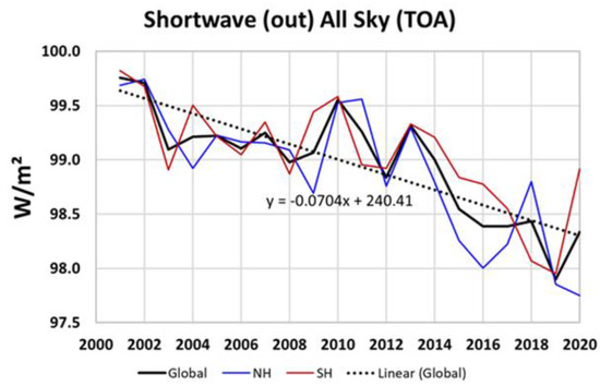
“… the root cause for the positive TOA net flux and, hence, for a further accumulation of energy during the last two decades was a declining outgoing shortwave flux and not a retained LW flux. ” – Hans-Rolf Dübal and Fritz Vahrenholt, October 2021, journal Atmosphere, Radiative Energy Flux Variation from 2001–2020.
What is obvious to any rational person is the recent warming was due to a reduction in clouds that occurred when the PDO went positive in 2014. Without that perfectly natural change the original pause would still be ongoing.
TheFinalNitwit is, as ever, wrong. The correct conclusion to be drawn from the fact that there are so many periods of seven years without warming in the UAH record is that it indicates the overall rate of warming may be – as in fact it is – a great deal less than the fabricators of the climate scam had originally and “confidently” predicted.
There is another pause on horizon so far not predicted by climate models
“Rising lithium prices risk pushing electric car dreams off the road
https://www.telegraph.co.uk/business/2021/11/07/electric-cars-get-expensive-battery-costs-soar/
Somebody beat them to it:
Retailers make shocking petrol profit, says RAC
https://www.bbc.co.uk/news/business-59508286
Quote from the BBC link:”In response to concerns about the Omicron variant, oil prices fell by around $10 a barrel last week.
Typically in the UK market, $1 per barrel usually equates to 1pence per litre
edit: Why does your CR/LF (new line) disappear when you add links
This analysis is very cheering adding as it does to the 1000 year pause estimated from tree ring data for the hockey stick; but it will not stop the Greens, Boris Johnson, the Socialists, the Lib Dems et al from closing the North Sea oil and gas fields. We can only hope that when gas fired central heating is no longer available global warming will be sufficient to keep us cosy in Winter
“Last month I wrote that Pat Frank’s paper of 2019 demonstrating by standard statistical methods that data uncertainties make accurate prediction of global warming impossible was perhaps the most important ever to have been published on the climate-change question in the learned journals.”
I fear Lord Monckton’s memory is playing tricks again. There was no mention by him last month of Pat Frank’s paper – it was carlo, monte who introduced me to his weird statistics, which involves failing to take into account the sample size when estimating uncertainty, as well as some other problems.
I’ll let readers judge for themselves how well slapped anyone down.
The thread starts here:
https://wattsupwiththat.com/2021/11/09/as-the-elite-posture-and-gibber-the-new-pause-shortens-by-a-month/#comment-3385744
and Pat Franks comments start here
https://wattsupwiththat.com/2021/11/09/as-the-elite-posture-and-gibber-the-new-pause-shortens-by-a-month/#comment-3386470
I admire your patience, Bellman. But maybe not so much your time management. Note that Nick Stokes no longer pig fights over this. He prevailed so soundly a couple of years ago that this silliness almost never appears any longer in superterranea. Just check the “Article Impact” of the paper that Pat Frank finally got snuck in after a decade of trying, and about a dozen rejections. 2 citations. One from a chem buddy, one irrelevant.
I thank the Imaginary Guy In The Sky that Bizarro World is actually recognized as such…
Citations are not a judgment of anything except consensus, which is no judgement on scientific soundness. Pat Frank is right, and people who are illiterate on error analysis are wrong.
Exactly. The opinion of Nitpick Nick is not worth the electrons used to compose it.
Thanks, and you are probably right, I wasted far to much time going over this last month. I hadn’t realised this paper had already been debunked by Stokes.
In my defence I’m not really trying to convince anybody, I just do it for my own interest.
Bellman,
You have – at last – gained my interest. If you really do know of an example which shows a paper being debunked by Nick Stokes then I want to see it. (In the days when I often posted here I had much fun using Stokes as an intellectual punch-bag because a ‘battle of wits’ with him was like taking on an adversary in a gunfight who was armed only with a tooth brush.)
Richard
“If you really do know of an example which shows a paper being debunked by Nick Stokes then I want to see it.”
This is such an easy aks that Bellman will let his chauffeur handle it. I hope you don’t mind if it also includes the critique by prominent denier Roy Spencer.
Would you then plz tit for tat us and link us to those Big Foot exchanges where you outsmarted Nick Stokes? But I’ll bone throw. Nick makes his points and then let’s us reflect. He has no control over how many comb overs they fly over. Most, if are actually thought thru, tear up the referenced post in toto, but are instead dismissed as “nitpicking” by those whose thinking conveniently stops when their prejudgments have been “validated”.
https://andthentheresphysics.wordpress.com/2019/09/08/propagation-of-nonsense/
https://andthentheresphysics.wordpress.com/2019/09/10/propagation-of-nonsense-part-ii/
https://moyhu.blogspot.com/2019/09/another-round-of-pat-franks-propagation.html
https://www.drroyspencer.com/2019/09/critique-of-propagation-of-error-and-the-reliability-of-global-air-temperature-predictions/
bigoilbob,
On the basis of Bellman’s contributions to this thread I conclude you are probably right when you say his “chauffeur” could do as well.
However, if you intended to say you are his “chauffeur” then your post proves my conclusion is wrong.
Your bafflegab proves nothing, and I would welcome an explanation of how you think your links support an assertion that Nick Stokes “debunked” Pat Frank because – having read your links – I have seen no evidence of the assertion.
Richard
The furtively pseudonymous “bigoilbob”, like all trained and paid climate Communists, links to four dubious sources, without evaluating their merits (or, rather, lack thereof), as though they demonstrate anything other than a striking ignorance of elementary statistical method on the part of the commentators.
Dr Roy Spencer is considered a dubious source now?
Did you divine this insane conclusion from your Magic 8 Ball?
It’s very easy to see the logic I used to reach my sarcastically “insane” conclusion. You could probably figure it out for yourself if you followed the thread.
Is that clear enough for you, or do I have to draw some pictures?
I don’t open kooklinks as a rule.
Fine, so Dr Roy Spencer is not just a dubious source, but is now a kook.
I’m not actually disagreeing entirely, he’s posted a lot of stuff I find dubious. But it’s good to see you refuse to open any link that you might disagree with. Have to admire your skepticism.
No, blob is. And Spencer doesn’t understand uncertainty any better than you lot.
I see no reason to single out Spencer. Christy, Norris, Braswell, and Parker are listed as authors on the UAH “error estimates” publication.
Only because you don’t WTH yer yapping about—Spencer is in the same trap as you and bellcurveman, believing that uncertainty is error.
What Spencer did was done correctly. The conclusions are not. Radiosonde data does not have 100% accuracy. Therefore it is not capable of determining uncertainty, only a difference between the two. One wrong instrument having a difference of +/- .25C compared to another wrong instrument doesn’t identify uncertainty.
I didn’t know of it, that’s why I wasted my time arguing about it last month. Having searched for Nick Stokes and Pat Frank I see lots of places where he explains the problems – bigoilbob has provided some links below, I see.
Most of the articles are actually about a different paper about uncertainties in modelling, rather than the one we were discussing last month about the uncertainties in HadCRUT data, but the mistakes seem to be of a similar order.
I must say I’m a little annoyed with myself for not seeing this sooner. I’ve spent the last few months trying to explain basic statistics to a few here, and I see last year Nick Stokes made the same points much more clearly than I did. And still nobody was prepared to understand. On the other hand, I do feel I’ve learned quite a bit over the last few months, so it hasn’t all been a waste of time.
It might help if you actually knew some basic statistics.
Basic statistics is your hammer. And you believe that hammer will work on anything. Nothing could be further from the truth.
70 +/- 0.5
40 +/- 0.5
What is their average? What is the uncertainty associated with their average?
Show us your basic statistics and how it works on just these two values.
Using GUM (10)
x_1 = 70
x_2 = 40
u(x_1) = 0.5
u(x_2) = 0.5
f(x_1, x_2) = (x_1 + x_2) / 2
f(70, 40) = 55
∂f/∂x_1 = 1/2
∂f/∂x_2 = 1/2
u_c(Y) = sqrt(Σ[(∂f/∂x_i)^2 * u(x_i)^2, 1, N]) # GUM (10)
u_c(Y) = sqrt((1/2)^2 * 0.5^2 + (1/2)^2 * 0.5^2)
u_c(Y) = 0.3536
Therefore
(70±0.5 + 40±0.5) / 2 = 55±0.3[5]
Using Taylor (3.9) and (3.16)
a = 70
b = 40
δa = 0.5
δb = 0.5
B = (1/2)
q_c = B*a + B*b
q_c = (1/2) * 70 + (1/2) * 40 = 55
q = |B|*x # Taylor (3.9)
δq_a = (1/2) * 0.5 = 0.25
δq_b = (1/2) * 0.5 = 0.25
δq_c = sqrt[δq_a^2 + … + δq_z^2] # Taylor (3.16)
δq_c = sqrt[0.25^2 + 0.25]
δq_c = 0.3536
Therefore
(70±0.5 + 40±0.5) / 2 = 55±0.3[5]
Using Taylor (3.47)
a = 70
b = 40
δa = 0.5
δb = 0.5
q_c = (a + b) / 2
q_c = (70 + 40) / 2 = 55
∂q_c/∂a = 1/2
∂q_c/∂b = 1/2
δq_c = sqrt[(∂q_c/∂a*δa)^2 + … + (∂q_z/∂a*δz)^2]
δq_c = sqrt[(1/2*0.5)^2 + (1/2*0.5)^2]
δq_c = 0.3536
Therefore
(70±0.5 + 40±0.5) / 2 = 55±0.3[5]
Using NIST Monte Carlo method
x0 = 70 uniform σ = 0.5
x1 = 40 uniform σ = 0.5
y = (x0+x1)/2
u(y) = 0.354
Therefore
(70±0.5 + 40±0.5) / 2 = 55±0.3[5]
Conclusion
I performed 4 different calculations using 4 different methods documented by the GUM, Taylor, and NIST. I got the exact same result each time.
You don’t calculate it this way.
if f(x, y) = z = (x+y)/2
then the uncertainty is
u_z = sqrt[ ((δf/δx) * u_x )^2 + ((δf/δy) * u_y)^2 + 0 ]
(uncertainty of 1/2 = 0)
so you get u_z = sqrt[ (1*.5)^2 + (1 * .5)^2] = sqrt[ 0.5] = 0.7
remember the quotient rule.
if q = (x+y)/(w+z) then δq = sqrt[ δx^2 + δy^2 + δw^2 + δz^2]
If w is a constant and z is a constant then their uncertainties = 0.
And you get q = sqrt[ δx^2 + δy^2]
This doesn’t change if you use the expanded form with the partial derivatives. The only time an uncertainty would be multiplied would be if you had q = x^2 + y or something similar. Then the partial would be 2 and you would multiple the uncertainty of x by 2.
Using your notational style:
f(x, y) = z = (x+y)/2
u_z = sqrt[((δf/δx) * u_x )^2 + ((δf/δy) * u_y)^2 + 0]
Then
δf/δx = 0.5
δf/δy = 0.5
Therefore
u_z = sqrt[(0.5 *.5)^2 + (0.5 * .5)^2] = sqrt[0.125] = 0.354
The mistake you made was when you said δf/δx = 1 and δf/δy = 1. That’s incorrect. It is actually δf/δx = 0.5 and δf/δy = 0.5.
Nope. You evaluate uncertainty element by element. Those elements are x, y, and 1/2, not x/2, y/2.
Like I said, look at Taylor’s rules for determining the uncertainty of products and quotients. See equations 3.18 and 3.19.
TG said: “Like I said, look at Taylor’s rules for determining the uncertainty of products and quotients. See equations 3.18 and 3.19.”
Taylor (3.18) is when you multiple or divide measurements each with their own uncertainty. N is not a measurement nor does it have uncertainty. Therefore Taylor (3.18) does not apply. It even says it right there…literally…“Suppose that x, …, w are measured with uncertainties δx, …, δw”.
Do you think N is a measurement? Do you think N has an uncertainty? And when N=2 do you think 1/N = 1/2 is a measurement which has an uncertainty?
Stop obsessing about my hammer.
“70 +/- 0.5
40 +/- 0.5
What is their average? What is the uncertainty associated with their average?”
Depends on what you are trying to do.
1) if these are two measurements and you want an exact average of the two, the average is 55 and the uncertainty is either 0.5 / root 2 ~= 0.4, assuming independent random uncertainties, or at most 0.5.
2) If you are trying to get the mean of a larger population, then a sample of two is not very good, but assuming a random sampling, the mean is still 55. The standard error of the mean, ignoring the uncertainties of the measurements for a moment the standard error of the mean,is still given by standard deviation of the sample divided by root 2, which is approximately 15. As to the measurement uncertainty we could look at each as an error around the true value of the individual measurements, so the average would be the same as in 1) above. Let’s say to be on the safe side its 0.5. Adding these together I would say the estimate for the population mean was 55 ±16.
However you could argue that if the measurement errors are independent of the individual samples, then the actual uncertainty would be √(15² + 0.5²) ~= 15.
As I keep saying, usually measurement uncertainties are trivial compared to the uncertainties from sampling.
You need to provide a reference for this.
You have said you are dealing with a sample. Here are references for dealing with a sample of a population.
=========
https://www.investopedia.com/ask/answers/042415/what-difference-between-standard-error-means-and-standard-deviation.asp
================
https://www.ncbi.nlm.nih.gov/pmc/articles/PMC1255808/
“Now the sample mean will vary from sample to sample; the way this variation occurs is described by the “sampling distribution” of the mean. We can estimate how much sample means will vary from the standard deviation of this sampling distribution, which we call the standard error (SE) of the estimate of the mean. As the standard error is a type of standard deviation, confusion is understandable. Another way of considering the standard error is as a measure of the precision of the sample mean. “
=================
https://stattrek.com/sampling/sampling-distribution.aspx
============================
A distribution of sample means should be normal by the central limit theory. It does not matter what the shape of the population is, by the CTL the sample mean distribution will become normal. This is somewhat dependent on sample size and number of samples.
Here is a reference for the above.
From:
https://guides.fscj.edu/Statistics/centrallimit
It should be obvious that if the sample means distribution and the population distribution are not the same, that each should have different standard deviation.
The SEM is calculated by the formula:
SEM = SD / sqrt N, where N is the sample size.
The first observation of this formula is that the SEM is always smaller, not larger than the SD of the population.
The second observation is that the SEM gets smaller as the sample size increases. This implies that the sample means distribution gets more and more narrow as the sample size approaches the size of the population.
One should notice that dividing a sample means distribution standard deviation (SEM) will give you nothing. At best you will get the sample means standard deviation of a sample of a sample. You could continue to do this until it converges on zero. However, since the CTL says you should have a normal distribution with taking the first sample, statistically, you gain nothing.
“You need to provide a reference for this.”
Have you tried reading a basic stats text book, or looking on the internet, or read the comments I’ve sent to Time?
Here for example:
https://wattsupwiththat.com/2021/12/02/the-new-pause-lengthens-by-a-hefty-three-months/#comment-3406089
We estimate the standard deviation of the population, by taking the sample standard deviation. Here as the sample is just two this is √[(70 – 55)² + (40 – 55)²] = √(2*15²) = 15*√2.
Net you divide by √2 to get the SEM. Can you guess what that is?
What I probably should have mentioned, is that to use this for a confidence interval you need to use the 1 degree student-t distribution, which will be somewhat larger than than a normal one given the small sample size. For example, if you want a 95% confidence interval you would need 15*12.7 ~= 191. (If I’m remembering how to do this correctly). So if we are using extended uncertainty the mean is
55 ± 191
Which makes the ±0.5 uncertainty from the measurements even less interesting.
https://byjus.com/maths/standard-error-of-the-mean/
Why yes I have. I even have its text stored in a file. Here is what this reference says that contradicts your divide by the √2 to get the SEM.
I am sure what threw you off track was the example shown. You need to stop just cherry picking things that you google. If you don’t take the time to study some textbooks and learn the basics of statistical sampling you will never know the assumptions of how this works. There are several good youtube lessons about this.
Please note that this is NOT a sample. It is the population of data. Therefore the SD is the standard deviation of the population.
They go to show what the standard error of the mean, SEM is.
You keep showing so little understanding, or ability to read. FYI, I’ve been trying to explain how to estimate a SEM from a sample for months. It’s not exactly hidden knowledge, it’s pretty well known. I only searched for internet pages as I though you might be able to understand them better. But as always I fail to understand just how deep the cognitive dissonance goes.
Note that particular page doesn’t even make a distinction between population and sample deviation, which is a bit of unfortunate.
“Please note that this is NOT a sample. It is the population of data. Therefore the SD is the standard deviation of the population. “
No it isn’t. If it were, there would be no point in finding the SEM, you already know the mean. Point two, if it were the population they wouldn’t be working out the sample standard deviation – that is dividing by (N-1), they would be working out the population standard deviation, dividing by N.
Now try the next site on my search
https://www.scribbr.com/statistics/standard-error/
When population parameters are unknown
(My emphasis)
The formula, of course, is
where s is the sample standard deviation.
Here’s another one that shows up in my search, a calculator that will let you put in any sample sized sample and not only gives you an answer, but shows the workings.
https://ncalculators.com/statistics/standard-error-calculator.htm
It also gives these instructions to estimate the Standard Error
1. Estimate the sample mean for the given sample of the population data.
2. Estimate the sample standard deviation for the given data.
3. Dividing the sample standard deviation by the square root of sample mean provides the standard error of the mean (SEM).
Mr Stokes did not “prevail”. He made a number of characteristically ignorant and deceptive comments on Dr Frank’s paper, which remains unsullied. Besides, as the head posting makes clear, it is only because climatology makes the elementary control-theoretic error of ignoring the feedback response to emission temperature, effectively adding it to and miscounting it as part of the actually minuscule feedback response to warming directly forced by greenhouse gases that it imagines it can predict global warming accurately.
“Mr Stokes did not “prevail”.”
Mr. Stokes, Dr. Spencer, and all the others who, mostly independently, documented the silliness of Pat Frank’s paper did indeed “prevail”. Thankfully, they demonstrated it’s fundamental flaws well enough to wave off other scientists who instead chose valid sources in citations. And since science advances via learning from others, Nick et,. al. did us a solid by keeping us pointed in the right direction. It is the scientific version of the oft used Simpson’s scene. Homer says something so ridiculous that after a long pregnant pause, Maggie changes the subject and Homer is left to rant in WUWT, and link to his (again, thankfully) unused paper.. Sorry, mixing metaphors.
As for the rest of your comment, pregnant pause starts here. Along with incredulity that your repeated “pause” posts, using statistically/physically insignificant time periods, have any actual validity.
Bob:
Do you see how it works in Monckton’s world?
He just says stuff …. And therefore it’s true!
Like a lot of what passes for science on here.
It’s true because he says so, or because the attack-dogs have piled in and shouted down the criticism.
That passes for a “win” here.
It’s what happens down the rabbit-hole as “peer-review”.
Never address your critics and swear-blind you are correct.
Sorry Monckton, that’s not how peer-review of science works.
That is Mr Franks MO as well …. Oh and Heller’s too.
Also, how can there be a pause in place in the UAH V6 when
the long-term warming trend of said series is still increasing!
That purported “pause” lies at a warmer level that the LT trend.
It beggars belief, but then so does the pizza-parlour peodophile gang and look how that panned out!
It’s amazing what group identity and cognitive dissonance does to peoples common-sense – and how dangerous it can be (in that case).
Well done M’Lord – you are selling a great snake-oil recipe with this one …. And denizens unthinkingly fawn on you ….. which is of course why you continue.
Again – Why satellite data misses much of the surface warming …
It’s a slice of the atmosphere well above the surface – that continues to warm at a rate not seen by the satellite due to its inability to see into a surface inversion, where nocturnal minima are increasing and which is the chief AGW component over land.
No spaghetti today, Baton?
The poisonous Mr Banton, yet another paid climate Communist who knows no science but is pathetically faithful to the Party Line, has not the slightest idea whether Dr Frank is right or whether his fellow climate Communists such as Mr Stokes are right. But he knows that the Party Line requires. Pathetic! Vapid! Apolaustic!
Here is a summary of some of my concerns regarding the Frank 2010 publication.
1) His use of sqrt(Nσ^2/(N-1)) is inconsistent with the formula defined in the GUM and with results from monte carlo simulations provided by NIST for this type of uncertainty propagation.
2) He does not propagate the observed temperature uncertainties through a global grid mesh which every datasets employs. It was not clear to me that he understood that global mean temperatures are calculated by via averaging the grid mesh as opposed to averaging the stations directly.
3) This is really an extension of #2, but he makes no mention of the degrees of freedom of the grid meshes. For example, UAH has 9504 cells, but only 26 degrees of freedom due to the sampling strategy of the satellites. A similar DOF analysis would need to be performed on the 2592 cell grid that HadCRUT uses, 8000 cell grid that GISTEMP uses, the 15984 cell grid that BEST uses, the ~500,000 cell grid that ERA uses, etc. You can’t assume N is the number grid cells because of spatial error correlations. The DOF will be lower than the number of grid cells.
4) This is another extension of #2, but he makes no mention of the uncertainty arising from the various grid cell infilling techniques. For example, BEST quantifies this uncertainty (including other kinds of uncertainty) via the jackknife resampling method.
5) He uses Folland 2001 of 0.2 and Hubbard 2002 of 0.25 (technically he used 0.254 from his own calculated Guassian distribution based on Hubbards research) as starting points for the analysis. He claims neither has a distribution despite Folland calling it a “standard error” and Hubbard straight up publishing the distribution.
6) He combines the Folland and Hubbard uncertainties even though they seem to be describing the same thing. The difference is that Folland is terse on details while Hubbard is verbose.
And you are still wrong, as Pat tried to tell you in October. But, on a positive, you revealed yourself as a shill for the IPCC propaganda.
Did Pat or you ever give a reference for how to propagate “assigned” uncertainties?
For the record, I have no affiliation with the IPCC.
bdqwx,
For the record, I believe you.
Richard
Notice that did not write that you did have an affiliation, only that you shill for the IPCC propaganda.
You used the word “shill”. Wikipedia defines that as “a person who publicly helps or gives credibility to a person or organization without disclosing that they have a close relationship with said person or organization.” I don’t have a close relationship with the IPCC.
BFD—the point is you defend the political garbage put out by those people; whether you have a membership card or not is irrelevant.
I don’t defend or attack “political garbage” either. I hate politics regardless of whether it is garbage or not with a passion so if you want to steer the discussion down that path I’ll respectfully bow out.
bdgwx,
The UN IPCC only deals in “political garbage” (i.e. propaganda) because it is the InterGOVERNMENTal Panel on Climate Change and everything done by any government(s) is political.
Richard
Bingo—finally someone pointed at the elephant inside the tent.
Good list.
One think that’s been puling me, is why he combines the uncertainty of the base period and the temperature to get the uncertainty of the anomaly. If you are looking at the trend, any uncertainty in the base period is irrelevant as it will be a constant.
Just divide by root-N and all yer problems disappear in a puff of greasy green smoke.
If only.
You still ignore what happens to your fantasy when the sampling rate is upped.
Oops.
What are you on about this time? You are beginning to sound like a bad automatic insult generator.
I’m not ignoring what happens when you increase sampling, that’s the main objection to Pat Frank’s paper. He assumes the uncertainty is the same regardless of the sample size – hence there’s no less uncertainty in 1850 than there is in 2000. This is at least a bit more realistic than the original claim here that uncertainty increases with sample size.
Have fun inside your house of mirrors.
So what do you think happens when the sampling rate is “upped”?
You have to find another way of combining the individual variances, as I’ve been futilely attempting to inform you.
The baseline is made up from measurements is it not? Therefore there will be uncertainty in the baseline value.
Don’t you know? Subtraction removes ALL errors!
My point was that as far as the trend is concerned it isn’t. That’s why it doesn’t matter when UAH keeps changing the baseline every decade. The values change but by equal amounts.
It’s different if you are looking at the anomaly in it’s own right. If you are saying November was 0.08°C above the 1991-2020 average. This may be wrong because the November 2021 was wrong, or it might be wrong becasue the 1991-2020 average is wrong, or a combination of the two. But no matter how wrong the baseline is, it will not affect the trend.
Hey Señor Experto, what are the raw monthly UAH temperature values before the subtraction? Why aren’t these published?
They are published. Well at least the 1991-2020 baseline is. You can add the monthly anomalies to the baseline to get the raw temperature. For example, the November baseline is 263.406 K which means the November 2021 raw temperature is 263.490 K. And before you start gripping about significant figures understand that I’m providing the values as reported by UAH so you can take up this issue with Dr. Spencer and/or Dr. Christy.
From your link:
-9999-9999-9999-9999-9999-9999-9999-9999-9999-9999-9999-9999-9999-9999-9999-9999
-9999-9999-9999-9999-9999-9999-9999-9999-9999-9999-9999-9999-9999-9999-9999-9999
-9999-9999-9999-9999-9999-9999-9999-9999-9999-9999-9999-9999-9999-9999-9999-9999
-9999-9999-9999-9999-9999-9999-9999-9999-9999-9999-9999-9999-9999-9999-9999-9999
24668246592465624669246822467924692246802469624687246892467124661246672467424650
24663246412462124610245682455624541245032446324434243842432724280242052415824104
24107241132412224204242472434124419245062456824611246492463624649246712466524665
24667246742465724667246432463324652246202458824563245182448424451243842434724329
24272241962412724078240082398323942238942383323773237082365823641235942354523519
23471234042334923296232322318623131230712302022980229132284822826227912275122733
22723227012267222669226362263122618226212260922634226562269922718227552277122838
22880229042293823022230642310523173232062327323321233382338723411234932356823637
Oh yeah, this is convincing…not.
And you didn’t answer my question, no surprise.
If you’re question isn’t concerning the raw absolute UAH TLT temperatures then what are you asking for?
Are you daft? I asked WHY aren’t they published, and you gave me a link to a bizarre page filled with indecipherable numerology.
The link I gave you is literally the gridded raw absolute temperatures. It is a 2.5×2.5 lat-lon grid with 10384 grid cells on which only 9504 are filled. The -9999 values are the cells that UAH does not estimate. Each value is 5 characters in units of 1/100 K. For example, the first filled cell is 24668 which is 246.68 K. Each latitude ring is represented by 9 rows in the file. The global mean mean temperature is the area weighted average of the 9504 filled grid cells. That means the 10384 cell area weighted average treats the 880 unfilled cells as if they inherit the average of the 9504 filled cells.
Why did you leave this information out?
What are the uncertainties of each value?
Where are the monthly values?
246K = -26°C, hmm interesting number
I was assuming you would be able to figure it out.
Uncertainty is assessed in Christy et al. 2003.
The monthly values are in that file.
That is the value for the first cell on the lat=81.25N ring.
More crapola—all that paper does is compare the Holy Trends, it is not an uncertainty analysis.
Funny thing— only a few temperatures in that huge list are greater than 0C—does this bother you?
The publication estimates the uncertainty on monthly and annual temperatures both at a specific location and on a global scale. It also estimates the uncertainty on the trend. If you have an issue with it I recommend you contact Dr. Spencer. He does respond to questions on his blog.
No it doesn’t. Why is that funny? Why should the fact that only a few temperatures being greater than 0C bother me?
It is already well established that you are not an honest person—once again, that paper is not an uncertainty analysis. All it does is compare against radiosonde data.
Did you even read it?
Yes I’ve read it. That’s how I know the assessed uncertainty is ±0.20 C for monthly global mean temperatures. That literally makes it an assessment of uncertainty. The fact they use radiosonde data does not mean they weren’t assessing uncertainty. It just means (presumably) that you didn’t like the way they did it. I’ll be honest I have concerns with their methodology as well. I think the technique Mears used is more robust. I’m not an expert though so I make no statements on the quality of these assessments except that I have no heard of any egregious mistakes with them. If you know of another assessment I’d be happy to review it.
And I’m telling you this is absurdly small bullsh!t on the surface. If you can’t see this I can’t help you.
You have absolutely no clues about what a real UA is.
I’m not saying it is right. I’m just reporting what Dr. Christy and Dr. Spencer say.
It’s not for the surface. It’s for the UAH TLT layer which is essentially the entire depth of the troposphere with the weighting peaked at around 700mb.
I thought it was a rather large uncertainty for a global mean. The surface dataset are on the order of ±0.05 C.
milliKelvin? Are you serious? The thermometers are no better than 0.5C and likely more like 0.9-1.0C, how in the world do you get an order-of-magnitude better?
For the modern era Hubbard 2002 says ±0.25 for daily average temperature at a single station. Per the GUM ±0.25 would be the upper bound on the combined uncertainty if all measurements were perfectly correlated. If all measurements were perfectly independent you’d probably be on the order of ±0.001 or lower. The reality is that there is neither perfect correlation nor perfect independence. This puts the real world combined uncertainty somewhere in between. The exact value depends on methodology used like station processing, grid meshing, temporal sampling strategy, spatial sampling strategy, constrain analysis (like what reanalysis does), etc. and on the number of observations used. Different datasets publish different uncertainty estimates. ±0.05 C is a reasonable order of magnitude estimate at least for the post WWII era.
I don’t care who Hubbard is or what his nonsense claims are, all this fluff you dump into the air is utterly without any coherent meaning.
If the Hubbard 2002 conclusion is nonsense then the Frank 2010 conclusion of σ = 0.46 is nonsense.
Yeah, Pat saw through your act in about 4 posts.
Perhaps I should make my point clear. Frank 2010 depends on Hubbard 2002 and Folland 2001 being correct. Those are the only two lines of evidence that form the entirety of the the 0.46 value.
Here are the calculations. 1a uses 0.2 from Folland 2001 and 2a uses 0.254 from the Hubbard 2002 distribution. Note that N is a large number.
(1a) sqrt(N * 0.2^2 / (N-1)) = 0.200
(1b) sqrt(0.200^2 + 0.200^2 = 0.283
(2a) sqrt(N * 0.254^2 / (N-1)) = 0.254
(2b) sqrt(0.254^2 + 0.254^2) = 0.359
(3) sqrt(0 283^2 + 0 359^2) = 0.46
If you think Hubbard 2002 is nonsense than the result in (3) of 0.46 is also nonsense.
NO! The paper calculated a minimum uncertainty, using numbers put out by AGW-heads. Considering that the best thermometers available have accuracy specs on the order of ±0.5°C, it easily could be larger! And most likely is as 0.5°C is only the RTD sensor itself.
But do continue in your milli-Kelvin fantasy world, don’t let me get in the way.
For people who are obsessed with air temperature, it is quite amazing to see how little y’all know about real measurements.
My point is that if the input quantities 0.2 and 0.254 are both nonsense then the output quantity 0.46 must also be nonsense. Have you expressed your concerns with Frank regarding his choice of inputs?
No, the point is yer an idiot who doesn’t have a single about reality, especially measurements, yet somehow think that you do.
Hardly. He wasn’t very responsive with my questions. In particular I asked him about propagating the uncertainty through the HadCRUT grid mesh. His response was odd and made me immediately question whether he even understood how HadCRUT estimates the global mean temperature. He seemed to imply that they just do a straight average of the monthly station anomalies which couldn’t be further from the truth. He never would explain what the Folland 2001 figure of 0.2 meant despite having no qualms in using it. He claimed that the Hubbard 2002 figure of 0.254 had no distribution despite literally calculating the value from the Guassian distribution that Hubbard provided.
Because you are completely unable to form meaningful coherent questions. He saw through your act in about 4 posts.
“If the Hubbard 2002 conclusion is nonsense then the Frank 2010 conclusion of σ = 0.46 is nonsense.”
You still don’t understand metrology at all. Pat’s work was based on extending specific measurement data. Hubbard and Spencer was based on comparing the outputs of two different sets of instrument and assuming one was 100% accurate.
You don’t know enough about the subject to understand any of this. You are still cherry picking stuff trying to rationalize your view of the subject instead of actually learning about it.
If the calibration requirement for US measurement stations is +/- 0.6C (see the Federal Meteorology Handbook No. 1) then the average temperature uncertainty simply can’t be +/- 0.25C.
Again, Hubbard did the same thing that Spencer did with the satellite record. They compared their results to a REFERENCE and calculated the average difference betweeen the two while ignoring the uncertainty of the reference.
They each made an unsupported assumption that their reference was 100% accurate with no uncertainty.
No, you wouldn’t. The uncertainty would be on the order of +/- 1.2C.
The reality is that the correlation is less than 0.8 between most stations. The correlation is based on cos(φ) where φ is a function of distance, elevation, pressure, terrain, and probably others like wind and the substance below the measurement site. A 50mile distance alone puts the correlation below 0.8 – which is considered uncorrelated by most.
That means most temperatures will be independent. The uncertainties of any sum of the temperatures will add either directly or by root-sum-square.
“ ±0.05 C is a reasonable order of magnitude estimate at least for the post WWII era.”
Total and utter malarky. LIG thermometers were still in use long after WWII. Their minimum uncertainty was more like +/- 0.5C to +/- 0.25C.
Averages do *NOT* reduce uncertainty!
TG said: “Again, Hubbard did the same thing that Spencer did with the satellite record. They compared their results to a REFERENCE and calculated the average difference betweeen the two while ignoring the uncertainty of the reference.”
If the Hubbard 2002 value of 0.25 is wrong than the Frank 2010 value of 0.46 is also wrong.
TG said: “Averages do *NOT* reduce uncertainty!”
Did you perform the procedure in section 5 of the GUM before making that assessment? Can you show your work?
As you were told yesterday (and ignored) Pat used the numbers generated by the AGW crowd and demonstrated they lead to u(T) no less than 0.46°C for these averages.
Why do you sweep uncertainty under the carpet?
That doesn’t make it any less wrong. If the correct value that should have been used in place of the Hubbard 2002 value were lower then the 0.46 figure computed by Frank 2010 would be lower thus a statement of “no less than 0.46” would be wrong.
Nitpick Nick Stokes should be proud.
The point is, which you continue to ignore, the GAT uncertainty is likely a lot larger than 0.46°C.
Not if the Hubbard 2002 0.25 is lower. If Frank 2010 were to dismiss Hubbard 2002 then what other line of evidence could be used in it’s place for the MMTS uncertainty?
The average is (x_1 + x_2+ … + x_n)/n
Thus total uncertainty is u_t = δx_1 + δx_2 + …. + δx_n + δ(1/n)
Since n is a constant then δ(1/n) is zero.
So the total uncertainty is the sum of the uncertainties of the values in the data set.
If you want to use RSS that’s ok. But the uncertainty will still be based on the uncertainties of the data points and not on the number of the data points.
TG said: “Thus total uncertainty is u_t = δx_1 + δx_2 + …. + δx_n + δ(1/n)”
That’s not what Taylor (3.9), Taylor (3.16), Taylor (3.47), GUM (10, and the NIST uncertainty machine say.
“That’s not what Taylor (3.9)”
You can’t read any better than Bellman!
==================================
Taylor 3.9:
Measured Quantity times Exact Number
If the quantity x is measured with uncertainty δx and is used to compute the product fq = Bx,
where B has no uncertainty, then the uncertainty in q is just |B| times that in x,
δq = |B|δx.
===========================
A fraction in this case makes no sense. Look at the explanation Taylor gives after stating 3.9 =>
“This rule is especially useful in measuring something inconveniently small but available many times over, such as the thickness of a sheet of paper or the time for a revolution of a rapidly spinning wheel. For example, if we measure the Thickness T of 200 sheets of paper and get the answer
(thickness of 200 sheets) = T = 1.2 +/- .01 inches.
It immediately follows that the thickness of a single sheet is
(thickness of one sheet) = t = 1/200 x T
= .0065 +/- .0005 inches.
=====================================
Tell me why you would divide δt by 1/B in order to find δq.
You *HAVE* to read for meaning and understanding instead of just cherry picking something you think is useful. If you had read what Taylor says after the rule you would have MAYBE understood what the rule means.
Taylor’s 3.16 is not even on point for the subject!
Uncertainties in Sums and Differeneces.
Suppose that x, …, w are measured with uncertainties δx + … + δw and the measured values are used to compute
q = x + … + z – (u + … + w)
If the uncertainties in x, …, w are known to be independent and random then the uncertainty in q is the quadratic sum
δq = √ [(δx)^2 + … + (δz)^2 + (δu)^2 + … + (δw)^2]
of the original uncertainties. In any case, δq is never larger than their ordinary sum
δq = δx + … + δw
=====================================
There is no division by a constant in this calculation of uncertainty.
3.47 is no different than 3.9 other than the use of partial differentials when q is a function of (x, … z)) instead of a sum of (x + … + z).
None of these prove anything about your assertion that uncertainty doesn’t grow with more independent, random data values.
All your post proves is that you can’t read and can’t do basic math. You are a troll, nothing more. You know nothing, absolutely nothing of metrology. All you have are some cherry picked equations which you continually misuse and misrepresent. Have you no shame?
TG said: “Tell me why you would divide δt by 1/B in order to find δq.”
t = B * T where t is the thickness of a sheet, T is the thickness of the stack and B is the number of sheets.
And per (3.9):
δt = |B| * δT
So
t = 1/200 * 1.3 = 0.0065
δt = |1/200| * 0.1 = 0.0005
TG said: “Taylor’s 3.16 is not even on point for the subject!”
You can use (3.16) in tandem with (3.9) to determine the uncertainty of a combined quantity where each input quantity is itself a simple combined quantity using the exact number rule (3.9).
TG said: “3.47 is no different than 3.9”
Taylor 3.47 is the same partial differential method as GUM (10). The partial differential of f wrt to both x and y is 1/2 when f = (x+y)/2.
“t = B * T where t is the thickness of a sheet, T is the thickness of the stack and B is the number of sheets.”
Did you read this before you posted it?
You just multiplied the thickness of the stack, T, by 200 in order to get the thickness of each sheet, t.
Normally “t”, the thickness of a sheet, would be less than “T” the thickness of the stack. Are you trying to do some funky kind of origami?
The rest of your post on this follows the garbage you start with. This idiocy *should* point out to *YOU* yourself that you have this all confused!
Nope. You evaluate uncertainty on an element by element basis. Your elements are s, y, and 1/2.
See Taylor’s 3.18 and 3.19 on uncertainties of products and quotients.
You are *still* cherry picking without actually understanding what you are talking about. Your clear misunderstanding stands as proof that you are just cherry picking while not caring about what you are posting.
As long as it supports the idea that GAT uncertainties are tiny, he/they doesn’t care.
TG said: “Did you read this before you posted it?”
Yes I did.
TG said: “You just multiplied the thickness of the stack, T, by 200 in order to get the thickness of each sheet, t.”
No I didn’t. I multiplied the thickness of the stack, T, by 1/200 in order to get the thickness of each sheet, t exactly how Taylor did it on pg. 55…literally…”t = 1/200 * 1.3 = 0.0065″ is what I said.
TG said: “Normally “t”, the thickness of a sheet, would be less than “T” the thickness of the stack. Are you trying to do some funky kind of origami?”
Duh! And no. I’m doing 3rd grade arithmetic here. It’s not that hard. “t = 1/200 * 1.3 = 0.0065” is the correct solution and I stand by what I said even if you don’t agree with it.
And because t = B * T then δt = |B| * δT exactly the way Taylor (3.9) says to do it. B = 1/200. That is an exact number with no uncertainty so Taylor (3.9) applies. Therefore δt = |1/200| * 0.1 = 0.0005.
TG said: “Nope. You evaluate uncertainty on an element by element basis. Your elements are s, y, and 1/2.”
Yes it is. When f = (x+y)/2 then ∂f/∂x and ∂f/∂y are both 1/2. Here let’s do an example together.
x = 1, y = 1 then f = (1+1)/2 = 1
now x by 1 unit
x = 2, y = 1 then f = (2+1)/2 = 1.5
Did you see how f changes by 0.5 when x changes 1?
bdg –> “t = B * T where t is the thickness of a sheet, T is the thickness of the stack and B is the number of sheets.” (bolding mine, tpg)
bdg –> “I multiplied the thickness of the stack, T, by 1/200 in order to get the thickness of each sheet, t exactly how Taylor did it on pg. 55…literally…”t = 1/200 * 1.3 = 0.0065″ is what I said.” (bolding mine, tpg)
B is the number of sheets.
And B is 1/200.
So the number of sheets is 1/200?
I’m done. You ARE a troll. You can’t even be consistent with yourself.
I truly tire of feeding a troll that knows nothing about the subject!
bye-bye!
Ah…yes. That’s obviously a typo. I didn’t even notice it until now. Let me correct that now too.
bdgwx should have said: “t = B * T where t is the thickness of a sheet, T is the thickness of the stack and B is 1 divided by the number sheets.”
While I’m not a troll I am a human who makes more than my fair share of mistakes. Let it be known that I own my mistakes and correct them as quickly as possible.
I know there’s no point trying to pursuade you why this is wrong. But your problem is that you are mixing up the rules for propagating addition and subtraction, with the rules for multiplication and division.
Adding and subtracting quantities means adding absolute uncertainties, multiplying and dividing means adding the fractional uncertainties.
If you could only understand that important distinction you might begin to understand why you are wrong. You cannot simply add zero to the absolute uncertainty of the sum in order to see what happens when you divide the sum by a constant. The effect of adding zero to the fractional uncertainty is to leave it unchanged, which means of necessity the absolute uncertainty has to change.
Nope!
Let q = (x * …. *z) / (u * … * w)
Taylor Eqns 3.18 and 3.19 uncertainty of products and quotients.
ẟq|q| = sqrt[ (ẟx/x)^2 + …. + (ẟz/z)^2 + (ẟu/u)^2 + … + (ẟw/w)^2 ]
In any case, it is never larger than:
ẟq/q ≤ ẟx/x + … + ẟz/z + ẟu/u + …. + ẟw/w
Meaning. if you have (x + y)/2 then x, y, and 2 are all separate elements (e.g. x, z, w) that are added together to get the total uncertainty.
When are you and bdg going to stop cherry picking crap to throw against the wall to see it if sticks and actually start learning the rules for propagating uncertainty?
TG said: “Meaning. if you have (x + y)/2 then x, y, and 2 are all separate elements.”
Patently false. First, x and y are added; not multiplied or divided as mandated by Taylor (3.18). Second, 2 is an exact number with no uncertainty. All variables in Taylor (3.18) must be measurements with uncertainty.
Here is what Taylor says about (3.18).
What do you think ẟx/x means, if not fractional or relative uncertainty?
“Meaning. if you have (x + y)/2 then x, y, and 2 are all separate elements (e.g. x, z, w) that are added together to get the total uncertainty.”
But you’ve got two different operations, and and divide and the uncertainties need to be propagated differently.
You can keep telling us that we’ve cherry picked something all you like, but what we are pointing out is the standard rules for propagating uncertainties, not just in Taylor, but in any account of how to propagate uncertainties.
Here’s the first site I found searching for “propagate uncertainties”. Note in particular the “unofficial” Rule #4.
https://www.cpp.edu/~jjnazareth/PhysLabDocs/PropagateUncertainty.pdf
Rule #1 – Addition and/or Subtraction of numbers with uncertainty
Add the absolute uncertainties.
Rule #2 – Multiplication and/or Division of numbers with uncertainty
Add the relative uncertainties.
Rule #3 – Powers applied to numbers with uncertainty (like squared or square root)
Multiply the relative uncertainty by the power.
(Unofficial) Rule #4 – Multiplying by a number without uncertainty (like ½ or π)
Multiply the absolute uncertainty by the number without uncertainty
Something else no one ever considers is the conversion between F and C.
+/- 0.6C ~ +/- 1F
+/- 0.5F ~ +/- 0.3C
So, for U.S. temps of integer values in Fahrenheit converted to Celsius there is about a +/- 0.3C uncertainty.
A 1.5C increase over the last 150 years would convert to about 3F. We should be setting Tmax records every day in every place!
Like MC stated, the study assumes the radiosonde data is 100% accurate and then they calculated the difference between the satellite values and the radiosonde values and called it “uncertainty”. It’s not uncertainty, it is “discrepancy”.
Why is he now yapping about “perfect correlation” and “perfect independence”? Where did this stuff come from?
He has me baffled.
See GUM section 5. Equation (13) is the general case. When all correlations r(X_i, X_j) = 0 (perfectly independent) then equation (10) can be used. When all correlations r(X_i, X_j) = 1 (perfectly correlated) then the equation in 5.2.2 Note 1 is used.
Go ahead then and use them. Have fun. Idiot.
So Mr. Metrology, do tell exactly where, when sampling air temperature twice a day, hourly, every minute or every second, is the threshold between “perfectly independent” and “perfectly correlated”?
It’s neither perfectly independent nor perfect correlated. That’s what Bellman and I have been trying to explain. That’s why the lower bound on the uncertainty is ψ√N and the upper bound is ψ where ψ is the standard uncertainty of the temperature in each grid cell. Note that I’ll using ψ for the standard uncertainty of u(x_i) for all x_i now instead of σ to respect your annoyance with its use. If ψ annoys you as well no big deal; I’ll be happy to use what ever symbol is acceptable to you.
You ran away from, or didn’t understand, the point: your own equations go to zero with more data points.
Those aren’t my equations. Those equations come from the GUM which you not only told me to use, but said if I didn’t use the GUM then whatever I presented would be useless.
No they aren’t, now you are just a liar.
The only people you are fooling with this act are yourself and bellcurveman.
Where is your correlation matrix calculation? BZZZZT
Try to read (I know, this is tough) the example in 5.2.2 and then bloviate some more about how temperature measurements are “correlated” or not “perfectly correlated”, a term you pulled out of your hindside.
CM said: “No they aren’t, now you are just a liar.”
They are literally in the GUM. See section 5. Section 5.2.2 is the general case. When all correlations r(X_i, X_j) = 0 then section 5.1.2 can be used. When all correlations r(X_i, X_j) = 1 then 5.2.2 Note 1 can be used.
CM said: “Where is your correlation matrix calculation?”
I literally gave it to you my post above.
bdgwx said: “When all correlations r(X_i, X_j) = 0 (perfectly independent) then equation (10) can be used”
and
bdgwx said: “When all correlations r(X_i, X_j) = 1 (perfectly correlated) then the equation in 5.2.2 Note 1 is used.”
CM said: “a term you pulled out of your hindside”
If my terms annoy you then propose different terms. Fill in the blanks.
When r(X_i, X_j) = 0 for all X_i and X_j we mutually agree to call that _____?
When r(X_i, X_j) = 1 for all X_i and X_j we mutually agree to call that _____?
I’ll use whatever terms you are comfortable with (within reason). Just know that it doesn’t change anything whatsoever.
Or you can just blow some more smoke…
I think real world temperatures in the grid cells have r(x_i, x_j) > 0 for all x_i and x_j. Do you disagree?
Where in Eq 13, 16, or Note 1 does it show dividing by N to get uncertainty?
Were in Eqn 10 or 11 doess it show dividing by N to get uncertainty?
When f = Σ[x_i, 1, N) / N then ∂f/∂x_i = 1/N for all x_i. And it’s not “dividing by N”; it’s dividing by the square root of N.
“When f = Σ[x_i, 1, N) / N then ∂f/∂x_i = 1/N for all x_i. And it’s not “dividing by N”; it’s dividing by the square root of N.”
I asked where in Eqn 10/13 1/N appears. I don’t see it.
Eqn 10:

Eqn 13:
Show me the sqrt(1/N).
TG said: “Show me the sqrt(1/N).”
I’ve already done this multiple times. I might as well do it again even though you’ll ask me again tomorrow as well.
GUM (10): u_c(Y)^2 = Σ[(∂f/∂x_i)^2 * u(x_i)^2, 1, N]
To compute an average of all x_i via the function f we let:
f = Σ[x_i, 1, N] / N
so…
∂f/∂x_i = 1/N for all x_i
and if u(x_i) is the same for all x_i then we let:
ψ = u(x_i) for all x_i
then…
u_c(Y)^2 = Σ[(∂f/∂x_i)^2 * u(x_i)^2, 1, N]
u_c(Y)^2 = Σ[(∂f/∂x_i)^2 * u(x_i)^2, 1, N]
u_c(Y)^2 = Σ[(1/N)^2 * ψ^2, 1, N]
u_c(Y)^2 = (1/N)^2 * ψ^2 * N
u_c(Y)^2 = ψ^2 / N
u_c(Y) = ψ / √N
Carlo Monte, are going to fill in the blanks or not so that we can continue discussing GUM section 5.2?
It *does* mean they weren’t assessing uncertainty unless the radiosonde data is 100% accurate! I sincerely doubt that.
And if you read through the paper, they even talk about some of the problems with radiosonde measurements.
yep. and then they go ahead and ignore the problems and use the data as a 100% accurate reference. Again, they calculated the size of the bias between the two data sets, not the uncertainty of each.
Spencer doesn’t do the uncertainty correctly. If he did the uncertainty in the monthly average temp would be greater than what he is trying to discern. If you made your line widths equal to the uncertainty of the temp values you wouldn’t be able to discern any specific trend. It’s the problem of assuming that all the values are 100% accurate – i.e. the temp measurements are not a “stated value +/- uncertainty” they are just “stated value”.
It’s why Spencer didn’t like Frank’s showing how an uncertainty grows over iterative processes.
The idea that temperature is a tough measurement and that getting better than ±1°C is a tough pill to swallow for the Holy Trenders.
The more I think about the UAH calculation (which is a black box to the outside world), I’m thinking that because the calculation procedure is fixed, it might be possible to do a Monte Carlo uncertainty simulation and get an idea of the actual u(T). From what I can tell there would be a lot of parameters to vary so it might not be easy, but could be closer to reality than this 10 mK nonsense.
UAH does not claim 10 mK of uncertainty. They claim 200 mK of uncertainty.
Are you saying an assessment of uncertainty using a monte carlo simulation would be acceptable to you?
Oh yes, here it comes, yer now an expert on Monte Carlo uncertainty assessment now. I knew it.
200mK is still bullshite.
I’ve not done a monte carlo simulation of the satellite temperature uncertainties. I’m just asking if that is an acceptable methodology to you.
Have you ever done any real measurements? Of anything?
Answer: No
Yes, but that is completely irrelevant. You should be able to answer the question of whether a monte carlo simulation assessment of uncertainty is acceptable to you regardless of my answer to your question.
A Monte Carlo simulation can be just as inane as global climate models if the simulation doesn’t contain all aspects of variability.
So is that a no? You would not accept a monte carlo simulation based assessment for satellite based temperature datasets?
CAN YOU READ? No
A MC simulation has to be realistic to be of any value, otherwise it is just more AGW GIGO.
There is no way to answer your diversionary question without someone doing the exercise.
Next…
Then why suggest a monte carlo simulation to assess uncertainty if you won’t accept it anyway?
Yer an idiot—if done carefully with a valid model it can give useful information. It might take 10 years of CPU cycles though.
But you still want to cling to your impossible and absurdly small uncertainties for your Holy Temperature Averages.
It sounds like you’re saying that you’ll accept a line as evidence as long as it meets criteria that is impossible to achieve. In other words, there is no evidence that would convince you. Is that a fair assessment of your position?
Yer an idiot. I grow weary of this interaction and your blatant trolling.
Uncertainty is an unknown. There is no way to identify all factors creating an uncertainty interval. How do you simulate this and then confirm that it matches reality?
As MC points out, you can’t create a valid monte carlo simulation if you don’t know all the variables – i.e. the sources of uncertainty.
Monte Carlo simulations are generally used when evaluating the integral of a probability density is difficult. Temperature doesn’t have a probability density. Temperatures generally follow a sine wave and sine waves have no probability distribution.
Monte Carlo simulations are useful in resolving data that varies randomly which temperature does not.
Since δu will typically have both random and systematic error MC techniques don’t work well for simulating uncertainty. This is why I always shy away from calling uncertainty a uniform distribution. It isn’t. There is one value with a probability of 1 and all other values have a probability of zero. The issue is that you simply don’t know what value has a probability of 1.
Once again, you are trying to use a hammer on a lag screw. Doesn’t work.
What I tried to say was that a MC simulation might give insights into the uncertainty of the MSU-to-temperature transformation, especially all the hidden constants and correction curves. My understanding is that these are largely empirical. All of this went over his head as he wants to believe the UAH is error- and uncertainty-free.
How would an MC simulation give you insights if your bar for acceptance is so high that it would be impossible to achieve?
The core question is this…what methodology would you accept to eliminate the lower bound combined standard uncertainty as described in section 5.1.2 of the GUM? For example, Christy et al. 2003 say the grid cell standard uncertainty is σ = 0.5 C. How do you reject the global average combined standard uncertainty as described in both Taylor (3.47) and GUM (10) of 1/√9504 = 0.005 C?
Idiot. Not answering your bloviation, bozo-x.
I guess I don’t have much choice than to go with the uncertainty assessments using the bottom-up approach provided by Christy et al. 2003 and the monte carlo approach provided by Mears et al. 2011 both of which are about ±0.2 C for monthly global mean temperatures.
Here is the best answer. It is from Washington Univ. ar St. Louis. It is not an individual blog or my interpretation. It is taught in their Chemistry Dept. Similar requirements are taught in all universities that I know. You won’t pass a lab in chemistry, physics, or electronics if you don’t adhere to these rules religiously.
In your career, if you try to pass off “averages” as having more precision than what you measured you will fail. Products, buildings, and circuits will not perform as they should or expected. CUSTOMERS WILL BE UNHAPPY.
You very much remind me of folks who are academics only and have never worked with your hands making things that have to work. Have you ever done quality control measurements?
http://www.chemistry.wustl.edu/~coursedev/Online%20tutorials/SigFigs.htm
Christy didn’t properly propagate uncertainty. The only way to eliminate error is if it is random error with a normal distribution. If the random error does not ccompletely cancel then the uncertainty will have an additive factor making the final uncertainty greater then the individual uncertainties.
Ask Dr Spencer and those who regard UAH as the best temperature data set. Ask Lord Monckton who insists we use it as the basis for his sensitivity calculations.
Cite?
The furtively pseudonymous paid climate Communist troll “Bellman” is, as ever, wrong. My team uses various temperature records as bases for calculation.
I stand corrected, and I apologize.
You do however like to use the UAH trend to argue things like the current rate of warming is harmless, which kind of implies you do regard it as legitimate.
I was trying to defend UAH to some extent from the attacks by carlo, monte’s insinuations that they were hiding the raw data.
Got a reference for it?
Do you know all the minute details for transforming MSU to temperature?
Do you even know the magnitude of the raw temperatures, before “all error is removed”?
Do you know the offsets between different satellites?
Got any concrete info about the drift corrections?
You may now continue gum-flapping…
“It’s different if you are looking at the anomaly in it’s own right. If you are saying November was 0.08°C above the 1991-2020 average. This may be wrong because the November 2021 was wrong, or it might be wrong becasue the 1991-2020 average is wrong, or a combination of the two. But no matter how wrong the baseline is, it will not affect the trend.”
If baseline being wrong changes the anomaly from positive to minus or vice versa you are claiming that won’t change the trend? Hmmmm……
And then there are the inconvenient little details about how the different satellite streams are merged and offsets reconciled.
Yes, that’s exactly what I’m saying. I don’t know why this would be a surprise. Remember back to when UAH changed the base line from 1981-2010 to 1991-2020? It made all the anomalies smaller, changed some from positive to negative, but had zero effect on the trend.
Weird statistics?
Are you going to start ranting about division by root-N again?
Nope, because as Bigoilbob says, it’s a waste of my time. I will ask you again to provide a reference to how to propagate “assigned” or “adjudged” uncertainties. In particular I’d like to see something explaining why sqrt(Nσ^2/(N-1)) is the correct formula.
Trying to give you an education about even basic uncertainty has proven to be a fool’s errand.
So you don’t know either.
Go read the paper, but I sincerely doubt you’ll ever understand it without removing the blinders first.
But all the paper says is it comes from Bevington, which it does not. He’s quoting the formula for the standard deviation of the sample, not the uncertainty of the mean as Frank claims. Maybe, somewhere, there’s an explanation for how you can use it to calculate the uncertainty of the mean when you have adjudged uncertainties, but nobody wants to point me to it.
1 us sampling rate —— SHAZZAM!
Don’t you have a book or link you can just go look it up from?
My suspicion is that all he really is doing is using the sample standard deviation rather than the standard error of the mean. But you uses an impressive looking equation and links to Bevington to make it look like he knows what he is doing and hopes nobody checks. If that assumption is correct, there are no books or links I can look it up from. Hence the simple request for you or he to explain where it comes from and why it is appropriate here, so you can prove my hypothesis is wrong.
The longer you fail to provide that eplanantion and the more you keep using these evasive one liners, for more I suspect I’m right.
Some cheese with your whine today, monsieur?
My main concern is this – if Monckton is so sure that Frank’s paper is correct and it’s impossible to tell from any of the temperature data sets, what temperatures are actually doing, then why does he perpetuate this nonsense about a pause, starting in a specific month, lengthening by a month or two here and there. If it’s impossible to know if temperatures have been warming over the last century, then it’s obviously impossible to know what they’ve been doing over the last 7 years.
Yet whenever I ask Monckton to show the confidence intervals in his alleged pause, I’m told to stop whining.
And yet CO2 keeps rising 😉
As do temperatures. But the problem is that if Monckton is right and temperature records are so unreliable that we cannot rule out the possibility that temperature have not been rising, we also cannot rule out the possibility that they’ve been rising twice as fast as we thought.
Sure they have 😉
Regardless a warm planet is better. I love fossil fuels do you?
Well, as Rumsfeld said “You go with what you got.” Everything “we got” indicates an unalarming warming and moistening.
Bellman yet again makes an abject fool of himself. The UAH temperature record is the least unreliable we have, because its keepers simply report what they find without introducing any bias. It is not the UAH record of past temperatures that is unreliable: it is the climate models’ wildly exaggerated predictions of future temperatures that are unreliable, not only for the reason pointed out in Dr Frank’s paper (the most important ever to have been published in the climate-change literature) but also because of the control-theoretic error by climatology that the head posting describes.
Pat Frank says surface data is unreliable
https://www.science-climat-energie.be/wp-content/uploads/2019/07/Frank_uncertainty_global_avg.pdf
Using the same statistical logic carlo, monte shows that UAH is also unreliable
https://wattsupwiththat.com/2021/12/02/uah-global-temperature-update-for-november-2021-0-08-deg-c/#comment-3401727
He says “A lower estimate of the UAH LT uncertainty would be u(T) = ±1.2°C; combined with a baseline number this becomes: u(T) = sqrt[ 1.2^2 + 1.2^2 ] = 1.7°C, and U(T) = 2u(T) = ±3.4°C”
He also says
“Adding not-unreasonable uncertainty limits of ±3.4°C to the UAH temperature time series increases the standard deviation of the slope of the line regression fit from 0.6 mK/yr to 8.5 mK/yr, which is more than half the magnitude of the slope itself. Considering that the line fit can lie anywhere within the confidence interval, it is not unreasonable to say the entire 41-year time series has been a pause.”
https://wattsupwiththat.com/2021/12/02/the-new-pause-lengthens-by-a-hefty-three-months/#comment-3402542
If it’s not possible to discern a trend over 41 years it certainly isn’t possible to discern one over 7.
To be clear I am not saying I agree with any of this. I’m just pointing out the contradiction in some people insisting that all temperature data sets have absurdly high levels of uncertainty, making it impossible to ever tell if temperatures are rising or not, yet have no problem accepting a seven year trend of zero as proving there has been no warming and therefore CO could not have been causing past warming.
VICTORY! Another obsesso keeping detailed records of what I post.
Sweetness.
What about that 1 us sampling rate problem?
You never came up with a cute answer for this.
Gosh someone remembers something you said two days ago, clearly they are stalking you.
You known exactly what I’m referring to, don’t play coy (again).
I really don’t. You seem to be in an odd mood today, repeatedly I solve some “1 us” problem for you, and claiming that I’m an “obsesso keeping detailed records of what I post”.
If quoting what you post and being able to search a page to find the comment, makes you think I am keeping detailed records on everything you post, I suggest you may be getting a little too suspicious.
The whining, blubbing, furtively pseudonymous paid climate-Communist troll “Bellman” has altogether evaded the main point, which is that it is the models’ unreliable predictions, not the somewhat erratic temperature records, that are the focus of our research.
I’ve not said anything about the accuracy or otherwise of the models. This conversation has all been about the claims that the UAH data is unreliable.
This of course is your disingenuous twisting of what I have posted—as a dyed-in-the-wool AGW pseudoscientist, you are obligated to throw up any chaff possible ala Nitpick Nick.
Instead I have tried (unsuccessfully of course) to open eyes that these temperature averages are not as pristine as you desperately need them to be.
The temperature averages are never going to be as pristine as I’d want. Any temperature record is nothing like as good as I’d like, including UAH. I don’t need you to open my eyes to that fact. What I don’t need is for you to just make up uncertainties in the order of 3°C, based on faulty understanding of averages.
Translation: “WHAAAAAAA”
And no, I didn’t “just make up uncertainties”, read it again, AGW-head.
And STILL, as N > infinity, u(T) > zero.
C,M didn’t make up anything based on a faulty understanding. You are the only one guilty of that – primarily because you refuse to believe that stated values are not 100% accurate and there is no reason to propagate the uncertainty of individual data into any sum of consisting of individual data.
If I give you two values what is their combined uncertainty?
70 +/- 0.5
40 +/- 0.5
What is their average and what is the uncertainty of that average?
I’ve answered this elsewhere, but might as well increase my bank balance a bit moire, by repeating it:
Depends on what you are trying to do.
1) if these are two measurements and you want an exact average of the two, the average is 55 and the uncertainty is either 0.5 / root 2 ~= 0.4, assuming independent random uncertainties, or at most 0.5.
2) If you are trying to get the mean of a larger population, then a sample of two is not very good, but assuming a random sampling, the mean is still 55. The standard error of the mean, ignoring the uncertainties of the measurements for a moment the standard error of the mean,is still given by standard deviation of the sample divided by root 2, which is approximately 15. As to the measurement uncertainty we could look at each as an error around the true value of the individual measurements, so the average would be the same as in 1) above. Let’s say to be on the safe side its 0.5. Adding these together I would say the estimate for the population mean was 55 ±16.
However you could argue that if the measurement errors are independent of the individual samples, then the actual uncertainty would be √(15² + 0.5²) ~= 15.
As I keep saying, usually measurement uncertainties are trivial compared to the uncertainties from sampling.
Only because yer an uneducated idiot with a big head, motivated to keep the AGW fraud afloat.
Do you think 15 is a more important source of uncertainty than 0.5?
Why do you think only of random sampling?
“1) if these are two measurements and you want an exact average of the two, the average is 55 and the uncertainty is either 0.5 / root 2 ~= 0.4, assuming independent random uncertainties, or at most 0.5.”
Nope. The uncertainty is either a direct addition or it is RSS. So it is either +/- 1.0 or +/- .707.
I know where you are coming from and you won’t admit that it is a wrong approach.
Avg = (x_1 + … + x_N)/N
And you are therefore trying to look for total uncertainty using the formula for the average:
ẟu_t = sqrt[ (ẟx_1^2 + .. + ẟx_N) / N ]
But it doesn’t work that way. You aren’t looking for the uncertainty of the average, you are looking for the total uncertainty being propagated from the individual components of the average. You keep forgetting to put the ẟ in front of the N in the denominator. Of course ẟN = 0 and you would wind up with 0 in the denominator.
What you *should* be doing is:
ẟu_t = sqrt[ ẟx_1^2 + … + ẟx_N^2 + ẟN^2 ]
Of course ẟN^2 = 0 since ẟN = 0.
So you wind up with ẟu_t = sqrt[ ẟx_1^2 + … + ẟx_N^2 ]
In the case I gave you sqrt[ .25 + .25] = .7
Or, with just two values, direct addition is certainly appropriate because how much of random uncertainty can be cancelled? So you get +/- 1.0 for the uncertainty.
At the very least
ẟu_t will be between +/- .7 and +/- 1.0.
“standard error of the mean,is still given by standard deviation of the sample divided by root 2,”
The experimental standard deviation of the mean will be this, assuming the sample is representative of the total population. With only two values in one sample that is a really questionable assumption. The experimental standard deviation of the mean is VERY wide – meaning it is probably *NOT* a good estimate for the population mean.
But the experimental standard deviation of the mean is *NOT* the uncertainty of the mean. The uncertainty of the mean you calculated is either 0.7 or 1.0.
“With only two values in one sample that is a really questionable assumption.”
Which is why you use the student-t distribution. With 1 degree of freedom, the confidence interval is very large. But I’m only working with the examples you are giving me.
“The uncertainty of the mean you calculated is either 0.7 or 1.0.”
Aside from being wrong about the values as usual, what you are talking about there is the measurement uncertainty, not the uncertainty of the mean, which as I keep having to say, is much more about the uncertainties coming from the random sampling, than from how accurate your measurements are.
There is no correlation between CO2 and temperature
I get an R2 of 0.47 between monthly UAH TLT and CO2.
And this proves, what exactly?
It proves that the hypothesis “There is no correlation between CO2 and temperature” is false.
Idiot, any two time series picked at random will show a “correlation” as poor as 0.4.
CM said: “any two time series picked at random will show a “correlation” as poor as 0.4.”
I don’t think that is true. First the R^2 was 0.47 not 0.4. Second, time series picked at random would likely not be correlated thus the R^2 would be close to 0. For example, ONI vs T is 0.01. Sunspot vs T is 0.09. I don’t know what threshold RLS had in mind with the statement “no correlation”, but I suspect an R^2 of 0.01 is close enough. 0.09 is pretty low too, but I don’t know I’d be daring enough to claim “no correlation” here. I think I’d be ridiculed (perhaps justifiably) to say there is no correlation between solar activity and temperature on the WUWT blog.
Ah yes, when all else fails, fall back on the nitpick smoke screen.
Co2 absorbs infra red mostly in the 15micron range competing as it does with water vapour which the majority leaving very little for CO2 to correlate to
Regardless of what you think radiative forcing actually is for CO2 the correlation between it and UAH TLT temperature is still R^2 = 0.47.
Did you consider the autocorrelation of each dataset?
No. The reason I didn’t is because the issue is concerning how CO2 correlates to temperature; not how CO2 or temperature correlate with themselves.
Take an elementary stats course
How do you think an elementary stats course would say to determine the correlation between CO2 and temperature?
Try:
Nicol Arighetti “Time Series Analysis With R” Ch. 9.2 Regression models:
“Standard linear regression models can sometimes work well enough with time series data, if specific conditions are met. Besides standard assumptions of linear regression1, a careful analysis should be done in order to ascertain that residuals are not autocorrelated, since this can cause problems in the estimated model.”
I have monthly CO2 in column A and monthly UAH TLT temperature in column B. What set of steps do you want me to perform in Excel to test the hypothesis “There is no correlation between CO2 and temperature”?
Please read what I gave you, bdgwx. Use R and do tests to determine that the series are not autocorrelated before you jump into a regression analysis that will truly fail because both the CO2 and UAH time series are autocorrelated. Excel is not always the right tool to use.
Dave Fair,
Please try to be fare: it is not reasonable to expect a person with the limited knowledge demonstrated by bdgwx to know about – nor to understand – the importance of autocorrelation.
Richard
Excel will do all this quite well. Don’t get me wrong, I like R, but its a little overkill for this purpose. For a 1 month delay CO2 has an R2 = 0.99 and T is R2= 0.76. These values drop with longer delays. For the regression of CO2 vs T the 1 month delay R2 of the residuals is 0.57 and drops from there with longer delays. The linear regression R2 of CO2 vs T is still 0.47. That didn’t change. Is there something else you want me to try?
Yes, I want you to investigate how to treat autocorrelation in regression analyses.
I’m not sure that what that means. As best I can tell you wanted to know what the residual autocorrelation was. As I said the 1 month lag is 0.57 and it drops from there. Here are the other lags.
1 month lag = 0.57
2 month lag = 0.45
3 month lag = 0.33
4 month lag = 0.23
5 month lag = 0.18
6 month lag = 0.12
7 month lag = 0.08
8 month lag = 0.05
9 month lag = 0.02
10 month lag = 0.01
11 month lag = 0.00
What do you think this tell us about the correlation of CO2 with UAH TLT and the R^2 value of 0.47?
Have any of these people who plot CO2 versus T ever provided a residuals histogram—nooooooooo.
As the furtively pseudonymous “bdgwx” ought to know but does not know, a correlation coefficient of only 0.47 is hardly indicative of a strong correlation.
I made no statements about the strength of the correlation. Your post got me thinking though. Does the strength of the correlation change with time scale? The answer turns out to be yes. On a monthly basis it is R2= 0.47 but on an annual basis it is R2 = 0.60.
Still no strong correlation, then, and, in any event, correlation does not necessarily entail causation, though absence of correlation necessarily entails absence of causation.
I don’t think 0.47 qualifies as strong. Though I accept that “strong” may be a subjective threshold differing depending on who you ask.
I do think that the ENSO correlation at 0.01 and Sunspot correlation at 0.09 are both weak.
BTW…when I get a chance I’ll do check that 0.01 ENSO correlation. That seems suspiciously small to me. Did I make a mistake?
You aren’t fooling anyone here, except yourself.
Is this what you are looking for?
How many of my posts do you have in your little archive/enemies list?
Co2 absorbs very little infra red. Activists would have us believe that deltaT= m*[CO2] which is not remotely the case
You shouldn’t be forming your position around what activists say. You should be forming your position around what the evidence says. The evidence says the UAH TLT temperature is modulated by a lot of factors that perturb the energy in and out of the layer.
This is rich.
During a pause dT=0 regardless of what is perturbing the layer. change in [CO2] does not affect T.
Actually Lord Monckton’s pause graph shows Sigma+/-dT=0; when dT is negative increase in [CO2] isn’t the cause but it is when dT is positive, is that how it works?
That doesn’t mean CO2 does not affect T. What it means is that CO2 is not the only thing that affects T in the UAH TLT layer.
CMoB has never made this claim. In fact quite to the contrary, he says that any CO2 effects are mild, wildly overblown by the UN climate models, and of no cause for Chicken Littleism.
The GHE deals only with radiation. There are obviously huge quantities of energy transferred convectively high into the atmosphere.
Right. That’s why CO2 or even more broadly GHGs in general are not the only thing modulating the temperature in the UAH TLT layer. Anyone who thinks they can falsify the GHE by showing periods where CO2 increases and T decreases is wrong.
Are you really this dense?
I was pointing out that the GHE depends solely on radiation ie absorption of LW photons and emission of these photons; there are other important modes of heat transmission namely convection and conduction but they are not connected to the GHE
Yes, I know. And it’s because there are other modes of heat transmission to and from the atmosphere that you cannot make statements about atmospheric temperature changes by looking at changes in GHG forcing alone. In other words, there a lot more factors that determine the T of the UAH TLT layer than just the GHE.
No one disputes that, but CAGW targets only CO2 and therefore fossil fuels alone leading to trillion $ expenditures to achieve net zero which is entirely unnecessary. The warmists maintain that atmospheric temperatures increase because of absorption of more and more LW photons solely a radiant mode of heat transfer.
That’s always bothered me about the radiation balance diagrams. CO2 is more prone to collide and lose energy than radiate by a large factor, like 1000 times. That means much radiation is lost in the process.
Heat a gas at constant volume and the pressure increases; at constant pressure the volume increases. The latter applies to natural convection. Air at the equator heats up and expands, increased buoyancy causes it to rise; eventually cold air at high altitude is displaced falling under gravity to the horse latitudes forming higher pressure regions winds move the air back to the equatorial LP areas to be reheated all over again. Heat transfer in this process involves the gain and loss of kinetic energy. Heated air in these columns continues to expand losing energy to the surrounding air through collisions and cooling in the process. heat loss by emitted radiation is only a minor contribution. Heat transfer in this process is initially by conduction followed by increased buoyancy then gravity; heat is distributed by molecular collisions. Ultimately of course Earth and its atmosphere are cooled by radiation to outer space.
This may seem elementary but is not a GHE. It (convection) is however the main mode of heat transfer on Venus as sunlight cannot penetrate the dense atmosphere.
More and more heat pours out of hundreds of volcanoes along with SO2,CO2 et al. Convection currents convey the heat to all levels in the atmosphere maintaining the temperature at 800 C. this is the equilibrium temperature.
The dense opaque atmosphere raining sulfuric acid
down towards the surface has a high emissivity and heat leaves the top of the atmosphere by radiation heat transfer.
And, no matter the measurement method, temperatures are rising as predicted by the UN IPCC CliSciFi models.
Exactly, these models predict when it goes up and down.
… not rising …
And Bellman keeps whining.
[CO2] is always increasing could be another ‘time’s arrow’ along with Entropy which always increases.
We can check the confidence intervals here.
Since January 2015, the best estimate trend in UAHv6.0 TLT is -0.005 ±0.677 °C/decade (2σ). So the central figure is -0.005°C/decade, but given the uncertainty over such a short period it could be as low as -0.682 °C/decade cooling or high as +0.672 °C/decade warming! In other words, it’s pretty useless as an indicator of anything.
And why would you expect any other temperature data to have any smaller uncertainty over such a small time frame?
Bingo, why CoM is FOS with these silly updates.
Another Holy Trender who can’t see the forest for the trees.
If the furtively pseudonymous paid climate Communist bigshillBob had taken even the most elementary course in logic, he would perhaps have become aware that if the temperature records are not to be relied upon there is no scientific basis for any concern about global warming.
Read for comprehension. Temperature records, when properly used, can certainly be “relied upon”. It’s only when physically/statistically insignificant tranches of them are misused to validate prejudgments that we get into problems.
Who are “we”, blob?
The royal “we”. The problems with your instatistacies are yours. The problem of having to explain your instatistacies – over and over to the hysterically deaf – is ours.
Note that CoM has already run out of technical arguments and has reverted to the schoolyard “Commie Bob”. Only a matter of time before you follow…
What happens if you increase the sampling rate to 1us blob?
“What happens if you increase the sampling rate to 1us blob?”
I don’t think the basic rules of statistics break down with more samples.
And you seem afflicted with MoB’s Middle School Yardism. Graduated from “Hey, **** you, man!”, to “blob”. Predictable, now that your technical arguments have been repeatedly rebutted.
Just curious. Do you have a life? S*** to do during your waking hours? If not, then feel free to spend your days here, for as long as your care givers let you.
“mirror, mirror, on the wall…”
“Bigshillbob” complains that the head posting does not use the temperature records properly. In what respect? All I have done is a simple least-squares linear-regression trend calculation. The fact is that the result shows many years without any of the global warming that “Bigshillbob” and the other paid climate-Communist trolls that whinge here so wish for. The facts, whether the climate Communists like them or not, are facts. And, if the New Pause lengthens to ten years or more, expect the mainstream media to begin reporting it and the politicians to take note of it, just as happened with the previous Pause.
Just because the facts show the climate-Communist Party Line to be abject nonsense, there’s no point in whingeing.
Since the trend has a ~48% chance of being positive, and a ~52% chance of being negative, I agree.
“ it’s impossible to tell from any of the temperature data sets, what temperatures are actually doing”
So your claims of global warming are… mere claims.
Read for context, not point scoring. Here’s the first part of that sentence which you ignored – “if Monckton is so sure that Frank’s paper is correct and it’s impossible to tell from any of the temperature data sets…”.
Do you understand what the word “if” means?
Bellman,
I do! I do!
The “if” means you are point scoring!
Do I get a prize?
Richard
OK, I’ll rephrase it “Monckton is wrong to believe Frank’s paper, but in supporting it he destroys his own case for the pause.”
Is that clearer?
Absolutely astounding—you STILL (apparently) fail to grasp the point, even after having it spoon fed.
The only logical conclusion I can come to is subterfuge.
The other possible conclusion is you don’t know.
Carlo, Monte,
You conclude Bellman’s behaviour is “subterfuge”.
I disagree. I think Bellman is not pretending anything because he really is as stupid as his/her/its comments indicate.
Richard
Richard—I go back-and-forth here, often he/she/it writes stupidly, but also stubbornly refuses to consider anything in the playbook. He is also keeping records about what others post who dare to confront him, and likes to dishonestly distort what they really meant.
Bellman becomes more and more idiotic. I do not “believe” Dr Frank’s paper. It is manifestly and verifiably correct. In finding it correct (after long conversations both with Dr Frank and with his detractors, and having read the reviews of his paper), I am not in any way destroying the case for the New Pause. As anyone halfway competent, and not paid as lavishly is Bellman is paid to disrupt these threads with his anti-scientific gibberish, would know full well, there is an important difference between measurement of that which has happened in the past and prediction of that which may or may not happen in the future. Of course, anyone with a totalitarian mindset will not understand that distinction, for truth is the first and most ineluctable casualty of totalitarianism, which insists that the Party Line is all, regardless of whether it be true or false.
“Bellman becomes more and more idiotic.I do not “believe” Dr Frank’s paper. It is manifestly and verifiably correct.”
You say it is manifestly and verifiably correct, hence you believe it.
“I am not in any way destroying the case for the New Pause.”
Frank’s paper makes the claim that it’s impossible to determine a statistically significant trend in over 100 years of surface data. That implies to me that it would also be impossible to determine the trend in 7 years of data.
“there is an important difference between measurement of that which has happened in the past and prediction of that which may or may not happen in the future.”
I think Lord Monckton may be a little confused as to which paper was being discussed last month. It was not about models, but about surface temperature records.
UNCERTAINTY IN THE GLOBAL AVERAGE SURFACE AIR TEMPERATURE INDEX: A REPRESENTATIVE LOWER LIMIT
I understand that he has also written a similar paper on uncertainty of models, but that is not the one I was discussing.
What about the 1 us sampling problem? Sorted this one out yet?
Don’t believe your lying eyes!
The useless “Bellman” is so obsessed with the climate-Communist Party Line that it is so lavishly overpaid to espouse that it fails to understand that endorsement of Dr Frank’s formidable paper does not in any way destroy what “Bellman” quaintly calls my “case for the Pause”. I make no “case”: I merely report the data. True, the data show the climate-Communist Party Line to be nonsense. Well, get over it.
“Bellman”, who with every handsomely-paid comment demonstrates its own bottomless ignorance of matters scientific, remains wholly incapable of understanding the scientific distinction between a) Dr Frank’s demonstration that propagation of uncertainty through the time-steps of climate models makes them unfit to make predictions of global warming; b) the limitations on the reliability of certain global-temperature datasets; and c) the fact that, on two of those datasets, long and rapidly growing Pauses are now all too painfully evident.
It is more than obvious that pointing out that data used by the climastrologers indicates no increase of temperature represents a threat (likely on multiple levels according to personal investments) and therefore must be suppressed in any way. Thus every month they crawl out of the woodwork and apply the tried-and-true Nitpick Nick Stokes method of disinformation.
I’m almost beginning to suspect you want people to think I’m a well paid communist. But maybe you should shout a few more times just to be on the safe side.
Is it that what you say 300 times is true?
“I make no “case”: I merely report the data.”
So do you think it means anything or not?
“b) the limitations on the reliability of certain global-temperature datasets; and c) the fact that, on two of those datasets, long and rapidly growing Pauses are now all too painfully evident.”
How can the pause be evident, when by Pat Frank’s argument it’s impossible to detect any trend, even over 100 years?
Time to throw up more chaff, gogogo.
So you are against using the AGW alarmists own data against their claims?
And it *is* possible to detect a trend. The changes in the values just have to be outside the uncertainty range. If the uncertainty range is 1C then you can only detect a change greater than 1C. Trying to discern a trend based on changes of 0.01C is impossible.
This is most certainly not something they want to hear.
You’re arguing against yourself and you’re too stupid to know it. A pause or warming or cooling are equally unknowable given the alleged trend and the uncertainties of the data. That’s precisely why we shouldn’t uproot our civilization .
He’s also deluded himself into thinking the GAT has a relationship with actual climate.
It’s like they leaned that temperature is based off of radiative equilibrium and then never asked how long it take to achieve that equilibrium, or asked if it has ever happened. And necessarily any change in temperature can’t have happened from adiabatic processes, but has to be due to some kind of radiative imbalance. It’s lunacy.
You want to know what I want the models to show? When the next glaciation will rise and what precipitates it. If they are as good as Bellman and others promote, they should be telling us what will be the indicators of glaciation and when it will start. If the Precautionary Principle is in play here, then the upcoming glaciation should be a concern. Should we be spending our money and civilizations on preparing for temporary warming?
TheFinalNail person puts up those bogus IPCC prediction charts and all the rest of them look on in agreement—they all obviously have some kind of heavy investments in the AGW scam.
The “confidence intervals” you are referring to and as shown in the pause are not a function of the mean of the data. The confidence interval is based upon the uncertainty of the data. In other words, if you believe the data has a low uncertainty then the mean derived from that data also has a low uncertainty. If you doubt the confidence interval of the mean, then you must also doubt the data from which it is derived.
If Bellman had the slightest regard for objective truth, which (being a paid climate Communist, he does not), he would realize that Dr Frank’s paper addresses not the measurements of past temperature by satellites, radiosondes or ground stations but the predictions of future temperatures by giant computer models.
It is perhaps worth pointing out why the climate Communists are so distressed by these articles on Pauses. They know that the ever-lengthening previous Pause had the effect of persuading ordinary folk that the climate Communists’ exaggerated predictions had no basis in reality, so that despite the bilious rhetoric at various interminable climate-change gabfests not enough was being done to trash the economies of the hated West. And they are terrified that the New Pause will have the same effect, and that it may eventually bring our scientifically-illiterate politicians to their senses, so that they cease to shut down perfectly viable industries one by one.
And if Bellman had even the most elementary understanding of statistics, which his drivelling comments about Dr Frank’s paper shows he lacks, he would realize that the effect of including confidence intervals in the Pause analysis would be to lengthen the Pause.
Again Monckton is confusing himself. The paper we were discussing last month is
https://www.science-climat-energie.be/wp-content/uploads/2019/07/Frank_uncertainty_global_avg.pdf
which is definitely about surface temperature records and not models. Perhaps if he’d spent more time reading the thread rather than working on clever ways to claim Frank had won the argument, he would have noticed this important point.
“…effect of including confidence intervals in the Pause analysis would be to lengthen the Pause”
How exactly would that work. This would be a good time to go over your algorithm for determining the start of the pause.
What does the monthly standard deviation mean?
What does non sequitur mean?
Got a dictionary? Here’s a nickel…
I have just read the latest attempt to predict the GB weather over the next 3 months on https://www.netweather.tv/ (Netweather) and am astonished to read that the earth continues to warm and the last 6 years have been the hottest in the last 2,000 years!
Yeah it’s amazing what you can do when you smoothen past records and allow current records to be noisy.
The work of the Holy Adjustors is never done…
“The New Pause lengthens by a hefty three months”
Bellman has been sent in to bat this one. With a little help from griff.
Pass the popcorn….
Monckton of Brenchley,
Thank you for this update, for continuing to highlight the importance of Pat Frank’s work, and for relentlessly exposing the error of the exaggerated claims of feedback response to non-condensing GHGs. The manufactured illusion of harmful warming will eventually collapse, and may it be sooner rather than later. Please keep on.
Mr Dibbell is most kind. Dr Frank’s paper is indeed of crucial importance. It is one of the most vital stepping-stones away from the nonsense that is climate Communism and towards the restoration of objective truth.
The simplest way to challenge the ‘accuracy’ of climate models is to ask what the confidence intervals are for the predictions being made. The plain truth is that with so many variables and potential errors the confidence intervals would effectively be zero.
Given that good science ALWAYS insists on errors and confidence intervals being specified for ANY statistical analysis in a paper, the inevitable question is why are these NEVER quoted in climate science. The answer, of course, is because they would be so bad as to render the findings of no scientific value whatever.
This is, for me, the best way to challenge the claims made by climate ‘scientists’ and the models they use. Anyone who knows even the slightest about statistics understands the importance of confidence intervals.
There is no way that anyone can come back on this point. It is just impossible to do so with any credibility given the inherent nature of the data and the models themselves.
Let’s not forget the “adjustments” to the actual databases, which somehow always are “warmer” than actually measured. What is the confidence level on the adjustments?
This is all pretty much a joke anyway. You can’t measure the globe accurately.. period. Certainly not to hundredths of a degree. It’s a farce. You can throw in mathematically generated confidence levels, but they are estimates on estimates.
“Let’s not forget the “adjustments” to the actual databases, which somehow always are “warmer” than actually measured. What is the confidence level on the adjustments?”
The myth that never dies.

One need only look at the large adjustments to the HadCRUT series from 3 via 4 to 5, each adjustment serving artificially to increase the apparent warming trend, to realize that the GISS graph unwisely relied upon by the furtively pseudonymous “bdgwx” is misleading.
bwx has most certainty outed himself as a dishonest person.
The changes to HadCRUTv5 include more observations and a better infilling technique for sparsely observed grid cells. It was always known that HadCRUTv4 was underestimating the warming rate because it assumed the sparsely observed grid cells behaved like the global average. That’s a bad assumption because the sparsely observed grid cells are warming faster than the global average. This biases the global average warming rate too low. HadCRUTv5 fixed that bias plus it included more of the available observations. Note that HadCRUTv5 is now consistent with the other full-sphere datasets like GISTEMP, BEST, and ERA all of which use wildly different techniques and subsets of available data. I’m not sure what you think I’m being misleading about. The claim is that “Let’s not forget the “adjustments” to the actual databases, which somehow always are “warmer” than actually measured.” which is patently false. Not only do many of the adjustments reduce the warming trend, but as you can see in the graph the net affect of all adjustments reduces the overall warming trend.
The net effect of the successive adjustments from HadCRUT3 to 4, and from 4 to 5, is to steepen the apparent rate of global warming, not to attenuate it.
This of course will not stop bwx from excessive bloviation, trying cover the tracks.
The individual model runs don’t have confidence intervals as such. Uncertainties are dealt with by the use of ensembles, or multiple runs of the same model. This gives a spread within which observations are expected to fall. The average of the spread is expected to perform better than any individual model run. The IPCC uses multi-model ensembles; so loads of models from different producers.
The upper and lower limits of the multi-model ensemble range are effectively its ‘confidence intervals’. If observations consistently fall below or above the multi-model range then it would be fair to say that the models are inaccurate. We’re nowhere near that point at present (2020 update for CMIP5 IPCC (2013) chart attached). Observations are well within the model range and close to the multi-model average.
That’s not how uncertainty works. Running a bunch of garbage together and taking the standard deviation around the garbage mean tells you NOTHING ABOUT THE UNCERTAINTIES. You have to look at the uncertainties of the inputs and how they propagate.
Who mentioned standard deviations?
TheFinalNail,
Part of your error is that you did not address standard deviations.
Your full problem is your refusal to understand that
average wrong is wrong.
Richard
You did. You just were too stupid and so you didn’t know what you called uncertainty was a measurement of dispersion called standard deviation of the sample mean.
Those are not real confidence intervals, averaging the outputs of different computer models has no validity and is indicative of absolutely nothing.
I’d like to apply his error analysis to my recent climate model ensembles. They’re all based off dreidel spins and random card draws from the board game “Sorry.” It seems I get really accurate with increased N.
Seems like the Magic 8 Ball could be of use here.
Two gaps in this explanation need supplying:
1) How do multiple runs of the same model affect uncertainty other than initial starting point uncertainty? It says nothing of the actual uncertainties, their sources or even if they are systematic (which would be inconvenient).
2) How can combing multiple runs of different models be justified? A model that predicts the Amazon flood and one that dies of drought when actually the Amazon is unchanged is not providing confidence intervals for the change. It is providing contradictory descriptions of reality. You need to keep those models separate. If the upper range model cannot replicate the lower bound models then it cannot be combined. The phrase “The upper and lower limits of the multi-model ensemble range are effectively its ‘confidence intervals’.” needs far better rationale.
In short, don’t be confused into thinking that complicated sums make statistics valid without any understanding of what you are actually describing.
“How do multiple runs of the same model affect uncertainty other than initial starting point uncertainty?”
Based on the comments here it seems there is some confusion in the interpretation of this graph. The shaded area is the envelope in which 90% of the ensemble members fall within. What this means is that based on the CMIP5 suite we expect observations to also fall within the shaded region 90% of the time. It is not saying that we expect observations to follow the ensemble mean exactly. In fact, it is saying the opposite. It is saying that there will be significant deviations above and below the ensemble mean due to variability. In other words the shaded area embodies the uncertainty of our expectation of the actual global mean temperature at that moment in time. The uncertainty is caused primarily by the expected variability.
“How can combing multiple runs of different models be justified?”
It serves a couple of purposes. When predicting a chaotic non-linear system it has been shown that the ensemble mean yields a lower root mean square error than any one particular ensemble member alone across a wide array of scenarios. One member may perform well in one scenario and poorly in another. Picking the member that performed best when hindcasting as a basis for forecasting seems like a reasonable approach, but it neglects the possibility that past states highlight model strong points while future states highlight model weak points. In other words, hindcasts of the past could be more skillful than forecasts of the future for that particular model.
Weather forecasting uses this strategy with success. For example, the GEFS and EPS multi-run ensembles have about 1 more day of useful skill than their single run counterparts the GFS and ECMWF respectively. Similarly blending model types like the GFS, ECMWF, and UKMET show superior skill across a broad domain of scenarios and time periods than either of those models alone. Likewise, the TVCN/IVCN blend has been shown to be more skillful in forecasting tropical cyclone tracks and intensities than any one of the 5 members alone across a wide variety of cyclones.
Those spaghetti graphs are nothing but linear extrapolations of CO2 concentration, as divined by the operators.
Averaging these means nothing.
The UN IPCC CliSciFi models don’t even model the same world nor the same physics; their average global temperatures vary by 3 C. In hindcasting they tune for historical metrics and any “validation” statistics are bogus.
“In other words the shaded area embodies the uncertainty of our expectation of the actual global mean temperature at that moment in time. The uncertainty is caused primarily by the expected variability.” Bureaucratic bullshit: All of the models are independent from each other; there is no “variability” in the normal scientific and statistical uses of the word.
“When predicting a chaotic non-linear system it has been shown that the ensemble mean yields a lower root mean square error than any one particular ensemble member alone across a wide array of scenarios.” More bureaucratic bullshit: 1) One cannot predict a chaotic non-linear system; 2) talking about root mean square error in the use of dissimilar models that each are tuned to a separate hindcast has no basis in mathematics. It just says they have mashed together separately tuned model outputs that looks better on a graph; and 3) the ability of a bunch of mashed-together models to roughly duplicate past temperatures (for which they were tuned!) in no way validates future predictions that are unconstrained by tuning.
“Weather forecasting uses this strategy with success.” Bureaucratic misdirection: Weather models are validated and use real-time feedback to make corrections. Look at the typical spaghetti graph of CliSciFi model forecasts: They aren’t even modeling the same planet! If the internal workings of model start with 3 C of difference, how can cramming together a bunch of models tell you anything about reality. And no, anomalies don’t fix it; all other calculated climate metrics depend on a given temperature.
DF said: “All of the models are independent from each other; there is no “variability” in the normal scientific and statistical uses of the word.”
Yes there is. Go to the KNMI Explorer. You can download each model output separately. You’ll see a lot of variation.
DF said: “1) One cannot predict a chaotic non-linear system;”
The GFS, UKMET, ECMWF, RAP, HRRR, etc. do it all of the time. The ECMWF for example has an ACC score above 0.9 for 500mb heights for a 5-day forecast.
DF said: “2) talking about root mean square error in the use of dissimilar models that each are tuned to a separate hindcast has no basis in mathematics.”
I’m talking about the RMSE of the ensemble mean and the observation. RMSE is a well established technique for assessing the skill of a prediction in all disciplines of science.
DF said: “3) the ability of a bunch of mashed-together models to roughly duplicate past temperatures (for which they were tuned!) in no way validates future predictions that are unconstrained by tuning.”
This I agree with. But if a model cannot adequately explain past observations then you have immediate cause for questioning its skill in forecasting future observations. The fact that the CMIP suite of models does reasonable explain past observations means that we should not immediately dismiss its predictions of future observations. Contrast this with many contrarian models which are so astonishingly bad that they cannot even get the direction of the temperature changes correct in many cases. I challenge you to find another model based on physical laws that is as skillful as the CMIP suite.
DF said: “Weather models are validated and use real-time feedback to make corrections.”
They use the same physics as climate models. They even use the same radiative transfer schemes like the RRTM in many cases.
Bullshit, bdgwx. You can’t use statistical methods to evaluate model results against data they have been tuned to replicate (poorly). Since UN IPCC CliSciFi models can’t be tuned to the future, they are useless at best and used for propaganda at the worst.
One cannot use the 5-day accuracy of weather models to validate CliSciFi models; they are two different beasts no matter if some of the same physics are used in both. And the UN IPCC CliSciFi AR3 (or 4) said one can’t predict the evolving results of chaotic and dynamic systems.
You are a government shill, bdgwx.
DF said: “You can’t use statistical methods to evaluate model results against data they have been tuned to replicate (poorly).”
How do you evaluate the skill of a model?
DF said: “One cannot use the 5-day accuracy of weather models to validate CliSciFi models”
I didn’t say you could. What I said is that several models predict chaotic non-linear systems all of the time.
DF said: “they are two different beasts no matter if some of the same physics are used in both.”
Yes they are. One of the biggest differences is that weather models are tasked with forecasting exact values at exact time at exact locations while climate models are tasked only with forecasting average values over long periods of time over large spatial areas. In many ways weather models are more complex because they have to be resilient against chaotic perturbations whereas the climate models only need to forecast the movement of the attractors. And my point about the physics modules is that if they were significantly in error we’d know about immediately due to how they affect the skill of weather models.
Ok, bdgwx, one last time:
“How do you evaluate the skill of a model?” Making accurate predictions.
Everything else you wrote is bullshit.
I’m done … out of here. Go bother someone else with your inanities and convoluted misdirections.
DF said: “Making accurate predictions.”
How do you assess how accurate predictions are objectively?
bdgwx.
You say,
Anybody who “expects” that is an ignorant fool.
I copy to here a post I recently made to support Ozonebust in another wuwt thread because it explains you are completely wrong.
Richard S Courtney
Reply to
Ozonebust
November 27, 2021 3:59 am
Ozonebust,
The arbitrary aerosol adjustment is unique to each model and, therefore, is wrong for all except at most one undetermined model. This means ALL the climate model indications are valueless.
None of the models – not one of them – could match the change in mean global temperature over the past century if it did not utilise a unique value of assumed cooling from aerosols. So, inputting actual values of the cooling effect (such as the determination by Penner et al.) would make every climate model provide a mismatch of the global warming it hindcasts and the observed global warming for the twentieth century.
This mismatch would occur because all the global climate models and energy balance models are known to provide indications which are based on
1.
the assumed degree of forcings resulting from human activity that produce warming
and
2.
the assumed degree of anthropogenic aerosol cooling input to each model as a ‘fiddle factor’ to obtain agreement between past average global temperature and the model’s indications of average global temperature.
Decades ago I published a peer-reviewed paper that showed the UK’s Hadley Centre general circulation model (GCM) could not model climate and only obtained agreement between past average global temperature and the model’s indications of average global temperature by forcing the agreement with an input of assumed anthropogenic aerosol cooling.
And my paper demonstrated that the assumption of aerosol effects being responsible for the model’s failure was incorrect.
(ref. Courtney RS An assessment of validation experiments conducted on computer models of global climate using the general circulation model of the UK’s Hadley Centre Energy & Environment, Volume 10, Number 5, pp. 491-502, September 1999).
More recently, but still long ago (i.e.in 2007) Kiehle published a paper that assessed 9 GCMs and two energy balance models.
(ref. Kiehl JT,Twentieth century climate model response and climate sensitivity. GRL vol.. 34, L22710, doi:10.1029/2007GL031383, 2007).
Kiehle’s paper is on-line at https://agupubs.onlinelibrary.wiley.com/doi/full/10.1029/2007GL031383
Kiehl found the same as my paper except that each model he assessed used a different aerosol ‘fix’ from every other model.
He says in his paper:
And, importantly, Kiehl’s paper says:
(emphasis added, RSC)
And the “magnitude of applied anthropogenic total forcing” is fixed in each model by the input value of aerosol forcing.
Please use the link I have provided to Kiehl’s paper to see Kiehl’s Figure 2.
The Figure is for 9 GCMs and 2 energy balance models, and its title is:
It shows that
(a) each model uses a different value for “Total anthropogenic forcing” that is in the range 0.80 W/m^-2 to 2.02 W/m^-2
but
(b) each model is forced to agree with the rate of past warming by using a different value for “Aerosol forcing” that is in the range -1.42 W/m^-2 to -0.60 W/m^-2.
In other words the models use values of “Total anthropogenic forcing” that differ by a factor of more than 2.5 and they are ‘adjusted’ by using values of assumed “Aerosol forcing” that differ by a factor of 2.4.
This means that – at most – only one of the models can provide correct indications and there is no way to determine which one – if any – provides indications with some value.
Richard
Richard
Logically, there can only be one best result from an ensemble of runs. If one averages all the poor results with the best result, the average will not be equal to the best result. While it is theoretically possible that the poor results will be equally distributed around the best result and cancel, that is not a given! If there is a systematic bias, which seems to be the case for climate models, the more runs there are, the greater the error and the greater the variance for the ensemble.
To justify using an ensemble, one has to be able to prove that there is no systematic bias and that the various runs are normally distributed. They have it backwards by assuming that which they have not proved, and then claiming the many runs improve the result.
This is a garbage UN IPCC CliSciFi graphic from the garbage AR5. What’s so funny is that it absolutely shows the CliSciFi models are junk and CliSciFi doesn’t even recognize it. Roy Spencer’s graphs show it even better.
And the lot of the warmunists here are defending it to the death.
Well, after all it is really a fight to the death. The UN IPCC CliSciFi Marxists are admittedly trying to kill Free Market Capitalism.
Indeed, witnessing the dogged determination with which the sophistry is supported.
The UN IPCC CliSciFi politicians in charge of modeling arbitrarily reduced the outputs through 2035 because the models were running too hot and they couldn’t keep up the scam in the near-term. They did not adjust the models’ long-term forecasts because that would derail the UN IPCC CliSciFi gravy train.
Obvious deficiencies in the CMIP3 and CMIP5 models were not corrected. They doubled down with CMIP6 by, in addition to fiddling with aerosols, fiddling with cloud representations. CMIP6 jumped the shark and further inflated modeled ECS ranges. It is so bad that the politicians had to reject the really egregiously inflated ECS models for use in establishing the fanciful ECS range in the UN IPCC CliSciFi AR6.
Everything vomited up by the UN IPCC CliSciFi modeling groups and their apologists is bureaucratic double-speak, misdirection and outright lies. Now, ask me what I think about climate models.
Ok, downvoter, tell me what I said that isn’t true.
What a load of nonsense. One of the main reasons for resampling — however you do it — is to arrive at confidence intervals. What you’re describing is a total and utter fudge. A complete travesty of science and statistics.
Thank you for confirming the point I made. Climate models have NO scientific value whatever.
They wouldn’t be zero they’d be so large as to be utterly meaningless.
How does one apply confidence levels to made-up numbers? Statistical analysis of a mash-up of incompatible made-up numbers is impossible in the real world.
Exactly!
There are alternative, likely more consistent ways on looking at the magnitude of the GHE. First of all let me note that there are feedbacks beyond GHGs included in ECS estimates. So if there was no CO2, no WV, no clouds, then the orthodoxy would claim 255K at this point. But as Earth then would become a highly reflective ice sphere, it would yet turn colder than just 255K. In other words, the 33K would include CO2 plus GHG feedbacks, but no additional surface albedo feedbacks, while ECS does.
In reality things are a lot different anyhow. You may recall Lindzen claiming with atmosphere Earth would take on 272K? He calculates Te = Ts x (rs / 2res)^0.5 = 272K
Ts = 5783K
rs = 659900km
res = 149600000km
The problem is, he got the solar radius wrong. It is rs = 696000km, not 659900km. If he did it correctly it would yield 279K. And if you refine the approach and use proper figures for surface albedo and emissivity, you get about 280K. One needs to know about the properties of water, as displayed below..
Anyway, the atmosphere as a whole adds about 8K to the surface temperature. That is NOT the “GHE”, as it includes the albedo addition and latent heat and so on. The GHE alone, that is the LW emission impairment so to say, amounts to 115W/m2. That is because surface emissivity is only 0.91 and at 288K emissions have to be 355W/m2 (NOT 390W/m2!). And obviously 355-240 = 115.
The subtle thing is this: the warming momentum of the atmosphere, aka GHE, can not be seperated from its cooling components. Clouds, which account for rougly 50% of the GHE (note: the CRE is largely overlapped with the GHE of GHGs and a 30W/m2 CRE is just the “exclusive part”) will necessarily increase the albedo. Equally vapor necessarily provides chilling latent heat. You can’t have one without the other.
It are only these 8K which can be altered by perturbations, meaning there is only very limited sensitivity.
https://greenhousedefect.com/basic-greenhouse-defects/the-tiny-atmosphere-effect
WARNING! Crank at work.
No Net Warming For 18 Years.
Here is a quote from
https://climatesense-norpag.blogspot.com/2021/08/c02-solar-activity-and-temperature.html
“As shown in references 1-10 above, the anthropogenic CO2 Radiative Forcing concept on which the climate models’ dangerous warming forecasts are based is inappropriate for analyzing atmospheric temperature changes. Solar sourced energy flows in and out of the Inter Tropical Convergence Zone provide the net negative feedback which has kept the earth within a narrow temperature range for the last 600 million years. The effects on temperature and climate of major meteorite strikes, periods of flood basalt outpourings and major volcanic eruptions are superposed on this solar sourced background. The sample lengths in the IPCC reported model studies are too short. The models retrofit from the present back for only 100 – 150 years when the currently most important climate controlling, largest amplitude, “solar activity” cycle is millennial. The relevant system for comparison should include the entire Holocene.
Most importantly the models make the fundamental error of ignoring the very probable long- term decline in solar activity and temperature following the Millennial Solar Activity Turning Point and activity peak which was reached in 1990/91 as shown in Figure 5. The correlative UAH 6.0 satellite TLT anomaly at the MTTP at 2003/12 was + 0.26C. The temperature anomaly at 2021/11 was + 0.08 C. (34) This satellite data set shows that there has been no net global warming for the last 18 years. As shown above, these Renewable Energy Targets in turn are based on model forecast outcomes which now appear highly improbable. Science, Vol 373,issue 6554 July2021 in”Climate panel confronts implausibly hot models” (35) says “Many of the world’s leading models are now projecting warming rates that most scientists, including the modelmakers themselves, believe are implausibly fast. In advance of the U.N. report, scientists have scrambled to understand what went wrong and how to turn the models…… into useful guidance for policymakers. “It’s become clear over the last year or so that we can’t avoid this,” says Gavin Schmidt, director of NASA’s Goddard Institute for Space Studies.”
The global temperature cooling trends from 2003/4 – 2704 are likely to be broadly similar to those seen from 996 – 1700+/- in Figure 2. From time to time the jet stream will swing more sharply North – South. Local weather in the Northern Hemisphere in particular will be generally more variable with, in summers occasional more northerly extreme heat waves droughts and floods and in winter more southerly unusually cold snaps and late spring frosts.”
see Figs 1,3,4,5 in the link in my paper linked above
Monckton – its about time that you recognized the Millennial Temperature Turning Point at 2003 +/-
Honestly, does anybody still fall for this nonsense? Pick 2 random temperature anomalies from two different points in time (not even the same month!) and claim that, because the more recent one is lower than the older one, it follows that there must have been no warming??
It’s just ridiculous. The UAH temperature anomaly data set and trend since Dec 2003 is shown below. It shows a statistically significant warming trend of +0.206 ±0.172 °C/decade (2σ).
Love your graph. Now show one starting at zero and ending at 20 and plot a curve of 15.034 to 15.378. This may give you an indication of why people aren’t getting really upset about Global Warming.
Please don’t trip down the Golden Brick Road thinking that an anomaly growth of 0.206, or say 100%, is something to worry about. That is propaganda, and isn’t real.
The graph shows the data set and timespan referred to by the author of the quote I was responding to. He said it didn’t show any warming. He was flat wrong. It shows statistically significant warming.
The current pause began about 2004-5 which is about thirty years after the beginning of the thirty-year period of warming which began in around 1975. Both periods fit into the pattern of warming and pause in warming that can be seen in the World-wide temperature measurements that began in the 1880’s. El Nino and La Nina are short term events whose cause is known and apparently not the cause of the patterned thirty- year periods of warming. If the pattern holds then the pause that began around 2004-5 should end in about 2034-5. The dramatic ups and downs of the temperature curve caused by the El Nino and La Nino are the result of the scaling of the vertical axis of the temperature chart and should be ignored when determining trends in temperature change.
“The current pause began about 2004-5 which is about thirty years after the beginning of the thirty-year period of warming which began in around 1975.”
Where are you getting this from? Which data set shows that warming stops in 2004/05?
The Final Nail – You obviously haven’t bothered to check the data in the Figures in my post.
“The sample lengths in the IPCC reported model studies are too short. The models retrofit from the present back for only 100 – 150 years when the currently most important climate controlling, largest amplitude, “solar activity” cycle is millennial. The relevant system for comparison should include the entire Holocene.
Most importantly the models make the fundamental error of ignoring the very probable long- term decline in solar activity and temperature following the Millennial Solar Activity Turning Point and activity peak which was reached in 1990/91 as shown in Figure 5. The correlative UAH 6.0 satellite TLT anomaly at the MTTP at 2003/12 was + 0.26C. The temperature anomaly at 2021/11 was + 0.08 C. (34) This satellite data set shows that there has been no net global warming for the last 18 years. “
Take some time to study the Data in the Figures and think about things a bit.
Note my detailed forecasts in Fig 5 go out to 2037 and are compatible with Bill Everett’s
If Monckton sees this I would appreciate his comments on Fig 5.-It is not a good idea to start trend on an Ei Nino peak.
For convenience
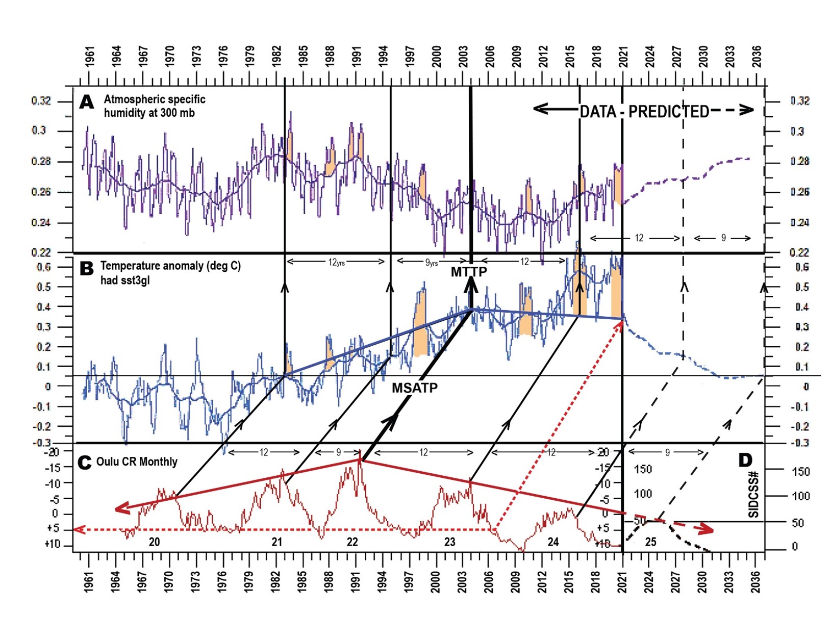
I was responding to your quote, in which you stated that UAH “shows that there has been no net global warming for the last 18 years”.
That’s completely wrong. UAH shows statistically significant warming over the past 18 years.
I said The correlative UAH 6.0 satellite TLT anomaly at the MTTP at 2003/12 was + 0.26C. The temperature anomaly at 2021/11 was + 0.08 C. (34)
Check the data at Ref (34)
https://www.nsstc.uah.edu/data/msu/v6.0/tlt/uahncdc_lt_6.0.txt accessed 12/02/2021
“I said The correlative UAH 6.0 satellite TLT anomaly at the MTTP at 2003/12 was + 0.26C. The temperature anomaly at 2021/11 was + 0.08 C”
So what?
In July 2004 it was -0.36C and in Feb 2020 it was 0.59C ( delta of 0.95 ).
Not only does the Sun not cause any more that 0.1% of a differential in TSI over it’s entire ~ 11 year cycle but it also doesn’t act that quickly ( ~ 7 – 10 months).
How about you have a chat with Leif Svalgaard to confirm that.
Both yours and my examples of NV with the data are an irrelevant and meaningless metric, as the up/downs in the data series (as in any other satellite series …. Less so in surface datasets as sat radiometers are sensitive to WV which is the main driver of NV “measured” by UAH V6 TLT – and is caused by the ENSO cycle).
Try drawing a Mean line of least squares eh.
A quick eyeball of it gives me a rise of 0.25C in that time (mid 2003 to now).
Or ~ +0.2C/decade.
Mr Page says it is not a good idea to start a trend on an el Nino peak. As the head posting clearly explains, the trend begins at the furthest point in the past from which the global mean surface or lower-troposphere temperature trend is zero or less. As the two graphs in the head posting clearly show, neither graph starts at an el Nino peak. Furthermore, the method of calculating least-squares linear-regression trends considers every data point, not just the start point and the end point.
If you ignore the El Nino periods of 2015-2017 and 2019 then the preponderance of annual temperatures since 2004 are less than the temperature for 2004. Look at the charts from UAH not NASA charts.
How do you handle the La Nina periods?
The El Nino’s are coloured yellow in Fig 5 above. They are short term deviations from the general trend.
The same way if you can identify them. They are not as prominent as El Nino.
I ignored all El Nino and La Nina periods using the ONI to identify them. The average ONI of the remaining 248 months was 0.00 C. The warming trend of these months is +0.133 ± 0.008 C/decade vs the +0.135 ± 0.006 C/decade with all 513 months available. There is no statistical difference between the warming as-is and the warming trend sans ENSO.
By studying the chart or graph of world-wide temperatures starting in the 1880’s.
I love Monckton. Funny and scientifically accurate. I can’t remember when I got redpilled on climate science, but I do remember being struck with the obvious irrefutability of the Monckton math on ECS.
Adding not-unreasonable uncertainty limits of ±3.4°C to the UAH temperature time series increases the standard deviation of the slope of the line regression fit from 0.6 mK/yr to 8.5 mK/yr, which is more than half the magnitude of the slope itself. Considering that the line fit can lie anywhere within the confidence interval, it is not unreasonable to say the entire 41-year time series has been a pause.
Monte Carlo
” … not-unreasonable uncertainty limits of ±3.4°C… ”
Hmmmh.
Science has not anything to do with ‘(un)reasonable’.
I await your scientific calculation of this uncertainty according to the mechanism which you should have in mind, together with an exact hint on a scientific paper showing the theory this mechanism is verifiably based on.
https://wattsupwiththat.com/2021/12/02/uah-global-temperature-update-for-november-2021-0-08-deg-c/#comment-3401727
With references.
Thank you, this is the very first time I see a comment of yours avoiding any polemic.
I will go into that stuff when I have some idle time for, in the hope to find what I’m looking for.
*
My problem with the very certainly possible uncertainties associated with temperature time series
is e.g. this:
How is it possible that these series show such a convergence (of course only in anomaly form, due to partly different absolute values) ?
Uncertainty is not error, instead it is a quantification of the reliability of a numeric measurement result.
Replot these as actual temperatures, without the baseline subtractions and without any smoothing.
And before I start reading during the week-end, feel free to feed me meanwhile with the information I primarily asked for:
” I await your scientific calculation of this uncertainty according to the mechanism which you should have in mind, together with an exact hint on a scientific paper showing the theory this mechanism is verifiably based on. ”
Because all these links you provided are indeed sources for uncertainties, but they tell me nothing about how you derived ‘±3.4°C‘ out of all them. nor did you mention the mathematical background you used to to the job.
Start reading its all in there.
On the contrary! Any good researcher will peruse their calculations and conclusions for reasonableness. It was much more common when people used slide rules and routinely had to estimate where to place the decimal point in the three digits read off the slide rule. Order of magnitude is just one kind of error that can be made using a computer if one doesn’t at least do a mental calculation of what the approximate answer should be. Other kinds of errors are forgetting to divide by a critical number like 2, or forgetting to multiply by Pi. Someone who doesn’t verify reasonableness is just being lazy, or perhaps received an inferior education.
carlo, monte
“Adding not-unreasonable uncertainty limits of ±3.4°C to the UAH temperature time series increases the standard deviation of the slope of the line regression fit from 0.6 mK/yr to 8.5 mK/yr”
I asked before, what maths are you using to calculate the standard deviation of the slope?
x = X – <X>
y = Y – <Y>
sum_x^2 = Σxx
sum_y^2 = Σyy
sum_xy = Σxy
sum_d_yx^2 = sum_y^2 – (sum_xy)^2 / sum_x^2
s_yx = sqrt{ sum_d_yx^2 / (n-2) }
s_b = s_yx / sqrt{ sum_x^2 }
Where in that string of equations does the uncertainty of the measurements get factored in?
Strictly speaking, the propagation of error should be accounted for with every mathematical operation defined in the equation’s variables. Unfortunately, it rarely is. Most mathematicians and statisticians tend to treat statistical equations as though they were working with exact numbers. Sometimes they are. However, not always.
Deleted this comment, as I made a mistake.
I’m not sure about the logic of applying uncertainty propagation to equations that are already trying to determine the uncertainty. But I’d like to see you give a worked example.
Instead of whacking through all the weeds, how about a thought experiment?
Why should any equation be handled any differently than another using the same measurements?
Every measurement has a limit to the precision with which it can be measured. There have long been Rules of Thumb that require that in a sequence of multiplications (or the inverse, division), one is not justified in retaining more significant figures than in the factor with the least number of significant figures. That is universal, no matter what is being calculated!
In sampling a population, random errors of measurement will give a distribution that clusters around a central value. One should take into consideration the precision of the measurements, which limit the number of significant figures of the average, to the precision of the least precise measurement. Dealing with integers, which are exact, there is no problem. However, dealing with real-world measurements, there are always issues of precision.
As Monte illustrates above, in calculating the SD, one uses the summations of the products of measured variables. A rigorous treatment requires adding the uncertainties, which is at least as large as half the next digit position. In the case of noisy data, there will be an additional random error, which the variance allows us to estimate. Once the standard deviation is calculated, it, or the estimate obtained from the Empirical Rule, using the range, should be applied to all subsequent statistical derivations such as the standard error. This uncertainty is typically larger than the error imposed by precision, and can be quite large for non-stationary data, where the mean and standard deviation change over time.
Good description.
“This uncertainty is typically larger than the error imposed by precision, and can be quite large for non-stationary data, where the mean and standard deviation change over time.”
Per provided demo, w.r.t. physically/statistically significant time periods – the only ones that should be seriously considered – including the errors correctly aggregated from station data and spatial interpolation, into monthly or yearly temperature or sea level estimates, changes the statistical durability of the resulting standard errors of the trends, hardly at all.
Remember. “Use your words”? Use your numbers Clyde. Correctly. Not your prejudged intuition…..
Another blob(TM) Word Salad.
“including the errors correctly aggregated from station data and spatial interpolation, into monthly or yearly temperature or sea level estimates, changes the statistical durability of the resulting standard errors of the trends, hardly at all.”
You don’t specify how they can be correctly aggregated so how do you know they don’t affect the statistical durability of the standard errors of the trends?
Temps in the NH are going up while at the same time they are going down in the SH. How are those correctly aggregated on a monthly basis without affecting the temperature trend of the combination?
“You don’t specify how they can be correctly aggregated so how do you know they don’t affect the statistical durability of the standard errors of the trends?”
The expected value data points are from a spatial interpolation of the individual stations. To distribute those points, first the known error distributions of the individual measurements are accounted for. Then, the standard deviation of the spatial interpolation. These are then combined – in a manner probably similar to mine – to arrive at a distributed value for each data point. This is what you see in the gistemp evaluation I performed. From that, any trending can be done that includes both the least squares variance and the sum of the variances from the data point distributions. When combined, you figure out the standard error of the trend, with all things considered.
“Temps in the NH are going up while at the same time they are going down in the SH. How are those correctly aggregated on a monthly basis without affecting the temperature trend of the combination?”
Probably the way it’s been done for decades…
Spatial interpolation depends on the assumption of homogeneity. The correlation coefficient for stations more than 50 miles apart is only 0.8. Other factors such as elevation and terrain lower the factor even more. In other words, most people wouldn’t consider the correlation to be very high.
How do you account for something you don’t know? Temperature measurements by field stations have uncertainties that cannot be quantified.
Garbage. This isn’t even a complete sentence.
Again, more garbage. What is a “distributed value” for each data point? Especially when the correlation factor is so low?
In other words you infilled data to points using uncorrelated data. And you think that gave you a valid answer?
In other words the fact that the base data represents a multi-modal distribution is ignored just like the uncertainties associated with each temperature measurement!
It is totally dismaying how far science has fallen.
You his a nerve in the blob, he gave you a downvote.
All the way down to blatant pseudoscience. They have absolutely no reasoning skills.
“Spatial interpolation depends on the assumption of homogeneity. The correlation coefficient for stations more than 50 miles apart is only 0.8.”
Yes, temperatures change at different rates in different microclimates. What does that have to do with anything being discussed here. In particular, why can’t you do spatial interpolation with those differences? Please provide a link to any tech literature discussing this non problem.
“How do you account for something you don’t know? Temperature measurements by field stations have uncertainties that cannot be quantified.”
Simply not the fact. Although older temperature gathering methods were both less precise and accurate (not to mention less convenient) than newer ones, the precision and accuracy of every one of them was known at the time and is now known even better.
“Again, more garbage. What is a “distributed value” for each data point? Especially when the correlation factor is so low?”
One paragraph, 2 willful misunderstandings. The “distributed value” for a given temperature measurement method is the range of it’s possible actual values, and the distribution of it’s diminishing chance of occurrence, away from it’s mean. It is known. OTOH, your “correlation” is between expected values from one station to the next. From one time to another, one might rise, one might fall. Means nada to the temporal spatial interpolations. You don’t seem to have a real understanding of any of this.
“In other words you infilled data to points using uncorrelated data. And you think that gave you a valid answer?
Again, this is something you’ve heard, but have no actual understanding of. Why would you need to “correlate” these values, in spatial interpolation? Again, please provide any literature requiring this. Perhaps you’re confusing correlatable error distributions for a given data gathering method, with changes over time between stations. If so, please note, for that any correlations between temperature measurements taken during one period, and aggregated into a regional/global average for that period, you are limited by 2 types. No correlation, or a positive correlation. Negatively correlating such error bands would make no physical sense. That leaves you the analysis I did, which didn’t correlate individual GAT possible ranges, and one that would have. Guess which would change the standard error of the resulting trend by more.
“In other words the fact that the base data represents a multi-modal distribution is ignored just like the uncertainties associated with each temperature measurement!”
Plz expand on these invented “multi modal distributions” But even given them, they could still be evaluated. In fact, any combo of continuous (or even step function) distributions can not only be properly evaluated, but (more bad news for you), the resultant evaluated parameter will tend towards a normal distribution, per Engineering Statistics 101.
Another load of blob bloviation.
Well done blob!
Temperature is a time function. Daily, monthly, and annually. That’s what the mileage is a measure of. The actual function that needs to be evaluated is f(x) = sin(t) + sin(t + φ). When you analyze this for correlation between stations a “t” and at (t+φ) the correlation is cos(φ). As a first estimation “φ” equates to about 50 miles. I’ve never actually tried to evaluate it any more accurately. And that mileage can be either latitude or latitude.
If you are going to infill the temp at one location to another location you *must* make sure that the correlation between the two locations is pretty high.
You just got the technical details. If you can’t figure it out from there then you have no business trying to speak to the subject.
I can give you other factors in φ. Terrain is one. Is one station on one side of a mountain range and the other station on the other side? Elevation is another. Temps at the top of Pikes Peak shouldn’t be infilled to Denver or Colorado Springs because of the elevation difference.
There is at least one paper here on WUWT that addresses this. It was several years ago. Ask Anthony if he can point you to it.
Nope. It has nothing to so with error but solely with correlation based on several factors.
Again, it has nothing to do with error bands. How do you average Northern Hemisphere temps with Southern Hemisphere temps. They are certainly either negatively correlated or uncorrelated. In fact they represent a multi-nodal distribution. Where in any climate study have you seen where the researchers use multi-nodal techniques?
Nope. The precision may have been known but not the accuracy. Every measurement site has different reflectivity material below it. E.g. green grass, dirt, brown grass. asphalt, etc. Who knows what these different materials do to the uncertainty – a measure of possible accuracy. Hubbard even says that any correction of older measurement stations must be done on a station-by-station basis because of the varying instrument drifts, varying environment, varying shield types, etc.
Hubbard even found that this applies to newer stations. And Hubbard didn’t even allow for environmental uncertainty such as failing fans in a shield, air intakes blocked by wasp nests, etc. Nor did he attempt to measure urban heat impacts.
Unfreaking believable! I have tracked temperatures on the north side and south side of the Kansas River valley here in Kansas since 2002. They are almost never the same and are only 25 miles apart. This could be because of uncertainty in the measuring instruments or because of environmental effects (elevation, humidity, pressure, etc).
Why would you possibly think that infilling the temp from one of these stations to the other would be justified?
No, actual temps are *NOT* known. See the paragraphs above. Means change because of weather, distance, elevation, humidity, etc. These are *not* common among stations, even ones close in distance.
I get the feeling that you are mostly familiar with time-invariant functions.
Pick a date, assume July 1. Avg temp Kansas City is about 75F (66F to 90F). Average temp in Buenos Aires is about 55F (49F to 60f). That’s a bi-modal distribution. Map those and you will get a double-hump distribution. As you move in latitude you will find lots of humps – i.e. multi-model.
I am at a loss as to what you mean by “properly evaluated”. What kind of evaluation are you talking about? What do you think the mean and standard deviation of a double-hump distribution like one put together from KC and BA data will be? What will those actually tell you?
“the resultant evaluated parameter will tend towards a normal distribution, per Engineering Statistics 101.”
What evaluated parameter? How does a double-hump distribution all of a sudden become normal? Daily temps pretty much follow a sine wave. Do you have a clue as to what the probability distribution of a sine wave is?
The inversion layer can cause 10-20F variations within the Denver metro area!
In the data, of course.
But if the uncertainty is already present in the data, how does changing the uncertainty affect the confidence interval?
I’m sure your Excel Ouija board can answer the question.
You’re the expert here, you should easily be able to sort it out.
Haven’t used Excel in a long time. I’m absolutely not an expert, which is why I keep asking you to explain your methods. I’m quite prepared to believe there an advanced system for including measurement uncertainties in the confidence interval of a linear regression. But your inability to provide a straight answer makes me doubt it.
All I’m trying to get at here is how adding uncertainty limits of ± 3.4°C to the time series, increased the confidence interval of the linear regression by a factor of 10. I assume you have some technique to justify that claim, and would like to know what it is.
You’re the smart expert here on statistics and uncertainty, Shirley you can figure it out.
There is no function directly in excel or equivalent freeware to do this. I’m, stuck on a train for the next 4 hours, so I’ll try and work up an example of how to calc this, and check it.
As an example, download 1980 – present gistemp temp data, into excel, freecalc, or other freeware that uses excel functions (most).
You should get a trend of 0.017323 deg/year, with a standard error of that trend of 0.001233 deg/year.
You should get 0.093395 deg. So, the variance is 0.008723 deg^2.
We are using 41 years of data, so the sum of the variances is 0.008723 deg^2 * 41 years, or 0.357629 deg^2 * year
You should get 0.006638 deg^2 * year
So, the total of the 2 sums of variances should be 0.364266 deg^2 * year.
Wish I could download my workbook….
Visually, where will a random sample of one distributed data point land? Your first random sample is of where it would land from the standard deviation of it’s distance from it’s least squares location. But then, from that point, you must then change it’s position again, according to a random sample of the (provided) standard deviation of that data point. So, 2 standard deviations, 2 variations, and the variance of the sum is equal to the sum of the variance. Sub “square of the standard deviations” for “variances” and there you are.
A units mistake. deg2/year should be deg2/year^2. But the units all clear out in the later maths, so no wrong numbers.
Thanks for all this work. I’m going to try to work through it when I have time, probably using R rather than a spread sheet.
Oh dear. I’ll use my workplace – AMTRAK coach – as an excuse, but it won’t wash. This is embarrassing.
“We are using 41 years of data, so the sum of the variances is 0.008723 deg^2 * 41 years, or 0.357629 deg^2 * year”
“You should get 0.006638 deg^2 * year.”
No matter what Pat Frank believes, adding temperature variances over a period of years does not change their units. The correct units for this are deg^2. STILL washes away in the later maths though, so the numbers are still ok.
You’re an idiot, blob, just in case you don’t realize this obvious fact.
Don’t worry, I was going to ask if I was doing something wrong as I kept getting the 0.006638 figure.
One thing I had noticed is that the temperature data is the same for the last 3 years. I assume this just means they haven’t updated it yet.
Good eye. You’re probably correct. If you leave out the last 3 years, the standard error of the trend changes by ~0.9% instead of ~1.0% by including the standard deviations of the individual data points.
Point is, evaluate any physically/statistically significant temp or sea level sets with direct or calculable standard deviation data, and you will see that those “error bands” don’t qualitatively change the statistical durability of those trends a bit. Would be nice to be able to completely disarm the Dr. Evil conspiracy theorists with a drill down of the error analyses for every measurement method, everywhere, for the last 150 years. But:
Next, helping those Bizarro Worlders who think that more data = more error, to snap out of it…
The uncertainty of the measurements is not included in Carlo,Monte’s work up. The sum of variance he uses is calculated from taking the diff between each actual value and it’s calculated value. But you can easily calculate the other sum of variance by using the variance of the error of each value, and adding them up. You then total both sources of sum of variance and complete the standard error of the trend calculation using that.
The problem for this all purpose excuse for AGW denial is that, even given the greater error bands from older temperature measurement methods, for statistically/physically significant time periods, temperature measurement error change the standard error of the temperature trends hardly at all. This is why commenters here whine about how bad the old methods were, to no end, but don’t do the arithmetic to actually show how (un)important those measurement error really are w.r.t. the trends under discussion.
Samo samo with sea level station data evaluation….
Of course it is, blob is just resorting to lies (again).
“Of course it is, blob is just resorting to lies (again).”
No, it is not. You have the (correct) progression of terms that lead up to a calculation of the standard error of a trend. But using only deterministic data points. Not a thing wrong with that, especially considering the insignificant practical effect of including the distributions of each data point in temperature and sea level trends over physically/statistically significant time periods. I.e., the bogus point that Clyde Spencer et. al. make, with out ever actually evaluating any real data, about every other post….
blob resorts to posting technobabble.
Thanks, I think I see what you mean, but I’m not sure about adding both variances together. I would assume that any variance from the uncertainty was already in the variance of the measured values.
One other question. Do you know what the sum_d_yx^2 part of his equation is doing? All the online sources just use sum_y^2 in the final equation. I’m assuming this is part of a more advanced method, rather than just a mistake.
“Thanks, I think I see what you mean, but I’m not sure about adding both variances together. I would assume that any variance from the uncertainty was already in the variance of the measured values.”
It is correct. Download a sea level station with distributed data. Then, using either excel or a freeware like freecalc, and step by step, solve for the standard error of the trend, first using just the data expected values, and then finding the sum of variances that linest uses, the sum of variances supplied from the standard deviations of the sea level data, adding them, and finding a parameter linest standard error*((total sums of variance)/linest sum of variance using only expected values)^0.5. Then, using the norminv and rand functions, calculate a couple thousand realizations of the data and, using linest, find the standard errors of the trends for all of them. Find the average of all of those standard errors, and you will find that it converges perfectly upon your earlier answer. To my point, you will see how little including those standard deviations changed the standard error of your trend. Same with GAT data.
“One other question. Do you know what the sum_d_yx^2 part of his equation is doing? “
Got me there. I spaced on that, and don’t know either. The equation looked ok generally, and I was trying to find common ground. He took it from a book and either typo,d or otherwise mistransferred it. He didn’t really know what he was typing….
blob hath declared TRVTH.
The UAH TLT 1991-2020 baseline for November is 263.406 K as computed from here. Do you really think the November 2021 value could be as 259.922 K or as high as 266.722 K?
Great! You’ve shown (again) for all to see you have no clues about uncertainty.
As usual, the Honorable Third Viscount proudly presents his good old trick, which is to calculate the linear estimate for a period in a time series starting with the highest value in that series.
Well done! The estimate hardly could be positive.
Linear trends for UAH 6.0 LT, in °C / decade
In such a context, going back in the series as long as your estimate is near 0: that is really a bit brazen; and above all, it tells nothing.
La vie est simple, profitons-en!
Ha! A downvote! More of them, please! I love them.
I have often found that a down vote here is often a up vote for truth.
A contrary of truth is for example falseness.
Can you show me where you find it in my comment?
Binindon,
I did not give you any vote (not up and not down) because that would not refute your fallacious twaddle.
You provide cherry-picked data based on choice of starting point whereas Viscount Monckton starts at now – whenever now is – and analyses data in the time series back from that point whatever it is.
a)
The “start” of the assessed pause is now
and
(b) the length of the pause is the time back from now until a trend is observed to exist at 90% confidence within the assessed time series of global average temperature (GAT).
The resulting “pause” is the length of time before now when there was no discernible trend according to the assessed time series of GAT.
90% confidence is used because that is normal for ‘climate so-called science’ but 95% confidence is usual for most real science.
Richard
PS The large number of anonymous trolls posting misinformation in this thread suggests ‘troll central’ is alarmed by the subject but lacks minions with ability.
I am in complete agreement with this postscript.
But do you agree with the rest of his comment?
Where are you getting 90% confidence for the trend of -0.005C in UAH since Jan 2015?
The 95% confidence for it (which, despite what you say, is the standard confidence threshold in climate science) is ±0.677!
Richard Courtney is correct: the trolls are largely pseudonymous; they are numerous; and they are strikingly scientifically illiterate. But they are handsomely paid by the various Communist front groups masquerading as “environmentalist” organizations, so they think it worthwhile to post their drivel here. It is of course valuable to the intelligence community to know which arguments the climate Communists fear. The whining of the pseudonymous climate Communists here is of particular value in revealing how terrified the Party is that a prolongation of the present Pause will bring the global-warming nonsense to an end.
Monckton:
“Richard Courtney is correct: the trolls are largely pseudonymous; they are numerous; and they are strikingly scientifically illiterate.”
Says he with his qualifications in “Journalism” and “The Classics”.
What hypocrisy.
Well I’m not anonymous and am a retired UKMO Meteorologist – I have forgotten more meteorology than you know.
And again the group-identify ideation.
I’m not a “Communist”, nor even a “Socialist’.
It is possible to understand the science on it’s own merit.
Which is why there are no credible experts who don’t.
That you identify with your political peers on the right does not make those that disagree with you “the left”, especially not in the scientific field that you have no qualifications in (yes, yes we know you have “colleagues” who are … and are anonymous BTW – more hypocrisy on your part).
And to turn it into an ideological struggle is just another Monckton MO that reeks with hypocrisy.
Anthony Banton,
Please
1. define “credible” when you say ” credible experts”
and
2. explain how your definition would apply to (a) A Einstein at the time when he published his seminal papers on relativity and (b) W and O Wright when they published their seminal work on aviation.
It seems you would benefit from understanding the importance of nullius in verba.
Richard
“Please
1. define “credible” when you say ” credible experts””
All of the thousands of climate (and other Earth) scientists that contribute to the IPCC ARs.
Vs the tiny minority of those often featured here.
”2. explain how your definition would apply to (a) A Einstein at the time when he published his seminal papers on relativity and (b) W and O Wright when they published their seminal work on aviation.”
Dear oh dear, that old trope.
Mr Einstein published his papers on Relativity in between 1905 and 1915. Well over 100 years ago.
He hardly had anyone else thinking along those lines now did he. He was a maverick genius.
How can anyone with a modicum a common-sense think the two are equatable, with there being with there being thousands of scientists looking into climate science.
Again the Wright brothers came at the end of the 19th century.
Again pioneers and not one on many thousands working in the field.
In short an hilarious false comparison.
And what did you say about nullius in verba?
As I’ve just outlined – thousands of scientists vs a few ideologically motivated, err, “sceptics.”
Comes a point when there just ain’t any reasonable option.
Unless your peer-group and ideologically motivated cognitive dissonance takes over said common sense.
Alternative:
Chaos where we would believe no one because we (someone/anyone) don’t like what it is they are saying.
Anthony Bantonn
In answer to my asking
“Please
1. define “credible” when you say ” credible experts””
You have replied
“All of the thousands of climate (and other Earth) scientists that contribute to the IPCC ARs.
Vs the tiny minority of those often featured here”
That is daft. At very least your use of “Vs” is ridiculous because, for example, I am in both groups and I assure you that I do not oppose myself.
I made no “comparison”. I asked how a theoretician, A Einstein, and some experimentalists, the Wright brothers. fitted your definition of “credible experts”. You say they were not “credible experts” because they worked long ago. Well, of course, that is correct according to your daft definition because the IPCC did not exist when they were working.
In reality, it is you and your daft definition of “credible” which lack credibility. The credibility of A Einstein is demonstrated by the development of much of modern physics and the credibility of the Wright brothers by e.g. the existence of Airbus Industries. While the lack of expertise of those you support is demonstrated by the stasis in ‘climate so-called science” which has existed for the last four decades (e.g. there has been no reduction to the range of assumed equilibrium climate sensitivity, ECS, for 40 years).
Ideology is irrelevant to real science. Clearly, it motivates you.
I repeat,
It seems you would benefit from understanding the importance of nullius in verba.
Richard
“I repeat,
It seems you would benefit from understanding the importance of nullius in verba.”
Richard — Of course it makes no sense to you !!!!!
In no way do I expect to overturn your down-the-rabbit-hole thinking.
And that’s OK because I repeat as well….
And state that at some stage common-sense has to prevail in order to act on any finding whether scientific or otherwise, given a consensus that it is necessary.
Thousands of Climate and Earth scientists have and politicians do.
To allude to Einstein and the Wright brothers as example of mavericks as though someone is going to come along and “disprove” the GHE as pertaining to mankind burning fossil carbon is bizarre.
How long to you propose to wait for this genius to upturn over 150 years of thermodynamical science before your ideological bias and cognitive dissonance allows that you may be wrong?
Anthony Banton,
Your witless and childish insults are not a rational alternative to serious discussion and, importantly, they fail as a smokescreen intended to hide your total inability to answer my complete demolition of your silly assertions.
The GHE has existed since before the human race came into being.
I will agree my understanding of ‘climate so-called science’ is wrong when there is some (n.b any) empirical evidence for discernible anthropogenic (i.e. human induced) global warming (AGW). I know this is a mystery to you, but it is the position adopted by all real scientists.
I again ask you to learn about nullius in verba because it is a motto that has been the foundation of real science since the Reformation: if you can grasp the concept it represents then real science will cease to be a mystery to you.
Richard
Both of your examples started small and grew. AGW denialism is going the opposite way.
Mr Banton, a Communist, who, like nearly all Communists, denies that he is a Communist, as usual has nothing scientific to offer. But at least he now publishes here under his own name, after being outed by me once I had had him traced.
As far as I am aware, Mr Banton’s record of publication in the journals of climate science and economics is precisely zero, whereas I have had more papers published than some Professors before they get tenure. Only a Communist would believe that it is only once one has had appropriate and certified Socialist training in a given topic that one can be considered competent in it.
In the West that Mr Banton so viscerally hates, we enjoy four great freedoms: of election, of religion, of markets and of speech, thought and publication. I choose to exercise those freedoms. Mr Banton chooses to whine about them. Which of the two is more attractive?
Oh dear, Brench. I thought I was on the Guardian “climate crisis” blogsite for a moment. You know, Graham Readfearn or Oliver Milman or Damian Carrington?
Give it a rest.
Don’t whine.
Glad to oblige!
The handsomely-paid climate Communist “bindidon” makes the elementary scientific error of assuming that I search for spikes in global temperature and start my Pauses therefrom. As I have explained before, and will now explain again, the Pauses are simply the longest periods up to the present for which a given dataset shows a least-squares linear-regression trend no greater than zero. In fact, there have been several sharp spikes in global temperature, but those spikes are caused by naturally-occurring el Nino events. During the previous Pause, the paid climate Communists went on and on whining about the presence of el Nino spikes at or near the beginning of the Pause, even though a subsequent spike of near-equal magnitude had the effect of canceling the influence of the first spike. The truth is that global warming may well be largely an artefact of the celestial mechanics that are a significant cause of the crustal deformations that drive el Ninos.
The reactions are a demonstration that any threat to the warming ideology is an act of heresy to the Church of Climastrology.
Oh I get upgraded to a communist!
Wonderful.
Tells everything about what is in your mind, Third Viscount of Brenchley…
You are such an aggressive person!
One cannot be aggressive to paid climate-Communist trolls when they furtively post here under pseudonyms. If you post under a pseudonym, expect to be called out as the paid enemy of freedom that you are, and don’t whine about it.
Nonsense. He calculates his trend using negative time which starts now. You cannot even get the sign of the determining factor in the calculation straight in your criticism, which makes it utterly useless as an argument on your part.
“There is no need to do anything at all about global warming except to enjoy it.”
Meanwhile, Auckland Mayor, Phil Goff, has just introduced a climate tax on the ratepayers.
Our leaders outright refuse to see the mountains of evidence that show there is no climate crisis.
How do we make it stop when evidence is irrelevant?
Oh, I think there’s a wee typo in this word “lackwit”. I think you got the first two letters wrong.
LM says”…minuscule feedback response to direct warming forced by greenhouse gases.”
I have never seen an experiment or other evidence that there is any forced warming from greenhouse gases. If you have one please share.
Tyndall (1851).
So Tyndall measured the warming from ghgs? I don’t think so.
You sound like a warmist, Brench. You could have cited Svante Arrhenius or Eunice Foote but would still be wrong.
The furtively pseudonymous “leitmotif” seems unaware of the details of the experiments at the Royal Institution 170 years ago. Tyndall indeed demonstrated that CO2 has a warming effect, though it is not easy to derive the magnitude of the expected warming from such experiments.
And to cite scientific authorities is not wrong (though the scientific authorities themselves may be wrong).
Gee, Christopher, why don’t you tell us what you really think?
No malice intended.
And no offence taken. The livery company to which I belong in the City of London has the following song:
“Oh, give us your plain-dealing fellows,
Who never from honesty shrink,
Not thinking of all they shall tell us,
But telling us all that they think.
I speak plainly. I was brought up to do that.
Which livery company is that, Christopher?
Speaking plainly is not appreciated in bureaucracies. Its one of the reasons I quit the U.S. government after eleven years at a fairly high level.
Unfortunately the alarmists don’t care much for logic and scientific proof that disagrees with their dogma. They want climate justice, which imo means redistribution of wealth. In other words it’s nothing to do with climate. When they have hounded the poor into even more “green” poverty that will just confirm in their perverse minds the climate injustice!