Guest essay by Bevan Dockery
Here is 38 years of empirical data clearly showing a relationship between the satellite temperature and the rate of change of atmospheric CO2 concentration at the Mauna Loa Observatory.

Figure 1. Mauna Loa Observatory
Figure 1 shows the monthly lower tropospheric satellite temperature for the Tropics-Land component in blue and the annual change in CO2 concentration in red. The obvious correlation between the two raises the possibility that there may be some common causal factor whereby the temperature drives the rate of change of CO2 concentration. It is not possible for the rate of change of CO2 to cause the temperature level as a time rate of change does not define a base. For example a rate of 2 ppm per annum could be from 0 to 2 ppm in 12 months, 456 to 458 ppm in 12 months or any other pair of numbers that differ by 2.
Note that the satellite temperature data is supplied as a residual after removal of the estimated seasonal variation. This makes it comparable to the annual rate of change of CO2 concentration as taking the annual rate eliminates the seasonal variation.
Calculation of the Ordinary Linear Regression between the two time series gave a correlation coefficient of 0.65 from the 448 monthly data pairs. Detrending of the time series in order to determine the statistical significance gave a correlation coefficient of 0.56 with 446 degrees of freedom. However the Durbin-Watson test of the time series gave a value of 1.08 indicating positive autocorrelation which means that Ordinary Linear Regression is inapplicable. The autocorrelation was estimated to be 0.53. When applied to the transformed time series, that is, applying a First Order Autoregressive Model, it resulted in a correlation coefficient of 0.25 with 445 degrees of freedom and a t statistic of 5.38, implying an infinitesimal probability that the coefficient is equal to zero from a two-sided t-test.
Applying a First Order Autoregressive Model to the Tropics-Ocean component of the satellite temperature compared to the annual change in CO2 concentration gave a correlation coefficient of 0.14 with 445 degrees of freedom and a t statistic of 3.06, implying a probability of 0.2% that the coefficient is equal to zero from a two-sided t-test.
It follows that this synthesis of empirical data conclusively reveals that CO2 has not caused temperature change over the past 38 years but that the rate of change in CO2 concentration may have been influenced to a statistically significant degree by the temperature level. Note that it is not possible for a rise in CO2 concentration to cause the temperature to increase and for the temperature level to control the rate of change of CO2 concentration as this would mean that there was a positive feedback loop causing both CO2 concentration and temperature to rise continuously and the oceans would have evaporated long ago.
Support for this thesis is seen in a statistical analysis of the monthly CO2 concentration with respect to the lower tropospheric temperature for Macquarie Island in the Southern Ocean at Latitude 54̊ 29ʹ South, Longitude 158̊ 58ʹ East. Applying a First Order Autoregressive Model to the various components of the temperature, Global, Southern Hemisphere, Tropics, and Southern Extension and their Land and Ocean components gave correlation coefficients ranging from a minimum of 0.01 for 284 degrees of freedom, t statistic 0.15, probability of zero correlation 88% for the Southern Hemisphere zone, 90̊S to 0̊, to a maximum of 0.55, 284 deg. of free., t statistic 10.97, infinitesimal probability of zero correlation for the Tropics temperature zone, 20̊S to 20̊N.
This explains the well known fact that CO2 change lags temperature change over a large time range. Ice core data has revealed that the cycle of ice ages and interglacial warm periods shows CO2 change lagging temperature change by several centuries to more than a millennium while modern CO2 and temperature data shows lags of 9 to 12 months, Humlum et el., 2013 [1]. Cross correlation of annual changes in each of CO2 concentration at Mauna Loa and satellite lower tropospheric Tropics – Land temperature showed that CO2 change lagged temperature change by 5 months. As temperature controls the rate of change of CO2 concentration, local maxima in the CO2 rate must correspond to temperature maxima which, mathematically, must occur after the maxima in the rate of change of temperature. Likewise the CO2 concentration maxima must post-date the maxima in the CO2 rate and thus post-date the corresponding temperature maxima. Put simply, CO2 does not cause global warming.
The CO2 concentration data for the Mauna Loa Observatory is freely available from the Scripps Institute via the Web page:
http://scrippsco2.ucsd.edu/data/atmospheric_co2
The satellite temperature data for the Tropics zone is freely available from the University of Alabama, Huntsville, Dr Roy Spencer’s Web site at:
http://www.nsstc.uah.edu/data/msu/v6.0beta/tlt/uahncdc_lt_6.0beta5.txt
The CO2 concentration data for Macquarie Island is available at: http://ds.data.jma.go.jp/gmd/wdcgg/pub/data/current/co2/monthly/mqa554s00.csiro.as.fl.co2.nl.mo.dat
The above conclusion is totally at odds with the statements from the United Nations climate body, the Intergovernmental Panel on Climate Change. The Policymakers Summary from Climate Change, The IPCC Scientific Assessment, 1990, being the, then, final Report of Working Group 1 of the IPCC, opened with the statement, page XI:
“EXECUTIVE SUMMARY
We are certain of the following:
• there is a natural greenhouse effect which already keeps the Earth warmer than it would otherwise be
• emissions resulting from human activities are substantially increasing the atmospheric concentrations of the greenhouse gases carbon dioxide, methane, chlorofluorocarbons (CFCs) and nitrous oxide. These increases will enhance the greenhouse effect, resulting on average in an additional warming of the Earth’s surface. The main greenhouse gas, water vapour, will increase in response to global warming and further enhance it.” – end quote.
After decades of research into the relationship between the atmospheric CO2 concentration and temperature, the latest, Fifth Assessment Report, 2015, of the IPCC, the Synthesis Report, Summary for Policymakers, page 8, made the claim:
“SPM 2.1 Key drivers of future climate
Cumulative emissions of CO2 largely determine global mean surface warming by the late 21st century and beyond. …….” – end quote.
Here again is 38 years of empirical data, this time showing a distinct lack of a relationship between the satellite temperature and the atmospheric CO2 concentration.
Figure 2. Mauna Loa Observatory

Figure 2 shows the monthly lower tropospheric satellite temperature for the Tropics-Land component in blue and the monthly CO2 concentration in red after removal of the seasonal variation so as to match the residual temperature series. The clear and obvious difference between the two raises the possibility that there may be no common causal factor whereby the CO2 concentration drives the temperature as claimed by the IPCC.
Calculation of the Ordinary Linear Regression between the two time series gave a correlation coefficient of 0.49 from the 454 monthly data pairs. This is a measure of the relationship between the background linear trend of each of the time series as shown by the almost identical correlation between the temperature and the time of 0.50. The correlation between the CO2 concentration and the time was 1.00, that is, the CO2 concentration time series was practically a linear trend as is the time. Any pair of linear trends, no matter what their source, will have a high correlation coefficient of about 1.0 which is necessarily of no causal significance as every time series has a background linear trend with respect to time.
Detrending of the time series in order to determine the statistical significance gave a correlation coefficient of 0.0015 with 452 degrees of freedom. However, the Durbin-Watson test of the time series gave a value of 2.40 which indicates negative autocorrelation. The autocorrelation was estimated to be -0.79. Applying a First Order Autoregressive Model to the two transformed time series resulted in a correlation coefficient of 0.002 with 451 degrees of freedom and a t statistic of 0.047 implying a probability of 96% that the correlation coefficient is equal to zero from the two-sided t-test.
Once again the Macquarie Island data support this result. The Island is in the Southern Extension zone of the satellite lower tropospheric temperature data, latitudes 90̊ South to 20̊ South. Analysis of the temperature data for the complete zone and its Land and Ocean components with respect to the CO2 concentration showed that there was positive autoregression in each case requiring a First Order Autoregressive Model to be applied. The result for the whole zone was a correlation coefficient of -0.06, 296 deg. of free, t statistic -0.98, probability of zero correlation 33%. For the Land component, the correlation coefficient was -0.02, 296 deg. of free, t statistic -0.39, probability of zero correlation 70%. For the Ocean component, the correlation coefficient was -0.07, 296 deg. of free, t statistic -1.14, probability of zero correlation 26%.
The negative correlations imply that an increase in CO2 concentration caused a decrease in temperature, the complete opposite of the IPCC thesis. However as the probabilities were not statistically significant, this could not be supported and the conclusion must be that the correlation coefficients were zero in agreement with the Mauna Loa result.
In conclusion, this synthesis of empirical data reveals that increases in the CO2 concentration has not caused temperature change over the past 38 years across the Tropics-Land area of the Globe. However, the rate of change in CO2 concentration may have been influenced to a statistically significant degree by the temperature level. As the Tropics is the zone of greatest average temperature, it must consequently produce the greatest rate of increase in CO2 concentration causing that CO2 to spread North and South towards the Poles. This is supported by data from CO2 stations across the Globe whereby temperature events, such as El Nino, increasingly lead the matching CO2 event with increasing CO2 station latitude.
As the seasonal variation from photosynthesis can be as great as 20 ppm in amplitude, it is possible that the almost 2 ppm per annum increase in CO2 concentration over the past 38 years has arisen from biogenetic sources driven by the natural rise in temperature following the last ice age. The Tropics has the greatest profusion of life forms throughout the Globe, so this may be a feasible source for the increase in CO2 concentration for that period. That could include an increase in the population of soil microbes thereby increasing the fertility of the soil leading to the greening of the Earth as can now be seen in satellite imagery. This is supported by an extensive study of global soil carbon which, quote: “provides strong empirical support for the idea that rising temperatures will stimulate the net loss of soil carbon to the atmosphere” end quote, Crowther et el 2016 [2].
Note that, as a consequence, the CO2 concentration will not fall until after the temperature falls below a critical value. This is predicted to be a surface temperature of zero degrees Centigrade at which point water freezes and is no longer available to support the continued regeneration of the biogenetic sources that create CO2. This may explain the large time lag between the long term temperature changes and the corresponding later changes in CO2 concentration seen in ice core records.
[1] Ole Humlum, Kjell Stordahl, Jan-Erik Solheim, “The phase relation between atmospheric carbon dioxide and global temperature”, Global and Planetary Change 100 (2013) 51-69.
[2] T.W. Crowther, et el, “Quatifying global soil carbon losses in response to warming” Nature, Vol. 540, 104-108, 01
Bevan Dockery, B.Sc.(Hons), Grad. Dip. Computing, retired geophysicist.
formerly: Fellow of the Australian Institute of Geoscientists,
Member of the Australian Society of Exploration Geophysicists,
Member of the Society of Exploration Geophysicists,
Member of the European Association of Exploration Geophysicists,
Member of the Australian Institute of Mining and Metallurgy.
This data implies that some of the sources and sinks of CO2 in the atmosphere are proportional to temperature, and the net sum of these proportions is positive (with appropriate signing for sinks). It would be surprising if none of the sources and sinks were temperature sensitive, even man made sources. So I do not see how it is possible to conclude from this temperature sensitivity that the theory that mankind’s emission of CO2 is increasing the level of CO2 in the atmosphere is false.
It shows that human inputs are essentially superfluous. Give me the temperature record of some past interval, and I can tell you how CO2 changed in that interval to a high degree of fidelity. I do not need to know human inputs to do that.
I do not need fairies to explain how plants grow in my garden, therefore I discount their impact. Same principle.
Peterg,
Bartemis’ calculation is only based on what mathematically does fit, but the alternative does fit as well: most increase is by human emissions and temperature plays only a role in the small variability around the trend, hardly in the trend itself. The long term influence of temperature is ~16 ppmv/K that is all. Not over 100 ppmv/K as is now the case…
Water could explain this phenomenon. A higher temperature would result in greater evapotranspiration from the earth’s surface, which in turn would form a greater density of clouds. These shade the surface resulting in lower photosynthetic rates and hence lower uptake of CO2 from the atmosphere by plants. However, non-photosynthetic and non-biotic sources of CO2 release into the atmosphere would continue, thus CO2 would accumulate in the atmosphere. Has anyone correlated crop production rates with temperature and CO2 concentration? This mechanism would rapidly corect itself as phtosynthetic organism respond to increased CO2 availability once the cloud situation stabilized.
Does CO2 have anything to do with climate change? Or is it a follower, not a driver by the mechanism I suggest?
https://www.nasa.gov/feature/goddard/2016/carbon-dioxide-fertilization-greening-earth
http://www.nasdaq.com/markets/wheat.aspx?timeframe=5y
Cloud coverage does not seem to be increasing. With more water vapor, the updrafts in clouds move more heat, which means that for equal updrafting and downdrafting worldwide in a warming world, clouds will have less coverage as they get more productive in transporting heat. A correlary here is that relative humidity for a global tropospheric average will decrease in a warming world.
As some comments indicate, the graphs show short-term (1-2 years peaks) temperature variations originating from ENSO events and in this sense they have nothing to do with the climate change. ENSO events are not driven by CO2 as we all know. Because an El Nino causes a temperature peak in the ocean temperature, it decreases the absorption capability of CO2 from the atmosphere according to Henry’s law delay being 11 months as shown by Humlum. I have published this year a paper in which I have used a digital model to simulate the CO2 recycling fluxes between the atmosphere, the ocean, and the biosphere. This model shows that the short-term variations of the atmospheric CO2 concentration depend mainly on the temperature of the ocean and the coefficient of determination is 0.81 if Pinatubo eruption is eliminated. The link is here: http://www.sciencedomain.org/abstract/15789
I reckon, that somebody will comment that the correlation is not the causation. It is not and also in my case the causation comes from the physical model and the correlation is just a measure of this correlation.
Here is a figure
Sorry, the oceans are very nearly balanced in their uptake and output of CO2. There is a very slight increment of uptake to the tune of 1-2 GtC. Humans produce 9. There is no way 4.5 GtC of human Carbon is absorbed by the oceans. Vegetation is a net sink to the tune of 5 GtC. This is where most of human CO2 is going.
Vegetation also selectively absorbs the light Carbon humans produce. Ocean uptake is fairly indifferent to isotopes. It weakly prefers light Carbon at a fractionation of -2 PDB. Vegetation fractionates at -18 PDB.
Bevan, I’m unable to reproduce your graphs. What is the exact location (link) to the data used?
w.
I think, for the CO2 derivative, it is a do-it-yourself project. I will try this discreetly, and not continuously.
For the MLO *monthly* data set: first point March 1958 – March 1959, second point April 1958 – April 1959, and so on. It *should* (maybe) take care of the seasonal cycle.
So:
Y value (CO2) = Column E[n] – Column E[n+12]
X value (Date) = (Column D[n] + Column D[n+12]) / 2
If this does not work, I can try Col F, the seasonally adjusted set. (Although working with smoothed data makes me cringe.)
Data source given at 8th paragraph in article above, viz.:
The CO2 concentration data for the Mauna Loa Observatory is freely available from the Scripps Institute via the Web page:
http://scrippsco2.ucsd.edu/data/atmospheric_co2
The satellite temperature data for the Tropics zone is freely available from the University of Alabama, Huntsville, Dr Roy Spencer’s Web site at:
http://www.nsstc.uah.edu/data/msu/v6.0beta/tlt/uahncdc_lt_6.0beta5.txt
The CO2 concentration data for Macquarie Island is available at: http://ds.data.jma.go.jp/gmd/wdcgg/pub/data/current/co2/monthly/mqa554s00.csiro.as.fl.co2.nl.mo.dat
This seems to be a simple case of Henry’s Law. SSTs increase and CO2 outgasses from the oceans. CO2 as a well mixed gas then becomes more diffuse in the atmosphere. So when oceans cool it will take far longer for the diffuse CO2 to dissolve back into the oceans and the atmospheric concentration of CO2 to reduce. So there is a ratchet effect; an El Niño will result in a large out gassing but subsequent cool oceans or even La Ninas will not result in anywhere near the equivalent absorption. So CO2 concentration will steadily rise until there is a long period of cooler ocean temperatures. This is precisely what is shown by observations.
Are we in for a premature El Nino? The Southern Oscillation Index is heading into negative territory at a rate of knots.
Nuh.
http://www.bom.gov.au/climate/enso/monitoring/soi30.png
Didn’t copy quite right, here is a slink to the latest, up to about +0.6
http://www.bom.gov.au/climate/enso/monitoring/soi30.png
Damn. http://www.bom.gov.au/climate/enso/#tabs=SOI
Tony,
You have to use https://…
https://www.bom.gov.au/climate/enso/#tabs=SOI
I see BoM doesn’t support https. Out of luck.
“tony mcleod December 17, 2016 at 1:07 am”
More garbage from tony who claims CO2 “retains” heat.
Something is keeping the planet warm. What do you think it is?
Conduction between the mass of the surface and the mass of the atmosphere. Nothing to do with radiative gases at all.
Do you think water vapour has any radiative effect?
“tony mcleod December 17, 2016 at 3:46 am”
A radiative effect or a “retaining” effect (Your words)?
“tony mcleod December 17, 2016 at 3:23 am
Something is keeping the planet warm. What do you think it is?”
~4% CO2?
Magic, Tony! Just 4 days after you dismissed my question comprehensively, the SOI turned the corner after how many weeks? Keep it up!
The 90 day average, that is.
http://www.newclimatemodel.com/evidence-that-oceans-not-man-control-co2-emissions/
OK, what predictions you can make based on your theory that we can test?
Or hypothesis, at this point. So what is your prediction?
The Humboldt Current off the southwestern coast of South America is frigid. I don’t know how far out into the eastern South Pacific its cold waters extend, however.
Hugs
December 17, 2016 at 1:40 pm
Or hypothesis, at this point. So what is your prediction?
________________________
I think this might be one of Stephen’s previous predictions: http://www.newclimatemodel.com/more-visual-proof-of-global-cooling-since-2007-by-stephen-wilde-fellow-of-the-royal-meteorological-society/
“…global cooling is now in progress”. [Stephen Wilde, December 11, 2011]
The three warmest years on record swiftly followed.
Yes using BOM data is worse than NOAA , where would you like that graph to start and finish just give them a moment .
Remember BOM was predicting a drought for south Australia when they were having floods .
Do you have a more accurate source for the SOI index?
Robert. Just throw out some troll-cards. and pollute a discussion, when you have no real argument. Is that a kind of anti-science?
Or try and hold some wild claims to account and get the trolls to give us some evidence but as in above and the more acidic oceans you’re right there’s no science in that statement.
Thanks. It will be interesting to see how this analysis holds up. Have you submitted it over at The Blackboard?
1. We have a graph from Modtran, upstream there, saying the downwelling at 400ppm is about 260wsqm.
taking the accepted value for the atmosphere’s emissivity as 0.8, that says the sky has a temperature of 2.1 degC
How does this stack up against what I always remembered as the sky being at an average of minus 15degC
2. If a greenhouse effect controls the temp anywhere and everywhere, why do the temps get more extreme (higher highs & lower lows) the farther you get from any large body of water? What I learned at school and continue to observe as being ‘Continental Climate’ vs ‘Maritime Climate’?
IOW. the ocean is The Greenhouse. It absorbs and retains heat through if bulk (top 100 metres anyway) and loses heat only through its *upper* surface. It is the perfect definition of A GreenHouse.
The atmosphere is quite the opposite. Cold at the top and it loses heat, via radiation, from throughout its bulk. The very antithesis of a greenhouse.
3. If oceans are alkaline, how do they mange to out-gas an acidic ‘thing’ such as carbon dioxide?
Its not like a brine solution to spontaneously decompose into mixture of hydrochloric acid and sodium hydroxide.
4. How do carbon dioxide molecules, radiating at 15micron (minus 80degC) create a temp rise in anything warmer than minus 80degC
What temperature do they become when hit by a 15micron (or shorter photon) and if they are already above minus 80, as most of the atmosphere is. By definition, that energy level will already be full. The CO2 molecule must release a 15u before absorbing another. That released photon will either go up and be lost or go down and be reflected straight back up – *unless* it hits an object at less than minus 80 on its way down, when it *will* have a heating effect. Otherwise not.
5.Maybe 2 years ago, I followed a climate change online course from the University Of Exeter.
Exeter of UK Metoffice fame.
The teacher mentioned, an demonstrated on his own PC, the result of comparing de-trended CO2 data with temperature and noted/commented upon the near perfect correlation. And then, very rapidly, he changed the subject. Maybe you’ve noted my various rants suggesting that soil bacteria are the cause. Many peeps suggest ocean out-gassing but in view of my query 3, how does that happen?
6. We hear endlessly about CO2 fertilisation. With all due respect, the thing we’re all looking at is the output of a NASA computer model, couched in the barely comprehensible term “Leaf Area”
What *Exactly* is that?
As a (now retired) professional peasant, it was a major part of my work to keep an eye on my neighbour’s fields/crops/livestock etc etc. Here in Northern England, I really cannot comprehend how NASA say the place is 25% greener. The place is permanently green. Period.
Apart from, and what has happened over the time-scale NASA are using, is the change from spring-sown arable crops to autumn sown. Basically, a lot of farmland has gone from being green for about 3 months of the year to being green for over 11 months.
Is this what the satellite is seeing and confirmation bias via a computer model, which (and how we *love* models around here) does the rest. Lets be careful of double standards.
And thats before farmers shovel ever more nitrogen fertiliser at their crops – where do those ever rising food production graphs we all love to see and praise come from?
As if you could call tasteless and nutrient-free carbohydrate ‘food’!!??!
The visible greening of the earth has occurred in previously ungreen areas, such as the Sahel.
Greening Northern England would be like putting another coat of green paint on an already green room. But even in your green and pleasant land, higher CO2 levels should improve C3 crop yields and tree growth.
Peta,
In question 3 you ask:-
The answer is by the inorganic chemical precipitation of calcium carbonate crystals from seawater bicarbonate solution.
This process occurs in the warm shallow tropical waters of the beach swash zone where ooid carbonate sand grains grow by surface layer accretion of calcium carbonate precipitate. The inorganic precipitation process releases carbon dioxide gas from bicarbonate solution and due to the warmth of the shallow seawater, the absence of any biological cell membrane barrier and the physical agitation of the wave broken swash, the carbon dioxide gas is vented directly into the atmosphere.
See Ooid Production and Transport on the Caicos Platform.
Bevan Dockery,
It follows that this synthesis of empirical data conclusively reveals that CO2 has not caused temperature change over the past 38 years
No, that doesn’t follow, as you have looked at the noise around the trends, not at the longer trends.
The influence of temperature on CO2 is small: 16 ppmv/K and the (theoretical) influence of CO2 on temperature is small too: ~1.1 K/2xCO2 (560 ppmv). That doesn’t introduce a runaway effect, as the overall feedback is less than unity, it gives only a small extra increase of CO2 since the LIA and a small temperature increase due to more CO2.
By comparing temperature with the derivative of the CO2 increase, you are comparing apples with oranges: you have detrended the CO2 increase and enhanced the “noise” around the trend.
The influence of the temperature variation is not more than +/- 1.5 ppmv around a trend of 70 ppmv. Here enlarged for the period 1990-2002 where the largest temperature changes were:
http://www.ferdinand-engelbeen.be/klimaat/klim_img/wft_trends_rss_1985-2000.jpg
Likewise the CO2 concentration maxima must post-date the maxima in the CO2 rate and thus post-date the corresponding temperature maxima.
It is the opposite: since ~1850 CO2 levels increased far beyond the change in temperature, thus in fact overall CO2 levels lead the overall temperature change:
http://www.ferdinand-engelbeen.be/klimaat/klim_img/law_dome_1000yr.jpg
Assuming that the MWP temperature was at least as high as today, current levels are ~110 ppmv too high…
Soils.
Ferdinand writes: “It is the opposite: since ~1850 CO2 levels increased far beyond the change in temperature, thus in fact overall CO2 levels lead the overall temperature change”
I don’t understand why you’ve presented this graph, joining CO2 reconstructions from ice core data with instrument records? Is it possible to only see the period from 1850 you discuss, which we have (at least some) instrument based temperature records of? I don’t trust the precision or accuracy of the ice core data given our understanding of CO2 diffusion in ice is still new and continues to develop. I expect many generations of revision in that proxy.
Your first graphic represents the data much better than Bevin’s Figure 2 in some ways, but tells essentially the same story even without the dual axis. It still requires a small leap of faith on the reader’s part to understand the temperature offset used and would benefit from commentary.
Bartleby,
The diffusion of CO2 in relative “warm”, coastal ice cores (Siple Dome: average -22°C) was investigated at the edge of remelt layers and the conclusion was that in such ice cores the diffusion leads to a broadening of the resolution from 20 to 22 years at medium depth and to 40 years at full depth (~40,000 years back). That is all, no big deal…
See: http://catalogue.nla.gov.au/Record/3773250
Diffusion doesn’t change the average CO2 levels, only flattens the peaks en fills the valleys over time spans not longer than the resolution… For the much colder (-40°C) inland cores, that means that there is no detectable diffusion over the past 800,000 years. That is confirmed by the fact that the CO2/temperature ratio between warm and cold periods remains the same for each peak 100,000 years back in time. If there was even the slightest diffusion, the interglacial peaks would fade over time.
Two of the three Law Dome ice cores have a much better resolution: less than 10 years, thanks to a huge accumulation rate (~1.2 meter ice equivalent/year). The disadvantage: rock bottom at the summit is reached at already 150 (average gas bubble) years back in time. The advantage last closing date of the bubbles in the ice (drilled in 1992) was 1980, so that there is a direct overlap with the South Pole CO2 data:
http://www.ferdinand-engelbeen.be/klimaat/klim_img/law_dome_sp_co2.jpg
Because of the overlap, it is shown that ice core CO2 is quite accurate and you may put ice core and direct CO2 on the same map, if clearly mentioned.
The “corrections” mentioned are less than 1% of full scale and are caused by the fact that in stagnant air the heavier isotopes and molecules are enriched at the bottom of the firn – just before bubble closing – over time. The correction for all elements is based on the enriching of the 14N/15N ratio
See the original work of Etheridge e.a. is at:
http://www.agu.org/pubs/crossref/1996/95JD03410.shtml
All that I wanted to show is that the author’s conclusions about the cause of the trend are based on the noise after removing the trend in the data… The noise is the +/- 1.5 ppmv around the trend, lagging temperature with ~6 months with a factor of ~4 ppmv/K. The trend since 1958 (Mauna Loa and South Pole data) is over 70 ppmv. Looking at the noise says next to nothing about the cause of the trend…
The very long term ratio between natural CO2 levels and temperature is 16 ppmv/K over the past 800,000 years with a lag of ~800 years during warming and several thousands during cooling. Roughly confirmed by sediments over the past 2 million years. It is ~8 ppmv/K for the MWP-LIA with a lag of ~50 years, 4-5 ppmv/K with a lag of less than a year for interannual variability (El Niño, Pinatubo) and 5 ppmv/K with a lag of a few months seasonal.
The current increase in CO2 is over 100 ppmv/K, with twice the observed increase emitted by humans. Anybody who thinks that such an increase rate is natural should come with a very good explanation how that is possible… Looking at the lags in the noise is not sufficient…
“Anybody who thinks that such an increase rate is natural should come with a very good explanation how that is possible…”
I’ve given one to you many times before. A toy model is
dA/dt = (O-f*A)/tau1 + H
dO/dt = (A-O/f)*f/tau1 + U – O/tau2
With f large and tau1 short and tau2 long, and all being sensitive to temperature, the effect of H is negligible, and these equations can be reduced to an approximate form of
dA/dt := k*(T – T0)
I.e., the atmospheric content is dominated by natural upwelling U with modulation of its disposal via the temperature dependence of tau2 such that, over timelines less than tau2, there is effectively an integral relationship between temperature and atmospheric content.
This is precisely what the data show us is happening. The match between the latter equation and the data is outstanding.
Ferdinand; Thank you for the detailed answer and the references. It was only a couple of years ago I engaged in a search for diffusion studies to answer this question and came up with very few citations, the first you cite is by the same author I’d read (Jhno, Ahn “CO2 diffusion in polar ice: observations from naturally formed CO2 spikes in the Siple Dome (Antarctica) ice core”, 2008) and seemed the best. It concluded the Siple Dome cores should not be used in reconstructions, which was the basis of my mistrust. I was not aware of studies comparing the Siple, Vostok and Law dome cores with colder, inland samples with higher accuracy and precision.
My concern with using the ice core data as compared with instrument data has been that the climate sciences have made several attempts to use that data to compare and predict (model) performance of the climate over the past and next 100 years using reconstructions that aren’t accurate +/- 40 years. This seems less than useful to me; in that context, 40 years is a “big deak” I think.
And by “big deak” I really mean it! 🙂
Bartemis,
I don’t want to repeat the whole discussion here again: your theory is mathematically plausible but violates every known observation I know of.
Including Henry’s law which holds for over 800,000 years and is confirmed by over 3 million seawater samples.
It is physically impossible that 1 K increase of the sea surface produces a continuous input of 2.15 ppmv/year CO2 without reaction of the same oceans to the increased CO2 pressure in the atmosphere.
Near all variability in CO2 rate of change is the reaction from tropical vegetation on temperature variation, but that is not the cause of the increase, as vegetation is a net sink for CO2.
Near all observed increase is by human emissions which are twice the increase in the atmosphere and fits all observations.
There is zero indication that the natural ocean-atmosphere carbon cycle increased over time, as implied if the oceans were the cause.
Human emissions increased a fourfold in the past 57 years. So did the increase rate in the atmosphere and the net sink rate. If you don’t violate the equality of CO2 for the sinks, whatever the source, the natural cycle should have increased a fourfold too, in lockstep with human emissions…
Bartleby,
Ice cores have their own specific problems, like every type of measurements… It is mainly a matter of looking at the best sites (ususally at the summit with minimum sideward flow), as huge accumulation as possible, but that is at the cost of the maximum time span. Or minimum accumulation if you want the largest time span…
Climate science does a lot of problematic things, but they have problems with the lag of CO2 after the temperature drop. Not during the deglaciation, as the 5000 years warming is long enough to add some warming from the extra CO2, as there is a lot of overlap in the two curves. Not so at the end of the previous interglacial, the Eemian, where temperature did drop to a new minimum while CO2 remained high. When CO2 levels dropped some 40 ppmv, there was no clear reaction of temperature (or ice sheet formation) on that drop:
http://www.ferdinand-engelbeen.be/klimaat/klim_img/eemian.gif
Where δ18O is measured in N2O of the atmosphere, which seems to be a proxy for ice sheet volume on land. Don’t know the background chemistry for that proxy…
The resolution of the ice cores is anyway more than sufficient to detect a similar increase like the current 110 ppmv over 165 years in every ice core over the past 800,000 years, be it with a lower amplitude for the worst resolutions (600 years in Vostok)…
“…but violates every known observation I know of. Including Henry’s law…”
Incorrect. Henry’s law is built right into it with the factor “f”. When outflow is balanced by inflow such that U – O/tau2 = 0, and there is no human input H, the equations
dA/dt = (O-f*A)/tau1
dO/dt = (A-O/f)*f/tau1
have the property that O converges to f*A exponentially with time constant tau1. This time constant, representing equlibration between the atmosphere and the surface oceans, is short.
It is this dynamic which you focus on. But, you do not recognize the longer time constant of tau2, representing the time needed for equilbration of the surface oceans with the depths. When it is very long, as it is, and temperature sensitive, as it is, you get near term behavior of approximately
dA/dt := k*(T – T0)
which is what we see in the data.
“The resolution of the ice cores is anyway more than sufficient to detect a similar increase like the current 110 ppmv over 165 years in every ice core over the past 800,000 years, be it with a lower amplitude for the worst resolutions (600 years in Vostok)…”
… you think. But, there are no independent means of verification. It is merely a narrative. A statement of how you think things could plausibly be.
In ancient days, people constructed narratives of the Sun and the stars wheeling in the heavens about the Earth. It was all plausible, based on the knowledge base of the day. But, it turned out to be incorrect.
For any who are actually interested in the formulas I have presented:
Actually, I wrote the formulas from memory, and made a slight redefinition that changes the character of the term tau1 so that the actual time constant of atmosphere to surface ocean is faster than that. It does not change the conclusions, just the relative size of terms.
So, let me adjust the equations to be
dA/dt = (O/f-A)/tau1 + H
dO/dt = (A-O/f)/tau1 + U – O/tau2
The oceans contain much more CO2 than the atmosphere, so f is “large”. If H is zero, and U is balanced by O/tau2, then
dA/dt = (O/f-A)/tau1
dO/dt = (A – O/f)/tau1
d/dt(A – O/f) = (A-O/f)*(1+1/f)/tau1
But, since f is large, this is approximately
d/dt(A – O/f) = (A-O/f)/tau1
and so, surface ocean to atmospheric equilibration occurs on a timeline comparable to tau1.
Again, same conclusion as before. Temperature modulation of f changes the balance slightly, possible even on the order of 16 ppmv/degC as Ferdinand has suggested. But, the longer term dynamic is that temperature modulates tau2, and produces an approximate dynamic of the form
dA/dt := k*(T – T0)
Anyone familiar with perturbation theory can work out this relationship from the above assuming a temperature dependence of tau2.
Bartemis.
Too many Barts here, I suppose…
When it is very long, as it is, and temperature sensitive, as it is, you get near term behavior of approximately dA/dt := k*(T – T0)
Sorry, doesn’t follow…
The huge mass in the depths hardly changes in temperature and concentration, all what happens is that a rather constant amount of CO2 in a constant mass of water at a constant temperature is coming to the surface. No huge changes over decades to centuries (but huge on 1-3 years short periods – ENSO, due to changes in short term amounts of upwelling water).
Thus all change is in the ocean surface temperature where the constant CO2 influx from upwelling waters into the atmosphere remains the same for a constant temperature and only changes with a more or less extra pressure difference of 16 μatm/K from the water side against the atmosphere for a temperature change. Thus for natural CO2 exchanges without human emissions,
dA/dt = (O-f*A)/tau1 (*)
dO/dt = (A-O/f)*f/tau1 (*)
is right
At the upwelling and further warm zones, O-f*A is positive and CO2 is released into the atmosphere, depleting the upwelling waters until O equals f*A.
At the cold zones, until the sinks, O-f*A is negative and CO2 is absorbed out of the atmosphere into the moving waters.
At steady state, the overall O = f*A and as much CO2 sinks with the waters as is upwelling.
If the temperature increases, (O-f*A) gets more postive at the upwelling and warm side and gets less negative at the cold/sink side with as result that more CO2 is released into the atmosphere and less is remaining in the sinking waters.
If the CO2 pressure in the atmosphere increases,(O-f*A) gets less postive at the upwelling and warm side and gets more negative at the cold/sink side with as result that less CO2 is released into the atmosphere and more is remaining in the sinking waters.
With an increase of 16 ppmv in the atmosphere, a new steady state is reached and as much CO2 is sinking as is upwelling: all CO2 fluxes of before the temperature increase are restored,
Currently we are at 110 ppmv CO2 above steady state in the atmosphere leading to ~3 GtC/year more sink that source…
(*) Henry’s temperature factor is in fact at the ocean side, as that is heavily influenced by temperature, not the atmospheric side.
Ferdinand writes: “Too many Barts here, I suppose…”
You sir, are lucky enough to have a fairly unique moniker, some of us are not so privileged 🙂
I will say though that Bart isn’t nearly as well used as, for example, Tony, Steve and Mike. Besides, I don’t mind being confused with Bart, though the reciprocal may not be true.
“No huge changes over decades to centuries…”
This is mere assertion on your part. The data tell the true story, and they contradict your narrative.
And, your narrative is wrong. The THC carries absorbed CO2 to the depths, and back up again centuries later. The distribution throughout the oceans changes, and it takes a long time to reestablish equilibrium. Small changes locally, no doubt. But, the oceans are vast, and small changes add up to a large overall change.
Bartemis
“No huge changes over decades to centuries…”
This is mere assertion on your part. The data tell the true story, and they contradict your narrative.
Come on Bart, It would be a hell of a coincidence that the THC carries increasing CO2 levels in exact ratio to human emissions over the past 165 years from waters that were buried in the deep oceans some 1,000 years ago… Moreover there is not the slightest indication that the airborne CO2 transport from upwelling to sinking waters increased over time: that would show up in a reduction in decrease of the 13C/12C ratio caused by human CO2, would have influenced the decay rate of the 14C bomb spike and would have reduced the residence time of CO2, none of which is observed…
There is no source in the world that give a rapid increase of the deep oceans carbon content: some 38,000 GtC. If all human emissions until now ultimately get absorbed into the deep oceans, that gives only 1% increase of the total CO2 mass there. Thus there is no reason to expect a 40% increase in concentration of the upwelling deep ocean waters…
A 10% rise in C concentration of the upwelling waters will give an initial 20% rise in incoming CO2 flux at the upwelling, thus increasing the CO2 levels in the atmosphere. At the new steady state, there is 30 ppmv more CO2 in the atmosphere, which compensates for the increased upwelling pressure and an increase of 5 GtC/year in CO2 throughput from upwelling to sinks:
http://www.ferdinand-engelbeen.be/klimaat/klim_img/upwelling_incr.jpg
And, your narrative is wrong. The THC carries absorbed CO2 to the depths, and back up again centuries later. The distribution throughout the oceans changes, and it takes a long time to reestablish equilibrium. Small changes locally, no doubt. But, the oceans are vast, and small changes add up to a large overall change.
What is upwelling today, are waters buried some ~1000 years ago, enriched by dropouts of organics and inorganics from the surface layer. Thus not influenced by current human emissions. That didn’t change in composition except over many centuries… What sinks may be rapidly changing, thanks to human emissions, but what comes out is pretty constant for the past centuries…
“…it would be a hell of a coincidence that the THC carries increasing CO2 levels in exact ratio to human emissions over the past 165 years…”
No it wouldn’t. It has to be some ratio. This happens to be it.
“Moreover there is not the slightest indication that the airborne CO2 transport from upwelling to sinking waters increased over time…”
Yes there is. There is the match between the rate of change of CO2 and temperatures.
“… that would show up in a reduction in decrease of the 13C/12C ratio caused by human CO2…”
Not necessarily. The diffusion processes involved are very complex.
“… but what comes out is pretty constant for the past centuries…”
…according to unverifiable ice core data. But, so what? The system is nonlinear, time-varying, and subject to regime changes. We do not have to speculate about the long ago in order to see that, in the modern era since 1958, CO2 concentration is driven overwhelmingly by temperature anomaly.
Bartemis,
No it wouldn’t. It has to be some ratio. This happens to be it.
That simply is Impossible: the graph in my previous response was for a sudden 10% increase in upwelling concentration. that levels off in a few decades to a new equilibrium at some 30 ppmv higher in the atmosphere. To reach 110 ppmv you need an over 30% higher concentration in the upwelling waters in the course of 165 years….
Bartemis,
Yes there is. There is the match between the rate of change of CO2 and temperatures.
Which is caused by vegetation, not the oceans…
Not necessarily. The diffusion processes involved are very complex.
As complex as measuring pH while adding an acid…
…according to unverifiable ice core data. But, so what? The system is nonlinear, time-varying, and subject to regime changes. We do not have to speculate about the long ago in order to see that, in the modern era since 1958, CO2 concentration is driven overwhelmingly by temperature anomaly.
No, the variability (+/- 1.5 ppmv around the trend) is driven by the temperature variability. You have not the slightest proof that the increase (+70 ppmv) is caused by temperature… And the system response to the increased CO2 pressure in the atmosphere is quite linear…
The match between the rate of change of CO2 and temperature anomaly is both short term, with the variability, and long term, with the trend. The same process is responsible for both.
Your narrative is far too simple for this enormous and complex system. You take much for granted that might apply in a small laboratory setting under controlled conditions, but simply does not apply here.
Bartemis:
Your narrative is far too simple for this enormous and complex system.
Sometimes very complicated systems can be reduced to rather simple overall figures. That is here the case:
The opposite CO2 and δ13C changes prove that the biosphere is the main reactant on temperature changes of not longer than 1-3 years.
The oxygen balance proves that on longer than 3 year periods the biosphere is a net, growing sink for CO2.
That proves that the biosphere (land + sea plants, bacteria, molds, insects, animals) is responsible for most of the variability in rate of change, but is not the cause of the positive slope in rate of change…
Also Ferdinand, you conclude “thus in fact overall CO2 levels lead the overall temperature change”
I don’t see support for that in the graphics or discussion, whereas Bevin does present data to the contrary.
“It follows that this synthesis of empirical data conclusively reveals that CO2 has not caused temperature change over the past 38 years but that the rate of change in CO2 concentration may have been influenced to a statistically significant degree by the temperature level. “
http://img.pandawhale.com/36758-Bowl-of-petunias-not-again-jrfB.jpeg
This correllation has been known since at least the mid 1970s, starting with the work of Bacastow (and follow the works citing his using google scholar) and is mentioned in the IPCC reports.
“Note that it is not possible for a rise in CO2 concentration to cause the temperature to increase and for the temperature level to control the rate of change of CO2 concentration as this would mean that there was a positive feedback loop causing both CO2 concentration and temperature to rise continuously and the oceans would have evaporated long ago.”
This would only be true if there were no feedbacks that limit the temperature of the Earth, starting with the Stefan-Boltzmann law which says that the power radiated by a body increases with the FOURTH power of its temperature, which is a very strong negative feedback. The pre-industrial greenhouse effect was already keeping the earth about 30C warmer than you would expect given the SB law.
Figure 2 is obviously not an acceptable way to plot the data, given that the axes are arbitrary, a true skeptic wanting to argue that there was no relationship would have chosen axes that maximised the apparent similarity between the two signals, rather than minimising it.
BTW my explanation of Prof. Salby’s arguments about this can be found here:
https://skepticalscience.com/salby_correlation_conundrum.html
Happy to discuss it with anybody that wants to there.
The work of Bacastow came before there were enough data to confirm that both the short term variation and the long term trend match.
But, your illustration is apt. Both the whale and the bowl of petunias splatted on the surface of Magrathea, in much the way your ridiculously bad pseudo-mass balance argument disintegrates upon contact with basic systems theory.
The temp driven short-term variation is much stronger than the longer term temp driven changes
What do you mean about “match”.
Really? And my comments won’t be deleted there? And you won’t just sling ad homs?
Why not discuss in a legitimate scientific forum: here?
Murray and Bart and Ferdinand essentially agree that temperature controls the variation around the trend of increasing atmospheric CO2 VERY accurately. The question becomes, what causes the trend? Murray is not specific, Bart thinks it is the oceans, and Ferdinand thinks it is humans. I think it is soils.
All this is oblique to the real question of whether CO2 causes significant warming.
Betcha don’t want to discuss that at SKS.
Greg –
“The temp driven short-term variation is much stronger than the longer term temp driven changes”.
No, it isn’t. Look at the plot. The trend is clearly visible and greater end to end than any of the variation. Both the trend and the variation match, with a single scale factor. The odds of that happening by chance are virtually nil.
I don’t think that there is a huge mystery surrounding the subsequent increase in CO2 after temperature, just a dearth of studies looking into various natural processes. An increase of temperature will lead to better (more extensive, larger) plant growth, which will have a knock-on effect all along the food chain, which may well lead to an increase in natural CO2 production, which then feeds back into the bottom of the food chain. Lowering temperatures to below that which plants thrive at, will have an opposite effect. One question which we would want answering is “Would this be enough to account for a significant part of the CO2 increase?”
Why does my uncapped, open bottle of Coca Cola go flat overnight if I leave it on the kitchen table, but if I put it in the refrigerator open and uncapped overnight it still has some fizz when I pour it the next morning? Can it be that the CO2 in the Coca Cola is released faster when the bottle’s temperature is warmer?
No, it’s because you put the top back on when you put it in the fridge. 😉
Only joking, good layman illustration.
But the oceans are not like a bottle of pop, are they?
For one thing, a bottle of soda is the same temp from top to bottom.
And the CO2 is far higher than the ocean ever will be.
I wonder, once the bottle of coke reaches stability with the air, it is quite flat, but still has some co2 in it.
Regarding the oceans, is it only the water temp of the ocean surface that controls how much CO2 is absorbed or released? Or does air temp play a role? And how fast does CO2 diffuse upwards in a water column, so that in warm water more CO2 is brought to the surface where it can enter the atmosphere.
At any given time, part of the ocean is cold, and part warm, and these parts are in constant motion, bringing cold water to regions of warm air, and warm water to regions of cold air.
So, at any given time, there are parts of the ocean absorbing CO2 and parts releasing CO2.
My guess is…it is pretty complicated!
Not sure where I am going with this…just sort of thinking out loud…but I do have a question for anyone who knows the answer: At 400 PPM CO2, what is the equilibrium water temp?
IOW, what temp is the dividing line between water which will absorb CO2 and water which will release CO2, if there is such a clearly definable temp?
I do have a question for anyone who knows the answer: At 400 PPM CO2, what is the equilibrium water temp?
If you mean ocean instead of water (straight H20) Henry’s law will only give you an approximation and the real answer requires a solution in simultaneous partial differentials I believe since it’s dependent on the temperature of the seawater, the partial pressure of CO2 in the atmosphere and the pH of the seawater (which changes as the water takes on CO2). But I’m pretty sure applying Henry’s law with sufficient hand waiving would give you something you could use. Also, as I recall Henry’s law only applies to dilute solutions. I’m not certain seawater qualifies as a “dilute” solution.
Menicholas,
At the air side, temperature doesn’t play a rolë: 400 ppmv means that the partial pressure of CO2 (pCO2) in dry air is 0.0004 bar and in wet air just above the ocean surface a few% lower due to te extra water vapor in the total volume.
At the water side, temperature is very important, as that increases or decreases the equilibrium pCO2 in solution very rapidly. Total ocean surface currently is average 7 μatm (0.000007 bar…) below atmospheric pCO2 and that pushes some 0.5 GtC/year as CO2 into the ocean surface. The change between the equator (over 30°C) and the cold waters near the ice (-1.5°C) is from ~750 μatm to ~250 μatm, including regional bio-life. That makes that near the equator the upwelling waters release a lot of CO2 and the sinking waters near the poles take a lot of CO2 with them into the deep oceans… Calculated estimates: some 40 GtC/year as CO2 is transfered between equator and poles via the atmosphere at steady state, thus without changing the amounts in the atmosphere. Currently the extra CO2 in the atmosphere gives slighlty more sink that source…
About the ocean surface temperature needed to reach 400 ppmv:
The overall very long term equilibrium between temperature and CO2 levels was 16 ppmv/K, not by coincidence in the ball park of Henry’s law for seawater. To go from 290 ppmv for the current average sea surface temperature (~15°C) to 400 ppmv then gives that you need some 7°C incease of the average sea surface temperature.
Maybe what was the case during most of the Cretaceous period, when CO2 levels were even much higher than today, but much of that CO2 now is buried in the nice chalk cliffs of Dover and many other places on earth…
As the seasonal variation from photosynthesis can be as great as 20 ppm in amplitude, it is possible that the almost 2 ppm per annum increase in CO2 concentration over the past 38 years has arisen from biogenetic sources driven by the natural rise in temperature following the last ice age.
Photosynthesis is a sink for CO2 not a source so it is not possible that the CO2 increase is biogenic (sic).
The species balance equation for the atmosphere is
dCO2/dt = Fossil fuel source + natural sources(T, CO2) – natural sinks(T, CO2)
On an annual basis dCO2/dt is approximately half of the fossil fuel emissions so net natural is a sink for CO2, mostly biogenic and absorption/desorption from the ocean. The natural sink modulates the dCO2/dt while the remaining fossil fuel emissions drive the relentless growth in CO2.
One key point :
Totally false conclusion since T and CO2 are not the only variables in the climate system.
CO2 or more generally defined GHE is based on IR flux. THE determining factor of stability is the Planck feedback which you have totally left out of your logic.
Planck radiation is the dominant feedback which ensures has ensured the stability of the climate to which you make reference. Since the inputed change in IR flux caused by CO2 is trivial compared to Planck f/b your “positive f/b loop” will do no more than make the Planck f/b slightly less negative.
Your logic is erroneous and your conclusion drawn from it is WRONG. Sorry.
Why are you detrending the TS ? The increase in T over 38 years will be increasing out-gassing and raising the atmospheric level of CO2 around which dynamic equilibrium will settle. You are removing part of the common causally linked variability in both variables, that is why the correlation coeff falls.
How does distorting the correlation of the data aid in determining statistical significance ?
If you heat a pot of water with a resistive element and plot the time series of both temp and total electical energy input to the resistance they will be strongly correlated if you detrend the two there will be nothing but decorrelated noise. How does this allow you to determine statistical significance ?
This just the mindless ‘detrending’ which pervades climatological pseudo-science.
Oops.
You know, looking for significant noise in the signal
Hah! +100!
Since there is a relationship between energy input and temperature increase, if you plot a detrended relationship, you should get
(heat plus delta heat)^0.25 = T pus delta T
What is “Ordinary Linear Regression “? You seem to be confusing two terms: ordinary least squares and linear regression. It’s the least squares which are ordinary, not the regression.
Neither is it linear regression which provides a correlation coefficient. It is cross-correlation. CC is ambivalent to causation, it is a statistic of similarity. Regressing two variables implies that once is causing or predicting the other, and which way around you do it. Regressing X on Y will generally give a different result from regressing Y on X.
Your counting of D of F is questionable too since in creating “anomalies” the data points are no longer independent.
Since you are not attempting to analyse month to month variability ( indeed you are attempting to remove it ) you should take annual averages and use 37 as dof.
You are attempting to do the stats to quantify the results which is commendable but you do not seem to be familiar with doing it.
It is not explained why you are using satellite derived air temps at several km altitude instead of SST when discussing changes in CO2 driven by temperature. SST is the primary variable of interest here.
Fine, use SST then.
http://woodfortrees.org/plot/esrl-co2/derivative/mean:24/plot/hadsst3sh/offset:0.45/scale:0.23/from:1958
The correlation is robust across all temperature sets, with best results from the more accurate and objective satellite data.
I did not suggest that correlation was not real. I’ve done quite a lot of detailed work on this, not just farting around with crappy running mean “smoothers” at WTF.org.
Oh you mean you prefer the results. 😉
Why do you consider using lower tropo data from several km more “objective” or “accurate” than SST for studying something where the physicals laws relate to the temp of the water? Why are air results “best”.
Bart, looks like you have all three “mass balance” stooges on one thread, ferd, gav and phil! (ferd would be mo… ☺)
“all three “mass balance” stooges”
There are plenty more. Mass balance is just basic science.
Nick, you’re a reasonable fellow. Why is it that you think that just because nature is a “net sink” that the rise can’t be coming from nature? Consider this hypothetical: Let’s say that nature is giving a net addition of 2 ppmv per year to the atmosphere. And let’s also say that human emissions are giving a total addition of 4 ppmv to the atmosphere, BUT they are eqilibrium sinking at a rate of near 100%. (so that there is basically very little change to the carbon growth rate by the addition of human emissions) If that were the case, and the mass balance argument doesn’t preclude this possibility, the rise would be natural (that is, caused by nature) even though nature is a net sink, 2 minus 4 equaling -2…
BTW, nick, the thinking is that temps would have drop to the equilibrium state temperature set hundreds of years ago (in the LIA) before carbon growth would go negative. Dr. Spencer calculated it at .6C below the pause, Bart has also used that number. Everything else that i’ve seen pegs it at .7C, including (and especially) Ferdinand’s 5 year average graph. That would make carbon growth negative somewhere about 1910 for a short spell. (also the time when SLR bottoms out close to zero) So, a reduction in carbon dioxide should not be expected from 1940-1970…
“have drop” should read “have to drop”
” Let’s say that nature is giving a net addition of 2 ppmv per year to the atmosphere.”
There is of course, and always has been, an exchange. Seas absorb in winter and degas in summer. Plants photosynthesise in all year round. That’s why you hear that naive arithmetic of 3% anthro or whatever. And the exchange makes for the 5yr residence time for CO2 molecules. But the cycles have been going forever, and balance. And there is no reason to expect that to have changed. You want a 2% net natural upflux. But how could that have been sustained for millenia?
Heat and mass flow (net) down some kind of potential gradient. We are increasing the potential (pCO2) in the air. That creates a gradient toward the sinks. You can’t get a net flow the other way.
I actually can’t see where your arithmetic gets to. Regular arithmetic would say we emit enough C to increase CO2 by about 4 ppm, but about 2ppm remains (lately higher), and 2ppm goes into the sea. You want to say (I think) that our 4 ppm went into the sea, and 6 ppm emerged. There is actually very litle difference in effect. Neither is right when it comes to labelling molecules; our emitted 4ppm would have a residence time of 5 years, so it is generally different CO2 that goes into the sea. But labelling molecules is pointless. There is no way, short of radioactive tracers, that you can tell.
Greg writes: “Plants photosynthesise in all year round.”
But isn’t it true that nights are longer in NH winter? Isn’t it also true most plants live in the NH or tropics? They do synthesize all year ’round, but shouldn’t we expect seasonal variation?
I’ll argue not worrying about seasonal variation in longer studies might be excusable, but Bevin’s study uses high temporal resolution instrument data. It’s unacceptable in this example to just “throw everything in a box” (year) and call it done. For me, that’s the entire “take home” message that comes out of the analysis.
afonzarelli December 17, 2016 at 5:49 pm
BTW, nick, the thinking is that temps would have drop to the equilibrium state temperature set hundreds of years ago (in the LIA) before carbon growth would go negative. Dr. Spencer calculated it at .6C below the pause, Bart has also used that number. Everything else that i’ve seen pegs it at .7C, including (and especially) Ferdinand’s 5 year average graph. That would make carbon growth negative somewhere about 1910 for a short spell. (also the time when SLR bottoms out close to zero) So, a reduction in carbon dioxide should not be expected from 1940-1970…
No because the natural sources and sinks are larger than they were then because the atmospheric pCO2 is higher, consumption by photosynthesis would continue at the same rate if CO2 emissions dropped as would absorption by the ocean, so pCO2 would start to drop slowly.
I think this is similar to the old IR question. Net IR must always be outwards but GHE introduces an additional flux in the other direction. either we regard this as the unperturbed OLWIR plus a downward radiative ‘forcing’ or we say the OLWIR has been reduced. Within the assumption that all this is linear, the two are equivalent.
So you can have a linear superposition of the unperturbed CO2 flux into water at pre-industrial SST due to the CO2 pressure gradient plus out gassing due to the temp. increase. This is not inconsistent with net flux into oceans because of human emissions. Especially since it is not one uniform well mixed sink.
I don’t think it is reasonable to suggest that all the rise in atm CO2 is due to rising temperatures but neither is the opposite extreme reasonable in view of the large scale variability where dCO2 correlated to SST and is perfectly in phase.
Nick, thanks for responding… must say, i kind of fell out when anthony referred to you as being “unrelentingly pigheaded” in his 10th anniversary piece. He actually had higher praise for appell than you (david being a scoundrel), so i kinda thought “what’s up with that?”. Maybe i’m being too picky on him for that, it was just a small “funny” point in the context of his larger post, but i still thought that you deserved way better than that…
Two points on my “hypothetical”. First i should have mentioned that our observed rise is 2 ppm per year. (so that would make an observed rise of 2 ppm, a net natural addition of 2 ppm — meaning what we would expect to see in the absence of human emissions, and a 4 ppm total addition of human emissions) Secondly, a hypothetical is just that, hypothetical. i could have used a more reasonable amount as derived from ice cores, but i find it to be a lot easier/clearer to use the numbers that i did (just for the sake of argument or discussion as this argument can get messy).
i will say here that if we do use more “realistic” numbers, the following can be said: ice cores indicate that, in the absence of human emissions, we would have expected to see a rise in CO2 of about 10 ppm (16 ppm times .6C) over the last 50 years. HOWEVER, with the addition of human emissions, nature has been a “net sink” for carbon over the last half century. (this as evidenced by human input being larger than the observed rise over the entire period) So ice cores tell us that the natural rise over the last 50 years is 10 ppm. The mass balance argument tells us that, since nature has been a net sink of carbon and thus cannot be a source of carbon, the natural rise of CO2 is 0 ppm. So which (according to nick stokes, now) is it? 10 ppm or 0 ppm?
Getting back to my original “hypothetical” here (and your last paragraph)… i’m not talking about residence time here. If nature is adding a net 2 ppm to the atmosphere and our 4 ppm sinks at a rate of near 100% (meaning that the anthro addition has little impact on the growth rate), then the observed rise is being caused by nature. EVEN THOUGH NATURE IS A “NET SINK” FOR CARBON. This, of course, is just a hypothetical. (and again, i could have used numbers as derived from ice cores) But, the mass balance argument doesn’t preclude the possibility of the scenerio. SO… getting back to my original question that i asked of you:
Why is it that you think that just because nature is a “net sink” that the rise can’t be coming from nature?
“Greg writes: “Plants photosynthesise in all year round.” “
That was me, but stuff went mising. I actually typed “Plants photosynthesise all year, but the products decay all year round.”
I’m finding that lately. I use Notepad++, but I find it loses focus sometimes, and ignores what I type. It used to do that permanently, so I would have to restore it and go back to where I was. But now it sometimes regains focus, and I don’t notice that it missed a bit.
Greg @ur momisugly December 17, 2016 at 10:28 am
“Oh you mean you prefer the results. ;)”
No, I mean they are more globally comprehensive, and less prone to “adjustments” which just happen to move the values closer to the stance of the adjusters.
Nick Stokes @ur momisuglyDecember 17, 2016 at 4:46 pm
“Mass balance is just basic science.”
When applied to a closed system in which all inputs and outputs are accounted for. The silly pseudo-mass balance argument does not do that. It is really stupid.
Nick Stokes @ur momisugly December 17, 2016 at 6:45 pm
“We are increasing the potential (pCO2) in the air. That creates a gradient toward the sinks. You can’t get a net flow the other way.”
Of course you can. You just need nature to provide a greater countervailing gradient. And, it can. I’ve provided copious documentation of how it can in these discussion threads in the past.
Any semi-competent controls engineer would immediately see that the pseudo-mass balance argument is a bunch of hooey. It’s really dumb, on a very elementary level.
afonzarelli,
You make one assumption which can’t be right:
If nature is adding a net 2 ppm to the atmosphere and our 4 ppm sinks at a rate of near 100% (meaning that the anthro addition has little impact on the growth rate), then the observed rise is being caused by nature.
Natural sinks don’t discriminate between natural and human CO2 and natural sinks respond to total CO2 pressure above steady state, not the emissions of one year…
Hit wrong reply button. I hate it when that happens. Repeating what is seen below:
No, he’s right, Ferdinand. This gets back to the question we have discussed in the past – if the sinks are very active, then they can take out near 100% of the total input. Because the natural inputs are so much larger than the anthropogenic input, any significant net rise must then be almost entirely from them.
The mass balance argument does not preclude the possibility that in the absence of human emissions the rise in CO2 would still largely be there. Were it the case, with the addition of the human emissions, that would mean that the anthropogenic equilibrium sink rate would be near 100%. The rise would largely be natural EVEN THOUGH NATURE WOULD BE A “NET SINK” FOR CARBON…
Bart,
What we have discussed is that the only way to have a dominant nature is that
1. The natural fluxes are much larger than human emissions (which they are).
2. The natural fluxes increased a fourfold over time in loclstep with human emissions (which they didn’t).
Or you are violating the equality of all CO2, whatever the origin, for the sinks.
What Fonzie said is that natural emissions increased with 2 ppmv, but all 4 ppmv emitted by humans is selectively absorbed by 4 ppmv sinks. That is impossible…
The natural, differential flux increased such that the rise happened to be the equal to roughly half the sum total of anthropogenic inputs. That is all. It is not at all unlikely – it has to be some value, and it happens to be this one. Your observations are the same regardless. You have no observability to distinguish between what share is natural, and what share is anthropogenic.
So, say the rise is about 100 ppm, and the sinks take out 95%. The sum total of human inputs is about 200 ppm, of which 10 ppm remains. The remaining balance of 90 ppm then must be due to natural processes. A natural surplus of 1800 ppm came in, of which 5% remained. The anthropogenic contribution is negligible at 10% of the sum total of the observed rise.
Any sink activity that takes out more than 50% means that an increasing share of the remainder must be from natural activity. As the sink activity increases toward 100%, more and more of the remainder must be due to natural processes.
The extraordinary correlation between the rate of change of CO2 and temperature gives us the added observability to distinguish the share of natural and anthropogenic contributions to the observed rise. And, it tells us that the anthropogenic share is negligible.
afonzarelli,
The mass balance argument does not preclude the possibility that in the absence of human emissions the rise in CO2 would still largely be there.
That is explained in my previous message: it is possible that the natural cycle is dominant, but then it must have increased a fourfold in the past 57 years, as human emissions, the increase in the atmosphere and the net sink rate did… The latter is impossible except with zero change in the natural cycle or a fourfold increase…
Were it the case, with the addition of the human emissions, that would mean that the anthropogenic equilibrium sink rate would be near 100%.
Take your own example: with a 2 ppmv extra natural CO2 above equilibrium and 4 ppmv from humans, some 66% both of the sinks and of the residual increase is from humans. As human emissions increased over time, and natural emissions didn’t that % only increases…
Bartemis,
So, say the rise is about 100 ppm, and the sinks take out 95%. The sum total of human inputs is about 200 ppm, of which 10 ppm remains.
The essential point is that the sinks did take out 2%/year of the total CO2 surplus above steady state of that year, not a fixed % of human emissions of any year, except by coincidence as result of the exponential increasing emissions. That is the surprisingly linear reaction of nature to the increased pressure in the atmosphere.
Besides a small increase in temperature over time, the huge natural in/out fluxes over the seasons are caused by temperature changes and hardly influenced by the increased pressure, these levels off to zero over a full seasonal cycle and 90% of the increase is from human emissions:
http://www.ferdinand-engelbeen.be/klimaat/klim_img/seasonal_CO2_MLO_BRW.jpg
There is only a small increase in amplitude of the seasonal cycle, as the earth has been greening: thus a somewhat larger growth and decay of new leaves each year in the NH extra-tropics (~2 ppmv at Barrow, ~0.5 ppmv global) That means that there was no fourfold increase in the terrestrial carbon cycle and no natural influence on the fourfold increase in net sink rate over the full Mauna Loa period…
“The essential point is that the sinks did take out 2%/year of the total CO2 surplus above steady state of that year…”
This is circular logic. You assume the rise is all from anthropogenic sources, calculate a percentage based on that assumption, and then use it to assert that the rise is all from anthropogenic sources.
Bartemis
This is circular logic. You assume the rise is all from anthropogenic sources, calculate a percentage based on that assumption, and then use it to assert that the rise is all from anthropogenic sources.
The 2%/year for any excess CO2 in the atmosphere above equilibrium is what is observed, no matter what caused the increase. It was the same percentage in 1958 as in 2013. Surprisingly linear in ratio to the increase in the atmosphere, which was a factor 4 over that time span…
You do not know the excess CO2 above equilibrium, you only know the excess above the starting point. The equilibrium base itself is always changing. You are making assumptions based on your paradigm, and using those assumptions to claim your paradigm is correct.
Classic circulus in probando.
Mine is only a “hypothetical” (which doesn’t have to be real) to demonstrate the fallaciousness of the mass balance argument. i’m merely saying that IF the entire rise were largely there (in the absence of human emissions), THEN with the addition of those human emissions the anthro equilibrium sink rate would be near 100%. Thus the rise would be natural EVEN THOUGH NATURE WOULD BE A NET SINK FOR CARBON.
The mass balance argument does not preclude this scenerio. (other arguments may do that, but the mass balance argument does not) i just use this scenerio because it’s less “heady” than one based on the 10 ppm half century rise as derived from ice cores…
afonzarelli,
No matter what quantities you take, the essential point is that the sinks react on the total increase of CO2 above equilibrium, whatever that may be, where the sinks react to natural and human CO2 alike, not with different sink rates.
Thus whatever the natural emissions, the current human emissions are twice the increase in the atmosphere, thus there is either zero excess from natural emissions, or the whole natural circulation must have increased a fourfold in lockstep with human emissions in the past 57 years…
Bartemis:
You do not know the excess CO2 above equilibrium, you only know the excess above the starting point. The equilibrium base itself is always changing.
Bart, we do know the basic steady state, as that is known from Henry’s law: 290 ppmv for the current average ocean surface temperature.
Even if we didn’t know that point, the equilibrium is easily backcalculated from the increase in net sink rate vs. the increase in the atmosphere, which is quite linear:
1959: X ppmv, 0.5 ppmv/year net sink rate
1988: X + 35 ppmv, 1.13 ppmv/year net sink rate
2012: X + 85 ppmv, 2.15 ppmv/year net sink rate
For 1959-1988:
35 ppmv extra gives 1.13 – 0.5 = 0.63 ppmv extra sink rate
Thus X = 35 * 0.5 / 0.63 = 28 ppmv for a linear ratio
For 1959-2012:
85 ppmv extra gives 2.15 – 0.5 = 1.65 ppmv extra sink rate
Thus X = 85 * 0.5 / 1.65 = 26 ppmv for a linear ratio
In both cases 25-30 ppmv below 315 ppmv in 1959 or 285-290 ppmv at steady state.
Conclusions:
1. Assuming a linear ratio for different years gives hardly any difference with the observations, thus the assumption is warranted.
2. WIth a linear ratio, the equilibrium is reached around 285-290 ppmv, which is the very long term equilibrium for the current temperature as found in ice cores over the past 800,000 years and is what is measured for Henry’s law as equilibrium.
3. Temperature has little influence (16 ppmv/K) on the equilibrium.
One last point before i go…
My hypothetical implied identical sink rates. (i figured that was understood from what bart eventually had to say) In my original comment to nick, i had a “net” increase from nature of 2 ppm. (which translates to a sink rate of 97% in the real world) The anthro source was 4 ppm “total” which was assigned a sink rate “near 100%”…
Ferdinand Engelbeen @ur momisugly December 21, 2016 at 11:24 am
This is still completely circular reasoning, Ferdinand. You really do not understand dynamic systems.
No, he’s right, Ferdinand. This gets back to the question we have discussed in the past – if the sinks are very active, then they can take out near 100% of the total input from all sources. Because the natural inputs are so much larger than the anthropogenic input, any significant net rise must then be almost entirely from them.
None of the above comments indicate that the there is not a clear case that short term variability in atm CO2 is better explained as being caused by temperature change. However, there are several serious technical flaws in what you are presenting. The false +ve feedback argument probably being the most problematic.
An alternative way to remove the autocorrelation is to differentiate both variables. This has high-pass filtering properties too which means the result looks primarily at variability between 1y and 1 decade.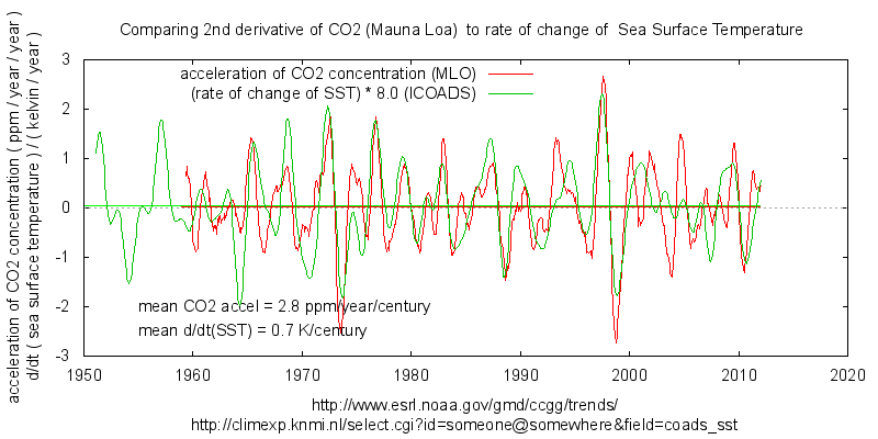
https://climategrog.wordpress.com/d2dt2_co2_ddt_sst-2/
The T vs dCO2 ratio is different at different times scales: less for longer time-scales. This is also expected in the presence of a relaxation to a new equilibrium change.
Inter-decadal ratio is about twice the inter-annual ratio.
Is this the first time this has been presented? If so, this is quite significant. And I do understand the limitations of short term correlations. It is still compelling.
Anyone, what is the time offset between the temp and delta CO2?
dCO2 vs T shows no lag. It is in phase. See my previous graph. The short term scales at 8 ppmv/y/K
The short term variability is largely ( though not enitrely ) explained as T driving rate of change in CO2. That relationship has been known for a long time. Though some of the erroneous claims I’ve pointed out above may be “new”.
To match the inter-decadal variabililty it needs scaling as ppmv/y/K
https://climategrog.wordpress.com/ddt_co2_sst/
That does not “prove” anything , it is just arbitrarily scaled for exploratory purposes.
Here’s the graph:
Greg, these upcoming years could very well prove something… If we see anticpated cooling (knock on wood) and the carbon growth rate falls with temperature, then that would do it. On the other hand if temps and growth rate part ways, that will tell us something, too. i hope something happens, because the suspense is killing all the climate change junkies here at wuwt. (as evidenced by all the above comments!)…
So much chatter about CO2, yet we see a blip in the Lapse rate from…. Ozone. doh!
In regards to Figure 2, whenever one plots CO2 and temperature on the same graph, the scaling of the axes gives you an implied climate sensitivity, i.e., you can ask: What sort of sensitivity would be necessary to have the CO2 and temperature graphs align? The answer for this graph is that it would require a temperature increase of 17 C per CO2 doubling.
Since we are talking about a temperature rise that has not yet equilibrated, this number is most properly compared to the TCR (transient climate response). The average TCR for the models in IPCC AR5 looks to be about 1.8 C per CO2 doubling. [See Figure 9.42(b) in the Working Group 1 report.] Hence, the scaling on the graph is such that alignment would occur if the TCR in the real climate system were an order of magnitude larger than the models predict.
So, what we learn from the graph is that the TCR is nowhere near 10 times what it is expected to be. We also learn once again how easy it is to confuse people with poorly designed graphics (whether done for the purposes of intentional deception or out of ignorance).
“The answer for this graph is that it would require a temperature increase of 17 C per CO2 doubling.”
Que?!
“Since we are talking about a temperature rise that has not yet equilibrated”
Sure. Not yet “equilbriated”? For a hamburger today, I will gladly repay you two on Tuesday!
Bartleby:
You can get the implied climate sensitivity of the graph by noting, for example, that a temperature rise from 0 to 5 degrees on the left scale is equated to a CO2 rise from 345 ppm to 420 ppm on the right scale. The formula to get the sensitivity for doubling the concentration is then given by [5 degrees/ln(420/345)]*ln(2). This gives you 17.6 C per doubling. As Phil. below notes, CO2 concentration should really be plotted on a log scale here…And because it isn’t, the result you get will depend slightly on the range you use. For example, if you note that 1 deg is equated to a CO2 rise from 345 to 360 ppm, you get [1 degree/ln(360/345)]*ln(2) = 16.3 C per doubling. But, basically, the answer will be around 17 C per doubling, plus or minus about a degree or two.
Not really sure what your point about hamburgers is.
Joel writes: “You can get the implied climate sensitivity of the graph by noting, for example, that a temperature rise from 0 to 5 degrees on the left scale is equated to a CO2 rise from 345 ppm to 420 ppm on the right scale.”
I suppose this is where I lost the thread of reasoning; I looked at the graph as a simple duel axis, not meant to imply a relation, rather to demonstrate the lack of one. I had no urge to imply a climate sensitivity by equating the axis. I don’t understand why the graph implies a climate sensitivity at all, or to what.
Joel –
After starring at the graph for awhile longer with the idea of “sensitivity” in mind I think I may have an idea of what you’re trying to say; the x-axis for CO2 is expanded in a way that leads to an incorrect assumption temperature isn’t sensitive to it. By using a large x-axis range the relation (if any) is hidden.
I assume you were using irony to point this out?
Bartleby – Yes, exactly. Like I said, that graph as been designed so that it illustrates the the climate sensitivity (transient climate response, TCR) is nowhere near 17 C per CO2 doubling. However, nobody was ever claiming that it was anywhere near it. If it were properly scaled so that the two curves aligned for a TCR of 1.8 C per doubling, then in fact I think that the temperature and CO2 curves would align much better (at least the trend part of the temperature…Of course there are large fluctuations in temperature due to other factors and, as someone has pointed out, these are especially pronounced when you look at lower tropospheric temperatures measured by satellites rather than global surface temperature).
Joel; sorry, I meant to write “the x-axis for temperature is expanded…” If the range of temperature on the left axis was -1 to 1 for example, the slope would change and the implication of decoherence would be reduced. That would most certainly effect the “implied sensitivity” you discuss.
I think you more or less put your finger on why I was having difficulties with that graph (assuming of course I actually discovered what you were trying to say). Thanks.
BTW, the “hamburger” comment was an obtuse (meant to be humorous) reference to the idea the effects of rising temperature and carbon where being observed in a system not “yet” in equilibrium. “For one hamburger today, I will gladly repay you two on Tuesday” is a forward looking description of a system not in equilibrium, as expressed by the great physicist Wimpy, of Popeye fame.
What we learn from Figure 2 is that the author doesn’t know what he’s talking about since the plot should be vs Log(CO2). If you applied your analysis to a correct graph Joel I expect that you would have a rather different answer.
Actually that’s somewhat of a red herring, Phil. The difference between a linear scale and a log scale when you have just plotted CO2 concentration over the range 330 to 420ppm is quite small. (If he had plotted it over a considerably broader range, then yes, that would be a problem.) My point still stands…and my quantitative estimate of the implied climate sensitivity is certainly good to within 10%.
This all does seem to confirm that temperature is a driver of CO2 but , as Duncan’s
December 16, 2016 at 6:23 pm graph shows , it is far from explain the increase in CO2 . In fact to really put things in proper perspective , where % increase in CO2 can related to % increase in temperature , temperature must be expressed in Kelvin . On such a % per % scale its clear that
dT/dCO2concentrationis so near 0. that on the same scale the change in temperature are virtually invisible as in this overview graph : http://cosy.com/Science/CO2vTkelvin.jpg .But my real objection is the statement of the IPCC paradigm :
In fact the radiative balance temperature of the lumped earth+atmosphere spectrum is about 23 degrees below the gray body ~ 278 in our orbit . And it is claimed that earth+atmosphere spectrum is significantly determined by the atmosphere . It would indeed seem odd that the surface alone would be so far from gray , far more absorptive=emissive in the IR than the surface to cause that 9% reduction from the gray body temperature ( 30% reduction in power ) , but I have never seen the two spectra factored .
In any case , the Divergence Theorem , and the symmetry electromagnetic interactions would seem to preclude spectral effects from explaining the 62% difference in energy density between that temperature and our estimated 288 surface temperature .
And I have never seen the differential which quantitatively explains that gap . The only applicable differential I know of is the Schwarzschild absorption differential , and altho I have higher priorities than implementing and exploring its parameter space to be sure , I am highly dubious that it can explain the spectral “trapping” of energy . In any case , in the more than a decade that I have been diverted by this AlGore-JamesHansen Warming assertion , I have never seen either equation quantitatively expressing the asserted physics nor an experimental demonstration of the phenomenon .
It is a paradigm without a quantitative analytical foundation .
There is no way in the world that even if the correlation between the dCO2/dt and GTA was perfect that the measured values could be this good. Not much has been made of this
http://woodfortrees.org/graph/hadsst3nh/mean:12/from:1960/plot/hadsst3sh/mean:12/from:1960/plot/hadsst2nh/mean:12/from:1960/plot/hadsst2sh/mean:12/from:1960
I’m suspecting that NH SST were used in calculation of CO2 levels and that might have become more obvious if a mistake wasn’t made.
Robert B,
The near-perfect releationship of the variability in CO2 rate of change and the temperature variability is the result of the fast response of tropical vegetation to (ocean) surface temperatures and following rain patterns. That gives some +/-1.5 ppmv around the trend. That says next to nothing about the cause of the trend, which is not caused by vegetation, as that is a small but growing net sink for CO2 over periods longer than 3 years…
See Pieter Tans at the festivities of 50 years Mauna Loa observatory, from sheet 11 on:
https://esrl.noaa.gov/gmd/co2conference/pdfs/tans.pdf
That vegetation is dominant can be seen in the opposite CO2 and δ13C changes. If the oceans were dominant, CO2 and δ13C changes would parallel each other…
Even if it were true, could both CO2 levels and SST be measured so well to see a good correlation?
“The near-perfect releationship of the variability in CO2 rate of change and the temperature variability is the result of the fast response of tropical vegetation to (ocean) surface temperatures and following rain patterns.”
No, it is due to differential flux in the natural flows, modulated by temperatures. This accounts for both the variability and the trend.
“That vegetation is dominant can be seen in the opposite CO2 and δ13C changes. If the oceans were dominant, CO2 and δ13C changes would parallel each other…”
This is a very complicated diffusion process. We can make no conclusions about the source of the rise from the δ13C data. It is consistent with your narrative, but it is consistent with other scenarios as well.
Bartemis,
Here the graph of the opposite CO2 and δ13C over the 1991 Pinatubo and 1998 El NIño episodes:
http://www.ferdinand-engelbeen.be/klimaat/klim_img/temp_dco2_d13C_mlo.jpg
There are only two known huge sources of low-13C on earth: current organics and fossil organics. All inorganics (oceans, volcanic vents, carbonate rocks,…) are (much) higher in 13C/12C ratio. Thus any substantial release of CO2 from the ocean’s unbalance would increase the δ13C level of the atmosphere and the CO2 changes and δ13C changes would parallel each other. Any unbalance either way in the biosphere will give opposite changes of CO2 and δ13C, which is the case over the past decennia.
There is simply no alternative explanation, just like there is no alternative explanation for a lower pH if you add an acid to a solution…
Thus a temperature change gives a CO2 change in the same direction (with a small lag) and an opposite δ13C change in exact timing with the CO2 change.
That means that almost all of the variability in CO2 rate of change is caused by the short term response of (tropical) vegetation to temperature changes.
As the biosphere as a whole is a net sink for CO2 over periods longer than 1-3 years, based on the oxygen balance, that is not the cause of the trend. Slope and variability in CO2 rate of change are from different, independent processes and the “common” factor is just coincidence (and not even that good…).
Even so, the slope still may have been caused by the temperature increase, but that T slope and variabilty can be matched with CO2 slope and variability is only a valid argument for the variability, not for the slope…
To establish causality is often impossible. To establish control is sometimes possible.
“Thus any substantial release of CO2 from the ocean’s unbalance would increase the δ13C level of the atmosphere and the CO2 changes and δ13C changes would parallel each other.”
Again, this is only narrative. You have no actual proof. You are making an argument on what you find intuitively plausible. But, time and again, science has shown that intuition is not generally a strong guide to truth.
“There is simply no alternative explanation…”
Famous last words in science, just before a paradigm is upended…
Bart,
I know, any argument that doesn’t fit your theory must be wrong, insufficient, a narrative, not verified…
All what you have shown is that you have no idea what the opposite CO2 and δ13C means: that is solid proof that vegetation is the main reactant to the temperature variability, far more than the oceans.
As solid as looking at a pH and conclude that an acid was added to a solution if the pH gets lower…
That is a huge problem for your theory, as that proves that variability and slope are not caused by the same processes and that your one-factor-fits-all is pure coincidence…
These things are important, Ferdinand. This is the scientific method. You do not make conclusions based on evidence which cannot be verified, or which is merely consistent with your hypothesis, but not uniquely so. This is faulty reasoning, and has led to repeated failures of science in the past.
Science is hard. We are not more scientific than our predecessors because we have more technological gadgets. We are more scientific because we have evolved a system of rigorous logic embodied in the scientific method that prevents (or, at least steers us away from) commiting the errors of the past. When you engage in slipshod rationalization like this, you are no better than the witch doctors who pronounced the gods angry because the crops failed, or the volcano rumbled.
Bartemis:
These things are important, Ferdinand. This is the scientific method. You do not make conclusions based on evidence which cannot be verified, or which is merely consistent with your hypothesis, but not uniquely so.
Well Bart, I have been about half my working life a (chemical) process engineer, upgrading new products from laboratory scale to 17 tons batches. Of course such an upgrade has its problems and that was my job to find out what the causes of the problems were, indeed by using the scientific method: looking at the possible causes of the problems, or better and much faster: eliminating the impossible causes.
All what you have is match between two variables, of which one part – the variability – is real, the other part – the match of the slopes – is largely bogus.
The evidence is that the variability in rate of change of CO2 after the variability of a temperature rate of change is mainly caused by the reaction of tropical vegetation on changed temperature and rain patterns.
The evidence is that the slope in rate of change of CO2 is not caused by the influence of the temperature increase on vegetation, as the biosphere as a whole is a small, but growing, sink for CO2.
Thus variability and slope are caused by different processes.
Still, the increase in sea surface temperature may have triggered more CO2 releases from the oceans.
Further we have human emissions which are average twice the observed increase in the atmosphere.
That means that the slope in the CO2 rate of change is not uniquely attributable to the temperature increase and that we have to look for more observations to decide which one is dominant.
Your theory completely is “inconsistent” with all known observations, while my theory is “consistent” with every single observation.
Using the scientific method, your theory is completely refuted…
If you can show me where my reasoning is wrong or why the sea surface temperature is the unique driver without violating any observation, I am all ear…
“All what you have is match between two variables, of which one part – the variability – is real, the other part – the match of the slopes – is largely bogus.”
You haven’t a smidgeon of evidence to make that claim. It is a near perfect fit. That is not happenstance. It is the same process. The phase match is coherent all the way down to the lowest observable frequencies. It violates no observation, only your interpretation of the given observation.
Oh…and for those wondering if the relationship between temperature and rate of change of CO2 in the modern record, as shown in Figure 1, is a new discovery, the answer is that it is not. It was first pointed out 25 years ago in this paper: J. B. Marston, M. Oppenheimer, R. M. Fujita, and S. R. Gaffin,”CO2 and Temperature,” Nature 349, 573 — 574 (1991). I couldn’t find a version of the paper that is not behind a paywall, but here is a NY Times article from the time discussing it: http://www.brown.edu/Research/bradmarston/Professor_Marston/Publications_files/carbon_cycle.jpg
The “theory” that is referenced by the NY Times article is nothing more than a conjecture. As this conjecture is not falsifiable there is not a way in which it can be elevated to the level of a “theory.”