October to December 2011 NODC Ocean Heat Content Anomalies (0-700Meters) Update and Comments

Guest post by Bob Tisdale

SAME INTRODUCTION AS ALWAYS

The National Oceanographic Data Center’s (NODC) Ocean Heat Content (OHC) anomaly data for the depths of 0-700 meters are available through the KNMI Climate Explorer Monthly observations webpage. The NODC OHC dataset is based on the Levitus et al (2009) paper “Global ocean heat content (1955-2008) in light of recent instrumentation problems”. Refer to Manuscript. It was revised in 2010 as noted in the October 18, 2010 post Update And Changes To NODC Ocean Heat Content Data. As described in the NODC’s explanation of ocean heat content (OHC) data changes, the changes result from “data additions and data quality control,” from a switch in base climatology, and from revised Expendable Bathythermograph (XBT) bias calculations.

The NODC provides its OHC anomaly data on a quarterly basis. At the NODC website it is available globally and for the ocean basins in terms of 10^22 Joules. The KNMI Climate Explorer presents the quarterly data on a monthly basis. That is, the value for a quarter is provided for each of the three months that make up the quarter, which is why the data in the following graphs appear to have quarterly steps. Furnishing the OHC data in a monthly format allows comparisons to monthly datasets. The data is also provided on a Gigajoules per square meter (GJ/m^2) basis through the KNMI Climate Explorer, which allows for direct comparisons of ocean basins, for example, without having to account for surface area.

This update includes the data through the quarter of October to December 2011.

Let’s start the post with a couple of looks at the ARGO-era OHC anomalies.

ARGO-ERA OCEAN HEAT CONTENT MODEL-DATA COMPARISON

I’ve started the post with a graph that gets people riled up for some reason.

Figure 1 compares the ARGO-era Ocean Heat Content observations to an extension of the linear trend of the climate models presented in Hansen et al (2005) for the period of 1993 to 2003. Over that period, the modeled OHC rose at 0.6 watt-years per year. I’ve converted the watt-years to Gigajoules using the conversion factor readily available through Google: 1 watt years = 31,556,926 joules. Even with the recent uptick in Global Ocean Heat Content anomalies, the trend of the GISS projection is still 3.5 times higher than the observed trend.
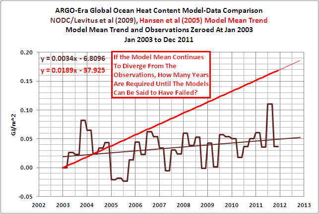
Figure 1

################################

STANDARD DISCUSSION ABOUT ARGO-ERA MODEL-DATA COMPARISON

Many of you will recall the discussions generated by the simple short-term comparison graph of the GISS climate model projection for global OHC versus the actual observations, which are comparatively flat. The graph is solely intended to show that since 2003 global ocean heat content (OHC) anomalies have not risen as fast as a GISS climate model projection. Tamino, after seeing the short-term model-data comparison graph in a few posts, wrote the unjustified Favorite Denier Tricks, or How to Hide the Incline. I responded with On Tamino’s Post “Favorite Denier Tricks Or How To Hide The Incline”. And Lucia Liljegren joined the discussion with her post Ocean Heat Content Kerfuffle. Much of Tamino’s post had to do with my zeroing the model-mean trend and OHC data in 2003.

While preparing the post GISS OHC Model Trends: One Question Answered, Another Uncovered, I reread the paper that presented the GISS Ocean Heat Content model: Hansen et al (2005), Earth’s energy imbalance: Confirmation and implications”.Hansen et al (2005) provided a model-data comparison graph to show how well the model matched the OHC data. Figure 2 in this post is Figure 2 from that paper. As shown, they limited the years to 1993 to 2003 even though the NODC OHC data starts in 1955. Hansen et al (2005) chose 1993 as the start year for three reasons. First, they didn’t want to show how poorly the models hindcasted the early version of the NODC OHC data in the 1970s and 1980s. The models could not recreate the hump that existed in the early version of the OHC data. Second, at that time, the OHC sampling was best over the period of 1993 to 2003. Third, there were no large volcanic eruptions to perturb the data. But what struck me was how Hansen et al (2005) presented the data in their time-series graph. They appear to have zeroed the model ensemble mean and the observations at 1993.5. The very obvious reason they zeroed the data then was so to show how well OHC models matched the data from 1993 to 2003.

Figure 2

################################

The ARGO-era model-data comparison graph in this post, Figure 1, is also zeroed at a start year, 2003, but I’ve done that to show how poorly the models now match the data. I’m not sure why my zeroing the data in 2003 is so difficult for some people to accept. Hansen et al (2005) zeroed at 1993 to show how well the models recreated the rise in OHC from 1993 to 2003, but some bloggers attempt to criticize my graphs when I zero the data in 2003 to show how poorly the models match the data after that. The reality is, the flattening of the Global OHC anomaly data was not anticipated by those who created the models. This of course raises many questions, one of which is, if the models did not predict the flattening of the OHC data in recent years, much of which is based on the drop in North Atlantic OHC, did the models hindcast the rise properly from 1955 to 2003? Apparently not. This was discussed further in the post Why Are OHC Observations (0-700m) Diverging From GISS Projections?

HOW LONG UNTIL THE MODELS ARE SAID TO HAVE FAILED? (STANDARD DISCUSSION)

I asked the question in Figure 1, If The Observations Continue To Diverge From The Model Projection, How Many Years Are Required Until The Model Can Be Said To Have Failed? I raised a similar question in the post 2nd Quarter 2011 NODC Global OHC Anomalies, and in the WattsUpWithThat cross post Global Ocean Heat Content Is Still Flat, a blogger stated, in effect, that 8 ½ years was not long enough to reject the models.If we scroll up to Figure 2 [Figure 2 from Hansen et al (2005)], we can see that Hansen et al (2005) used only 11 years to confirm their Model E hindcast was a good match for the Global Ocean Heat Content anomaly observations. Can we then assume that the same length of time will be long enough to say the model has failed during the ARGO era?

And as noted in a number of recent OHC updates, it’s really a moot point. Hansen et al (2005) shows that the model mean has little-to-no basis in reality. They describe their Figure 3 (provided here as my Figure 3 in modified form) as:

“Figure 3 compares the latitude-depth profile of the observed ocean heat content change with the five climate model runs and the mean of the five runs. There is a large variability among the model runs, revealing the chaotic ‘ocean weather’ fluctuations that occur on such a time scale. This variability is even more apparent in maps of change in ocean heat content (fig. S2). Yet the model runs contain essential features of observations, with deep penetration of heat anomalies at middle to high latitudes and shallower anomalies in the tropics.”

I’ve deleted the illustrations of the individual model runs in my Figure 3 for an easier visual comparison of the graphics of the observations and the model mean. I see no similarities between the two. None.

Figure 3

BASIN TREND COMPARISONS

Figures 4 and 5 compare OHC anomaly trends for the ocean basins, with the Atlantic and Pacific Ocean also divided by hemisphere. Figure 4 shows the ARGO-era data, starting in 2003, and Figure 5 covers the full term of the dataset, 1955 to present. The basin with the greatest short-term ARGO-era trend is the Indian Ocean, but it has a long-term trend that isn’t exceptional. (The green Indian Ocean trend line is hidden by the dark blue Arctic Ocean trend line in Figure 5.)

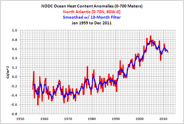
STANDARD NOTE ABOUT THE NORTH ATLANTIC: The basin with the greatest rise since 1955 is the North Atlantic, but it also has the largest drop during the ARGO-era. Much of the long-term rise and the short-term flattening in Global OHC are caused by the North Atlantic. If the additional long-term rise and the recent short-term decline in the North Atlantic OHC are functions of additional multidecadal variability similar to the Atlantic Multidecadal Oscillation, how long will the recent flattening of the Global OHC persist? A couple of decades?

Note also in the ARGO-era graph, Figure 4, that, in addition to the North Atlantic, there are three other ocean basins where Ocean Heat Content has dropped during the ARGO era: the North Pacific, South Pacific, and Arctic Oceans. We could assume the Arctic data is, in part, responding to the drop in the North Atlantic. But that still leaves the declines in the North and South Pacific unexplained.

Figure 4

################################

Figure 5

################################

Further discussions of the North Atlantic OHC anomaly data refer to North Atlantic Ocean Heat Content (0-700 Meters) Is Governed By Natural Variables. And if you’re investigating the impacts of natural variables on OHC anomalies, also consider North Pacific Ocean Heat Content Shift In The Late 1980s and ENSO Dominates NODC Ocean Heat Content (0-700 Meters) Data.

GLOBAL

The Global OHC data through December 2011 is shown in Figure 6. Even with the recent correction and uptick in the two quarters of this year, Global Ocean Heat Content continues to be remarkably flat since 2003, especially when one considers the magnitude of the rise that took place during the 1980s and 1990s.

Figure 6

################################

TROPICAL PACIFIC

Figure 7 illustrates the Tropical Pacific OHC anomalies (24S-24N, 120E-90W). The major variations in tropical Pacific OHC are related to the El Niño-Southern Oscillation (ENSO). Tropical Pacific OHC drops during El Niño events and rises during La Niña events. As discussed in the updates since late last year, the Tropical Pacific has not as of yet rebounded as one would have expected during the 2010/11 and 2011/12 La Niña events. In other words, the 2010/11 and 2011/12 La Niña events have done little to recharge the heat discharged during the 2009/10 El Nino.

Figure 7

################################

For more information on the effects of ENSO on global Ocean Heat Content, refer to ENSO Dominates NODC Ocean Heat Content (0-700 Meters) Data and to the animations in ARGO-Era NODC Ocean Heat Content Data (0-700 Meters) Through December 2010.

THE HEMISPHERES AND THE OCEAN BASINS

The following graphs illustrate the long-term NODC OHC anomalies for the Northern and Southern Hemispheres and for the individual ocean basins.

(8) Northern Hemisphere

#################################

(9) Southern Hemisphere

#################################

(10) North Atlantic (0 to 70N, 80W to 0)

#################################

(11) South Atlantic (0 to 60S, 70W to 20E)

#################################

(12) North Pacific (0 to 65N, 100 to 270E, where 270E=90W)

#################################

(13) South Pacific (0 to 60S, 120E to 290E, where 290E=70W)

#################################

(14) Indian (60S-30N, 20E-120E)

#################################

(15) Arctic Ocean (65 to 90N)

#################################

(16) Southern Ocean (60 to 90S)

HHHHHHHHHHHHHHHHHHHHHHHHHHHHHH

ABOUT: Bob Tisdale – Climate Observations

SOURCE

All data used in this post is available through the KNMI Climate Explorer:

http://climexp.knmi.nl/selectfield_obs.cgi?someone@somewhere

0 0 votes
Article Rating
86 Comments
Oldest
Newest Most Voted
Inline Feedbacks
View all comments
diogenes
January 26, 2012 4:17 pm

nice graph, Bob

markus
January 26, 2012 5:22 pm

No doubt about it Bob, the oceans are one of the most beautiful things in our ecological sphere.
We really should be caring for them, ultimately, without them, we wouldn’t have an atmosphere.
Markus Fitzhenry.

James Crawford
January 26, 2012 5:25 pm

Think about the magnitude of the heat increase, about Six Watt-Years per square meter over one decade.
This is only .6 W-yr/yr
Average insolation is about 350 Watt-Years per Year.
In other words, the net increase of heat influx to the oceans was about one tenth of one percent. This is trivial.

January 26, 2012 5:25 pm

You all know me by now…a bit slow on the uptake…so please explain to me very gently how all the alleged melt water from the melting ice pack and ice sheets is gently warming up the oceans?

Lew Skannen
January 26, 2012 5:28 pm

“HOW LONG UNTIL THE MODELS ARE SAID TO HAVE FAILED?”
I was always under the impression that if the observations strayed outside the error bars of the model then the model had failed.
I notice, however, that very few CAGW predictions come with error bars…

John F. Hultquist
January 26, 2012 5:30 pm

Bob asks:
If The Observations Continue To Diverge From The Model Projection, How Many Years Are Required Until The Model Can Be Said To Have Failed?
“There you go again.” (R.R., 1980)
Expecting “the team” to capitulate will likely mean a long wait. Many scientific debates do not end until the elderly, with much invested, have left the scene.

January 26, 2012 5:45 pm

Lew Skannen says:
“I notice, however, that very few CAGW predictions come with error bars…”
And I notice that no CAGW predictions come true. Ever.

John F. Hultquist
January 26, 2012 5:49 pm

Charles Gerard Nelson says: @5:25.
You are supposed to use ‘sarc’ on things like that.
Nevertheless, I will still suggest a two-part exercise. Find a globe. Put your cusped hand over the Arctic and then do the same for Antarctica. Now put the heal of your palm on the globe near Peru and step by step move it until you have covered the ocean to the east coast of Africa. Part 2: Find a true color photo of the ocean from space with the sun directly above the camera’s viewpoint. What color does the ocean appear? With respect to solar energy, what does that “color” imply?

Steptoe Fan
January 26, 2012 5:55 pm

with limited memory ( before ) in my laptop, the Argo tools and data set produced graphs that convinced me of the fact that the Pacific ocean was really holding trivial, if any, heat.
now, that I have a full 2 GB, will have to re explore with the tools. with Argo, more memory is better ( much more ).
thanks for your post.

Alan Statham
January 26, 2012 6:10 pm

Without uncertainty estimates on both the models and the observations, you cannot meaningfully compare the two. You show no uncertainty estimates at all in this post. You don’t even use the word “uncertainty”. Ergo, nothing meaningful here.

John F. Hultquist
January 26, 2012 6:14 pm

Steptoe Fan says:
January 26, 2012 at 5:55 pm
“ . . . holding . . . heat.

Put some of that 2 GB to good use and store the meanings of heat and enthalpy.

Braddles
January 26, 2012 6:17 pm

Seriously Bob, you need some advice on how to present information with impact.Those first two paragraphs are turgid waffle of virtually no interest to most readers, followed by a long data dump. Most of it reads like an appendix to some report. This isn’t some hidebound old scientific journal where you are trying to impress a handful of readers with your erudition.
Come up with two or three succinct talking points, supported by one or two critical graphs or summary tables. For those who want to study the detail, append it after you state your findings, or better still link to it somewhere else.

Brian H
January 26, 2012 6:22 pm

Actually, you just need to keep expanding the error bars around the estimates to accommodate the latest reading. That way, the models are always right, just more and more dubiously! Simples.

David A. Evans
January 26, 2012 6:24 pm

1st let me protest the use of heat content. It’s energy content in Joules.
Correct me if I’m wrong. For whatever reason, the energy content of the Equatorial Pacific is not recharging as it should during this La Niña. What does this mean for the energy content after the next El Niño?
Surely a further reduction in overall Ocean energy content.
As most of the retained energy in the system is in the oceans, this must imply cooling!
DaveE.

Mooloo
January 26, 2012 6:37 pm

Alan Statham says:
Without uncertainty estimates on both the models and the observations, you cannot meaningfully compare the two.

So you will believe Bob if he puts uncertainty bars on?
Or are you just looking for any excuse to fail to see the obvious divergence of model and reality?

DRE
January 26, 2012 6:46 pm

What is eleventy billion standard deviations Alex?

JJ
January 26, 2012 6:58 pm

Lew Skannen says:
I notice, however, that very few CAGW predictions come with error bars…

Not true, Lew. All CAGW predictions come with error bars. They just dont let people see them, until the discrepancy between their scare mongering and the unfudgable observations becomes so large as to be laughable. THEN they start talking about error bars, and using the term “consistent with” as if it means “proof”. This guy is halfway there already:
Alan Statham says:
Without uncertainty estimates on both the models and the observations, you cannot meaningfully compare the two.

Yes, Alan, you can. And you can also point at them and laugh.
Those scaremongering model predictions do not come anywhere close to the observations. And those observations are known to be far more accurate than the data that the scaremongering model predictions are based on. If the $#!^^y model based on the $#!^^y data is a factor of 3.5 off the better data, then we have no reason whatsoever to place any weight on those $#!^^y model predictions. If they are correct it will be by dumb luck, not knowledge and reason. And that is a very meaningful comparison.
You show no uncertainty estimates at all in this post. You don’t even use the word “uncertainty”. Ergo, nothing meaningful here.
LOL. NOW you guys have discovered the concept of “uncertainty”.
Now, follow the talking points and claim “consistent with”. C’mon. We know you want to.

Joachim Seifert
January 26, 2012 7:21 pm

Bob, since Hansen said the missing heat which is stuck in the pipeline since the OHC graph
turned flat in 2000 is not really stuck but hiding……
below your 700 m ocean depth ….. too bad……my question would be in which of the oceans
(and your graphs) would the hiding place of the heat be located…. since your graphs
stay flat…..? I always thought warm water comes up to the surface but now it goes down……

January 26, 2012 7:26 pm

I never see this point discussed, but it does relate to ocean heat content, so please bear with me in what will need a long explanation.
Suppose, for example, that the surface and oceans were to rise to some “equilibrium” of, say, 5 degrees warmer in say 200 years. You simply could not have a situation whereby temperatures, say, 100 metres underground (and under the floor of the oceans) remained at current levels. Unless those temperatures also rose by about 5 degrees you have no long term equilibrium.
Over the course of the life of the Earth its surface has reached its current temperatures at various points on the globe. Underground, coming from the core (about 5,700 deg.C) down to the surface we have a fairly linear temperature plot. At least we know from measurements what happens in the last few kilometres anyway, the deepest borehole being about 9Km. The lapse rate underground is about 30 deg.C per Km but my point is that the plots in numerous boreholes that I have analysed all extrapolate approximately to a “base” temperature which we would expect on a calm winter night at that point on the surface.
So we have a continuous temperature plot from the core to TOA with a kink in the gradient at the surface. But it’s only a kink in the gradient – not a 5 degree step, and never could be. (Of course there are daily variations as thermal energy on a sunny morning flows into the surface – and then back out again at night, and some hangs around from summer to winter. But there is a tendency to come back to the base at any particular location on calm winter nights. Think of the base as a sloping rock platform onto which we pour a bit of sand in the day which slides off in the night.)
Thermodynamics tells us that the underground plot would have to rise by 5 degrees at the surface end, assuming the core temperature stayed constant. This may seem strange to some, because it seems to imply that we need to send thermal energy uphill so to speak. But in fact it takes time – a long time – and the gap under the (new) line would be filled in by thermal energy coming from the core. This is a slow process. It may take thousands, or perhaps millions of years, I don’t know, but it would not happen in 200 years, that’s for sure.
Hence there would be a propensity for thermal energy from that wrongly named “ocean heat content” to flow under the floor of the ocean in an “effort” to equalise the temperatures. And that would lead to cooling of the oceans – a natural stabilising effect due in essence to the far greater thermal energy under the surface than anywhere in the oceans or land surfaces.
There is more detail on this stabilising “support mechanism” on this page of my site http://climate-change-theory.com/explanation.html
What do others think?

January 26, 2012 7:29 pm

Models should come in boxes or wear skimpy dresses – other than that, reality is destroying them every day.
Hey, Anthony – you have an Ozero campaign ad on this site? WUWT? You have officially ‘arrived’ – the Bamster’s campaign has figured out that this site has more traffic than UnRealclimate! 🙂

January 26, 2012 7:39 pm

What Bob has clearly show is these very expensive models are not better then any other prediction methodology based on inductive reasoning. Inductive logic is the hallmark of a priori reasoning not of the deductive logic of reasoned science. To those suffering from a massive attack of Cognitive Dissonance they will hold to their mythology for a very long and painful time.

Camburn
January 26, 2012 7:44 pm

Thank you Mr. Tisdale. And excellent update as always.

AJB
January 26, 2012 7:53 pm

Where in heck did “watt-years” come from? SI units like kWh and GWh I understand, is this some new fudge-factorable Hansenian unit?
No wonder that graph gets people riled up. How many seconds are there in a year?
January 2nd, February 2nd, March 2nd… so 1 watt-year = 12 joules, right?
Oh! wait … I get it now. A watt-year is the amount of energy Anthony and gang expend running this blog for a year. Well, that’s way more than 31,556,926 joules, Bob. Better fix that graph, I think you’ve just found Trenberth’s missing heat and it’s worse than we thought! 🙂

January 26, 2012 7:57 pm

The poles are still frozen. From the above synopsis, the oceans are not even 1 C warmer in the time frame given. So, it the Arctic average temperature goes up by such, what effect is it going to have??? Just move the Arctic temperature graphs up one degree ( http://ocean.dmi.dk/arctic/meant80n.uk.php ). The change is insignificant. The poles are still frozen.

Chad Jessup
January 26, 2012 8:43 pm

Bob, forget about what Alan says and keep posting those charts, as they help to visually understand your stated points.

Cecil Coupe
January 26, 2012 8:44 pm

I think the uncertainty bands are shown in the color white. Some would say that’s the background color but I think it’s are the error range.

January 26, 2012 9:17 pm

highflight56433 says:
“The poles are still frozen.”
The melting of ice in the Arctic is more likely to be affected by the temperatures of the Arctic Ocean and the North Atlantic Ocean which feeds it. This is because more floating ice melts from the underneath side and the rate of melting depends on the temperature of the water and also the rate of flow. Both follow natural cycles like ENSO.
Melting by the Sun obviously only happens in summer, but much of its radiation is reflected away. And as for any backradiation – well we’ve seen that it can’t even melt a bit of frost. http://climaterealists.com/index.php?id=9004
The above plots for these oceans appear to have passed maxima in 2004 and are now declining,

u.k.(us)
January 26, 2012 9:31 pm

Braddles says:
January 26, 2012 at 6:17 pm
Seriously Bob, you need some advice on how to present information with impact.Those first two paragraphs are turgid waffle of virtually no interest to most readers, followed by a long data dump. Most of it reads like an appendix to some report. This isn’t some hidebound old scientific journal where you are trying to impress a handful of readers with your erudition.
Come up with two or three succinct talking points, supported by one or two critical graphs or summary tables. For those who want to study the detail, append it after you state your findings, or better still link to it somewhere else.
=============
Umm,
Bob Tisdale produces graphs you would never see otherwise, links are provided.
If looking for a “finding”, you have the wrong man.
All you are going to get are the facts, by the truckload.

Steptoe Fan
January 26, 2012 9:39 pm

actually John F, I think I’ll go with David A and replace ‘heat’ with ‘energy’, and yes it is quite simplistic, my initial sentence. do you have it in your capacity to dole out forgiveness, as the climate gods are supposedly want to do ?

phlogiston
January 26, 2012 11:05 pm

As discussed in the updates since late last year, the Tropical Pacific has not as of yet rebounded as one would have expected during the 2010/11 and 2011/12 La Niña events. In other words, the 2010/11 and 2011/12 La Niña events have done little to recharge the heat discharged during the 2009/10 El Nino.
Are we talking about “La Nina Modoki”?
Thanks for the update Bob, please keep them coming, this is important stuff. As u.k.(us) says, you wont find this anywhere else (except hidden in technical web pages under a cloak of political invisibility).

Stephen Wilde
January 26, 2012 11:18 pm

Bob,
Could you summarise what you see as the implications of the data that you have presented ?
I am particularly interested in whether you think the ocean energy content has recharged as much as you think it ‘should’ have done during the recent La Nina.
If not, then the choice is between the Svensmark idea of more cosmic rays seeding more clouds and my idea of a less active sun pushing the jetstreams equatorward and/or making them track more meridionally to create more clouds.

January 27, 2012 12:17 am

I do not believe Argo, or its data processing. Every update made from post-2003 decline has created and increase from original decrease.
http://earthobservatory.nasa.gov/Features/OceanCooling/
Belief of Argo authors is stronger than reality.

Editor
January 27, 2012 1:37 am

Stephen Wilde says: “Could you summarise what you see as the implications of the data that you have presented ?” And you clarified, “I am particularly interested in whether you think the ocean energy content has recharged as much as you think it ‘should’ have done during the recent La Nina.”
Stephen, to discuss those matters, I would need updated cloud amount data (ISCCP) and downward shortwave radiation data at the surface. Presently they are not available (in an easy-to-use format). And a clarification: It’s not that the tropical Pacific OHC did not recharge as I think it should have during the 2010/11 La Nina. It did not recharge at all. Based on past performance, tropical Pacific OHC should have risen in response to 2010/11 La Nina, but it did not; it continued to drop as though the El Nino continued into the 2010/11 ENSO season.

Stephen Wilde
January 27, 2012 2:05 am

Thanks Bob,
That reply gives me enough to go on because you confirm the lack of recharge.
My opinion (not yet proved by good enough data) is that the more meridional/equatorward jets and climate zones have led to more cloudiness with a reduction of solar energy into the oceans.
The Earthshine data does suggest increasing global cloudiness since around 2000 which was about when I first noticed that the jets had stopped moving poleward.
During the late 20th century we had a decrease in cloudiness, more poleward jets and rising ocean energy content.
So, as things are at present, there is real world support for my suppositions/speculations.

Stephen Wilde
January 27, 2012 2:08 am

And if reduced solar input to the oceans is the culprit then most likely that is also responsible for skewing ENSO in favour of La Nina.

Editor
January 27, 2012 2:17 am

Braddles: This post is a data update. The NODC provided data for the months of October to December 2011, so I presented it. I provide the same thing every quarter but rearrange the post. It’s not a post about specific findings. Those I handle differently.
For example: the difference between Northern and Southern Hemisphere OHC (Northern Hemisphere OHC minus Southern Hemisphere OHC) appears to be influenced by ENSO.
http://i42.tinypic.com/dfy8ic.jpg
To me that’s newsworthy, since I’ve never seen it discussed in a paper or at a blog. That finding would be presented in a separate post with the data broken down into ocean basins, the tropics, etc., but I might mention the overall finding in an update as an intro to that separate post.

Robert of Ottawa
January 27, 2012 3:53 am

Can someone remind me of the story of the adjustment of the Argo data, I forget the details

Robert of Ottawa
January 27, 2012 3:55 am

Ah, read and ye shall find … thanks Juraj!
http://earthobservatory.nasa.gov/Features/OceanCooling/

Alan Statham
January 27, 2012 4:19 am

Mooloo: “…Or are you just looking for any excuse to fail to see the obvious divergence of model and reality?” – you miss the point by a huge margin. Without uncertainties, you can’t tell if there is an “obvious divergence”. You are just seeing what you want to see. In the real world, sensible people use appropriate tools to find out what the numbers are telling them, rather than simply slapping their own interpretation onto a partial data set.

Pamela Gray
January 27, 2012 6:40 am

But, Steven, as yet no mechanism with the math to back it up from you for your suppositions and speculations regarding some component of solar mechanics having to do with the shifting jets.

Grant
January 27, 2012 6:43 am

Braddles says:
January 26, 2012 at 6:17 pm
“Seriously Bob, you need some advice on how to present information with impact.Those first two paragraphs are turgid waffle of virtually no interest to most readers, followed by a long data dump. Most of it reads like an appendix to some report. This isn’t some hidebound old scientific journal where you are trying to impress a handful of readers with your erudition.”
Maybe Braddles should be reading USA Today? How bout a chimp in a checkered sports coat pointing to salient spots on the graphs?

Stephen Wilde
January 27, 2012 7:10 am

Pamela Gray,
Lots of circumstantial evidence with an outcome as I anticipated.
The mechanism has been described in detail elsewhere and simply relies on basic physical principles and fluid dynamics combined with empirical observations.

barry
January 27, 2012 7:19 am

I’m not sure why my zeroing the data in 2003 is so difficult for some people to accept.

If you’re talking about changing the baseline, then that’s no problem. But you’ve started the trend at a high point in the anomaly data instead of just continuing the trend from 1993, which would be a much better way to see if the prediction held up.
Here’s a trend line for UAH temp data from 1990. It’s an actual trend, but let’s call it a prediction.
http://www.woodfortrees.org/plot/uah/from:1990/mean:12/plot/uah/from:1990/trend
Now I’ll just ‘zero the data’ in 1998 and see what happens.
http://www.woodfortrees.org/plot/uah/from:1990/mean:12/plot/uah/from:1990/trend/offset:0.25
You reckon that’s kosher?
You can do the same trick to make it look as if the trend underestimates the observation.
http://www.woodfortrees.org/plot/uah/from:1990/mean:12/plot/uah/from:1990/trend/offset:-0.2
‘Zeroing’ the start of the trend (not ‘data’) from a high or low anomaly will skew the results, as you’ve done.

Jeff Alberts
January 27, 2012 7:47 am

Grant says:
January 27, 2012 at 6:43 am
Maybe Braddles should be reading USA Today? How bout a chimp in a checkered sports coat pointing to salient spots on the graphs?

ROTFL. Zing!

Septic Matthew
January 27, 2012 7:51 am

Braddles: Seriously Bob, you need some advice on how to present information with impact.
FWIW, I liked the presentation as is. Probably we all have our favorite formats, but I see no reason for Bob Tisdale to change his style.

Septic Matthew
January 27, 2012 8:07 am

barry: ‘Zeroing’ the start of the trend (not ‘data’) from a high or low anomaly will skew the results, as you’ve done.
If a report displays a model result based on data from year X0 to year X1, the obvious place for “zeroing” a display that is meant to test the model based on data after year X1, is year X1 — exactly as Bob Tisdale did. In this case, X0 is 1993, X1 is 2003, so 2003 is the ideal year for “zeroing” the graph (and all subsequent statistical analyses), exactly as Bob Tisdale did. It is a good practice to test a model based on data collected subsequent to the development of the model, exactly as Bob Tisdale did.
The fact is that the model that fit the 1993 – 2003 data has been a poor predictor of the years since then, exactly as Bob Tisdale showed. How long this divergence has to persist before the data substantiate rejection of the model at one of the conventional levels of statistical significance can be computed — assuming that the divergence actually persists, but we won’t know until after we have observed the next 2 decades’ worth of data, pretty much as Bob Tisdale wrote.
This is obviously not the last word, but it is the latest of many demonstrations that the models have no demonstrated predictive power. Enough of these, and almost everyone will come to realize and understand that the models have no predictive power.

J Bowers
January 27, 2012 8:44 am

“I’m not sure why my zeroing the data in 2003 is so difficult for some people to accept.”
Your not being sure why may be indicative of your problem. Tamino has given it it to you once again, BTW.

Louise
January 27, 2012 8:55 am
Utahn
January 27, 2012 9:02 am

I agree with Tamino here as well.
Bob, what do you think about his post?
http://tamino.wordpress.com/2012/01/27/fake-predictions-for-fake-skeptics/#more-4671

Doug Proctor
January 27, 2012 9:19 am

Comment 1: Data since +/-Y2000 doesn’t show a rise in OHC or temps, but if you consider from about 1983 foreward, and give some variance of a multi-year ups-and-down level, you can easily say that after the ’98 Pinatubo event there was a sudden heating event that took a few years to cool back to “normal”. Now is the time for the CAGW to show up again, but the last decade doesn’t mean that the warmists must ackowledge failure, in my view.
Comment 2: When will failure be recognizable? In three years, by my estimate.
By 2015 I think we will be in a position to say the myth is busted. The OHC, global temperatures and sea-levels will have to rocket after that to meet the alarmist projections of 2050 and 2100 – and it is the alarmist levels, not moderate rives, that constitute both the hype and the “science” of global warming.
The Global Warming science is rooted in extreme reaction to CO2 (by water vapour feedback). Without the extreme reaction, standard skeptic scientific rules apply. Not only will the least plausible scenario be well matched by 2015 (Hansen’s “C”), which says that there is no evidence in the prior 37 years that their feedback was right, but that in order for chaos to reign by 2050/2100, a much more extreme reaction must occur in the next 35/85 years. Which none of their theories promote.
Comment 3: I would like to say that in three years CAGW will die a miserable, embarrassing death. But I don’t believe that it will. I expect that Chinese coal plants and their sulphur emissions will be blamed/thanked for continued life on the planet in 2016 The Hansen/Gore story will be that we have an unexpected reprieve – proving chaos theory can work for us as well as against us, by the way – in which to develop non-fossil fuel technology so that we don’t NEED the crazy Chinese power plants to save us from hell-on-Earth.
Even Harold Camping, with God on his side, couldn’t have it as good as Jimmy and Al do.

January 27, 2012 9:36 am

Bob:
On the first graph in the article. Could you run a Standard Deviation for that data for that time period. (I presume it is discreet, and you’ll be too!).
Then compare with that upward trend line (even the low sloped on, the real one compared to the “model prediction”..
Then us SLUGS who believe in data NOISE and “significance” can sort out if we are going to put any SIGNIFICANCE into the data.
ALSO could you review the nature of the BOGUS 1955 to ARGO buoy data? Frankly I think anything before the Argo buoys is a meaningless fantasy!

Editor
January 27, 2012 9:51 am

J Bowers says: “Your not being sure why may be indicative of your problem. Tamino has given it it to you once again, BTW.
Louise says: “Bob – any comment on http://tamino.wordpress.com/2012/01/27/fake-predictions-for-fake-skeptics/”
Utahn says: “I agree with Tamino here as well. Bob, what do you think about his post?”
J Bowers, Louise and Utahn: I explained why I presented the ARGO-era data with the data zeroed at 2003 in the post. Refer to the heading of STANDARD DISCUSSION ABOUT ARGO-ERA MODEL-DATA COMPARISON. Tamino did not refer to my post in his, but assuming his post is a response to mine, it appears that Tamino only looked at the graph and failed to read my post. He did not respond to my explanation, which included how Hansen et al (2005) presented their data. The name Hansen does not appear once in Tamino’s post. Hansen et al zeroed their data in 1993 to show how good their model mean matches the data between 1993 and 2003. And I zeroed the data in 2003 to show how it failed afterwards. Tamino simply presented data as he wished to present it. Did he use the model projection? I don’t believe he did. So his post has no bearing on my graph.
He presented the data as he wanted and I presented it the way I wanted. His choice; my choice. Nothing more, nothing less. I have no need to waste my time responding to his nonsense, but if you feel it’s necessary, I will be happy to write a rebuttal. And if Anthony Watts elects to cross post my rebuttal, I reach a larger audience than Tamino does. Would you like me to write the rebuttal post? Bloggers here love to see Tamino-related posts.
BTW, J Bowers, Tamino may try to give it to me, as you say, but he fails every time.
And here’s a difference between Tamino and me. When I make a mistake, I accept it and I acknowledge it in the post and in a follow-up post. When Tamino makes a mistake, he does not acknowledge it and leaves the post untouched. That way, Tamino looks infallible to YOU who find him credible. But the rest of us understand his failings.
Ciao

Editor
January 27, 2012 10:40 am

Max Hugoson says: “On the first graph in the article. Could you run a Standard Deviation for that data for that time period. (I presume it is discreet, and you’ll be too!).”
The Standard Deviation for the global OHC data in Figure 1 is 0.028 GJ/m^2.
With respect to your request about the OHC before the ARGO era, I don’t know that I’ve written a post solely about the differences in the XBT-based and the ARGO-based data. The NODC has been making corrections to both since I’ve been following their OHC data. The ARGO data has better coverage, especially south of 30S. There’s very little XBT-based data in the mid-to-high latitudes of the Southern Hemisphere oceans before those ARGO floats started bobbing around. And the global coverage of source data gets worse as the data goes back in time.
I wouldn’t try to use any OHC data to determine, for example, how much heat was released from the tropical Pacific during the 1982/83, 1997/98, or 2009/10 El Nino events. But I do use the data to show that there was a response from the tropical Pacific OHC data to those El Ninos as we would expect. In all three cases, tropical Pacific OHC dropped.

Utahn
January 27, 2012 11:02 am

A rebuttal? Yes, I would appreciate it. If Hansen et al picked an anomalous start date to make it look like the models were better than they were, that would be cherry-picking. But two wrongs wouldn’t make a right!

phlogiston
January 27, 2012 1:21 pm

An interesting statistical study would be to compare periods where OHC was rising and when – as now – it is falling: and to look at the blogosphere musings on the OHC and specifically count the number of mentions of the phrase “error bars”. FWIW my prediction would be that frequency of the mention of “error bars” is inversely proportional to the rate and sign of change gradient, i.e. less frequent with rising OHC, more frequent when it is falling.
Why is there so much AGW jowl-flapping at Bob Tisdale’s meticulously collated and presented oceanographic data? It is not Bob Tisdale’s data, it comes from sources such as NODC and NOAA. Why shoot the messenger just because you dont like the message? Clearly the real world is a cold wind to the AGW theory compared to the warm sofa of climate modelling or simulation. As for Tamino, the only person he is “giving it to” is himself. “Giving it” is also something that can be modelled or simulated – and the AGW crowd are no doubt as energetic in simulating this as they are at simulating the climate.

barry
January 27, 2012 2:10 pm

If a report displays a model result based on data from year X0 to year X1, the obvious place for “zeroing” a display that is meant to test the model based on data after year X1, is year X1

Wrong! The obvious place to zero the beginning of the trend line from year X1 is where the previous one ended in year X1, not from a higher (or lower) point.

The fact is that the model that fit the 1993 – 2003 data has been a poor predictor of the years since then, exactly as Bob Tisdale showed

The correct thing to do would have been to continue the trend line from the original.. Tisdale’s response that he is ‘doing what Hansen did’ is strange. If he did what Hansen did, that trend line would be continued instead of taking a jump up the Y-axis.
The point is that the new trend line begins at a high anomaly point in the data, rather than at a ‘normal’, or average point. Of course the trend line is higher than obs!

barry
January 27, 2012 2:38 pm

And look at the model runs from the original – each run is centred on 1993 as well as the mean. The models were designed to run from 1993. If you want to test the predictive capability of the models, you have to start the trend line in 1993 – or if you want to do a ‘display’ of that trend prediction since 2003, the beginning still has to lie on the original. There is no particular reason to start a new trend line in 2003 you could start one in 2001, 2004 or 1997 etc), but they all have to be an extension of the original, or you are comparing different models.
In fact, there’s a very good reason to start the trend in 1993 and extend it further, rather than starting a new one at 2003 – we have more data, and the results will be less susceptible to interannual variability.
Tisdale’s rationale for doing what he did is weak. I would like to know why he didn’t simply extend the trend estimate and incorporate all the data since 1993. Generally speaking, more data is better.

Berényi Péter
January 27, 2012 4:12 pm

That’s what we are talking about. Average temperature of the upper 700 m of oceans has increased by hardly more than 0.1°C in 57 years.
Pretty easy to calculate. Mass of this layer is known, specific heat of water is given, therefore heat content anomaly can readily be converted to temperature anomaly.

jasonpettitt
January 27, 2012 4:47 pm

“He presented the data as he wanted and I presented it the way I wanted. His choice; my choice. Nothing more, nothing less. I have no need to waste my time responding to his nonsense”
~Bob Tisdale
Oh, so that’s how science works. I always wondered.
I thought maybe it might be because 1993 represents the very beginning of the satellite altimetre record (http://sealevel.colorado.edu/). I didn’t realise Hansen was “cherry picking” the entire data set just because that made the wiggly lines look more better.
Seriously guys, this stuff is just poor.

jasonpettitt
January 27, 2012 5:22 pm

Oh, and just in case anyone wonders why the satellite altimeter record (which starts in 1993) pertains to ocean heat content -> http://www.agu.org/pubs/crossref/2003/2002JC001619.shtml

January 27, 2012 5:31 pm

Bob:
Thanks for 0.028 !!! Makes my day. Tells me that with the exception of the end of 2011 blip, the other variations are meaningless.
AND, unless I am forgetting all my basic statistics, just because …let’s say the “probability” of the 2011 blip is 10% of all the distributed values, DOES NOT MEAN IT WON’T HAPPEN!
I’d put like 3SD’s (so +/- almost 0.1) on the whole graph to say….do we have any real “beyond the true distribution” values… Since the mean seems to be about 0.04, that means 0.14 to -0.06, on that basis the significance of these variations becomes ZERO!

Editor
January 27, 2012 6:27 pm

jasonpettitt says: “I thought maybe it might be because 1993 represents the very beginning of the satellite altimetre record (http://sealevel.colorado.edu/).”
Nope. Ocean Heat Content is a different dataset.

Septic Matthew
January 27, 2012 6:30 pm

barry: In fact, there’s a very good reason to start the trend in 1993 and extend it further, rather than starting a new one at 2003
That would make more sense to me if Bob Tisdale had the code that was used to generate the runs to 2003. But he didn’t, so projecting their trend beyond 2003 and comparing them to post-2003 data is sensible.
FWIW, Hansen’s projections in 1988 were based on an arbitrarily selected start point, the end of the post WWII downturn, and no one in the AGW community has ever complained about that. We now have more years of non-warming than we had of warming when the whole catastrophic warming campaign began. I am impatiently waiting for 2030 when we have decades of data to compare to the predictions made in 1988 – 2003. Bob Tisdale has merely presented the latest example of a model that overpredicted the subsequent trend of a duration approximately equal in length to the data that were used to support its initial publication. If the trend of consistently inaccurate predictions continues long enough, we shall have to conclude that we know the models are unreliable for policy use.

Editor
January 27, 2012 6:49 pm

barry says: The point is that the new trend line begins at a high anomaly point in the data, rather than at a ‘normal’, or average point. Of course the trend line is higher than obs!
When I first started plotting the comparison a couple of years ago, 2004 was the high anomaly point. That’s discussed in my first rebuttal to Tamino that’s linked in the post. Since I started presenting the short-term ARGO-era graph, the NODC has updated the dataset twice, causing 2003 to be the “high anomaly point”.
You wrote, “Tisdale’s response that he is ‘doing what Hansen did’ is strange. If he did what Hansen did, that trend line would be continued instead of taking a jump up the Y-axis.”
This is so simple that I can’t fathom why this is being discussed. Hansen et at zeroed their data at 1993 to show how their model projection aligned with the data for the period of 1993 to 2003. I chose to zero the data in 2003, the end year of the Hansen comparison, to show that the model projection now diverges from the data. And there’s no better way to show that divergence than to align the two datasets at the beginning of the period. That “v” laying on its side is precisely the image I was looking for. Hansen et al presented the data as they wanted, and I’ve presented as I wanted. You may not like the appearance of what I’ve done, but it is exactly the image I wanted to show.

jasonpettitt
January 27, 2012 7:18 pm

“Nope. Ocean Heat Content is a different dataset.”
~Bob Tisdale.
No it’s not. -> http://www.agu.org/pubs/crossref/2003/2002JC001619.shtml
Hansen used 1993 as a start point because that’s the very beginning of the data-set.
Hansen is right. Tamino is right. You’re wrong.
You’ve not justified “moving” Hansen’s projection. You’ve not explained why a comparison should skip 20 years of available data.
The wiggly lines on graphs are plots of data. You can’t just move them around willy nilly.

Editor
January 27, 2012 7:23 pm

Utahn says: “A rebuttal? Yes, I would appreciate it. If Hansen et al picked an anomalous start date to make it look like the models were better than they were, that would be cherry-picking. But two wrongs wouldn’t make a right!”
Utahn, the rebuttal will be posted at my website tomorrow morning.
FYI, there are no anomalous start dates or base years. Why would you think that? Because Tamino’s squawking about it? The base years for anomalies [or the apparent zeroed point for two datasets in a comparison like Hansen et al (2005)] are chosen by climate modelers to present the models in the best possible light. Or they’re chosen to provide another visual effect. If you believe otherwise, you’re kidding yourself. Take a look at the base years the IPCC used in their Figure 9.5 of AR4:
http://www.ipcc.ch/publications_and_data/ar4/wg1/en/figure-9-5.html
The Hadley Centre presents their anomalies with the base years of 1961-1990. Why did the IPCC use 1901-1950? The answer is obvious. The earlier years were cooler and using 1901-1950 instead of 1961-1990 shifts the HADCRUT3 data up more than 0.2 deg C. In other words, the early base years make the HADCRUT data APPEAR warmer. It also brings the first HADCRUT3 data point close to zero deg C anomaly, and that provides another visual effect: the normalcy of the early data.
Base years for anomalies are the choice of the person or organization presenting the data. Climate modelers chose to present their models in the best light, but I do not.

jasonpettitt
January 27, 2012 7:29 pm

Apologies: I miss-typed. My previous post should say that that among other things Bob Tisdale hasn’t explained why a comparison should skip 10 years of available data (ie just over half of it), not 20 (more than all of it).

Utahn
January 27, 2012 8:25 pm

“Base years for anomalies are the choice of the person or organization presenting the data. Climate modelers chose to present their models in the best light, but I do not.”
Bob, you’re rationalizing being misleading, even if climate modelers did cherry pick, two wrongs don’t make a right. Why skip an observation between the old trend and yours?

barry
January 27, 2012 9:42 pm

Bob,

Hansen et at zeroed their data at 1993 to show how their model projection aligned with the data for the period of 1993 to 2003. I chose to zero the data in 2003, the end year of the Hansen comparison, to show that the model projection now diverges from the data.

I have two questions for you.
1. You have assumed that the model runs 1993 to 2003 would have much the same slope for 2003+. Correct?
2. Can you explain why your zeroing choice is a superior method than simply extending the trend estimate in Hansen et al?

January 27, 2012 9:44 pm

Bob Tisdale has been criticised here: http://tamino.wordpress.com/2011/05/09/favorite-denier-tricks-or-how-to-hide-the-incline/ in what I consider one of the funniest examples of cherry picking by AGW proponents that I have ever seen.
Here’s my response http://climate-change-theory.com/tricks.jpg explaining why.

Editor
January 28, 2012 1:23 am

barry says: “1. You have assumed that the model runs 1993 to 2003 would have much the same slope for 2003+. Correct?”
Correct. This was discussed in my post linked in the post above. It is the trend Hansen presented in his discussion with Roger Pielke Sr. a couple of years ago. The trend was 0.6 Watt years/m^2 per year:
http://pielkeclimatesci.files.wordpress.com/2009/09/1116592hansen.pdf
And it’s the same assumption Gavin Schmidt made in his presentation of OHC data in his model-data comparison posts for the last two years. See:
http://www.realclimate.org/index.php/archives/2009/12/updates-to-model-data-comparisons/
and:
http://www.realclimate.org/index.php/archives/2011/01/2010-updates-to-model-data-comparisons/
barry says: “2. Can you explain why your zeroing choice is a superior method than simply extending the trend estimate in Hansen et al?”
I have already explained to you why I chose to zero the data as I did. My answer was:
I chose to zero the data in 2003, the end year of the Hansen comparison, to show that the model projection now diverges from the data. And there’s no better way to show that divergence than to align the two datasets at the beginning of the period. That “v” laying on its side is precisely the image I was looking for.

Editor
January 28, 2012 2:27 am

jasonpettitt: In reply to my comment, “Nope. Ocean Heat Content is a different dataset,”
you wrote, “No it’s not. -> http://www.agu.org/pubs/crossref/2003/2002JC001619.shtml”
Clearly you do not understand the topics being discussed. Sea level from the University of Colorado that you linked earlier and to which my reply to you was based is satellite-based altimetry data and is a measure of the global sea surface height or sea level. It is presented in mm and cm. The OHC data being discussed on this thread is the measure of the heat content of the oceans in 10^22 Joules (or as presented by KNMI in GJ/m^2). For the period being discussed, it is based on temperature and salinity readings from ARGO floats, from XBTs, and from TAO Project buoys. They are clearly two different datasets, based on different source data. The Jayne et al (2003) paper you linked is an approximation of Ocean Heat Content from Sea Level data. It is not the direct measure of the temperature and salinity of the ocean, which are required to calculate the Ocean Heat Content.
You continued your error-filled comment with, “Hansen used 1993 as a start point because that’s the very beginning of the data-set.”
Wrong. Hansen et al explained why they chose 1993 for the start year for their model-data comparison. If you had bothered to read their paper, you would not have made such a blatant error. Hansen et al (2005) was linked in the post above. Here’s the link again. Refer to the discussion under the heading of Ocean heat storage, which is the topic of this post:
http://pubs.giss.nasa.gov/docs/2005/2005_Hansen_etal_1.pdf
As I explained in my post, Hansen et al (2005) chose 1993 as the start year for three reasons. First, they didn’t want to show how poorly the models hindcasted the early version of the NODC OHC data in the 1970s and 1980s. The models could not recreate the hump that existed in the early version of the OHC data. That hump is shown in the following comparison of GISS model mean to the OHC data that was available at the time:
http://i55.tinypic.com/300dzf6.jpg
That graph is also from another of my posts linked to the post above:
http://bobtisdale.wordpress.com/2011/06/14/giss-ohc-model-trends-one-question-answered-another-uncovered/
There were two other reasons Hansen et al excluded almost 40 years (1955-1993) of OHC data. Second, at that time, the OHC sampling was best over the period of 1993 to 2003. Third, there were no large volcanic eruptions to perturb the data.
You wrote, “You’ve not justified ‘moving’ Hansen’s projection.”
I’ve explained it numerous times on this thread.
You wrote, “You’ve not explained why a comparison should skip 20 years of available data.”
The obvious eludes you. Read the title block of Figure 1. The first two words are “ARGO-Era”. Were ARGO floats in use in 1993? No. Were ARGO floats in use in 2003? Yes.

Editor
January 28, 2012 2:38 am

Utahn says: “Bob, you’re rationalizing being misleading, even if climate modelers did cherry pick, two wrongs don’t make a right. Why skip an observation between the old trend and yours?”
Utahn, the graph in question, Figure 1, presents ARGO-era Global Ocean Heat Content data. Nothing more, nothing less. The data before 2003 is not presented in it and is not relevant to it. The topic of discussion is only the data in that graph. Tamino redirected the topic of conversation from that graph to another time period. You’re discussing Tamino’s post, not my graph. Tamino’s post had nothing to do with my graph.

Bill Illis
January 28, 2012 5:21 am

Nobody believes the huge increases in the OHC from 2001 to 2003. From the second quarter of 2001 to the fourth quarter of 2003, the NODC data says the 0-700M Ocean absorbed 7.8 W/m2 of energy (more than 10 times what the trend could possibly be).
Since then, it has gone down by 1.4 W/m2.
There is no use going back to 1993 to compare against the models. The data before 2003 (and even 2005) is just a guess and it is obviously a poor guess.
The accurate data only starts in 2005 (even Argo’s 2003 and 2004 data is now described as not having enough coverage to be reliable).
From 2005 to 2011, the 0-700M is absorbing 0.23 W/m2.

Editor
January 28, 2012 8:11 am
Utahn
January 28, 2012 9:15 am

Bob, in your rebuttal: “I zeroed the data for my graph in 2003, which is the end year of the Hansen et al (2005) graph, to show how poorly the model projection matched the data during the ARGO-era, from 2003 to present.”
So why not zero it to start where Hansen left off? Why have a gap? And doesn’t it seem odd that moving less than a year back completely changes the trend?
Maybe that’s a clue to the answer to your question “how many more years are required” to say that the models have “failed”. If one year changes the trend that much, I’d say “many more years”.

phlogiston
January 28, 2012 11:04 am

Utahn says:
January 28, 2012 at 9:15 am
Bob …
Maybe that’s a clue to the answer to your question “how many more years are required” to say that the models have “failed”. If one year changes the trend that much, I’d say “many more years”.

Enough years for the AGW “team” to pay off their mortgages and reach their pensions. Although I guess Hansen should have crossed the finish line already.

phlogiston
January 28, 2012 11:16 am

Figure 8 and figure 9 show that from about 2005 we have an apparent sharp inter-hemisphere “see-sawing” with a strong uptick in NH OCH and corresponding downturn in the SH. OK its only 6 years so only suggestive. But perhaps worth remembering that Tzedakis et al 2012 recently identified NH-SH “see-sawing” in ice extent as an instability leading to the end of the interglacial 780,000 years ago (Marine Isotope sub-Stage 19c) a close analogue for the present interglacial. We should watch for a continuation of such a trend.
P. C. Tzedakis, J. E. T. Channell, D. A. Hodell, H. F. Kleiven & L. C. Skinner
Nature Geoscience (2012) doi:10.1038/ngeo1358
The current orbital configuration is characterized by a weak minimum in summer insolation. Past interglacials can be used to draw analogies with the present, provided their duration is known. Here we propose that the minimum age of a glacial inception is constrained by the onset of bipolar – seesaw climate variability, which requires ice-sheets large enough to produce iceberg discharges that disrupt the ocean circulation. We identify the bipolar seesaw in ice-core and North Atlantic marine records by the appearance of a distinct phasing of interhemispheric climate and hydrographic changes and ice-rafted debris. The glacial inception during Marine Isotope sub-Stage 19c, a close analogue for the present interglacial, occurred near the summer insolation minimum, suggesting that the interglacial was not prolonged by subdued radiative forcing7. Assuming that ice growth mainly responds to insolation forcing, this analogy suggests that the end of the current interglacial would occur within the next 1500 years.
[slightly edited for clarity].

Gneiss
January 28, 2012 11:30 am

These are three quite different things:
1. The starting point for a physical model (e.g., Hansen’s). If that point is unusually high or low, but the physics are any good, the model itself should correct to more reasonable values as it runs forward.
2. The y intercept in a regression. That usually is not the starting point of the data, and the trend may well be unrealistic if you force it to be. Creating an unrealistic regression line was Tisdale’s intention here, but it’s created by his own confusion not something Hansen got wrong. No wonder folks elsewhere are laughing at him, again.
3. Anomalies. Shifting the baseline for anomalies can be done for many reasons but should have no effect on how steep either a physical or statistical model trend is. The line should be at an appropriate height as long as the model knows about the new baseline too.
Tisdale’s idea of “zeroing” here manages to confuse his own approach that does not make sense (2) with two other things that make sense in different contexts (1) or (3).

Editor
January 28, 2012 1:27 pm

Utahn says: “So why not zero it to start where Hansen left off? Why have a gap? And doesn’t it seem odd that moving less than a year back completely changes the trend?”
Utahn, the text for Figure 2 in Hansen et al (2005) reads, “Ocean heat content change between 1993 and 2003…” They ended their data in 2003, which is the start year of my graph. So I did “start where Hansen left off”. There is no gap. The change in trend with one year of data added to either end is to be expected for a short-term climate-related dataset.

Utahn
January 28, 2012 6:15 pm

“They ended their data in 2003, which is the start year of my graph. So I did ‘start where Hansen left off’. There is no gap. ”
So your first datapoint was Hansen’s last? Otherwise there’s a gap…
“The change in trend with one year of data added to either end is to be expected for a short-term climate-related dataset.”
Well I’m glad you seem to agree it’s silly to imply the models could be “falsified” anytime soon.

barry
January 29, 2012 3:25 pm

I’ve read your rationale, Bob, but you haven’t answered my question. Let me put it another way.
The best way to test Hansen’s trend prediction is to simply extend it beyond 2003 in an unbroken line, like this.
1. Do you agree?
if not,
2. Why?

January 29, 2012 5:21 pm

Barry, would you object to the use of all of a new (and vastly more accurate) data set if it didn’t also inconveniently give you the “wrong” answer? 😉

Utahn
January 30, 2012 6:31 am

Will, ARGO didn’t start in 2003, Tisdale did…

Editor
January 31, 2012 12:24 pm

Utahn says: “Will, ARGO didn’t start in 2003, Tisdale did”
We’ve already been through this. Refer to the post from last March. It’s linked in the body of the post, but here’s the link again:
http://bobtisdale.wordpress.com/2011/05/13/on-taminos-post-favorite-denier-tricks-or-how-to-hide-the-incline/

Editor
January 31, 2012 12:26 pm

barry says: “I’ve read your rationale, Bob, but you haven’t answered my question. Let me put it another way.”
I replied to your comment at my blog, where you also posted it:
http://bobtisdale.wordpress.com/2012/01/28/tamino-once-again-misleads-his-followers/#comment-3407