
By Bob Irvine
The world’s climate is an immensely complex and chaotic system. Climate forcings have different efficacies depending on whereabouts on the planet they act. Massive convective forces and energy transport mitigate any warming but are nearly impossible to quantify. Even our global temperature series are unreliable. And then there is clouds!
The problems encountered by scientists trying to put a number on Equilibrium Climate Sensitivity (ECS) for CO2x2 are almost insurmountable because of this complexity and estimates, consequently, vary greatly.
The Non-Condensing Green House Gasses (NCGHG) include CO2, CH4, N2O, CFC11, and CFC12. CO2 dominates the forcing from these gasses until 1850 and was responsible for 83% of their forcing at that time. It is a reasonable assumption to say that, prior to 1850 the average climate sensitivity to all the NCGHGs combined was very close to CO2 sensitivity both historically and in 1850.
If all NCGHGs were removed from the system, the sun would still be beating into the tropical and temperate oceans creating large amounts of water vapour and clouds. The only way this can change is by expanding Earth’s orbit or turning down the sun’s intensity.
The world will always have a strong GHG Effect while the sun continues to shine and that feedback to change for all concentrations of NCGHGs, including close to zero, will always be acting in a world with an existing strong GHG component. For this reason, feedback is likely to be relatively linear.
This essay will attempt to find an estimate for Equilibrium Climate Sensitivity (ECS) based on two methods of estimating the Global Mean Surface Temperature (GMST) after all NCGHGs have been artificially removed. Both these estimates include an unknown figure for System Gain Factor (SGF). We solve for the two equations and get a System Gain Factor of about 1.09. This implies a long term ECS for CO2x2 of about1.3K (1.09 x 1.2 = 1.3K)
I’d like first to get a definition out of the way. Reference Temperature (RT) is defined here as the base temperature attributed to a forcing before any atmospheric or ocean feedback has been applied. For example, the Reference Temperature for CO2x2 is agreed at 1.2C (Hansen ’84).
Another definition is also needed at this point. The System Gain Factor (SGF) is defined here as the Equilibrium Temperature divided by the Reference Temperature (RT). For example, the IPCC central SGF of CO2x2 is their likely ECS of 3.0K divided by the Reference Temperature (RT) of 1.2K. (3.0/1.2 = 2.5). The IPCC’s likely System Gain Factor (SGF) for CO2 is 2.5.
In 1850 the global temperature was 287.5K (NASA) and the total Reference Temperature for all the NCGHGs combined was 7.9K (IPCC). This is not contested.
The approximate total GH Effect (GHE) in 1850 was 32.5K and is derive by subtracting the global emission temperature (255K, IPCC) from the surface temperature (287.5K, NASA) at that time. Of that 32.5K, 7.9K is directly attributed to and is the reference temperature for all the NCGHGs as mentioned, the rest (24.6K) being made up almost totally by the contribution from water vapour (WV) and clouds.
The IPCC position is that over half this 24.6K WV and Cloud GHE is a direct result and is feedback to the NCGHG’s 7.9K direct contribution or reference temperature. I intend to show that this position is not correct and calculate a much better estimate.
METHOD
The unknown factor here is the SGF for any reference temperature from any cause. This I will designate as “A”.
Other figures used are.
- 7.9K is the reference temperature for all the NCGHGs (IPCC).
- 287.5K is the GMST in 1850 (NASA).
- 255K is the Global Emission Temperature. (IPCC).
- 32.5K is the total GHE in 1850. (Global Temperature minus Emission temperature.)
There are two ways to calculate the GMST when all the NCGHGs have been removed.
Equation 1.
The total warming due to all the NCGHGs after all feedback has acted (7.9xA) is subtracted from the 1850 GMST (287.5K).
287.5 – 7.9A = GMST after all NCGHGs have been removed.
Equation 2.
The Emission Temperature (255K) is the approximate GMST if the sun were shining on a world without any water or GHGs. This implies a world without ice. We then add an ocean but do not add any NCGHGs. While there will be different albedo feedback initially, GHGs (water vapour and clouds) will establish relatively quickly, and equilibrium temperature will eventually depend almost totally on the System Gain Factor. The equilibrium temperature will, therefore, eventually be the emission temperature times the System Gain factor.
255 x A = Global temperature after all NCGHGs have been removed.
Combining.
287.5-7.9A = 255A
A = 1.09
This implies an ECS for CO2x2 of about 1.3K (1.09 x 1.2 = 1.3K)
CONCLUSION
If all NCGHGs were removed from the system, the Global Mean Surface Temperature (GMST) would be approximately 278K. All these gasses in 1850 had added about 9.5K (1.09 x 7.9 = 9.5K) to this initial GMST to reach a GMST in 1850 of 287.5K.
This implies an ECS for CO2x2 of approximately 1.3K (1.09 x 1.2 = 1.3K).
There are many uncertainties associated with this exercise. The GMST in 1850 is not well defined, with a possible range of (±0.5). The global emission temperature, no doubt, varies and has a range of values, and the reference temperature for the NCGHGs may not be perfect. Even after considering these uncertainties the SGF and consequent ECS as calculated will not change significantly. (The Earth’s Emissivity here is assumed to be 1.0. It is actually 0.936).
This is a theoretical exercise and does not attempt to quantify albedo changes. In the modern climate, a world with all the NCGHGs included, albedo changes are considered to be insignificant. In a world without NCGHGs, however, this may not be the case. This colder world may have ice and cloud albedo feedback that differs from today’s world. (Lacis 2010). This means that the sensitivity calculated here is likely to be relatively accurate for the modern world but may understate the climate sensitivity in a colder world without NCGHGs.
While this exercise is theoretical in nature it does capture all the long-term feedback after equilibrium has been reached and is likely a lot more accurate than trying to quantify all the complex and chaotic molecular movements that make up the modern climate of the last century, and then trying to single out the small contribution from CO2.
IPCC TEST
When we use the IPCC’s System Gain Factor (SGF) of 2.5 (3.0/1.2 = 2.5), equation 1. produces a GMST of about 268K after all NCGHGs have been removed.
When this SGF (2.5) is applied per equation 2 it gives a GMST without the NCGHGs of 638K. Very different to Equation 1. Quite obviously the IPCC’s central sensitivity is not physically possible.
Another way to look at the IPCC’s approach to this. They say that the GMST after all NCGHGs have been removed would be 267.75K (287.5 – 2.5 x 7.9 = 267.75). They are saying that 240 W/M2 of solar energy striking the earth’s surface will cause a water vapour and cloud feedback response of 12.75K (267.75 – 255 = 12.75K). They also say that the 25.32 W/M2 contributed by the NCGHGs will cause a warming through the additional water vapour and cloud response of 11.85K (2.5 x 7.9 less 7.9 = 11.85). Even the IPCC should be embarrassed by an inconsistency of that magnitude.
This essay corrects that inconsistency.
NOTE
Lacis et al. 2010, find sensitivity would be significantly higher on a colder planet due to additional ice and cloud positive feedback. If this is the case, then the estimate derived here of 1.3K (ECS for CO2x2) would be a maximum with the possibility that this figure could be significantly lower in the modern world.
Reference.
Where is that in the IPCC? Whatever reference temperature means, I don’t think you can do that subtraction. And that is the basis for your calculation.
Nick
What do you say the reference temperature is. I’m happy to work with your estimate.
The origin for this figure is described below.
Table S1.1 shows radiative forcings driven by the concentrations in 1850 of the five principal
naturally- occurring radiative species, derived from that year’s atmospheric burdens (Meinshausen
2017) using the published ab initio forcing formulae (IPCC 2007, table 6.2). The anthropogenic
contribution was then small enough to be left out of account with little error.
Natural reference sensitivity – the direct warming by preindustrial noncondensing greenhouse gases
– was the
7.9 K ratio of the 25.3 W m–² natural forcing in 1850 and the midrange mean 3.22 W m–²
industrial-era Planck response P (IPCC 2021). Natural reference sensitivity may vary by several
Watts per square meter compared with the value thus derived, but without adversely affecting the
result in the paper.
Table S1.1 Natural greenhouse-gas forcings in 1850
Species 1850 burden Ab initio formulae Forcing
CO2 284.320 ppmv 3.35 ln(1 + 1.2 C + 0.005 C² + 1.4–⁶ C³) 22.30 W m–²
CH4 808.250 ppbv 0.036 √CH4 1.02 W m–²
N2O 273.020 ppbv 0.120 √N2O 1.98 W m–²
CFC11 0.032 ppbv 0.250 √CFC11 0.01 W m–²
CFC12 0.017 ppbv 0.320 CFC12 0.01 W m–²
Forcing by preindustrial noncondensing greenhouse gases in 1850 25.32 W m–²
It is derived from IPCC 2007, table 6.2.
Lacis, 2010, co-authored by Gavin Smith put this figure at 8.0C.
Again, before you continue tell me what your estimate is.
What I am saying, and I do not sugar coat my comments, is that anyone who thinks there was a global average temperature for 1850 is a nitwit.
You seem to take that invented number seriously. Therefore, you are a nitwit.
Locations of the few land weather stations in that period are on the charts at the link below.
Very few land weather stations outside the US and Europe.
Oceans numbers are even worse.
1850 wild guess average temperatures are not statistics fit for any science.
When people use such numbers, they get ignored by sensible readers,
The Honest Climate Science and Energy Blog: Sparse coverage of Earth’s land surface with land weather stations in the old days
Better as one “teleconnected” tree somwhere in the wilderness 😀
It’s a THEORETICAL exercise not a published science paper thus your off-putting bile once again shows your inability to provide CONSRUCTIVE criticism that turns people off and give you a barrage of down votes.
In response to Mr Greene, it must surely be agreed that there was a global mean surface temperature in 1850 (whatever its value might be). And, given that the central point of the head posting was that nearly all of that global mean surface temperature (i.e., of order 90%) was attributable to the sunshine-driven emission temperature, which climatologists neglect to input to the temperature-feedback loop in their feedback analysis, it should be apparent even to Mr Greene that even if the global mean surface temperature was a few degrees up or down on the value given in the head posting (which is a respectable, midrange value based on the HadCRUT dataset) the principal conclusion of the head posting would still be correct.
Mr. Greene: And what we are saying is that your comments have become beyond dull, they are useless. You saw the use of a number to do analysis, and you are too thick to see that a random number could be used to further the analysis (maybe I overstate for effect). Irvine’s article is learned, and you made no attempt to consider it, you were just so impatient to call him a name. I wonder if you can look at this short string and determine who hurled the first insult? Then ask why you have so much time to waste?
I provided a link to charts showing the locations of the few land weather stations in the 1800s, and that is science
Average temperature numbers used for the 1800s are based on few data and are barely rough estimates of the Northern Hemisphere land average temperature.
Science requires good data. If you use inaccurate data, all you have done is mathematical mass- turbation. The “best data we have” is sometimes not good enough for any calculations or conclusions
It is long past time that this website comment section stops being an anti-government echo chamber.
Where an 1850 global average temperature is treated as accurate
Where CO2 Does Nothing Nutters are welcome
Where El Nino / Volcano Nutters are welcome
Where There Is No AGW Nutters can contradict almost 100% of scientists who have lived on this planet in the past century, and that is accepted as diversity.
Where people with different science opinions get insulted, often with comments that make no attempt to refute any science claims.
These are among the reasons that leftists can and do laugh at the many science denying comments here.
Mr. Greene: The anti gov’t echo chamber here features many commenters who point out the unreliability of 1850 temp records. We even question the reliability of current temp records, particularly the absurd GAT, just as you do. ONLY ONE turns on a dime to post a comment, stated with dead-eye certainty, that the last 6 months of 2023 were the warmest for the last 5000-9000 years. That one is you! So, are the records from the last 5000-9000 years more or less reliable than 1850?
P.S.- Is your admission that you opened with an insult stuck in your craw?
Greene, apparently also those where CO2 does Everything Nutters.
Hey Bob,
I see you have met Richard.
(good to you for doing what everyone else should do … ignore)
“The origin for this figure is described below.”
But you baldly attributed it to the IPCC, and they said nothing of the kind. The whole notion of such a “reference temperature” is a Moncktonesque fantasy. You chain of reasoning (not the IPCCs) says that because the GHE (difference between observed and snowball model) is 33K and NCGHGs are 25%, then (you say) they are responsible for 8K. That can’t be translated to a sensitivity. It doesn’t mean that if you rempved NCGHGs the temperature would drop 8K. And it doesn’t mean that if NCGHGs increase by 1%, the temperature increases by 1% of 8K. No respectable scientist is saying that.
Lacis, who you quote, does not say anything like 8K is a reference temperature. Again you made that up following the same fallacious reasoning. What Lacis does say is, if you removed all NCGHG:
“The scope of the climate impact becomes apparent in just 10 years. During the first year
alone, global mean surface temperature falls by 4.6°C. After 50 years, the global temperature stands at –21°C, a decrease of 34.8°C.”
Remove that 25% and the temperature falls 35°C. He also says:
” For the doubled CO2 and the 2% solar irradiance forcings, for which the direct no-feedback responses of the global surface temperature are 1.2° and 1.3°C, respectively, the ~4°C surface warming implies respective feedback factors of 3.3 and 3.0 (5).”
ECS is 4°C/doubling.
Nick
Your prejudices make it nearly impossible for you to read the words in front of you.
Firstly, Lacis do use a reference temperature of about 8K. Here is the quote.
“Noncondensing greenhouse gases, which account for 25% of the total terrestrial greenhouse effect, thus serve to provide the stable temperature structure that sustains the current levels of atmospheric water vapor and clouds via feedback processes that account for the remaining 75% of the greenhouse effect. Without the radiative forcing supplied by CO2… …, the terrestrial greenhouse would collapse plunging the global climate into an icebound Earth state.
………. Now, further consideration shows that CO2 is the one that controls climate change.”
In other words they say that the NCGHG reference temperature is about 25% of the total GHE of 32.5K with water vapor and cloud making up the rest. They then say that the WV and cloud effect is totally dependent on this 8K and is simply feedback to this reference temperature.
That this is a physical impossibility, as outlined in the post doesn’t seem to worry them. Their result is entirely modelled (GISS 2° x 2.5° Model E AR5 version) and would be a joke in any real science forum.
For example, they (Lacis, 2010) say that the removal of this 8k (reference temperature) forcing from the system will cause the earth’s temperature to drop 34.8K. If this were done in 1850 the earth’s temperature would drop to approximately 252.7K (287.5 – 34.8) or below the earth’s Emission Temperature of about 255K. A physical impossibility.
And this impossible coldness would happen in a world with a strong GHE. The sun would still be putting 240 W/M2 strongly into the tropical and temperate oceans and there would still be large quantities of WV and cloud and a strong GHE as discussed in the post.
The earth’s surface temperature, and I have a good quote from Gavin Schmidt to support this, is approximately the sum of the Emission temperature and the GHE. If you are now backing away from that I would like to know your reasons as this has always been the overwhelming consensus for all sides of this debate.
“Firstly, Lacis do use a reference temperature of about 8K. Here is the quote.”
So where does it say 8K? Or “reference temperature”.
“A physical impossibility.”
No. What they say is that there would be more clouds, and so higher albedo.
“And this impossible coldness would happen in a world with a strong GHE.”
No. There is now very little GHG. NCGHG removed by postulate, and water vapor down by a factor of 10, Lacis:
Your statement, “There is now very little GHG, NCGHG removed by postulate, and WV down by a factor of 10, Lacis.”
The low WV is an artifact of the high modelled WV feedback used by Lacis.
“Down by a factor of 10”. This is simply impossible. In this scenario 50% of solar energy would still be beating into the tropical oceans creating large amounts of WV. Another 40% would be beating into mostly ocean to the 60th parallel.
It is well understood that tropical temperatures would not change much under the Lacis scenario. That global WV would be reduced by 90% by simply removing the 23 W/M2 of CO2 forcing is proof that the model used is non-physical.
Or to put it another way, 240 W/M2 of solar forcing would still be beating into the tropical and temperate oceans and this said by you to be only responsible for 10% of global WV while the 23 W/M2 from CO2 is said by you to be responsible for the other 90%.
The more likely situation is that the modelled high WV feedback is proved by Lacis himself to be a nonsense.
Mr Stokes should really stop digging. Lacis et al. assumed a natural greenhouse effect of order 32 K, of which they said one-quarter was direct warming by greenhouse gases. If Mr Stokes checks with his kindergarten mistress, or if she lends him her abacus, the one with the pretty beads, he will discover that one-quarter of 32 K is – tell it not in Gath – 8 K, exactly as Mr Irvine correctly stated.
And if Mr Stokes is not familiar with the concept of a reference system that is then perturbed, he should read more widely. The term “reference temperature” is well established in the literature.
Even if it were not, Mr Stokes, in quibbling futilely about Bob Irvine’s harmless nomenclature, is neglecting the sound principle enunciated by Karl Friedrich Gauss – non notatio, sed notio.
Mr Stokes is well out of his depth here. Even his narrow mind must surely concede that, in the evolution of any feedback-moderated system, there will subsist at any moment a reference signal (the signal to which the feedbacks in the system respond); a feedback-response signal, and their sum, the equilibrium or output signal.
To suggest that there is no such thing as a reference signal is half-witted.
Bob Irvine has it exactly right: Lacis et al. say a quarter of the natural greenhouse effect is direct warming by greenhouse gases and the other three-quarters is feedback response. That implies a system-gain factor 4, and the 4 K ECS to which the blinkered Stokes is wedded.
Hansen et al. 1984 made the same daft error. He, too, thought ECS would be 4 K, in response to 1.2 K reference doubled-CO2 sensitivity, giving a system-gain factor 3.5.
However, at any moment the feedback processes then extant, just like Mr Stokes, are inanimate. They are incapable of thinking for themselves. They act equally upon each Kelvin of the entire reference signal then obtaining, including the sunshine temperature of 260 K that climatologists forgot to include in the reference signal input to the feedback loop.
At the approximate temperature equilibrium in 1850, then, the reference temperature was the 268 K sum of the 260 K sunshine temperature and the 8 K natural reference sensitivity. But the equilibrium temperature was 288 K, of which 20 K, therefore, was feedback response.
Feedback response to what? Lacis’, Hansen’s and Stokes’ method would have us believe the entire 20 K feedback response was feedback response to the 8 K natural reference sensitivity, giving a system-gain factor 3.5, exactly like Hansen’s.
But actually the system-gain factor in 1850, once one remembers that the Sun is shining, is not (20 + 8) / 8, or 3.5: it is (260 + 20 + 8) / (260 + 8), or just 1.075.
Multiply the 1.2 K reference doubled-CO2 sensitivity by 1.075 and you don’t get the 4 K ECS that is Stokes’ mantra, and that of Hansen, Lacis, Schlesinger and a host of other me-too climate Communists. You get just 1.3 K.
Of course, that is the ECS that would obtain if and only if the net overall feedback intensity in the climate remained constant throughout the industrial era. Though that is a reasonable assumption, feedback strength may have changed. However, if it has changed, then feedback analysis cannot be used at all in the constraint of climate sensitivity.
Suppose the system-gain factor were to rise by just 0.013, to 1.088. Then the equilibrium warming compared with 1850 would be 5 K. But multiplying just the 1.2 K ECS by 1.088 would still give you only 1.3 K ECS.
To be more precise, at a system-gain factor 1.075, ECS in response to 1.2 K RCS would be 1.29 K, but at a system-gain factor 1.088 ECS would be 1.3 K. But that extra 0.01 K warming from ECS would mean that the higher system-gain factor must be applied to the entire reference temperature, giving 5 K final warming.
Since ECS cannot be determined to the nearest hundredth of a degree, feedback analysis is indeed useless for constraining climate sensitivities. One must use other methods. But those methods, free of climatologists’ silly error of physics, cohere in finding ECS to be a great deal less than the 4 K in which Mr Stokes so passionately but misguidedly believes.
CM:
“Of course, that is the ECS that would obtain if and only if the net overall feedback intensity in the climate remained constant throughout the industrial era. Though that is a reasonable assumption, feedback strength may have changed. However, if it has changed, then feedback analysis cannot be used at all in the constraint of climate sensitivity.”
Slight quibble. Feedback analysis can still be done, just not by simple math.
Lots of feedback elements have non-linear responses but you can still analyze the transfer equation. It’s just not easy. The *real* problem becomes how to characterize that non-linearity.
It’s not obvious that climate science has a clue on how to actually write an equation that properly characterizes the feedback loop. It’s a good assumption that it isn’t constant. But is it an inverse relationship (going down as the output goes up) or a direct relationship (going up as the output goes up). I don’t know. Do you? Does climate science? Do the climate models?
“Since ECS cannot be determined to the nearest hundredth of a degree, feedback analysis is indeed useless for constraining climate sensitivities.”
Understanding reality isn’t easy! No one in climate science seems to understand the concept of THE GREAT UNKNOWN!
Did anybody measure the concentrations of methane and nitrous oxide in the atmosphere back in 1850? Refrigerants CFC11 (trichlorofluoromethane) and CFC12 (dichlorodifluoromethane) were only used as refrigerants starting in the 1930’s, so could anyone really detect them in the atmosphere in 1850?
Also, current methane concentrations are about 1800 ppb, so that using 0.036(1800)^0.5 would result in a methane contribution now of 1.53 W/m2, or only 0.51 W/m2 above 1850.
If a total forcing of 25.32 w/m2 resulted in 7.9 K of warming in 1850, that corresponds to 3.205 W/m2 per K of warming, so that the increase in methane works out to about 0.16 K of warming due to methane over the past 174 years. Do we really need to worry about methane in cow farts?
How did the IPCC get such a complicated formula for the forcing from CO2–based on the natural logarithm of a cubic function of CO2 concentration, while the other gases are simple square roots? At higher concentrations, the C-squared term tends to dominate. Doubling the concentration would result in its square multiplied by 4, so this would add ln(4) = 1.386 to the logarithm, or 4.64 W/m2 to the forcing function.
Here is the result of the forcing function at four different CO2 concentrations:
C, ppm Forcing, W/m2 Delta T, K
284.32 22.30 6.96
420 24.48 7.64
568.64 26.29 8.20
840 28.77 8.98
The “delta T” values above are due to CO2 only, if the 3.205 W/m2 of energy causes 1 K of warming. This is derived from the contention that 25.32 W/m2 causes 7.9 K of warming.
The first line above represents 1850, and the third line represents double the 1850 concentration. Using IPCC’s own forcing function, the climate sensitivity from 1850 to double its concentration would be 8.20 – 6.96 = 1.24 K, which is less than the 1.8 K sensitivity that is often repeated in the media.
The second line represents approximate current conditions at 420 ppm CO2. This would mean that the CO2 increases since 1850 would be responsible for a net 0.68 K of warming, which is far less than the 1.15 C observed “since the 19th century baseline”, meaning that 0.47 K of warming since 1850, or about 41% of the total, was due to natural causes.
The last line represents double the current concentration, which would result in an additional 1.34 K of warming, according to IPCC’s equation. At the current rate of CO2 increase of 1.8 ppm/yr, it would take about 233 years to reach this level, or circa A.D. 2257. Then again, since higher CO2 concentrations tend to speed up photosynthesis and the CO2 removal rate, we may reach equilibrium at a lower CO2 concentration before then.
The other question is, can IPCC derive the above equation from the Beer-Lambert Law, which governs absorption of infrared radiation by gases? Probably not!
+100!
Bob Irvine’s excellent analysis accords closely with our own. It is most interesting that he has come to it by a somewhat different route: that coherence bodes well. He is, of course, quite right that natural reference sensitivity forced by the preindustrial, noncondensing greenhouse gases in 1850 is of order 8 K, and he has used appropriate, mainstream sources for the detailed calculation he has performed to reach that value. That shows the degree of labor and care that he has devoted to this article. Indeed, Schmidt et al. (2010) had given 10.1 K as the value of natural reference sensitivity, but Bob has used the more up-to-date data in Meinshausen 2017, which is the standard source for the relevant quantities.
Importantly, the precise value of natural reference sensitivity, and for that matter the precise value of emission temperature or of the global mean surface temperature as it stood in 1850, are not of the essence of the result that Bob describes. The emission temperature might be as much as 10-15 K above or below Bob’s estimate, and it would still be so predominant in the climate that one would be able to derive an estimate of the absolute system-gain factor (the ratio of the measured equilibrium temperature of about 288 K in 1850 to the absolute reference temperature of about 260 + 8 = 268 K). Within reason, however much one alters these quantities, the absolute system-gain factor is of order 1.08.
It follows, therefore, that, under the reasonable and likely assumption that there has been no change in net overall feedback intensity (expressed in Watts per square meter per Kelvin of the absolute reference temperature to which it is a response, equilibrium sensitivity to a radiative forcing equivalent to doubling the CO2 in the air since 1850 will be of order 1.3 K, and not the 2 to 5 K currently imagined in climatology.
Indeed, if one were to use the latest value for the doubled-CO2 radiative forcing, which is the 2.26 W/m^2 given in Chen et al. (2023), the direct warming by (a.k.a. the reference sensitivity to) doubled CO2, before adding feedback response, is just 1 K, so that equilibrium doubled-CO2 sensitivity (ECS), the final warming by doubled CO2 including feedback response, which is the product of the 1 K reference doubled-CO2 sensitivity and the system-gain factor 1.08, is just 1.1 K.
That calculation, of course, assumes that there has been no change in net overall feedback intensity since 1850. Though that is a reasonable assumption, the feedback intensity and, therefore, the feedback factor (the operant in the feedback loop) and the system-gain factor may have changed.
If one back-derives from IPCC’s [2 to 5] K ECS the implicit absolute system-gain factors that would yield 2 K and separately 5 K, the corresponding system-gain factors are 1.08 (yielding 2 K) and 1.09 (yielding 5 K). Now, hands up all those who imagine for a single instant that given the uncertainties in process understanding as well as in the initial conditions and other relevant data, anyone is capable of determining the system-gain factor for any point beyond the equilibrium of 1850 to anything like a precision of 0.01. It can’t be done. That is why feedback analysis cannot be used in the prediction of climate sensitivities.
Will someone please tell the IPCC? They base just about all their official predictions on feedback analysis, and, in particular, on the diagnosis of feedback strengths and consequently of ECS from the outputs of general-circulation models (which do not themselves incorporate feedback analysis). IPCC mentions “feedback” more than 1100 times in 2013, and more than 2500 times in 2021. Yet all those mentions are valueless, since IPCC, like climatologists generally, had not appreciated that at any moment the feedback processes then extant must perforce respond equally to each Kelvin of the reference temperature then obtaining, and thus proportionately to each component in the reference temperature then obtaining. In 1850, 97% of that reference temperature was emission temperature.
I have not been able to find a single paper, anywhere in climatology, that explicitly acknowledges that emission temperature is the chief component in the absolute reference temperature signal that should be input to the climate feedback loop, still less one that provides proper, quantitative recognition of the fact that temperature feedbacks in the climate necessarily respond to the entire reference temperature. All of the pedagogical papers in climatology on this subject simply get it wrong.
Bob is, therefore, quite right to raise his concern here, and his interesting article is most welcome.
I think it may be more simply stated by: the feedback loop can’t pick and choose what it responds to!
I say to Mr Gorman what I often think when seeing his comments here: as Jeeves used to put it, Rem acu tetigisti: thou has hit ye naile on ye head.
Plus, if you actually have selective responses you need to write more than one loop. (And explain why the selective response could plausibly exist.)
You know how we said the El Nino is coming and you naturally sold off your stock thinking that means dry and no feed for them-
La Niña could re-appear in 2024 | Watch (msn.com)
Well basically we haven’t really got a clue forecasting these things but rest assured the climate dooming is still a real goer folks.
PS: We’re really good at explaining what’s going on after it happens but fitting it into the models costs a lot more money as you could well appreciate.
I think instead that we are really poor at explaining what’s going on after it happens in any complex system. One major aspect of that is that we know very little about many or most of the factors of “what happened” were.
The Rules of Modern Climate Science
The climate reached perfection on June 6, 1850 at 3:06pm. Any change, in either direction is bad news
The climate is getting worse
Worse than we though the past time we looked
The future climate can only get worse, never better.
Any bad weather is caused by climate change, and is unprecedented
Any good weather is just weather
Anything bad that happens is somehow connected to climate change:
— Warm winter
Climate change
— Cold winter
Climate change
–You have insomnia
Climate change
— Your son got a D on a test
Climate change
— You fell asleep watching an opera or ballet with your wife
Climate change
— Your girlfriend got a rash
Climate change
— Your dog died
Climate change
— Your wife caught you in bed with another woman
Climate change
Leftists acting like deranged lunatics, who escaped from a mental asylum, glue themselves to various things
Climate change
Well that’s where the costs come in extrapolating homogenising and pasteurising the data to fit it all into the models. The average lay wife won’t always comprehend you fitting it into the models upon peer review.
Off topic- sorry:
January storms nearly wiped out Maine’s lobster industry. Now comes the hard part. Higher seas and stronger storms from climate change spell trouble for Maine’s iconic industry
https://www.bostonglobe.com/2024/01/28/science/after-major-storms-the-maine-lobster-industry-is-rebuilding/
As if they never had back-to-back storms in Maine. Climate change so fast with cruel precision?
Most likely there are 20+ years of analysis and reports about that was about to happen if the people in charge (is anyone in charge?) don’t get their act together and fix all the crumbling infrastructure. The parties were more fun so the parties won out over getting the work done.
“Even our global temperature series are unreliable”
“…estimating the Global Mean Surface Temperature”
So, how reliable is that? Sounds like a guesstimate.
There is no rational way this number is known to four digits (0.03%), especially in 1850. The instrumentation simply did not exist. And the global average air temperature is a fantasy that does not exist.
Even if the gat did exist the measurement uncertainty that goes with it would entirely subsume the differences that are being attempted to identify. The measurement uncertainty would be at least in the units digit and most likely the tens digit. The gat in 1850 should probably be stated as something like 285K +/- 10K. A similar measurement uncertainty would also apply to the total Reference Temperature.
Can somebody define for me “Reference Temperature”? Trying to learn climate science ain’t easy for an elderly backwoodsman. 🙂
I cannot, lots of climate science terms make little sense to me; don’t sell yourself short, Joseph. A good example is the subject of this article, ECS, which has units of degrees temperature per irradiance, K / W/m^2. This implies there is a direct relationship between irradiance and temperature, yet no one has been able to write it down. A Watt is a unit power and is equal to 1 Joule / second (Joule is the unit for heat). Many, many times I’ve seen heat and power confused in climate science writing, there was one posted just last week IIRC.
Monte Carlo is not quite right. Equilibrium doubled-CO2 sensitivity, ECS is in Kelvin, just as reference doubled-CO2 sensitivity RCS is in Kelvin.
The constant of proportionality between a radiative flux density in Watts per square meter and a temperature in Kelvin is the Planck response P, the first derivative of the Stefan-Boltzmann equation with respect to the 242 W/m^2 net incoming top-of-atmosphere radiative flux density Q and the 288 K mean industrial-era surface temperature. That derivative P is simply 4Q / T, or about 3.4 Watts per square meter per Kelvin. Sure enough IPCC’s midrange value is 3.2 W/m^2/K. Hope this helps.
Thank you, Christopher.
A pleasure. Monte Carlo has made a good effort to understand matters that are far from simple – and are made so much more complicated by the idiocies and scientific illiteracies and innumeracies of official clahmatawlagy.
I have a degree in Electrical Engineering, and these matters remain hard to grasp for me.
If Monte Carlo would like to write to me at monckton[at]mail[dot]com, I shall send him the redraft of our paper on climatologists’ error of feedback analysis that is currently in the works following some very helpful and constructive comments from readers here. His opinion of our approach to the feedback question, given that he is an electrical engineer and, therefore, understands the operation of feedback amplifiers, would be of great value.
The problem I have is that the radiance is wavelength dependent. You can’t just take the total radiance and assign any specific quantity to any specific piece of it unless you can somehow isolate the that piece.
Climate science tends to treat the earth as a homogenous sphere with every part radiating at the same temperature but I can’t find anything that justifies that. To my mind, there is no reason why CO2 can’t be considered to be a black body of its own radiating at its own temperature. But how do you separate that out from the radiance of water vapor at the same wavelength?
The total power radiated is dependent on the surface area of the sphere defining the “black body”. Are water vapor and CO2 considered to have the same altitude gradient and the same “surface area”. Or can they be different.
There is *so* much that is ill-defined with climate science. This would include that everything in the biosphere radiates at the same temperature from the same altitude. Even a minor difference would insert enough uncertainty in trying to apportion what is doing what that it would make defining the ECS for CO2 alone damn near impossible.
Am I off-base?
Mr Gorman asks many sensible questions, demonstrating the propensity of the true scientist to say “I wonder” rather than that of the totalitarian to say “I believe, and you had better believe too, or you will be punished.”
Yes, the temperature effect of radiance is dependent on wavelength. However, we are primarily concerned with the near-infrared fraction of the electromagnetic spectrum, since – regardless of the peak intensity of the net inbound total solar irradiance – once it reaches the ground that irradiance is displaced to the near-infrared by virtue of Wien’s displacement law, which tells us that the peak radiance outgoing from an emitting surface is solely dependent on the temperature obtaining at that surface.
Armed with that knowledge, one can then perform experiments (such as those of Tyndall in the 1850s at the Royal Institution (just up the road from m’ club, don’t you know), showing the effect of the presence of various greenhouse gases on air temperature.
Translating the laboratory experiments to the wider atmosphere is, of course, problematic. But the spread of the estimates of reference doubled-CO2 sensitivity in the learned journals is from 2.26 W/m^2 in Chen (2023) via 3 W/m^2 in van Wijngaarden & Happer (2019) and 3.45 W/m^2 in Andrews (2012) to 3.93 W/m^2 in Zelinka et al. (2020). Take the mean of about 3.2 W/m^2 in these authorities and divide by the 3.2 W/m^2 Planck response and you get about 1 K direct warming by doubled CO2, before allowing for feedback response. That is a reasonable midrange estimate.
Next, the distinction between those of the noncondensing greenhouse gases that are heteroatomic (i.e., their molecules comprise more than one type of atom) and the condensing greenhouse gas water vapor is that forcings caused by changes in the concentration of the former are regarded in climatology as contributing to reference or direct climate sensitivity, while the consequential and proportionate forcings caused by changes in specific humidity, the concentration of the condensing greenhouse gas water vapor, are counted as feedback forcings.
CO2 is near-uniformly distributed throughout the troposphere (the climatically-active lowest region of the atmosphere). Water vapor, however, is far from uniformly distributed. On average, however, specific humidity in the boundary layer (the region of the atmosphere closest to the surface) has increased in response to the 1 K warming since 1850 by about 7%, which is exactly the increase one would expect thanks to one of the few proven results in climatology, the Clausius-Clapeyron relation.
However, in the mid- to upper troposphere, where at a pressure altitude of 200 to 300 millibars all – and I mean all – the models predict that the specific humidity will greatly increase and that, therefore, the warming of the tropical upper air will occur at a rate approximately twice or even thrice the rate at the tropical surface, it has been known since 1948 that the mid-troposphere specific humidity has not changed, while in the upper troposphere it has relentlessly declined (Kalnay et al. 1996, updated). The reason for its decline is discussed in Paltridge, Arking & Pook (2009), where the decline is attributed to subsidence drying of which models take no account, any more than they take account of the Eschenbach earlier tropical afternoon convection with warming, which powerfully cools the boundary layer in the tropics compared with models’ predictions. As a result of the decline in tropical upper-troposphere humidity, the mean midrange prediction of warming at that pressure altitude in the CMIP6 generation of models is approximately three times the observed rate (Christy 2019).
The Earth is not a blackbody, though it is very nearly so at the characteristic-emission altitude. At the surface it is a graybody. And rather than treating each CO2 molecule as a blackbody it is better to use the quantum physics nicely set out in van Wijngaarden & Happer, the most careful physical analysis that I have seen.
And when showing that ECS is currently overestimated, one can use two direct approaches that are simpler and less prone to disruption by data uncertainties than the approach based on patchwise changes in the radiative properties of various emitting surfaces that you suggest.
The first approach, and far the most fruitful, is that which the head posting here suggests. Climatologists, who do not understand feedback, simply did not realize that at any moment the vast majority of the feedback response in the climate is attributable to, and engendered by, and responsive to, and proportional to, the overwhelmingly predominant solar-driven emission temperature, which accounts for some 90% of equilibrium or output surface temperature and 97% of the direct reference or input surface temperature. We have searched and cannot find a single paper, anywhere in the climatological journals, that shows emission temperature as the major constituent in the temperature signal that is input to the feedback loop.
Another simple method is to show that, though IPCC predicted 2 to 5 K ECS in 1990 and still predicts that interval, and though in that year IPCC also predicted 0.2 to 0.5 K warming every decade from 1990-2090, the outturn to date is only 0.15-0.2 K/decade, depending on which dataset one uses, so that ECS on that simple basis is likely to be 1.5-2 K, not 2-5 K. Note how much closer that 1.5-2 K real-world-based estimate is to the 1.3 K ECS predicted by the first method in the head posting than to the 2 to 5 K ECS predicted by official climatology.
karlomonte,
There are many relationships that climate researchers have failed to quantify in customary scientific ways, or at all. Geoff S
https://wattsupwiththat.com/2020/09/11/the-dirty-dozen-tests-of-global-warming-science/
In response to Mr Zorzin, in control theory (the mathematics of feedback analysis borrowed by climatologists from engineering physics but woefully misunderstood and misapplied) the reference signal is the absolute, entire signal input to the feedback loop, before adding any feedback response. The equilibrium signal is the signal output from the feedback amplifier, after including all feedback response, after the system has resettled to equilibrium following a change in the amplitude of the reference signal. Thus, the equilibrium signal is the sum of the reference signal and the feedback response.
For example, in 1850 the reference signal (in round numbers) was the 268 K sum of the 260 K emission temperature that would obtain at the surface in the absence of greenhouse gases and before any feedbacks had operated; the equilibrium signal was the measured 288 K global mean surface temperature; and the feedback response was the 20 K difference between the 288 K equilibrium signal and the 268 K reference signal.
Got it- thanks!
Reference Temperature is defined in the post.
I agree, Hansen certainly had no appreciation for measurement uncertainty, and the same trend continues to this day.
Reminds me how the state of Wokeachusetts forestry agency once gave a figure for the amount of wood in all the forests in the state- to 6 decimal places- when, I know as a fact, their figure is probably off by at least 30%! I pointed this out in one of my countless “rants” to all the key forestry players (state, federal, private, and enviros). I explained why. Nobody responded. No wonder so many people talk about Massholes. 🙂
Obviously someone was adding, multiplying and dividing numbers to make an estimate of the total wood resource, and just wrote down what the calculator display popped up, all 6-7 digits — problem solved.
Even people with technical training don’t understand how significant digits should work with measurement results, it apparently isn’t emphasized much anymore.
If you stick to things like correctly expressing uncertainty, it often turns out you can’t say a damn thing worth paying any attention to. Then where is you grant money and you political power?
Ignore it and the torpedoes.
I have only a bare minimum of understanding of statistics- but I did ask the state what were the error bars on their number. They looked at me- as if I asked them to discuss UFOs. I’m sure they had no idea what error bars are- even I did- based on a Mickey Mouse 1 credit course in statistics.
Monte Carlo should not worry too much about the precise value of global temperature in 1850. Though 287.5 K is a good midrange estimate consistent with the HadCRUT4 dataset, its precise value does not need to be known in order to stand up Bob Irvine’s result. The reason is that the 260 K emission temperature (and that value does not need to be precisely known either) is so predominant that, if it is left out of the reference temperature in 1850 or at any subequent date, the major error to which Bob draws attention will occur. So don’t worry about the precision. The general rule in mathematical physics is that one states input values to the highest precision available. That is what Bob has done, and he was right to do so.
I do recall this argument now.
I agree.
It is ridiculous to imply temperatures back in 1850 could be known to a precision of 0.1 K. Any climate scientist worth the name would realize (and thus should contest) that fact. The situation is only worse when wants to imply a precision of 0.1 K to an artificially-contrived parameter such as GMST.
Furthermore, as others have pointed out, the accuracy of such parameters is likely an order-of-magnitude less than the indicated precision . . . that is, on the order of ± 1 K.
The general rule in rational mathematical physics is that one states input and output values to the highest accuracy that is scientifically reasonable and supportable.
It is indeed necessary to make the input parameters as accurate as possible, and to state them to the highest precision that is reasonable. By 1850, when the first global mean surface temperature measurements were taken, there were instruments all round the world. They were not as reliable as today’s, but their outputs do give a good general idea of global temperature at the time. And, for the purposes of the excellent head posting, the global mean surface temperature might be a few degrees up or down from the usual value that Bob Irvine has justifiably used, and that variance would make little difference to his result, so dominant is the 260 K emission temperature that climatologists had neglected to transmit into the feedback loop.
In this particular circumstance, then, quibbling about whether the precision or accuracy of the initial conditions are as one might wish in a world of perfect knowledge is inapposite.
‘Converging system’ … initial condition estimates are less important (or not important in any way … see open channel hydraulics if you go upstream just a little ways).
Systems subject to steps (or change of state) … initial condition guess may be very important.
Diverging system … doesn’t matter in real world because you are likely screwed in the end anyway.
So far, seems we live in a converting sweet spot system, and any change of state is caused by elements outside of our control.
Or in other words, the result is insensitive to the uncertainty interval of the 1850 temperature.
Yeah, right . . . there is no such thing as the “butterfly effect” on semi-chaotic systems.
Yeah, right.
Km I agree, but I needed a number so used the NASA figure to make a bigger point. The argument here is not sensitive to the 1850 temperature used.
Bob, let me make a simple suggestion. Instead of using the exact IPCC temperature, transform it into an uncertainty interval with an assumed uncertainty value, say ±3°C, which would be something like [285, 291] K. Repeat the calculation using both values of the interval and compare the results. This will show the sensitivity directly.
Excellent suggestion!
___________________________________________________________
Dr. James Hansen said around 1.2K:
IPCC AR4 Chapter 8 Page 631 (pdf 43)
The diagnosis of global radiative feedbacks allows better
understanding of the spread of equilibrium climate sensitivity
estimates among current GCMs. In the idealised situation
that the climate response to a doubling of atmospheric CO2
consisted of a uniform temperature change only, with no
feedbacks operating (but allowing for the enhanced radiative
cooling resulting from the temperature increase), the global
warming from GCMs would be around 1.2°C
(Hansen et al., 1984; Bony et al., 2006).
I’d say that’s pretty darn close to 1.3K
But did Hansen and Bony allow for constant relative humidity in their 1.2 calc ? If they did, then the biggest factor, water vapor feedback has already been taken into account, and the oft-touted “tripling due to H2O vapor” is simply double-doomsterism. They clearly state they allowed for the enhanced radiative cooling (Planck feedback).
All the other feedbacks are small except aerosols and we really have no data on what aerosols were in the pre-satellite era. Maybe [clouds + aerosols] = constant, or maybe we only evaluate aerosols near cities, or possibly aerosol levels were higher in pre industrial times when forest fires raged unabated. We simply don’t know
Runs at 400 and 800 ppm CO2 in Modtran with reasonable cloud cover, constant RH, result in about 1.2 C per 2x CO2,
______________________________________________
That IPCC quote boiled down with respect to your comment about relative humidity says:
the climate response to a doubling of atmospheric CO2
consisted of a uniform temperature change only, with no
feedbacks operating…would be around 1.2°C
“no feedbacks” implies no water vapor/relative humidity feedbacks. it doesn’t say anything about fixed humidity, nitrogen, argon, ozone, methane, or anything else, just the response to 2xCO2.
A reality check says, CO2 is up 50% and global temperature is up
around 1K. Some of that ~1K is probably due to increased CO2.
Looking at the metrics of extreme weather; hurricanes, tornados, droughts, floods, cold snaps, heat waves, winds etc., it’s difficult
to extract any trend that points to an existential crisis. It’s easy to
point out that most claims of “caused by climate change” can be
shown to have happened before or have been happening right along
or simply aren’t true.
Carbon dioxide is not a problem, there isn’t any climate crisis.
Even Marvel, who has suffered some indignities here at WUWT, published in 2015 that historical ECS was 1.6 C per 2x CO2
In response to Mr MacKenzie, Marvel was certainly in the right ballpark. The advantage of studying the position in 1850, at the beginning of our potential influence on climate, is that the global mean surface temperature was then in approximate equilibrium. So we can work out the system-gain factor (the ratio of the 288 K measured equilibrium global mean surface temperature that year to the 268 K reference temperature that year). It is about 1.08. Multiply that system-gain factor by the 1.2 K reference doubled-CO2 sensitivity RCS and you get 1.3 K ECS, well below half IPCC’s midrange 3 K estimate.
Ah, yes….See my Modtran output above…1.2 C per CO2 doubling (and includes 7% more water per C of surface temp increase, by fixing RH).
Steve Case is right that Hansen estimated the reference doubled-CO2 sensitivity RCS – before adding any feedback response – as 1.2 K. Indeed, this figure is given in the abstract of his paper of 1984, in which he first explicitly introduces control-theoretic methodology for feedback analysis into climatology (but, unfortunately, screws it up monumentally). Bob Irvine’s 1.3 K equilibrium sensitivity ECS accords with our own result, and suggests that – subject to the condition that there has been no change in net overall feedback intensity since 1850 – the entire contribution of feedback response to the warming of the industrial era is of order 0.1 K. Thus, 1.2 K RCS + 0.1 K feedback response = 1.3 K ECS in response a a forcing equivalent to doubling the CO2 in the air compared with 1850.
Thanks for reply (-:
So to increase the scope a tiny bit, and bring up my favorite
whipping boy:
Methane is increasing by about 7 ppb annually and by 2100,
the usual time frame for climate predictions, projections and
prognostications, global temperature should respond with an
increase of about how much? [____K]
In answer to Mr Case, one may do a BOTE calculation based on the notion that the global-warming potential of CH4 is about 23 times that of CO2. An increase of 7 ppb per year for 76 years is 532 ppbv, or 0.532 ppmv. Multiplying by 23 gives 12 ppmv CO2-equivalent. Since the current CO2 concentration is 425 ppmv, the forcing is 5 ln ((425 + 12) / 425), or 0.14 W/m^2. Since the head posting estimates – correctly, in our team’s opinion – that the 3 W/m^2 ECS would cause 1.3 K equilibrium warming, the warming caused by a continuing increase in methane concentration at 7 ppbv pa for 76 years would be 0.06 K, or less than a sixteenth of a degree. The main point is that methane is one of the tracest of the trace gases. Its concentration is in parts per million by volume.
Besides, one should take account of the fact that the increase in methane concentration has been stochastic. The trend has varied considerably. No one knows why. However, unless there is a major thawing of the subarctic tundra, or a major outburping of methane from subocean clathrates, or a further major breach of the methane pipelines from Siberia, methane is really a bit-part player.
“…the warming caused by a continuing increase in methane concentration at 7 ppbv pa for 76 years would be 0.06 K, …”
_______________________________________________
Thanks I’ll add that estimate to my growing file. Methane is important because the people who are running most of the western world want regulate cattle ranches, dairy farms and rice paddies over less than a tenth of a degree of warming by the end of the century.
I’ve been asking that question for some time now here it is from 2014 here at WUWT Link
Oops Here’s the LINK The press and policy makers never ask, and climate science never says, but here we are about to regulate a huge segment of world wide food production over essentially nothing.
The war against nitrogenous fertilizer is even worse.
Steve, mostly they want to regulate (mostly meaning tax and ration) the oil and gas industry…farms and rice paddies are decoys with emissions taxes on farmers soon to be offset by fuel subsidies from the other taxpayer pocket that will be large enough to have farmers figuring out how to claim even more emissions that they can offset…haha…Farmers will continue programming the GPS computers that now steer their seeders and sprayers, while chuckling about the politicians who think they are bumpkins…
When I woke up this morning my first thought was the world needs another ECS estimate because there are not enough of them today.
Of course that estimate has to have at least four decimal places and 105% confidence, which is a basic science requirement
So I started reading
I stopped after reading:
“In 1850 the global temperature was 287.5K (NASA)”
No one knows the global average temperature in 1850. There were a few measurements in some NH. areas. Almost no measurements of the SH. And oceans temperatures were roughly guessed with buckets and thermometers almost entirely in NH shipping lanes.
That adds up to a number that could have a margin of error of +/- 1 degree C. Who would use such a wild guess in a science article. In my opinion, an ignorant author.
The ECS of CO2 in the atmosphere is unknown
The ECS of CO2 in a lab is known, but the water vapor positive feedback is unknown. In addition, the limitations of that feedback are unknown. The Climate Howlers would have us believe the positive feedback will eventually result in runaway warming. That has never happened in climate history so it a fantasy.
Perhaps increased cloudiness is a negative feedback to the water vapor positive feedback? Causing a smaller than expected water vapor positive feedback.
The lab data suggest the ECS of CO2 is in the 0.75 to +1.5 degrees C. range depending on water vapor feedback assumptions.
I skipped to the end of the article and saw +1.3, which is a reasonable guess, assuming we needed another ECS guess.
The IPCC refuses to accept an ECS guess below +2.5 these days, but then their goal is to scare people, and +1.3 won’t scare anyone.
If the leftists can not scare people with global warming, which is actually good news, or Covid, then they will have to find another boogeyman to scare people.
I hope the next leftist boogeyman is scarier than global warming, which we actually love here in SE Michigan. I’m hoping the next leftist boogeyman will be a coming invasion by aliens from the planet Uranus. And of course the only solution for any crisis, according to leftists, is fascism.
hmmmm…. Fasc-achusetts
Fascistchusetts?
I drove about your area last Thursday and Friday and I concluded that global warming has made it soggy and foggy.
You are correct, Richard.
In response to Mr Greene, before dismissing a posting because it cites a value to a precision greater than Mr Greene likes, he should first discover whether that value is being used as an output or as an input. If the figure is, as here, being used as an input, then he should know that in mathematical physics it is customary to use published input data to the precision stated as published, but then to ensure that the output value (here ECS) based on that input is stated to no greater precision, as it is here. There is nothing whatsoever wrong with Bob Irvine’s use of 287.5 K as the value of the observed equilibrium global mean surface temperature in 1850.
One should also check, before complaining about undue precision in stating the value of a variable, whether a variance in the value of that input variable that would give a more rounded value (here, say, 288 K rather than the stated 287.5 K) would have a significant effect on the calculation reliant upon that input value. In the present case, 287.5 / 267.5 equals 1.07; while 288 / 276.5 equals 1.08. Multiply either of those values by reference doubled-CO2 sensitivity RCS of 1.2 K, and one obtains ECS of 1.3 K in the first instance and – er – 1.3 K in the second.
It would be so much better if Mr Greene were to approach these questions with an open mind rather than an open mouth.
Mr. Greene: We could tell from your first comment that you stopped reading. I can’t say it better than Monckton, who may have just begun to learn how steadfast you are against “shut up and learn”.
A simple comparison of Earth and its alleged feedback regime with other celestial bodies on our solar system is quite revealing. The blue dots represent planets and moons with their respective surface temperatures, from Mercury to the left to Neptune on the right. With the exception of Venus they all align nicely along the theoretic bb-temperature. Gas giants have similar “runaway greenhouse effects” at 92bar pressure levels, just like Venus (light blue dots). On top of that, if Earth had a total 2times feedback throughout, the red line should represent its temperature at the respective distances from the sun (in AU – astronomic units). Obviously this makes no sense.
However it is even more interesting what the feedback idea is based on. As with Ramanathan 2006 (see graph below) the idea is, the GHE would grow if temperatures increase. That is an observation, not a theory in the first place. The theory hereto suggests that WV would work as a feedback to such changes in surface temperature (Ts), with the observation confirming that theory. Indeed the correlation between dTs and dGHE looks perfect. In the tropics this effect is so strong that they call it a “super greenhouse effect” (sic!). Actually it means dOLR barely reacting to dTs.
http://ruby.fgcu.edu/courses/twimberley/envirophilo/Forcing.pdf
I am afraid there one fundamental mistake, and it is amazingly stupid. As it is correctly defined in the paper, GHE = Es – OLR. So the GHE is the difference in surface emissions and outgoing longwave radiation. From the data points in the chart on surface temperature it is easy to calculate Es with the SB law and then determine the third variable, OLR. What the chart does not show is that OLR is simply flat!!!
The variation in surface temperature is driven by northern tropical land masses. It is the same profile. They cool a bit in peak summer because it is the rainy season then. It is just a variation of surface temperature due to the specific topography, but not about a change in the heat content of the whole system. The atmospheric temperature (Ta), which is dominantly responsible for OLR, barely changes at all.
It is an isolated variation of Ts, with a stable Ta, that keeps OLR constant and unrelated(!!) to Ts variations. It has nothing to do with VW feedback. “Climate science” however ignored this issue and instead assumes WV feedback doing a magic trick to perfectly even out Ts variations. This misunderstanding is the actual basis for the belief in strong feedbacks..
That dot up at 740 must be Venus with 90 times as much atmosphere as Earth. Interesting. Basically the lapse rate of gases under influence of convection means that thick atmospheres are going to be hot at the planet surface, and thus off your chart compared to planets where the surface can “see” outer space in the IR band to shed incoming solar heat.
And yet none of the planets really has a single temperature; certainly not Mercury and Venus which are tidal-locked so one hemisphere is always facing the sun.
And only one other body in the solar system has a thick 80% Nitrogen atmosphere (Titan). And this fact about Earth, drastically throttles any simplistic back of the napkin scenarios of a runaway atmospheric increase of any rare gas in the atmosphere of Earth. Venus is so far away from Earth climatically it is laughable reading predictions about Earth becoming Venus because of a rare gas buildup. However, the great Steven Hawking did just that.
Mercury is not tidal locked. It’s rotation rate is around 57 earth days while it’s orbit is around 88 earth days.
Venus isn’t tidally locked either.
That is close to being locked; I think the point remains, what is the temperature (singular) of Mercury?
Interesting calculus. I think the feedback-factor is basically unknown, but cloud and water vapor feedbacks are much smaller than postulated from alarmist-scientists like Hansen and the RealClimate science police. Cloud cover change and relative humidity have had a great impact on recent global warming. And no clear answers how greenhouse gases are affecting these factors.
A question: How do ozone fit into the calculations?
In response to nobody’sknowledge, it is possible to derive the system-gain factor (also known in control theory as the closed-loop gain factor), the ratio of the absolute output signal after feedback response to the absolute input signal before feedback response, with some reliability if one knows the state of the climate at a time of temperature equilibrium. In 1850 there was an approximate temperature equilibrium: the observed equilibrium global mean surface temperature, including all feedback response to that year, was 288 K or thereby, while the reference temperature was the 268 K sum of the 260 K emission temperature (derived by the Stefan-Boltzmann equation), which would exist at the surface if there were no greenhouse gases and no feedbacks operating at the outset, and the 8 K natural reference sensitivity to (i.e., the direct warming by) the naturally-occurring noncondensing (i.e., non-water-vapor) greenhouse gases. Thus, the feedback response that year was 288 – 268 – 20 K, and the system-gain factor, the ratio of the 288 K output signal to the 268 K input signal, was 1.08. Multiply that 1.08 by the 1.2 K reference sensitivity RCS to (or direct warming by) doubled CO2 and one obtains, quite reliably, the ECS of 1.3 K mentioned in Bob Irvine’s excellent head posting.
Of course, it is possible that the net overall feedback intensity in the climate may have changed since 1850. If so, then it becomes impossible to use feedback analysis to predict global warming. Yet IPCC and all the official papers that project large warming base their estimates on feedback analysis, which cannot be used for that purpose because any change in feedback intensity will act not only on the tiny 1.2 K direct warming by doubled CO2 but also on the far larger 260 K emission temperature.
Good article. I’m wondering Bob, how does your calculation differ from the calculation done by Monckton in several posts at WUWT? I haven’t gone back to compare but on a quick read it looks similar.
The calculation has a tempting simplicity to it, but in my opinion the likelihood of the truth of the critical assumption of linearity in feedback response is unknown. The article says “feedback is likely to be relatively linear.” That conclusion is said to follow from the statement in the preceding sentence but that statement (if I understand the author correctly) is that there will always be feedback so long as there is a Sun. But I don’t understand why the fact there will always be feedback so long as there is a Sun means that we should conclude that feedback is “likely to be relatively linear.”
That said, it would be strangely coincidental if the IPCC estimate of feedback just happens to be about the same as one might calculate by assuming linear feedback while also erroneously assuming that non-condensing GHGs produce the entirely of the balance of the greenhouse effect, leaving no role for the Sun. So for me, the ball should be in the IPCC court to either (a) acknowledge the error in assuming non-condensing GHGs produce the balance of the greenhouse effect or (b) explain why the system game factor that it posits for a 1 degree Celsius CO2 forcing is so many times greater than the average system gain factor from solar forcing.
gc is correct that Mr Irvine, by his own method (which differs somewhat from ours, but is sound) has come to a conclusion that coheres with ours. He is to be warmly congratulated on reaching his result, and it is most welcome to see the head posting here.
Thank you Monckton of Brenchley. I wonder if you or Mr. Irvine could comment also on my second comment, which was to question the assumption that the feedback is “likely to be relatively linear.” It seems to me that elsewhere in your comments on the article you express even more confidence in linearity than does Mr. Irvine. You say the “feedback response then extant must perforce apply equally to each Kelvin of the reference temperature, and thus proportionally to each component in the reference temperature” (my emphasis).
I am having difficulty understanding this. I appreciate that at any moment in time the total feedback is a consequence of the total forcing – from the Sun and NCGHGs. But I do not understand why each hypothetical degree of incremental warming from the emission temperature (which of course we can imagine just as we can imagine an emission temperature) must produce the same feedback. I see that you and Mr. Irvine have calculated an average feedback to each degree of forced temperature, but I do not understand the assertion that the feedback from each new degree of temperature must be equal to the average.
Why should I assume that a doubling of CO2 after the point at which temperature X was reached will produce the same feedback as a doubling of CO2 after the point at which temperature X plus 5 degrees Celsius is reached, especially since feedback involves processes, evaporation, cloud formation, rain and so on, that might be quite different at different points in the temperature continuum. What am I missing?
gc
Good comment.
This post was always put up as a discussion piece. As mentioned in the post, I’ve assumed that albedo feedback is insignificant. A colder world as discussed in Lacis, will likely have stronger ice and cloud feedback and, as you point out, this may mean stronger feedback to an initial warming.
To my mind, this would make my ECS estimate of 1.3K (CO2x2) a maximum unless strong albedo feedback is present in the 20/21 st centuries. That doesn’t seem to be the case.
Even with high albedo feedback there are limits as I commented earlier. Lacis uses enormous albedo feedback to get a result that is not physically possible. The models, and there are many, that would produce this result when run backward, should be junked immediately.
For example, they (Lacis, 2010) say that the removal of this 8k (NCGHG reference temperature) forcing from the system will cause the earth’s temperature to drop 34.8K (GISS 2° x 2.5° Model E AR5 version). If this were done in 1850 the earth’s temperature would drop to approximately 252.7K (287.5 – 34.8) or below the earth’s Emission Temperature of about 255K. A physical impossibility.
And this impossible coldness would happen in a world with a strong GHE. The sun would still be putting 240 W/M2 strongly into the tropical and temperate oceans and there would still be large quantities of WV and cloud and a strong GHE as discussed in the post.
In summary, there will be non-linearities but they shouldn’t have any significant effect on the estimated 1.3K ECS for CO2x2 in modern times.
Thank you Bob. This is helpful.
In response to gc, the feedback processes extant at any chosen moment must perforce respond equally to each Kelvin of the entire reference temperature to which they are responding, and thus proportionately to each component in the reference temperature at that moment.
Now, this next part is going to take a bit of getting used to. The fact that feedback processes respond proportionately to each component in reference temperature at a given moment does not mean that the unit feedback response at that moment (i.e., the feedback response per Kelvin of the absolute reference temperature then obtaining) will necessarily be the same at any subsequent moment.
In 1850, for instance, there was 260 K emission temperature (omitted from the feedback loop by knuckle-dragging climatologists), and 8 K reference sensitivity to the preindustrial noncondensing greenhouse gases, and 20 K total feedback response, all adding up to the 288 K observed equilibrium global mean surface temperature that year.
There were thus two components in the 268 K reference temperature (the temperature before adding any feedback response) in 1850: the 260 K emission temperature and the 8 K natural reference sensitivity.
The unit feedback response was thus 20 K / 268 K, or 0.075 (i.e., exactly 1 less than the system-gain factor or closed-loop gain factor).
Therefore, multiplying each component in the 1850 reference temperature by 0.075 shows that the feedback response to emission temperature in 1850 was 19.4 K, and the feedback response to the 8 K natural reference sensitivity was just 0.6 K.
We can contrast that unit feedback response of 0.075 with IPCC’s implicit unit feedback response (a quantity that they have been very careful never to mention). They say reference doubled-CO2 sensitivity RCS is 1.2 K and equilibrium doubled-CO2 sensitivity ECS is 3 K at midrange. Their implicit feedback response is thus 1.8 K, and their implicit unit feedback response is 1.8 / 1.2, or 1.5, which is 20 times the unit feedback response in 1850. That ought to raise a few eyebrows.
Now, suppose that the net overall feedback intensity has changed since 1850. We can run the equations backwards to deduce the values of the key feedback variables that would yield the 2 K lower bound and the 5 K upper bound of IPCC’s range of predictions of equilibrium sensitivity to doubled CO2 (ECS) compared with 1850.
We start by adding the 1.2 K RCS to the 268 K reference temperature in 1850, to give 269.2 K reference temperature after doubling CO2.
Next, we add IPCC’s 2 K ECS to the 288 K equilibrium temperature in 1850. That gives us a new equilibrium temperature of 290 K.
Then the system-gain factor, the ratio of the equilibrium temperature to the reference temperature, is 290 / 269.2, or 1.077, giving a unit feedback response of 0.077.
But for 5 K ECS, the system-gain factor is 293 / 269.2, or 1.088, and the unit feedback response is 0.088.
A system-gain factor 1.077 gives 2 K ECS; a system-gain factor 1.088 gives 5 K ECS. Now, we have allowed for nonlinearity in the system, and what do we find? We find that adding just 0.011 to the system-gain factor for 2 K ECS pushes up ECS to 5 K. But, given the uncertainties in the initial conditions, as well as in process understanding, there’s absolutely no way we can determine the system-gain factor to so fine a precision.
Therefore, two conclusions follow. If feedback intensity has not changed since 1850, ECS is of order 1.3 K.
If feedback intensity has changed since 1850, one cannot use feedback analysis at all to constrain ECS. Other methods must be found. But those other methods generally predict a lot less ECS than the erroneous method used by climatologists.
End of climate scare.
Thank you. Your reply is very thorough and helpful as usual.
Your two conclusions are the point I was trying to make. The calculation works if feedback intensity has not changed, but not otherwise. I agree that for the calculation to be an effective ECS constraint, we need external reasons to believe feedback intensity has not changed.
In his response to my post, Mr. Irvine suggested one possibility, namely, that we might reasonably expect incremental albedo increase to be greater at warmer temperatures which would suggest that feedback intensity to a modern doubling of CO2 might be less per-degree than the per-degree feedback before that doubling (not far greater as the IPCC posits), but I lack the scientific expertise to evaluate the strength of that hypothesis.
+100
“But I do not understand why each hypothetical degree of incremental warming from the emission temperature (which of course we can imagine just as we can imagine an emission temperature) must produce the same feedback.”
I don’t believe that is what Monckton is saying. He is saying that the feedback loop responds to the whole signal, not just a piece of it. If the output goes from 15.0 to 15.1, the feedback loop responds to the 15 as a whole and to the 15.1 as a whole, not just to the 0.1 piece.
The feedback loop doesn’t have to be linear. Some physical process are logarithmic. The amount of feedback changes based on the output of the process but the loop acts on the entire process unless some kind of bandwidth filtering is being applied. E.g. the feedback loop may be sensitive to IR frequencies but not UV frequencies. But the loop will respond to the total value of the bandwidth it is sensitive to, not just the increment.
Yes Tim, I understand that the feedback is a response to the entire reference temperature, not just a piece of it. But that doesn’t mean that adding a 1 degree Celsius CO2 forcing to reference temperature X will produce the same feedback response as adding 1 degree of CO2 forcing to reference temperature X plus 1 degree. The feedback response can be non-linear despite responding to the entire signal. I think Monckton acknowledged that in his response to my comment, when he concluded with the observation that the question of the degree of linearity can only be resolved by external factors (i.e., factors outside the feedback equation). If I am mischaracterizing Monckton’s response, he can correct me. I thought linearity was implied in Monckton’s reference to an equality of response and to proportionality, but if I misinterpreted his comment, that’s fine. The main issue for me is whether we can reasonably assume the posited future 1.2 degree Celsius direct increase from doubled CO2 will produce feedback equal to the calculated feedback for each 1.2 degrees of reference temperature that prevailed at half the CO2 under Bob’s or Monckton’s calculations.
“. But that doesn’t mean that adding a 1 degree Celsius CO2 forcing to reference temperature X will produce the same feedback response as adding 1 degree of CO2 forcing to reference temperature X plus 1 degree.”
That’s why I pointed out that some physical processes may be logarithmic rather than strictly linear. CO2 response appears to be logarithmic with total mass, so the response at 200 ppm will be different than the response at 600ppm.
Since the climate models output a LINEAR response, with a main driver as CO2, it’s not obvious that they are using the CO2 feedback properly.
” the question of the degree of linearity can only be resolved by external factors (i.e., factors outside the feedback equation).”
Not exactly. If the response by CO2 is not linear and it is the main feedback driver then no other external factor is needed to make the feedback response non-linear.
“The main issue for me is whether we can reasonably assume the posited future 1.2 degree Celsius direct increase from doubled CO2 will produce feedback equal to the calculated feedback for each 1.2 degrees of reference temperature”
If the gain of the feedback element is not linear then neither will the response to different output levels. If CO2 response is logarithmic then you won’t see the same response for each 1.2 degree of change because the total output level will be different. E.g. 15.0 to 16.2 will engender a different feedback response than 16 to 17.2.
Synopsis: We still don’t know enough about climate and some guesswork is currently involved.
Not something that government policy should be based on.
Or maybe government policy should promote adaptation, hardening of infrastructure, which will have a guaranteed payback, rather than try to mitigate an indeterminate change.
By the way, how is mitigation working for us?
Funny you should say :
“Or maybe government policy should promote adaptation, hardening of infrastructure, which will have a guaranteed payback, rather than try to mitigate an indeterminate change.”
Having driven a couple of thousand miles around the western US last fall, often on rural 2 lane highways, I have seen at least 100 locations where culverts under the roadway have been removed and replaced by bigger culverts. I assume that these replacements were paid for by the federal government in the massive infrastructure bill passed a couple of years ago since the work was in at least 4 states. I also assume that the money was put there by the envirowacos of congress staffers due to MORE RAIN!! from CAGW.
While driving north through central Nevada on State highway 376 between 2 mountain ranges I drove FOR MILES on the road that had been washed over by “flood” waters from recent rains. The evidence was MILES of debris on the east (up hill) edge of the road and in several places, A MILE OR MORE of sand and gravel on the road, less where car/truck tires had cleared a two track in each direction off the asphalt.
No amount of upsized culverts would stop such a storm event from doing the same again unless the entire roadway was raised several feet. The culverts in that area had yet to be replaced but there were very few of any size since the slope from the mountains was not very steep. When the widespread (10s of square miles) storm hit the valley and mountain range to the east the water just sheeted across the hard dry desert surface and did what water will do, flowed down hill. Such a wide spread but LOCALIZED occurrence where an inch or more of rainfall covered a very large area will be impossible to design for without spending an exorbitant amount of money.
The new culverts and associated replacement of the road surface for the 40 to 100 feet necessary and the aggravation of blocking traffic while doing the work, yes we got stopped for one lane alternating traffic in several work zones, IMHO, just amounted to busywork. The removed culverts showed signs of rusting but very few showed signs of failure, even after having been ripped out by a track hoe.
What economist said something like: “if the purpose is just to produce jobs, give the workers a spoon, not a shovel”?
it ain’t settled- not by a long shot- probably it won’t in the next hundred years- maybe advanced quantum computers will help
Possibly, but I think by the time any computer can ever model the climate and provide an accurate prediction of future climate that climate will have already been observed to have happened.
Time for some brainstorming:
The way I see it, clouds should not be described as greenhouse agents because the whole point of greenhouse agents is that they allow transmission of shorter-waves while blocking longer waves.
Unlike greenhouse agents, clouds are strong reflectors of shorter-waves back to space.
Conceptually, the net effects of clouds is roughly null – i.e. they reflect about as much power in shorter-waves as they reduce emissivity of longer-waves to space.
In other words, their reflection property seems to be roughly balanced by absorptivity/emissivity properties irrespective of the spectra.
Alternatively, Earth reflects 30% of incident light and absorbs/emits 70% from its complex non-zero depth surface. Light does not transmit through the Earth, So reflectivity + emissivity = 1 in an “equilibrium” state.
An Earth system with reflectivity of 30% in shortwaves and thermal emissivity 70% should be producing 240 W/m2 of thermal outgoing radiation at a temperature 279K, according to SB.
Given a 7.9K reference temperature for NCGHGs, and a 287.5K GMST yields a no NCGHG temperature of 287.5K – 7.9K = 279.6K.
This is very close to to Earth’s effective radiating temperature based on Solar luminosity and Earth-Sun distance (279K), irrespective of anything else. That is, the effective radiating temperature of a blackbody Earth in its current orbit.
The supposed gain after all that is within residual error bars, 279.6K – 279K = 0.6K
Thank you
Some clouds reflect short wave radiation, but not all.
Put another way, consider a pot on the stove with a heating element.
Overall clouds act to simultaneously turn down the heating element and put a lid on it.
Greenhouse agents do not behave that way by definition.
In response to JCM, I agree with Roy Spencer that the net cloud feedback to global temperature is likely to be negative, since the increase in cloud cover that one would expect with warming (and consequent increase in evapotranspiration) would cool the Earth by increasing the albedo on the dayside, while warming it by the blanket effect on the nightside, the dayside effect being dominant. However, there seem to be signs that albedo is decreasing with warming. I have not yet studied why this is.
Feedbacks seem stabilizing only in the LW as they are temperature dependent, not in the SW.
in other words, the warming Earth has no intuition to draw the curtains closed in an effort to keep heat out. The temperature response is to open them more as the lifted condensation level is forced higher.
This article is unreadable by lay people, myself included.
The absorption of IR photons by water vapor is highest in the Tropics, because humidities and temperatures are high
Enormous masses of heated air rise, form clouds, etc., and natural forces spread the heat to warm much of rest of the earth
In the Tropics, the ratio of H2O molecules/CO2 molecules is about 70, plus each water molecule absorbs photons of many energies over a wide area of the IR spectrum, unlike CO2 molecules
As a result, water molecules are about 3 times more potent than CO2 molecules
That means, in the Tropics, the warming effect of water molecules is about 70 x 3 = 210 times stronger than CO2 molecules
CO2 molecules are totally irrelevant, even if doubled, which is not possible, because there is not enough fossil fuel left over.
These article likely are of use
El Niños and the Hunga Tonga Sub-Surface Volcanic Eruption
https://www.windtaskforce.org/profiles/blogs/hunga-tonga-volcanic-eruption
.
Refer to this URL to see images
https://www.windtaskforce.org/profiles/blogs/natural-forces-cause-periodic-global-warming
I am sympathetic to Wilpost’s concern about the intelligibility of any scientific discussion of the influence of feedback on the evolution of a dynamical system (that changes its state over time) such as the climate. But that is not Bob Irvine’s fault. The problem is that the operation of even the simple temperature-feedback loop in the climate, like all feedback amplifier processes, is highly counter-intuitive – so much so that when Harold S. Black, who first made a proper, quantitative analysis of the influence of feedbacks in 1927, would recount almost half a century later that when Bell Labs had tried to get a patent for his discovery the Patent Office originally rejected it on the ground that it was incomprehensible and could not possibly work. It was only when Black got in touch with the Patent Office and explained to them that there were, at that time, more than 70 of his feedback amplifiers successfully in operation in the U.S. and doing exactly what it said on the tin that, albeit with reluctance, the gnomes granted the patent.
So don’t blame Bob Irvine. Feedback analysis is rocket science (it is what stops rockets falling over when they take off, so that without it we couldn’t have gotten to the Moon). Rocket science is difficult. Feedback analysis is also difficult. In order to understand thoroughly how the feedback factor, the operant in the feedback loop, actually works, one needs to go back to one of the many fascinating surviving works by Archimedes: his limpid proof by exhaustion of the area of a segment of the parabola. In that special case, he worked out that the sum of the infinite geometric progression of successive powers of 1/4, from the zeroth to the infiniteth power, was 4/3.
Then Sir Isaac Newton, by introducing the notion of the limit in calculus (a concept not available to Archimedes), which Newton co-invented with Gottfried Leibnitz,was able to prove that the closed-form sum of an infinite geometric progression of any real number, subject to the convergence criterion that that the absolute value of that number is less than unity, was the reciprocal of (1 – the number). That number is known as the “common ratio” of a geometric series.
The feedback factor H, the operant in a feedback loop, is the common ratio in an infinite geometric progression. For the reference or input signal R passes an infinite number of times around the feedback loop. On each pass through the H feedback block, the signal is incremented by the product of R and a successively higher power of H all the way to infinity.
That is why the feedback factor must perforce respond to the entire input signal R and not, as is universally but erroneously imagined in climatology, only to some minuscule and arbitrarily-selected perturbation delta-R of R.
Now, imagine trying to explain that briefly and concisely to a layman. It isn’t easy. It’s rocket science. Given the inherent difficulties, then, Bob Irvine has made a good job of explaining matters.
During my earlier days, in school, I should have taken courses in automatic control systems.
“The problems encountered by scientists trying to put a number on Equilibrium Climate Sensitivity (ECS) for CO2x2 are almost insurmountable because of this complexity and estimates, consequently, vary greatly.”
The problem is worse than that. They have allowed themselves to come to believe that ECS is some sort of a constant represented in a hypothetical equilibrium or steady-state system.
In a chaotic non-equilibrium system there is no good reason to think this. Or even that it could be represented by a numerical range that varies smoothly and contiguously when it could better be said to be a system comprising an ensemble of many micro systems, each with its own ECS.
In reality, ECS is just an abstraction from the models. It effectively is just saying “this is the value of an arbitrary model output X when variable Y is changed”. Treating it as some sort of a physical constant with similar value or meaning under a host of changes in a host of other variables is not merited.
In response to Mr Hart, in physics one may always change the value of one variable in a dynamical system, while holding all other variables fixed, to see what difference the change in that one variable would make to the behavior of the system compared with the reference state. In this respect, climatologists’ definition of ECS as the warming after the climate has resettled to equilibrium following a forcing equivalent to doubling CO2 compared with 1850 is permissible.
Likewise, there is no harm in taking ECS as the standard metric or yardstick for comparing one prediction of global warming against others.
What really matters is that climatologists have simply gotten it wrong, because they have not realized that the feedback processes that subsist in the climate at any moment must respond to the entire absolute reference temperature then present, which must (but in climatology, does not) include the overwhelmingly predominant 260 K emission or sunshine temperature, which represents some 97% of the direct or reference (or pre-feedback-response) temperature.
Now that they are beginning to discover the existence of this monstrous, orders-of-magnitude error that Bob Irvine’s head posting correctly identifies, they are trying to wriggle out by saying that when they talk of the system-gain factor, the ratio of the equilibrium or output temperature signal after including all feedback response to the direct or reference or input temperature before including any feedback response, they are talking only of the first derivative of the absolute system-gain factor, which, for the industrial era, is the ratio of equilibrium doubled-CO2 sensitivity (a tiny change in the absolute reference temperature) to the reference doubled-CO2 sensitivity (a still tinier change in the absolute reference temperature).
And the problem with that, as anyone with knowledge of calculus would know, is that with each derivative one loses some information about the original function of which it is the derivative. The original function in climate sensitivity is that which governs the evolutionary curve of the absolute system-gain factor, the ratio of the entire, absolute equilibrium temperature after adding feedback response to the entire absolute reference temperature before adding feedback response.
Taking that derivative for the industrial era yields the ratio of equilibrium sensitivity to reference sensitivity, which, of course, automatically strips out all components in reference temperature other than reference sensitivity itself. Now, normally, in a typical control-theoretic application such as an operational amplifier in the music industry the perturbation signal and/or the feedback response signal are orders of magnitude greater than the base signal. In the climate, however, it is the other way about: the base signal, the 260 K emission temperature, exceeds the anthropogenic perturbation signal by two orders of magnitude, and exceeds the entire feedback-response signal by one order of magnitude. In that circumstance, trying to take the derivative ECS / RCS is fraught with dangers. It has indeed led climatology into error – an error without which no one would have worried for an instant about the global warming we may cause.
It’s probably even worse than what you explain. The radiance from the earth’s biosphere is a multi-factor function, f(h2o, co2, co, n2, o2, ……)
I can’t see where it is a physics law that requires each of these factors be the same temperature. Taking the derivative of the overall function (i.e. the sum of all factors) does not isolate the influence of any of the piece parts. The derivative of each piece part can be different.
So much of climate science is assuming that everything is an average value. Heat loss to space is not a constant, average value. Multiplying the average value of the nighttime exponential decay doesn’t necessarily give you the total heat loss at night, let alone the piece that is attributable to CO2 alone. You have to integrate the entire temp curve to even get a good estimate for the total heat loss. And even then you don’t know the actual *heat* loss because you don’t know the actual enthalpy at any point. All you know is the temperature change and that isn’t a sufficient factor by itself to determine actual *heat* loss.
Generally hot things cool faster than cold things. That’s the trick.
One reason why the head posting is attractive as an approach is that it does not need to get into the weeds that Mr Gorman talks of. Reference doubled-CO2 sensitivity is of order 1 K. That is the generally-cited value, which does not make it right, but does mean that those who might otherwise object on the ground that that value differs from the “consensus” value are cut off at the knees. And, since the standard metric in climate-sensitivity studies is doubled CO2 concentration, one does not – in that calculation – need to take account of the behavior of the other noncondensing greenhouse gases. Once one has derived a correct estimate of ECS, adjustment for the other greenhouse gases becomes much simpler.
And water vapor is, of course, taken into account in the ECS calculation, for changes in specific humidity are correctly taken in climatology as a feedback process, not as a reference or direct warming.
The merit of keeping it simple, as long as that does not lead to significant error, is considerable. The point of the head posting is that, whatever else might be right or wrong in climatology’s estimates of various variables, its treatment of feedback response, which accounts for 50 to 80% of the global warming that official climatology currently predicts, is incorrect, and feedback response can be ignored in deriving ECS without significant error. That is a very important result.
Okay, so we learn the results of carrying out a better model of this form, but what reason is there to think that such a model is a good overall description of a planet? I’m not saying you originated this general approach and that your reanalysis is incorrect, but I’m asking why one would expect these types of models to give much insight.
When reading their materials on feedback, I almost wonder whether the architects of the paradigm could comprehend matrices larger than 1×1, circuits with more than one path, or couplings that are bidirectional. The system is supposed to be linear for computation, but then won’t be when other questions come up, its transfer function will be constant multiplication, except that the system has tipping points too, and the full effects can’t be seen because the ocean stores so much but the computations mostly ignored it up to said point, though this would modify the form of the transfer function.
From the point of system identification then why would we expect the planet to be reasonably described the way it is typically done?
Luke B has completely missed the point of the head posting. In the climate of 1850 one can derive the feedback response without knowing any of the arcana of control theory of which he speaks. And one can then perform simple tests to see what happens when that feedback strength changes even a little.
The art, in examining a complex system, is to keep things as simple as one can without losing any credibility.
Paragraphs 1 and 2 yes. But paragraph 3 even from my layman’s point view just assumes a little too much. Can we really quantify a pristine reference atmosphere from the past that easily and state that there is no disagreement on. And some of the wording in paragraph 3 mixes precision with some vagueness talking about historical record( which historical record and when?) I don’t know.
In response to Mr Oliver, the reference temperature in 1850 might be 10-15 K above or below the 268 K or thereby that is mentioned in the head posting without affecting the result therein presented. For the point that the head posting is making is that climatologists had neglected to send the overwhelmingly predominant 260 K sunshine or emission temperature into the feedback loop. Therefore, they had, in effect, misattributed the 19.4 K feedback response to emission temperature, and had added it to, and miscounted it as though it were part of, the actually minuscule 0.6 K feedback response to the 8 K direct warming by preindustrial noncondensing greenhouse gases.
The unit feedback response, then, is 0.6 / 8, or about 0.075. However, climatologists’ midrange implicit unit feedback response is 1.5-2, around 20 times greater. That is how large climatologists’ error is. So, since we must agree that the Sun is shining and that there is, therefore, an emission temperature, even if it is 10-15 degrees up or down on the 260 K estimate in the head posting, the result is barely effected, so dominant is emission temperature compared with all other components in global temperature. Likewise, if natural reference sensitivity to noncondensing greenhouse gases in 1850 was 8 K or a few degrees up or down on that value, the result in the head posting is barely affected. I hope this helps to put matters in perspective.
From the above article:
“The problems encountered by scientists trying to put a number on Equilibrium Climate Sensitivity (ECS) for CO2x2 are almost insurmountable because of this complexity and estimates, consequently, vary greatly.”
“. . . put a number on . . .” It’s a fool’s errand from the start.
IMHO, it is almost certain that ECS for CO2 is a strong function of other independent-but-temporally-varying parameters, for example percentage of average global cloud coverage. Therefore, there is no single number that represents ECS for CO2 in the real world at any give “point” in time (e.g., ECS as of the year 2024).
In response to ToldYouSo, it is always permissible to attempt to derive a quantity on the basis of altering the value of a single initial condition in a dynamical system, while holding all other initial conditions fixed.
He is right that trying to evaluate the intensities of individual feedbacks, such as the cloud feedbacks, is problematic to say the least. But the attractiveness of the approach taken by Bob Irvine in the head posting is that he has begun his calculation at a moment of known approximate temperature equilibrium (1850, after which year there was no trend in global mean surface temperature for 80 years: HadCRUT5, Morice et al. 2021 updated). It is only at moments of equilibrium that the net overall feedback intensity is reliably derivable, in which event, for purposes of deriving equilibrium climate sensitivity ECS to doubled CO2, the standard metric. one does not need to know the values of any of the individual feedback intensities.
Here is how. Start with the following initial conditions in 1850, when the observed equilibrium global mean surface temperature was 288 K. The base signal in the climate is the sunshine temperature, known to climatologists as the emission temperature. It is 260 K, representing 90% of observed equilibrium temperature. Then there is the natural reference sensitivity of 8 K; that is, the direct warming by the naturally-occurring, noncondensing greenhouse gases present in the atmosphere in 1850. The 268 K diect or reference temperature in 1850, before adding any feedback response, is the sum of 260 K and 8 K. The remaining 20 K is the total feedback response: thus, 288 K – (260 + 8) K = 20 K. Or, if you prefer, 268 K reference temperature plus 20 K feedback response thereto is 288 K. The feedback response constitutes the entire difference between the direct or reference temperature and the final or equilibrium temperature.
Then the unitless system-gain factor, the ratio of the equilibrium temperature to the reference temperature, is 288 / 268, or 1.075. IPCC’s midrange value, however, is about thrice this.
Deduct 1 from the system-gain factor to obtain the unitless unit feedback response: i.e., the feedback response for each degree of reference temperature. The unit feedback response in 1850 was thus 0.075. IPCC’s midrange value exceeds this value 20-fold: an order-of-magnitude error.
Next, the unitless feedback factor, the operant in the feedback loop, is 1 minus the reciprocal of the system-gain factor: thus, the feedback factor is 0.07. IPCC’s midrange feedback factor is 0.7, overstated by an order of magnitude.
Next, the net overall feedback intensity, expressed in Watts per square meter per Kelvin, is the product of the feedback factor and the 3.2 Watts per square meter per Kelvin Planck response: i.e., about 0.225 Watts per square meter per Kelvin. IPCC’s value exceeds this value by an order of magnitude.
The sheer pointlessness of climatologists’ current attempts to derive the individual components in net overall feedback intensity, such as the cloud feedback intensities, is seen once one realizes, as climatologists do not, that the true net overall feedback intensity is of order 0.225 Watts per square meter per Kelvin, and no more than that.
Working backward from IPCC’s 2 to 5 K ECS predictions, one can deduce that the implicit true net overall feedback intensity that would yield 2 K ECS is 0.23 Watts per square meter per Kelvin, while the implicit true net overall feedback intensity that would yield 5 K ECS is 0.26 Watts per square meter per Kelvin. Thus, each 0.01 Watt per square meter per Kelvin increase in the estimated true net overall feedback intensity would push up ECS by fully 1 Kelvin.
Given that one cannot even know the value of any individual component in net overall feedback response, and given the many published uncertainties in the initial conditions informing the climate models, and given Professor Pat Frank’s result showing that all the global-warming predictions in the models are pure guesswork anyway because they have not allowed for the propagation of uncertainty in quadrature, there is no way – with the best will in the world – that one can derive the true net overall feedback intensity to a precision anything like as fine as 0.01 Watts per square meter per Kelvin.
Therefore, one cannot use feedback analysis so as reliably to constrain climate sensitivity and make meaningful predictions. Yet it is though the incorrect use of feedback analysis that is unversal in climatology that all the high-end, doom-laden predictions of ECS are based. Other methods of deriving ECS not based on feedback analysis tend to show far lower ECS values.
Abstruse though control theory (the science of feedback amplification in dynamical systems) undoubtedly is, a little elementary knowledge of it on the part of climatologists would have prevented their monstrous error in forgetting the Sun is shining, and would have ensured that no one would have imagined that global warming caused by us would be at all likely to be dangerous enough to justify the selective economic destruction of the West.
In the Communist-led giants of the East, where my own team’s result (according with that of Bob Irvine in the head posting) is well known at a high level in the scientific academies and in political circles, very little attention is being paid – other than mere lip-service – to the global-warming nonsense. Eventually the West will wake up too, notwithstanding the sedulous attempts of Communist agents of influence and a host of useful idiots (as Lenin used to call them) in the news media and in the “environmental” front groups. Let us hope those who need to wake up will do so in time to prevent the now-imminent collapse of our economies under the weight of electricity prices now seven times those in the Communist nations to the East.
Well, I daresay there is no scientific evidence to support the claim that from 1850 to, oh, about 1935 there was any capability to discern a trend in temperature—let alone KNOWN temperature equilibrium—for planet Earth.
The attached figure (Figure 7.7(b) from Observed Climate Variations
and Change, available at https://www.ipcc.ch/site/assets/uploads/2018/03/ipcc_far_wg_I_chapter_07-1.pdf ), shows that over the period of 1861–1870 most of Earth (both land and oceans) had <10% of seasons with one or more months of temperature data over the given decade based on temperature monitoring within 5° x 5° geographic grids.
Figure 7.12(b) of this same reference shows that there was insufficient temperature data from 1860 up until about 1935 for regions north of 75N latitude and south of 45S latitude to even establish land and sea temperature anomalies for these areas.
Then too, the first weather station on Antarctica wasn’t established until 1903 but it wasn’t until 1956 that South Pole station, the first inland weather station in Antarctica, was established. Antarctica has a larger percent area coverage of Earth than does China, the US or Canada.
Can’t do any better than to quote the great philosopher and polymath himself:
“It is the mark of an instructed mind to rest satisfied with the degree of precision which the nature of the subject admits and not to seek exactness when only an approximation of the truth is possible.”
— Aristotle
+100!
So many assumptions. This gets interesting when you look at it a little differently.
The 255 K temperature is based on an albedo of .3. But, if there’s no water vapor, then the real albedo is more like .11, giving a temperature of 270 K. But again, if there’s no water vapor then we should see our atmosphere with the dry lapse rate of 9.8 C / km.
If you use the wet/environmental lapse rate of 6.5 C / km, you arrive at an altitude of 5.1 km as a starting point for using the lapse rate to determine the surface temperature. Since we don’t have any water vapor this should add 5.1*9.8 = 50 C to the 270 base value. That’s a pretty warm 320 K average surface temperature without water.
This means that adding water produces 320-287.5 = 37.5 C of cooling. That’s pretty impressive for the strongest GHG. If we subtract out the albedo effect of (270-255) = 15, we are still left with over 22 C of cooling provided by water vapor.
What this tells us is, there’s no such thing as a system gain factor. We have a complex system of non-linear feedbacks which are both positive and negative. Non condensing GHGs add warmth and water vapor removes it.
The IPCC use of water vapor to increase the ECS goes against logic. It is convection of latent heat which is driving this cooling. If we absorb a little more energy by adding more non-condensing GHGs, all that will happen is increased convective cooling (rain). The temperature will not increase.
Small correction: 320-287.5 = 32.5 and 22 C becomes 17 C. Doesn’t change the point.
So many assumptions. But the head posting starts in 1850, when the data are quite well constrained, and when even large fluctuations compared with the values in the head posting will not affect the main point being made.
Translating…
“SGF” is the net amplification or attenuation from the action of <a href=”https://sealevel.info/feedbacks.html”>all feedbacks</a>. “SGF=1.09″ means the net effect of all feedbacks is slightly positive (a slight amplification).
That’s probably a little bit low, but not wildly so.
But this essay needed some proofreading.
<br>
Re: <i>”…Equilibrium Climate Sensitivity (ECS)… estimates … vary greatly.”</i>
Here’s proof of that fact: The ECS estimates (warming from a doubling of CO2) baked into CMIP6 models vary from 1.83 to 5.64 °C!
The ERF estimates vary from 2.70 to 4.51 W/m². (The low end of that range is most consistent <a href=”https://sealevel.info/vanWijngaarden_and_Happer_2022_Table2_effect_of_overlapping_absorption_bands.png”>with measurements, and with calculations by Happer & van Wijngaarden</a>.)
Ref:
https://github.com/mzelinka/cmip56_forcing_feedback_ecs/blob/master/CMIP6_ECS_ERF_fbks.txt
<br>
Re: <i>”The Non-Condensing Green House Gasses (NCGHG) include CO2, CH4, N2O, CFC11, and CFC12.”</i>
There are many others, too. Here’s <a href=”https://sealevel.info/AMS_list_of_GHGs_State_of_the_Climate_2022.png”>a list</a> from the AMS:
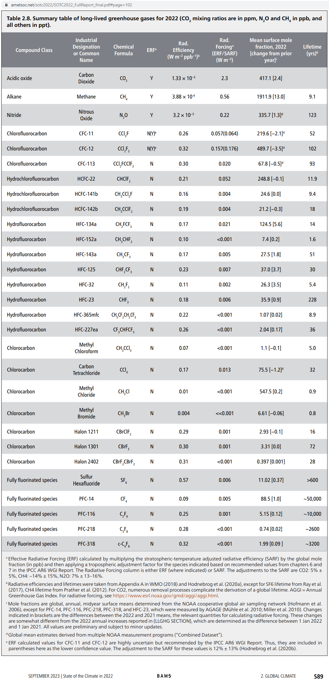
<br>
Re: <i>”CO2 dominates the forcing from these gasses until 1850 and was responsible for 83% of their forcing at that time.”</i>
“Until 1850?” What is interesting about forcings <i><b>before</b></i> 1850?
“83%” is a remarkably high, and remarkably precise, figure. Where does it come from?
From ice cores, our best estimate of <a href=”https://sealevel.info/co2.html”>CO2 level</a> in 1850 was just 285 ppmv, an increase of just 5 ppmv (just under 2%) since 1780.
CH4 (also <a href=”https://sealevel.info/EthCH498B.txt”>from ice cores</a>) in 1850 was about 790 ppbv, an increase of 60 ppbv (just over 8%) since 1780.
<a href=”https://climatemodels.uchicago.edu/modtran/”>MODTRAN</a> estimates that the 60 ppbv increase in CH4 generated about 2/3 as much radiative forcing as the 5 ppmv increase in CO2. That suggests your 83% figures is way too high.
<br>
Re: <i>”It is a reasonable assumption to say that, prior to 1850 the average climate sensitivity to all the NCGHGs combined was very close to CO2 sensitivity both historically and in 1850.”</i>
What does “climate sensitivity to all the NCGHGs combined” mean?
<br>
Re: <i>”The world will always have a strong GHG Effect while the sun continues to shine and that feedback to change for all concentrations of NCGHGs, including close to zero, will always be acting in a world with an existing strong GHG component.”</i>
That does not parse.
Radiative forcing from a change in CO2 level is closely proportional to the logarithm of the CO2 level.
Radiative forcing from CFCs is linearly proportional to the CFC levels.
Radiative forcing from CH4 is in-between.
<br>
Re: <i>”Reference Temperature (RT) is defined here as the base temperature attributed to a forcing before any … feedback has been applied. … For example, … CO2x2 … Reference Temperature (RT) of 1.2K. … In 1850 … and the total Reference Temperature for all the NCGHGs combined was 7.9K (IPCC). This is not contested.”</i>
That seems inconsistent. If RT for a doubling of CO2 is 1.2K, then how can RT in 1850, when GHGs had hardly been elevated at all, be 7.9K?
I think you’ve switched baselines, but it isn’t clear.
And what’s the source? “(IPCC)” is not a citation; you need a link or a footnote.
And what is your basis for saying, “This is not contested”?
<br>
Re: <i>”In 1850 the global temperature was 287.5K (NASA)”</i>
That seems a little high. (And “(NASA)” is not a citation; you need a link or a footnote.)
Note that there are at least two ways of defining an “average temperature” for the surface of the Earth. One is the obvious area-weighted average temperature, usually said to currently be about 288K. The other is a temperature which results in the actual average radiative emission strength; in other words, the fourth root of the area-weighted average of the fourth power of temperature in Kelvin. That second sort of “average” temperature is several degrees warmer. (The difference is sometimes called the “rectification effect.”)
<br>
As for “climate sensitivity” (to a doubling of CO2) here’s how you can estimate it:
Step 1. Note that globally averaged temperature has risen about 1.2 ±0.2°C since the (“pre-industrial”) Little Ice Age.
Step 2. Note that, even if we assume it was ALL caused by human activity (which is doubtful), at most 80% of it was due to the rise in CO2 (280 → 421 ppmv).
Step 3. Calculate that we’ve had log2(421/280) = 59% of the “radiative forcing” that we’d get from a doubling of CO2.
That means “practical sensitivity” = 1.2 × 0.8 / 0.59 = about 1.63°C/doubling.
If a portion of the warming since the “preindustrial” Little Ice Age was natural (as I suspect), then sensitivity is even less.
You can also do calculations like that using a shorter time period, with similar results. (Be sure to use endpoints during ENSO-neutral conditions.)
ECS is about 1.2× that, which makes it about 1.95°C/doubling.
That’s obviously not worrisome.
Oops, sorry, I forgot the HTML markup doesn’t work here. Trying again…
Translating…
“SGF” is the net amplification or attenuation from the action of all feedbacks. “SGF=1.09” means the net effect of all feedbacks is slightly positive (a slight amplification).
That’s probably a little bit low, but not wildly so.
But this essay needed some proofreading.
.
Re: “…Equilibrium Climate Sensitivity (ECS)… estimates … vary greatly.”
Here’s proof of that fact: The ECS estimates (warming from a doubling of CO2) baked into CMIP6 models vary from 1.83 to 5.64 °C!
The ERF estimates vary from 2.70 to 4.51 W/m². (The low end of that range is most consistent with measurements, and with calculations by Happer & van Wijngaarden.)
Ref:
https://github.com/mzelinka/cmip56_forcing_feedback_ecs/blob/master/CMIP6_ECS_ERF_fbks.txt
.
Re: “The Non-Condensing Green House Gasses (NCGHG) include CO2, CH4, N2O, CFC11, and CFC12.”
There are many others, too. Here’s a list from the AMS:
.
Re: “CO2 dominates the forcing from these gasses until 1850 and was responsible for 83% of their forcing at that time.”
“Until 1850?” What is interesting about forcings before 1850?
“83%” is a remarkably high, and remarkably precise, figure. Where does it come from?
From ice cores, our best estimate of CO2 level in 1850 was just 285 ppmv, an increase of just 5 ppmv (just under 2%) since 1780.
CH4 (also from ice cores) in 1850 was about 790 ppbv, an increase of 60 ppbv (just over 8%) since 1780.
MODTRAN estimates that the 60 ppbv increase in CH4 generated about 2/3 as much radiative forcing as the 5 ppmv increase in CO2. That suggests your 83% figures is way too high.
.
Re: “It is a reasonable assumption to say that, prior to 1850 the average climate sensitivity to all the NCGHGs combined was very close to CO2 sensitivity both historically and in 1850.”
What does “climate sensitivity to all the NCGHGs combined” mean?
.
Re: “The world will always have a strong GHG Effect while the sun continues to shine and that feedback to change for all concentrations of NCGHGs, including close to zero, will always be acting in a world with an existing strong GHG component.”
That does not parse.
Radiative forcing from a change in CO2 level is closely proportional to the logarithm of the CO2 level.
Radiative forcing from CFCs is linearly proportional to the CFC levels.
Radiative forcing from CH4 is in-between.
.
Re: “Reference Temperature (RT) is defined here as the base temperature attributed to a forcing before any … feedback has been applied. … For example, … CO2x2 … Reference Temperature (RT) of 1.2K. … In 1850 … and the total Reference Temperature for all the NCGHGs combined was 7.9K (IPCC). This is not contested.”
That seems inconsistent. If RT for a doubling of CO2 is 1.2K, then how can RT in 1850, when GHGs had hardly been elevated at all, be 7.9K?
I think you’ve switched baselines, but it isn’t clear.
And what’s the source? “(IPCC)” is not a citation; you need a link or a footnote.
And what is your basis for saying, “This is not contested”?
.
Re: “In 1850 the global temperature was 287.5K (NASA)”
That seems a little high. (And “(NASA)” is not a citation; you need a link or a footnote.)
Note that there are at least two ways of defining an “average temperature” for the surface of the Earth. One is the obvious area-weighted average temperature, usually said to currently be about 288K. The other is a temperature which results in the actual average radiative emission strength; in other words, the fourth root of the area-weighted average of the fourth power of temperature in Kelvin. That second sort of “average” temperature is several degrees warmer. (The difference is sometimes called the “rectification effect.”)
.
As for “climate sensitivity” (to a doubling of CO2) here’s how you can estimate it:
Step 1. Note that globally averaged temperature has risen about 1.2 ±0.2°C since the (“pre-industrial”) Little Ice Age.
Step 2. Note that, even if we assume it was ALL caused by human activity (which is doubtful), at most 80% of it was due to the rise in CO2 (280 → 421 ppmv).
Step 3. Calculate that we’ve had log2(421/280) = 59% of the “radiative forcing” that we’d get from a doubling of CO2.
That means “practical sensitivity” = 1.2 × 0.8 / 0.59 = about 1.63°C/doubling.
If a portion of the warming since the “preindustrial” Little Ice Age was natural (as I suspect), then sensitivity is even less.
You can also do calculations like that using a shorter time period, with similar results. (Be sure to use endpoints during ENSO-neutral conditions.)
ECS is about 1.2× that, which makes it about 1.95°C/doubling.
That’s obviously not worrisome.
There are many ways of estimating ECS: but the point of the head posting was to demonstrate that one cannot use feedback analysis to constrain it. Yet feedback analysis is the primary current method.
A little hard to follow but this seems to take the wind out of the IPCC sails.
This analysis seems to be completely flawed since it confuses temperatures changes with absolute temperatures. It starts by defining:
“Reference Temperature (RT) is defined here as the base temperature attributed to a forcing before any atmospheric or ocean feedback has been applied. For example, the Reference Temperature for CO2x2 is agreed at 1.2C (Hansen ’84).”
now clearly the Reference Temperature is a temperature difference since the figure of 1.2C is the amount by which the average temperature will increase. Similar the Equilibrium temperature also refers to a temperature difference relatively to the current temperature.
Thus the definition of the system gain factor only makes sense as the ratio of two temperature differences relative to today’s (or the 1850’s) temperature. This is evident in Eq .1 for “A”
But then in Eq. 2 there is a completely different definition of “A” It now refers to the
ratio of the blackbody emission temperature and the earth’s actual temperature. And since
this definition is different from the definition used in Eq. 1 it isn’t logical to combine the two
and it should come as no surprise that the result doesn’t make sense.
There is no way to calculate the effect of CO2 by comparing temperatures at two points in time.
That is especially true if the tart point is in the 1800s where the global average temperature statistic is based mainly on infilling (guesses) and few measurements. Questionable measurements of ocean temperatures.
There are a large number of climate change variables, global, regional and local, that affected the climate in the past 150+ years.
To know the effect of CO2, you would have to know the effect of perhaps 10 different natural and manmade climate change variables.
Such knowledge does not exist.
Therefore the effect of CO2 in the atmosphere can only be estimated by isolating CO2 in a laboratory and assuming those measurements apply to CO2 in the atmosphere.
The author of this article uses the temperature change between two points in time to estimate the effect of CO2 in the atmosphere.
I have just explained why that is incompetent science and can not improve on estimates of the atmospheric effects of CO2 from lab spectroscopy.
Mr Greene is attempting to repeal the laws of calculus. To find ECS, one take two points – such as the 1850 equilibrium and the predicted equilibrium following a forcing equivalent to that from doubling CO2 compared with 1850, and the slope of the line between those two points – an approximation to the desired derivative – is the ratio of the differences between the two equilibrium temperatures and the two reference temperatures. That works out at ECS / RCS. From those facts, one can in reality deduce quite a lot about the influence of CO2 on temperature – chiefly, that it is very likely to be minimal.
As for complicating the matter with other climate variables, of which there are thousands, climatology keeps all of them constant other than the variable that is of interest. If Mr Greene does not like this standard technique in physics, let him address his whining to IPCC and not bore us with his scientific ignorance here.
If Mr Green is unaware of the method of approximating the slope of a function at a point of interest by taking the slope of the line that connects two points close by, then he should not state that this is “incompetent science”. It is Calculus 101, which, evidently, Mr Greene has not studied.
He has a regrettable propensity to condemn as unscientific anything that he does not understand. Since he does not understand anything, everything to him is unscientific. He is not contributing anything valuable here and, on behalf of the community here, I must ask him to desist until he has learned some mathematics – and some manners.
It would be great if the author defined what he thinks the word “feedback” means. Coming from an electronics/control system background it seems to me that it is being misused or misunderstood.
Feedback in a dynamical system (i.e., in a system that changes its state over time) is an additional, indirect signal responding to, and proportional to, a direct or reference signal, so that the sum of the reference signal and the feedback-response signal is the output signal. In the climate, temperature feedbacks respond to the entire reference temperature obtaining at a given moment, and respond proportionately to the magnitudes of the components in that reference temperature. A positive feedback amplifies the reference signal; a negative feedback attenuates it.
Feedback intensity in the climate is denominated in Watts per square meter per Kelvin of the reference temperature.
The feedback factor, the operant in the feedback loop, is the unitless ratio of feedback intensity to the 3.2 W/m^2/K Planck response (itself the first derivative of the Stefan-Boltzmann equation with reference to net incoming radiative flux density at the top of the atmosphere and mean industrial-era surface temperature).
The system-gain factor, the ratio of the equilibrium or output temperature to the reference or input temperature, is equal to 1 minus the reciprocal of the system-gain factor.
The unit feedback response, the ratio of the feedback response to the reference temperature, is equal to the system-gain factor minus 1.
The feedback response, in Kelvin, is the difference between the equilibrium temperature and the reference temperature.
The reference is many times called the “set point”. Just like the thermostat in your house is “set” to a reference temperature. The output of the thermostat is the feedback response, the set temp vs the output temp (i.e. the temp in the house). For the thermostat it’s a pretty simple feedback response, furnace on or furnace off. But that feedback response can get *very* complicated for other processes.
I agree, Red! Here’s how it should be defined:
https://sealevel.info/feedbacks.html
If CO2 is sensitive to IR so that warming takes place why is there not two columns in the specific heat table? One for energy with IR and one column for energy without IR.
Q = Cp * m * dT does not care about the type of energy only the amount.
Because dT is frequency dependent. If the “mass” doesn’t intercept the energy dT will be zero. CO2 as the “mass” only intercepts energy at certainty frequencies, that being in the IR range. And it doesn’t even intercept all IR frequencies, just a narrow bandwidth.
I asked about the missing ozone in the calculation, and found that there is a reference temperature of about 3,5 degree C. This is dependent of the O2 level in the atmosphere. It will possibly change a little bit with change i solar radiation, especially UV radiation. And also a minimal influence from temperature level.
Effects of Ozone Levels on Climate Through Earth History
Russell Deitrick1 and Colin Goldblatt1 1School of Earth and Ocean Sciences, University of Victoria, Victoria, British Columbia, Canada
Molecular oxygen in our atmosphere has increased from less than a part per million in the Archean Eon, to a fraction of a percent in the Proterozoic, and finally to modern levels during the Phanerozoic. While oxygen itself has only minor radiative and climatic effects, the accompanying ozone has important consequences for Earth climate. Using the Community Earth System Model (CESM), a 3-D general circulation model, we test the effects of various levels of ozone on Earth’s climate. 5 When CO2 is held constant, the global mean surface temperature decreases with decreasing ozone, with a maximum drop of ∼ 3.5 K at near total ozone removal. By supplementing our GCM results with 1-D radiative flux calculations, we are able to test which changes to the atmosphere are responsible for this temperature change. We find that the surface temperature change is caused mostly by the stratosphere being much colder when ozone is absent; this makes it drier, substantially weakening the greenhouse effect. We also examine the effect of the structure of the upper troposphere and lower stratosphere on the formation 10 of clouds, and on the global circulation. At low ozone, both high and low clouds become more abundant, due to changes in the tropospheric stability. These generate opposing short-wave and long-wave radiative forcings that are nearly equal. The Hadley circulation and tropospheric jet streams are strengthened, while the stratospheric polar jets are weakened, the latter being a direct consequence of the change in stratospheric temperatures. This work identifies the major climatic impacts of ozone, an important piece of the evolution of Earth’s atmosphere.
And then the clouds. There will be some variations, and some change with warming climate?
“Reference temperature” year 2000 ?? -5 degrees C.
http://www-das.uwyo.edu/~geerts/cwx/notes/chap09/rossow.html
Clouds cool the Earth by reflecting incoming sunlight. The tiny drops or ice particles in clouds scatter between 20 and 90 percent of the sunlight that strikes them, giving them their bright, white appearance. From space, clouds look bright whereas large bodies of water look dark. A cloud-free Earth would absorb nearly 20 percent more heat from the sun than the present Earth does. To be in radiation balance Earth would have to be warmer by about 12�C. Clouds cool the planet by reflecting sunlight back into space, much as they chill a summer’s day at the beach.Clouds warm the Earth by absorbing infrared radiation emitted from the surface and reradiating it back down. The process traps heat like a blanket and slows the rate at which the surface can cool. The blanketing effect warms Earth’s surface by some 7�C.Thus the net effect of clouds on the climate is to cool the surface by about 5�C, at least under the current global distribution of clouds. Clouds reflect about 50 W m-2 of solar radiation up into space, and radiate about 30 W m-2 down to the ground, so the net effect is 20 W m-2 cooling on average.