Guest post by Ed Zuiderwijk
Yes, you read it correctly. And no, it’s not about the good citizens of Poland. Why are the poles warm and the tropics cold, and compared to what? An equivalent question is: what determines the difference in temperature between tropics and poles, and can we understand why that difference has the magnitude it has on the real planet Earth? Just for the record, there is not a single climate simulation model that tells us what that difference should be, let alone why its magnitude is what it is; it is one of the boundary conditions at the start of a climate ‘run’.
One of the delights of discussions with climate scientists is that it gives you an insight in their way of thinking. For instance, take the often posited: ‘one should look at the big picture’. What many climate scientists mean by that is considering the latest super-duper ocean-atmosphere coupled models with line-by-line radiative transfer codes and what not more. Without that, the claim is, you cannot understand how the climate system works. Curiously, to a physicist such as yours truly ‘looking at the big picture’ means precisely the opposite: stripping down the system under consideration to its knuckle-bare essentials and glean insights about its inner workings from the underlaying physics without being distracted by detail.
So what’s here the big picture? In its simplest form the Earth is a heat-transfer system in non-equilibrium (but in a steady state) where heat (predominantly) enters in the equatorial regions and heat is (predominantly) lost at the poles. Inside, heat is transported from the tropics to the poles by atmospheric and oceanic currents, cooling the tropics and warming the polar regions. Without such transport the local temperature would have been determined by the balance between insolation and radiative losses only, which would make the tropics warmer than they are and the poles colder. The tropics are cooler than they would have been without that transport, while the polar regions are warmer. Hence, cold tropics and warm poles.
Now here is the conundrum: the heat transfer between tropics and polar regions is determined by their temperature difference. The larger it is, the bigger the heat flow. But the heat transfer reduces that temperature difference and thus acts against its own causation. For instance consider the limiting case of a very large heat flow in which the heat transfer is practically instantaneous. As a result the poles would have the same temperature as the tropics, but then there can be no heat flow at all, because that is driven by a temperature difference. Thus we have a contradiction. Starting from the converse situation of no heat flow is also untenable because the large temperature difference will induce a heat flow. Yet, there is a heat flow, which therefore must be consistent with the temperature difference it causes. A smaller temperature difference will not be possible, because that would decrease the heat flow and thus increase that difference again; and a larger temperature difference would increase the heat flow, thus decreasing it. This suggests strongly that the atmosphere as a whole settles in a state where the temperature difference between tropics and poles is minimal while concurrently the heat flow it causes between them is maximal. We can use this insight to calculate its magnitude by applying the principle of Maximum Entropy Production MEP, a working hypothesis in non-equilibrium thermodynamics which has increasing support in observations (see Kleidon for an excellent introduction, refs 1, 2).
The MEP principle states that a system far from (thermodynamic) equilibrium will adapt to a steady state in which energy is dissipated and entropy produced at the maximum possible rate. Notice that ‘maximum entropy production’ is something completely different from ‘maximum entropy’. The latter relates to a closed system in thermodynamic equilibrium. Here we are dealing with an open system not in thermodynamic equilibrium but in a steady state of non-equilibrium.
I’m afraid I’ll have to introduce here some formulae. What I’ll do is give the basic equation and it’s solution here, while putting how you can find that solution in an appendix for the aficionados. Those familiar with thermodynamics will know this expression for the production, that is the change, dS of entropy S by a change of heat content dQ at temperature T:

From this follows directly the expression for the entropy production by a heat flow Q between the equatorial regions at temperature Te and the poles at Tp:

The heat leaves the equatorial regions at temperature Te, hence the minus sign, and arrives at the poles at temperature Tp. Maximising S is akin to finding the optimum combination of Q and Te -Tp. The solution of this equation is rather straightforward (see the appendix). The actual difference Te -Tp comes out at very nearly half the difference there would have been without energy flow. Half, hence not 0.3 or 0.7 times.
Let’s test this result against models and observations. It appears to be well established – from calculations with standard atmospheric models – that without the heat transfer the equatorial regions would be about 15 degrees warmer and the poles about 25 degrees colder (Centigrade, ref 3). I take these estimates at face value; they imply an asymmetry β = 0.25 for which 1 – 2α ~ 0.51 (re: appendix). Then the prediction is that the temperature difference between tropics and the poles with the heat transfer is about 41 degrees (being (15 + 25) × 0.51∕0.49) while the difference without would be about 80 degrees. The table lists some real observations.
| Region | Temperature range | T mean | Notes |
| Arctic | -32 +6 | -13 | Danish Arctic Survey (> 80oL) |
| Antarctic | -32 -17 | -28 | Byrd Station |
| Tropics | 21 29 | 24 |
Observed Polar and Equatorial Temperatures (Centigrade)
For the Antarctic I used data from the Byrd station because it was located on a plateau and therefore presumably less affected by possible shielding by mountains. The averaged polar temperature appears to be about -21C. For the tropics the lower end of the range corresponds predominantly to oceanic data and should therefore have a larger weight in the mean, here taken as 24C. Thus the observed temperature difference between polar and equatorial regions comes out at about 45 degrees, against a prediction of 41 degrees. Not bad for such a basic model.
It may be a simple model but the MEP principle has an important implication. Maximisation of entropy production for steady-state conditions implies a strong negative feedback to perturbations (see Kleidon). Any perturbation will lead to a decrease in S, by definition, and the system will adjust trying to optimise it again. One such perturbation in climate models is well-known and long established and widely accepted as a valid concept: the ‘polar amplification’. It says that in a warming atmosphere the polar regions warm faster than the equatorial regions; hence that Te – Tp decreases. However, it is also one of the oddest concepts to be found in climate modelling because it has no limiting condition: nowhere in the literature does it say something like ‘under this and that conditions, at this level of warming, the polar amplification will stop’. This could lead to an absurdity: should the atmosphere get hot enough the temperature difference between equator and pole would disappear completely or even change sign. Therefore there must be conditions when the amplification does not happen anymore. Why is this important? If there is such a mechanism which kicks in under certain circumstances then one has to explain why it does not work at this very moment and that could be embarrassing. Whatever the case may be, from the foregoing it should be obvious that the concept of polar amplification is in fact rather questionable: the decreased difference of polar and equatorial temperatures reduces the heat flow to the polar regions which would result in a cooling. A realistic climate model should behave as the underlaying physics dictates. It can be deduced, therefore, that such a feedback is absent in current climate models and that consequently the whole concept could be an artefact of an incomplete model. [You read it here first.]
But, as luck would have it, the Arctic has warmed over the past 3 or 4 decades. That would prove the polar amplification concept, wouldn’t it? Well, that warming may be the case in the Arctic, but it should also apply to the Antarctic at the same time, but there the concept appears to fail the test against observations (ref 4).
So what may be going on then in the Arctic? If I’m allowed, I put here my two cents worth on the subject. To me, the key is in the fact that there are two poles. It would be extraordinary if at all times precisely the same fraction of equatorial heat would be partitioned to each pole. The transfer mechanisms, atmospheric and in particular ocean currents, are inherently chaotic systems, prone to switch from one particular quasi-stable flow pattern to another. For ocean currents we know this behaviour as the Pacific Decadal Oscillation, the Atlantic Multi-decadal Oscillation, the Indian Ocean Dipole and the like. The timescale for such changes is many decades, from 3 for the PDO, to 6-8 for the AMO, because there is an enormous mass and momentum of moving water involved and water is an incompressible fluid which means that the change occurs over the whole flow pattern simultaneously. Therefore it is to be expected that the partitioning of heat to the north and south is subject to changes on a timescale of decades in an erratic seesaw fashion. We happen to live in a time when the northern hemisphere gets a bit more than its fair share of the heat; in a few decades it may be completely different. To disentangle such changes from a possible underlaying long-term warming trend will require data over a much longer timespan then we have now.
References:
(1) Axel Kleidon (2009): ”Non-equilibrium thermodynamics and maximum entropy production in the Earth system”, https://link.springer.com/article/10.1007/s00114-009-0509-x
(2) A Kleidon, R D Lorenz (editors) ”Non-equilibrium thermodynamics and the production of entropy” (2005) Springer, ISBN 978-3-540-22495
(3) e.g. http://earthguide.ucsd.edu/virtualmuseum/virtualmuseum/EarthsClimateMachine.shtml
(4) e.g. https://wattsupwiththat.com/2019/04/10/the-curious-case-of-the-southern-ocean-and-the-peer-reviewed-journal/
Solving the EP equation
The entropy production S for a heat flow Q between the equatorial regions of temperature Te and the polar regions of temperature Tp is given by:

The MEP hypothesis is that the atmospheric system tends to maximise S. This optimum can be found analytically as follows. Introduce Θe and Θp, the temperatures of the equatorial and polar regions respectively if there were no heat transport. That is, Θe and Θp stand for the radiative equilibrium temperatures of those regions. The actual temperatures (Te and Tp) are different because of the heat transport. Hence define ΔTe = Θe – Te and ΔTp = Tp – Θp. Let’s for the moment assume that they are both equal and equal to a fraction α of the range Θe – Θp:

Notice that the difference Te – Tp equals:

Obviously for α = 0 there is no heat transfer, hence S = 0, while for α = 0.5 we have Te equal to Tp and thus no entropy production either. In between these extremes the heat flux Q is somehow proportional to ΔTe, the larger the drop in temperature of the equatorial region, the larger the heat loss from it and one can assume the relation to be (close to) linear. This gives us an expression for S in terms of ΔT, hence as function of α :

The maximum of S in the range [0.0 – 0.5] is straightforwardly found with basic calculus techniques – you need to solve a cubic equation in α – and turns out to be almost exactly at α = 0.25. Alternatively, one could use the R analysis package, encode the function for S, find the maximum with Newton’s method and get a figure as a bonus.

The upshot of all this is that the MEP temperature difference Te -Tp is very nearly half the difference Θe – Θp which we would have had in the absence of any heat flow.
Let’s now revisit ΔTe and ΔTp. Adopting equality of ΔTe and ΔTp means assuming that for every degree drop in temperature of the equatorial regions the polar temperature rises by one degree. This is not very realistic; quite likely the polar temperature rises more because of area and heat capacity differences. We can include such an imbalance by slightly modifying the definitions of ΔTe and ΔTp and introduce an asymmetry parameter β:

With a value of β = 0.25, for instance, this would mean that for every 3 degrees drop in equatorial temperature the poles would gain 5 degrees. Notice that the difference Te – Tp remains as given earlier. Repeating the foregoing exercise for a range of β values presents us with an interesting result: the corresponding α values are practically unchanged: for β = 0 the maximum is at α = 0.2487, for β = 0.25 at 0.2441 and β = 0.33 at 0.2427. This means that irrespective of a possible asymmetry between equator and polar regions the temperature difference between the two remains firmly at about half the difference Θe – Θp, but that the centre of the range shifts according to the value of β.
The only available process to achieve the observed outcome is variability in the rate and distribution of convective overturning.
Stephen
it’s mainly CLOUDS that control the Earth’s heat balance by reflection of sunshine, in turn controlled by evaporation rates off the ocean’s surface, but also water vapor content in the lower troposphere that absorbs IR, opposing the cloud SW reflection.
Clouds do modify the system but convection then changes to keep the system stable.
Increased convection causes more clouds in the area that’s hot (air rising) and fewer clouds in the area that’s cold (air sinking).
So lets take a patch of ocean, say around Hawaii, water temp 15C,,and for sake of having a real size to talk about, let’s say 10 M x 10 M….Solar input…say 1000 W/sq.M….heat goes 90% into evaporating and 10% into heating the water…In an hour the .9 KW/sq.M will generate .9/2.26×100 sqM = 40 kg of water vapor….Air weighs 1.225 Kg/cu.M and is saturated at .0128 Kg/cu.M, so in 1 hour there is 3125 cu.M of water saturated air that is going to be a cloud if it cools a bit as it convects upward. That’s a big volume of cloud thats not going to stay over the original 10x 10 plot…will probably reflect sunlight from 3 times as area as the originally considered area. I could have made it 10 Km by 10 Km but everyone would be lost in the numbers.
Clouds are a very large feedback on surface temperature, despite climatologists’ apparent inability to do basic evaporation pan calculations done at thousands of agricultural weather stations worldwide and extrapolating them to ocean sized areas.
This water is evaporating off the surface then wouldn’t the underlying water be cooling off instead of heating up? And, what percent of the energy is reflected back to space off the surface, not heating anything?
Reflection wins by a long margin once conditions enable cloudburst. The reflective power of clouds increases rapidly above tropical sea surface as the temperature rises above 26C. So much that the SST can never exceed 32C in open ocean.
For the back of napkin numbers I used, we are putting heat in at a sufficient rate that the top couple of mm is the warmest. When the sun goes down and the wind has a relative humidity less than 100%, then your thought is correct. In the example, I used 1000 W/sq.M which is approximately overhead sunshine. The albedo of the ocean about .06 under such conditions, so only 6% of the incoming SW is reflected. At low light incidence angles, say nearing sunset, as one would expect, the radiation is mostly reflected, unless the horizon is “wavy”…. but the cosine of the zenith angle is so small, heat absorbed by the surface becomes less than heat absorbed by the long path through the atmosphere. Hope this answers your questions.
And The Albedo difference between open ocean .06 (absorbing 94% of incident heat) and the albedo of the clouds, up to 0.9, and the generation of additional cloud area reflecting sunshine back into outer space is what controls the planets temperature. All Clausius Clapeyron equation. CO2 only has some minor effect on the elevation that clouds form at due to increase C02 radiation of heat to outer space at top of troposphere, and increased absorption lower in the troposphere where CO2 and water content are about equal. Water content at top of troposphere is only 20 ppm and C02 is 400 ppm.
Before evaporation can increase, water first has to warm up. Evaporation limits how much the temperature of the water can rise, it can’t prevent the temperature from rising.
Mark, I fear that isn’t true. Over most of its range, evaporation is a linear function of wind speed, such that if wind speed doubles, evaporation doubles.
And of course, in a cyclone, wind speeds are through the roof … literally.
My best to you,
w.
And Willis, a linear function of (100% RH – %RH) of the wind, which is also the same linearity as Pw x (100%-%RH)….Where Pw is the vapor pressure of water that increases about 7% per degree of water temp….for those that like equations that explain tropical thunderstorms….
The atmosphere changes gear once the water column reaches 30mm. The attached image from the Convective Working Group shows how strongly TPW and convective instability are related.
Cloudburst is a consequence of instability and produces the highly reflective high level cloud that limits the SST to 32C. Cloudburst is the thermostat of the tropical oceans.
At some point I stopped reading as
I was reminded of Hiawatha’s mittens:
He killed the noble Mudjokivis.
Of the skin he made him mittens,
Made them with the fur side inside,
Made them with the skin side outside.
He, to get the warm side inside,
Put the inside skin side outside;
He, to get the cold side outside,
Put the warm side fur side inside.
That ’s why he put the fur side inside,
Why he put the skin side outside,
Why he turned them inside outside.
This dude have fur on ‘is memba?
WUWT?
Inside, heat is transported from the tropics
to the poles by atmospheric ocean currents,
cooling tropics and warming polar regions.
Hamms the beer refreshing
Isn’t weather caused by the temperature difference between the equator and the poles?
Globally, cold, dense air over the poles sinks, while hot, light air over the equator rises, since nature abhors a vacuum the net effect of the flow from one to the other we call wind. The coriolis effect causes circulation producing weather systems.
Surely, the potential energy in the atmosphere is reducing due to that falling temperature difference?
Arguing otherwise would appear to be non physical.
Total potential energy stays the same. If the average surface temperature rises then convective overturning runs faster so as to maintain energy output to space from the surface at the correct rate to retain hydrostatic equilibrium.
The opposite if average surface temperature falls.
You have to consider both the surface horizontal flows and the convective up and down flows together. Between the two sets of energy flows any heating or cooling from radiative imbalances is neutralised.
It is all about the mechanical process of bulk mass movement within a gravity field.
There are a series of convective ‘cells’ simplistically identified as three sets of cells in the atmosphere the Hadley cells that incorporate the heat rising from the equator and then the air descending down at mid latitudes, these abut the Ferrel cells from mid-latitudes and they abut the polar cells. The atmosphere will move very fast in response to heating; but in comparison to the oceans the atmospheric circulation carries very very little energy. However, the rising convection at the equator causes towering dense cumulonimbus clouds at the Inter Tropical Convergence Zone, which not only convect heat away from the surface returning cool rain, but also rapidly raise the earth’s albedo at the equator reducing the energy input from the Sun. This energy loss, reflection and feedback effect was not part of the post but is very important as it significantly reduces energy input to the system.
The Thermo Haline Current (THC) is very slow not only carrying huge amounts of energy dwarfing that in the entire atmosphere. The THC also sequesters that energy from effects on the weather systems when flowing well below the surface. Whereas solar heating effects on the atmosphere are apparent in hours, ocean currents are far slower, with the complete THC (it is said) lasting hundreds to thousands of years.
While the atmospheric and ocean circulations could be considered under one equation for maximizing entropy, the temporal and energy differences are so large that one equation may be too simplistic. The warming poles may be warm because of something happening nearly a century ago from the ocean circulation or a few days ago from the atmosphere circulation. This could lead to a chaotic mismatch in timing of the feedback response or perhaps it should be considered that the slower larger energy transport of the THC has a damping effect on the rapid more variable atmospheric response.
Have a look at today’s photos from EPIC
https://epic.gsfc.nasa.gov/
From this you can glean that Hadley, Farrel, and Polar cells are a teaching construct by academia, while real weather systems are more affected by Coriolis forces.
Those three cells are real but vary greatly over time as the Coriolis forces jumble up the latitudinal energy flows around the Earth between the lit and unlit sides.
I agree the simplified diagrams are difficult to find in the real world. However, the dry descending air from the Hadley and Ferrel cells leads to the bands of deserts around their lattitude. The jet streams caused by the geostrophic and Coriolis forces as they pass ‘slower’ moving air will be pulled into loops Rossby waves that may themselves slowly move around or be blocked into position by ‘omega’ highs and the entire looping pattern held in place for a while. On average though the pattern of Ferrel cells and Hadley cells is there. This year the line of the sub-tropical jet in the Northern hemisphere is a lot more southerly than normal leading to snows in Morocco, Algeria and the Sahara and the Nor’Easters being experienced now in the USA with fronts extending from Canada down to the southern Caribbean.
The amount of energy even if you only consider the convective effects and latent heat of water on condensing, freezing and melting -is huge. It is still dwarfed by the energy in the oceans but the THC moves extremely slowly.
Will cooling in the tropics cause warming of the poles and as a result increase the heat loss to space?
If you assume the total energy in the atmosphere stays the same, then warming somewhere means there is cooling somewhere else. If the energy content, thus temperature, is generally increasing, and there is good heat transport from tropics to poles, then the the poles will warm more than the tropics because they are a lot smaller in area, and a lower T^4 for IR radiation to space.
I know that maximum entropy production was quite a popular idea a couple of decades ago, but there are a number of problems with it. First, there is no underlying general principle. The idea of maximum entropy has underlying it the perfectly reasonable principle that systems evolve toward more likely configurations. Maximum entropy production has nothing similar.
Second, Prigogine has shown that within certain assumptions linear constitutive relationships (Fourier’s law of heat transport is just such a relationship) there is a principle of <i><b>minimum</b></i> entropy production.
Third, here is an observational counterexample. The transition from nucleate to film boiling (boiling crisis) looks to me like it defies a maximum entropy production principle if there is such a thing.
Fourth, you have two formulae for S which have different units. This can’t be.
How far is the Atmosphere/Ocean system from equilibrium? Do linear constitutive apply to it, or does it call for higher order terms?
I believe that entropy balance can answer many interesting questions about hypothetical climate and weather situations, but is there a single example of anyone using it? People check that weather and climate models adhere to the first law of thermodynamics, but I doubt they check to see that these models adhere to an entropy balance.
I do have the impression that MEP is more general than the ordinary statistical physics as it instead of the microcanonical ensemble studies the phase space processes which mage it handle even nonlinear phenomena. Prigogines and Onsagers ideas and solutions are based on linearized approximations. Please read the theory and check if I am wrong? In the 1990-s the concept has successfully been used to derive bounds for the climate on any planet.
Quote:
“”People check that weather and climate models adhere to the first law of thermodynamics, but I doubt they check to see that these models adhere to an entropy balance.””
Maybe they should check the Entropy and that it is always increasing.
If not and they find Entropy is decreasing, then they thus have heat energy moving UP a thermal gradient.
Patent garbage.
And as I understand it the very crux of the GHGE, that energy from anywhere in the atmosphere returns to Earth’s surface and adds to the energy content of whatever it lands upon. Land, ocean, forest, city whatever whatever
This ‘downwelling’ heat energy CAN NOT do that – the sky is at all points is colder than the surface below it (Lapse Rate tells you that).
No matter how much energy you think comes down from the atmosphere and or the Green House Gases within it, that energy will have no effect on the temperature of the surface.
Stefan told us that.
Chatelier told us that.
Carnot told us that, lest we build a heat-engine with negative efficiency
The Cooling Universe tells us that
Probably Joule also
……all of which are explanations of Entropy
Is THAT the misunderstanding, which I’ve seen repeated here many times?
Not least Willis in his various essays.
They state that The Energy, once radiated, cannot ‘know’ where it is going and is thus *compelled* to be absorbed by the first thing it impinges upon ##
No no no
If it hits an object warmer than where it set off from, it is reflected, scattered or maybe goes straight on through.
It does not contravene the 1st Law – the energy just keeps on bouncing around until it *does* hit something colder than where it started – and ‘does its bit’ to try warm that object
Thus I’d assert that a check on Entropy inside climate models would be a good idea.
Just Entropy, not its production, acceleration or anything more exotic.
## Mythical ‘Perfect Black Bodies’ are imagined to make that so. There can not and is not any such thing. It would have a temperature of zero Kelvin yet even the emptiness of intergalactic space has a temp of 4 Kelvin.
There are NO Black Objects anywhere
“If it hits an object warmer than where it set off from, it is reflected, scattered or maybe goes straight on through.”
That is just about the most absurd statement on physics I have ever seen. Do you have any good theory about how the photon remembers the temperature when it was emitted and how it checks the temperature of the object it hits before it decides what to do?
The energy of the photon is due in part to the temperature of the emitting atom/molecule.
However whether or not the photon is absorbed has nothing to do with the temperature of the target atom/molecule. It depends entirely on whether or not the target has an open energy band that matches the energy of the photon.
I couldn’t agree more.
The energy of a photon is is related to the resulting frequency (wavelength) of the EM wave. E=hc/λ. But, that is only part of the process of determining the total energy emitted. If you go no further, you’ll be assuming that a molecule only emits a very, very small amount of energy (one photon) when it loses it vibration, rotation, or translation.
This is the guy who believes that deserts are not caused by a lack of water, but by repeated forest fires.
Perhaps a brief review is called for. Energy in radiation is carried by Electro Magnetic waves (EM waves). EM waves can have varying power levels, ala, radio stations, or in other words more or less energy. That energy determines the value of the E and H fields in the wave.
The frequency of the EM wave is determined by the originating molecule. For IR from CO2, the predominate wavelength is 15 um. When an EM wave encounters a molecule, if it has the correct frequency, the molecule can absorb energy in ‘quanta’ amounts, or photons if you will. And if, the EM wave has enough power it can excite the molecule to higher levels. The problem is that the more excited a molecule becomes, the faster it will also re-emit that energy.
Look up how to convert watts to photons per second.
EM waves also obey the inverse square law, just like gravity. That means the further it travels, the less the power that can be drawn from the wave. Think about that and how it applies to back radiation. That is, if an EM wave is generated by a molecule of earth and travels 1 meter to a CO2 molecule, then travels back the 1 meter how much energy is lost?
Lastly, photons are not bullets being shot out of molecules traveling until they encounter a target. EM waves from molecules are spherical because a molecule is pretty much the definition of a point source.
Does any of this help?
Photons are not affected by the inverse square laws. A photon can travel millions of light years without losing any energy at all.
The inverse square law impacts how many photons are found per unit area. The further from the source, the more disperse the photons.
How much energy is lost when a photon travels a meter then back again? None.
Photons are both waves and particles at the same time. When talking about energy being transmitted between two molecules, thinking of the photon as a bullet is not an invalid analogy.
Photons don’t travel through space by themselves, therefore they can’t be considered “bullets”. EM waves are the energy carrying mechanism that transports energy. EM waves have both frequency and power. That is why a 500 watt microwave doesn’t heat as fast as a 1200 watt one.
The energy in an individual photon is not affected by distance because that is determined by the frequency, however the number of photons available in a given area does vary by the inverse square law because the available power is dispersed as the wave expands.
Remember it is EM waves that have a duality that lets them act like a particle in certain situations. Photons are not particles that act like waves at certain times.
Here is a url of a book that explains some of this. This is from page 203 of the book. “This relation gives us a way to find the magnitude of the vector potential A0 if we know the power carried per unit area by the electromagnetic wave. Since energy in electromagnetic waves is carried in quantum packets (photons) of individual energy ~!, the number of photons that cross unit area per unit time is then given by (equation)”
Physics for Semiconductors (cornell.edu)
It is important that this process be understood in order to evaluate what happens with CO2. Think about this, is the earth radiating more 15 um EM waves today than 100, 1000, 10000, or 100000 years ago? Shouldn’t more CO2 be reducing/increasing the amount of 15 um seen at the TOA? Have you seen any studies that evaluate this? I haven’t. All I ever see are the same old, tired black body diagrams that never change what happens at 15 um. If that is truly the case, then CO2 has been saturated for a long time and what we do really doesn’t matter.
“Perfect blackbody…zero Kelvin”. You misunderstand what a “blackbody” is. A perfect blackbody (which is a theoretical object) at a given temperature emits according to the Planck formula. Real objects at non-zero temperatures emit similarly, with the differences depending on their emissivity characteristics.
One can get pretty close to the ideal curve over some limited part of the spectrum by choosing the right coating.
“No no no.” Yes, yes, yes. A photon, which is what carries thermal energy away from the planet, is completely characterized by its wavelength. It will be absorbed or reflected by any matter that it hits, probabilistically, according only to the emissivity of the object that it hits.
That object will be simultaneously emitting energy according to its temperature and emissivity. Whether that object – whether it be an atom of gas or a solid – gains energy or not can only be determined in the long term by whether it absorbs or emits more energy (and, of course, whether it also is receiving or losing thermal energy through conduction).
As I remember from Dewar and Ozawa, 2003, your statements one, two and three are incorrect. MEP is a first nonlinear generalized step in the direction of understanding turbulence. Instead of working with billiard balls like classical thermodynamics, you work with their paths. The theory is complicated but the benefits are huge. Prigogine was working at the lowest energy level prior to full turbulence while MEP takes the step out. There are critique of MEP but many of these writers merely show their ignorance of the topic.
But, but but…..CO2….. [/snark]. So, what would be the range of (1-2*alpha) and the corresponding delta temps between the tropics and polar areas for the entropy production at or above 98% of maximum? Given the time lags due to all the various transport mechanisms, I could see there being some “rattling around” those maximum delta temp values. How does that range compare to observed temperature variations? How much kinetic energy is there in the moving mass of the ocean currents, and how does that kinetic energy change when the AMO and PDO and other currents flip through their various states? How long would it take for insolation to impart that amount of extra kinetic energy into the systems at the higher energy state vs the lower? How long would it take for those currents to die down if the energy input were eliminated at the flip of a switch (e.g. the inertia of those transport mechanisms)? Are there “emergent phenomena” (like tropical afternoon thunderstorms) in those currents where they are in one state, doing their energy transport from the warm tropics to the cool poles until such time as they transport too much (or too little) energy due to the mass & inertia involved, allowing a buildup (or deficit) in energy in the warm (or cool) which causes the flip in state?
I know enough about aircraft structure to know the non-linear effects when permanent deformations start near the breaking point (and load starts shifting from one piece to another) are complex enough that no matter how sophisticated the structural modeling is, and how well understood linear elastic and non-linear plastic deformation of structure is, the regulators require a physical test of all new airplanes to prove the structure and analysis and modeling, unequivocally. The engineering challenge of getting this analysis right is trivial compared to the complexity of the climate. As well understood as aluminum structures are, engineering still can’t get it right 100% of the time (2 major western built transport category airplanes failed their proof tests and had to have the structure reinforced as a result – one by a couple percent, another by about 15%). And yet, these AGW climate clowns have the hubris and arrogance to tell us they understand it all from tap, tap, tapping away at their keyboards (and that all is due to a trace gas that is 0.3% of the total atmosphere).
You are over-estimating, CO2 is currently 0.04% of the atmosphere.
CO@ur momisugly is about 0.04%. Which gas isj0.3%?
Of course there is a big difference between the poles. The ocean all around Antarctica and the “West wind belt” strongly impedes heat transport to the South Polar region, and has done so for c. 35 million years now.
Also there is a difference between heat and energy (which is the really relevant quantity). A similar amount of energy will cause a much larger temperature change in cold, dry arctic air than in warm, wet tropical air.
Thanks Charles for some refreshingly real climate science.
One of the several pillars of climate dynamics that the CO2 church are trying to destroy by ignoring is the fact that the continental configuration i.e. the world map makes a difference to climate.
Nowadays your average climate novitiate-postulant submitting papers for publication will diligently ignore any cause of present or past climate change except CO2. So in any paper on interpretation of past climate proxies, be it thousands or hundreds of millions of years ago, the only driver of global temperature change that can be mentioned is CO2. Anything else is blasphemy.
This is not an extravagent statement but the reality, I have looked at many such papers and searched in vain for even a single occurence of “ocean” or “tectonic”. Silicate weathering cools by taking CO2 out of the atmosphere. Volcanoes either cool or warm as required by particulates to cool and CO2 to warm. These are the only puppet strings needed for the climate manikin to dance as required.
However in the real world the continental configuration is the main driver of long term climate change. The long and deep cooling from the end of the Cretaceous to now is caused by two continental developments. One is the isolation of Antarctica and formation of the continuous surrounding southern ocean. This about 30-16 million years ago cut off the continent from warm water flow from Africa. The second is the connection of north and south America and the formation of the Atlantic as a meridionally bounded ocean. The meridionally bounded Atlantic funnels equatorial warm water up to the Arctic via the Gulf Stream. This results in the AMOC Atlantic circulation that accelerates the downwelling of cold water in the far north Atlantic, increasing circulation of deep cold water. It also improves the oxygenation of the deep ocean and it’s overall biological productivity; this is why the big whales have evolved only in the last 20 million years or so. Never before have the seas been so productive.
No longer can warm water exchange between the Atlantic and the Pacific as it always could before the Americas connected. This heat is transported to the Arctic but at the expense of the Antarctic due to the process of heat piracy by which warm water is sucked from the south to the north hemisphere over the Atlantic equator. So anomalous north Atlantic warming is at the cost of deeper Antarctic cooling. And since the Antarctic is central to the global Thermo-Haline Circulation (THC), this results in cold being distributed to the world’s oceans; for instance the cold upwelling off Peru that fuels the ENSO is supplied by the cold Humboldt current running up the west coast of South America from Antarctica.
https://images.app.goo.gl/ifoUur4LXtasCw5q6
Heat transport to the poles creates a negative feedback, as described by Charles in the article, as the reduced temperature difference reduces the thermodynamic forcing for meridional exchange. However the system also has positive feedbacks at locations of major downwelling such as the North Atlantic (the salinity-downwelling self-reinforcing feedback). The tension between the negative and positive feedbacks results in chaotic dynamics that produces endless climate change that no-one can explain without understanding the chaotic dynamics and nonlinear emergent pattern formation.
With the land masses in their current position, the so-called global temperature is stuck. There are two powerful thermostats that regulate heat loss and heat uptake; both related to the phase change of water to ice.
The lower limit of 271.3K is precise and means there is no ocean water surface cooler than that temperature. Once sea ic forms, it reduces the rate of heat loss.
At the upper end, it is cloudburst that limits heat input. It is not so well defined directly by SST but it is strongly related as it kicks in when the water column reaches 30mm. That occurs at a SST around 26C. By 28.5C the effect is so powerful that the energy uptake drops precipitously.
Rick
The water covering of earth is the dominant factor in climate (while warmists absurdly fixate on the atmosphere only almost ignoring the oceans). I agree that the phase limits of water at freezing and evaporation are an important part of that.
Reviews of glaciation over earth’s history e.g. by Nick Eyles have shown that even in the so-called “snowball earth” glaciations, there was still liquid water around the equator and at the bases of the glaciers – the earth’s surface did not ever freeze solid. So the phase range that you mention has bounded earth’s climate for at least 4 billion years.
References:
https://www.sciencedirect.com/science/article/abs/pii/S0031018207005032
https://www.sciencedirect.com/science/article/abs/pii/001282529390002O
Byrd station is at about 1.5 km elevation. Lapse rate makes -28C there approximately equal to -13C at sea level – basically same as Arctic.
That assumes a lapse rate of about 10 degrees/km which is unrealistically high. Lapse rates in West Antarctica is more like 6-7 degrees/km:
https://www.cambridge.org/core/journals/journal-of-glaciology/article/spatial-distribution-of-10-m-temperatures-in-the-antarctic-peninsula/2574E97C8A02587002641F6F37485616
The only things that matter are the temperature at which the heat enters the system and the temperature at which it leaves. Altitude doesn’t come into it.
If the Equator was warmer because heat did not flow to the poles then would it not radiate more heat away to space and leave the Earth colder then if it did flow to the poles. If heat flows to the poles then less radiation will be radiated to space then if it had remained at the Equator so the Earth will heat up. If my logic is correct then the Earth could heat up or cool down by differences in heat transport to the poles from the equator.
Very good paper.
We must remember that there are two mechanisms for heat transfer between the tropics and the poles.
The first is ‘convective’ heat transfer. This is in effect evaporative cooling of the tropical oceans followed by convective mass transfer to the upper atmosphere and towards the poles, where the energy of evaporation is radiated to space upon condensation.
The second, and by far the most important, is by ‘advection’, or the transport of warm ocean waters towards the poles where it is cooled through both ‘convective’ heat transfer and radiative heat transfer.
It should be noted that the time constant for ‘convective’ heat transfer is of the order of a few months. This is shown by the atmospheric temperature response to ENSO. However the time constant for ‘advection’ is many years to decades.
Thus there is always a hysteresis, that can be as long as a couple of decades or more, between a forcing, i.e. increased or decreased heat flow into the tropics (for example by a change in the radiatiive energy reaching the earth), and a temperature response at the poles.
for advection, it should read ‘ transport of warm ocean waters towards the poles, ‘by ocean currents”
Equator to pole temperature profiles, icehouse to hothouse
https://www.researchgate.net/figure/Pole—to—Pole-Temperature-Gradients-for-Hothouse-Greenhouse-and-Icehouse-Worlds_fig6_275277369
There is no standard atmospheric model that shows this.
The atmospheric model shows that cloudburst occurs when the water column reaches 30mm and daily cloudburst occurs once the water column exceeds 38mm. Cloudburst produces high level ice that is highly reflective, effectively blanketing the sea surface below. It is physically impossible for the open sea surface to exceed 32C. The maximum heat take up occurs at 28.5C and it falls precipitously as the temperature rises. There is very little open ocean surface warmer than 30C.
Also note that not all the tropics have a net positive radiation balance. Some tropical waters actually have a negative radiation balance.
It is worth noting that the radiation balance for the surface below a cyclone is often negative even when directly below the midday sun.
The wake of cyclones can be 3 degrees cooler than the same water before the cyclone. The notion that the cooling is due to upwelling of cold deep water is just speculation. There is a net radiation loss as well as surface evaporation that both reduce surface heat content.
Assuming that by “the radiation balance for the surface is often negative” you mean that it is losing energy, that’s true most every night … and if your sign goes the other way, meaning that it is gaining energy, that’s true most every day.
Additionally, during the day underneath most any cloud, the surface could easily be losing energy. So I fail to see what is significant about that happening under a cyclone.
Next, the wake of cyclones is indeed 3 degrees cooler. It seems doubtful to me that the difference in radiation is enough to significantly affect that. Let me run some approximate numbers.
Per CERES, the maximum negative net cloud radiative effect (SW and LW) under heavy clouds is about -75 W/m2. Under minimum clouds, it’s about -25 W/m2.
This means that the change in the radiation balance is only about 50 W/m2 …
Now, from day to night the tropical ocean sees a change in the radiation balance of about 446 W/m2. This results in a day/night temperature swing on the order of 0.4° … which means that the SST change from the day/night radiation variation is about .0009 °C/ W/m2 / day.
Now, let’s suppose the cyclone stays over a location for three days. Surface radiation change is ~ 50 W/m2. So the total surface cooling is on the order of
50 W/m2 * 00089 °C / W/m2 / day * 3 days = 0.13 °C.
That’s an order of magnitude smaller than the 3°C SST cooling from the cyclone’s change in radiation … so it’s a minor player compared with evaporation and oceanic mixing.
Best regards,
w.
First look at the chart – it states January 2020 – so a whole month. Sure it varies night and day but the average is for an entire month and the average can be a net radiative loss for some locations in the tropics over an entire month.
Second look at what I wrote – radiation loss as well as evaporation.
You have not included the evaporation term in your calculations – try again starting with 50% humidity over 28C ocean (say 37mm) to saturated over a 26C ocean (81mm). I make that about 44kg/sq.m loss of water. The ocean surface gives up considerable energy to achieve that. That would be an average example.
The record rainfall during the passage of a tropical storm is 1125mm. Evaporate that from an ocean surface starting at 30C and tell me what temperature you get after 3 days while the net radiation input has been minus 50W/sq.m.
RickWill, I’d said:
You replied:
I’m sorry , but all I was doing was seeing if the radiation difference was enough to explain the cooling as you claimed.
It was not. It was an order of magnitude too small, so I said the 3°C was from evaporation and mixing.
Which was what I set out to show. You seem to have wanted me to show something else … sorry, I write what I want.
w.
I have not “claimed” radiation was enough to explain the cooling – please reread what I wrote.
The cooling is predominantly from evaporation; not predominantly from upwelling of cool water, which is what is usually claimed.
The context of my comment is that cyclones are major energy rejection for ocean surface, they are a significant component of the ocean thermostat that are initiated by cloudburst. Cyclones cause a net loss in local radiation balance and any water transferred to land is heat removed from the ocean surface and released over land. Most of the local heat rejection is in the form of evaporation that eventually gets dumped elsewhere. If precipitated over land it is heat extracted from the ocean and released over land. If dumped on other ocean surface, it is heat transferred atmospherically from one location to another.
The important point is that the surface temperature reduction is indicative of large amount of energy loss from the ocean surface rather than just redistributing heat deeper into the ocean through mixing that shows up as surface cooling.
One error I made was understating the peak 24 hour rainfall due to a cyclone – the 24 hour record stands at 1825mm. That happened in the Indian Ocean. The other figure was from Australia.
Thanks, Rick. My error, upon re-reading what you said was “There is a net radiation loss as well as surface evaporation that both reduce surface heat content.” My point was, radiation is a very minor player in the game.
You are correct that the energy loss is significant.
w.
This is what Earth looks like on 22nd December 2020 directly under the sun.
Try to parasitise that cloud!
Mmm … I have a problem with this, which is that it totally ignores the Constructal Law. For example, he says “there is not a single climate simulation model that tells us what the equator-pole difference should be”. Not true, Adrian Bejan’s model (attached) does just that.
(In passing, let me note that I avoid saying “there is not X”, and instead I say “I know of no X”. One is falsifiable, the other is not.)
You also say “we can calculate its difference by applying the Principle of Maximum Entropy” … however, this Principle has been encompassed by the Constructal Law, which is a law and not a principle.
I attach a couple of papers by Bejan that relate to climate …
https://www.dropbox.com/s/34klzbj099r3c15/Constructal_Climate.pdf?dl=0
https://www.dropbox.com/s/zh8v10ufjwm7jac/Constructal_theory_of_global_climate.pdf?dl=0
Best to all,
w.
Willis
The constructal law of Bejan operates in climate i.e.in the ocean only intermittently. For instance while the AMOC (Atlantic Meridional Overturning Circulation) is in an accelerating phase, during a warming phase of the AMO, then constructal law could be said to be strengthening the AMOC circuitous flow. But then the AMOC slows down and the AMO enters its declining phase. The flow weakens and dissipates.
Constructal law could be said to be operating during the excitatory phase of oceanic oscillations such as AMO, PDO, ENSO etc., that is, while transient positive feedbacks are operating. However those runs of positive feedback are self terminating – and so is Constructal law in such complex dissipative and open systems with multiple forcings including periodic ones, and also many feedbacks both positive and negative.
Flow in a system like the AMOC or ENSO alternates between turbulent and laminar. Like from a tap (faucet) sometimes. Unimpeded constructal law would eventually make all flow in atmosphere and ocean laminar and wipe out turbulence. But turbulence always stages a comeback. Constructal law meets its nemesis, again and again.
Thanks, Phil. That’s like saying “The Second Law of Thermodynamics only applies intermittently”. If that were true, it wouldn’t be a law.
Did you actually read the papers I linked to?
w.
Willis
I read the papers as I had already done before. Bejan is your archetypal engineer. His constructal law (CL) is an astute observation about how heat engines and dissipative systems optimise. There is of course an existing body of theory that also – already for a long time – explains how systems optimise. It’s chaos and nonlinear pattern theory along with the nonlinear thermodynamics of Prigogine. Bejan’s CL represents an attempt to explain optimisation in complex non equilibrium systems while avoiding any mention of chaos-nonlinearity, which he unnecessarily sees as a competitor.
For instance I search both Bejan’s papers for the word “oscillation” or “oscillate”. No matches. But I try a word like “power” and 33 and 30 matches respectively. That’s a word that engineers really warm to. Yes there’s lots of power in the climate system. But there’s a lot of oscillation as well. Bejan’s theory ignores that, it seems to deal with fixed structures.
Bejan’s CL seems to be a high level principle of optimisation of energy flow. In that sense, how is it different from (and not made redundant by) the principle of least action?
https://en.m.wikipedia.org/wiki/Principle_of_least_action
You can look at the map of the global THC – thermohaline circulation – and it’s quite possible that CL plays a role in determining that map – where the deep ocean currents fork in the Indian or Pacific oceans for instance.
But how are the architectures produced by CL different from “dissipative structures”, the name Prigogine coined 50 years ago, for the complex structures created by irreversible processes?
https://aip.scitation.org/doi/10.1063/1.5008858
Oceanic systems oscillate over time and CL has nothing to say about this. A more fruitful body of theory on this comes from chemical engineering and the work of Matthias Bertram and others. He looked at complex fluid flow systems characterised by turbulence. Turbulence represents high dimensionality in a chaotic system. Not much interesting pattern formation happens in turbulence. However when the dimensionality of a chaotic flow system is lowered, you get to the region of borderline chaos which is where the interesting pattern formation happens.
Bertram looked at the usual models of nonlinear pattern formation – the Belousov-Zhabotinsky reaction and catalysed oxidation of CO on platinum. He showed that two things can reduce dimensionality in a turbulent system: internal positive feedbacks, and external periodic forcing. In his experimental systems both of these, separately and together, were able to reduce dimensionality and cause the emergence of spatiotemporal pattern, notably oscillations.
https://pure.mpg.de/rest/items/item_740669/component/file_740668/content
http://www.fhi-berlin.mpg.de/complsys/Pdf/2001/pollmann-bertram-rotermund-01.pdf
Both external periodic forcing (astrophysical, tidal, solar) and feedback (e.g. the downwelling-salinity feedback of the AMOC or the Bjerknes feedback of the ENSO) are highly relevant to climate i.e. the ocean.
The thing about chaos in climate is that it’s not about starting linear and turning chaotic. It’s already highly chaotic and turbulent as is inevitable for a complex fluid flow system. What’s more interesting and important are the processes that reduce chaotic turbulence or dimensionality, down toward low dimensional borderline chaos where pattern emerges.
So CL makes some correct generalisations about optimisation, but I believe that they were already to be found in chaos related theory, if you
know where to look. It’s complete omission of oscillations shows that it’s and oversimplification of the climate system.
Thanks, Phil, most interesting. I find, for example:
and Ref 49 is to:
This makes it clear that entropy production/maximization is a subcategory of the Constructal Law. There’s a fuller discussion here.
Next, dissipation. Bejan discusses that in “The Constructal Law And The Evolution of Design In Nature. you’ll have to go to SciHub to get it.
Next, here’s a remarkable quote about the origin of the idea of the Constructal Law, which clearly outlines the difference between the two:
======
While listening to a talk by Ilya Prigogine in September, 1995, Adrian Bejan -Duke University Distinguished Professor of Mechanical Engineering – had an epiphany.
Prigogine had asserted that nature’s ubiquitous tree pattern was due to aléatoires – a crap shoot. Dr. Bejan recalls,
His insight, which he terms the constructal law, is this:
=====
Finally, there’s a good overview of the differences between the Constructal Law and other maximization theories entitled Constructal Law and Its Corollaries of Extremum Principles for Energy Expenditure and Entropy Production by A. Heitor Reis, one of Bejan’s collaborators. From everything I’ve read, Constructal Law is different from “dissipative structures” as well as from “entropy maximization”, in that it is far more general and encompasses both of them
My best to you,
w.
So Bejan was inspired by Prigogine? That nicely ties the story together. One sees a lot of that connection and contingency of the great minds in the history of science.
Thanks Willis. I was referring to the models used in the IPCC ensembles. Should have made that clear. Thanks for the links. I checked my AR4 copy and neither Reis nor Bejan are referenced anywhere.
“The heat transfer between tropics and polar regions is determined by their temperature difference. ”
Seems to me like these calculations are missing one major factor: the fact that the Earth is not a closed system. As the article itself states, energy from the sun is absorbed (primarily) at the equator, on the day side, and radiated at the poles and across the night-time side of the planet. The temperature of the poles is then due to the difference between the energy radiated and that received, also taking into account the energy transferred elsewhere.
Assuming that the energy inflow and transfer elsewhere remain relatively constant, than the major changes in polar temperatures would be due to changes in albedo, primarily via cloud cover.
A major clue here would be to ask what the major differences are between now and those periods when the poles weren’t frozen over, such as during the early Triassic. Thinking also of Willis’ work on thunderstorms and emergent phenomena, I’ll wager that these were due to more water vapor being available.
Ocean temps in the northern edge of the ENSO regions are now at the coolest they have been since since the beginning of 2016. and by a noticeable margin. Note the area to the east of Hawaii, and how thin that warmer water (colored yellow) is with the north/south green/cooler waters close to meeting in the middle. The change started late in November as I look back through the series. I was offline for most of November. The screenshot for November 30th shows that somewhere in November there was a large/cool temperature shift across this stretch of the ocean roughly between 5N and 10N. and to the east of Hawaii…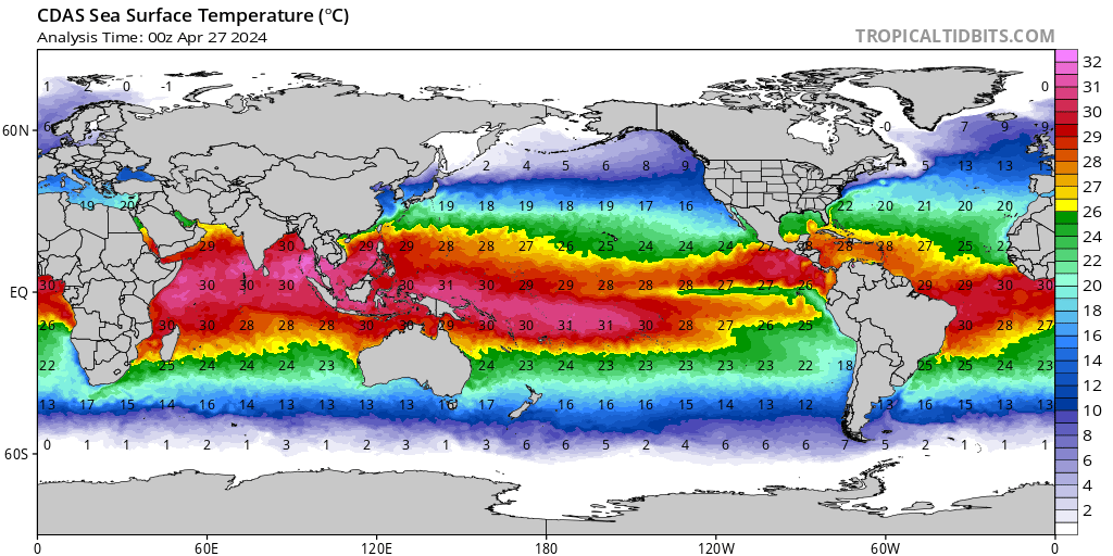
Thanks, Goldie, but it’s not clear to me just what you are calling the “ENSO regions” … could you please clarify that?
Thanks,
w.
The sea surface between 5N to 10N, and stretching from 150W to 120W. There was a sharp drop in temps across that zone. Here is what it looked like on Nov 6th. Then somewhere between the 6th and the 30th of November the temps in that area dropped. Looking back through my saved pics shows me that this is the coldest temps by far for this spot since at least 1 1 2016 when I started saving the daily pics.
This looks like the reason for the temp change. This is 500hPa. Note those cold winds which drop all the way down to 10N, carrying cold air south. The western boundary of that cold flow sits at 150W and extends to the east
Here is a look at November 30 2018 for comparison to the above current sst pic. This was about as cool as this section of the ocean had been over the last 5 years until the change in November of this year.
When do you think the upper limit of the temperature scale will need to be revised? All the climate models show the Nino34 region exceeding 32C this century and the Nino4 is warmer.
I think that we are in a gradual cooling trend that will steadily assert itself into the late 2030s. The speed of the temp change at this location was a surprise. It was like a switch was thrown and sea surface temps dropped up to 2C in this are (from 150W to 120W, and between 5N to 10N)., and have stayed several C cooler for around one month.
This current sudden shift in temps at this location is very interesting to me though. Look at how this cold air channel has formed a barrier between east/west air flows at 500 hPa. The air in the center is 3 to 6 C colder than air masses on either side, and this is connecting a mix of air from the two hemispheres. That is unusual compared to typical wind flows. It could possibly be a signal of a sea change of consequence in wind patterns…. https://earth.nullschool.net/#current/wind/isobaric/500hPa/overlay=temp/orthographic=-145.29,13.14,585/loc=-141.144,6.673
The highest thermal gradient is vertical, not equator to pole (much shallower thermal gradient).
What if a couple of degrees C of cumulative global cooling comes from cold air above continually sinking closer to the surface, and not from any increase whatsoever in the volume or regularity of equatorward directed polar air?
Everyone presumes the opposite to explain a cooling process, but there’s no need to presume that when by far the steepest T gradient is vertical. But far the simplest path to lower T difference is just overhead.
But we see that as a convective process, rather than convective, plus sinking air.
What if, for whatever reason, sinking air became much more popular than the past 40 years, instead of staying more than 15 km up?
(someone will be along shortly to say that is impossibles and every shade of heretical anti-meme crazy-talk)
Cod air only sinks if it is too cold for the height it is at.
Careful with the “only” word, that’s the general presumption, but not the practical observation.
When atmospheric waves enter the lower stratosphere it can be seen that they continue on their trajectory, but eventually the resulting chilled more humid air (-80C now) that was formerly tropospheric air, falls back into the troposphere, from the stratosphere, plus pulls stratospheric air down with it, and both mix in and warm from there, as they fall through the 30,000 ft level.
Note that I said, “for whatever reason”, not because it’s colder.
I’ll rephrase;
“What if, for an unknown reason, sinking air became much more popular than the past 40 years, instead of staying more than 15 km up?”
Several years ago Patrick Michaels wrote that the difference in temperature between the equator and poles is due to the difference in heat capacity of warm moist air and cold dry air. I global warming occurs there would be a smaller temperature difference which would mean fewer strong storms and winds.
Ed Z ==> Excellent, thank you.
The Poles are cold and the tropics are warm that is because the poles receive less sunlight then the tropics and any advection between them does not counteract this.