Nyquist, sampling, anomalies and all that

Guest post by Nick Stokes,

Every now and then, in climate blogging, one hears a refrain that the traditional min/max daily temperature can’t be used because it “violates Nyquist”. In particular, an engineer, William Ward, writes occasionally of this at WUWT; the latest is here, with an earlier version here. But there is more to it.

Naturally, the more samples you can get, the better. But there is a finite cost to sampling limitation; not a sudden failure because of “violation”. And when the data is being used to compile monthly averages, the notion promoted by William Ward that many samples per hour are needed, that cost is actually very small. Willis Eschenbach, in comments to that Nyquist post, showed that for several USCRN stations, there was little difference to even a daily average whether samples were every hour or every five minutes.

The underlying criticism is of the prevailing method of assessing temperature at locations by a combined average of Tmax and Tmin = (Tmax+Tmin)/2. I’ll call that the min/max method. That of course involves just two samples a day, but it actually isn’t a frequency sampling of the kind envisaged by Nyquist. The sampling isn’t periodic; in fact we don’t know exactly what times the readings correspond to. But more importantly, the samples are determined by value, which gives them a different kind of validity. Climate scientists didn’t invent the idea of summarising the day by the temperature range; it has been done for centuries, aided by the min/max thermometer. It has been the staple of newspaper and television reporting.

So in a way, fussing about regular sample rates of a few per day is theoretical only. The way it was done for centuries of records is not periodic sampling, and for modern technology, much greater sample rates are easily achieved. But there is some interesting theory.

In this post, I’d like to first talk about the notion of aliasing that underlies the Nyquist theory, and show how it could affect a monthly average. This is mainly an interaction of sub-daily periodicity with the diurnal cycle. Then I’ll follow Willis in seeing what the practical effect of limited sampling is for the Redding CA USCRN station. There isn’t much until you get down to just a few samples per day. But then I’d like to follow an idea for improvement, based on a study of that diurnal cycle. It involves the general idea of using anomalies (from the diurnal cycle) and is a good and verifiable demonstration of their utility. It also demonstrates that the “violation of Nyquist” is not irreparable.

Here is a linked table of contents:

  • Aliasing and Nyquist
  • USCRN Redding and monthly averaging
  • Using anomalies to gain accuracy
  • Conclusion

Aliasing and Nyquist

Various stroboscopic effects are familiar – this wiki article gives examples. The math comes from this. If you have a sinusoid frequency f Hz (sin(2π)) samples at s Hz, the samples are sin(2πfn/s), n=0,1,2… But this is indistinguishable from sin(2π(fn/s+m*n)) for any integerm (positive or negative), because you can add a multiple of 2π to the argument of sin without changing its value.

But sin(2π(fn/s+m*n)) = sin(2π(f+m*s)n/s) that is, the samples representing the sine also representing a sine to which any multiple of the sampling frequency s has been added, and you can’t distinguish between them. These are the aliases. But if s is small, the aliases all have higher frequency, so you can pick out the lowest frequency as the one you want.

This, though, fails if f>s/2, because then subtracting s from f gives a lower frequency, so you can’t use frequency to pick out the one you want. This is where the term aliasing is more commonly used, and s=2*f is referred to as the Nyquist limit.

I’d like to illuminate this math with a more intuitive example. Suppose you observe a running track, circle circumference 400 m, from a height, through a series of snapshots (samples) 10 sec apart. There is a runner who appears as a dot. He appears to advance 80 m in each frame. So you might assume that he is running at a steady 8 m/s.

But he could also be covering 480m, running a lap+80 between shots. Or 880m, or even covering 320 m the other way. Of course, you’d favour the initial interpretation, as the alternatives would be faster than anyone can run.

But what if you sample every 20 s. Then you’d see him cover 160 m. Or 240 m the other way, which is not quite so implausible. Or sample every 30 s. Then he would seem to progress 240m, but if running the other way, would only cover 160m. If you favour the slower speed, that is the interpretation you’d make. That is the aliasing problem.

The critical case is sampling every 25s. Then every frame seems to take him 200m, or halfway around. It’s 8 m/s, but could be either way. That is the Nyquist frequency (0.04 Hz), relative to the frequency 0.02Hz which goes with as speed of 8 m/s. Sampling at double the frequency.

But there is one other critical frequency – that 0.2 Hz, or sampling every 50s. Then the runner would appear not to move. The same is true for multiples of 50s.

Here is a diagram in which I show some paths consistent with the sampled data, over just one sample interval. The basic 8 m/s is shown in black, the next highest forward speed in green, and the slowest path the other way in red. Starting point is at the triangles, ending at the dots. I have spread the paths for clarity; there is really only one start and end point.

All this speculation about aliasing only matters when you want to make some quantitative statement that depends on what he was doing between samples. You might, for example, want to calculate his long term average location. Now all those sampling regimes will give you the correct answer, track centre, except the last where sampling was at lap frequency.

Now coming back to our temperature problem, the reference to exact periodic processes (sinusoids or lapping) relates to a Fourier decomposition of the temperature series. And the quantitative step is the inferring of a monthly average, which can be regarded as long term relative to the dominant Fourier modes, which are harmonics of diurnal. So that is how aliasing contributes error. It comes when one of those harmonics matches the sample rate.

USCRN Redding and monthly averaging

Willis linked to this NOAA site (still working) as a source of USCRN 5 minute AWS temperature data. Following him, I downloaded data for Redding, California. I took just the years 2010 to present, since the files are large (13Mb per station per year) and I thought the earlier years might have more missing data. Those years were mostly gap-free, except for the last half of 2018, which I generally discarded.

Here is a table for the months of May. The rows are for sampling frequencies of 288, 24, 12, 4, 2, and 1 per day. The first row shows the actual mean temperature averaged 288 times per day over the month. The other rows show the discrepancy for the lower rate of sampling, for each year.

Per hour  2010  2011  2012  2013  2014  2015  2016  2017  2018
1/12 13.611 14.143 18.099 18.59 19.195 18.076 17.734 19.18 18.676
 1 -0.012  0.007 -0.02 -0.002 -0.021 -0.014 -0.007  0.002  0.005
 2 -0.004  0.013 -0.05 -0.024 -0.032 -0.013 -0.037  0.011 -0.035
 6 -0.111 -0.03 -0.195 -0.225 -0.161 -0.279 -0.141 -0.183 -0.146
 12  0.762  0.794  0.749  0.772  0.842  0.758  0.811  1.022  0.983
 24 -2.637 -2.704 -4.39 -3.652 -4.588 -4.376 -3.982 -4.296 -3.718

As Willis noted, the discrepancy for sampling every hour is small, suggesting that very high sample rates aren’t needed, even though they are said to “violate Nyquist”. But they get up towards a degree for sampling twice a day, and once a day is quite bad. I’ll show a plot:

The interesting thing to note is that the discrepancies are reasonably constant, year to year. This is true for all months. In the next section I’ll show how to calculate that constant, which comes from the common diurnal pattern.

Using anomalies to gain accuracy

I talk a lot about anomalies in averaging temperature globally. But there is a general principle that it uses. If you have a variable T that you are trying to average, or integrate, you can split it:
T = E + A
where E is some kind of expected value, and A is the difference (or residual, or anomaly). Now if you do the same linear operation on E and A, there is nothing gained. But it may be possible to do something more accurate on E. And A should be smaller, already reducing the error, but more importantly, it should be more homogeneous. So if the operation involves sampling, as averaging does, then getting the sample right is far less critical.

With global temperature average, E is the set of averages over a base period, and the treatment is to simply omit it, and use the anomaly average instead. For this monthly average task, however, E can actually be averaged. The right choice is some estimate of the diurnal cycle. What helps is that it is just one day of numbers (for each month), rather than a month. So it isn’t too bad to get 288 values for that day – ie use high resolution, while using lower resolution for the anomalies A, which are new data for each day.

But it isn’t that important to get E extremely accurate. The idea of subtracting E from T is to remove the daily cycle component that reacts most strongly with the sampling frequency. If you remove only most of it, that is still a big gain. My preference here is to use the first few harmonics of the Fourier series approximation of the daily cycle, worked out at hourly frequency. The range 0-4 day-1 can do it.

The point is that we know exactly what the averages of the harmonics should be. They are zero, except for the constant. And we also know what the sampled value should be. Again, it is zero, except where the frequency is a multiple of the sampling frequency, when it is just the initial value. This is just the Fourier series coefficient of the cos term.

Here is are the corresponding discrepancies of the May averages for different sampling rates, to compare with the table above. The numbers for 2 hour sampling have not changed. The reason is that the error there would have been in the 8th harmonic, and I only resolved the diurnal frequency up to 4.

Per hour  2010  2011  2012  2013  2014  2015  2016  2017  2018
 1/12 -0.012  0.007 -0.02 -0.002 -0.021 -0.014 -0.007  0.002  0.005
 2 -0.004  0.013 -0.05 -0.024 -0.032 -0.013 -0.037  0.011 -0.035
 6  0.014  0.095 -0.07 -0.1 -0.036 -0.154 -0.016 -0.058 -0.021
 12 -0.062 -0.029 -0.075 -0.051  0.019 -0.066 -0.012  0.199  0.16
 24  1.088  1.021 -0.665  0.073 -0.864 -0.651 -0.258 -0.571  0.007

And here is the comparison graph. It shows the uncorrected discrepancies with triangles, and the diurnally corrected with circles. I haven’t shown the one sample/day, because the scale required makes the other numbers hard to see. But you can see from the table that with only one sample/day, it is still accurate within a degree or so with diurnal correction. I have only shown May results, but other months are similar.

Conclusion

Sparse sampling (eg 2/day) does create aliasing to zero frequency, which does affect accuracy of monthly averaging. You could attribute this to Nyquist, although some would see it as just a poorly resolved integral. But the situation can be repaired without resort to high frequency sampling. The reason is that most of the error arises from trying to sample the repeated diurnal pattern. In this analysis I estimated that just from Fourier series of hourly readings from a set of base years. If you subtract a few harmonics of the diurnal, you get much improved accuracy for sparse sampling of each extra year, at the cost of just hourly sampling of a reference set.

Note that this is true for sampling at prescribed times. Min/max sampling is something else.


0 0 votes
Article Rating
249 Comments
Oldest
Newest Most Voted
Inline Feedbacks
View all comments
Latitude
January 25, 2019 6:12 am

Thanks Nick

Reply to  Latitude
January 27, 2019 1:18 pm

Can someone ask Mr. Strokes
how there could be more sampling
( or any sampling!)
of those infilled numbers
— those pesky wild guesses
made by government bureaucrats
with science degrees,
required to compile a global average
SURFACE temperature?

And isn’t it puzzling that the surface
average is warming faster than the
weather satellite average … yet
weather satellite data, with far less
infilling, can be verified with weather
balloon data … but no one can verify
the surface data, because there’s no way
to verify wild guess infilling!

Only a fool would perform
detailed statistical analyses
on the questionable quality
surface temperature numbers,
(especially data before World War II),
and completely ignore the
UAH satellite data (simply because
satellite data shows less global warming,
and never mind that they are
consistent with weather balloon
radiosondes).

The greenhouse effect takes place
in the troposphere.

The satellites are in the troposphere.

How could the greenhouse effect
warm Earth’s surface faster than
it is warming the troposphere?

It can’t.

Three methodologies can be used
to make temperature measurements.

The outlier data are the surface
temperature data.

So why are they are the only data used?

This sounds like biased “science” to me !

My climate science blog
(sorry — no wild guess predictions
of the future climate —
that’s not real science!):
http://www.elOnionBloggle.Blogspot.com

Greg
January 25, 2019 6:30 am

Nick , you may want to review your markup. Your sin formulae in the Nyquist section are coming out with a umlaut-capital I and a large euro symbol. I’m guessing you want a lower case omega or something. It makes it very hard to read.

Reply to  Greg
January 25, 2019 7:31 am

Thanks, Greg. The mystery character is just pi. The HTML needs a line
<meta charset=”UTF-8″>
at the top, which I hope a moderator could insert, so that it can read extended Unicode characters. Oddly enough, the comments environment does this automatically, so I didn’t realise it was needed in posts. Here is the same html as it appears in a comment:
If you have a sinusoid frequency f Hz (sin(2πft)) sampled at s Hz, then the samples are sin(2πfn/s), n=0,1,2…
But this is indistinguishable from sin(2π(fn/s+m*n)) for any integer (positive or negative), because you can add a multiple of 2π to the argument of sin without changing its value.

But sin(2π(fn/s+m*n)) = sin(2π(f+m*s)n/s)

Reply to  Nick Stokes
January 25, 2019 9:20 am

Added that, but it doesn’t resolve the problem. I’m going to have to apply my brute force method to make π

Reply to  Anthony Watts
January 25, 2019 9:27 am

Fixed, please check to see if I missed anything.

Reply to  Anthony Watts
January 25, 2019 9:43 am

Thanks, Anthony. Everything seems fixed.

Reply to  Anthony Watts
January 25, 2019 9:51 am

Great, in the future, you can use alt-codes like alt-227 to make π

Jeff Alberts
Reply to  Anthony Watts
January 25, 2019 10:02 am

“Great, in the future, you can use alt-codes like alt-227 to make π”

I tried that, and all it did was make that weird symbol on my screen. I wanted some PIE!! 🙂

Hocus Locus
Reply to  Anthony Watts
January 28, 2019 1:46 am

Watts, Anthony. Cooking Up A Little `π’: Brute Force Recipes. WUWT WordPress, 2019. ISBN 314159265358-2

John Endicott
January 25, 2019 6:39 am

While I don’t have a problem with min/max per se, where I can see an potential issue is that the fewer samples you have the less likely your min is near the actual min and the max is near the actual max.

Compounding that is depending on when you take your samples you could be biasing the results without realizing it. For example if you only take 2 samples a day and one sample happens to be minutes away from the real max but the other sample happens to be hours away from the real min, you’ll have a bias towards warmer temps whereas in the reverse case it would bias you towards colder temps and in both cases a bias towards shorter spread of temps (IE real min is 10 real max is 60 for a spread of 50 verse sample min of 30 sample max of 50 for a spread of 20).

Obviously, the more samples you have the better accuracy of your min/max (versus the real min/max) reducing the potential for unintended bias and shortened spread. (instead of having samples that are minutes versus hours away from the min/max you can reduce that to seconds versus minutes for example).

As with all things, it’s a balancing act: in this case between having a high enough frequency to be reasonably accurate without the need for “repair” (which requires assumptions that might not, themselves, be entirely accurate) and the availability of resources to provide that frequency.

With modern tech, high frequency of sampling shouldn’t be all that difficult or expensive to achieve going forward (with less “human-error” in the mix, as computer-controlled sensors can do nearly all the grunt work for you). Obviously past samplings did not have such abilities.

Greg
Reply to  John Endicott
January 25, 2019 6:50 am

“Obviously past samplings did not have such abilities.” Hey that’s easy, you just need to “homogenise” the data and that will reduce the uncertainty by a factor of 10 , at least 😉

boffin77
Reply to  John Endicott
January 25, 2019 7:04 am

The old min/max thermometers were mechanical and sampled (effectively) infinitely often, saving only two of the samples – the min and the max. Infinite sampling frequency beats Nyquist every time.

MarkW
Reply to  boffin77
January 25, 2019 7:19 am

While the thermometer may be sampling an infinite number of times, as you say, only two of those numbers were saved. The min and the max.
What happens prior to all but the min and the max being saved isn’t relevant. Only two data points are passed on, and two data points does not satisfy Nyquist.

icisil
Reply to  boffin77
January 25, 2019 7:51 am

I call BS. No one sampled “infinitely often”.

John Endicott
Reply to  icisil
January 25, 2019 8:07 am

Indeed, while the thermometers may have been effective sampling “infinitely often” those samples where being recorded by human-hand only a small number of times a day (and of those, often only the min and max where then saved).

Loren Wilson
Reply to  icisil
January 25, 2019 9:37 am

Because you are working with a column of liquid metal, the rate of expansion is about the rate that the molecules of mercury are vibrating. This is in the nanosecond or microsecond range. I’ll allow his rounding off of millions to billions of states per second to infinite.

richard verney
Reply to  Loren Wilson
January 25, 2019 7:52 pm

The thermal lag (thermal inertia/response time) of an old LIG thermometer is such that the recomendation is to allow about 3 to 5 mins for the temperature reading to stabilise.

A LIG thermometer may be sampling on an infinite basis, but its response to change is not instantaneous and therefore it fails to record very short lived episodes.

Consider temperatures taken at airports where the station is situated near the runway/tarmac areas of the airport and the passing of a jet plane on a runaway which blasts warm air (possibly just that coming off the runway itself, not the exhaust of from the engine), an old LIG thermometer will not pick this up, whereas the modern electric thermal couple type thermometer will since the latter has a response time of less than a second.

There is a real issue of splicing together temperature measurements taken by LIG thermometers with those taken by modern electronic instruments.

Menicholas
Reply to  Loren Wilson
January 26, 2019 5:15 pm

You think a tube of glass filled with liquid metal responds in a microsecond to a change in temperature of the air it is immersed in?
A nanosecond?
This must be sarcasm.

JEHill
Reply to  Menicholas
January 26, 2019 5:40 pm

I may be wrong but I think that’s why he was given to infinity….

When you look at thermometer just like a speedometer it is an instantaneous moment in time. It is a scalar only the next measurement next gives any indication of direction or trend. But we know nothing of the system between one measurement to the next, any one of those billions of trillions states could have come into reality. The atmosphere is not a static system. Nor is it a colum of air moving only in the z-axis. Mixing, thermal density differentials, etc. all come into play.

Menicholas
Reply to  Loren Wilson
January 26, 2019 5:16 pm

I think we can be pretty sure you are not a nurse or anyone who has ever been in an actual laboratory.

Hlaford
Reply to  icisil
January 25, 2019 2:02 pm

Actually… there is a difference between FIR and IIR filters. The whole Nyquist hullabaloo here deals with FIR constraints. The whole nature works in terms of IIR filtering, and so do the temperatures. In a previous installment Vukcevic made a valuable note – put a thermometer in a big bucket of water (an IIR filter of a big time constant) and run a single temperature measurement per day. Bolometric measurements of power and energy measurements are gold standard in all other walks of technology – why climate is an exception?

Clyde Spencer
Reply to  boffin77
January 25, 2019 10:38 am

boffin77
But it is possible that the magnetic pins might move, introducing an unknown amount of error. No mechanical system is perfect.

boffin77
Reply to  Clyde Spencer
January 26, 2019 10:27 pm

Generally “sampling rate” means how often the “system” is observed. If there is thermal inertia, that is part of the system, not the sampler. If there are errors due to magnetic pins moving, that introduces an error, but does not change the sampling rate. If the LIG thermometer has e.g. stiction and is thus not instantaneous, then that introduces an error (or if intentional then that introduces a low-pass filter upstream of the sampler) but does not change the sampling rate.
To assess the sampling rate, in a mechanical system (which I suggest is not a helpful exercise as illustrated by many comments) then you might ask a question such as: if the liquid magically rises by one degree for a very short time t, and then drops again, what is the longest value of t that might be completely missed by the detector?

Robert Stewart
Reply to  boffin77
January 25, 2019 10:47 am

All physical thermometers have some amount of thermal inertia, which means that their “max” is something other than the true max unless the thermometer is soaked at that max for a very long time. Which, of course, they are not.

It is also the case that the Nyquist folding theorem applies to stationary systems, and nothing could be farther from the truth, particularly on seasonal-, let alone climatological-, time scales. As anyone who understands “climate” knows. Particularly all of us who are accused of being “climate deniers”. These min/max historical thermometer readings, and the old bucket sea surface temperatures, may be a source of present-day employment, and they are better than nothing, but not much. The paintings of ice fairs on the Thames River probably have much more significance in understanding climate change, than 90% of the min/max surface temperatures.

D Cage
Reply to  boffin77
January 25, 2019 11:02 pm

Except being mechanical it was only accurate to around a quarter of a degree from a test I did to see the difference between a quite expensive mechanical one I had and its new fancy electronic equivalent.
It sometime stuck low and at others seemed to overshoot. Quite how the mechanism of moving the pin worked in practice I am not really sure given the meniscus on top of the mercury and friction holding the pin in place.
Also two different electronic thermometers had different response times one similar to the mechanical one and one much faster which showed higher peaks but strangely not so different low ones.

Gary Wescom
Reply to  John Endicott
January 25, 2019 8:19 am

I am of the opinion that concerns about Nyquist sampling rate are irrelevant to analysis of max/min daily temperatures. The question should be how does max/min daily sampling compare with a true average. Data from the USCRN allow us to examine that question. I did some quick studying along those lines:

http://climate.n0gw.net/TOBS.pdf

A C Osborn
Reply to  Gary Wescom
January 25, 2019 1:33 pm

Gary, the major question for me is that everyone for TOBS says that you can get a false reading by getting a low or high from the previous day etc, which you have shown.
The big question for me is “How Often Did It Actually Happen”?
Because they adjust all the readings, which means that they could be adding a much bigger bias when the frequency of a actual TOBS errors is low.
Say it happens once per month, that means that they correct one value and make incorrect 27-30 others.
So do we have any idea how often it actually happened?

Gary Wescom
Reply to  A C Osborn
January 25, 2019 8:06 pm

A C
Nope, I don’t know and neither does anyone else. The mitigating factor here is the correction is applied as a small bias on monthly data, though that amount is based upon some thin guesswork.

Menicholas
Reply to  A C Osborn
January 27, 2019 4:41 pm

Tony Heller did an analysis of this very question, and what he found was that when comparing two sets of records, it can be shown that TOB is completely bogus.
So many issues with it that are clearly intended to artificially create a warming trend that matches the CO2 concentration graph.
Like how the TOB adjustment somehow went from .3 F to .3 C, sometime between USHCN V2 and V3.
Here is a link to a whole bunch of postings he has done on the subject.
The top one has a graph where he simply compared the stations which measured in the afternoon to the ones which measured in the morning.
The only real difference in the two sets is that stations recording in the morning tend to me more southerly, and hence hotter, because in hot places people like to go out in the morning more.
https://realclimatescience.com/2018/07/the-completely-fake-time-of-observation-bias/

https://realclimatescience.com/?s=Time+of+observation

michel
January 25, 2019 6:39 am

Many thanks to Nick for taking what must have been quite a bit of trouble to lay all this out. And many thanks to WUWT for featuring a contribution from one of the community’s leading contrarians!

Its this spirit of inclusion, that you won’t find on Ars or Real Climate, or the Guardian, and of course never on Skeptical Science, that keeps many of us coming back here. We positively like being challenged and made to think, and we greatly value WUWT for being a place which will feature alternative points of view.

Good on you!

Tonyb
Editor
Reply to  michel
January 25, 2019 8:52 am

Let’s endorse that comment. Whether we agree with him or not, nick is one of the only people offering counter views here and it makes us stop and think. He is also patient and polite.

Tonyb

Greg
January 25, 2019 6:48 am

Interesting article Nick. However, in order to remove the daily cycle you do need hires data. There is not guarantee that past diurnal cycle was the same as present. I’m not clear on what use you are suggesting could be made of this.

What kind of aliasing issues do you think could result from taking “monthly” ( 30/31 day ) averages in the presence of 27 or 29 day lunar induced variations?

Reply to  Greg
January 25, 2019 8:07 am

Greg,
Most of the error in monthly average results from the interaction of the sampling frequency with harmonics of the diurnal frequency. So if you subtract even a rough version of the latter, you get rid of much of the error. Even one year gives you 30 days to estimate the diurnal cycle for a particular month. I just calculated the first few Fourier coefficients of this (I used 2010-2018) based on hourly sampling. Then when you subtract that trig approx, you can use coarse (eg 2/day) sampling with not much aliasing from diurnal, and the trig approx itself can be integrated exactly to complete the sum.

IanH
Reply to  Nick Stokes
January 25, 2019 12:13 pm

but weather can vary so much over a few days, here we’ve had freezing conditions for days, but a front has come through and we have balmy temps today.

Javert Chip
January 25, 2019 6:50 am

This post by Nick (whom I know is a controversial poster) is a perfect example of why I read WUWT. As an old CFO, I understand sampling & statistical tricks, but I respect Nick’s reasonably objective approach to the discussion..

It’ll be interesting to read other, more qualified WUWT responses to Nick, but I appreciate that this discussion has been started at a technical level.

Matthew Drobnick
Reply to  Javert Chip
January 25, 2019 1:31 pm

Javert, I agree. In fact, I now look forward to reading his comments and his infrequent posts. It helps me remain balanced, but at first I resisted it. Can’t be just another echo chamber person.

I’m also enjoying reading Mr. Mosher, now that he’s not just tossing in fly by snark but lengthy input.

Given our current climate of censorship, this is refreshing. Truly, wuwt is the highest quality content site on the matter

coaldust
January 25, 2019 6:52 am

I didn’t read the whole post, but the idea of Nyquist being important in temperature sampling is wrong. Nyquist tells us how often periodic samples are needed to reconstruct the waveform. Who cares about reconstructing the whole temperature waveform?

Still I think min & max and time of min & max plus some periodic sampling makes sense. That way more reliable statistics such as mean and standard deviation can be developed. (Tmin + Tmax)/2 is not an accurate mean.

Also humidity is important to measure as well as temperature.

MarkW
Reply to  coaldust
January 25, 2019 7:26 am

If you want to accurately calculate the daily average temperature, you need to be able to accurately reconstruct the waveform.
If you want to accurately calculate a monthly average temperature, you need accurate daily average temperatures.

matthewdrobnick
Reply to  MarkW
January 25, 2019 8:16 am

honest questions:

Have we ever had truly accurate daily average temperatures?
If so, when and what time period?
If so, are there separate methods of collecting this data that are different but also considered accurate and how are they reconciled against each other?

Additionally, how can it be stated we have resolution down to .0x C? that seems highly improbable going back any length of time

MarkW
Reply to  matthewdrobnick
January 25, 2019 9:01 am

The newer sensors log hourly readings, which is good enough for government work.
I believe they started rolling out the newer style sensors sometime in the 1970’s.

The claim is that if you average together a bunch of readings that are accurate to 1 degree C, then you can improve the accuracy. Bogus, but they still make that claim.

Jim Gorman
Reply to  MarkW
January 25, 2019 12:36 pm

You are right, this claim is bogus. I am working on an essay that I’ll finish one of these days.

To calculate an uncertainty of the mean (increased accuracy of a reading) you must measure the SAME thing with the same instrument multiple times. The assumptions are that the errors will be normally distributed and independent. The sharper the peak of the frequency distribution the more likely you are to get the correct answer.

However, daily temperature reading are not the same thing! Why not? Because the reading tomorrow can’t be used to increase the accuracy of today’s readings. That would be akin to measuring an apple and a lime and recording the values to the nearest inch, then averaging the measurements and saying I just reduced the error of each by doing the average of the two. It makes no sense. You would be saying I reduced the error on the apple from 3 inches +- 0.5 inch to 3 inches +- 0.25 inches.

The frequency distribution of measurement errors is not a normal distribution when you only have one measurement. It is a straight line at “1” across the entire error range of a single measurement. In other words if the recorded temperature is 50 +- 0.5 degrees, the actual temperature can be anything between 49.5 and 50.5 with equal probability and no way to reduce the error.

Can you reduce temperature measurement error by averaging? NO! You are not measuring the same thing. It is akin to averaging the apple and lime. Using uncertainty of the mean calculations to determine a more accurate measure simply doesn’t apply with these kind of measurements.

So what is the upshot. The uncertainty of each measure must carry thru the averaging process. It means that each daily average has an error of +- 0.5, each monthly average has an error of +- 0.5, and so on. What does it do to determining a baseline? It means the baseline has an error of +- 0.5 What does it do to anomalies? It means anomalies have a built in error of +- 0.5 degrees. What does it do to trends? The trends have an error of +- 0.5 degrees.

What’s worse? Taking data and trends that have an accuracy of +- 0.5 and splicing on trends that have an accuracy of +- 0.1 degrees and trying to say the whole mess has an accuracy of +- 0.1 degrees. That’s Mann’s trick!

When I see projections that declare accuracy to +-0.02 degrees, I laugh. You simply can not do this with the data measurements as they are. These folks have no idea how to treat measurement error and even worse how to program models to take them into account.

Nyquist errors are great to discuss but they are probably subsumed in the measurement errors from the past.

Matthew Drobnick
Reply to  MarkW
January 25, 2019 1:20 pm

Thank you Mark and Jim for the response. This is the major issue I’ve seen, among many, that initially zipped past me. Upon further inspection this seems so glaring I don’t know how I missed it.
To be fair I used to only read or watch MSM. Imagine that

Menicholas
Reply to  MarkW
January 26, 2019 5:40 pm

Stick around, and hear from all of the people that will argue over and over again for days and weeks on end that measuring temps in different places and on different days, can all be used to reduce the error bars in global average temps to an arbitrarily small number, even if the original measurement resolutions are orders of magnitude higher.
They refuse to accept that it is not a whole bunch of measurements of the same thing, nor to acknowledge that the techniques used are only valid under circumstances that do not apply, normal distribution, not auto correlated, etc.
These same people also commonly confuse and conflate terms such as precision and accuracy.
Just wait, they will be here.

JEHill
Reply to  Menicholas
January 26, 2019 6:10 pm

And to follow up…

Even if they were mathematically valid, followed high metrology standards, on well maintained and validated instruments average global temperature has very little meaning on a mechanical system as large as the Earth.

Sure that Earth has warm a bit since 1850 but nothing I read suggests that the climate anywhere has changed. The Sahara is the Sahara, tropics are still here, the temperate zones are still temperate and have seasons…

James Schrumpf
Reply to  MarkW
January 26, 2019 11:46 pm

I’ve done some studying lately about the Law of Large Numbers and how it’s used to reduce the error in the mean. It’s also described as a probability tool, and a way to determine the increase in the probability that a single measurement will be close to the expected value.

In both those cases, the emphasis is on “the expected value,” whether it’s the probability of flipping a coin and getting heads or measuring the length of a board.

However, in climate science, there IS no “expected value.” Taking one max/min/avg temperature measurement per day and then averaging them and determining anomalies from them is like giving the person at each weather station a board to measure once day, and that board being up to one meter different from another. What’s the “expected value” that we’re approaching in this case? Sure, we can run the calculations, but there’s know way of knowing if there’s even a board out there equal to the length of the numbers we generate.

But I think there’s another, less obvious misuse of the Law of Large Numbers. To stick with the metaphor of the vastly different boards being measured, the LLN is only being applied piecemeal. Rather than taking all of the measurements from all of the boards that were measured, only the measurements from one board were used to create a local baseline for that station, and then its anomalies are created. After generating the local anomaly, the local anomalies from the rest of the world are then averaged and schussed and plotzed and whatever to make the global board anomaly — and then the LLN is applied to get that error in the mean as small as possible.

I’ll bet the statistics would be much different if a true global baseline was generated from the measurements from all of the world’s stations put together, and then the individual stations were compared with that. I’ll bet that standard deviation and error in the mean would look a lot different then.

JEHill
Reply to  James Schrumpf
January 27, 2019 12:16 am

Quote James Schrumpf:

“In both those cases, the emphasis is on “the expected value,”….

*****
In my mind this is one the logic fallacies in the AGW realm. The atmospheric temperature just “is” due to a whole bunch of inputs/outputs that are neither good or bad they just “are”.

We humans are not arbiters of that “is”.

While this discussion is may be useful for pushing statistics and math to a more rigorous discipline I am sure not it furthers climate theory. Especially until we have more rigorous instrument quality control. In addition to temperatures, I would like wind speed, humidity, barometric pressure, a way to measure the uplift of the air mass, perhaps some IR measurements looking up/down.

Gator
Reply to  JEHill
January 27, 2019 5:57 am

Don’t get me started… again… too late…

Temperature “anomalies” are derived from an incredibly insignificant blip of time on Earth, and using this incredibly small and meaningless set of numbers to understand an almost incomprehensible reality, is simply nonsense and self delusion.

a·nom·a·ly əˈnäməlē/ noun
1. -something that deviates from what is standard, normal, or expected.

1- There is no such thing as “normal” in climate or weather.

2- What exactly am I supposed to expect in the future, based upon the range of possibilities we see in the geologic record? Can the changes we see happening now be called “extreme” in any way?

3- No.

Anomalies are created by the definers of “normal”, and the deniers of climate history.

Jim Gorman
Reply to  MarkW
January 27, 2019 4:57 pm

James S. –> “I’ve done some studying lately about the Law of Large Numbers and how it’s used to reduce the error in the mean. It’s also described as a probability tool, and a way to determine the increase in the probability that a single measurement will be close to the expected value. ”

You missed the point. The law of large numbers and the uncertainty of the mean only deal with measurements of the same thing. If you pass around a board and a ruler to many people and ask them to measure it, you “may” be able to determine that the error of the mean is close to the true value. However, this requires that the errors are random and have a normal distribution.

You can’t measure one board and record it’s length to the nearest inch, then measure another board and say the errors offset so that you more closely know the true measurement of either board. You have no way to know if the first board was 40.6 and recorded as 41 or if it was 41.4 and recorded also as 41. And remember, it could be anywhere between those values. So each and every value you come up with will have the same probability with no way to cancel it out. The same applies to the second board.

When you average the two values, the average will never be better than the original measurement error, i.e. +/- 0.5 inches. That is because (41.4 + 41.4)/2 is just as likely as (40.6 + 40.6)/2 and is just as likely as (41.0 +41.0)/2.

Using the law of large numbers and the uncertainty of the mean calculations to reduce error requires:

1. measuring the same thing,
2. Multiple measurements of the same thing,
3. a normal distribution of errors.

Measuring temperatures at different times means you are not measuring the same thing, not doing multiple measurements of the same thing, and you have no errors to statistically use so you can’t have a normal distribution.

James Schrumpf
Reply to  MarkW
January 27, 2019 5:54 pm

Jim Gorman ->”You missed the point. The law of large numbers and the uncertainty of the mean only deal with measurements of the same thing. If you pass around a board and a ruler to many people and ask them to measure it, you “may” be able to determine that the error of the mean is close to the true value. However, this requires that the errors are random and have a normal distribution.

“You can’t measure one board and record it’s length to the nearest inch, then measure another board and say the errors offset”

I thought I was saying something like that when I wrote ” Taking one max/min/avg temperature measurement per day and then averaging them and determining anomalies from them is like giving the person at each weather station a board to measure once day, and that board being up to one meter different from another. What’s the “expected value” that we’re approaching in this case? Sure, we can run the calculations, but there’s know way of knowing if there’s even a board out there equal to the length of the numbers we generate.”

I’m pretty sure we’re in agreement on this one.

William Ward
Reply to  MarkW
January 27, 2019 8:24 pm

Jim,

You said: “Nyquist errors are great to discuss but they are probably subsumed in the measurement errors from the past.”

In my post, that Nick referenced, in one of my replies I stated my list of 12 things that are wrong with our temperature records. (I probably forgot one or two that could be added to the list). The general thrust of that post and the one Nick made here, is to focus on Nyquist exclusively. I believe all of the sources of error are cumulative. Maybe this would put us in agreement, Jim. I just wanted to make sure you know we are focusing on one thing here to study it. Maybe in the future and attempt will be made by someone to look at the record error comprehensively (all sources). In my experience, I have seen very little made of Nyquist violation as it relates to the instrumental record. So I wanted to detail that and hopefully add this to the ongoing discussion.

Climate Alarmists (and I’m not referring to anyone in particular – just generically) claim that science is completely on their side. Nyquist is one thing that refutes that – and one that cannot easily be dismissed because a comparison between methods can be made that shows the error in a mathematically conclusive and unambiguous way. All of the other problems with the record can be dismissed by Alarmists because there is no conclusive way to measure the effective error.

Reply to  MarkW
January 27, 2019 10:33 pm

“The law of large numbers and the uncertainty of the mean only deal with measurements of the same thing.”
“However, this requires that the errors are random and have a normal distribution.”

Often said here, but never with any support or justification quoted. And it just isn’t true. There is no requirement of “same thing”, nor of normal distribution. The law just reflects the arithmetic of cancelling ups and downs.

Jim Gorman
Reply to  MarkW
January 28, 2019 11:34 am

William Ward –> I didn’t mean to demean the value of determining the Nyquist requirements for calculating the necessary measurements. I think the value being placed on the past temperature data is ridiculous for many reasons of different errors. It is not fit for the purpose for which it is being used. I agree with your Nyquist analysis. I learned about Nyquist at the telephone company is the days when we were moving from analog carriers and switches into digital carriers and switches.

These errors along with measurement errors have never been addressed in a formal fashion in any paper I can find. I have all the BEST papers I can find and I only find statistical manipulations as if these are just plain old numbers being dealt with. No discussion at all about how the measurement errors affect the input data or how it affects the output data. I have yet to see a paper that discusses how broad temperature errors affect the outcomes of studies. Let alone how does the “global temperature” get divided down into a, for example, 100 acre plot where a certain type of bug population has changed. Too many studies simply say, “Oh global temperatures have risen by 1.5 degrees, so the average temperature in Timbuktu must be increased by 1.5 degrees also”. How scientific.

Jim Gorman
Reply to  MarkW
January 28, 2019 3:58 pm

NS –>

Remember, temperature measurements are not of the same thing. Each one is independent and non-repeatable once it has been recorded. That means N=1 when you are calculating error of the means.

Here are some references.

http://bulldog2.redlands.edu/fac/eric_hill/Phys233/Lab/LabRefCh6%20Uncertainty%20of%20Mean.pdf

Please note the following qualifiers:
1) “This means that if you take a set of N measurements of the same quantity and those measurements are subject to random effects, it is likely that the set will contain some values that are too high and some that are too low compared to the true value. If you think of each measurement value in the set as being the sum of the measurement’s true value and some random error, what we are saying is that the error of a given measurement is as likely to be positive as negative if it is truly random. ”
2) “There are three different kinds of measurements that are not repeatable. The first are intrinsically unrepeatable measurements of one-time events. For example, imagine that you are timing the duration of a foot-race with a single stopwatch. When the first runner crosses the finish line, you stop the watch and look at the value registered. There is no way to repeat this measurement of this particular race duration: the value that you see on your stopwatch is the only measurement that you have and could ever have of this quantity.”

https://en.wikipedia.org/wiki/Normal_distribution

Please note the following qualifier:
1) “Physical quantities that are expected to be the sum of many independent processes (such as measurement errors) often have distributions that are nearly normal.[3] Moreover, many results and methods (such as propagation of uncertainty and least squares parameter fitting) can be derived analytically in explicit form when the relevant variables are normally distributed. ”

https://users.physics.unc.edu/~deardorf/uncertainty/definitions.html

https://www.physics.umd.edu/courses/Phys276/Hill/Information/Notes/ErrorAnalysis.html

Please note the following qualifier:
1) “Random errors often have a Gaussian normal distribution (see Fig. 2). In such cases statistical methods may be used to analyze the data. The mean m of a number of measurements of the same quantity is the best estimate of that quantity, and the standard deviation s of the measurements shows the accuracy of the estimate. The standard error of the estimate m is s/sqrt(n), where n is the number of measurements. ”

https://encyclopedia2.thefreedictionary.com/Errors%2c+Theory+of

http://felix.physics.sunysb.edu/~allen/252/PHY_error_analysis.html

Reply to  MarkW
January 28, 2019 5:45 pm

Jim Gorman,
“Here are some references.”
None of them say that “The law of large numbers and the uncertainty of the mean only deal with measurements of the same thing.”. In fact, I didn’t see a statement of the LoLN at all. The first is a lecture from a course on measurement. It says how you can calculate the uncertainty for repeated measurements using LoLN. It doesn’t say anywhere that the LoLN is restricted to this.
Your next, Wiki link, says exactly the opposite, and affirms that the LLlON applies regardless of any notion of repeating the same measurement. It says:
“The normal distribution is useful because of the central limit theorem. In its most general form, under some conditions (which include finite variance), it states that averages of samples of observations of random variables independently drawn from independent distributions converge in distribution to the normal”
Nothe that they ate talking explicitly about the mean of non-normal variates (the mean tends to normal). And in the later Central Limit Theorem, there is a para starting:
“The central limit theorem states that under certain (fairly common) conditions, the sum of many random variables will have an approximately normal distribution. More specifically, …”
There is too much math to display here. But they say that if you have N iid (not normal) random variables variance σ, take the mean, and multiply by √N, the result Z has variance σ. So the mean has variance σ/√N. It converges to zero, which is the LoLN result. They give various ways the iid requirement can be relaxed.

The unc reference is also metrology. It has no LoLN, but simply says:
“standard error (standard deviation of the mean) – the sample standard deviation divided by the square root of the number of data points”
Same formula – no requirement of normality or “measuring the same thing”.

The UMD reference says that you can use these formulae for repeated, normal measurements, which is their case. It doesn’t say that usage is restricted to that.

The FreeDict, which is from the Soviet Encyclopdedia (!), again makes no general statement of LoLN.

Finally, the sunnysb ref, again no statement. But see the propagation of errors part. This says that “Even simple experiments usually call for the measurement of more than one quantity. The experimenter inserts these measured values into a formula to compute a desired result.”
And shows how the same formulae apply in combining such derived results.

So in summary – first, no requirement of normality, anywhere. Nor a general statement of LoLN. What has happened is that you have looked up stuff on repeated measurements, seen LoLN formulae used, and inferred that LoLN is restricted to such cases. It isn’t.

Jim Gorman
Reply to  MarkW
January 29, 2019 7:25 am

NS –> Rather than refuting each of your points, let me point out that I’m not trying to derail the central limit theorem or the law of large numbers. However, you are not seeing the forest for the trees.

Here is a story. A factory was producing rods that were to be a certain length. Last week they produced 1000 of them. The boss came to the production manager and said why did we get back 2/3 of the rods because some were too long and some too short. The manager said “I don’t know. I measured each one to the nearest inch, found the mean and the error of the mean. The error comes out to +/- 0.0002 inches.” The boss said, “Dummy, you just found out how accurate the mean was, not the error range of the production run.”

You are trying to prove the same thing. By averaging 1000 different independent temperature readings you can find a very accurate mean value. However, the real value of your average can vary from the average of the highest possible readings to the average of the lowest possible readings. In other words, the range of the error in each measurement.

Engineers deal with this all the time. I can take 10,000 resistors and measure them. I can average the values and get a very, very accurate mean value. Yet when I tell the designers what the tolerance is, can I use the mean +/- (uncertainty of the mean), or do I specify the average +/- (the actual tolerance) which could be +/- 20%?

I don’t know how else to explain it to you. Uncertainty of the mean and/or law of large numbers only has application to measurements of the same thing. And then they are only useful for finding an estimate of the true value of that one thing. When using single non-repeatable measurements the average is only useful when it is used with the error range of possible values.

William Ward
Reply to  MarkW
January 29, 2019 8:57 pm

Hi Jim,

Thanks for your follow-up comments. I didn’t take that you were demeaning the value of Nyquist, I was just adding some thoughts. I interpret that our views are very much in sync. Thanks for taking the time to clarify though. I do appreciate it. I whole heartedly agree with your follow-up comments. There is so much effort to crunch and analyze data that is bad and so little effort to question the validity of the data being crunched. Climate science has devolved to polishing the turd.

Editor
January 25, 2019 6:59 am

Back before max/min thermometers, it looks like people were more inclined to record the typical temperature of the day. For example, when I wrote my anniversary piece on the Year without a Summer, https://wattsupwiththat.com/2016/06/05/summer-of-1816-in-new-hampshire-a-tale-of-two-freezes/ , I was surprised at the temperature sampling used at various sites.

The one I focused on in Epping NH used “William Plumer’s temperature records were logged at 6:00 AM, 1:00 PM, and 9:00 PM each day. That sounds simple enough, and it turns out that several people in that era logged temperature data at those times or close to it.” One thing I adopted, and was common the, was to compute an average by counting the 9:00PM temperature twice. Clearly people were trying to avoid the extremes at dawn and after noon.

John Sims
January 25, 2019 6:59 am

Nick, You have attributed accuracy where there is none you anomaly scenario. You define E as an expected value (average) over a baseline. But is NOT an fixed number but a representative of a distribution (average and standard deviation, etc). That means that T is subject to the inherent error of both E and A and THAT is where I have issue with most climate scientists and the use of anomalies.

If you choose absolute zero for E then T=A and you eliminate the error around E. This shows the error of T = error A which should be the best you can get.

That said, I actually agree with your conclusions on station sampling data and frequency.

kent beuchert
January 25, 2019 6:59 am

My belief is that you cannot squeeze more information out of data than is actually there.
I don’t buy into data manipulation as a means of materializing non-existent information.

Greg
Reply to  kent beuchert
January 25, 2019 7:20 am

Nick was not suggesting materializing non-existent information. He was suggesting minimizing induced errors that degrade the available information.

All data processing is “data manipulation” , you are not saying anything.

icisil
Reply to  kent beuchert
January 25, 2019 7:41 am

But that’s climate science’s modus operandi.

Paramenter
Reply to  kent beuchert
January 27, 2019 2:41 pm

My belief is that you cannot squeeze more information out of data than is actually there.

Quite correct. Nick is using additional sources of information, not available in the original dataset, to reduce errors in this original dataset.

January 25, 2019 7:00 am

The actual problem with global annual average temperature as it relates to global warming is not the rate of sampling. I struggled with the rate problem because historically different records took measurements at different hours of the day. Few of them did a Min/Max and the hours of sampling reflected the individuals predliction or daily work schedule. I know from discussion with Hubert Lamb it was an issue with Manley’s Central England temperature.

It is reasonable to argue that the objective is detection of change over time and that can be detected regardless of the rate of sampling as long as it is consistent. Stokes tacitly acknowledges this with his selection of sample period because of misssing data in the earlier record.

No, the real problem with the calculation of a global average is the density of stations. It is inadequate in all but a couple of small areas and they are usually the most compromised by factors like the Urban Heat Island Effect or other site change.

John Tillman
Reply to  Tim Ball
January 25, 2019 8:17 am

So many things are wrong with average temperature reconstructions, both from statistical necessity and out of ideologically-motivated “adjustment”, that they are totally unfit for the purpose of guiding public policy.

matthewdrobnick
Reply to  John Tillman
January 25, 2019 8:33 am

as a person with non-STEM background, and after a few years of researching, I agree with your conclusion John. If the average citizen spent the time I have they would likely reach the same conclusion, because reaching a different conclusion necessarily omits so much collusion, inaccuracy, and fraud to be considered an erroneous conclusion.

What is scary is that when you start to peel back the layers of the official narrative, in almost every field, it becomes obvious just how much of the “narrative” is exactly that, a narrative.

I would argue that is where studying Poly Sci assists in these discussions, because I’m willing to recognize patterns about the politics and money, study history, read the words of people in positions of power and influence and see if they said has manifested, and tie them all in together from all sorts of arenas in life. Whereas, many of the STEM focused commentators on this site refuse to accept the conclusions of all that research and perspective because it makes them uncomfortable, for the exact same reasons I was uncomfortable after finally concluding CAGW was a scam. Additionally, many are hyperfocused on the math and subsequently suffer from tunnel vision. We need a balance of macro and micro perspectives.

It is a serious flaw of the human experience, and that is that not only can we lie to ourselves but we inherently don’t want to believe people are capable of such nefarious intent. More specifically, that we could also be fooled by others so easily. Much of what the good book teaches about good and evil is merely trying to drill into peoples heads how easy the path of deception is compared to a righteous path of honesty.

John Tillman
Reply to  matthewdrobnick
January 25, 2019 10:58 am

Matthew,

As a putative social “science”, polisci does at least use statistics. IMO even a single undergrad course in statistics suffices to call BS on the whole CACA house of cards (an ineptly mixed metaphor, I know).

The very few good land stations with long histories could be reconstructed. But on some continents, there might not be even one fit for purpose. It would take at least dozens to derive an even remotely representative land surface “record”. GISS’ Gavin Schmidt believes that only 50 stations would suffice. But that still leaves the 71% of Earth’s surface which is ocean.

The sea “surface” (actually below the surface, obviously) “record” is even more of a shambles than that for a bit above the ground.

IMO we can fairly say that Earth as a whole is a bit warmer now than 160 years ago, at the end of the Little Ice Age Cool Period, but pretending precision and accuracy to tenths of a degree would be laughable, if not such a sadly lethal scam. Moreover, most of whatever warming has occurred happened before WWII, when man-made CO2 was a negligible factor, at best.

It’s thus impossible to separate whatever human effect there might be from warming or cooling which would have occurred in the absence of our emisions. We can’t even know the sign of any human influence, since our particulate pollution as cooled the surface. Western Europe and America have cleaned up their air, but then along came China and India to fill it with soot and sulfur compounds anew.

Menicholas
Reply to  matthewdrobnick
January 27, 2019 3:36 am

Matt Drobnick,
“Much of what the good book teaches about good and evil is merely trying to drill into peoples heads how easy the path of deception is compared to a righteous path of honesty.”

It is interesting to note that there are realms in which such matters are dealt with in a serious way, every day of the week, and that is within courts of law.
Juries are instructed that if a witness is shown to have given deceptive testimony, in any particular detail, that witness can be assumed to be completely unreliable about anything and everything they have said. IOW, if you know a person is a liar, it is reasonable to ignore them completely, since they might be lying about everything or mixing truth and lies in ways which are unknowable.

And on this:
“It is a serious flaw of the human experience, and that is that not only can we lie to ourselves but we inherently don’t want to believe people are capable of such nefarious intent. More specifically, that we could also be fooled by others so easily. ”

I think it might well be the case that this is getting at a principle difference in the thought processes between people who are skeptical of such things as CAGW and the warmista narrative in general, and those who tend to have swallowed the whole yarn and cannot be convinced to question any of it, whether it be from MSM hype-meisters, prominent alarmists in the climate science orthodoxy, or any of the various breeds of shills and apologists for The Narrative.

The cognitive dissonance of even intelligent people on such matters, especially if they are politicize to such an enormous degree, can be utterly blinding and deafening to those so affected. They can be shown an veritable infinitude of instances of proven and blatant fraud in such areas as academia, medicine, law, justice, and scientific research, and somehow refuse to accept that there is fraud involved in anything important. Or even that sometimes people who are sure they are correct, are simply wrong. Or that people who have spent a career going out on a limb with predictions of some thing, might be inclined to do anything they can to prevent being proven wrong.
The actual situation we are in is much worse than a few random people maybe getting a few things wrong, or overlooking any information which is contrary to what they are selling.
We know there are people who never cared what was true or not, because it was The Narrative that was important.
We know that huge numbers of people have painted themselves into a corner with the certainty they have expressed about something which is dubious at best.

Given the stakes in all of this, the money, prestige, power, fame, influence, etc…and given the consequences of being proven wrong, of not simply losing some money, or prestigious and lucrative careers, or power and influence, political or otherwise, but of being disgraced and discredited, and in some cases possibly culpable of indictable criminal and civil offenses.

Following a train of thought to it’s logical conclusion takes one rather far afield from the discussion at hand, but it is impossible to understand some things without having a far larger perspective.

John Tillman
Reply to  Menicholas
January 27, 2019 2:31 pm

Sadly, none of today’s shameless charlatans spewing CACA is liable ever to be held legally accountable to the millions of deaths and trillions in lost treasure which their anti-human scam has cost.

Jim Gorman
Reply to  Tim Ball
January 25, 2019 1:19 pm

You are not mentioning the measurement errors when temperatures are recorded to the nearest degree. A lot of the early temperature measurements had errors of +- 0.5 degrees and there is really no way to remove this error range since each measurement is a stand alone measurement. You may determine a trend, but only to the same accuracy. Most projections don’t even come close to exceeding this error range so are nothing but noise.

William Ward
Reply to  Tim Ball
January 27, 2019 8:37 pm

Hi Tim,

This post from Nick and my post that initiated it, focused on temporal aliasing. Spatial aliasing is also a critical problem – but not explored here.

You said: “The actual problem with global annual average temperature as it relates to global warming is not the rate of sampling. …”

My reply: Did you read my post (particularly the FULL paper)? That shows with actual examples from USCRN how sample rate matters. Analysis done by Willis added to that, showing significant improvements from 2-samples/day to 24-samples/day when averaging effects over many stations. If we want to cover all stations and the variations experienced over all days, then improvements are seen up to 288-samples/day.

Reply to  William Ward
January 27, 2019 10:39 pm

“Spatial aliasing is also a critical problem – but not explored here.”
What on earth would spatial aliasing with irregularly distributed stations ona sphere even mean?

William Ward
Reply to  Nick Stokes
January 28, 2019 8:12 am

“What on earth would spatial aliasing with irregularly distributed stations on a sphere even mean?”

Yes, you captured it. Irregularly distributed. But more so, very low coverage of the planet’s surface. Forget for a moment that averaging temperature has no scientific or thermodynamic basis. If you are going to average you should get good coverage of the planet. Why so little coverage in South America and Africa? Why so little coverage of Antarctica? I think I see 28 stations there. The land is the size of the US and 2 Mexico’s combined. The amount of stored thermal energy there is massive – just like the oceans. I think 8-10 stations are averaged in to the datasets (GISS, HADCRUT). How many stations from the US contribute to the average? 500? What is the US, perhaps 1% of the Earth’s surface? What about the air above sea surface? How much of this contributes to the temperature brokers’ work?

Nick, you keep advising us about what this climate data is used for but no one has provided the scientific justification for averaging temperature. Furthermore, no rationalization for neglecting so much of the planet’s surface in the calculations.

Pat
January 25, 2019 7:08 am

Its interesting that 12 hour sampling gives the highest temperature. Min Max is 2 samples a day approximately 12 hours apart.

DHR
Reply to  Pat
January 25, 2019 9:00 am

“Min Max is 2 samples a day approximately 12 hours apart.”

I don’t think so. For min/max thermometer systems, I believe it is the lowest and highest of all measurements taken during a period of time since the system was reset. Uniform time between resets would be an important factor regarding the system accuracy. Imagine a lazy operator taking the min/max temps at 11:59 in the evening, resetting the thermometer and taking the next min/max at 12:01 in the morning. I do not know what controls are or were in place to prevent this although I suspect modern stations record data automatically. If only a single reading thermometer is used I suppose some kind of recording device is used to allow an accurate min/max measurement and they are, again, not necessarily 12 hours apart. If a single reading thermometer is used with no recording device, the min/max is anything the operator wants it to be.

Regardless, it seems that while a min/max approach is a lousy way to tell you whether any day was perceived as hot or cold, it works well to tell how the month was.

Thomas Homer
January 25, 2019 7:15 am

If we’re trying to quantify the ‘Global Average Temperature’, then why do we introduce a ‘base period’?

We should be capturing temperature readings across the globe for the same point in time, then we can work to average those values based on spatial weighting. Introducing a period of time adds unnecessary complexity. Since the Earth rotates we would want to capture several of these global temperature snapshots over a 24 hour period to allow for variances of Earth’s surface in sunlight. Each snapshot would produce a unique Global Average Temperature without the potential skewing that a ‘base period’ introduces.

Nick has acknowledged this point in response to my comment on an earlier article, and I’m not condemning the work he is presenting with existing data. I appreciate this idea represents a ‘paradigm’ shift with how we process temperature readings, and we likely wouldn’t be able to derive these values from archived data. However, I hope we’re striving for accuracy as we move forward and this is achievable.

Reply to  Thomas Homer
January 25, 2019 7:52 am

Thomas Horner,
“why do we introduce a ‘base period’?”
I described what happens if you don’t in a post here. It’s needed because stations report over different time periods. If you just subtract their averages over those disparate periods to get the anomalies, it will take out some of the trend. And over time, the anomalies would keep changing as the averages benign subtracted changed.

Thomas Homer
Reply to  Nick Stokes
January 25, 2019 8:16 am

Nick Stokes – Thanks for your response.

“It’s needed because stations report over different time periods”

That’s the crux of my point, there should be no time period. We should be capturing temperature readings around the globe at the same point in time, then we can consider how to average those values. We’d have a more accurate representation of the total of Earth’s energy, and that’s what we’re trying to derive, right?

Alan Tomalty
Reply to  Thomas Homer
January 25, 2019 9:06 am

It doesn’t really matter what sampling method you use when using anomalies as long as the method is consistent and you deal with the UHI effect. A trend is what you are looking for and as
Nick has pointed out you can obtain that trend with reasonable accuracy despite limited sampling resources. However climate science has demonstrated that they can’t deal with the UHI effect. So that is why satellite measuring of temperature is the only true test.

Thomas Homer
Reply to  Alan Tomalty
January 25, 2019 11:09 am

Allan Tomalty – Thank you for your response.

“A trend is what you are looking for” – correct, I am looking for a trend in total global heat content. I am saying that to derive a trend in total global heat content we should measure total global heat content.

“It doesn’t really matter what sampling method you use when using anomalies as long as the method is consistent ” – I understand what you’re saying, but right now we’re only deriving localized anomalies, not an anomaly in total global heat content.

Derg
Reply to  Thomas Homer
January 25, 2019 9:33 am

“..capturing temperature readings around the globe at the same point in time…”

Even reading from different places can be tricky. Embarrass, MN is -14F at 11:30am and Duluth MN is -10F 76 miles away

William Ward
Reply to  Thomas Homer
January 27, 2019 8:47 pm

Thomas,

From an engineering perspective, I concur that a “base period” would allow for more comprehensive analysis. Specifically, it would seem that we should have a calibrated and matched network of instruments located around the world – enough to improve spatial aliasing – and all of these instruments would sample according to 1 high-accuracy global clock. With the data recorded, each station’s local time results could be calculate with the appropriate time-shift. But this approach would allow analysis of thermal energy movement around the globe. I would think Nick, with his background in computational fluid dynamics would appreciate this approach. I would expect it would be difficult to get the image of 3 dimensional fluid flow (or even 2D) if timing were not common to every point in the analysis.

MarkW
January 25, 2019 7:17 am

Anyone who thinks they can calculate a daily average temperature to a few tenths of a degree from a min and a max recorded only to the nearest degree is lying to himself.
Anyone who thinks they can calculate a monthly average without accurate daily averages, is lying to everyone else.

Greg
Reply to  MarkW
January 25, 2019 7:23 am

Random errors , like averaging to nearest degree, will be reduces by averaging larger amounts of data. Systematic ones will not. That is the whole point of the discussion of aliasing.

Jim Gorman
Reply to  Greg
January 25, 2019 2:45 pm

Not true. Read my other comments. You are describing the “uncertainty of the mean”. This is associated with multiple measurements of the same thing with errors being random, i.e. a normal distribution around the mean. With errors being a normal distribution they will “cancel” themselves out.

The problem is that each temperature measurement is independent and not the same thing. You can’t reduce the error of today’s measurement by a measurement you take tomorrow!

commieBob
January 25, 2019 7:19 am

As I commented at the time, Nyquist is a red herring. If you have two samples per day, the best you can reproduce is a sine wave whose frequency is one cycle per day and whose amplitude and phase are unchanging.

The reason is that most of the error arises from trying to sample the repeated diurnal pattern.

The daily cycle only sort of repeats.

The numerical analysis provided by William Ward is convincing. Daily average temperatures calculated on the basis of Tmax and Tmin are susceptible to quite significant errors. No amount of processing will fix that. Dragging Nyquist and Fourier into the situation only invites bloviation.

old engineer
Reply to  commieBob
January 25, 2019 2:23 pm

CommieBob –

“The daily cycle only sort of repeats.”

And that of course, is the problem. If the daily cycle was the same everyday, there would be no problem using (Tmin+Tmax))/2 as a temperature to determine trends. It occurred to me that where I live, in San Antonio, Texas, during the month of July the daily temperature cycle is very close to the same each day.

That is because we spend all summer under the influence of high pressure, with day after day of clear skies. The low temperature occurs just before sunrise and the high temperature about 3 to 4 hours before sunset.

So if I wanted to know the temperature trend over the past 130 years or so that San Antonio has records, I would look only at the average temperature for July of each year. It’s true that I could only say that I knew the summer time trend, and that the other seasons of the year might have a different trend, But I think I could say with confidence I knew the summer trend.

The point being that (Tmax +Tmin)/2 doesn’t have to equal the integral average of the daily temperature cycle, it just has to represent the same point on the distribution each day. For locations and months where the daily cycle doesn’t come close to repeating everyday, it seems to me that (Tmax +Tmin)/2 would not represent the same point on the daily temperature distribution and thus would not give an accurate monthly average temperature.

Menicholas
Reply to  old engineer
January 27, 2019 4:18 pm

Tony Heller has a link on his blog that consists of a program he invented and the data set of all of the US temperature record. Adjusted and unadjusted data.
He has made it free and accessible to anyone who wants it.
You can reference any of it numerous convenient and helpful ways.
Here is a link to the page:

For Windows:
https://realclimatescience.com/unhiding-the-decline-for-windows/

For Linux/Mac:
https://realclimatescience.com/unhiding-the-decline-for-linuxmac/

William Ward
Reply to  Menicholas
January 27, 2019 8:51 pm

Does anyone know how to reach Tony Heller by email? I could not find an address on his blog.

Thanks.

Menicholas
Reply to  William Ward
January 27, 2019 10:36 pm

You might try tweeting him.

William Ward
Reply to  William Ward
January 28, 2019 7:46 am

Menicholas,

Good idea. That would mean I would have to get Twitter. So far I have avoided that social media mess. But not a bad idea to use if for a strategic purpose. (Then delete it). But I thought he would have to be “following me” in order for me to send him a message…

Menicholas
Reply to  old engineer
January 27, 2019 4:23 pm

BTW…here is a link to a posting he did regarding the Texas temp records, along with an image of a table listing some Texas cities and the length of the records for each one.
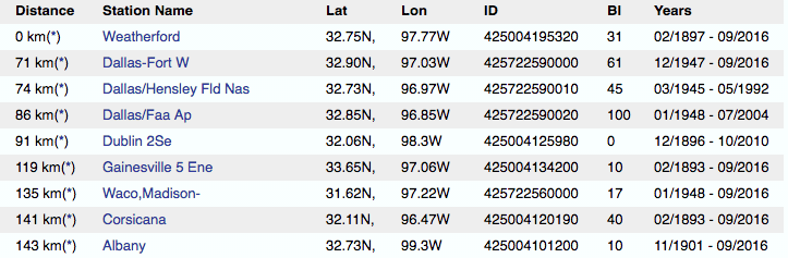
Some of them go back to the 1890s, and some to the 1940s, and one to 1901:
The screen grab:
comment image

The whole posting, from 2016:
https://realclimatescience.com/2016/10/more-noaa-texas-fraud/

Editor
January 25, 2019 7:31 am

Just to be clear: Because the reasons for measuring temperatures, in Climate Science, is use temperatures as a proxy for “energy retained in the climate system”; then Stokes’ “All this speculation about aliasing only matters when you want to make some quantitative statement that depends on what he was doing between samples.”

Average daily temperature, by any method, does not necessarily represent a true picture of the Temperature Profile of the day — and thus does not accurately represent a measured proxy for energy.

If we are trying to determine something about climate system energy — and intend to use temperatures to 1/100ths of a degree — then there may be very good reasons to use AWS 5-minute values where ever available — and to use proper error bars for all Min/Max averages.

Reply to  Kip Hansen
January 25, 2019 8:14 am

Kip,
“and thus does not accurately represent a measured proxy for energy”
Temperature is just temperature. It’s actually a potential; it tells how fast energy can be transferred across a given resistance (eg skin). It isn’t being used as a proxy for energy.

Ian W
Reply to  Nick Stokes
January 25, 2019 8:47 am

Given that it is atmospheric temperature that is being measured, the failure to actually calculate enthalpy and convert the measure to kilojoules per kilogram shows that nobody is really serious about measuring energy content.

Editor
Reply to  Nick Stokes
January 25, 2019 10:32 am

Nick ==> If you think there is some different reason in Climate Science to track average temperature and repeatedly shout “It’s the hottest year ever!” — I’d love to hear it.

Of course, tourist destinations have a use for average MONTHLY TEMPERATURES across time, but they need Average Daytime Temperature, so the tourists know what type of clothes to bring and what outdoor trivialities might be expected. Farmers and other agriculturists need a god idea of Min and Max temperatures at different times of the year, averaged for years, as well as accurate seasonal forecasts of these — accurate “last frost” dates etc.

Climate science (the real kind) needs good records of Min and Max temperatures, along with a lot of other data, to make Koppen Climate maps.

There are no legitimate reasons for anyone to be calculating Global Average Surface Temperatures (LOTI or otherwise). There is simply no scientific use for the calculated (and very approximate) GAST.

There are some legitimate use for tracking changing climatic conditions in various regions — and for air temperatures, the Minimum and Maximum temperatures, presented as time series (graphs) are more informative, even monthly averages of these can give useful information. But a single number for “monthly average temperature” is useless for any conceivable application.

If GAST is NOT being used as a proxy for energy retained in the climate system, why then is it tracked at all? (other than the obvious propaganda value for the CAGW theorists).
More appropriate are “heating degree days” and “cooling degree days” — for cities and regions.

Clyde Spencer
Reply to  Nick Stokes
January 25, 2019 11:01 am

Nick
You said, ” It [temperature] isn’t being used as a proxy for energy.” Funny, I thought that the recent articles on OHC rising more rapidly than expected were based on temperature measurements.

Reply to  Clyde Spencer
January 25, 2019 11:45 pm

Clyde,
“the recent articles on OHC rising more rapidly than expected were based on temperature measurement”
Well, the recent article by Roy Spencer included a complaint that they had expressed OHC rise as energy rather than temperature.

There are two relevant laws here;
change in heat content = ∫ρcₚ ΔT dV, ρ density cₚ specific heat capacity
and Fourier’s Law
heat flux = – k∇T

The first is what is used for ocean heat. The temperature is very variably distributed, but heat is a conserved quantity, so it makes sense to add it all up. But there isn’t a temperature associated to the whole ocean that is going to be applied to heating any particular thing.

Surface air temperature is significant because it surrounds us, and determines the rate at which heat is transferred to or from us. That’s why it has been measured and talked about for centuries (Fear no more the heat o’ the sun). And the average surface temperature is just a measure of the extent to which we and the things we care about are getting heated and cooled (the Fourier aspect). It isn’t trying to determine the heat content of something.

Editor
Reply to  Nick Stokes
January 26, 2019 8:18 am

Nick ==> You state:
“Surface air temperature is significant because it surrounds us, and determines the rate at which heat is transferred to or from us. That’s why it has been measured and talked about for centuries (Fear no more the heat o’ the sun). And the average surface temperature is just a measure of the extent to which we and the things we care about are getting heated and cooled (the Fourier aspect). It isn’t trying to determine the heat content of something.”

I am afraid I agree with you about why we track temperatures! Not so much as to why we track average temperatures….

That being the case, though, then there is no real reason for Climate Science to be tracking Global Average Surface Temperature … and certainly no reason whatever for alarm or concern over the pleasant fact that that metric has increased by one point whatever degrees since the 1880s….

Clyde Spencer
Reply to  Nick Stokes
January 26, 2019 9:39 am

Stokes
Your remark “Well, the recent article by Roy Spencer included a complaint that they had expressed OHC rise as energy rather than temperature’ is a Red Herring. I claimed that temperature was used as a proxy to calculate energy, and you confirmed it with the integral, although you tried to deflect the fact. This is why I have accused you of sophistry in the past.

Menicholas
Reply to  Nick Stokes
January 27, 2019 4:50 pm

If the real purpose is to determine how fast and by how much the air is heating or cooling our bodies, then one ought to be using data which takes into account wind, altitude and humidity.
Humid air has far more energy in it, than dry air at the same temp, and so it impedes our bodies ability to cool itself.
Windy air has more energy too, but it cools us better.
90 F is hot as hell in Florida in Summer, but not bad at all in Las Vegas when the humidity is low.

Greg
Reply to  Nick Stokes
January 25, 2019 11:45 am

It isn’t being used as a proxy for energy.

I have the greatest respect for Nick technically but if he thinks temperature is not being used ( incorrectly ) as a proxy for energy I don’t know where he has been for the last 20 years.

UN targets which are the centre of a global effort for reshape human society and energy use are expressed as temperature increase, be it 2 deg. C or the new “it would be really good to stay well under 2.0 , ie 1.5 for example” target.

All this is allegedly to be remedied by a “carbon free” future on the basis that the radiative forcing of CO2 is the primary problem.

In short you have a power term ( rate of change of energy ) being used to achieve a temperature target. They argument is about what “climate sensitivity” to the CO2 radiative forcing is , measured in the degree C per double of CO2, ie W/m^2/kelvin.

Assessing the danger and the effectiveness of any mitigation is being measured as temperature change. Quite clearly temperature is being ( albeit incorrectly ) being used as a proxy for energy.

The mindless mixing and averaging of land and sea temperatures betrays a total lack of respect for the laws of physics in the so-called scientific “debate”.

Charlie
Reply to  Nick Stokes
January 25, 2019 12:25 pm

Regards Nick,

T_max and T_min data sets are convenient, as you say there is a lot of daily temp data in that format.

T_average = the sum of these two divided by 2 (for that day). So maybe daily samples at 3 am and say, 3 pm for example.

But what if T_average from above is not close to equal to a series of say, 30 minute interval measurements of air temperature divided by 48 (for that day); T_average_high_res

This would be the result whenever the actual air temp excursions where not symmetrical in shape about the average (T_average). This could be seen from a plot for a more highly sampled set of ground temperature data, and then better reflect how much heat is actually in the air (energy) over the 24 hour period.

What if, for instance, the temp rapidly shot up to the max on a clear sunny day at 3pm, but then subsided to where it stayed close to the min for 4-6 hours that evening. The weight given to the max in this case is too high, as it does not reflect the energy content over the 24 hour period. Same in the reverse case.

Weather fronts and the location of the country (US) and prevailing winds and time of year and highs and lows and how they move will effect dwell times close to the daily T_max and T_min, and these are being missed with two samples a day.

A daily average temperature is useful, but how it is currently developed is not accurate enough to be used to change the course of human history (forward in time from now).

You could say that over many many data sets, in developing the daily average temperature term, the effect I’m taking about is a wash, and it itself averages out to the truth too. I’m not sure it would.

Ian W
Reply to  Charlie
January 25, 2019 1:04 pm

Charlie,
As pointed out later in the thread
(https://wattsupwiththat.com/2019/01/25/nyquist-sampling-anomalies-and-all-that/#comment-2604279 ),
temperature changes seem to be higher minimums more than higher maximums. It is therefore convenient to use the mathematical mean of Tmax and Tmin and claim incorrectly that ‘the temperature is rising’ It is not – the temperature is not cooling as much. This incorrect claim is then exacerbated by adding the ‘increase in mathematical mean of Tmax and Tmin’ to the Tmax figures and projecting that ‘increase’ forward.

I do not expect climate ‘scientists’ to change to a more accurate kilojoules per kilogram measured every hour which would provide a metric of atmospheric energy content, as the ‘trick’ with the temperature mean is too convenient and the gullibles press and politicians know no better so funding for climate ‘science’ is maintained.

Clyde Spencer
Reply to  Ian W
January 25, 2019 8:31 pm

Ian W
You said, “It is therefore convenient to use the mathematical mean of Tmax and Tmin and claim INCORRECTLY that ‘the temperature is rising’ It is not – the temperature is not cooling as much.”

That is why Tmin and Tmax should be tracked and displayed separately!

leitmotif
January 25, 2019 7:33 am

Where would the global warming industry be without thermometers? Is there anything they can’t do?

knr
Reply to  leitmotif
January 25, 2019 7:37 am

Modles are way , way better

January 25, 2019 7:33 am

Nice job Nick, needs the font for the equations adjusted as mentioned above. I liked the analogy with the running track, although as a 400m sprinter I would hate to race on a circular track like that one!

Jaap Titulaer
January 25, 2019 7:35 am

So in a way, fussing about regular sample rates of a few per day is theoretical only. The way it was done for centuries of records is not periodic sampling, and for modern technology, much greater sample rates are easily achieved.

Hmm. I remember distinctly reading that in quite a number of European states (German states, Russia, Scandinavia) the approach varied (certainly in the 19th century and early 20th) and one big difference was between Min/Max versus X-times At Same Time sampling.
Didn’t some sample three times per day and on a fixed schedule?

Ric (above : https://wattsupwiththat.com/2019/01/25/nyquist-sampling-anomalies-and-all-that/#comment-2604173) gives an example from NH, USA.
“temperature records were logged at 6:00 AM, 1:00 PM, and 9:00 PM each day”

And a comment about this (in Ric’s post): “Clearly people were trying to avoid the extremes at dawn and after noon.”. One should know that most information is contained in the temperature at night and during the day and that the in between moment where a switch takes place have less information.
That means that when you only sample in the middle of the night, or at some fixed time at night, say 21:00 or (better) 24:00, and you sample in the middle of the day, say 12:00 or 13:00, then you get a good profile for the typical temperature of that day.

Reply to  Jaap Titulaer
January 25, 2019 11:33 pm

Yes, people did also do readings at fixed times. In Australia, 9am and 3pm was a common schedule, and there are still quite a lot of places reporting that way. But for whatever reason, there are AFAIK no large collections of this data.

knr
January 25, 2019 7:36 am

Even if you make the casue for Min/max, you still need to considered accuracy and range of coverage , and deal with the ideas that an airport is good as it’s the same type of environment has the rest of the area it is supposed to cover.
It’s fair to ask has about ability to make such measurements in this area , really improved at all from before the days of ‘settled science’ and weather forecasts of an accuracy of ‘in the summer it is warming than in winter ‘ for more than 72 hours head?

Ian W
January 25, 2019 7:42 am

My problem with the sparse sampling is that it seems to be that it is the arithmetic mean of the maximum temperature and minimum temperature that is calculated and called an ‘average temperature’ – which is incorrect. Then that figure is used as the ‘average temperature’ for the day. This means that if the minimums are getting higher but the maximums are remaining the same, their arithmetic mean will be higher. This is then trumpeted as a temperature increase, when in fact it is a reduced decrease. The false temperature increases are then averaged again and projected into the future as a rate of ‘temperature increase’ and the oceans will boil .. Whereas what is really happening is that the cooling rate has slowed but the top temperatures may have remained constant, or even cooled.

Have I misconstrued the way the daily temperature observations are ‘averaged’ and their subsequent incorrect use?

Jaap Titulaer
Reply to  Ian W
January 25, 2019 8:05 am

I don’t think so.

To calculate a reasonable average (as opposed to mode or some other semi-average) one needs to determine a reasonable estimate for each hour of the day.

Assuming that the minimum is representative for the night is a bit dangerous (as it is too low vs the average nightly temperature). Same with assuming that the maximum fairly represents the daytime.
Otherwise when you have a representative measurement for nightly temperatures and a representative measurement for daytime temperatures you can get a reasonable estimate for the entire day by determining the number of hours to be assumed to be ‘day’ vs ‘night’ for that calendar date at that location. Based on that you can then calculate a reasonable estimate.
And that will clearly differ from (min+max)/2

Say dawn is at 8:00 and dusk is at 18:00 on a given day for a given location. Then we have 10 daylight hours and 14 hours of night. Of course we have two switch moments.
Night (prev): -1 C
Dawn
Day: 9.5 C
Dusk
Night: -2 C
When we ignore the switch moments then we get an average of (10*9.5 + 14*-2)/24= 2.8 C
The (min+max)/2 = (-2+9.5)/2=7.5/2= 3.8 C
Clearly a big difference.

When we assume Dusk and Dawn are switch moment of about 1 hr the answer is similar. The difference is that in order to estimate Dawn (we only know night & day) we need to use the temperature of the previous night.

What is more important though is consistency and knowing what the number represents.

Ian W
Reply to  Jaap Titulaer
January 25, 2019 8:53 am

The real problem is that a increase in just the minimum temperature increases the mean, and that is claimed to be a ‘rise in average temperatures’ which is incorrect. It is a reduction in cooling. This is then exacerbated by adding the change in mean to the top temperature for projections forward of expected anomalies.

What should happen is that the minimums should be averaged and the maximums averaged separately. Judging by several reports from different countries, this would actually show a continual decrease in maximum temperatures and a continual increase in minimum temperatures.

For that reason I do not expect anything to be changed as the entire hypothesis would be falsified and lots of careers and funds would be lost.

steve case
Reply to  Ian W
January 25, 2019 9:15 am

Ian W January 25, 2019 at 8:53 am
BINGO!
Yes, why aren’t the Min and Max tracked?

The IPCC tells us that the warming is at night, in winter, and in the Arctic.
Afternoons, summers and the tropics, not so much.

Yes summers are cooling at least in the United States (48) they are:
comment image

Clyde Spencer
Reply to  Ian W
January 25, 2019 10:56 am

Ian W
+1

Jaap Titulaer
Reply to  Ian W
January 25, 2019 12:48 pm

Exactly. Also a (perhaps spiked) minimum does not really give a good impression of the (average, typical) night temperature. Same for a maximum.
And (min+max)/2 is not a proper average.
These are best tracked separately as these are different things. If you wish by using an anomaly (one for min and the other for max).

Reply to  Ian W
January 25, 2019 6:03 pm

Excellent comment. Isn’t it odd that C02 can increase the minimum temperatures but not affect the higher temperatures, unless of course those higher temperatures are recorded in a large metropolitan area.

Editor
January 25, 2019 7:50 am

Well done Nick. Very good explanation of Nyquist.

While I think the principles of signal processing are routinely violated in climate reconstructions and Nyquist is a very significant factor in ice and sediment core data, I tend to think you are right about its relationship to min/max temperature readings.

RicDre
January 25, 2019 7:52 am

Mr. Stokes:

Thank you for posting this article.

steve case
January 25, 2019 7:56 am

“Nyquist, sampling, anomalies and all that”
(Or 2,000 words on finding the average daily
temperature for a single weather station.)

Beware of averages. The average person has one breast and one testicle. Dixie Lee Ray

First we find the station average for the day (The 2,000 words). Then using that average we find the average for the year. Then taking that annual average for all the stations from the equator to the poles we average all those up to get the annual global temperature. Finally all those yearly temperatures are plotted out to see if there’s a trend or not, and if there is, it is declared that it’s an artifact of human activity and a problem. The solution to the “problem” requires that we all have to eat tofu, ride the bus and show up at the euthanization center on our 65th birthday to save the planet.

John Tillman
Reply to  steve case
January 25, 2019 8:14 am

The outspoken Dixy Lee Ray said that during a 1991 speech in Pasco, WA, denouncing “climate change” foolishness.

Greg
Reply to  steve case
January 25, 2019 2:05 pm

The average person has one breast and one testicle. Dixie Lee Ray

I like that one, I’ll take a note. However, I think you need error bars. At least in the West, the average person has slightly less than one testicle , I believe.

Alasdair
January 25, 2019 8:06 am

I am a bit diffident about my comments here as I have only grasped the gist of this post.
However in the back of my mind I ask: What is the point of this?
To me the result of whatever measuring/statistical methods are employed leaves open the question of: What does this mean and what value does it have?
It is a matter of CONSISTENCY if anomalies and trends are to be considered, not the methods themselves. The methods merely add value to the results whatever interpretation be put on this value.

Today consistency of measurement is more in the intent rather than the reality and similarly the statistical analysis methods vary; so more or less all conclusions or conjectures are suspect or open to question.

The concept of Global Temperature is, in itself a questionable matter if you wish to define it.; for it raises immediately the circular question: Well how is it to be measured?
As far as Nick Stokes’s erudite post is concerned there does seem to be a case to include the Nuquist methods into the statistics ; but only if it is consistently used along with the actual and consistent measurement data.

As an aside: In spite of all I have seen on matters of global temperature my old thermometer seems to have totally flatlined oblivious of the anomalies! Mind you I am hardly consistent in the observations! Meanwhile my bones tell me that there has been a bit of welcome warming over the years.

Phoenix44
January 25, 2019 8:10 am

Bit disingenuous. We may well have been using min/max for many decades, but we haven’t been using min/max to show that we must fundamentally change our economy for all that time. If all this were just an academic exercise I couldn’t’t care less (except about the debasement of scicience) but it is not.

vukcevic
January 25, 2019 8:31 am

Let’s assume that lunar tides have some subtle effect on surface temperature via the ‘nearly’ diurnal cycle of expansion of atmosphere, or simply on the ocean currents velocity. Since the lunar cycles are not in sync with the earth’s rotating or orbital periodicity the effect would be aliasing on monthly, annual, multi decadadal and centenary time scales, following changes in intensity of the lunar tides across the time scales mentioned. Just using two simple periodicity of 27.3 and 365.25 days produces some of the familiar spectral components found in the global temperature anomaly.

Ben Vorlich
Reply to  vukcevic
January 25, 2019 10:06 am

Don’t forget the 19 year Metonic cycle used by the Babylonians.

Steve O
January 25, 2019 8:37 am

All this discussion on whether or not the sampling method is adequate or not can be resolved by running simulations. You can create a dataset that represents a true continual temperature trend over the course of 10 years . You can calculate the value for the “actual” average temperature over different periods of time, and compare that to the values you get from various sampling methods.

I suspect that anyone who does such an experiment will find that developing a metric by taking 365 sets of readings in a year, recording the Tmin and TMax (rounded to the nearest whole numbers), and dividing by two, is adequate to determine the actual average annual temperature and that it’s good enough to be able to discern trends in the underlying data.

wsbriggs
January 25, 2019 8:45 am

I’m somewhat frustrated by the whole min/max thing anyway. Living in E. Texas I get to experience “exceptional” weather if not weekly, certainly monthly. In the Winter we have cold fronts which stall just to the south, over the Gulf, and having brought cooler weather, then reverse, become warm fronts, switch the winds again and warm us up. Not infrequently the fronts are fast moving and drop the temperatures 30+ F/13 C in less than an hour. Now we get the min/max temperature reading whenever, but almost assuredly not on some arbitrary data input time. The old min/max thermometer can tell you what, but not when, and two samples a day aren’t accurate either unless they just happened to fall at the right time. Since most two sample protocols have the times defined, one is almost guaranteed to have the wrong values recorded.

One might say that in some areas the temperature curve is an arbitrary, continuous shape. To map the shape half way accurately one needs more than 24 samples a day, but sampling every second is probably overkill.

In any case, whether in UHI, or in the boonies, you live the weather that is there, not the weather that’s recorded.

Greg
Reply to  wsbriggs
January 25, 2019 2:15 pm

Since most two sample protocols have the times defined, one is almost guaranteed to have the wrong values recorded.

Why would that be “wrong”. What are you aiming to achieve and in what way would a protocol with specific times be “correct”?

There is no specific time of day for minimum temperature. If you specify a time the result could vary considerably. In what way would a fixed time reading be “right”?

Marcus
January 25, 2019 9:14 am

Averaging min/max temps makes no sense. What if it is cloudy from 6am till 1pm(cooler), then cloudless till 2pm,(warmer), then cloudy again till 6am the next day . Your max would be from 1 hour of warmer and your min from 23 hours of cooler ?

Steve O
Reply to  Marcus
January 25, 2019 10:07 am

On average, the result would be average.

Gator
Reply to  Steve O
January 25, 2019 10:51 am

On the vast majority of days, one never encounters an average high or average low temperature. Averages are a construct of man, and not nature, they mean nothing to Gaia. Averages are a fantasy.

Alan Tomalty
January 25, 2019 9:33 am

In any case, temperature measuring can not prove and separate out the difference between natural warming and man made. Our politicians have simply assumed that any temperature increase has been due to AGW. They have been aided and abetted by the devious climate scientists that have refused to use the Null hypothesis testing in any of their reports. Thayer Watkins has said that 85 % of all LWIR back radiation is due to clouds. NASA says 50%. I have shown that NASA must be wrong on this point and I have demonstrated the maximum effect of CO2 on temperature increase, assuming that we have even had a temperature increase in last 68 years.

http://applet-magic.com/cloudblanket.htm
Clouds overwhelm the Downward Infrared Radiation (DWIR) produced by CO2. At night with and without clouds, the temperature difference can be as much as 11C. The amount of warming provided by DWIR from CO2 is negligible but is a real quantity. We give this as the average amount of DWIR due to CO2 and H2O or some other cause of the DWIR. Now we can convert it to a temperature increase and call this Tcdiox.The pyrgeometers assume emission coeff of 1 for CO2. CO2 is NOT a blackbody. Clouds contribute 85% of the DWIR. GHG’s contribute 15%. See the analysis in link. The IR that hits clouds does not get absorbed. Instead it gets reflected. When IR gets absorbed by GHG’s it gets reemitted either on its own or via collisions with N2 and O2. In both cases, the emitted IR is weaker than the absorbed IR. Don’t forget that the IR from reradiated CO2 is emitted in all directions. Therefore a little less than 50% of the absorbed IR by the CO2 gets reemitted downward to the earth surface. Since CO2 is not transitory like clouds or water vapour, it remains well mixed at all times. Therefore since the earth is always giving off IR (probably a maximum at 5 pm everyday), the so called greenhouse effect (not really but the term is always used) is always present and there will always be some backward downward IR from the atmosphere.

When there isn’t clouds, there is still DWIR which causes a slight warming. We have an indication of what this is because of the measured temperature increase of 0.65 from 1950 to 2018. This slight warming is for reasons other than just clouds, therefore it is happening all the time. Therefore in a particular night that has the maximum effect , you have 11 C + Tcdiox. We can put a number to Tcdiox. It may change over the years as CO2 increases in the atmosphere. At the present time with 409 ppm CO2, the global temperature is now 0.65 C higher than it was in 1950, the year when mankind started to put significant amounts of CO2 into the air. So at a maximum Tcdiox = 0.65C. We don’t know the exact cause of Tcdiox whether it is all H2O caused or both H2O and CO2 or the sun or something else but we do know the rate of warming. This analysis will assume that CO2 and H2O are the only possible causes. That assumption will pacify the alarmists because they say there is no other cause worth mentioning. They like to forget about water vapour but in any average local temperature calculation you can’t forget about water vapour unless it is a desert. A proper calculation of the mean physical temperature of a spherical body requires an explicit integration of the Stefan-Boltzmann equation over the entire planet surface. This means first taking the 4th root of the absorbed solar flux at every point on the planet and then doing the same thing for the outgoing flux at Top of atmosphere from each of these points that you measured from the solar side and subtract each point flux and then turn each point result into a temperature field by integrating over the whole earth and then average the resulting temperature field across the entire globe. This gets around the Holder inequality problem when calculating temperatures from fluxes on a global spherical body. However in this analysis we are simply taking averages applied to one local situation because we are not after the exact effect of CO2 but only its maximum effect. In any case Tcdiox represents the real temperature increase over last 68 years. You have to add Tcdiox to the overall temp difference of 11 to get the maximum temperature difference of clouds, H2O and CO2 . So the maximum effect of any temperature changes caused by clouds, water vapour, or CO2 on a cloudy night is 11.65C. We will ignore methane and any other GHG except water vapour.

So from the above URL link clouds represent 85% of the total temperature effect , so clouds have a maximum temperature effect of .85 * 11.65 C = 9.90 C. That leaves 1.75 C for the water vapour and CO2. This is split up with 60% for water vapour and 26% for CO2 with the remaining % for methane, ozone ….etc. See the study by Ahilleas Maurellis and Jonathan Tennyson May 2003 in Physics World. Amazingly this is the only study that quantifies the Global warming potential of H20 before any feedback effects. CO2 will have relatively more of an effect in deserts than it will in wet areas but still can never go beyond this 1.75 C . Since the desert areas are 33% of 30% (land vs oceans) = 10% of earth’s surface , then the CO2 has a maximum effect of 10% of 1.75 + 90% of Twet. We define Twet as the CO2 temperature effect of over all the world’s oceans and the non desert areas of land. There is an argument for less IR being radiated from the world’s oceans than from land but we will ignore that for the purpose of maximizing the effect of CO2 to keep the alarmists happy for now. So CO2 has a maximum effect of 0.175 C + (.9 * Twet). So all we have to do is calculate Twet.

Reflected IR from clouds is not weaker. Water vapour is in the air and in clouds. Even without clouds, water vapour is in the air. No one knows the ratio of the amount of water vapour that has now condensed to water/ice in the clouds compared to the total amount of water vapour/H2O in the atmosphere but the ratio can’t be very large. Even though clouds cover on average 60 % of the lower layers of the troposhere, since the troposphere is approximately 8.14 x 10^18 m^3 in volume, the total cloud volume in relation must be small. Certainly not more than 5%. H2O is a GHG. So of the original 15% contribution by GHG’s of the DWIR, we have .15 x .26 =0.039 or 3.9% to account for CO2. Now we have to apply an adjustment factor to account for the fact that some water vapour at any one time is condensed into the clouds. So add 5% onto the 0.039 and we get 0.041 or 4.1 % . CO2 therefore contributes 4.1 % of the DWIR in non deserts. We will neglect the fact that the IR emitted downward from the CO2 is a little weaker than the IR that is reflected by the clouds. Since, as in the above, a cloudy night can make the temperature 11C warmer than a clear sky night, CO2 or Twet contributes a maximum of 0.041 * 1.75 C = 0.07 C.
Therfore Since Twet = 0.07 C we have in the above equation CO2 max effect = 0.175 C + (.9 * 0.07 C ) = ~ 0.238 C. As I said before; this will increase as the level of CO2 increases, but we have had 68 years of heavy fossil fuel burning and this is the absolute maximum of the effect of CO2 on global temperature.

So how would any average global temperature increase by 7C or even 2C, if the maximum temperature warming effect of CO2 today from DWIR is only 0.238 C? This means that the effect of clouds = 85%, the effect of water vapour = 13 % and the effect of CO2 = 2 %. Sure, if we quadruple the CO2 in the air which at the present rate of increase would take 278 years, we would increase the effect of CO2 (if it is a linear effect) to 4 X 0.238 C = 0.952 C .

If the cloud effect was 0 for DWIR, the maximum that CO2 could be is 10%(desert) * 0.65 + (90% of Twet2) = 0.065 C + (90% *twet2)

twet2 = .26( See the study by Ahilleas Maurellis and Jonathan Tennyson May 2003 in Physics World.) * 0.585 C (difference between 0.65 and the amount of temperature effect for CO2 for desert) = 0.1521 C therefore Max CO2 = 0.065 C + (0.1521 * .9) = 0.2 C ((which is about 84% of above figure of 0.238 C. The 0.2 C was calculated by assuming as above that on average H20 is 60% of greenhouse effect and CO2 is 26% of GHG effect and that the whole change of 0.65 C from 1950 to 2018 is because of either CO2 or water vapour. We are disregarding methane and ozone. So in effect, the above analysis regarding clouds gave too much maximum effect to CO2. The reason is that you simply take the temperature change from 1950 to 2018 disregarding clouds, since the water vapour has 60% of the greenhouse effect and CO2 has 26%. If you integrate the absorption flux across the IR spectrum despite the fact that there are 25 times more molecules than CO2 by volume, you get 60% for H20 and 26% for CO2 as their GHG effects. See the study by Ahilleas Maurellis and Jonathan Tennyson May 2003 in Physics World. CO2 can never have as much effect as H20 until we get to 2.3x the amount of CO2 in the atmosphere than there is now.

NASA says clouds have only a 50% effect on DWIR. So let us do that analysis.

So according to NASA clouds have a maximum temperature effect of .5 * 11.65 C = 5.825 C. That leaves 5.825 C for the water vapour and CO2. This is split up with 60% for water vapour and 26% for CO2 with the remaining % for methane, ozone ….etc. As per the above. Again since the desert areas are 33% of 30% (land vs oceans) = 10% of earth’s surface , then the CO2 has a maximum effect of (10% of 5.825 C) + 90% of TwetNASA. We define TwetNASA as the CO2 temperature effect of over all the world’s oceans and the non desert areas of land. So CO2 has a maximum effect of 0.5825 C + (.9 * TwetNASA). So all we have to do is calculate TwetNASA.
Since as before we give the total cloud volume in relation to the whole atmosphere as not more than 5%. H2O is a GHG. So of the original 50% contribution by GHG’s of the DWIR, we have .5 x .26 =0.13 or 13 % to account for CO2. Now we have to apply an adjustment factor to account for the fact that some water vapour at any one time is condensed into the clouds. So add 5% onto the 0.13 and we get 0.1365 or 13.65 % . CO2 therefore contributes 13.65 % of the DWIR in non deserts. As before, we will neglect the fact that the IR emitted downward from the CO2 is a little weaker than the IR that is reflected by the clouds.

Since, as in the above, a cloudy night can make the temperature 11C warmer than a clear sky night, CO2 or TwetNASA contributes a maximum of 0.1365 * 5.825 C = ~0.795 C.
Therfore Since TwetNASA = 0.795 C we have in the above equation CO2 max effect = 0.5825 C + (.9 * 0.795 C ) = ~ 1.3 C. Now this is double the amount of actual global warming in the last 68 years, so since CO2 would not have more of an effect on a cloudy night versus a noncloudy night, the maximum effect could not be greater than the effect calculated, above, when not considering clouds. So clearly, NASA cannot be correct.
I fail to understand how climate scientists could get away with saying that water vapour doesnt matter because it is transitory. In fact the alarmist theory needs a positive forcing of water vapour to achieve CAGW heat effects. Since there is widespread disagreement on any increase in H2O in the atmosphere in the last 68 years, there hasn’t been any positive forcing so far. Therefore; the hypothesis is; that main stream climate science theory of net CO2 increases in the atmosphere has major or catastrophic consequences for heating the atmosphere and the null hypothesis says it doesn’t have major or catastrophic consequences for heating the atmosphere. Therefore we must conclude that we cannot reject the null hypothesis that main stream climate science theory of net CO2 increases in the atmosphere does not have major or catastrophic consequences for heating the atmosphere. In fact the evidence and the physics of the atmosphere shows that if we rejected the null hypothesis, we would be rejecting most of radiative atmospheric physics as we know it. So in the end, the IPCC conclusion of mankind increasing net CO2 into the atmosphere, causing major or catastrophic warming of the atmosphere; is junk science.

Alan Tomalty
Reply to  Alan Tomalty
January 25, 2019 10:12 am

Please disregard the above post and substitute the following analysis of the maximum temperature effect of clouds and CO2.

http://applet-magic.com/cloudblanket.htm
Clouds overwhelm the Downward Infrared Radiation (DWIR) produced by CO2. At night with and without clouds, the temperature difference can be as much as 11C. The amount of warming provided by DWIR from CO2 is negligible but is a real quantity. We give this as the average amount of DWIR due to CO2 and H2O or some other cause of the DWIR. Now we can convert it to a temperature increase and call this Tcdiox.The pyrgeometers assume emission coeff of 1 for CO2. CO2 is NOT a blackbody. Clouds contribute 85% of the DWIR. GHG’s contribute 15%. See the analysis in link. The IR that hits clouds does not get absorbed. Instead it gets reflected. When IR gets absorbed by GHG’s it gets reemitted either on its own or via collisions with N2 and O2. In both cases, the emitted IR is weaker than the absorbed IR. Don’t forget that the IR from reradiated CO2 is emitted in all directions. Therefore a little less than 50% of the absorbed IR by the CO2 gets reemitted downward to the earth surface. Since CO2 is not transitory like clouds or water vapour, it remains well mixed at all times. Therefore since the earth is always giving off IR (probably a maximum at 5 pm everyday), the so called greenhouse effect (not really but the term is always used) is always present and there will always be some backward downward IR from the atmosphere.

When there isn’t clouds, there is still DWIR which causes a slight warming. We have an indication of what this is because of the measured temperature increase of 0.65 from 1950 to 2018. This slight warming is for reasons other than just clouds, therefore it is happening all the time. Therefore in a particular night that has the maximum effect , you have 11 C + Tcdiox. We can put a number to Tcdiox. It may change over the years as CO2 increases in the atmosphere. At the present time with 411 ppm CO2, the global temperature is now 0.65 C higher than it was in 1950, the year when mankind started to put significant amounts of CO2 into the air. So at a maximum Tcdiox = 0.65C. We don’t know the exact cause of Tcdiox whether it is all H2O caused or both H2O and CO2 or the sun or something else but we do know the rate of warming. This analysis will assume that CO2 and H2O are the only possible causes. That assumption will pacify the alarmists because they say there is no other cause worth mentioning. They like to forget about water vapour but in any average local temperature calculation you can’t forget about water vapour unless it is a desert. A proper calculation of the mean physical temperature of a spherical body requires an explicit integration of the Stefan-Boltzmann equation over the entire planet surface. This means first taking the 4th root of the absorbed solar flux at every point on the planet and then doing the same thing for the outgoing flux at Top of atmosphere from each of these points that you measured from the solar side and subtract each point flux and then turn each point result into a temperature field by integrating over the whole earth and then average the resulting temperature field across the entire globe. This gets around the Holder inequality problem when calculating temperatures from fluxes on a global spherical body. However in this analysis we are simply taking averages applied to one local situation because we are not after the exact effect of CO2 but only its maximum effect. In any case Tcdiox represents the real temperature increase over last 68 years. You have to add Tcdiox to the overall temp difference of 11 to get the maximum temperature difference of clouds, H2O and CO2 . So the maximum effect of any temperature changes caused by clouds, water vapour, or CO2 on a cloudy night is 11.65C. We will ignore methane and any other GHG except water vapour.

So from the above URL link clouds represent 85% of the total temperature effect , so clouds have a maximum temperature effect of .85 * 11.65 C = 9.90 C. That leaves 1.75 C for the water vapour and CO2. This is split up with 60% for water vapour and 26% for CO2 with the remaining % for methane, ozone ….etc. See the study by Ahilleas Maurellis and Jonathan Tennyson May 2003 in Physics World. Amazingly this is the only study that quantifies the Global warming potential of H20 before any feedback effects. CO2 will have relatively more of an effect in deserts than it will in wet areas but still can never go beyond this 1.75 C . Since the desert areas are 33% of 30% (land vs oceans) = 10% of earth’s surface , then the CO2 has a maximum effect of 10% of 1.75 + 90% of Twet. We define Twet as the CO2 temperature effect of over all the world’s oceans and the non desert areas of land. There is an argument for less IR being radiated from the world’s oceans than from land but we will ignore that for the purpose of maximizing the effect of CO2 to keep the alarmists happy for now. So CO2 has a maximum effect of 0.175 C + (.9 * Twet). So all we have to do is calculate Twet.

Reflected IR from clouds is not weaker. Water vapour is in the air and in clouds. Even without clouds, water vapour is in the air. No one knows the ratio of the amount of water vapour that has now condensed to water/ice in the clouds compared to the total amount of water vapour/H2O in the atmosphere but the ratio can’t be very large. Even though clouds cover on average 60 % of the lower layers of the troposhere, since the troposphere is approximately 8.14 x 10^18 m^3 in volume, the total cloud volume in relation must be small. Certainly not more than 5%. H2O is a GHG. So of the original 15% contribution by GHG’s of the DWIR, we have .15 x .26 =0.039 or 3.9% to account for CO2. Now we have to apply an adjustment factor to account for the fact that some water vapour at any one time is condensed into the clouds. So add 5% onto the 0.039 and we get 0.041 or 4.1 % . CO2 therefore contributes 4.1 % of the DWIR in non deserts. We will neglect the fact that the IR emitted downward from the CO2 is a little weaker than the IR that is reflected by the clouds. Since, as in the above, a cloudy night can make the temperature 11C warmer than a clear sky night, CO2 or Twet contributes a maximum of 0.041 * 1.75 C = 0.07 C.
Therfore Since Twet = 0.07 C we have in the above equation CO2 max effect = 0.175 C + (.9 * 0.07 C ) = ~ 0.238 C. As I said before; this will increase as the level of CO2 increases, but we have had 68 years of heavy fossil fuel burning and this is the absolute maximum of the effect of CO2 on global temperature.

So how would any average global temperature increase by 7C or even 2C, if the maximum temperature warming effect of CO2 today from DWIR is only 0.238 C? This means that the effect of clouds = 85%, the effect of water vapour = 13 % and the effect of CO2 = 2 %. Sure, if we quadruple the CO2 in the air which at the present rate of increase would take 278 years, we would increase the effect of CO2 (if it is a linear effect) to 4 X 0.238 C = 0.952 C .

If the cloud effect was 0 for DWIR, the maximum that CO2 could be is 10%(desert) * 0.65 + (90% of Twet2) = 0.065 C + (90% *twet2)

twet2 = .26( See the study by Ahilleas Maurellis and Jonathan Tennyson May 2003 in Physics World.) * 0.585 C (difference between 0.65 and the amount of temperature effect for CO2 for desert) = 0.1521 C therefore Max CO2 = 0.065 C + (0.1521 * .9) = 0.2 C ((which is about 84% of above figure of 0.238 C. The 0.2 C was calculated by assuming as above that on average H20 is 60% of greenhouse effect and CO2 is 26% of GHG effect and that the whole change of 0.65 C from 1950 to 2018 is because of either CO2 or water vapour. We are disregarding methane and ozone. So in effect, the above analysis regarding clouds gave too much maximum effect to CO2. The reason is that you simply take the temperature change from 1950 to 2018 disregarding clouds, since the water vapour has 60% of the greenhouse effect and CO2 has 26%. If you integrate the absorption flux across the IR spectrum despite the fact that there are 25 times more molecules than CO2 by volume, you get 60% for H20 and 26% for CO2 as their GHG effects. See the study by Ahilleas Maurellis and Jonathan Tennyson May 2003 in Physics World. CO2 can never have as much effect as H20 until we get to 2.3x the amount of CO2 in the atmosphere than there is now.

NASA says clouds have only a 50% effect on DWIR. So let us do that analysis.

So according to NASA clouds have a maximum temperature effect of .5 * 11.65 C = 5.825 C. That leaves 5.825 C for the water vapour and CO2. This is split up with 60% for water vapour and 26% for CO2 with the remaining % for methane, ozone ….etc. As per the above. Again since the desert areas are 33% of 30% (land vs oceans) = 10% of earth’s surface , then the CO2 has a maximum effect of (10% of 5.825 C) + 90% of TwetNASA. We define TwetNASA as the CO2 temperature effect of over all the world’s oceans and the non desert areas of land. So CO2 has a maximum effect of 0.5825 C + (.9 * TwetNASA). So all we have to do is calculate TwetNASA.
Since as before we give the total cloud volume in relation to the whole atmosphere as not more than 5%. H2O is a GHG. So of the original 50% contribution by GHG’s of the DWIR, we have .5 x .26 =0.13 or 13 % to account for CO2. Now we have to apply an adjustment factor to account for the fact that some water vapour at any one time is condensed into the clouds. So add 5% onto the 0.13 and we get 0.1365 or 13.65 % . CO2 therefore contributes 13.65 % of the DWIR in non deserts. As before, we will neglect the fact that the IR emitted downward from the CO2 is a little weaker than the IR that is reflected by the clouds.

Since, as in the above, a cloudy night can make the temperature 11C warmer than a clear sky night, CO2 or TwetNASA contributes a maximum of 0.1365 * 5.825 C = ~0.795 C.
Therfore Since TwetNASA = 0.795 C we have in the above equation CO2 max effect = 0.5825 C + (.9 * 0.795 C ) = ~ 1.3 C.

Now since the above analysis dealt with maximum effects let us divide the 11C maximum difference in temperature by 2 to get a rough estimate of the average effect of clouds. Therefore we have to do the calculations as per the above by substituting 5.5C wherever we see 11C.
So we have then 5.5C + 0.65C = 6.15C for the average effect of temperature difference with and without clouds.
So according to NASA clouds have a maximum temperature effect of .5 * 6.15 C = 3.075 C. That leaves 3.075 C for the water vapour and CO2. This is split up with 60% for water vapour and 26% for CO2 with the remaining % for methane, ozone ….etc. As per the above. Again since the desert areas are 33% of 30% (land vs oceans) = 10% of earth’s surface , then the CO2 has a maximum effect of (10% of 3.075 C) + 90% of TwetNASA. We define TwetNASA as the CO2 temperature effect of over all the world’s oceans and the non desert areas of land. So CO2 has a maximum effect of 0.3075 C + (.9 * TwetNASA). So all we have to do is calculate TwetNASA.
Since as before we give the total cloud volume in relation to the whole atmosphere as not more than 5%. H2O is a GHG. So of the original 50% contribution by GHG’s of the DWIR, we have .5 x .26 =0.13 or 13 % to account for CO2. Now we have to apply an adjustment factor to account for the fact that some water vapour at any one time is condensed into the clouds. So add 5% onto the 0.13 and we get 0.1365 or 13.65 % . CO2 therefore contributes 13.65 % of the DWIR in non deserts. As before, we will neglect the fact that the IR emitted downward from the CO2 is a little weaker than the IR that is reflected by the clouds.

Since, as in the above, a cloudy night can make the temperature 11C warmer than a clear sky night, CO2 or TwetNASA contributes a maximum of 0.1365 * 3.075 C = ~0.42 C.
Therfore Since TwetNASA = 0.42 C we have in the above equation CO2 max effect = 0.3075 C + (.9 * 0.42 C ) = ~ 0.6855C.

Since this temperature number is the complete temperature increase of the last 68 years, NASA is ignoring water vapour’s role which is 60% of the effect of GHGs. So clearly, NASA cannot be correct.

However let us redo the numbers with average temperature difference of 11/4 = 2.75 C between a cloudy and non cloudy day.

So we have then 2.75C + 0.65C = 3.4C for the average effect of temperature difference with and without clouds.
So according to NASA clouds have a maximum temperature effect of .5 * 3.4 C = 1.7 C. That leaves 1.7 C for the water vapour and CO2. This is split up with 60% for water vapour and 26% for CO2 with the remaining % for methane, ozone ….etc. As per the above. Again since the desert areas are 33% of 30% (land vs oceans) = 10% of earth’s surface , then the CO2 has a maximum effect of (10% of 1.7 C) + 90% of TwetNASA. We define TwetNASA as the CO2 temperature effect of over all the world’s oceans and the non desert areas of land. So CO2 has a maximum effect of 0.17 C + (.9 * TwetNASA). So all we have to do is calculate TwetNASA.
Since as before we give the total cloud volume in relation to the whole atmosphere as not more than 5%. H2O is a GHG. So of the original 50% contribution by GHG’s of the DWIR, we have .5 x .26 =0.13 or 13 % to account for CO2. Now we have to apply an adjustment factor to account for the fact that some water vapour at any one time is condensed into the clouds. So add 5% onto the 0.13 and we get 0.1365 or 13.65 % . CO2 therefore contributes 13.65 % of the DWIR in non deserts. As before, we will neglect the fact that the IR emitted downward from the CO2 is a little weaker than the IR that is reflected by the clouds.

Since, as in the above, a cloudy night can make the temperature 11C warmer than a clear sky night, CO2 or TwetNASA contributes a maximum of 0.1365 * 1.7 C = ~0.232 C.
Therfore Since TwetNASA = 0.232 C we have in the above equation CO2 max effect = 0.17 C + (.9 * 0.232 C ) = ~ 0.3788C.

As you can see the effect calculated for CO2 is still more than 50% of the actual temperature increase for the last 68 years. Clearly this is wrong since water vapour is 2.3 times the effect of CO2 as per the above study by Ahilleas Maurellis et al. So we must conclude that NASA is wrong and that the difference effect of temperature with and without clouds must be due mainly to clouds which makes intuitive sense. Thayer Watkins number must be closer to the truth than the number of NASA.

***************************************************************************************************
I fail to understand how climate scientists could get away with saying that water vapour doesnt matter because it is transitory. In fact the alarmist theory needs a positive forcing of water vapour to achieve CAGW heat effects. Since there is widespread disagreement on any increase in H2O in the atmosphere in the last 68 years, there hasn’t been any positive forcing so far. Therefore; the hypothesis is; that main stream climate science theory of net CO2 increases in the atmosphere has major or catastrophic consequences for heating the atmosphere and the null hypothesis says it doesn’t have major or catastrophic consequences for heating the atmosphere. Therefore we must conclude that we cannot reject the null hypothesis that main stream climate science theory of net CO2 increases in the atmosphere does not have major or catastrophic consequences for heating the atmosphere. In fact the evidence and the physics of the atmosphere shows that if we rejected the null hypothesis, we would be rejecting most of radiative atmospheric physics as we know it. So in the end, the IPCC conclusion of mankind increasing net CO2 into the atmosphere, causing major or catastrophic warming of the atmosphere; is junk science.

Clyde Spencer
Reply to  Alan Tomalty
January 25, 2019 11:12 am

Alan
You said, “I fail to understand how climate scientists could get away with saying that water vapour doesnt matter because it is transitory.” Any given molecule may have a short residency; however, the WV is continually replenished in the source areas. In modern times, that means evaporation from reservoirs and irrigated fields, and water produced from the combustion of hydrocarbons. These are sources that didn’t exist before modern civilization.

Anthony Banton
Reply to  Clyde Spencer
January 25, 2019 11:57 am

“In modern times, that means evaporation from reservoirs and irrigated fields, and water produced from the combustion of hydrocarbons. These are sources that didn’t exist before modern civilization.”

And is negligible at the side of feedback from GHG warming …..

“Direct emission of water vapour by human activities makes a negligible contribution to radiative forcing.
However, as global mean temperatures increase, tropospheric water vapour concentrations increase and this represents a key feedback but not a forcing of climate change. Direct emission of water to the atmosphere by anthropogenic activities, mainly irrigation, is a possible forcing factor but corresponds to less than 1% of the natural sources of atmospheric water vapour. The direct injection of water vapour into the atmosphere from fossil fuel combustion is significantly lower than that from agricultural activity. {2.5}”

https://www.ipcc.ch/site/assets/uploads/2018/02/ar4-wg1-ts-1.pdf

Jaap Titulaer
Reply to  Anthony Banton
January 25, 2019 1:07 pm

Direct emission of water vapour by human activities makes a negligible contribution to radiative forcing.

Direct emission of water to the atmosphere by anthropogenic activities, mainly irrigation, is a possible forcing factor but corresponds to less than 1% of the natural sources of atmospheric water vapour.

Unfounded claim (1st). And misleading (2nd sentence) because irrelevant.

The question is not how large the extra WV is that is produced by man via such ways as irrigation, but whether the extra WV which is thereby put into the air is larger than the extra WV that is supposed to get into the air merely because of the minute warming caused by CO2.
That minute amount of extra WV due to CO2 direct warming is supposed to give the actual total greenhouse effect (x3 or x4 the original CO2 effect).

The extra WV put into the air via land use changes and irrigation is actually quite significant. Entire sea’s (Russia) and rivers (e.g. Colorado river) are used up for irrigation. The local climate in a large part of India has changed (notably) due to irrigation and also in Kansas (10% more WV).

Irrigation (and similar water use for agriculture) has increased by a very large amount since 1950 as that was needed to keep up with population growth,

Also irrigation has become significantly less wasteful than it was in the earlier part of the 20th century. No more sprinkling on top, but feeding low to the ground via tubes. The idea that this was better is fairly new in most regions, and only introduced in many places after the 1990’s… perhaps as late as this century. So while population and agriculture output kept growing, the use of water has not rising that much since about 2000…
Get it?

Clyde Spencer
Reply to  Anthony Banton
January 25, 2019 4:49 pm

Anthony Banton
You apparently quote an IPCC source that claims “Direct emission of water vapour by human activities makes a negligible contribution to radiative forcing.” Yet, water vapor and CO2 are both produced by combustion. How is it that WV, which is supposedly more powerful than CO2 in impeding IR radiation is negligible when CO2 is important? After all, CO2 is produced primarily by combustion, while WV is produced by many other human activities as well!

Anecdotally, Phoenix (AZ) cooled off nicely at night in the 1950s and ‘swamp coolers’ were adequate for daytime cooling. Today, swamp coolers are inefficient. That is, since the city has built many golf courses, far more swimming pools than was the norm in the ’50s, installed cooling misters at bus stops, gas stations, and backyard patios, and increased the number of automobiles.

Anthony Banton
Reply to  Anthony Banton
January 26, 2019 2:03 am

“Irrigation (and similar water use for agriculture) has increased by a very large amount since 1950 as that was needed to keep up with population growth,”

And the evaporation of which (not bottomless) is negligible compared to the 70% of the planet that has a water surface (bottomless).
Why is that fact not obvious??

“The extra WV put into the air via land use changes and irrigation is actually quite significant. Entire sea’s (Russia) and rivers (e.g. Colorado river) are used up for irrigation. The local climate in a large part of India has changed (notably) due to irrigation and also in Kansas (10% more WV).”

Merely your assertion – that the world’s experts do not agree with.
Some science please and not mere hand-waving.

How about working out the evaporation (continuous) from the 70% water surface.
a) from the hot tropical oceans.
b) from the north Atlantic/Pacific and the south Pacific – where evap is accelerated by strong winds.
c) consideration of the total water area presented to the atmosphere by man in comparison to the ~ 360 million Km^2 that the oceans present…. that is bottomless and stays hot through the 24 diurnal cycle to evap nearly as much as during the day.
Land surface soil moisture cools overnight.
d)landmasses are a LOT less windy that the oceans (lower evap).
A slight absence of common-sense re the relative proportions here.
Get it?

Greg
Reply to  Alan Tomalty
January 25, 2019 11:46 am

“Please disregard the above post ”

No probs, when I saw the length I did not even start reading.

GoatGuy
January 25, 2019 9:36 am

This is quite a thought-provoking article.

Ultimately though, we’re talking about “integrating the time-series of measured temperature values, to produce a useful average for a day”. The rather obvious problem is that a T-max and T-min are extremes on what must nominally be a fairly noisy curve-of-the-day. Averaging them isn’t the best idea. The bigger problem is that for the longest time, it was standard equipment and quite-easy-to-manufacture, a “min, max recording thermometer”. With either alcohol or mercury, able to record the min and max extremes. Indefinitely. Without future calibration.

So, that’s the core of why min, max was used. And (min+max)/2.

Again though, coming back to the original premise, the real answer is integration, and the problem then becomes one of choosing representative values for each point-in-the-day that one wishes to record. With noisy data, it tends (over time) to average out. But there are some diurnal events (dawn, dusk) where “catching it on the wrong side” systematically over (or under) estimates the temperature for the band-of-time in question. Systematically, meaning, “affecting a whole run of days”. Which isn’t good.

The only real way to do this is to take raw measurements fairly frequently “internal to the instrument”, and average them over the longer reporting (recording) sample rate that is desired.

The instruments (dealing with similar issues, but for variables quite different from temperature, most of the time) I’ve built, which deal with long recording times (years) tend to measure things on a 1 second timeframe; if the experimenter wants “samples every 15 minutes”, well … that’s easy enough. Add up 900 of the 1 second measurements, and divide by 900. The “anti-aliasing method” is to pseudo-randomly choose 10% of the 900 samples, (90 of them), and average them out. This avoids the “aliasing” between raw-sample-rate (1 sec) and any so-called beat-frequencies of the phenomenon being measured over the 15 minute interval. For perfectly random-variation input data, this diminishes the accuracy of the average by a tiny bit, but again … overall, it leads to better results avoiding systematic sampling errors.

But here’s the big kicker: on a longer time scale the only competent way to also reduce the same kind of systematic sampling errors is to NOT sample “every 15 minutes”. Instead, either the instrument would be better set up to randomly sample “100 times a day”, at random intervals, or again pseudo-randomly, the every–15-minute samples would be better reduced to 5 minutes, and 10% of those accumulated “randomly” to constitute the daily average.

Statistics. Fun stuff, and not too hard.

Just saying,
GoatGuy

Loren Wilson
January 25, 2019 9:44 am

The central question in the previous post was whether averaging Tmin and Tmax was a good estimate of Tmean. It is not, and this was clearly demonstrated for a few test cases. I see the temperature cycle usually lasting about 24 hours, so sampling once an hour looks like following Nyquist sampling rules. Your analysis supports that since for one hour sampling, the difference in the means is less than the uncertainty in the thermometers. However, your analysis also implies that we can estimate the uncertainty in the older (Tmin+Tmax)/2 calculations. This may be of some worth. A nice test of this would be to find locations that used both the older style mercury in glass thermometers reading min and max, and had a modern platinum resistance thermometer, and compared the data.

Clyde Spencer
Reply to  Loren Wilson
January 25, 2019 11:36 am

Loren Wilson
You said, “…so sampling once an hour looks like following Nyquist sampling rules.” That may be adequate for an approximation of the shape of the temperature envelope, and provide a reasonable estimate of the true mean for all seasons. However, might there be more information that can be gleaned from the higher frequency data, such as instability or turbulence that is driven by more than just raw temperatures? I’m of the opinion that Doppler radar has provided meteorologists with much information about the behavior of wind than they ever learned from wind socks and anemometers. Relying on anachronistic technology almost assures that progress in our understanding of the atmosphere will progress slowly.

William Ward
Reply to  Clyde Spencer
January 27, 2019 9:07 pm

Clyde,

+1

Jeff Alberts
January 25, 2019 10:11 am

Hmm, no mention of why you shouldn’t average intensive properties from different locations.

Editor
Reply to  Jeff Alberts
January 25, 2019 3:39 pm

Jeff ==> If one admits the fact that averaging intensive properties from different locations is non-nonsensical, then there is simply nothing to discuss and most of Climate Science goes out the window. Thus, it is never mentioned.

The whole subject of Global Average Temperatures is, for the most part, non-scientific in nature and effect. Some of the worst aspects come into play when efforts are made to infill temperatures where no measurements were made.

In that regard, try to understand the science behind “kriging” to find AVERAGE temperature values for places and times where temperature was not measured. It is not that the mathematical process isn’t valid, it is that the mathematical process does not and can not apply to average temperature in any meaningful sense.

Steve O
January 25, 2019 10:13 am

“The central question in the previous post was whether averaging Tmin and Tmax was a good estimate of Tmean.”

The relevant question is whether averaging Tmin and Tmax provides a useful metric. I can think of no reason why the difference between this metric and the “True Mean” will vary over time.

Clyde Spencer
Reply to  Steve O
January 25, 2019 11:25 am

Steve O
You said, “I can think of no reason why the difference between this metric and the “True Mean” will vary over time.” The shape of the temperature envelope will change from an approximately symmetrical sinusoid at the equinoxes to ‘sinusoids’ with long tails at the solstices. Additionally, the shape can be distorted by storm systems moving across the recording stations during any season. The measures of central tendency (e.g. mean and mid-range value) are only coincident for symmetrical frequency distributions.

Steve O
Reply to  Clyde Spencer
January 26, 2019 9:15 am

Compare the average shape of 3650 days over the last 10 years. How much different will it be to the average shape of 3650 days from 60 years ago? What reason will there be for any change from one decade to the next? Will there be any appreciable difference even from any one year to the next?

Gary Pearse
January 25, 2019 10:25 am

Thanks Nick for the work you put into this. It is an excellent demonstration of the productive value of good scientific critique. As a bonus, it twigged you onto an improvement in reducing the error of averaging. Without Ward’s Nyquist limit critique in temperature sampling, you probably would not have come upon your improvement. Bravo!

However, my critique is well defined by wsbriggs’s comment (whose excellent book on statistics “Breaking The Law of Averages” I continue to struggle with) .

https://wattsupwiththat.com/2019/01/25/nyquist-sampling-anomalies-and-all-that/#comment-2604272

Do you have a few examples of the actual shape and variety of diurnal temperatures. Do they approximate a sine wave satisfactorily? I’ve done a number of ground magnetometer mining exploration surveys and the diurnal correction curve is pretty much sinusoidal. On one survey, the stationary unit for recording diurnal failed and I had to run loops from the gridded survey, back to the same station periodically, approximately every hour (on snowshoes so more frequently was too much of a chore!). It seemed fully adequate.

Reply to  Gary Pearse
January 26, 2019 12:25 pm

Thanks, Gary,
” Do they approximate a sine wave satisfactorily?”
The main thing is that the harmonics taper reasonably fast. Here are the Fourier coefs for Redding, diurnal cycle, May, taken from averaging 2010-2018 hourly data, starting each cycle at midnight, in °C:
cos terms
-4.7789, 0.9484, 0.2305, -0.1249 …
sin terms
4.0887, -0.2826, -0.5696, 0.0805 …

RCS
January 25, 2019 10:52 am

There was a post on this at Climate etc.

https://judithcurry.com/2011/10/18/does-the-aliasing-beast-feed-the-uncertainty-monster/

The problem was that HADCRUT used monthly averages that does do remove aliasing. If they had low pass filtered the daily data and resampled the result the problem would have been greatly reduced.

Aliasing can generate low frequency components (ie: slowly moving trends) that are reflections about the sampling frequency (or negative frequency if one is going to be purist)

Greg
Reply to  RCS
January 25, 2019 11:52 am

I remember reading that article at the time but had completely forgotten about it. Thanks for the reminder.

Greg Goodman
Reply to  RCS
January 25, 2019 12:03 pm

This is not a pedantic issue. I have been on about improper resampling for years. There is a naive idea that averaging always works, by people who do not realise that it assumes that you only have a balanced distribution of random errors. If there is any periodic components simply averaging over a longer period will not remove it , it will alias into something you very likely will not recognise.

Here is one of my favorite examples of aliasing from the ERBE data. Due to some silly assumptions about constancy of tropical cloud cover during the day, they had a strong diurnal signal in the data. This interacts with the 36 day repetition pattern of the flight path to produce some very odd results.

comment image

Initial processing using a monthy averages produced a similar shaped alias with a period of around 6 months. This was picked up Trendberth. Later data was presented only as 36 day averages which was a lot less use since everything else is reduced to monthly time series.

greg
Reply to  RCS
January 25, 2019 12:05 pm

First time I read that link , I thought is said : does-aliasing-breast-feed-the-uncertainty-monster ? May have been a more catchy title.

ChrisB
January 25, 2019 11:37 am

The coefficient to estimate the so called “daily average temperature” from tmax and tmin is 0.5. I am not sure if there is any justification that 0.5 yieds more accurate values than say 0.3 or 0.6. The only potential reason would be that the temperature profile is symmetric around a mean.

A cursory look at hi-res temp data indicates that it is not the case. Daily temperature values are not sinusoidal at all but more triangular. Hence the the average value should be closer to Tmin. By using a coefficient of 0.5, a warm bias is introduced into the temperature trends.

michael hart
January 25, 2019 11:46 am

Tangentially, how much does the diurnal temperature pattern change/vary with displacement from the typical measurement times?
I recall Willis discussing the idea that the daily formation of the clouds in equatorial regions might occur earlier, or later, with “climate change”. Half an hour’s sunshine at midday probably makes quite a difference to the energy budget.

stablesort
January 25, 2019 11:56 am

If we are going to the great expense of automating temperature sampling, then the sample frequency should at least match the interval of the slowest element, the thermometers. Doing so creates a database that is useful for any temperature studies that anybody might need.

Waste not want not.

Jim Gorman
January 25, 2019 12:36 pm

You are right, this claim is bogus. I am working on an essay that I’ll finish one of these days.

To calculate an uncertainty of the mean (increased accuracy of a reading) you must measure the SAME thing with the same instrument multiple times. The assumptions are that the errors will be normally distributed and independent. The sharper the peak of the frequency distribution the more likely you are to get the correct answer.

However, daily temperature reading are not the same thing! Why not? Because the reading tomorrow can’t be used to increase the accuracy of today’s readings. That would be akin to measuring an apple and a lime and recording the values to the nearest inch, then averaging the measurements and saying I just reduced the error of each by doing the average of the two. It makes no sense. You would be saying I reduced the error on the apple from 3 inches +- 0.5 inch to 3 inches +- 0.25 inches.

The frequency distribution of measurement errors is not a normal distribution when you only have one measurement. It is a straight line at “1” across the entire error range of a single measurement. In other words if the recorded temperature is 50 +- 0.5 degrees, the actual temperature can be anything between 49.5 and 50.5 with equal probability and no way to reduce the error.

Can you reduce temperature measurement error by averaging? NO! You are not measuring the same thing. It is akin to averaging the apple and lime. Using uncertainty of the mean calculations to determine a more accurate measure simply doesn’t apply with these kind of measurements.

So what is the upshot. The uncertainty of each measure must carry thru the averaging process. It means that each daily average has an error of +- 0.5, each monthly average has an error of +- 0.5, and so on. What does it do to determining a baseline? It means the baseline has an error of +- 0.5 What does it do to anomalies? It means anomalies have a built in error of +- 0.5 degrees. What does it do to trends? The trends have an error of +- 0.5 degrees.

What’s worse? Taking data and trends that have an accuracy of +- 0.5 and splicing on trends that have an accuracy of +- 0.1 degrees and trying to say the whole mess has an accuracy of +- 0.1 degrees. That’s Mann’s trick!

When I see projections that declare accuracy to +-0.02 degrees, I laugh. You simply can not do this with the data measurements as they are. These folks have no idea how to treat measurement error and even worse how to program models to take them into account.

Nyquist errors are great to discuss but they are probably subsumed in the measurement errors from the past.

Joel O'Bryan
January 25, 2019 12:41 pm

If we want to understand weather, then carry on with these land surface temperatures and averaging and related counting angels on a pinhead.

If we want to understand CO2 and any effect its concentration has on climate, then we need something besides a surface land temperature record to assess that.

The Earth is 70% surface ocean and its depth is immense — averaging more than 2 miles. Our global climate is controlled by the near SST of the surrounding oceans. Anything happening regionally or locally (like droughts, floods, hot or cold spells, severe stroms) is simply weather. If we want to really understand any trend in the global (energy content) climate (is it warming or cooling and what rate) the ocean water temps across the globe at 10-100 meter depth are the only meaningful measure.

Land surface temp in the same spot can vary greatly simply based on vegetation cover changes, even if everything else remains the same. And air temps rise and fall so much daily and seasonally with so much inter-annual variation, taking averages and expecting to know something about long-term changing climate is simply foolish.

Even the Argo buoys are misleading with samples down to 2000 meters. This is well below the thermocline for most of the ocean producing meaningless information for near-term policy making.

Fixed ocean buoys though are producing meaningful temperature records at the depth where climate change can be assessed. For example, here is NOAA’s TAO buoy at Nominal Location: 2° 0′ 0″ S 155° 0′ 0″ W.
Down to 125 meters, the water temps stay above 27 C. At 200 meters they have fallen to below 14 C. (If you were a military submariner trying to avoid surface-based sonar detection, stay at or below 200 meters.)
It is the water temps from 100 meters and up to the near surface to 10 meters that are the only reliable metric for assessing any global effect of increasing CO2.

Willis did a great job a year ago introducing and assessing the TAO network in the Pacific
https://wattsupwiththat.com/2018/01/24/tao-sea-and-air-temperature-differences/
Maybe on this 1 year anniversary of his 2018 TAO post he can update us?

Joel O'Bryan
Reply to  Joel O'Bryan
January 25, 2019 12:47 pm

I meant to include this link:
https://tao.ndbc.noaa.gov/refreshed/site.php?site=38

in the above post.
It is the 2S 155W TAO buoy with current temperature data.

Greg
Reply to  Joel O'Bryan
January 25, 2019 2:32 pm

Joel, I agree that oceans are the calorimeter. Land temps are a consequence and adding land + sea is physically meaningless and seriously invalid.

I disagree with saying only the top 100m counts. That is what determines weather but if the point of interest is the long term impact of GHG forcing then we need to know whether the “missing heat” is “hiding in the oceans”.

If it is ending up in the deep oceans we can probably write off the problem for the probable duration of the current civilisation period.

If the missing heat is not hiding then we need to know that because the models are worse than we thought and “it’s a travesty”.

Here is a comparison of temp anom. of 0-100m and 100-700m , we can see the heat energy flowing from one to the other during Nino/Nina years. The deeper layers are important to what happens on the surface.

If 2000m is irrelevant , that will how in the data too. ( you are probably right, data will prove it ).

comment image

Joel O'Bryan
Reply to  Greg
January 25, 2019 6:18 pm

My point is, once you get below the thermocline, the exchange time scale (overturning) is long enough that we’ll see it (the AGW signal if it is happenng) in the upper layers first. Trenberth’s lament about the deep ocean ate his missing heat may be right. And the reason he worries is because if that really is the case then there is no case for alarmism. The deep oceans are burying the heat of a few extra watts.sm-2 in a high entropy, 4 degree C temperature state, forever lost. The second law of thermodynamics tells us that buried heat isn’t going to rise out the depths and be of any consequence to climate, even in 400 years..

The temperature changes in the deep ocean below the thermocline are so small, and cycle time in the AMOC is like 800 years, that it will take centuries or more observations to know whether changes seen are real, noise, or aliasing.

TruthMatters
January 25, 2019 1:16 pm

Once again, the idea of averaging testicles with ovaries is obscured with numerological bafflegab.
Plot them separately and you have something meaningful.
That is not hard to understand- the work is in pretending you don’t.

Michael S. Kelly LS, BSA Ret.
Reply to  TruthMatters
January 25, 2019 2:36 pm

“The average person has one Fallopian tube.”

– Demetri Martin

DaveR
January 25, 2019 2:30 pm

The problem that has arisen in Australia (and elsewhere) is that the weather service here (Bureau of Meteorology) has transitioned all of the 500+ weather stations in the country to automatic recorders with (AWS) electronic thermometers taking 1 sec readings. Instead of averaging the 1 sec readings over some time base – as done elsewhere in the world (UK 1 minute, USA 5 minutes) – they take the instantaneous 1 sec reading as the maximum. A daily maximum can now come from any instantaneous 1 sec reading during the day.

Prior to this we had the mercury/alcohol thermometers read at set time intervals during the day and providing daily maximum and minimum temperatures averaged over a long time constant.

The BOM have claimed they have undertaken extensive comparative studies and they are certain the two methods are equivalent and the records for each site can be joined together. Trouble is they will not release any of the studies to the public, so no non-government scientist can review their claims. Is it a coincidence a lot of new temperature records have been set following introduction of the new AWS network?

This practice sort of makes the Nyquist discussion irrelevant for Australia.

Greg
Reply to  DaveR
January 25, 2019 2:51 pm

Anything which can not be independently verified is not science. This persistent and obstructive opacity from BoM is just the clearest indication possible that they are playing politics , not performing objective science.

A thermometer will take 3-4 minutes to stabilise. The wind can change in 3-4 seconds. Anyone claiming that snapshot 1 second readings will have the same variability as data from a 4 minute response device is an ignoramus or a liar.

It is up to the reader to decide which is the case for BoM climatologists.

Michael S. Kelly, LS, BSA, Ret.
January 25, 2019 2:32 pm

Great post, Nick. Well presented.

Jordan
January 25, 2019 2:42 pm

Interesting post, but I think Nick is making some unwarranted assumptions.

I was first introduced to Nyquist when studying control engineering. I understand the theory, but some important points can be made without resorting to the maths.

The importance of Nyquist is to retain enough information to be able to reconstruct the signal you are interested in. MarkW makes this point above, and is correct.

If you don’t sample above the Nyquist theoretical limit (in fact probably 5 – 10 times the theoretical limit for practical applications), you run the risk of making bad mistakes when interpreting your data.

Nyquist just says: if the signal can move at a certain rate of change, your sampling regime has to be quick enough to ensure you do not miss important data.

You need to know the characteristic of your signal to know whether your sampling regime is fit for purpose. Sometimes I wonder if the analysis of the signal’s characteristics is ever done when collecting climate data – it seems to be a strategy of “collect something and we’ll try to fix any issues later”.

This is where William Ward does a good job. He shows examples where bias is introduced because of an inadequate sampling regime. He shows that retaining min/max is inadequate to represent the shape of the signal. In essence, he shows the effect of losing too much information.

Imagine quite a warm a costal location, but is prone to onshore breeze which can suddenly drop the local temperature. If this causes a short period of cool foggy conditions in an otherwise fine day, there will be a large error in min/max to represent the whole day. Tmin gives the impression that half the day was at Tmax, and half at Tmin.

But maybe this will sort itself out over time? If the assumption is that there will be equal distribution of days with the opposite behaviour, this absolutely needs to be demonstrated (and supported to hold true). It might not be true, and the only way to know whether it is true it to retain the shape of the signal to check. Therefore back to complying with Nyquist.

In addition, a research group could come along and decide that the min/max data needs to be “homogenised” to remove their assumptions of sources of bias. So they correct it, without ever appreciating that the data is biased for completely different reasons (failure to observe Nyquist).

The problem with Nick Stokes’s position is the assumption of a wave shape which is regular enough to be represented by its min and max. William Ward showed why this is a poor assumption.

A finally thought.

Nyquist does not only apply in the “temporal domain” (time sample interval), but also in the “spatial domain” (how quickly temperature can vary from point to point on the surface of the planet). Even if it could be demonstrated that temporal sampling is adequate, I believe there is very likely to be significant distortion due to aliasing in the spatial domain.

Nyquist matters. If you think it doesn’t, you need to be very confident that you understand the signal characteristics well enough to justify why.

Greg
Reply to  Jordan
January 25, 2019 2:59 pm

” Sometimes I wonder if the analysis of the signal’s characteristics is ever done when collecting climate data ”

Most “climate data” was never intended to be climate data, it was weather data. We are now trying our best to extract some climate information from that data.

steven mosher
January 25, 2019 3:51 pm

thanks nick.

I am sure some here will still object.

I have a question. suppose I only sample once a year
like when the Thames freezes and they had frost fairs.
nyquist means there was no LIA. right?

asking for a friend.

u.k.(us)
Reply to  steven mosher
January 25, 2019 4:29 pm

@Mosher,
What is the sample rate of an air to air missile ?
Just generally, don’t give up any secrets.

Flight Level
January 25, 2019 4:07 pm

“Sparse sampling (eg 2/day) does create aliasing to zero frequency, which does affect accuracy of monthly averaging.”

Wrong. Try running a DFT with your criteria and then recompose the signal from such a undervalued harmonics count based maybe peak values.

You won’t be even close to the average because, happens, temperature signal is not made out of nice Sin functions.

Violating Nyquist is a pretty nice random numbers generator indeed.

Further.

Temperature is closely related to energy content. Surprise !

Therefore any methods of aliasing such as average, that do not conserve “second momentum”, think “square root of sum of squares” is meaningless, turning the signal into a one dimension suite of numbers.

Temperature statistics in Celsius of Fahrenheit are meaningless. Yep. Like, a cubic meter of whatever at -3C would lead to a negative energy content.

However that same matter at 270.15 Kelvin has a positive energy as it should be.

Never forget that climate statistics use all it takes to achieve “fit for public presentation” numbers.

Charles Nelson
January 25, 2019 4:25 pm

Quite some time ago Physicists admitted that it had a major problem…with trying to accurately measure things that were very very small…these tiny fields and particles seemed to be behaving in a manner that didn’t conform to their understanding of how matter should behave.
I wonder when people are finally going to accept that there is also a problem with measuring very big things…like a ‘global average temperature’…sure you can torture the numbers, but this
old rotating, tilting planet, crisscrossed by high speed winds and meandering ocean currents will ensure that whatever number you come up with is essentially meaningless.

D Cage
Reply to  Charles Nelson
January 25, 2019 10:43 pm

The real problem with big thing is it needs big money to do the number of measurement needed and the big money all goes on their expensive computer models and grease monkey ( their description of us in the pre PC days) work of data collection is pared to the bone. The cabinets are not even well maintained from the few I have seen and that induces an error greater than the differences we are talking about.

Reply to  Charles Nelson
January 26, 2019 1:41 am

” a problem with measuring very big things…like a ‘global average temperature’”

They do not measure that. It’s wrong to say they measure it.

They calculate it. It’s numerology, not scientific measurement.
Measurements measure… physical values. Actual, very well defined, physical values. There is no such thing as a physical temperature for a non-equilibrium system. Averaging intensive values do not give you a parameter of such physical system. It is provable for very simple systems that doing such idiotic averaging will supply you the wrong results if used to compute something physical out of it. You will get ‘warming’ systems that are physically cooling and ‘cooling’ systems that are physically warming.

TruthMatters
Reply to  Adrian
January 30, 2019 8:00 am

That’s what they studiously ignore.
Averaging a turtle with a hare is not meaningful, period.
But this entire page is devoted to a discussion of how to do it right.
There is no member of the null set. But here we have endless debate about the properties.
As you say- it’s numerology – it is mysticism.

Clyde Spencer
January 25, 2019 4:33 pm

Stokes
You say, ” If you have a variable T that you are trying to average, or integrate, you can split it:
T = E + A
where E is some kind of expected value, and A is the difference (or residual, or anomaly). ”

The implication of your claim is that as the choice of E approaches T, A becomes vanishingly small and the error disappears. So, choosing a base close to the current temperature(s) reduces the size of the anomaly and the inherent error associated with the anomaly. Why isn’t that done?

Reply to  Clyde Spencer
January 25, 2019 11:59 pm

Clyde,
“The implication of your claim is that as the choice of E approaches T, A becomes vanishingly small”
No, the intention is to still evaluate the average of A. The idea is that we choose E in a way that makes it possible to get a better estimate of its average. If it then makes up a substantial part of the total, then that improvement is reflected in the result, since the evaluation of A is no worse. There are two things that may help
1. A is indeed reduced in magnitude, and so is the corresponding error of averaging
2. A becomes more homogeneous – ie more like an iid random variable (because you have tried to make the expected value zero). That means there is more benefit from cancellation, even with inaccurate averaging.
I think factor 2 is more important.

Clyde Spencer
Reply to  Nick Stokes
January 26, 2019 9:30 am

Stokes
The total error in T is partitioned between E and A in proportion to their magnitude. The only thing that one can state with confidence is that the error in A is less than the error in T. However, it is really T that is important because it applies to the T in Fourier’s Law.

But, you really didn’t answer my question, which happens all too often when you respond. Why don’t the data analysts, such as yourself, use the most current 30 years as a baseline and report the anomalies for all 30 years, including the most recent year? Besides reducing the anomaly error, it would also better reflect the current climate that is acknowledged to be changing.

Reply to  Clyde Spencer
January 26, 2019 4:10 pm

Clyde,
“But, you really didn’t answer my question, which happens all too often when you respond. Why don’t the data analysts, such as yourself, use the most current 30 years as a baseline and report the anomalies for all 30 years, including the most recent year? “
That wasn’t really the question you asked. But it’s an interesting one, which I looked at in some detail here. It depends on what you want to learn from the anomalies. If you want to look at spatial distribution for a particular time, yes, although you can do better than just the average for the last 30 years. But if you want to track a spatial average over time, then it makes sense to use a reasonably stable anomaly base, so you don’t have to keep updating for that new anomaly base.

The compromise recommended by WMO is to update every decade. Some suppliers are more attached to the stability aspect.

Clyde Spencer
Reply to  Nick Stokes
January 27, 2019 9:18 am

Stokes
I asked, “Why don’t the data analysts, such as yourself, use the most current 30 years as a baseline and report the anomalies for all 30 years, including the most recent year? “ You replied, “That wasn’t really the question you asked.” Well, I did use different words the first time I asked: “So, choosing a base close to the current temperature(s) reduces the size of the anomaly and the inherent error associated with the anomaly. Why isn’t that done?” It seems to me that the questions are essentially equivalent.

The point being, if the primary purpose of anomalies is to make corrections and interpolate, one should use the anomalies with the least error. Doing an annual update with a running average is fairly trivial with computers. However, if the point is to have a scare tactic to employ, then using a baseline from decades earlier gives larger changes (With larger errors!). So are you and the ‘suppliers’ really interested in minimizing error for corrections or not?

unku
January 25, 2019 6:05 pm

Finally somebody objects to the nonsense of the author who decided to bark at the Nyquist tree.

Scott W Bennett
January 25, 2019 6:40 pm

“Min/max sampling is something else. – Nick Stokes”

Nick,
Thank for the detailed presentation, it makes good sense to me.
I wish you had (Or in a future post), looked into Min & Max as a special case of “sampling” though.

It is interesting to note that with only a Min & Max sample, your “runner on the track” could only ever be found where she actually was, at the start or the halfway mark* of the circuit. This aperiodic cycle “selection” could at worst, underestimate the “squareness” of the diurnal wave shape if “he” happened to be resting – hare like – at those locations during the race! The time between points is always 12h though. Sot that lengthening the time spent at either extreme also reduces the time between them.

cheers,

Scott

*Top and bottom, peak and trough of the cycle
**See: Aesop’s Fable, The Tortoise and the Hare

Scott W Bennett
January 25, 2019 6:53 pm

Grrrrrr! Typos! I only ever see them after posting! ‘My kingdom’ for an editing function! 😉

Hoyt Clagwell
January 25, 2019 7:22 pm

I guess the problem I’m having is the simple fact that a day with T-min of 40f and T-max of 80f will average out to be exactly the same as a day with T-min of 55f and T-max of 65f. The actual experience at that location would be very different on those two days, but would not end up being represented in the final average. Is the actual daily temperature range in a given location considered insignificant?

Scott W Bennett
Reply to  Hoyt Clagwell
January 25, 2019 7:36 pm

Yeah I agree,

I wasn’t talking about Tmean = (max+min)/2 , just the comparison between 2 random samples and the selection of the 2 extremes max and min!

Geoff Sherrington
January 25, 2019 7:47 pm

Nick, you wrote above –
“Most of the error in monthly average results from the interaction of the sampling frequency with harmonics of the diurnal frequency. So if you subtract even a rough version of the latter, you get rid of much of the error.”
This is the assertion that worries me, one that I find counter-intuitive. You should not be able to improve accuracy by mathematics alone. I think you are improving an illusion of accuracy, but that has no significant value.
Indeed, it raises another point of whether it is even valid to use Fourier Transform concepts and Nyquist concepts. There are classes of stochastic data where its is inappropriate. What if we are looking a data filling the main requirements of a bounded random walk? These daily temperatures are highly autocorrelated with next day.
Geoff.

Reply to  Geoff Sherrington
January 26, 2019 12:56 am

Geoff,
“You should not be able to improve accuracy by mathematics alone.”
The situation with say 2/day sampling is that you have 60 readings to estimate a month average. That should be enough, but there is a problem that a repetitive diurnal variation can interact with the sampling rate to produce an error. There is no reason why maths can’t identify and repair that error. It is the same every time – not particular to the latest month’s data.

Geoff Sherrington
Reply to  Nick Stokes
January 26, 2019 4:57 pm

Nick,
There is so much wrong with your answer that I am going to sit on it to cogitate about how to express how wrong your assumptions are.
First, though, are these historic temperature numbers in a class of numbers that allow valid Fourier analysis? I doubt they are. Geoff.

Reply to  Geoff Sherrington
January 26, 2019 7:26 pm

Geoff,
Actually, I’ve realised I don’t even need Fourier analysis for the improvement. But anyway it was applied to the estimated periodic diurnal variation, so yes, it is valid. I’ll include the non-Fourier version in my response to WW.

1sky1
Reply to  Geoff Sherrington
January 29, 2019 3:14 pm

You should not be able to improve accuracy by mathematics alone. I think you are improving an illusion of accuracy, but that has no significant value. Indeed, it raises another point of whether it is even valid to use Fourier Transform concepts and Nyquist concepts. There are classes of stochastic data where its is inappropriate.

While math alone cannot consistently improve the accuracy of individual measurements, it’s not powerless in correcting for well-understood sources of systematic BIAS in the AVERAGES of data. The asymmetry of the AVERAGE diurnal wave-form, an expression of phase-locked harmonics, is a well-documented, PERSISTENT source of discrepancy between the daily mid-range value and the true mean. Since that asymmetry is produced by factors driven by astronomically repeating patterns of insolation, present-day determinations of the resulting discrepancy provide valid corrections for the station-dependent bias in historical monthly averages.

Questioning the validity of universally applicable DSP methods without any analytic understanding of them is an empty exercise. Especially so when highly autocorrelated, quasi-periodic data in all scientific fields of study are duck soup for proper DSP techniques.

Philip Schaeffer
January 25, 2019 8:20 pm

Nick Stokes said:

“Naturally, the more samples you can get, the better. But there is a finite cost to sampling limitation; not a sudden failure because of “violation”.”

Thanks Nick. I’d been trying to get my head around this for a while, and I think I’ve now got a better idea of how much this matters and why.

D Cage
January 25, 2019 10:39 pm

While Nyquist only was conceived in terms of a repetitive signal the same error can be seen to be produced spatially. The number of stations needed for global warming suddenly multiplies by a thousand or more once you accept the distribution of CO2 from fossil fuel and the temperatures is no longer even.
Also the effect of fossil fuel is considered to be a warming one so we are actually talking energy not temperature so Hoyt Clagwell has a point in that a reduction in the lower temperature looks like an increase in the apparent fossil fuel induced energy.

William Ward
January 25, 2019 10:44 pm

Hi Nick,

Thanks for the really interesting post. You have done some interesting work here and I’m glad we have the opportunity to explore this further. I have some comments and questions. But my goal is to get to your exercise in correcting for the aliasing – that is the important thing here.

First, can you explain the first column of the charts for your Redding data? Should the heading be “Hours between samples”? If so, then I think I understand what you are doing, but “per hour” has me confused.

Nick said: “Willis Eschenbach, in comments to that Nyquist post, showed that for several USCRN stations, there was little difference to even a daily average whether samples were every hour or every five minutes.” And: “As Willis noted, the discrepancy for sampling every hour is small, suggesting that very high sample rates aren’t needed, even though they are said to “violate Nyquist”. But they get up towards a degree for sampling twice a day, and once a day is quite bad.”

My reply: Willis and I are actually in reasonably good agreement at this point. To summarize: He has shown that with averaging USCRN data, 24-samples/day seems to be the point where the error stops reducing “significantly” as sample rate is increased. With the limited study done I have no quarrel with this. However, Engineers design systems not for the average condition, but for the extreme conditions. I showed the example using USCRN data for Cordova AK, where another +/-0.1C error could be reduced by going to 288-samples/day. 288 is what NOAA uses in USCRN so it is reasonable to select this number, but further research could justify increasing or decreasing this number. We don’t know what kind of spectral profiles we would see if we sampled at other locations. A few have mentioned the data available from Australia as being sampled every 1 second. Perhaps I’ll have a look at that data someday. Additionally, from an engineering perspective we want additional margin. A higher sample rate makes the anti-aliasing filter easy to implement. And the cost of sampling higher, both for the equipment and to manage the data is arguably insignificant. If sampled properly, it is easy to reduce data and filter out frequencies digitally, with no negative consequences.

Nick said: “That of course involves just two samples a day, but it actually isn’t a frequency sampling of the kind envisaged by Nyquist. The sampling isn’t periodic; in fact, we don’t know exactly what times the readings correspond to. But more importantly, the samples are determined by value, which gives them a different kind of validity. Climate scientists didn’t invent the idea of summarising the day by the temperature range; it has been done for centuries, aided by the min/max thermometer. It has been the staple of newspaper and television reporting.

My reply: This has been a sticking point in the conversations. Nyquist tells us how to make sure any digital domain representation of an analog domain signal maintains its relationship with the analog signal. I think we all agree that the goal of working with a set of discrete measurements of a continuous signal is to get a result that is for the analog signal that happened in the real world. It doesn’t matter how we come by the samples. Any discrete value measurement of an analog signal is a sample. If the samples do not meet the requirements to reconstruct the original, then Nyquist cannot be complied with – said another way it is violated. Max and min are periodic: These samples happen 2x/day every day. They just happen with error in the periodicity.

Nick said: “The interesting thing to note is that the discrepancies are reasonably constant, year to year. This is true for all months. In the next section I’ll show how to calculate that constant, which comes from the common diurnal pattern.”

My reply: Nick, I studied 26 stations for trends. I agree with you from this limited study, that the offset from the high sample rate reference tends to be constant from year-to-year. However, each station looks distinctly different from the others. Some stations show very little offset but large trend errors (Ex: Baker CA). Some show large offsets (1.5C!) but very small trend errors. (Ex: Fallbrook CA) Some stations have positive offsets and some negative. And some have offsets that change sign every few years (Ex: Montrose CO). Studying many stations may be beneficial.

https://imgur.com/IC7239t

https://imgur.com/cqCCzC1

https://imgur.com/SaGIgKL

https://imgur.com/xA4hGSZ

Regarding your section about “Using Anomalies to Gain Accuracy”: Can you explain in more detail what you actually did? I see that your second table shows better results, but what did you do exactly?

Nick said: “But it isn’t that important to get E extremely accurate. The idea of subtracting E from T is to remove the daily cycle component that reacts most strongly with the sampling frequency.

My reply: How do you determine the daily cycle component from an aliased signal?

Fundamentally speaking, aliasing is the transformation of high frequency information into false low frequencies that were not present in the original signal. In the example of 2-samples/day, frequency content at 2-cycles/day shows up as energy at 0-cycles/day – the “zero-frequency” or “DC”. We are dealing with samples – so it is not possible to distinguish the original DC energy from the aliased DC energy. The energy combines in your samples. Aliasing is generally considered irreversible and not repairable – unless you have some very specific information and know what to remove. I think you are saying that this is what you are doing – but I’d like to know the details. What is your source of data for this information, regarding Redding what are the numbers and what is the operation you perform? Are you using information from 288-samples/day? If so, I think this is ironic because if we sample correctly, we don’t need to correct. Can you correct a record where you don’t have high sample rate data to support you? I suggest that you take max and min values from the 288, discard the timing information and then do your correction method to come up with a signal that is close to that provided by 288-samples/day. We can use the 288 signal as reference to check your work, but you can’t have that data to get the fix. For this to be meaningful, it has to be usable on the historical record that doesn’t benefit from an alternate record. Also, I recommend you try this on Blackville SC, Monahans TX, or Spokane WA in USCRN (I can provide the files). They present the largest trend errors in my study. With Montrose CO, the offset sign changes twice over a 12 year period. Would your method hold up to this condition?

The trend errors I show are of similar magnitude to the claimed trends we are experiencing. If we had a properly sampled record, would those warming trends be reduced or increased? We really don’t know. So far, we didn’t get to any critical review of the 26 station trend errors presented.

In your conclusion you say: “Sparse sampling (eg 2/day) does create aliasing to zero frequency, which does affect accuracy of monthly averaging. You could attribute this to Nyquist, although some would see it as just a poorly resolved integral. But the situation can be repaired without resort to high frequency sampling.”

My response: It would be great if the “can be repaired without resort to high frequency sampling” is true. I’m not ready to agree to that yet Nick. I really don’t know what you did. For something this important – because it would be a big thing – I’d like to see the solution work on some tougher test cases with all of the work shown. If it works would you be willing to process some annual records (max/min) for one of the datasets to see how the yearly anomaly is affected?

Reply to  William Ward
January 26, 2019 1:07 am

Thanks, William
It’s been a long day here – Australia day stuff. I’ll respond tomorrow
REgards,
Nick

William Ward
Reply to  Nick Stokes
January 26, 2019 6:58 am

Hey Nick,

I was wondering where you were from. Are you living in Australia? I saw that occasionally you spelled a word “British style”, with an S, where Americans use a Z. Ex: organization vs organisation. I’m in the US (Atlanta). I hope you had a good Australia Day!

Take your time on the reply and let me know if it isn’t clear what I’m asking. If you can provide me a quick tutorial about how to apply your correction, I can do the work on my end to validate with test cases if you prefer.

Philip Schaeffer
Reply to  William Ward
January 26, 2019 7:07 pm

Dr. Stokes is indeed Australian. He worked for over 35 years as research scientist in the Division of Mathematics and Statistics at the CSIRO.

William Ward
Reply to  Philip Schaeffer
January 26, 2019 9:14 pm

Hello Philip,

Thanks for the reply and the information. It sounds like a very distinguished career. I found a video about an award that Nick and his team won for the development of “Fastflo” computational fluid dynamics software, in 1995. Very impressive stuff. I’m sure there is much more.

I also looked up Canberra, where the CSIRO is located. It appears to be an absolutely beautiful place.

Reply to  Philip Schaeffer
January 26, 2019 9:22 pm

William,
CSIRO is spread out; I’m in Melbourne (though I started in Canberra). The Australia day event was the open day at our historic Government House, where they put on quite a show. I try to round up as many grandchildren as I can.

Haven’t quite got the new, Fourier-free code working yet. It will be easier to replicate when I have.

William Ward
Reply to  Philip Schaeffer
January 26, 2019 9:58 pm

Thanks for the reply Nick. I was just reading an article about how Melbourne is closing in on Sydney as Australia’s largest city. Also mentioned was a 356-meter tall building that would be Australia’s tallest. I guess Australia has a lot of beautiful places as the images I have seen of the Melbourne skyline with its nearby parks looks very inviting. I know Australia has a lot of unforgiving land as well.

I’m glad you have a large family to share the holiday with.

I’ll look forward to your reply once you get your code working.

Reply to  William Ward
January 27, 2019 1:33 am

William
“If you can provide me a quick tutorial about how to apply your correction, I can do the work on my end to validate with test cases if you prefer.”
Here is the revised method, which is more straightforward, doesn’t use FFT, and seems to give even better results. Firstly, the basic algebra again:
We have a high res linear operator L, which here is monthly averaging with hourly sampling, and a low-res, which is monthly averaging with 12,6,2 or 1 samples per day. I split T into E and A. E is an estimate of average diurnal for the month.
So the improvement on L1(T) is
L1(A) + L(E) = L1(E+A) + L(E) – L1(E)
The point of writing it this way is that L1(E+A)=L1(T) is just the low res calc, and L(E) – L1(E) just depends on the 12 sets of hourly diurnal estimates – a 24 x 12 matrix.

I start with an array T(hour, day, month, year). That is 24 x 31 x 12 x 9 (9 years 2010-2018).
Then
1) Get E(hour, month) by averaging over 31 days and 5 years (2010-2014). You could use fewer years as reference. The result E is 24 x 12
2) Get L1(T) by decimating the hour part of T – eg for 2/day by taking hours 1 and 13. That gives a T1 array 2 X 31 x 12 x 9. Then average over the decimated hours and days, to get a 12 x 9 set of monthly estimates
3)E is 24 x 12. Get L(E) by averaging over all hours, and L1(E) by averaging over the decimated set. Then form L(E) – L1(E) – just 1 number for each month.
4) So for the corrected set, just add L(E) – L1(E) to each month of L1(T).

Here is my current R code

#source(“c:/mine/starter.r”); rung(“C:/mine/blog/data/uscrn”,”approx.r”)
# reads 5 min USCRN dada from ftp://ftp.ncdc.noaa.gov/pub/data/uscrn/products/subhourly01
s=”ftp://ftp.ncdc.noaa.gov/pub/data/uscrn/products/subhourly01/2018/CRNS0101-05-2018-CA_Redding_12_WNW.txt”

ave=function(x,k){ # averaging multidim array; averages dims where k>0
d=dim(x);
for(i in 1:length(d)){
j=k[i]
if(j>0){
x=apply(x,-i,mean,na.rm=T);
d[i]=1; dim(x)=d
}
}
x
}

if(0){ # read month files from web and extract – run once only
data5min=NULL
for(i in 2010:2019){
f=gsub(“2018”,i,s)
b=readLines(f)
nb=length(b)
v=matrix(“”,nb,3)
v[,1]=substr(b,21,29)
v[,2]=substr(b,30,34)
v[,3]=substr(b,58,65)
u=as.numeric(v)
dim(u)=dim(v)
data5min=rbind(data5min,u)
}
save(data5min,file=”Redding.rda”)
}###
if(1){#sort 5min data into array by month
x=data5min[,1]
j=which(diff(x)>50)
N=288*31
array5min=daysinmth=NULL
for(i in 2:length(j)-1){
ij=(j[i]+1):j[i+1]
daysinmth=c(daysinmth,length(ij))
array5min=cbind(array5min,pad(data5min[ij,3],N))
}
array5min[array5min< -99]=NA
dim(array5min)=c(288,31,12,9)# 5min,day,mth,yr
hrs=seq(1,288,12)
arrayhrs=array5min[hrs,,,] # reduce from 5min to hourly
hires=ave(arrayhrs,c(1,1,0,0))
diurnalhr=ave(arrayhrs[,,,1:5],c(0,1,0,1)) # hr x mth
}###
L=function(x){ # Hi res averaging (hourly)
ave(x,c(1,1,0,0))
}
L1=function(x,n=2){ # Low res averaging
d=dim(x)
i=seq(1,24,24/n)
d[1]=length(i)
str(x)
x=array(x[i,,,],d)
ave(x,c(1,1,0,0))
}
if(1){ #Calculates an array w of results
w=array(0,c(12,9,6))
iw=c(24,6,2,1)
w[,,1]=hires # The top row of hires
for(i in 1:4){ # for each low res, the difference from hires
approx=w[,,i+1]=(L1(arrayhrs,iw[i]) + c(L(diurnalhr)-L1(diurnalhr,iw[i])))-hires
}
w=round(w,3)
}

Philip Schaeffer
Reply to  Nick Stokes
January 27, 2019 3:52 am

Now that is putting your money where your mouth is.

William Ward
Reply to  Nick Stokes
January 27, 2019 8:02 pm

Thank you for the algorithm and code Nick.

Geoff Sherrington
Reply to  William Ward
January 27, 2019 10:49 pm

WW,
You are into topics so seldom ventilated that terminology is ragged and even individual to the researcher.
Example, relevant to Australian MMTS equipment, synonym AWS, synonym PRT, approximately, mostly post 1 November 1996, the official date when this equipment was to become formally primary, but start dates before and after happen. Thus we have –

1 second samples. There is a lack of public documentation, but I take this to be the duration of the instrument’s data logger window, opened from time to time.
1 minute samples. Can be either a number of 1 second samples added, averaged, then reported each minute.
10 minute sampling. We have this is Aust. It seems to be recorded in 3 parts, the highest 1 second sample logged over 10 minutes, the lowest and the most recent. (The latter could be for some form of time marking, I do not know).
Daily sampling. Current practice is for the Tmax to be the highest 1 second sample in the midnight-midnight duration of a calendar day. The Tmin is the lowest such sample. However, there is uncertainty about this; it does not apply to the Liquid-in-glass period of thermometry. Importantly, the time of day when Tmax and Tmin were reached does not seem to be publicized routinely, though it might be archived. I do not know precisely what is archived.

So, you can see that we in Australia are essentially based on 1 second samples, using BOM designed PRT that has thermal inertia designed to match LIG response times. It follows that there is confusion about what “sampling” means. Mentally, I use the minimum time the data logger is acquiring voltage from the PRT. Conversationally, I am lax as the words above have different meaning for “sampling” This, of course, impacts in some ways on the (again loose) term “sampling frequency” which commonly seems to be a period longer than a second, over which temperatures are observed, as in “daily sampling” which terminology might vary from country to country.
What we export for the global data manufacturers like Hadley, NOAA, Best, etc is anybody’s guess. There are international standards available, but I do not know how well they are followed, nor how the job was done in the early, formational years. Also, we in Australia seem to have no control over what downstream adjusters do with our data. There is some clarification overall at
http://www.bom.gov.au/climate/cdo/about/about-directory.shtml
http://www.bom.gov.au/climate/cdo/about/about-airtemp-data.shtml

Currently, a broad brush look at Australian T data break into these broad parts –
pre-1910. Data judged unreliable for routine use by BOM.
1910-1992 approx. Automatic Weather Station commenced in remote places about 1992, followed by a rush in the late 1990s. The actual station dates are in
http://www.bom.gov.au/climate/data/stations/about-weather-station-data.shtml
1910- 1Sept 1972. Metrication, from degrees F to degrees C. This is the formal date. Some stations might have different dates in practice. Within this period there were some directions to read thermometers to only the nearest degree (no fractions).
1860s to now. A variety of screens was used around thermometers. They require corrections to be compatible. The record is scattered and a single national correction has not been available.

In summary, the plot thickens once we start on a concept of analysing sampling frequency at Australian stations. You simply cannot take 100 year slabs of data as being capable of mathematical analysis without either prior selection of sets of compatible stations, or adjustment of some sets to be compatible with others. Once adjustment commences, all Hell breaks loose.
Sorry to be so negative, but the errors inherent in the data are most often larger than the effect being sought (like how much global warming there was) and this poor signal:noise ratio dominates most forms of mathematical analysis. There is no blame game here. The old systems were designed for purposes different to those of today. They did their jobs, kudos to those involved, but they are simply unfit for purpose when that purpose is smaller in magnitude than the error. It is NOT OK to claim they are all we have, then proceed. It is past time to officially declare “UNFIT FOR PURPOSE” before say year 2000 and close the books on many future exercises in futility. Geoff.

William Ward
Reply to  Geoff Sherrington
January 28, 2019 12:18 am

Hello Geoff,

That is some really good information to consider about Australia. I looked at both links you provide from the BOM. I tried to find and download 1 minute data, but the system was temporarily unavailable. I’ll try again tomorrow. Meanwhile, if you can recommend some cities/stations with good 1-minute data I’d like to take a look at it and try to do some similar analysis to what I did for USCRN.

I agree that more information would be very helpful to understand the system – this is similar to the US. Others have provided me the links to the ASOS user guides but there are still many questions an engineer would ask that are not answered in the guides.

I have been working with the assumption that the datasets (GISS, HADCRUT) use the max/min method. Input from Nick and others seems to confirm that. So even though USCRN uses 20-sec samples (averaged to 5-min) and Australia has 1-sec samples, it doesn’t appear that this data is what goes into the datasets. So we have better data available, but it is not used for the global average calculations or trends. As you alluded to, it isn’t good to mix the new higher quality data with the older data, and it seems they don’t do this. It would be good to have parallel analysis using both methods for the years that the new method data is available.

I can give you my opinion about what 1-second samples means based upon my experience with Analog-to-Digital Converters (ADCs). First, these converter chips are designed for their intended applications. ADCs designed to sample communications signals at tens of megaHertz to tens or hundreds of gigaHertz will sample at multiples of those speeds. Instrumentation and process control need to sample signals in the kiloHertz or low megaHertz range (or slower). The “window” as you say, is open for a very small amount of time after the clock pulse arrives. You don’t want the signal to change much before you measure it. I think a good analogy is camera shutter speed. Faster shutter speeds are needed if the object you are trying to photograph is moving. If the shutter is fast enough compared to the motion of the object then the image on film is sharp. If the shutter is not fast enough then the image appears to blur and shows evidence of motion. So 1-second samples means that we take a picture every 1 second but the shutter speed is very fast compared to 1-second. The 1-sec data can be averaged to a slower rate if desired. Max and min can be determined from this 1-sec data. So a 1-sec sample rate means there are 60 samples in 1 minute and 3600 samples in 1 hour and 86,400 samples in each day. If a good quality ADC is used then we don’t need to concern ourselves with the window opening time. The converter takes care to get an accurate measurement before the signal can change value significantly.

I agree with you, for the reason of sampling and a dozen other reasons that the max/min record is not adequate to support the claims of imminent climate doom.

Geoff Sherrington
Reply to  William Ward
January 28, 2019 4:00 am

Hi WW,
I did some years of aeronautical engineering study at RAAF Academy before a car crash shortened my studies to a basic science degree because I could not longer fly. In working life I did a lot of both engineering and science as well as political motivation theory and the madness of crowds. So I guess you and I were destined to have a wavelength in harmony.
Bought my first ADC IN 1970, an expensive 8K frequency job in a nuclear radiation counter.
Thank you for your reminders that engineering success strongly depends on delivering the goods. Too much climate science these days is minor variations on set themes and too much of it fails to properly address error analysis. Best regards. Geoff.

William Ward
Reply to  Geoff Sherrington
January 28, 2019 9:13 pm

Hello Geoff,

I’m sorry to hear about the car crash. Sometimes life gets redirected and who knows whether the original or new path is best. We can’t run 2 lives in parallel and choose the best one at the end. Hopefully, the slight redirection put you on the optimal path.

The radiation counter sounds like a an expensive toy – or perhaps this was a tool for work. We have a lot of amazing technology today, but also a lot of really good things since the 60’s and 70’s. Today we have many incremental improvements that rest on the innovation of that earlier work.

You mentioned “madness of crowds”. I can’t help but think of that phrase every time I watch the news about current events. An alien mind virus seems to have infected half of the population. While I didn’t read it, I’m aware of this publication (by Charles Mackay) and I assume you are familiar with it:

Extraordinary Popular Delusions and the Madness of Crowds:
https://en.wikipedia.org/wiki/Extraordinary_Popular_Delusions_and_the_Madness_of_Crowds

Some good quotes from it:

“Men, it has been well said, think in herds; it will be seen that they go mad in herds, while they only recover their senses slowly, and one by one.”

“We go out of our course to make ourselves uncomfortable; the cup of life is not bitter enough to our palate, and we distill superfluous poison to put into it, or conjure up hideous things to frighten ourselves at, which would never exist if we did not make them.”

“We find that whole communities suddenly fix their minds upon one object, and go mad in its pursuit; that millions of people become simultaneously impressed with one delusion, and run after it, till their attention is caught by some new folly more captivating than the first.”

Since you have studied the subject, what do you think of Mackay’s study? Is there a better reference recommended as a primer?

Thanks for the exchange Geoff and for your affirmations about the benefits engineering discipline could bring to climate science. I will look forward to future discussions with you for sure.

All the Best,
WW

1sky1
Reply to  William Ward
January 29, 2019 4:25 pm

It doesn’t matter how we come by the samples. Any discrete value measurement of an analog signal is a sample.

The quaint notion that JUST ANY daily discrete value of an analog signal constitutes the sampling specified by the Sampling Theorem is readily dispelled even by Wiki-expertise:
https://en.wikipedia.org/wiki/Nyquist%E2%80%93Shannon_sampling_theorem)
which patently requires an UNEQUIVOCALLY FIXED sampling rate fs of a Dirac comb. The longer this basic misconception is vehemently defended, the lesser the evidence of analytic competence.

William Ward
Reply to  1sky1
January 29, 2019 8:46 pm

Thank you 1sky1,

You argue against my comments while making my points for me. Quite a “quaint” talent you have.

Yes, perfect reconstruction requires perfect quantization and perfect (“UNEQUIVOCALLY FIXED”) periodic sampling. Any deviation from these perfections translates to imperfections or error in the reconstruct-ability and therefore imperfections or error in the sampling.

Nyquist is the “bridge” or transform between analog and digital domains. If you are working with samples that don’t comply with Nyquist then you violate Nyquist. Your samples don’t accurately represent the analog signal. So math operations on those samples poorly apply to the original analog signal. Isn’t that the entire point of working with samples?

Competence is not measured by reading Wikipedia, but decades of real world hands-on experience and billions of channels of converters deployed in the real world.

1sky1
Reply to  1sky1
January 30, 2019 5:41 pm

The astonishing blunder of mistaking metrics of the analog signal (such as Tmax and Tmin) as a product of “imperfections or error in the [discrete] sampling,” is now given the rhetorical cover of “reconstruct-ability.” That there’s absolutely nothing to reconstruct when those metrics are obtained in practice SOLELY from CONTINUOUSLY sensing thermometers math totally escapes the marketing mind that brags about “hands-on experience and billions of channels of converters deployed.”

The claim that “math operations on those samples poorly apply to the original analog signal” gives ample proof of chronic inability to recognize the fundamentals of an intrinsically different problem. The registering of extrema is a signal-dependent operation, independent of any predetermined “sampling” scheme. In that context, “violating Nyquist” is a total red herring.

Reply to  1sky1
January 30, 2019 7:28 pm

1sky1 is quite correct. The Nyquist argument as applied to two different numbers (not samples – since we don’t have associated times) is wrongly offered as a cause of error in the calculation (Tmax+Tmin)/2 as a substitute for mean. The average is just an error that is clearly WRONG and does not need to violate any fancy law to disparage it.

1sky1 suggested January 23, 2019 at 4:02 pm on William’s thread an empirically- determined equation for the mean: (1 – eta)Tmin + eta Tmax, which is a constructive suggestion. Eta was not determined.

On William’s thread January 26, 2019 at 7:53 pm, not giving up on sampling (using a non-uniform approach): http://electronotes.netfirms.com/AN356.pdf , I suggested how we might put in some typical values of times for Tmax and Tmin (best approximations from a dense uniform time grid) and arrive at a firsts (theoretical) approximation for sky’s eta.

I was not optimistic about getting the work done, but was surprised to find that I HAD already (back in 2003) written code (Matlab/Octave) that I was dreading even thinking about.

I am almost certainly NOT going to finish this project (right or wrong) soon enough that
this thread will still be active. I will write up the results as one of my Electronotes Webnotes for anyone caring to check. Or email me: hutchins@ece.cornell.edu.

– Bernie

Reply to  Bernie Hutchins
January 30, 2019 9:31 pm

Bernie,
I looked at your note. It seems to me that if you restrict the problem to sampling a finite number of times per day, same times every day, then it is possible:
1. You can regard it as the sum of 1/day sampling at the various times. eg if you sample at 7am and 4pm, then it is the sum of 7am sampling and 4pm sampling.
2. So only harmonics of the diurnal can give DC components.
3. So if you have the Fourier coefficients for the diurnal, then the DC component is just the sum of the coefficients times the corresponding sampled trig functions

eg if you sample at t1 and t2 times of day, then the component of the Fourier series b2*cos(w*t), w=diurnal angular frequency, would yield DC b2*cos(w*t1)+b2*cos(w*t2)
etc

But I don’t think the eta approach is the right idea. The dependence of min/max on time of observation dominates, and you can’t get an answer without bringing that in. In sampling terms, if TOBS is say 5pm,for a reasonable number of days the time of max will swing from say 3pm of that day to 5pm the previous day, if that was warmer. That completely messes up sampling.

Reply to  Nick Stokes
January 31, 2019 7:17 pm

Nick – Thanks for looking at my app note : http://electronotes.netfirms.com/AN356.pdf

Let me go over this again from the perspective of someone such as yourself who has actually read my app note. [More to the point, I am trying to explain to myself as I go along!] The note relates a “sampling cell”, which I call SAMCELL, to a matrix M which describes exactly how an original spectrum is messed up by irregular sampling. The original spectrum is described by a corresponding “spectral cell” which I call SPECCELL. Both “cells” are the same length, L, as periodic sequences. SAMCELL is NOT a time signal, but rather a vector of placeholders for potential samples (1 if sample is taken, 0 otherwise), and SPECCELL is NOT a frequency spectrum but rather denotes equal-width segments on the interval of 0 to half the sampling frequency which may or may not be occupied (1 if occupied, 0 otherwise).

We begin with the notion that the daily 24-hour temperature cycle would approximate (perhaps not too well) a sinusoidal-like cool-down-warm-up cycle. We consider taking 24 hourly measurements. Nick has reasonably suggested that a min might often occur at the 7 AM hour while a max might often occur at 4 PM, and we take samples to be at those times, wishing ourselves good luck. Thus SAMCELL becomes, starting midnight: [0 0 0 0 0 0 0 1 0 0 0 0 0 0 0 0 1 0 0 0 0 0 0 0] – very sparse.

Now – what is SPECCELL? SPECCELL can have at most 2 non-zero values, else we violate the general form of the sampling theorem (bunched sampling). SPECCELL indexes frequencies 0, 1/24, 2/24, 3/24 . . . 23/24 (as with a DFT). Thus we might need to filter or otherwise be assured of a greatly reduced bandwidth. For the present problem, however, we are not looking to decimate any known full time-sequence, but rather see HOW the spectrum of a highly bandlimited signal could be pieced back together. Thus we ASSUME that we are interested in reconstructing a spectrum already known or forced to be bandlimited as SPECCELL = [1 1 0 0 0 0 0 0 0 0 0 0 0 0 0 0 0 0 0 0 0 0 0 0]. That is we are looking for a spectrum consisting of only a DC term and a sinusoidal of frequency 1/24 (one per day). This IS an artificial signal for which the mean IS the middle value between extremes, for which these extremes must be 12 hours apart. But we chose them to be at 7 AM and 4 PM – so to continue.

Here however we want to start with input values we have or can arguably assumes: Tmax and Tmin (given traditional measurements); the 7 AM and 4 PM (assumed times – SAMCELL above); and the supportable bandwidth (SPECCELL above). We would form the stand-in signal as Tmin at 4 AM and Tmax at 7 PM) and compute its spectrum, likely trimming the FFT to the first two values.

Now the heart of the development is to use the M matrix – to obtain the pseudo-inverse matrix p and unscramble the FFT. See what comes out as the DC term.

That’s the idea. Could be wrong.

-Bernie

1sky1
Reply to  Bernie Hutchins
January 31, 2019 3:19 pm

Bernie:

Yours is a fascinating venture into possible full recovery of the bandlimited signal spectrum from non-uniform sampling, which I’ll follow on your site. My objective is far more modest in scope and less demanding analytically: how to reduce the bias of practically estimating the monthly signal mean when only daily Tmax and Tmin are available, as is the case with much of historical data.

The first step is the recognition of the asymmetric wave-form, due to phase-locked harmonics of the typical diurnal cycle, as the source of that bias. Physics of the diurnal cycle provides the first theoretical clue about that asymmetry and the magnitude of eta. Assuming cosine-bell insolation over the 12 daylight hours of the equinoxes, we recognize 1/pi of the peak value as the average level under the diurnal power curve. That energy is redistributed in phase by the capacitive system to produce a temperature response that peaks not at noon, but closer to 3pm. There’s also an attendant reduction in the peak temperature, which doesn’t have time enough to respond fully to peak insolation. Thus the first-cut theoretical expectation for eta is greater than 1/pi, but certainly less than 1/2.

Nick:

If I understand you correctly, you seem to think that there’s much to be gained by sampling once a day at two fixed, but unrelated times and resorting to Fourier analysis to establish the magnitude of the diurnal harmonics. But that puts the Nyquist at 1/2 cycle per day, which aliases all of the spectral lines of the diurnal cycle into zero-frequency. Since there are more than two such lines, you’re left without any means of distinguishing their magnitude.

BTW, time-of-reset (usually misnomered TOBS) doesn’t come close to “dominating” the daily readings of extrema in good station-keeping practice. It’s only the foolish practice of resetting the thermometers at times close to typical extrema and uncircumspect acceptance of values identical to the reset temperature that corrupts the data.

Reply to  1sky1
January 31, 2019 10:52 pm

Sky
” It’s only the foolish practice of resetting the thermometers at times close to typical extrema”

I don’t think there is much to be gained by sampling in that way, and in any case no-one is likely ever to do it (though there is quite a lot of Australian data at 9am/3pm). I’m just saying that it (or any other irregular but repeated day-to-day pattern) could, if done, be analysed that way.

I did an analysis of the effect of TOBS on a simulated process using 3 years of Boulder CO data here. The time effect is fairly broad; it isn’t just the obvious extrema times that cause a problem. Of course, when done the operators were not expecting the later use of the data; I believe the NWS encouraged late afternoon reading for the next days newspapers. Nowadays, they work out AWS min/max from midnight to midnight.

“resorting to Fourier analysis to establish the magnitude of the diurnal harmonics. But that puts the Nyquist at 1/2 cycle per day”
The Fourier analysis, based on higher resolution for the diurnal cycle, does establish those magnitudes. My arithmetic just sets out the magnitude of the amount aliased to zero. It would give something for every harmonic of the diurnal, but the trig sums are near zero if the sampling is near periodic. So 7am and 6pm, say, would give answers not so different from 7am/7pm, with small effects from the odd harmonics.

1sky1
Reply to  1sky1
February 1, 2019 2:23 pm

Nick:

My point about the corruption of max/min data series by ill-chosen reset times is entirely missed in your reply:

I don’t think there is much to be gained by sampling in that way, and in any case no-one is likely ever to do it…

I’m certainly not advocating “sampling in that way,” which has been much too often the foolish practice for reasons of convenience not only in Australia, but also in the USA. Nor am I suggesting that this accounts for the intrinsic difference between the mid-range value and the true mean. (Although even your Boulder results show a typical sharp reduction in offset when the reset times are far removed from times of typical diurnal extrema.) All I’m referring to is the failure to properly register a particular day’s extremum whenever that happens to be INSIDE the range restriction tacitly set by the temperature at an ill-chosen time of reset.

Regarding DFT determination of the offset from “higher resolution of the diurnal cycle,” your expression, b2*cos(w*t1)+b2*cos(w*t2), reveals a critical dependence of each term upon the actual times tn of the extrema. These much-variable times are never known from historical data and require considerable additional effort to determine accurately from higher resolution modern data. While that effort may be worthwhile for academic purposes, it offers no practical advantage over much-more-direct, time-domain determinations of a simple offset.

Long experience at various project sites scattered throughout the globe shows that properly registered monthly mid-range values are very closely reconciled with true means by the linear combination (1-eta)Tmin + etaTmax. That’s far from the case with Karl’s blanket TOBS adjustments, which jack up modern temperatures inordinately.

1sky1
Reply to  1sky1
February 1, 2019 4:29 pm

P.S. On the other hand, if tn are not related to max/min occurrences, but arbitrarily chosen times, please explain how your expression then relates to the offset.

Jim G
January 25, 2019 10:54 pm

I think that the min/max would be just fine if weather was static.
The problem lies in the fact that a cold front may move in right after noon sinking the temperature.
In such a case you would have a min during the night and a min in the afternoon with a relatively short high.
How would that affect your average temp?

It also discounts precipitation.
It will be blazing hot out here in the desert, but after a thunderstorm moves through the temperature drops like a rock.

Min/Max may work just fine for certain areas at certain times, but the methodology is not accurate enough for betting the future.

JEHill
January 25, 2019 11:23 pm

Quote from Jim Gorman:
“To calculate an uncertainty of the mean (increased accuracy of a reading) you must measure the SAME thing with the same instrument multiple times. The assumptions are that the errors will be normally distributed and independent. The sharper the peak of the frequency distribution the more likely you are to get the correct answer. ”

*******
And in the pharmaceutical,from which I come, our GMP processes come into play during our method validation studies. Not only do we constantly test that the methods are repeatable but we also test that it is repeatable across instruments and across technicians. The method, the instrument and the technicians all have to be qualified and each have to be validated. Some of these are tested daily. As well a rigorous and well documented maintenance program.

Now someone, please, tell me that these temperature stations adhere to some form of standard testing and maintenance protocol and standardized manufacturing protocols.

I do have to say that I will still be dubious of a singular derived temperature value, regardless of how mathematically valid it might be, as planet Earth is just too varied and too large of body in terms of geology and climates for single value to have any large planetary practical meaning. The mechanics just do not equate to me.

Thanks to Nick Stokes for the write up. I always enjoy reading his math. I am curious as to which program was used to crunch the numbers: Matlab, Excel, Octave, etc.

Reply to  JEHill
January 26, 2019 12:01 am

“I am curious as to which program”
It’s all done in R.

Observer
January 26, 2019 1:25 am

Nick,

I see how your proposed adjustment offsets the estimated mean to more closely match the true mean. I notice that in what’s left there are still significant differences between the May averages in different years. For example, 2010 versus 2017 shows about a 0.26C difference. If we’re trying to resolve temperature trends on the order of tenth’s of a degC per decade or century is this an acceptable variation?

Reply to  Observer
January 26, 2019 1:55 am

” If we’re trying to resolve temperature trends on the order of tenth’s of a degC “
This is a single site. Those trends are for the global average.

But yes, I calculated the effect of the common component of diurnal variation. That can’t help with inter-year differences.

Paramenter
January 26, 2019 9:10 am

Hey Nick,

Thanks for your effort and post.

But the situation can be repaired without resort to high frequency sampling.

Looks like in such discussions the following ‘repairing’ pattern emerges:

Phase one: Contrary to denialist attacks there is absolutely no problem with sampling, aliasing or Nyquist. All is perfectly fine!

Phase two: Well, there may be a slight problem with underlying data but do not worry: all those errors will eventually cancel out!

Phase three: Well, there is bit deeper problem with quality of data, indeed due to aliasing, but we have fixes for that! Retrospectively adjusting and infilling data will make all things right! Climate Adjustment Bureau can fix anything for you 😉

It appears to me that we have reached phase number three.

Every now and then, in climate blogging, one hears a refrain that the traditional min/max daily temperature can’t be used because it “violates Nyquist”. In particular, an engineer, William Ward, writes occasionally of this at WUWT<