Guest Post by Willis Eschenbach
After the turn of the century, I became interested in climate science. But unlike almost everyone else, I wasn’t surprised by how much the global temperature was changing. As someone with experience with heat engines and engine governors, I know how hard it is to keep a heat engine stable under a changing load. As a result, I was surprised at how little the temperature was changing.
Over the 20th Century, for example, the temperature changed by a trivially small ±0.3°C. Since the average temperature of the planet is on the order of 287K, this means that the global temperature varied only about a tenth of one percent in a hundred years … that that is amazingly stable.
So I started my climate science investigations by looking for some kind of long-term mechanism that would keep the temperature stable. I read about the slow weathering of the mountains that constrains the CO2 levels. I thought about long slow changes in the ocean overturning. I looked at all kinds of long-term mechanisms … and found nothing that could constrain the temperature for 100 years. I thought about this for over a year. No joy.
Then one day I had an insight. I’d been looking at the wrong end of the time spectrum, the long-term, century-long end. I should have been looking at hours and days instead. I realized that if there were some mechanism that kept each day from getting too hot or too cold, it would keep the week from getting too hot or cold, and the month, and the year, and the century.
I was living in Fiji at the time. Every day, I watched the daily parade of tropical clouds and thunderstorms, and one day I realized that I was looking right at the very mechanism that I sought. But I still didn’t understand it. Where in all of the comings and goings of the clouds and the thunderstorms was the understanding that I sought? I thought that it might have something to do with the timing of the clouds and storms, but what?
I finally had another insight, that there was a point of view from which it all made sense. This was the point of view of the sun, which is a most curious point of view.
From the point of view of the sun, it’s always daytime, and there is no night. Not only that, but there is no earth time. From the sun, the left edge of the earth is always at dawn. Right under the sun, it’s always noon. And the right edge of the earth is always at dusk.
Intrigued by this, I went and got a series of pictures from the GOES-West satellite, taken at the same time of day. I averaged all of these photos, and this was the result.

Figure 1. Average of one year of GOES-West weather satellite images taken at satellite local noon. The Intertropical Convergence Zone is the bright band in the yellow rectangle. Local time on earth is shown by the black dashed lines on the image. Time values are shown at the bottom of the attached graph. The red line on the graph is solar forcing anomaly (in watts per square meter) in the area outlined in yellow. The black line is the albedo value in the area outlined in yellow.
It’s an oddity. By looking from the point of view of the sun, I’ve traded the time dimension for a space dimension. This lets me look at the evolution of the tropical day.
As you can see in the black line at the bottom of Figure 1, at around 10:30 in the morning the clouds start to build up. Within an hour the cumulus field is fully formed, and it maintains that level throughout the rest of the day.
My hypothesis was that this combination of cumulus clouds and thunderstorms formed a moveable sunshade. On warmer days, the sunshade moves to the left in Figure 1, and the clouds and thunderstorms start earlier in the day. This cools the day down. And on cooler days, the sunshade moves to the right, and the sun warms the surface.
As I said, all of this took some years. Finally, in 2009 I published my hypothesis as The Thermostat Hypothesis here at WUWT. Then I re-wrote it and submitted it to Energy and Environment, where it was peer-reviewed and published in 2010.
Since then I’ve been gathering supporting evidence for my hypothesis and developing it further. I realized that there are other emergent phenomena that contribute to the planetary thermoregulation. These include inter alia the El Nino/La Nina pump that moves warm water to the poles where it is freer to radiate to space; dust devils that move heat on land from the surface to the troposphere; the PDO and other ocean current shifts that alternately impede and assist the polar movement of warm water; cyclones moving heat out of the ocean and into the atmosphere; and squall lines that increase the efficiency of thunderstorms in refrigerating the surface.
I wrote a number of posts on various aspects of these emergent phenomena. However, what I didn’t have was data on the response of thunderstorms to surface temperatures. According to my hypothesis, both clouds and thunderstorms should increase with increasing surface temperature. In 2015, I was able to approach demonstrating this indirectly using the CERES data, by showing the correlation of tropical albedo and temperature. Figure 2 shows that relationship.

Figure 2. Correlation, total albedo and surface temperature.
As you can see, towards the poles the two are negatively correlated. This is because ice and snow melt with increasing temperatures and the albedo goes down. But in the tropics, as my hypothesis predicted, they are positively correlated—clouds increased with increasing surface temperature.
However, this still didn’t show that the thunderstorms were also correlated with temperature. However, in the most recent edition of the CERES data, Edition 4.0, there are four new datasets. These are cloud area, cloud top temperature, cloud top pressure, cloud area (percent), and optical depth.
Now, I got to thinking the other day about the El Nino 3.4 area of the ocean. This is one of the most variable areas of the Pacific as far as temperature goes because it is at the heart of where the El Nino/La Nina phenomenon occurs.
I also found that I could convert the CERES data to actual cloud top height. To do the conversion you need the sea level pressure, the cloud top temperature, and the cloud top pressure. I had two of these, so I got the HadSLP2 gridded dataset of sea level pressure. Using those three I calculated the cloud top altitude.
Now, where is the Nino 3.4 area? It’s in the mid-Pacific. It’s the blue rectangle in Figure 3 below.

Figure 3. Average cloud top altitude, CERES data, Mar 2000 – Feb 2017
You can see the preponderance of the tallest thunderstorms over the “Pacific Warm Pool” above Australia. A couple of months ago I posted about my first look at the CERES cloud dataset in a post called “Glimpsed Through The Clouds“. At that time I made a movie of the cloud height overlaid with contours of the sea surface temperature. I repost that movie below to show the close correspondence of temperature and thunderstorms.
 That showed the general agreement between thunderstorms and temperature, but nothing in detail. So to return to the El Nino 3.4 area, the area shown as the blue rectangle above, I graphed the sea surface temperature of that area alone. Figure 4 shows those temperatures.

Figure 4. Sea surface temperature in the Nino3.4 Region.
As I said, the Nino 3.4 area has some of the most variable sea surface temperatures in the tropical Pacific. In Figure 4 you can see the large El Nino of 2015/16, along with the three smaller El Ninos in 2002/3, 2006/7, and 2009/10.
Next, I took a look at the cloud heights in that area over the same period. Figure 5 shows both the sea surface temperature and the heights of the cloud tops.

Figure 5. Sea surface temperature (black) and cloud top heights (red) in the Nino3.4 Region.
Wow! I expected a correlation, but I never expected something that close. I figured that there might be other factors involved such as CAPE or wind shear, but they seem to be very minor players.
These CERES cloud datasets have provided the first clear evidence supporting my hypothesis that tropical thunderstorms are critical parts of the global thermoregulatory system, not in a general sense, but in a clear, step-by-step, month after month sense.
Finally, I wanted to take a look at the tropical cumulus cloud area. As with the thunderstorms, my hypothesis requires that the cumulus field begin earlier in the day and cover more area. Here is the temperature, along with the cloud area as a percentage of the sky.

Figure 6. Sea surface temperature (black) and cloud area (blue) in the Nino3.4 Region.
Once again, we have an extremely close correlation between the two variables, temperature and cloud area. Since thunderstorms do not generally cover a large amount of the sky, these would be mostly cumulus clouds.
CONCLUSIONS:
• As I hypothesized a decade ago, tropical cumulus clouds and thunderstorms do form an active governing system that acts to oppose any temperature variations by changing the timing and the strength of the daily emergence of the cumulus field and the associated thunderstorms.
• The thunderstorm connection is demonstrated by the very close correspondence between the temperatures and the strength of the thunderstorms as measured by average cloud height.
• The thunderstorm connection is demonstrated by the very close correspondence between the temperatures and the strength and timing of the thunderstorms as measured by average cloud height.
• The cumulus field connection is demonstrated by the very close correspondence between the temperatures and the strength and timing of the cumulus as measured by average cloud coverage.
• More clouds and thunderstorms when the ocean is warm cool the surface in a variety of ways, including cloud albedo changes, increased evaporation, cold rainfall, and as I’m writing this I remember one more thing … surface albedo changes. Hmmm … hadn’t thought of that in a while.
In my original hypothesis, I said that one of the ways that the thunderstorms increased the albedo was by forming breaking waves and spume, both of which are white and reflect more sunlight. In addition, the albedo of rough water is greater than that of calm water. So I hypothesized that thunderstorms would increase the surface albedo in a couple of ways … I should look at that as well. Hang on while I pull up that data … OK, here’s Figure 7, hot off the presses …

Figure 7. Sea surface temperature (black) and surface albedo (purple) in the Nino3.4 Region.
More good news. This is the first evidence I’ve found for this minor part of my hypothesis, the claim that thunderstorms cool the surface in part by increasing surface albedo. And while the change is small, about half a percent, it represents a change of ~ 4 W/m2 in absorbed solar energy. This is more change in absorbed energy than would result from a doubling of CO2.
So that’s what I found out today about the situation in the Nino 3.4 region …
After midnight here. It was hot today for the first time this year, but now it’s deliciously cool outside. Jupiter is blazing in the night sky, what a wonderful world we inhabit.
Best to everyone,
w.
OH, YEAH, ALMOST FORGOT: When you comment please quote the exact words you are discussing. Sources that are crystal clear in your mind may be invisible from this side of the screen, so please do everyone a favor and QUOTE THE EXACT WORDS YOU ARE REFERRING TO.
Congrats Willis
Some of the most convincing and important correlations we have seen for some years.
Important that the relations hold over several successive years.
Minor note. Are you quite sure that none of your primary input parameters were calculated free of the others in this the It is an era that breeds caution about official data.
Now the hunt is on for the reference entity that tells the system to keep coming back to it. Now thinking it might be the moisture content of air when clouds start to form, that type of mechanism. Geoff.
….in this the Adjustocene.
Thanks, David, I thought about that a lot when I saw how good the correlation was between cloud height and SST. You don’t find that good a correlation often in nature. However, I can find no sign of cross-contamination. Doesn’t mean it’s not there … just that I didn’t see it.
Best regards,
w.
I like the ‘solar perspective’ very much.
a collection of hourly photos from the noon time view, once around the globe, would be awesome.
it would provide visual detail of the entire global refrigeration cycle.
Brilliant analysis. Can we estimate how much larger this effect is than any theoretical effect from CO2? I bet it’s a big number
Another excellent presentation! BTW, my eyeballing of your figure 6 may detect a small lag of cloud area following temperature. If I’m seeing what actually is there, this would lend some additional support to your hypothesis.
A masterpiece… except for this bit…
Unless… “almost everyone else” refers to the contrived 97% consensus… 😉
Actual that statement just made me think Willis over a hundred years old! Guess that shows my age because turn of the century means 1900 to me.
I just barely caught that bit… Almost went over my head… LOL!
The turn of the century ….. or ….. the turn of the millennium, …. both would be correct for 12:01 AM, January 01, 2000, …… right?
At the 1st instant of 100AD, only 99 years had been completed. Counting elapsed time of the AD era began at the 1st instance of the year 1AD. (No year was designated 0.)
Thus the 2nd century began on the 1st instant of 101AD, and the 21st century began at the 1st instant of 2001AD
SR
I had long wondered why there are dry deserts on west coasts, almost on the sea, like Atacama, West Australia shield, Namib. Your cloud height maps show low clouds approach from the west, then seemingly they dump moisture as soon as they see land. Then go higher. So, in a sense, it is not just the regulator that shows the effects you write about here, especially in the Nino area, there is a topography factor once land comes into the picture. Mentioned because the mechanisms causing these deserts might help explain mechanisms of the regulator, if you do indeed need more explanations. Does this topograpy have the ability to unseat your regulator and again put pressure on what it looks to revert to? Geoff.
They hardly get in over land. There is usually low stratus clouds over these cold waters, so weather is cool and foggy close to the coast, but the clouds evaporate as soon as the come in over the warmer land. They usually don’t “dump” any moisture, there simply isn’t enough since evaporation is slight over the cold water offshore. Where there is high mountains very close to the coast (e. g. Peru) you can get some mist forest or scrub (“lomas”) at medium altitude, otherwise the desert tends to go right down to the coast, as in Chile and Namibia. Actually these coastal deserts are the driest in the World.
What are you describing, Geoff:
To me, you seem hyper focused on certain coasts; e.g. California, Chile.
Yet, when I look at the video, coastlines are a minuscule percentage of the areas affected.
Nor does your description(s) take into account a large majority of the coastlines experiencing the cloud changes Willis describes, e.g.:
Panama,
South India,
Malaysia,
Thailand,
SE Asia,
Gulf of Mexico coasts,
Mexico,
a small portion of Western Africa,
Portions of East Africa.
Then there is the large oceanic areas where cloud height, thunderstorms and albedo change dominate.
It depends upon latitude. Mexico’s dry Baja California del Sur is in the same north latitude as Chile’s Atacama Region is south. Also as the Namib Desert.
ATheoK,
Willis is talking cloud, rain, temperature. I use west coast deserts where the Willis figures show a quick transition of variables like cloud and rain, at latitudes maybe forced by Hadley circulation. Willis first chose the Nino narea which is rather unperturbed for the purposes of his essay. I simply noted an extreme, where there is a lot of perturbation. In science diagnosis, extremes can be reich in diagnostic information. In climate science, there is often an attempt to hide or homogenise them. That answer your question? Geoff
Indeed it does!
Yes, you are hyper focused; but that is actually a focus on visible extremes, not a focus to exclusion.
That makes a lot of sense to me.
Perhaps, I should mention that I have been accused many times of focusing on a tree or forest when everyone else is looking at the forest or trees.
When I used to download and dredge reams of financial data, my intensive data inspections always focused on extremes first.
e.g. Why did Maintenance get a $95,000 charge that pay period when their normal expenses average $1,500?
That $95,000 charge eventually uncovered a broken parts charging system and a total of $450,000 mistakenly charged against our Division by a maintenance worker in another Division working on correcting their inventory.
The regular accounting period summaries would’ve hidden that charge amongst summaries of maintenance expenses. In a shorter period, using a direct download from journal entries, it stood out like a sore thumb.
An extreme. Why? How? Who?
So, yes, with oceans of affected area data available, I fully understand the curious extremes getting attention.
I apologize for aggressively questioning you, Geoff.
We live in Panama, 9 degrees north at 1200 meters, just below the knife edge of the continental divide that separates the Caribbean and Pacific. When the ITCZ is over us, the rainy season, days dawn clear. By noon or so, Pacific thunderstorms march up from the west dumping their rain as they rise. We get 200-300 inches of rain per year.
Even more interesting, demonstrating the validity of Willis’ theory, our temps vary from 65-75 F day and night, year around. In ten years, the min/max thermometer has never shown more than 81 or less than 58. Our houses don’t have heating or air conditioning and are built to allow continuous flow through ventilation. If the tropical thermostat set point was changing, we might think that global climate might be changing, but there is no evidence of that in any of the (admittedly sparse) long term temperature records from our area.
Over the years, I have accumulated a ton of photographic evidence of the thermostat in action and how clouds form from the jungle under precise conditions. All of it points to the conclusion that Willis is on to something really important.
“And while the change is small, about half a percent, it represents a change of ~ 4 W/m2 in absorbed solar energy. This is more change in absorbed energy than would result from a doubling of CO2.”
This statement is all one really needs to know about the magnitude of the effects of CO2. Great Post Willis.
Very nice,very reasonable, very believable. I like equatorial thunderstorms. A fraction (small, 1-5W/m2?) of the energy is radiated away as atmospheric gravity waves (AGW) and partly deposited in the mesosphere and thermosphere from where it is radiated to space. You seldom see this part of the energy balance mentioned in the literature. Should have commented more but have to get out into the glorious subarctic spring day where it is getting close to 25C. I will look for Jupiter tonight.
Thanks, Aurora Negra (“Black Aurora”, great screen name). I never though about the energy in gravity waves.
w.
Great article Willis.
Last Year as Hurricane Irma careened up the north coast of Cuba and the west coast of Florida, I was following the upper atmospheric pressure via Windyty. There was a high pressure over the Mississippi valley and a second high pressure over the Atlantic around Bermuda, creating a trough up the East Coast.
There was a meridional jet stream Rossby wave flowing south down the Mississippi and hooking sharply up the east coast.
As Irma approached the hooking wave, the Jet Stream sucked all the energy out of the top of the hurricane and sent the energy northeast, causing the storm to dissipate rapidly.
Truly an amazing heat engine, this world.
Meant to include a picture.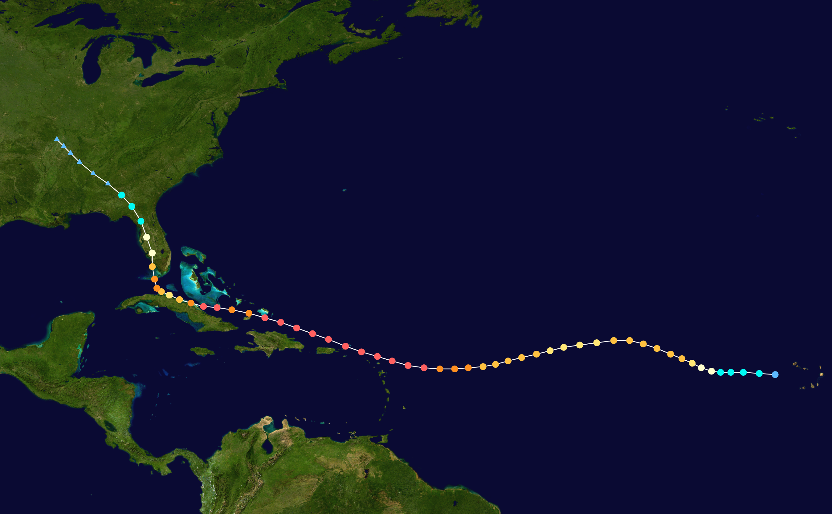
A compelling detailed picture of your temperature regulator hypothesis, Willis. This is ready for a reprise of your EE paper. Perhaps you should also consider a shot at converting this to a model for framing and constraining general circulation models given that you are dealing with control on the energy input into the system. Rather it should replace the parameterization they currently use for clouds and their over hyped aerosol fudge factor which is the “regulator” the Team uses to conserve a high climate sensitivity for CO2. Yeah, on second thought, not much chance of collaboration here.
Willis, how do they get the data for the HadSLP2 gridded dataset of sea level pressure? I only ask in case they calculate it using data that you’re using elsewhere in your calculation and it is thus correlating with itself.
The HadSLP2 dataset comes from a number of stations all around the planet. In addition, it’s a small contributor to the final calculation. Hang on, let me look … ok, the pressure term only makes a difference of about 1% in the final calculation. So however the Hadley folks get it, it’s making little difference.
w.
I had similar questions.
Thinking out loud, I’m trying to figure out what the location of the cloud top physically signifies. Is it the point at which a local parcel of air, rising and cooling at the saturated adiabatic lapse rate, runs out of condensable water to sustain more cloud formation? If so, would one also expect this amount of available condensable water, and thus cloud-top height, to be proportional to the temperature of the air at the ocean surface where convection is initiated, and thus the observed correlation in figure 5 would be expected?
Strictly, I wouldn’t expect it to be linear, but it might appear so over relatively small temperature ranges.
Really good Willis. Here is some stuff posted on wattsup over previous months/years that may help tie it all together.
Best, Allan
https://www.facebook.com/photo.php?fbid=1527601687317388&set=a.1012901982120697.1073741826.100002027142240&type=3&theater
https://www.facebook.com/photo.php?fbid=1665255773551978&set=a.1012901982120697.1073741826.100002027142240&type=3&theater
The correct mechanism is described as follows (approx.):
Equatorial Pacific Sea Surface Temperature up –> Equatorial Atmospheric Water Vapor up 3 months later –> Equatorial Temperature up -> Global Temperature up one month later -> Global Atmospheric dCO2/dt up (contemporaneous with Global Temperature) -> Atmospheric CO2 trends up 9 months later
What drives Equatorial Pacific Sea Surface Temperature? In sub-decadal timeframes, El Nino and La Nina (ENSO); longer term, probably the Integral of Solar Activity.
The base CO2 increase of ~2ppm/year could have many causes, including fossil fuel combustion, deforestation, etc, but it has a minor or insignificant impact on global temperatures.
The Nino34 Area Sea Surface Temperature (the blue line in the above upper plot), adjusted by the Sato Global Mean Optical Depth Index (for major volcanoes – the yellow line), correlates quite well with the Global UAH LT temperature four months later (the red line).
UAH LT temperature also correlates well with Equatorial Atmospheric Water Vapor of one month earlier (the yellow line in the above lower plot). This mechanism ties to Willis’ clouds – down to the hourly level – the rising Sun drives water vapor off the oceans into the atmosphere, clouds form, shade the ocean, and that is the natural regulator of temperature.
This close correlation of Nino34 SST’s with global temperatures four months later either means that this small Nino34 area of the Pacific Ocean drives global temperature or other tropical oceanic areas have a similar temperature signature – that they correlate with Nino34 SST’s.
How does CO2 play into this equation? Atmospheric CO2 is increasing at a “base rate” of about 2ppm/year, probably due to fossil fuel combustion, deforestation, etc. However, the rate of change dCO2/dt changes ~contemporaneously with average global temperature, and its integral, the trend of atm. CO2 changes ~9 months after global temperature, so it is clear that global temperature drives atm. CO2 much more than atm. CO2 drives temperature, and so the sensitivity of temperature to atm. CO2 must be relatively small, and far too small for a real global warming crisis to exist.
It appears to be just about that simple! And the very-scary global warming climate models do not reflect this mechanism at all. I suggest we can do a much better job of modelling climate with the simple closed-form solutions presented in these plots, maybe with a bit more refinement – and they will show NO GLOBAL WARMING CRISIS.
More details here
https://wattsupwiththat.com/2018/05/02/is-climate-alarmist-consensus-about-to-shatter/comment-page-1/#comment-2805310
and here
https://wattsupwiththat.com/2018/04/28/solar-activity-flatlines-weakest-solar-cycle-in-200-years/comment-page-1/#comment-2803244
Correction
“UAH LT temperature also correlates well with Equatorial Atmospheric Water Vapor of one month earlier (the yellowISH-GREEN line in the above lower plot).
Allan,
Please forgive me if I am stating the blindingly obvious. I doing so just to clear up my own thoughts.
you say:
“What drives Equatorial Pacific Sea Surface Temperature? In sub-decadal timeframes, El Nino and La Nina (ENSO); longer term, probably the Integral of Solar Activity.”
If you accept that El Nino and La Nina events (i.e. the ENSO “cycle”) drives the Nino3.4 central-Pacific SST in sub-decadal timeframes then Willis’ results would seem to imply that:
a) the warming of these SST’s invokes a cooling response through the increase of cloud-height and an increase in the area of cumulus clouds.
b) the cooling of these SST’s invokes a warming response through the decrease of cloud-height and a decrease in the area of cumulus clouds.
Hence, Willis has found the underlying regulatory mechanism that is keeping the equatorial atmospheric temperatures within a very limited range i.e. a mechanism that produces a negative feedback upon the equatorial atmospheric temperatures over sub-decadal time frames, and possibly longer.
So I think it would be fair to say that Willis has found the mechanism that mitigates against atmospheric temperature changes from the long-term mean. However, he is not saying that this mechanism is causing those temperature changes in the first place.
Thanks in advance for bearing with my ramblings…..
Hello Ian,
Thank you for your question. I cannot speak for Willis but I can speak to the parts of the mechanism that I addressed. I will try to note what is speculation and what is demonstrated by correlated data.
I wrote above:
“The correct mechanism is described as follows (approx.):
Equatorial Pacific Sea Surface Temperature up –> Equatorial Atmospheric Water Vapor up 3 months later –> Equatorial Temperature up -> Global Temperature up one month later -> Global Atmospheric dCO2/dt up (contemporaneous with Global Temperature) -> Atmospheric CO2 trends up 9 months later.”
– This is all fairly well-proved – one question I have is what primarily drives the close dCO2/dt vs temperature relationship – is it primarily the Henry’s Law solution/exsolution of CO2 from seawater, or does the huge temperature-driven mostly-land-based seasonal photosynthesis/oxidation flux predominate?
Continuing, I wrote:
“What drives Equatorial Pacific Sea Surface Temperature? In sub-decadal timeframes, El Nino and La Nina (ENSO); longer term, probably the Integral of Solar Activity.”
– The ENSO cyclical global temperature driver is well-proven, imo; the bigger question is what drives long term ocean warming and cooling, and I think it must be the integral of solar activity, but I have not proved it. Dan Pangburn and others have made a good effort to do so.
Continuing, I wrote:
“The base CO2 increase of ~2ppm/year could have many causes, including fossil fuel combustion,
deforestation, etc, but it has a minor or insignificant impact on global temperatures.”
– Increasing atmospheric CO2 may play a minor role in global warming, but it is certainly minor and probably almost insignificant.
As I see it (obviously subject to correction by Willis), what Willis has described is a self-regulating system, that effectively provides a negative feedback to the oceanic climate system by increasing cloud cover when the ocean warms due to sunshine, such that this warming is moderated. I speculate that over long periods of time, sea surface temperatures can warm provided solar activity exceeds a certain threshold. The feedback effect will not completely prevent this warming, but will moderate it. I presume the same principles apply in reverse in a long term cooling situation.
Brilliant. Persistance always pays off. Five quarts of medals for Komrad Willis.
Sandy, Minister of Future
Ah…intuition followed by facts and data. So old fashion. So reliable.
And that sir, is why I always read your posts.
This id one of Willis’ most interesting posts. I especially liked the idea of looking at the Earth from the point of view of the Sun which helps simplify the more complex processes. The article has some of the most original and convincing ideas on this mechanism for temperature control by real forces, not CO2. I look forward to Willis developing this idea further,
Looking at the Earth from the point of view of the Sun totally wowed me when I read it here first all those years ago. A brilliant insight.
On today’s post the most peculiar thing is that the correlation is so good. Too good.
It seems that nucleation points for clouds are always in great abundance so there absence doesn’t ever matter. Perhaps the formation of ice crystals is part of the mechanism?
Because otherwise I can’t see how this can be so good.
Hello M,
Your dad Richard S C would love this post – please make sure he sees it (and my above comments), and give him my best regards.
Thank you, Allan
Allan MacRae:
This is a public reply from me to your comment made here to my son. This public reply also includes my reply to your private email to me. .
Firstly, sincere thanks for informing me of this WUWT item which is very good and, as you suspecte,, it does fascinate me (and I am glad to have survived long enough to have read it). Indeed, I suspect that in future Willis Eschenbach will be honoured for this in the same way that Milankovitch (a cement engineer) is honoured by having his climate related cycles named after him.
I also like your post that you point me to. Yes, you do provide very supporting data for the postulated ‘Eschenbach Effect’. And I will add to the structure of supporting information in a post below the comments on the data of rogertaguchi ( at https://wattsupwiththat.com/2018/05/09/clouds-and-el-nino/#comment-2811635 ) and you.
Thankyou for your concern for my health which I reciprocate. I hope and pray that your medical problems will be resolved or at least not be too painful.
My pain relief is morphine-based and inhibits my thought. Therefore, I have to reduce that relief (and obtain significant suffering) to enable me to make posts such as this. Hence, I am grateful for the kind and unduly flattering comments in your email but I hope you will understand my reticence to make frequent comments on WUWT.
Also, I would be more willing to make the effort to provide posts on WUWT if my every post were not savaged by trolls and stalkers some of whom I suspect to be bots (e.g. Mark W), or if I were given some protection. Indeed, I was banned from one thread about me because I requested to know of what I was being accused ( see https://wattsupwiththat.com/2014/05/12/a-mann-uva-email-not-discussed-here-before-claims-by-mann-spliced-and-diced/.).
Richard
richardscourtney May 9, 2018 at 11:43 pm
Richard, thank you profoundly for your most kind words above, undeserved though they may be. I’m sorry to hear about your troubles. Constant unremitting pain is a great weight to bear, so I’m glad to see that you are maintaining your spirit through it all.
I am sure I speak for many here when I wish you the very best, along with the hope that your pain goes into remittance.
My warmest regards to you,
w.
Is your typo “id” for “is” a Freudian slip? 🙂
“thunderstorms cool the surface in part by increasing surface albedo. And while the change is small, about half a percent, it represents a change of ~ 4 W/m2 in absorbed solar energy. This is more change in absorbed energy than would result from a doubling of CO2.”
Yes but the 3.7 W/m^2 of CO2 is average for the global surface area and lasts over 100 years. That 4 W/m^2 covers the area under thunderstorms and lasts an hour or so. Anyway I agree with the cloud negative feedback and that means TCR should be less than 1 C per 2x CO2
Hi, Dr. Strangelove! I agree with your judgment on cloud negative feedback and TCR. But the 3.7 W/m^2 value for radiative forcing is not averaged for the global surface area for a clouded Earth. It comes from computer calculations of CO2 absorption changes on doubling concentration, necessarily for a CLOUDLESS surface [see Gunnar Myhre et al. “New estimates of radiative forcing due to well mixed greenhouse gases” at Geophysical Research Letter, Vol. 25, No. 14, PP 2715-2718, July 15, 1998]. Their Table 3 shows their derivation of “delta F” = 5.35 ln(C/Co) for radiative forcing, and substituting C/Co = 2 gives 5.35 ln2 = 3.7 W/m^2. This can be used to calculate climate sensitivity of 1 degree on doubling CO2, not counting feedbacks (which the IPCC wrongly says triples the value to 3 degrees).
Why do clouds decrease climate sensitivity? There are 3 factors involved. First, cloud particles (small liquid droplets or ice crystals) are almost perfect black bodies (emissivity 0.98 or greater) at infrared (IR) frequencies, so the cloud-tops act as the source of the initial IR radiation to be absorbed by CO2 molecules in the path length to outer space. At temperatures well below 288 K (15 Celsius), the initial radiative flux at all IR frequencies are lower than at the Earth’s surface (the Planck radiation law, and integrated, the Stefan-Boltzmann law). Doubling CO2 cannot increase absorption above 100%, so has little effect below the cloud tops.
Secondly, the path length of absorbing CO2 molecules is shorter from the cloud tops to outer space, compared to from the Earth’s surface to outer space. As air pressure/concentration of CO2 decreases exponentially with increasing altitude, the number of ground state CO2 molecules in the path length decreases more-than-linearly.
Thirdly, the central IR frequencies (around 667 cm^-1) are almost completely saturated. Doubling CO2 will increase absorption only for frequencies in the wings of the absorption ditch. The MODTRAN computed spectra available at https://en.wikipedia.org/wiki/Radiative_forcing show only a tiny difference (between the blue and green curves), centered at 618 and 721 cm^-1. These absorptions involve photons absorbed by molecules in the bond-bending first excited state, 667.4 cm^-1 above the ground vibrational state [see http://www.barrettbellamyclimate.com , “Spectral transitions”, Diagram 3]. The equilibrium ratio of the number of first excited state to ground state molecules varies as the decreasing exponential Boltzmann function exp(-hcf/kT) where f = 667.4 cm^-1 is the wavenumber and c = 2.998 x 10^10 cm/s is the vacuum speed of light, and k is Boltzmann’s constant. T is the absolute temperature, and since it is in the denominator, the ratio of first excited states plummets as temperatures decrease with increasing altitude.
The bottom line is that when the 62% of the Earth’s surface covered by clouds is considered, doubling CO2 decreases climate sensitivity (not including feedbacks) from 0.9 K to 0.6 K (the value of 0.9 K results from using radiative forcing = 3.39 W/m^2 , as shown in the MODTRAN spectrum, instead of 3.7 W/m^2). And this result was derived using average cloud tops at 278.85 K (5.7 Celsius) at an altitude of 1.37 km. Willis’ graphs show cloud tops, especially at the tropics, at much higher altitudes, so the decrease in climate sensitivity (not counting feedbacks) could be significantly greater.
And this doesn’t include narrowing of vibration-rotation line widths with lower temperatures (smaller Doppler shifts) and lower pressures (less pressure broadening) at higher altitudes, which will decrease the contribution to total absorption from above the cloud tops even more.
The MODTRAN spectrum was calculated for upward irradiance at 20 km, and showed no difference in the CO2 truncation levels (at “220 K” for both 300 and 600 ppmv CO2). However, if the integration is done to 70 km, the increasing temperatures in the stratosphere above 20 km mean that doubling CO2 will increase EMISSION at central frequencies around 667 cm^-1 [see the section “The hard bit” at http://www.barrettbellamyclimate.com ]. Therefore for energy balance, the Earth’s surface does not need to warm up as much; I.e. climate sensitivity is decreased even further.
The bottom line is that climate sensitivity (not including feedbacks) is slightly below 0.6 K. Even including a 50% positive feedback from increasing water vapor, in agreement with Soden & Held’s “An Assessment of Climate Feedbacks in Coupled Ocean-Atmosphere Models”, Journal of Climate, Vol. 19, pp. 3354-3360 (2006), would boost climate sensitivity to only 0.9 K. Therefore wrecking Western economies in order to decrease warming to only 2 K is unnecessary, wasteful and foolish.
And as Willis has shown, increasing temperatures which increase water vapor which increases clouds result in a negative feedback, in agreement with physical intuition. Therefore climate sensitivity can be dropped down from 0.9 K to 0.6-0.7 K . Email me at rtaguchi@rogers.com if you want more details of this calculation.
BTW, the rise and fall of El Nino temperature spikes and the recovery from the Mt. Pinatubo eruption show that there is no decades- or centuries-long time constant (if there were such a long lag period, then temperatures should have continued to increase even if CO2 had been constant in the last 20 years instead of continually increasing).
+1 (for each paragraph)
rogertaguchi: good post. thank you.
Roger T wrote:
“And as Willis has shown, increasing temperatures which increase water vapor which increases clouds result in a negative feedback, in agreement with physical intuition. Therefore climate sensitivity can be dropped down from 0.9 K to 0.6-0.7 K .”
Thank you Roger for you post. I agree with you that Climate Sensitivity (CS) to increasing atm. CO2 is impacted by negative feedbacks, and is less than ~1.0C/(2xCO2).
I further suggest that CS is MUCH less than 1.0C, and is probably closer to 0.0C than 1.0C – in any case, far too low to cause any real global warming crisis.
My evidence is derived from world-scale data as evidence such as my two posts above from earlier today, which tie well with Willis’ world-scale observations. Your observations on the rapid (few-years) rebound from Pinatubo are also supported by world-scale data.
Comments welcomed. I will send you my email should you prefer to talk offline.
Best, Allan
The ChicagoU web version of MODTRAN is not capable of simulating the conditions measured above certain tropical ocean at SST of 28C. The OLR above the Coral Sea often averages below 200W/sq.m.
https://neo.sci.gsfc.nasa.gov/view.php?datasetId=CERES_LWFLUX_M
Taking the MODTRAN water scale to its maximum and with 75mm/hr of rain the lowest value of OLR it produces is 209w/sq.m. CERES shows monthly averages on a 1 degree grid of 195W/sq.m.
Putting water vapour to the highest possible value available in the model reduces CO2 sensitivity to 1W/sq.m.
rogertaguchi and Allan MacRae :
Allan says to rogertaguchi ,
“Thank you Roger for you post. I agree with you that Climate Sensitivity (CS) to increasing atm. CO2 is impacted by negative feedbacks, and is less than ~1.0C/(2xCO2).
I further suggest that CS is MUCH less than 1.0C, and is probably closer to 0.0C than 1.0C – in any case, far too low to cause any real global warming crisis.”
YES!
Empirical – n.b. not model-derived – determinations indicate climate sensitivity is less than 1.0 deg.C for a doubling of atmospheric CO2 equivalent. This is indicated by the studies of
Idso from surface measurements
http://www.warwickhughes.com/papers/Idso_CR_1998.pdf
and Lindzen & Choi from ERBE satelite data
http://www.drroyspencer.com/Lindzen-and-Choi-GRL-2009.pdf
and Gregory from balloon radiosonde data
http://www.friendsofscience.org/assets/documents/OLR&NGF_June2011.pdf
These determinations use different methods to analyse different data sets and they each deterrmine that climate sensitivity is 0.4 deg C for a doubling of CO2 equivalent.
Richard
Roger
Yes 3.7 W/m^2 is for clear sky. Increase emission in stratosphere leads to expected “stratospheric cooling” due to GHE. The cooling will not reach the surface as the troposphere has different temperature profile.
See discussion on CO2 saturation
https://scienceofdoom.com/2010/05/12/co2-an-insignificant-trace-gas-part-eight-saturation/
Yes TCR probably low. Lindzen estimated 0.6 or 0.7 K. Thanks for info
To Dr. Strangelove re comment of May 10 at 5:31 am: Thank you for your courteous reply. You have obviously taken the time to research my point, and have courageously posted that the 3.7 W/m^2 is for a clear sky, as I stated. I have used Wikipedia numbers in my calculation to show that even using their assumptions the IPCC best value of 3 K for equilibrium climate sensitivity (ECS) is way too high. I note that the Wikipedia articles on climate skeptics Richard Lindzen of MIT and William Happer of Princeton include personal attacks. For instance, Lindzen has admitted being wrong in a paper, something that every fair-minded scientist ought to do (and every researcher on the frontier makes mistakes), but this seems to be held against him. Admitting mistakes is something that the CAGW (Catastrophic Anthropogenic Global Warming) cult seems unable to do. Happer has made cutting edge discoveries and innovations, but has been dismissed as being against the 97% consensus; i.e. he is a weirdo that can be safely and justifiably ignored.
Re your point that “cooling will not reach the surface as the troposphere has a different temperature profile” [from the stratosphere]: Doubling CO2 will raise the altitude at which central frequencies (around 667 cm^-1) finally escape to outer space, and due to the temperature inversion from 20 km to 50 km caused by absorption of incoming UV and visible radiation by ozone, this emission will be at a higher “temperature”. This increased emission at 667 cm^-1 means that the Earth’s surface does not have be warmed AS MUCH to achieve total energy balance when all frequencies are emitted at 288 K. I.e. ECS is decreased. This does not mean that energy has to be transferred from the stratosphere to the troposphere to the surface; radiative exchange might change the temperature at the tropopause slightly, but does not have to extend all the way to the surface. Convection cannot transfer net heat from the stratosphere to the surface, since “heat rises” by convection.
IMO the literature argument re altitude of final emission to outer space is wrong when extended to frequencies in the wings of the CO2 absorption band which are not 100% saturated. For example: “doubling CO2 means the final escape of IR photons occurs at higher altitudes where the temperature of the troposphere is lower; this decreased emission means that for total energy balance the surface temperature of the Earth must go up”. This argument uses the Schwarzschild Equation I = Io.exp(-KCL) + B[1-exp(-KCL)] , assuming that the first term (Beer-Lambert transmission) is zero, so the radiative flux I = B , where B is the Planck black body emission whose integrated value over all frequencies gives the Stefan-Boltzmann T^4 law. This is adequate for central CO2 frequencies around 667 cm^-1 which escape in the stratosphere from 20 to 50 km, as I have already said.
But for frequencies in the wings that are not completely saturated, let the Signal observed by satellites looking downward onto the Earth’s surface be I/Io = exp(-KCL) + (B/Io)[1-exp(-KCL)]. Since exp(-KCL) is the transmittance = 1-A, where A is the absorbance (consistent with Kirchhoff’s Law that a good absorber is a good emitter), the Signal becomes I/Io = 1-A + (B/Io)A = 1 – (1-B/Io)A , which is simply a modified Beer-Lambert absorption where -B/Io takes into account the emission at final altitude where the temperature is lower than the 288 K at the Earth’s surface. I.e. the CO2 spectrum in the wings is an ABSORPTION spectrum, not an EMISSION spectrum. The literature is laughably wrong on this point, as any competent chemist can tell you. Because CO2 667 cm^-1 emission occurs near the peak of black body emission at Earth temperatures, B/Io at 10 km can be approximated by (220/288)^4 = 0.34, so the Signal becomes I/Io = 1 – 0.66A, where A is unmodified Beer-Lambert absorbance. Because the temperature from 10 to 20 km is roughly constant at 220 K (due to absorption of incoming solar radiation by ozone), the Signal at 10 km will be unchanged all the way to 20 km (because there can be no net heat flow by absorption & emission from one region to another at the same temperature – the 2nd Law of Thermodynamics), even as the concentration of absorbing molecules decreases by a factor of 6 or so. So effectively final escape of photons at unsaturated frequencies occurs at 10 km (and not at intermediate altitudes such as 4 or 5 km), with a Signal = 1 – 0.66A. So as CO2 is doubled, A increases slightly (with saturation effects becoming important for A greater than 0.1 or 0.2), the Signal escaping to outer space decreases slightly, requiring a slight increase in the Earth’s surface temperature in order to increase Io for energy balance. The energy source for this increase in temperature is the constant incoming Solar radiation (if outflow is slightly throttled back, a constant inflow will increase the surface temperature which radiates more as T^4 until a new steady state is quickly achieved).
I trust this discussion helps Dr. Strangelove, who sincerely wants to understand more, as well as others with open minds. With respect for all.
The 4W/m^2 is for surface albedo, a tiny component of the system. The power of a moderate thunderstorm at 1″ per hour is 15,924 W/m^2. That is why the process is so stable. The capacity of water to transport and reject heat is 3 or more orders of magnitude greater than the miniscule effect of CO2. Willis is right, small timescale processes with nearly unlimited headroom make for a brick wall of control.
So … How does this regulator allow either a slow drift to glacial cold of 8 degrees C or a rapid decline to little ice age of 12 degrees C?
Sandy, Minister of Future
Odd!?
Willis demonstrates an Earth heat regulating that caps daily temperature increases.
Then you, Sandy, demand futuristic Earth cooling explanations for unnamed mechanisms…
Twisted, bizarre and out of touch with reality logic.
@ATheoK- you need a refresher course in trolling 101 hahaha.
You said:
1. Then you, Sandy, demand futuristic Earth cooling explanations for unnamed mechanisms…
* my question was hardly a demand.
‘slow drift to glacial cold’ and ‘rapid decline’ are in no way futuristic.
And …
2. Twisted, bizarre and out of touch with reality logic.
* if it’s logical it can hardly be twisted, bizarre, or out of touch with reality. Get a grip.
Sandy, Minister of Future
Typical trollop response:
A) Respond with an ad hominem to demean the commenter.
B) Introduce straw men arguments to skew the logic.
C) Twist words and meanings as a false buttress for the trollop.
Blunt question? It’s a demand.
“‘slow drift to glacial cold’ and ‘rapid decline’ are in no way futuristic.”
It is future, until you define the time period.
“* if it’s logical it can hardly be twisted, bizarre, or out of touch with reality. Get a grip.
A bogus straw man where Sandy substitutes a different word for the word I used. Logic is not equal to logical!
All in all, a completely bogus argument from Sandy.
“The slow drift to glacial cold” depends on the insolation at high latitudes which can hardly be governed by tropical thunderstorms.
An as for “a rapid decline to little ice age of 12 degrees C” there hasn’t been any. The decline from MWP to LIA was on the order of 1 degree grobally. Just what are you thinking of?
It is precisely for studies such as these that we included clouds with the radiation measurements. Keep up the good work.
Pnmn, are you associated with the CERES project?
w.
From the sun you can see the entire surface of the planet over 24 hrs appear as it rotates before your eyes.
From a single geostationary satellite you can only see the same part of the planet all the time, and less surface area than you can see from the sun, even when the entire surface is illuminated at geostationary midday. You can’t see the poles from geostationary orbit, no matter what season it is.
One question that jumps out at me is does this work worldwide. Instead of just the Nino 3.4 region, how have cloud temperatures changed over the entire planet over time? Is it consistent across latitudes? How does it correlate to temperature change?
If clouds work as a negative feedback then we should see a correlation. Colder clouds mean higher clouds which means more water vapor has been extracted. This would reduce the GHE due to water vapor.
Not the GHE but the feedback to the GHE
Thunderstorms occur worldwide, generally during warm seasons.
“Colder clouds mean higher clouds which means more water vapor has been extracted”
Higher cloud tops mean taller and often larger clouds.
Increased cloud area generally means greater volumes of moisture are present; not reduced.
Your question regarding GHE is misstated. Unlike CO₂ water, H₂O, is IR active during all three physical states; solid, liquid, vapor.
Meaning, clouds intercept/emit large portions of the infra-red spectrum, no matter which H₂O physical state those wavelengths encounter.
Cold cloud tops that are mostly ice crystals with very high albedo that reflects substantial portions of the entire light spectrum.
Water, H₂O, is the atmospheric GHE whale, while CO₂ is a GHE atmospheric flea.
ATheoK : “Increased cloud area generally means greater volumes of moisture are present; not reduced.”
Not necessarily where it counts. Warmer/moist air would lead to enhanced convection driving water vapor higher into the atmosphere where it is colder. This condenses out more water vapor into water/ice (aka clouds). IOW, while you may start with a little more moisture you have a more efficient condensation process removing even more.
Keep in mind that the clouds then deposit some the water that was condensed out back to the surface in the form of rain/snow. This leaves dryer air aloft where the GHE is most important. We should see an overall slight increase in precipitation as well.
I looked up the emissivity coefficient for water. Pretty darn close to the same values.
Water 0.95 – 0.99
Ice (rough) 0.985 (smooth) 0.966
snow 0.969 – 0.997
Now the tropical oceans are just about the only areas on Earth with a heat surplus. Even the Sahara desert has a net heat deficit. The heat exported from the tropical oceans (and particularly the Pacific Warm Pool) therefore strongly affects the climate of the whole planet.
now that is some science sir … well done
The other parameter in T-Storm development is the temperature lapse rate of the atmosphere. To get the warm, moist air to continue rising, it basically needs to stay warmer than the surrounding air it is rising into. This air cools as it rises, so if the air above it is too warm as in a temperature inversion, the air stops rising and everything is capped.
In coastal North Carolina in the summer for instance, at noon the air temperature may be 92F with dew points in the 70’s. But the best we can get are cumulus clouds because the upper air temperatures are too warm to generate T-Storms. Yet you can be at the beach and look out at towering T-Storms over the Gulf Stream because the air masses are different enough to allow it.
It would be a different story if the maritime air in the tropics was more continental in nature.
Central Pacific OLR (inverted cloud proxy), MEI, HadSST3, and equatorial OHC 1979-2017: ?dl=0
?dl=0 ?dl=0
?dl=0
El Ninos drive clouds. OHC drives El Ninos. TSI-insolation drives OHC.
Amazing correlations, it would be difficult to find a more compelling evidence on anything.
Great post Willis. Congratulations.
Sorry to beat a dead horse, but can you not see the solar cycle when looking at fig. 4? Especially if you remove the el nino spikes in 2010 and 2016?
Nope.
w.
Yes …. it does look that way doesn’t it. When you consider the later post by coolclimate, … makes sense. But, I would speculate.ate that this effect is restricted to just the tropical zones. As Willis noted, even his cloud study doesn’t hold up well in the higher lats.
The affect of clouds varies by latitude, and darkness. Check this out from 2001:
https://www.giss.nasa.gov/research/briefs/tselioudis_01/
RH May 9, 2018 at 7:03 am
So your plan is to remove the El Nino signal from the NINO3.4 area???
… Just how would you plan to do that, and what do you think would remain?
Which is why I said “Nope” above …
w.
Not remove the NINO3.4 signal entirely, but run it through a low pass filter to take out the major 1 to 2 year events. What would be left, I believe, would be well correlated with solar cycles. Unfortunately, I lack your giant brain or skills with data vis.
Thanks, RH, but no:
Different start, different end, different inflection points … not seeing it.
w.
Hmm, freq looks about right but with a two year delay. No Mas! thanks for humoring me.
rh May 9, 2018 at 3:50 pm
Seriously? What about the start and the end? And you are calculating the frequency from a sorta-kinda association that lasts half a cycle?
w.
Willis, I must give you the credit for leading me down this path of thinking. In the desert environment, as well as the other very low humidity environments, the daily temperature change can be extreme. What this tells us is that despite the extreme daytime high temperature, the amount of heat stored in the atmosphere is rather minuscule.
Is there a mechanism to calculate the Joules of energy (heat) transported by the thunderstorms rather than simply measuring the average kinetic energy of the particles (temperature) in the atmosphere or ocean?
The “eyeball” and SWAG would tell us that the far greater TS heights in the PWP zone are transporting tremendous amounts of heat to space.
I recognize it would require humidity data to overlay with the temperature.
Convective available potential energy – CAPE
http://tornado.sfsu.edu/geosciences/classes/m201/buoyancy/CAPE_Procedure.html
Most of the energy is actually being transferred to higher latitudes where the air descends and creates high pressure cells where it then radiates energy into space — the horse latitudes. Much of the region of the horse latitudes actually radiate more energy into space than they receive directly from the sun.
This is one reason I seriously question models based solely upon temperature input. Trying to come up with a global temperature that describes global warming (heat) means you are making the assumption that humidity doesn’t matter and/or is the same everywhere on the globe.
Even IPCC admits that more heat is removed from the surface by convection than by IR radiation. But they don’t exactly dwell on it since climate models can’t handle convection realistically.
The vertical convection of heat is what keeps my doubts high about climate models. The models deal with temperature, not heat content. Convective heat transfer will occur at all latitudes not just the tropics. Otherwise, how does precipitation occur?
PRDJ May 9, 2018 at 12:55 pm
Thanks, PRDJ. Much as I distrust the model, your objection simply isn’t true. The models absolutely do deal with heat content. Scientists may be wrong but they are rarely imbeciles …
w.
OK, fair enough. Thanks Willis.
Good post. I can see why the GCMs do not directly simulate clouds, as the effect looks large enough to overwhelm any effect from CO2.
The same clouds which have a cooling affect during the day will have a warming affect during the night. Any idea what the difference is, and whether it’s a net cooling or warming?
If I remember correctly, the tropical pattern has ferocious afternoon thunderstorms followed by clear skies by 9PM almost every night. These clouds don’t stick around to prevent heat loss to space at night.