Guest essay By Christopher Monckton of Brenchley
This series discusses climatology’s recently-discovered grave error in having failed to take due account of the large feedback response to emission temperature. Correct the error and global warming will be small, slow, harmless and net-beneficial. The series continues to attract widespread attention, not only here but elsewhere. The ripples are spreading.
My reply to Roy Spencer’s piece on our discovery at drroyspencer.com has attracted 1400 hits, and the three previous pieces here have attracted 1000+, 350+ and 750+ respectively. Elsewhere, a notoriously irascible skeptical blogger, asked by one of his followers whether he would lead a thread on our result, replied that he did not deign to discuss anything so simple. Simple it is. How could it have been thought the feedback processes in the climate would not respond to the large pre-existing emission temperature to the same degree as they respond to the small enhancement of that temperature caused by adding the non-condensing greenhouse gases to the atmosphere? That is a simple point. But simple does not necessarily mean wrong.
The present article develops the math, which, though not particularly complex, is neither simple nor intuitive. As with previous articles, we shall answer some of the questions raised in comments on the earlier articles. As before, we shall accept ad interim, ad argumentum or ad experimentum all of official climatology except what we can prove to be incorrect.
Let us conduct a simple Gedankenexperiment, running in reverse the model of Lacis et al. (2010), who found that, 50 years after removing all the non-condensing greenhouse gases from the atmosphere, the climate would have settled down to a new equilibrium, giving a slushball or waterbelt Earth with albedo 0.418, implying emission temperature 243.3 K. We shall thus assume ad experimentum that in 1800 there were no greenhouse gases in the atmosphere. For those unfamiliar with the logical modes of argument in scientific discourse, it is not being suggested that there really were no greenhouse gases in 1800.
Lacis found that, only 20 years after removal of the non-condensing greenhouse gases, global mean surface temperature would fall to 253 K. Over the next 30 years it would fall by only 1 K more, to 252 K, or 8.7 K above the emission temperature. Thus, subject to the possibility that the equatorial zone might eventually freeze over, surface temperature in Lacis’ model settled to its new equilibrium after just 50 years.
One question which few opponents in these threads have answered, and none has answered convincingly, is this: What was the source of that additional 8.7 K temperature, given that there were no non-condensing greenhouse gases to drive it? Our answer is that Lacis was implicitly acknowledging the existence of a feedback response to the 243.3 K emission temperature itself – albeit at a value far too small to be realistic. Far too small because, as shown in the previous article, Lacis allocated the 45.1 K difference between the implicit emission temperature of 243.3 K at the specified albedo of 0.418 and today’s global mean surface temperature of 288.4 K (ISCCP, 2018) as follows: Feedback response to emission temperature 252 – 243.3 = 8.7 K; warming directly forced by the naturally-occurring, non-condensing greenhouse gases (288.4 – 252) / 4 = 9.1 K, and, using Lacis’ feedback fraction 0.75, feedback response to warming from the non-condensing greenhouse gases 27.3 K: total 45.1 K. This asymmetric apportionment of the difference between emission temperature and current temperature implies that the 8.7 K feedback response to emission temperature is only 3.6% of 243.3 K, while the 27.3 K feedback response to greenhouse warming is 300% of 9.1 K. Later we shall demonstrate formally that this implausible apportionment is erroneous.
It will be useful to draw a distinction between the pre-industrial position in 1850 (the first year of the HadCRUT series, the earliest global temperature dataset) and the industrial era. We shall assume all global warming before 1850 was natural. That year, surface temperature was about 0.8 K less than today (HadCRUT4) at 287.6 K, or 44.3 K above emission temperature. Lacis’ apportionment of the 44.3 K would thus be 8.7 K, 8.9 K and 26.7 K.
We shall assume that Lacis was right that the directly-forced warming from adding the naturally-occurring, non-condensing greenhouse gases to the air was 8.9 K. Running the experiment in reverse from 1850 allows us to determine the feedback fraction implicit in Lacis’ model after correction to allow for a proper feedback response to emission temperature. Before we do that, let us recall IPCC’s current official list of feedbacks relevant to the derivation of both transient and equilibrium sensitivities:

IPCC’s chosen high-end feedback sum implies Charney sensitivities somewhere between minus infinity and infinity per CO2 doubling. Not a particularly well constrained result after 30 years and hundreds of billions of taxpayers’ dollars. IPCC’s mid-range feedback sum implies a mid-range Charney sensitivity of only 2.2 K, and not the 3.0-3.5 K suggested in previous IPCC reports, nor the 3.3 K in the CMIP3 and CMIP5 ensembles of general-circulation models. No surprise, then, that in 2013, for the first time, IPCC provided no mid-range estimate of Charney sensitivity.
None of the feedbacks listed by IPCC depends for its existence on the presence of any non-condensing greenhouse gas. Therefore, in our world of 1800 without any such gases, all of these feedback processes would be present. To induce a feedback response given the presence of any feedback process, all that is needed is a temperature: i.e., emission temperature. Since feedback processes are present, a feedback response is inevitable.
Emission temperature is dependent on just three quantities: insolation, albedo, and emissivity. Little error arises if emissivity is, as usual, taken as unity. Then, at today’s insolation of 1364.625 Watts per square meter and Lacis’ albedo of 0.418, emission temperature is [1364.625(1 – 0.418) / d / (5.6704 x 10⁻⁸)]0.25 = 243.3 K, in accordance with the fundamental equation of radiative transfer, where d, the ratio of the area of the Earth’s spherical surface to that of its great circle, is 4. Likewise, at today’s albedo 0.293, emission temperature would be 255.4 K, the value widely cited in the literature on climate sensitivity.
The reason why official climatology has not hitherto given due weight (or, really, any weight) to the feedback response to emission temperature is that it uses a degenerate form of the zero-dimensional-model equation, ΔTeq = ΔTref / (1 – f ), where equilibrium sensitivity ΔTeq after allowing for feedback is equal to the ratio of reference sensitivity ΔTref to (1 minus the feedback fraction f). The feedback-loop diagram for this equation (below) makes no provision for emission temperature and none, therefore, for any feedback response thereto.

The feedback loop in official climatology’s form of the zero-dimensional-model equation ΔTeq = ΔTref / (1 – f )
Now, this degenerate form of the zero-dimensional-model equation is adequate, if not quite ideal, for deriving equilibrium sensitivities, provided that due allowance has first been made for the feedback response to emission temperature. Yet several commenters find it outrageous that official climatology uses so simple an equation to diagnose the equilibrium sensitivities that the complex general-circulation models might be expected to predict. A few have tried to deny it is used at all. However, Hansen (1984), Schlesinger (1985), IPCC (2007, p. 631 fn.), Roe (2009), Bates (2016) are just a few of the authorities who cite it.
Let us prove by calibration that official climatology’s form of this diagnostic equation, when informed with official inputs, yields the official interval of Charney sensitivities. IPCC (2013, Fig. 9.43) cites Vial et al. (2013) as having diagnosed the CO2 forcing ![]() , the Planck parameter
, the Planck parameter ![]() and the feedback sum
and the feedback sum ![]() from simulated abrupt 4-fold increases in CO2 concentration in 11 CMIP5 models via the linear-regression method in Gregory (2004). Vial gives the 11 models’ mid-range estimate
from simulated abrupt 4-fold increases in CO2 concentration in 11 CMIP5 models via the linear-regression method in Gregory (2004). Vial gives the 11 models’ mid-range estimate ![]() of the feedback sum as
of the feedback sum as ![]() W m–2 K–1, implying
W m–2 K–1, implying ![]() , and the
, and the ![]() bounds of
bounds of ![]() as
as ![]() , i.e.
, i.e. ![]() .
.
The implicit CO2 forcing ![]() , in which fast feedbacks were included, was
, in which fast feedbacks were included, was ![]() W m–2 compared with the
W m–2 compared with the ![]() W m–2 in Andrews (2012). Reference sensitivity
W m–2 in Andrews (2012). Reference sensitivity ![]() , taken by Vial as
, taken by Vial as ![]() , was
, was ![]() above the CMIP5 models’ mid-range estimate
above the CMIP5 models’ mid-range estimate ![]() . Using these values, official climatology’s version of the zero-dimensional-model equation proves well calibrated, yielding Charney sensitivity
. Using these values, official climatology’s version of the zero-dimensional-model equation proves well calibrated, yielding Charney sensitivity ![]() on
on ![]() , near-exactly coextensive with several published official intervals from the CMIP3 and CMIP5 climate models (Table 2).
, near-exactly coextensive with several published official intervals from the CMIP3 and CMIP5 climate models (Table 2).

From this successful calibration it follows that, though the equation assumes feedbacks are linear but some feedbacks are nonlinear, it still correctly apportions equilibrium sensitivities between forced warming and feedback response and, in particular, reproduces the interval of Charney sensitivities projected by the CMIP5 models, which do account for nonlinearities. Calibration does not confirm that the models’ value ![]() for the feedback fraction or their interval of Charney sensitivities is correct. It does confirm, however, that, at the official values of f, the equation correctly reproduces the official, published Charney-sensitivity predictions from the complex general-circulation models, even though no allowance whatsoever was made for the large feedback response to emission temperature.
for the feedback fraction or their interval of Charney sensitivities is correct. It does confirm, however, that, at the official values of f, the equation correctly reproduces the official, published Charney-sensitivity predictions from the complex general-circulation models, even though no allowance whatsoever was made for the large feedback response to emission temperature.
Official climatology trains its models by adjusting them until they reproduce past climate. Therefore, the models have been trained to account for the 33 K difference between emission temperature of 255.4 K and today’s surface temperature of 288.4 K. They have assumed that one-quarter to one-third of the 33 K was directly-forced warming from the presence of the naturally-occurring, non-condensing greenhouse gases and the remaining two-thirds to three-quarters was feedback response to that direct warming. Therefore, they have assumed that the feedback fraction was two-thirds to three-quarters of equilibrium sensitivity: i.e., that f was somewhere between 0.67 and 0.75.
As a first step towards making due allowance for the feedback response to emission temperature, official climatology’s version of the zero-dimensional-model equation can be revised to replace the delta input and output signals, indicating mere changes in temperature, with entire or absolute values. Note that the correct form of any equation describing natural occurrences (or any natural law) must be absolute values: the use of deltas is only permissible if the delta-equations are correctly derived from the absolute equation. Accordingly, ΔTeq = ΔTref / (1 – f ) should be Teq = Tref / (1 – f ). The revised feedback loop diagram is below:

After amendment to replace delta inputs and outputs with absolute values, official climatology’s form of the zero-dimensional model equation becomes
Teq = Tref / (1 – f )
To find f where the reference and equilibrium temperatures are known, this revised equation can be rearranged as f = 1 – Tref / Teq. In the reverse Lacis experiment, reference temperature Tref before feedback is the sum of emission temperature TE and the additional temperature ΔTE = 8.9 K that is the direct warming from adding the naturally-occurring, non-condensing greenhouse gases to the air. Thus, Tref = TE + ΔTE = 243.3 + 8.9 = 252.2 K. Equilibrium temperature Teq = 287.6 K is simply the temperature that obtained in 1850, after 50 years of the reverse Lacis experiment. Then f = 1 – Tref / Teq = 1 – 252.2 / 287.6 = 0.123, only a fifth to a sixth of official climatology’s value. The reason for the difference is that, unlike official climatology, we are taking correct account of the feedback response to emission temperature.
Next, how much of the 35.4 K difference between Tref = 252.2 K and Teq = 287.6 K is the feedback response to emission temperature TE = 243.3 K, and how much is the feedback response to the direct greenhouse-gas warming ΔTE = 8.9 K? Simply take the product of each value and f / (1 – f) = 0.14, thus: 243.3 x 0.14 = 34.1 K, and 8.9 x 0.14 = 1.3 K. We prove that this is the correct apportionment by using the standard, mainstream form of the zero-dimensional-model equation that is universal in all dynamical systems except climate. The mainstream equation, unlike the degenerate climate-science form, explicitly separates the input signal (in the climate, the 255.4 K emission temperature) from any amplification (such as the 8.9 K warming from adding the non-condensing greenhouse gases to the atmosphere).
The mainstream zero-dimensional model equation is Teq = Tref μ / (1 – μβ), where Tref is the input signal (here, emission temperature); μ = 1 + ΔTref / Tref is the gain factor representing any amplification of Tref such as that caused by the presence of the naturally-occurring, non-condensing greenhouse gases; β is the feedback fraction; μβ is the feedback factor, equivalent to f in climatology’s current version of the equation; and Teq is equilibrium temperature at re-equilibration of the climate after all feedbacks of sub-decadal duration have acted.
The feedback loop for this corrected form of the zero-dimensional-model equation is below:

The feedback loop diagram for the standard zero-dimensional-model equation
Teq = Tref μ / (1 – μβ)
One advantage of using this mainstream-science form of the zero-dimensional model is that it explicitly and separately accounts for the input signal Tref and for any amplification of it via the gain factor μ in the amplifier, so that it is no longer possible either to ignore or to undervalue either Tref or the feedback response to it that must arise as long as the feedback fraction β is nonzero.
It is proven below that the apportionment of the 35.4 K difference between Tref = 252.2 K and Teq = 287.6 K in 1850 derived earlier in our Gedankenexperiment is in fact the correct apportionment. Starting with the mainstream equation, in due time we introduce the direct or open-loop gain factor μ = 1 + ΔTref / Tref. The feedback factor μβ, the product of the direct or open-loop gain factor μ and the feedback fraction β, has precisely the form that we used in deriving the feedback fraction f as 1 – (243.3 + 8.9) / 287.6 = 0.123, confirming that our apportionment was correct.

Note in passing that in official climatology f is at once the feedback fraction and the feedback factor, since official climatology implicitly (if paradoxically) assumes that the direct or open-loop gain factor μ = 1. In practice, this particular assumption leads official climatology into little error, for the amplification of emission temperature driven by the presence of the non-condensing greenhouse gases is a small fraction of that temperature.
But was it reasonable for us to assume that the 287.6 K temperature in 1850, before Man had exercised any noticeable influence on it, was an equilibrium temperature? Well, yes. We know that in the 168 years since 1850 the world has warmed by only 0.8 K or so, and official climatology attributes all of that warming to Man, not Nature.
Was it reasonable for us to start with Lacis’ implicit emission temperature of 243.3 K, reflecting their specified albedo 0.418 on a waterbelt Earth in the absence of the non-condensing greenhouse gases? Why not start with Pierrehumbert (2011), who said that a snowball Earth would have an albedo 0.6, implying an emission temperature 221.5 K? Let’s do the math. The feedback fraction f = μβ would then be 1 – (221.5 + 8.9) / 287.6 = 0.20.
Thus, from a snowball Earth to 1850, the mean feedback fraction is 0.20; from a waterbelt Earth to 1850, it is 0.12; and at today’s albedo 0.293, implying an emission temperature 255.4 K, it is 1 – (255.4 + 8.9) / 287.6 = 0.08. Which is where we came in at the beginning of this series. For you will notice that, as the great ice sheets melt, the dominance of the surface albedo feedback inexorably diminishes, whereupon the feedback fraction falls over time.
Though the surface albedo feedback may have dominated till now, what about the biggest of all the feedbacks today, the water-vapor feedback? The Clausius-Clapeyron relation implies that the space occupied by the atmosphere may (though not must) carry near-exponentially more water vapor – a greenhouse gas – as it warms. Wentz (2007) found that total column water vapor ought to increase by about 7% per Kelvin of warming. Lacis (2010) allowed for that rate of growth in saying that if one removed the non-condensing greenhouse gases from today’s atmosphere and the temperature fell by 36 K from 288 to 252 K, there would be about 10% of today’s water vapor in the atmosphere: thus, 100% / 1.0736 = 9%.

Specific humidity (g kg–1) at pressure altitudes 300, 6000 and 1000 mb
However, though the increase in column water vapor with warming is thus thought to be exponential, the consequent feedback forcing is approximately logarithmic (just as the direct CO2 forcing is logarithmic). What is more, a substantial fraction of the consequent feedback response is offset by a reduction in the lapse-rate feedback. Accordingly, the water-vapor/lapse-rate feedback response is approximately linear.
Over the period of the NOAA record of specific humidity at three pressure altitudes (above), there was 0.8 K global warming. Therefore, Wentz would have expected an increase of about 5.5% in water vapor. Sure enough, close to the surface, where most of the water vapor is to be found, there was a trend in specific humidity of approximately that value. But the water-vapor feedback response at low altitudes is small because the air is all but saturated already.
However, at altitude, where the air is drier and the only significant warming from additional water vapor might arise, specific humidity actually fell, confirming the non-existence of the predicted tropical mid-troposphere “hot spot” that was supposed to have been driven by increased water vapor. In all, then, there is little evidence to suggest that the temperature response to increased water vapor and correspondingly diminished lapse-rate is non-linear. Other feedbacks are not large enough to make much difference even if they are non-linear.

Our method predicts 0.78 K warming from 1850-2011, and 0.75 K was observed
One commenter here has complained the Planck parameter (the quantity by which a radiative forcing in Watts per square meter is multiplied to convert it to a temperature change) is neither constant nor linear: instead, he says, it is the first derivative of a fourth-power relation, the fundamental equation of radiative transfer. Here, it is necessary to know a little calculus. Adopting the usual harmless simplifying assumption of constant unit emissivity, the first derivative, i.e. the change ΔTref in reference temperature per unit change ΔQ0 in radiative flux density, is simply Tref / (4Q0), which is linear.
A simple approximation to integrate latitudinal variations in the Planck parameter is to take the Schlesinger ratio: i.e., the ratio of surface temperature TS to four times the flux density Q0 = 241.2 Watts per square meter at the emission altitude. At the 255.4 K that would prevail at the surface today without greenhouse gases or feedbacks, the Planck parameter would be 255.4 / (4 x 241.2) = 0.26 Kelvin per Watt per square meter. At today’s 288.4 K surface temperature, the Planck parameter is 288.4 / (4 x 241.2) = 0.30. Not much nonlinearity there.
It is, therefore, reasonable to assume that something like the mean feedback fraction 0.08 derived from the experiment in adding the non-condensing greenhouse gases to the atmosphere will continue to prevail. If so, the equilibrium warming to be expected from the 2.29 Watts per square meter of net industrial-era anthropogenic forcing to 2011 (IPCC, 2013, Fig. SPM.5) will be 2.29 / 3.2 / (1 – 0.08) = 0.78 K. Sure enough, the least-squares linear-regression trend on the HadCRUT4 monthly global mean surface temperature dataset since 1850-2011 (above) shows 0.75 K warming over the period.
But why do the temperature readings from the ARGO bathythermographs indicate a “radiative energy imbalance” suggesting that there is more warming in the pipeline but that the vast heat capacity of the oceans has absorbed it for now?
One possibility is that not all of the global warming since 1850 was anthropogenic. Suppose that the radiative imbalance to 2010 was 0.59 W m–2 (Smith 2015). Warming has thus radiated 2.29 – 0.59 = 1.70 W m–2 (74.2%) to space. Equilibrium warming arising from both anthropogenic and natural forcings to 2011 may thus eventually prove to have been 34.8% greater than the observed 0.75 K industrial-era warming to 2011: i.e., 1.0 K. If 0.78 K of that 1.0 K is anthropogenic, there is nothing to prevent the remaining 0.22 K from having occurred naturally owing to internal variability. This result is actually consistent with the supposed “consensus” proposition that more than half of all recent warming is anthropogenic.
The implication for Charney sensitivity – i.e., equilibrium sensitivity to doubled CO2 concentration – is straightforward. The models find the CO2 forcing to be 3.5 Watts per square meter per doubling. Dividing this by 3.2 to allow for today’s value of the Planck parameter converts that value to a reference sensitivity of 1.1 K. Then Charney sensitivity is 1.1 / (1 – 0.08) = 1.2 K. And that’s the bottom line. Not the 3.3 K mid-range estimate of the CMIP5 models. Not the 11 K imagined by Stern (2006). Just 1.2 K per CO2 doubling. And that is nothing like enough to worry about.
None of the objections raised in response to our result has proven substantial. For instance, Yahoo Answers (even less reliable than Wikipedia) weighed in with the following delightfully fatuous answer to the question “Has Monckton found a fatal error?”
What he does is put forward the following nonsensical argument –
1. If I take the 255.4 K temperature of the earth without greenhouse gases, and I add in the 8K increase with greenhouse gases I get a temperature of 263.4 K.
2. Now, what I’m going to say is say that this total temperature (rather than just the effect of the greenhouse gases) leads to a feedback. And if I use this figure I get a feedback of 1 – (263.4 / 287.6) = 0.08.
And the problem is … how can the temperature of the planet (255.4 K) without greenhouse gases then lead to a feedback? The feedback is due to the gases themselves. You can’t argue that the feedback and hence amplified temperature due to greenhouse gases is actually due to the temperature of the planet without the greenhouse gases! What he’s done is taken the baseline on which the increase and feedback is based, and then circled back to use the baseline as the source of the increase and feedback.
So, I’m afraid it’s total crap …
The error made by Yahoo Answers lies in the false assertion that “the feedback is due to the gases themselves”. No: one must distinguish between the condensing greenhouse gases (a change in the atmospheric burden of water vapor is a feedback process) and the non-condensing greenhouse gases such as CO2 (nearly all changes in the concentration of the non-condensing gases are forcings). All of the feedback processes listed in Table 1 would be present even in the absence of any of the non-condensing greenhouse gases.
Another objection is that perhaps official climatology makes full allowance for the feedback response to emission temperature after all. That objection may be swiftly dealt with. Here is the typically inspissate and obscurantist definition of a “climate feedback” in IPCC (2013):
Climate feedback An interaction in which a perturbation in one climate quantity causes a change in a second, and the change in the second quantity ultimately leads to an additional change in the first. A negative feedback is one in which the initial perturbation is weakened by the changes it causes; a positive feedback is one in which the initial perturbation is enhanced. In this Assessment Report, a somewhat narrower definition is often used in which the climate quantity that is perturbed is the global mean surface temperature, which in turn causes changes in the global radiation budget. In either case, the initial perturbation can either be externally forced or arise as part of internal variability.
IPCC’s definition thus explicitly excludes any possibility of a feedback response to a pre-existing temperature, such as the 255.4 K emission temperature that would prevail at the surface in the absence of any greenhouse gases or feedbacks. It was for this reason that Roy Spencer thought we must be wrong.
Our simple point remains: how can an inanimate feedback process know how to distinguish between the input emission of temperature of 255 K and a further 9 K of temperature arising from the addition of the non-condensing greenhouse gases to the atmospheric mix? How can it know it should react less to the former than to the latter, or (if IPCC’s definition is followed) not at all to the former and extravagantly to the latter? In the end, despite some valiant attempts by true-believers to complicate matters, our point is as simple – and in our submission as unanswerable – as that.
Probably true, Lord Monckton.
The real interesting story is: IPCC doesn’t understand adiabatic process.
I mean, it’s a real scandal that there “scientists” in the 21st century who believe in flat-earth physics and deny gravity. We should focus on shaming them for that.
I’m not sure pointing out their other errors means anything to them. They are conclusion-driven. They label their tales “science” and force the media to repeat their mantras. I’m very sure they are practicing black magic.
Best regards,
Zoe
Zoe, you said ‘IPCC doesn’t understand adiabatic process’. The statement ‘the IPCC is not allowed to understand adiabatic process’ would be more correct, because their charter does not allow them to recognise or take account of any non-anthropogenic causes of ‘climate change’. See here – Principle 2 :https://www.ipcc.ch/pdf/ipcc-principles/ipcc-principles.pdf
It is a pity that the IPCC does not deal more objectively with adaption.
The policy should be targeted adaption where and only where adaption is needed. This works whatever be the cause of any warming, and deals with any problems caused and actually sustained by said warming.
@ur momisugly Richard Verney the IPCC has no desire to deal with adaption. The UN’s purpose for the IPCC, as various of it’s luminaries have admitted, is:
1. to achieve an unelected world government;
2. to redistribute wealth from the developed nations to the third world; and
3. to fundamentally and permanently change the industrial, economic principles that have stood since the industrial revolution into some form of non-industrial future (at least where the currently developed nations are concerned)
So ‘adaption’ is anathema, it is a non-starter as it would destroy the ‘fear-factor’ that was deliberately chosen (AGW) to terrify the public and achieve the above.
Old England,
2. to redistribute wealth from the developed nations into their own pockets under the illusion of redistribution to the third world; and
There fixed it for you…
In response to Ms Phin, the head posting makes clear that for the sake of argument we are accepting all of official climatology except what we can prove to be erroneous. But the lad from Tottenham is right that IPCC’s mandate is not to investigate whether Man’s influence on Nature is dangerous but to assume that it is and to profit accordingly.
Yeah, I figured out you’re attempting a reductio ad absurdum. Best of luck.
In response to Zoe Phin, we are not attempting a reductio ad absurdum: we are delivering a demonstratio per contradictionem.
Anyone with experience with controls and control theory understands that positive feedback systems are VERY difficult to stabilize and by their nature, run away to their end points with the slightest disturbance. The entire history of Earth’s climate indicates that stability is the norm with the ability to absorb HUGE perturbations without problems. Strongly positive feedback systems simply don’t act this way.
It is like the difference between an acrobat balancing on a high wire, and a marble balanced in the center of a bowl. In one, a slight deviation leads to catastrophe, and in the other, a slight deviation leads to an eventual return to center. I submit that the nature of Earth’s climate is like a marble in a bowl. It always “wants” to return to a balance of energies no matter how much it is disturbed.
Yes, Hoyt. The only (laymen’s) quibble that I have with CM’s treatise is that IMO there are several (if not many) types of feedback operating on different timescales, rather than just one. This raises the question ‘does the model that CM uses exclude water as a GHG’? I presume that it does not, thus allowing for the various types of water-related feedback that our watery planet enables. Has CM assumed that all these different feedbacks can be represented by a single feedback value?
Stability is a human concept. Physical processes just “are”. I Suspect any stability we see is illusionary, caused by not looking in enough detail. The climate is constantly changing as there are constantly varying inputs. The models are gross oversimplifications and so have no way of accurately modelling the climate.
Mr Clagwell’s analogy is apt. The Earth’s climate is strongly resistant to changes in temperature. Therefore, one would expect the climate to respond only a little to our minuscule perturbation of the atmospheric composition. Our current work is intended to demonstrate why it is that the expected response is what is observed.
BoyfromTottenham is concerned about whether we have made sufficient allowance for the different feedbacks. The different feedbacks that IPCC considers relevant to the derivation of equilibrium sensitivity are at Table 1. Our point is that the feedback response – after correction of official climatology’s error – is so small that making a distinction between the precise contributions of the individual feedbacks is of little more value than trying to estimate the number of angels that can dance on the head of a pin.
Or a bowl with two depressions in the bottom and the marble can find its way into one or the other
and every so often be perturbed and then find its way to the other depression. Both a semi-stable warmer climate and a more stable colder climate. (since the ice ages last longer than the interglacials)
I like the analogy of a bowl, but the bowl has a small flat area at the bottom. Every time the marble settles in a different part of the flat area, some group of humans prophesies doomsday and attempts to gain wealth and power from it.
Yes, of course, but apparently this isn’t sufficient enough for far too many people.
Which is why the earth is warming – there is an imbalance of energy between what is being
received by the sun and what is emitted by the earth. Satellites show there is imbalance of a
couple of watts/m^2 and therefore the earth must be warming as long as it is storing energy.
Even if the earth is warming at the rate of 1C per century who cares? In fact here in Canada we would like it warmer. And even if it is warming no one has proved that CO2 has anything to do with it?
Germonio thinks there as a 2 Watt per square meter radiative energy imbalance. Official climatology, however, puts it south of 1 Watt per square meter. The current best estimate is about 0.6. Once the baneful effect of official climatology’s error in overestimating the temperature response to such imbalances is taken into account, this imbalance is of little practical importance.
Everyone agrees that the earth has warmed.
The differences are over how much and what caused it.
Also over whether it is a problem worth worrying about. Much less spending trillions in other people’s money.
Positive feedback is unstable when the closed loop gain becomes negative. The gain equation is,
1/Go = 1/g + f, where Go is the open loop gain, g is the closed look gain and f is the fraction of the output fed back to the input and whose sign indicates positive or negative feedback.
In modern control systems, Go can be considered infinite, thus the stability of 0 = 1/g + f is when (f < 0). In the climate system, Go is approximately 1, thus the stability of 1 = 1/g + f is when (f < 1). Note that this can be rearranged as g = 1/(1 + f), which is the gain equation cited in the Schlesinger paper and which assumes unit open loop gain and which Schlesinger refused to acknowledge.
The scary runaway conditions and tipping points are all predicated on an open loop gain much larger than unity. Note that an open loop gain greater than unity means adding energy to the system and implies an internal source of Joules to power the gain which is also missing from the climate system.
CO2isnotevil is not quite correct. It is not necessary to add energy to a thermodynamic system to warm it: one may also inhibit the rate at which energy is lost by that system to its surroundings. He is quite right, however, to point out the implication of the use of a system-gain factor 1 / (1 – f), where f is the feedback fraction. Such a system gain factor implies a unit open-loop gain, which is of course directly contrary to the notion that enriching the atmosphere with greenhouse gases causes warming.
Christopher,
It’s absolutely necessary to add energy to a thermodynamic system to warm it. Slowing down the cooling is not the same as heating it. As a though experiment, consider doubling the CO2 at night. Will this increase the surface temperature above the starting temperature when the Sun set? Sure, the morning temp will be a little higher then it would have been, but this is not the same as adding heat to the system. This illustrates one of the failures of climate science where slowing down cooling is considered to be the same as warming the system by adding energy. This is how they can arm wave an absurdly high sensitivity factor where 1 W/m^2 of forcing increases surface emissions by 4.3 W/m^2 requiring an impossibly high 3.3 W/m^2 of feedback power.
Regarding the gain. the open loop power gain is indeed 1 (i.e. forcing in, surface emissions out). GHG’s and clouds do not increase the open loop gain, but the illusion of positive feedback from energy being ‘bounced’ back from the atmosphere to the surface makes the closed loop gain seem greater than 1. This is the consequence of the 600 milliwatts/m^2 of ‘feedback’ per W/m^2 of forcing input. The exact feedback fraction can be backed out of this as follows:
1/Go = 1/g + f
1 = 1/1.6 + f
f = 0.375 (37.5% net positive ‘feedback’)
And of course, since the open loop gain is 1, the fact that there appears to be positive feedback does not have the same implications of instability as would be the case with a much larger open loop gain.
Consider an open loop gain of 2. The feedback required to achieve the same closed loop gain of 1.6 becomes,
1/2 = 1/1.6 + f
f = -0.125
Now the system requires 12.5% negative feedback to achieve the same closed loop gain as before. The end result is the same as is the stability criteria. Can you see how feedback and the open loop gain can be traded off against each other to achieve the same closed loop gain without impacting the stability?
Rob,
In your example, the water level will indeed increase without bound by 1 shot glass per iteration since 8 oz are added while 8 oz minus a shot glass is removed. The amount of water (energy) in the system is not remaining the same, thus the equivalent of COE is violated since in each iteration, a shot glass worth of new water is added to the system.
You are not properly accounting for the first law of thermodynamics related to COE and the requirement for work (Joules) to heat something. Your example is illustrating a serious flaw in the consensus logic.
Christopher,
“It is not necessary to add energy to a thermodynamic system to warm it: one may also inhibit the rate at which energy is lost by that system to its surroundings.”
No, the post albedo solar input doesn’t have to increase in order for the system to further warm, but is it logical for the so-called ‘feedback’ response to a perturbation to amplify it beyond what watts forcing the system from the Sun are being amplified?
co2isnotevil,
“It’s absolutely necessary to add energy to a thermodynamic system to warm it. Slowing down the cooling is not the same as heating it.”
If the slowing down of cooling increases the total joules stored in the system in order to achieve balance, why can’t it? Isn’t this the essence of the GHE and how CO2 can theoretically further warm the surface?
Rob,
“Energy is 100% accounted for in my example. Take the initial gallon, the total added from the tap, the total removed down the drain, and the leftover in the bucket, and it is in perfect balance. Not a single ounce unaccounted for.
Except in your example the volume of water is ever increasing, because the amount removed is perpetually less than is added. The GHE from GHGs is not ever increasing the surface temperature. This is because GHGs act to both cool by continuously emitting IR up towards space and warm be re-radiating absorbed upward IR back downwards towards (and not necessarily back to) the surface. The GHE is one of cooling resistance by this underlying mechanism in the ever presence of opposing cooling mechanism via upward emitted IR in conjunction with net upward flow of non-radiant flux from the surface, which acts to accelerate the IR upward cooling push away from the surface in order to achieve pure radiative balance through the TOA. This in essence is why large warming effects from added GHGs don’t make sense, though theoretically they should be providing *some* push in the warming direction.
Rob,
‘The flaw in your example is that if the water represents energy, the system is not in equilibrium. To make your model more representative, you can only add 8 oz minus a shot glass of water in each iteration and the water level (energy in the system) will remain the same. The constraints that you are violating is that the amount of water (energy) entering the system must be equal to the amount of water leaving the system and that as the amount of stored water increases (increasing temperature), the rate at which the water is removed must increase as the volume of water raised to the 4’th power.
Rob,
I’m not really understanding your or co2isnotevil’s arguments here on this.
Rob,
My thought experiment was designed to illustrate the response of the system to specific change in order to distinguish between a change in an actual forcing influence like the Sun and a change to the system, like a change in CO2 concentrations. Without the Sun’s forcing power, a change in CO2 concentrations can’t increase the surface temperature on its own. It’s not a source of new energy, but a redistribution of existing energy. The point being that consensus climate science incorrectly conflates changing CO2 concentrations with new energy arising from increased solar forcing.
It’s crucial to be able to distinguish between a change in actual forcing and a change to the system. When CO2 ‘forcing’ is referenced, it really means how much more solar forcing would be required to have the same effect on the surface temperature while keeping the system (CO2 concentrations) constant.
Relative to your example, it can stop after N iterations if and only if the shot glass is getting exponentially smaller converging close enough to zero after that many iterations. In this example, your shot glass represents IPCC defined ‘forcing’ which being incremental converges to zero in the steady state.
Mathematically, forcing is the dE/dt term in the differential equation, Pi(t) = Po(t) + dE(t)/dt. This is not a first order LTI since while the energy stored by the system (E) is linearly proportional to the surface temperature (T), the emissions of the system (Po) are proportional to T^4. In a first order LTI, like that which describes an RC circuit, Po would be linearly proportional to T. Pi is the legitimate forcing term while Pi minus Po at TOT (or TOA) is the IPCC definition of forcing which is the same as the dE/dt term and represents the rate that energy is added to or removed from the system producing Po. The IPCC considers an instantaneous change in Pi to have the same effect as an instantaneous change in Po which would only be true if Po was independent of E.
Rob,
A more accurate analogy would be to consider the shot class forcing which converge to zero after sufficient iterations. Considering the shot glass Co2 is what’s wrong with your analogy. Co2 is not energy.
This is one of the fundamental errors, and is often made by Willis. One has to be very careful when explaining scientific processes since how systems operate is fundamental to the proper understanding of said system.
For example, I heat an open top pan on a stove to 80 degrees. I take it off the stove, and put a lid on the pan so as to reduce the rate of cooling. The pan never heats above 80 degrees. There is no warming once the lid is placed on top of the pan.
What is happening is that instead of the pan taking say 60 minutes to cool to room temperature, the pan with the lid on takes say 120 minutes to cool to room temperature.
That begs the question in the climate sense. Since contrary to the K&T energy budget cartoon where solar insolation is received 24/7, in the real world solar is not received 24/7 but rather in packages of day and night. Hence since the GHGs inhibit the rate of cooling, the question is whether there are enough hours of darkness (when no solar insolation is received) to allow all the energy that has built up during the course of the day to shed itself to space during the hours of darkness?
Do GHGs delay the cooling of the planet say by 1 second, or 1 minute, or 10 minutes or 1 hour etc. It may be that with increasing amounts of CO2 the coldest period of the night is not reached at say 03:00 hrs but because of the restricting in the rate of cooling, it is reached at say 03:05 hrs. However, as long as the night can cool to its coolest point, before sun up, tit is difficult to envisage that there is a build up of heat brought about by the delay resulting from a reduction in the rate of cooling.
@Rob Bradley
No I do not.
You are dealing with the situation portrayed in the K&T energy budget cartoon where the sun shines 24/7 such that energy is constantly being inputted. If that truly were the real scenario then there could be a build up in temperature as you illustrate.
However, that is not planet Earth. Energy is in effect being inputted only during the day. The question is what happens during the night when energy is no longer being inputted?
One must never overlook that energy is received only on one side of the globe, but energy is being radiated away from the entire surface of the sphere.
Rob Bradley
Yes, at the very specific location of the poles, the sun does shine 24×7, then – six months later – does go dark for an equal six months. Every other location faces either day and night (of varying different lengths and intensity every day), or of continuous sunlight, but each day has less and less lower intensity sunlight. Trenberth-GISS-Hansen’s perfectly insolated, perfectly isolated, perfectly insulated, perfectly average “flat earth” model is valid only near the equinox, only at a latitude of 42-48 degrees.
Any other location, any other dates, and other latitude? Wrong answer.
Rob Bradley
Analogy does not equal Reality.
Analogy does not even simulate Reality. Sometimes, under limited circumstances under simplified examples, Analogy “might” approximate limited parts of Reality.
The shot glass forcing must go to zero because this is how the IPCC defines forcing, as a temporary imbalance that converges to zero as it seeks equilibrium. The stop criteria for the iterations would be when forcing gets close enough to zero.
This illustrates a flaw in the IPCC logic where forcing is defined by Bode to be ALL input received by the system yet the IPCC defines it in this bizarre way that only serves to obfuscate.
Yes, this is exactly what I have been saying for a couple of years..
Please. You are making it simple enough fr people ti understand. That negates the whole point of Moncktons treatise.
Mr Smith’s comment is mere yah-boo. Feedback math is not for wimps: it is counter-intuitive, and quite a lot has to be explained. That is why the head posting is so long, though the algebra deployed is not difficult.
“The entire history of Earth’s climate indicates that stability is the norm with the ability to absorb HUGE perturbations without problems.”
HUGE perturbations, yes. But not a HUGE³ perturbation like, y’know, +100 ppm of CO₂.
Gaia might enjoy a little spanking every now and then, but for God’s sake be reasonable, man.
100ppm delta has needed 63 years since 1955 to get to the 410 level. you would need another 63 years to get to 510. And still is not a doubling from 1880. What in the hell are all of you alarmists worried about? Plants will love the extra CO2.
Begging the question. You assume the answer to prove the answer. The point is to prove that additional CO2 is a huge perturbation, let alone one that feedbacks don’t negate.
Mr Photon says that altering the composition of the atmosphere by 1 part in 10,000 is a huge perturbation. No, it is a very small perturbation. Some 750 million years ago, in the pre-Cambrian, the atmospheric burden of Co2 was 7000 ppmv. Today it is little more than 400. Our work demonstrates that the warming effect of our small perturbation will be far less than had hitherto been imagined.
Re: Alan Tomalty
I think there’s some doubt whether 510 ppm CO2 can be reached in the atmosphere by burning fossil fuel. An increase from 410 to 510 ppm gives ~ 25% increase in CO2 partial pressure. But Henry’s Law says the solubility of CO2 in oceans will increase in proportion to atmospheric partial pressure. The oceans currently store over 7 times the carbon available in fossil fuel reserves. Changes in ocean temperature also change the ocean’s CO2 solubility. Cooling increases solubility; warming reduces.
Plus the greening of the planet is absorbing lots of CO2 into plant material.
(Not to mention the flesh of those creatures that eat plant material)
You say you accept that increasing CO2 will increase temperatures, you attack anyone who doesn’t agree, yet then you throw out a good old meaningless statistic like that. It’s irrelevant what proportion of the atmosphere is CO2; what matters is the relative increase in CO2.
You’re talkiing about a period when there was virtually no advanced life on Earth.
“Bellman” thinks that what matters is the relative rather than absolute increase in CO2 concentration. No: what matters is the proportionate change, or rather the logarithm of the proportionate change. The radiative forcing per CO2 doubling is thus 5.05 ln (2), or 3.5 Watts per square meter (Andrews 2012). Divide this by the Planck parameter 3.2 and one converts the forcing to a direct warming, before accounting for feedback, of 1.1 K. But the CO2 concentration has not yet doubled: indeed, taking into account all anthropogenic influences in the industrial era, the total net forcing is only 2.29 Watts per square meter (IPCC, 2013, fig. SPM.5). Divide that by 3.2 and you get just 0.72 K of direct warming, before accounting for feedback. But only 0.75 K of observed warming has occurred over the period, so that the feedback fraction is just 1 – 0.72 / 0.75, or 0.04. One can bump that up a little, but not much. What it means is that Charney sensitivity is only 1.1 / (1 – 0.04), or 1.15 K.
Yes, that’s what I was saying. What matters is the proportionate change in CO2. A 30% increase in CO2 is a 30% increase irrespective f what proportion of the atmosphere is CO2. Your statement suggested that the increase was a “small perturbation” because it was only “1 part in 10,000” of the atmosphere. But you’d get the same amount of warming if it was 1 part in 100 or 1 part in 10,000,000 – the rest of the atmosphere is irrelevant.
RS is correct: stability is indeed the norm. The climate is in essence thermostatic. The global mean surface temperature, according to the ice cores, has varied by little more than 3 K either side of the 810,000-year mean (Jouzel 2007, adjusted for polar amplification).
Excuse me but isn’t the science settled ? A $Trillion dollars of debt wasted on a math error ?
There better be some splaining . But when you think of it what a graceful way for the con artists and government to walk away from this fraud . Yep those darn scientists steered us wrong .
Oh well ! … Yeah but it’s still warming … just like it’s been doing for over 15,000 years more or less .
Congratulations Mr . Monckton . You popped the hot air balloon .
Many thanks to Amber for her kind words. We think it will prove difficult, if not impossible, for official climatology to go on pretending that the warming effect of our sins of emission will be very large. We are expecting a lot of wriggling and wrestling before a paper by us is eventually accepted for publication in a serious climate journal: but we shall keep trying until either we succeed or it is made clear to us that it is we who are in error.
“Official climatology trains its models by adjusting them until they reproduce past climate. Therefore, the models have been trained to account for the 33 K difference between emission temperature of 255.4 K and today’s surface temperature of 288.4 K. They have assumed that one-quarter to one-third of the 33 K was directly-forced warming from the presence of the naturally-occurring, non-condensing greenhouse gases and the remaining two-thirds to three-quarters was feedback response to that direct warming.”
That makes no sense. Snowball Earth at 255K was not a past climate, so there is no “therefore”. AFAIK, Lacis in 2010 was the first to actually see what happened if you removed non-condensing GHGs in a GCM. They didn’t assume a forced warming fraction – that was the result of their simulation.
Much is said about what “official climatology” says, with very little evidence. The snowball earth calculation is a teaching example – it is not the basis of any grand theory.
Everyone in industry knows CO2 is radiative coolant, so Lacis is obviously wrong. He probably committed fraud.
@ur momisugly nick , That means that at 280 ppm/v increased the temp by 33 K. We’ve allegedly added 120 ppm/v. So that means at the minimum, 8.48 ppm/v would raise the temp by 1 K. That means the temp on earth should already be 14 K warmer than it is now.
” So that means at the minimum, 8.48 ppm/v would raise the temp by 1 K.”
No, this is fallacious linear reasoning. In fact, it is logarithmic within our range. Extrapolated to zero CO2, that would go to -∞. Obviously, the log stops applying at some stage. The 33K is not based on any linear reasoning, but just a comparison of present state with a case of perfectly clear atmosphere. And it is just a thought experiment to aid thinking. No theory depends on it.
Mr Stokes overlooks the fact that the presence of an emission temperature will induce a feedback response where feedback processes such as surface albedo, cloud albedo and water vapor are present. It is precisely because – as IPCC’s definition of a “climate feedback” shows – theory does not at present take any account of the large feedback response to emission temperature, erroneously misallocating it to the presence of the non-condensing greenhouse gases, that most calculations of both transient and equilibrium sensitivity have hitherto been exaggerations.
” the presence of an emission temperature will induce a feedback response where feedback processes such as surface albedo, cloud albedo and water vapor are present”
Why are those not simply feedback responses to surface albedo, cloud albedo and water vapor? How does emission temperature enter? And if ET can induce a feedback response, why does it need that help?
If ET can induce a feedback response, it must be able to be changed by the output. Otherwise it has no role in a feedback loop.
Nick, as a bystander it appears to me that the argument being made by the Climate Change orthodoxy is that CO2 has a direct effect on the radiative balance of the atmosphere which leads to warming. Then the CO2 driven warming has a feedback effect through a variety of natural mechanisms which leads to additional warming above and beyond the direct effects.
To apply the same logic to past conditions, you can derive the earth’s basal emissivity from first principles, then whatever that temperature happens to be must also trigger feedback through the same natural mechanisms that causes some amount of additional heating to arrive at an actual temperature. The challenge is to determine how the actual temperature of earth in the past was arrived at after accounting for the basal emissivity derived from first principles plus all known natural mechanisms AND the natural feedbacks that much occur due to the 255K contributed from earth’s basal emissivity. The feedback doesn’t change the theoretical temperature of a gray body earth, but it obviously would change the actual temperature.
Snowball Earth was a past climate on at least one, possibly two occasions.
But not one of which GCMs have experience. In fact, a GCM probably couldn’t get there, as Lacis’ run shows.
Mr Stokes says that it would not be possible for a general-circulation model to predict that the temperature prevalent at the surface in the absence of the non-condensing greenhouse gases would be no higher than the emission ttemperature. And what is it that prevents the Earth’s temperature from being 255 K in the presence of clouds, water vapor and ice but in the absence of the non-condensing greenhouse gases? It is, of course, the feedback response to emission temperature itself.
“And what is it that prevents the Earth’s temperature from being 255 K in the presence of clouds, water vapor and ice but in the absence of the non-condensing greenhouse gases? It is, of course, the feedback response to emission temperature itself.”
Suppose you had a dry surface at 255K, emitting 240 W/m2 and then introduced liquid water (or subliming ice). Some would evaporate, wv in the air would radiate back, the surface would warm, , more would evaporate etc. That is classic wv feedback to the forcing, which is the introduction of liquid water. In this case, the response is highly non-linear at first.
I have chosen this interchange as a place to bring a new objection to the party, pointing out an error on the parts of both CM and NS. The quote from Nick Stokes is as good a place to start as any. My observation is related to this: Absent all GHG’s the air temperature above the ground would be well above 288K.
[Emphasis added] NS: “Suppose you had a dry surface at 255K, emitting 240 W/m2 and then introduced liquid water (or subliming ice). Some would evaporate, wv in the air would radiate back, the surface would warm, , more would evaporate etc. That is classic wv feedback to the forcing, which is the introduction of liquid water.”
From CM in his original article, “the native state” refers to what is described in this article as an atmosphere free of non-condensing GHG’s.
It is important to make clear the errors in too much discussion about the effect of GHG’s when added or removed completely. The “33 degrees of warming” often referred to by the IPCC (and hundreds of others) refers to the temperature of the naked moon which has an average temperature of -18C and the current temperature of the atmosphere at 2 metres above the ground of 15C, with the difference being attributed to “the presence of GHG’s”. Gavin Schmidt goes slightly farther calling the ‘native state’ the atmosphere of the Earth, not the same as the naked moon with no atmosphere at all, but the atmosphere without any GHG’s, and further says that the temperature (not of the surface but of the atmosphere) will be -18C in that condition (albedo unchanged).
The IPCC, Gavin, CM and NS should be challenged about this. There is an element missing from all the above equations including the delightful uB in the latest of CM’s explanations.
The temperature of the atmosphere at 2 m elevation, the temperature we experience and measure, is not the same as the temperature of the surface, and it has two contributing elements: convective heating, and radiating heating. I will term the convective heating C and the radiating heating R. It is accepted that all energy leaving the Earth must leave by radiation and that this is emitted from various vertical levels in the system, often simplified to surface emissions and atmospheric emissions.
While one can represent the emissions from the surface and the atmosphere as having a single equivalent radiative elevation and temperature, it is important to remember that the temperature of the atmosphere is a combination of the energy received from C+R, not R alone. The air temperature is not the same as the surface temperature.
I will use Fig 1, Global Energy Flows in Watts/m^2 from Trenberth’s paper
http://www.cgd.ucar.edu/staff/trenbert/trenberth.papers/BAMSmarTrenberth.pdf
The radiation budget for the planet as a whole can be discussed in terms of the radiative transfers in and out, however it is important to remember that the energy in the atmosphere got there by two routes. I do not quibble with the total leaving the system, nor that it is the sum of surface emissions and atmospheric emissions. However, omitting the C from the C+R in stating how the atmosphere got warm in the first place has a major implication for the claim, repeated above, that the “dry surface at 255K, emitting 240 W/m2” represents anything close to reality.
From Trenberth’s Fig 1
Incoming solar radiation 341.3 W/m^2 (units not repeated hereafter)
Absorbed by atmosphere 78 W
Absorbed by the surface 161 W
Absorption by the atmosphere means direct heating, 78 W.
Absorption by the surface leaves not by radiation alone, but by convection [C] to the atmosphere and radiation [R].
Leaving the surface are:
Evapo-transpiration 80 W (delivered to the atmosphere well above the ground)
Thermals 17 W (ditto)
Surface radiation 396 W
Obviously 161 W incoming cannot lead to 396 W outgoing by surface radiation so it is necessary to understand that he has 333 W back-radiation from the atmosphere adding to that absorbed by the surface for a total absorbed of 494 W. Trenberth does not allow that any of the absorbed 333 W is conveyed to the atmosphere by contact, though he does for the 161 W.
So what about the convective heat transfer to the atmosphere of a portion of that 333 W? If receiving 161 W drives (80+17) = 97 W of evapo-transpiration and thermals, then receiving 333 more drives (333/161) * 97 = 201 W of additional convective heat transfer. This is not shown on the drawing, but is instead labelled “Surface radiation”. The 201 W can be apportioned to additional evapo-transpiration 166 W and thermals 35 W.
The [C] term is missing. Why does that matter? Because the surface temperature (2 m above the ground) is the result of that (17+35) = 52 W of direct heating (assuming no condensation of the water vapour).
Further, it means that in a “clear atmosphere” (the term used above) insolation would heat the surface by an additional 42% (161+78). The total heat delivered to the atmosphere would increase because all incoming insolation would reach the ground.
Again I have no quibble with the calculation of the amount of energy leaving the system, but I have a problem accepting that the temperature of the atmosphere from C+R would be 255 K in the absence of all non-condensing GHG’s. The higher surface temperature resulting from the clear atmosphere will definitely increase the value of C and reduce the hitherto assumed value of R (in the presence of condensing GHG’s). Another way of looking at it is, the surface would be cooled by the atmosphere, which we have already agreed has no non-condensing GHG’s so its capacity to radiate energy would be reduced. If it is heated more, and loses the ability to cool radiatively, then the atmosphere at 2m will be warmer. If water vapour is retained as a GHG in this mental experiment, then its back-radiation will warm the surface, and it will again be hotter, and transfer more energy to the air by convection.
Trenberth’s assumption is that in the absence of the 333 W back-radiation there would be nothing emitted by the atmosphere, it would all be emitted by the surface (his 396 W arrow). This is not exactly the same as saying there are no non-condensing GHG’s but I will continue using his Fig.1. He has it as follows:
Incoming radiation absorbed by the surface 161 W
Back-radiation 333 W (no longer present)
Surface radiation 396-333 = 63 W
Evapo-transpiration 80 W
Thermals 17 W
161 – (63+80+17) = 1 W (close enough for government work).
This error, omitting the C term, has been accepted in all discussions of the radiative energy balance. Why does it matter? Because the temperature at 2m above the ground, what we experience and measure, is strongly affected by convective heating, not just surface radiation.
Time of Day
Absent all GHG’s condensing and non-condensing, the surface would warm in the daytime with all 1364 W/m^2 and get very hot, like the moon’s surface, but it would cool dramatically against the atmosphere with the result that the air would heat as if by an electric kettle, per square metre. Such hot air, having no ability to cool by radiation, would simply remain heated, unless it could cool against the surface at night – something that cannot happen on the moon. Thus we can recognize that using an averaged “341 watts” continuous radiation as a model is inappropriate for representing, at all, what happens in real life. From a ‘cold start’ the atmosphere would be convectively heated in the daytime and not cool at night, because it can’t.
A daytime surface receiving all 1364 Watts (clear sky) would dramatically heat the air, not “get hot and radiate it all back to space” as per Trenberth. At night the cold surface would be poorly heated by the air above it because hot air rises and conducts very poorly downwards due to the formation of an inversion layer. The next day, the air would be heated again by the surface which would start from a slightly warmer base temperature due to the heat retained in the transparent atmosphere.
This whole business of comparing a non-GHG atmosphere or a non-condensing GHG atmosphere with the temperature of the naked moon is very misleading, because we are interested in the temperature of the air about 2m above the ground, which has to consider the C term.
Finally, if we assume that there are condensing GHG’s like water and nothing else, accepting therefore that the atmosphere can radiatively cool, it would be something similar to what we have now. The water vapour would cool the atmosphere below the temperature it would otherwise attain in the absence of all GHG’s. Again, absent all GHG’s and in the presence of C, the air temperature would be well above 288K. Absent some GHG’s, why would it cool to 255K? Absent all of them, why would it cool to 243.3K? People are confusing a planet in contact with an atmosphere having a thermal mass, with a naked moon.
Crispin in Waterloo but really … People are confusing a planet in contact with an atmosphere having a thermal mass, with a naked moon.
I liked your post, but why do you omit the evapotranspiration/hydorlogical_cycle that carries latent heat at least as high as the cloud condensation layer of the mid-troposphere? The phase changes of the “condensing” GHGs strikes me as also important. Condensed vs non-condensed H2O is one of the differences between the “surface” and the 2 meter layer.
Whilst, in the past, the extent of the ice caps has varied considerably, it is not known that snowball Earth ever existed.
I find it very difficult to comprehend that it could have existed, since there is so much solar insolation going into the equatorial and tropical oceans, and with ever growing ice caps, it is likely that less oceanic currents will be distributing the energy received in a polewards direction, thereby meaning that more and more of the incoming solar insolation will be retained in the equatorial and tropical oceans themselves.
It is not easy to comprehend how with ever clearer skies developing (due to the water vapour being frozen out and contained in the ice caps) which in turn increases the amount of solar insolation being received that the equatorial and tropical oceans could freeze over.
I consider that snowball Earth is very much a fantasy of incorrect models.
matthewrmarler
I am pretty sure it is not left out: the movement of heat by condensing GHG’s is included in the 87 W as a fraction of the 161 absorbed by the surface. It is very odd that Trenberth has 333 W of back-radiation but no split of that energy striking the surface into multiple components like the 161 W. It is as if the Earth knows that incoming solar radiation has multiple paths out, but back-radiation absorbed by the same surface can only depart by IR radiation.
It is analogous to CM’s observation that the IPCC has no feedbacks until 1850 then suddenly the atmosphere knows that man’s emissions must have lots of feedbacks.
The most important aspect is that the convection of heat from the surface to the atmosphere continues in the complete absence of any GHG’s, whether condensing or not. It is a fundamental error to claim all heat striking the surface will depart by IR or reflection.
It is also a fundamental error to consider an average insolation instead of the full daytime insolation, because an IR-inert atmosphere would heat rapidly and effectively during the day, but have no ability to dispose of the heat save by conduction to the surface, and that hot gas would move rapidly away from the surface.
I was reminded by the Nutty Professor this week that the gases would indeed emit energy – for example nitrogen will emit green light if it is hot enough, so there are limits. The major point is that if a hot, non-GHG atmosphere had a little CO2 added to it, it would cool. Adding more would cool it faster. We had an article presented on WUWT that showed rapid heating of a very cold atmosphere with the addition of a few ppm of CO2, based on the assumption that the surface (and lower atmosphere) would be as cold as the naked moon without any GHG’s.
Painting a hot stove shiny silver reduces IR emissions and drives up the temperature. Painting it black cools it considerably. Even if it had an emissivity of zero, it would still cool by convection. Similarly, an atmosphere with no ability to cool radiatively, would still be heated by the hot surface. All the discussion above overlooks this physical reality.
@Rob Bradley
Nothing of the sort is proven by Venus. We simply do not know how hot Venus would be if say 60% of the CO2 was replaced by say Argon.
What we do know is the the radiative GHE on Venus, if it exists at all, does not operate as it is claimed to operate on planet Earth.
The radiative GHE is said to work here on Earth by the fact that our atmosphere is largely transparent to the wavelength of incoming solar irradiance which solar irradiance is absorbed by the surface and then radiated from the surface at a longer wavelength to which our atmosphere is rather opaque, such that the outgoing emissions are absorbed on the way out and then reradiated from the atmosphere in all directions (some of it downwards).
However, that is not the scenario on Venus. The Venusian atmosphere is almost completely opaque to the wavelength of incoming solar irradiance such that the Russian lander missions meassured incoming solar irradiance at the surface to be only 4 W/m2 !!! Consequently we know that the surface of Venus absorbs almost no incoming solar irradiance because so little of it actually finds its way to the surface to be absorbed, and thence to be radiated from the surface at a different wavelength.
Rob, I would suggest that you should check some basic facts before you make a bare assertion. Venus is simply not well understood, but there are strong arguments that the temperature is simply mass/pressure related.
“Some would evaporate, wv in the air would radiate back, the surface would warm,” ? radiate back? I assume you mean LWR. The amount of “heat” that radiates back can not over come the the total amount of “heat” being sweep away. So the surface would not warm. It would cool down. Think Swamp Cooler effect.
Crispin, mostly quite a convincing critique, thank you. Surely, though, a hot atmosphere’s mass must also radiate hot body LWR. The sun’s atmosphere does. CM of B, of course, doesn’t claim to accept all the rest of concenci theory, but rather accepts it for argument purposes. He should revisit the work with your moon case, convection and a non water GHG case. Finding two major errors in the clime syndicates theory couldn’t hurt.
Ray B
Nothing is shown about a non-radiating atmosphere by looking at Venus.
Gary Pearse
You suggest that a hot atmosphere would radiate – but the point of a non-radiating atmosphere is that it doesn’t – at least not at the temperatures envisaged on Earth. O2 will radiate a little IR, but it is not a meaningful amount.
The postulation is that the ’33 degrees of heating’ comes entirely from GHG’s implying, as Gavin Schmidt and many others do, that a non-radiating atmosphere will be as cold as the surface of a planet with no atmosphere at all. I invite you all to look at the exact wording lest there be any doubt about what is being stated. There are thousands of example so use the IPCC or Gavin.
So in terms of the radiative component of atmospheric heating, they are quite correct – that is how the radiation component works, but they omit the surface heating of that same atmosphere, in the haste to show that it will be as cold as the moon is with no atmosphere at all. This is a very serious error. Sorry to say that CM has also left out this component.
If Venus had a radiatively transparent atmosphere, all solar insolation would strike the surface, heating it to perhaps 400 C initially, which would then heat the atmosphere, which cannot radiate the energy away (by definition, it does not have that capacity). Over time the atmosphere would equilibrate with the surface which would be even hotter, day by day until the hot air cooled against the night surface enough to disposes of what it gained during the day. Perhaps the terminal temperature would be 1000 or 1200 degrees, which as you point out, might radiate from other gases as well (nitrogen in green light and so on).
The impact of adding some CO2 would be to dramatically cool the atmosphere. Adding more and more, it would reach some nadir and start warming again from enhanced feedbacks. What that performance curve looks like I have no idea, but it seems reasonable based on what we know about radiative physics.
Crispin is not correct when he states that I have neglected the feedback response to emission temperature. The whole point of this series is to show that official climatology has neglected that actually large response. Consequently, it has obtained an interval of values for the feedback fraction, and hence for equilibrium sensitivities, that is far too high.
Nor is Crispin correct to imagine that “the naked moon” – which I shall call simply the Moon – has a mean surface temperature of -18 C, or 255 K. The Moon’s mean surface temperature is not stated by the Diviner mission, but it is probably around 190 K, a great deal less than the 271 K naively calculated by NASA using a single global mean calculation based on the fundamental equation of radiative transfer.
The models have to have an equation for climate sensitivity somewhere in the code because they sure as hell cant calculate it from radiative transfer equations according to the bible on “Radiative Heat Transfer” by Dr. Michael Modest. You should read that book Nick before you comment further. Dont worry Nick there are only 4 chapters relevant to gases.
“The models have to have an equation for climate sensitivity somewhere in the code because they sure as hell cant calculate it from radiative transfer equations”
No, they don’t, and yes, they do. Climate models are discretised partial differential equations (with cells). There is nowhere to put an equation for climate sensitivity.
Mr Stokes is right. In the past, models did not give estimates of transient or equilibrium sensitivity directly: they produced outputs from which these sensitivities were diagnosed using the zero-dimensional-model equation. The current generation of models is capable of delivering estimates of climate sensitivity directly. As the head posting shows, those estimates are consistent with the zero-dimensional-model equation in its defective form, and they take no account at all of the feedback response to emission temperature.
Nick, Monckton is not saying the theory started from a snowball earth. He is only using a snowball earth to show that the math changes little. The problem that Monckton is addressing is at some point somebody did devise a grand theory of how earth warmed from (most probably 255k) to present temperature. They then devised models to implement that theory and predict a future based on that theory. Its a great study in scientists as lemmings. . . .accepting the works without question of the guys handing out the checks. I have seen this time and again when science meets politics. The history books are full of it. What Monckton has unveiled could only have happened because “the science was settled” and nobody wanted to debate it. They used to burn people at the stake for doing what Monckton has done or at minimum put them under house arrest. The main takeaway is the treatment of water vapor (approximately linear), the close approximation to warming per Hadcrut, are all “unsettled” but key areas where work needs to be done. I think we all know that this thing has been politicized to such an extent that its actually delaying science in really learning about climate.
“The problem that Monckton is addressing is at some point somebody did devise a grand theory of how earth warmed from (most probably 255k) to present temperature.”
??? Who did that?
Mr Hunter is quite right. The modelers have hitherto assumed, because paper after paper after paper mentions it, that the “natural greenhouse effect” represents the entire 32 K difference between emission temperature and the temperature in 1850 (actually, the papers usually mention the 33 K difference between emission temperature and today’s temperature, but that implies that Man’s sins of emission are part of the natural greenhouse effect). It is in any event self-evident that the models do not take sufficient account (if they take any account at all) of the substantial feedback response to emission temperature – a feedback response that is inevitable given the presence of that temperature and of the feedback processes (listed in table 1 of the head posting) that act upon it.
“The modelers have hitherto assumed, because paper after paper after paper mentions it, that the “natural greenhouse effect” represents the entire 32 K difference between emission temperature and the temperature in 1850”
No quotes, again. Modelers have no need to assume that, and it couldn’t help them anyway. Papers discussing the 32K difference are not so abundant. As Roy Spencer said, the significance of this thought experiment is way over-rated. It is a useful teaching example. It doesn’t help solve the Navier-Stokes equations for the atmosphere.
The last Snowball Earth happened when CO2 was 12,000 ppm.
It happened because super-continent Pannotia was centred over the South Pole.
The Earth’s climate is strictly driven by how much sunlight can be absorbed by molecules on the planet. When you have a bunch of glaciers and sea ice at the poles or lower latitudes, it gets colder. If clouds increase and reflect more sunlight, it gets colder. Put all the continents at the equator and you get no glaciers and very little sea ice and it gets warmer.
This alone results in +15C to -25C temperatures, which is all that the Earth’s temperature has varied by. A simple 100% control then and no role for “non-condensing gas”.
Speaking of that, if there is a Carbon cycle, then CO2 acts as though it is a condensing gas.
Mr Stokes complains that I have provided no references for the repeated statements in climate sensitivity papers that the 33 K difference between emission temperature and today’s temperature is the “natural greenhouse effect”. If he will do me the honor of reading the head posting, he will find several references there.
Lord M,
“Mr Stokes complains that I have provided no references for the repeated statements in climate sensitivity papers”
No. You said
“The modelers have hitherto assumed…”
and give no quotes of modelers assuming that. What you cite (but do not quote) are people diagnosing climate behaviour, for which they find feedback a helpful concept. But it is not assumed by modelers. In fact, GCMs do not (and cannot) use the concept. They solve discretised partial differential equations for momentum, mass and energy exchange between cells.
I repeat, in response to Mr Stokes, that the modelers, in paper after paper after paper, refer to the 33 K difference between emission temperature and today’s temperature as “the natural greenhouse effect”. The models, therefore, are tuned to generate high enough feedback fractions to justify the whole of the 33 K. Of course they do not incorporate the mathematics of feedback explicitly: but the feedback values they imply are diagnosed in papers such as Soden & Held (2006) and Bony (2006) for IPCC (2007), and Vial et al. (2013) for IPCC (2013). It is not difficult to deduce from these diagnoses that the mean CMIP3 and CMIP5 feedback fraction implicit in the models is about 0.67. It is also not difficult to see that that value is high enough, combined with the direct warming from the non-condensing greenhouse gases, to account – on its own – for the entire 33 K that was hitherto imagined to constitute the “natural greenhouse effect”.
However, once proper account is taken of the feedback response to emission temperature, it is inevitable that the mean feedback fraction will be very considerably below 0.67.
Nick rules out Monckton’s hypothetical scenario but nearly everything said by climate alarmists is hypothetical. So climate science often comes down to cherry picking hypotheses.
Mark4asp says that Mr Stokes “rules out my hypothetical scenario”. He certainly does his level best to try, for he has a settled viewpoint on these matters which is much disturbed by our result. However, in the end science comes down to mathematical rigor, and – like it or not – there is a large feedback response to emission temperature, though official climatology attempts to deny that any such response is possible. See, for instance, the definition of a “climate feedback” in IPCC (2013), cited in the head posting. IPCC is simply wrong on this, as is Mr Stokes.
But it does seem intuitive and Occam’s razor comes to mind.
I appreciate what you are doing with this. However, I would be more comfortable if the energy-flux input was providing an energy-flux feedback rather than a temperature feedback. Yes, it can be equivalent imo to to calling an energy-flux feedback a temperature feedback for conductive regimes, but not imo for radiative feedbacks from water vapor for example where the relationship between energy and temp is no longer directly proportional, notwithstanding that gain is also less than 1.0.
Thanks.
I think I have already explained to blueice2hotsea in an earlier thread that, however comfortable he or she may be with energy-flux feedbacks, official climatology performs its sensitivity calculations using temperature feedbacks denominated in Watts per square meter of flux-density change per Kelvin of temperature (or of temperature change). The head posting very plainly states that, for the sake of argument, and for the sake of focusing the discussion on climatology’s central error in misattributing the large feedback response to emission temperature to the non-condensing greenhouse gases, we are accepting all of official climatology except what we can prove to be in error.
“The reason why official climatology has not hitherto given due weight (or, really, any weight) to the feedback response to emission temperature”
The reason is that “emission temperature” is an invariant number, derived just from the emission flux (in turn derived from TSI) and the Stefan Boltzmann equation. It makes no sense to talk of feedback response to an invariant quantity. The reason is that feedback is the result of a feedback loop where, in a system, the input can change the output, which in turn can change the input. That is essential for feedback. If you have an input nothing can change (“emission temperature”) you cannot have a feedback loop.
Actually, the so called ‘feedback response’ is not in response to the emissions temperature, but to the surface temperature. But, not really to the temperature, but to its emissions. For an input forcing expressed in W/m^2, the feedback must also be expressed in W/m^2, otherwise, the two can not be added together, From a technical sense, the surface emissions in excess of the solar forcing are what you can consider to be the ‘feedback’ as the emissions in excess of the forcing must be replenished and the ‘feedback’ is what replenishes it.
From this we can consider that each W/m^2 of solar forcing results in 600 mw/m^2 of feedback so that the surface can emit 1.6 W/m^2 per W/m^2 of solar forcing. This is far less than the 3.3 W/m^2 of feedback required per the IPCC’s claim of a nominal sensitivity of 0.8C per W/m^2 or 4.3 W/m^2 of incremental surface emissions per W/m^2 of forcing.
Now, before you arm wave that the surface/atmosphere boundary is more complicated then this (latent heat, convection, etc), consider what effect these non radiant forms of energy plus their return to the surface (that Trenberth lumps into his ‘back radiation’ term), have on the average temperature and its average emissions other then the effect they are already having on that temperature and its subsequent emissions?
“Actually, the so called ‘feedback response’ is not in response to the emissions temperature, but to the surface temperature.”
That contradicts what Lord M is saying. But perhaps you would like to set out the feedback loop. What is the input that can respond to the output, and what is that output?
The input is forcing from the Sun and the output is the NET radiant emissions by the surface which can be converted to an equivalent temperature using the SB Law. Some fraction of these NET surface emissions are returned to the input as feedback delivered to the surface.
What’s really happening is that the 600 mw of excess surface emissions per W of forcing is replenished by 600 mw coming from the atmosphere. These 600 mw of energy were emitted by the surface in the past and prevented from exiting to space by being absorbed by the atmosphere. It’s not new energy, but surface emissions delayed by GHG’s and clouds. This COE constraint is generally ignored by the consensus.
One thing that may be confusing you is the conversion of doubling CO2 into equivalent forcing and redefining forcing as being ‘incremental’. Only solar energy is a proper forcing influence and all of it forces the system concurrently and each Joule forces equally. Keep in mind that even the IPCC recognizes that doubling CO2 is EQUIVALENT to 3.7 W/m^2 more solar forcing while keeping the system (CO2 concentrations) constant.
In response to Mr Stokes and to co2isnotevil, emission temperature (and this term of art is routinely used in the journals, so it need not be encased in dismissive quote-marks) is the temperature that would prevail at the surface in the absence of any greenhouse gases or of any feedbacks. Mr Stokes imagines that emission temperature is “invariant”: however, even if one assumes that the solar constant is constant, emission temperature varies with the Earth’s albedo. Even if it were invariant, however, it is capable of inducing a feedback response, provided that feedback processes such as those associated with water vapor and clouds are present. The corrected form of the feedback loop (shown in green in the head posting) makes this fact quite clear.
It has come as a shock to many that emission temperature induces a large feedback response: but it is so. The fact that it is so inevitably constrains – and constrains tightly – the magnitude of both transient and equilibrium sensitivities.
Christopher,
My point is that ‘feedback’ (and this does require air quotes), is a DIRECT response to emissions/energy and not temperature. While temperature is a linear way to quantify stored energy, emissions go as temperature raised to the 4’th power which means the hotter something is, the faster it cools and since that in the steady state, total forcing must be equal to total emissions, the relationship between forcing and temperature also goes as T^4. which is far from linear.
I fully understand that you are also trying to frame this in the context of pedantic climate science, however; a bigger part of the problem is that the context and language of climate science is horribly broken, misleading and designed to obfuscate the requirements of physical laws.
CO2isnotevil is entitled to his opinion that feedback is a direct response to emissions or energy and not to temperature. However, official climatology considers that feedbacks are forcings contingent upon the temperatures that induce them, which is why – as correctly shown in table 1 of the head posting – feedbacks are denominated not in Watts per square meter per Watt per square meter but in Watts per square meter per Kelvin. No doubt other conventions might be adopted, but that is the convention that official climatology uses, and, therefore, we use it too.
Yes, consensus climate science does consider this and is one of the reasons they are so incredibly wrong. They presume that the intrinsically non linear relationship between temperature and forcing is approximately linear, which may be true over a narrow range, but is nowhere near true across the range of temperatures found on the planet. From a physical point of view, everything depends on energy fluxes and while this also depends on the temperature by the SB Law, it’s not the linear relationship required for quantifying feedback per Bode’s analysis.
Yes, going back to AR1, the presumption of massive amplification from positive feedback based on the flawed application of Bode to the climate by Hansen and Schlesinger comprised the primary theoretical plausibility for a climate sensitivity large enough to justify the formation of the IPCC/UNFCCC.
“comprised the primary theoretical plausibility for a climate sensitivity large enough”
Not at all. Arrhenius figured a sensitivity of about 4 in 1896. And he wasn’t using Bode.
If there were no ir emissive barrier, e.g. water vapor, that would be true but the starting point here is no non-condensing greenhouse gases, not no water.
AndyHce is quite correct. Climatology draws a useful distinction between the condensing greenhouse gases, chiefly water vapor, which provide various feedback processes, and the non-condensers, such as CO2, which chiefly provide forcings. To work out the feedback fraction correctly, one must remove the non-condensers (as Lacis 2010, 2013 attempted to do) and leave the condensers still present, for without them there would be no feedbacks at all.
In response to Mr Stokes, Arrhenius revisited his calculations in a paper in 1906, substantially reducing his estimate of climate sensitivity. Bode, of course, was not available to him, so he guessed that the water vapor feedback would approximately double the directly-forced warming consequent upon doubling the CO2 concentration.
In the 1920s and 1930s, Harold S Black and his colleagues at Bell Labs, then in New York, developed the theory and mathematics of feedback to assist them in stabilizing long-distance telephone circuits. Now that that theory is available to us, it is possible to improve on Arrhenius’ original estimate. That is what we have attempted to do.
“In response to Mr Stokes, Arrhenius revisited his calculations in a paper in 1906, substantially reducing his estimate of climate sensitivity.”
A common misapprehension. In fact, in that book “Worlds in the Making” (English translation 1908) he said, very explicitly
“If the quantity of carbonic acid [CO2] in the air should sink to one-half its present percentage, the temperature would fall by about 4°; a diminution to one-quarter would reduce the temperature by 8°. On the other hand, any doubling of the percentage of carbon dioxide in the air would raise the temperature of the earth’s surface by 4°; and if the carbon dioxide were increased fourfold, the temperature would rise by 8°. “
IOW, a sensitivity of 4°/doubling – not a substantial reduction. People get excited because he first calculated the sensitivity without water vapor, but then accounted for it, leading to the above.
Nick,
Arrhenius’s calculations in the 1896 paper were very crude, made many assumptions and did not account for quantum mechanical considerations of atmospheric absorption. In fact, the photon had not even been discovered prior to his analysis so he conflated the kinetic temperature of the atmosphere with the radiative temperature of the planet. These two are mostly independent since the temperature arising from molecules in motion has no bearing on the emissions of the planet since ground state molecules in motion do not emit photons under the conditions found within our atmosphere and only photon energy can leave the planet (rockets not withstanding).
Nick Stokes: If you have an input nothing can change (“emission temperature”) you cannot have a feedback loop.
Earth’s climate and weather systems produce clouds and such that can alter the input to the surface of radiant energy from the sun. Whether you want to call them a “feedback loop” or not, they modify the transient temperatures of places on the Earth surface, hence the global mean temperature. They were in operation in the early 1850’s. What was their effect on global mean temperature, compared to their absence, before the industrial revolution produced all this anthropogenic CO2? 0? Surely not.
Mr Marler is right and Mr Stokes wrong. Feedback theory – as encapsulated in the corrected form of the zero-dimensional-model equation – mandates that even an unamplified input signal will induce a feedback response if the feedback fraction fed back from the output node to the input node is nonzero – i.e., if at least one feedback process is present. We have simply followed the standard theory in this respect. Climatology has not.
The solar may be constant, but the earth is rotating so solar input over the whole surface is oscillating. What does this do to the feedback mechanism. Think of the diurnal T swing on the moon. Can one detect with CERES this oscillation.
No, if I understand this correctly, Nick is arguing that there are indeed feedbacks.
He is saying, to give one example, that if you take earth with no GGs, keep the solar input constant, and inject some CO2, the first effect will be to warm the planet slightly by the usual mechanism. This warming will then cause increased water vapor in the atmosphere, and this will then warm some more. So the feedback he is arguing for is increase in CO2, from any level, which then gives rise to further processes that add to the initial warmth caused by the CO2.
I think this is the classic argument of the CAGW tendency. The rise in temperature or forcing effect caused by a doubling of CO2 is usually thought to be 1.2C, and this is supposed to cause increases in atmospheric water vapor which in turn add another 1C to 3C making for the total of somewhere between 2 and 4 degrees total for a doubling. Or maybe more in some accounts of this.
He is saying, at least I think this is it, that you require some forcing of some sort for there to be feedback to it. Christopher seems to be disputing this. I am even less sure what Christopher is saying, but it seems to be something like that the steady state itself gives rise to some warming which can then prompt additional warming…? Don’t know.
This is very difficult to disentangle, but it looks at the moment, seen through a glass darkly, as if logic is on Nick’s side.
Michel is finding it difficult to understand that even an input signal will induce a feedback response provided that at least one nonzero feedback process is present. He should read ch. 3 of Bode (1945) and work through the equations therein, as I did. He will then see that Mr Stokes is simply wrong, and he can then calculate, as I did, that once one has allowed for the actually quite large feedback response to emission temperature the feedback fraction must be considerably smaller than the official value, whereupon all transient and equilibrium sensitivities are about a third of official climatology’s mid-range estimates.
michel,
“The rise in temperature or forcing effect caused by a doubling of CO2 is usually thought to be 1.2C, and this is supposed to cause increases in atmospheric water vapor which in turn add another 1C to 3C making for the total of somewhere between 2 and 4 degrees total for a doubling.”
Examine this from an energy perspective. If 3.7 W/m^2 more solar energy, which is EQUIVALENT to doubling CO2, results in about a 1.2C increase, this increases surface emissions by about 6 W/m^2, or about 1.6 W/m^2 of incremental emissions per W/m^2 of forcing, as does each of the 240 W/m^2 of solar forcing arriving to the planet. If this also resulted in ‘feedback’ that increased the surface temperature by another 2C (per the nominal sensitivity), the surface emissions must increase by about another 10 W/m^2 which is more than the initial forcing. The issue is that the Joules of energy replacing the excess emissions due to ‘feedback’ have no identifiable origin. In fact, if feedback is greater than the forcing, as the IPCC and its self serving consensus claims, the system is unconditionally unstable.
Claiming these come from feedback would mean that each W/m^2 of the 240 W/m^2 of accumulated solar forcing must have also resulted in the same amount of feedback, which would result in emissions corresponding to a surface close to the boiling point of water. Consensus climate has no answer for how can the next W/m^2 of forcing be 3-4 times more powerful on a Joule per Joule basis then each of the 240 W/m^2 of accumulated forcing that preceded.
This excess energy comes from the implicit power supply in the Bode feedback model that is not present in the climate system!
Perpendicular to the point of this article.
No!
He (or she) would not dare to discuss this result because they fear that it is that simple.
If alarmists can’t try to baffle with complexity and obscure with technicalities then they must explain with logic.
Logic and Evidence.
But Logic and Evidence are not the Climatologists’ friends.
The thermodynamics governing the planet are simple and leads to a deterministic sensitivity far less than required to justify the agenda of the IPCC and UNFCCC. The errors that have been made in an effort to override the constraints of the Stefan-Boltzmann LAW, specifically the IMMUTABLE dependency of W/m^2 on T^4, become clear once you tear away the many layers of misdirection and obfuscation. The fact that this insanity has gotten so far indicates that not only do logic and evidence not apply, neither do the laws of physics.
One agrees with Mr Courtney and with CO2isnotevil. The notion that a team led by a layman may have found an elementary and significant error, and that after correction of that error there is no global-warming “crisis”, is bound to horrify some on both sides of the debate. So far, though, I think it is fair to say that no one has landed a blow on our result. In due course, it will gradually become better known. It will eventually appear in the peer-reviewed journals. And, after an unspecified but not indefinite interval, official climatology will be compelled to adjust its calculations accordingly (if we are right).
“One question which few opponents in these threads have answered, and none has answered convincingly, is this: What was the source of that additional 8.7 K temperature, given that there were no non-condensing greenhouse gases to drive it?”
The answer is, condensing greenhouse gases, and clouds, both of which block IR. Lacis traced back to a state where there were no non-condensing GHGs, and the temperature dropped to 252K. The water vapor reduced by 90%; clouds actually increased, and with clouds and ice, albedo increased to about 0.41. If you remove (by fiat) those remaining blockages to IR (but leave the raised albedo at 0.41), the temperature will drop another 8.7K. That isn’t a feedback to anything; it is a fiat. There is no natural process proposed which would cause the water vapor and clouds to disappear.
Also, I suspect that starting from an Earth devoid of water in all forms (liquid, solid, gas), then by fiat and instantly adding solid water and only solid water, would not cause an evolution to the same temperature that Lacis got by approaching from the opposite direction. I very well could be wrong; I’m just guessing.
Such things don’t ‘block’ IR, but temporarily store the energy of its photons and redirect that energy back to the surface or out into space at some later time and by different photons.
In an atmosphere without GHG’s, a photon in the correct frequency domain would head directly away from the earth in a straight line.
In the presence of GHG’s, that photon gets absorbed, then re-emitted in a random direction.
As a result, that photon takes a random walk through the atmosphere until it eventually gets high enough that it is able to escape to space.
The reality is actually more complicated than that. Each time the photon is absorbed by a molecule of some GHG, there is a chance that the energy will be thermalized via a collision with another molecule before re-emission can occur. The energy will stay in this thermalized state until such time as that other molecule collides with a GHG molecule, giving the energy back to the GHG molecule and providing the energy a chance to be emitted as a photon once again.
MarkW,
The idea of thermalization is another of the excess levels of indirection targeted to make the climate seem more complex than it really is.
The most likely path for thermalization is by indirectly energizing uwave (low energy) rotational states. But, this goes both ways as energy converts between a rotational state and a vibrational state. This is Quantum Mechanics and the probability of state energy being ‘converted’ into linear kinetic energy is approximately equal to the probability of linear kinetic energy being ‘converted’ into state energy. The net ‘thermalization’ is then zero.
The only other possibility is when an energized H2O molecule condenses upon an atmospheric water droplet. In this case, the state energy becomes incorporated with the thermal state of the liquid. Of course, we are still talking about LTE and atmospheric water in LTE will absorb the same amount of energy as it emits, thus again, the net transfer is 0.
Not forgetting that if water vapor is reduced by 90% there would greater surface heating, as water vapour absorbs considerable amounts of solar near infrared.
If Yogi Bear is correct that a reduction in water vapor by 90% there would be greater surface heating, then the water vapor feedback response is not an exponential response but a logarithmic response, whereupon the final feedback fraction will be less than 0.08. Indeed, if IPCC is correct that 2.29 Watts per square meter of net anthropogenic forcing has arisen to date, dividing that by 3.2 gives the directly-forced warming, which is 0.72 K. But, over the same period, there has been 0.75 K observed warming. The implicit feedback fraction is then not 0.08 nut 1 – 0.72 / 0.75, or 0.04.
Ah but there would also be greater surface cooling at night with 90% less water vapour.
C.M.
“if IPCC is correct that 2.29 Watts per square meter of net anthropogenic forcing has arisen to date, dividing that by 3.2 gives the directly-forced warming, which is 0.72 K”
An extra 2.29W/m2 at a surface of 288K would raise it by 0.42K.
http://www.spectralcalc.com/blackbody_calculator/blackbody.php
Yogi Bear is confused. The Planck parameter integrates the temperature response to a forcing throughout all layers of the atmosphere. Whether he likes it or not, its value at today’s temperature is approximately 0.3125 Kelvin per Watt per square meter. Therefore, a forcing of 2.29 K will induce a warming of 2.29 * 0.3125 = 2.29 / 3.2 = 0.72 K, exactly as I have said.
I specify surface, you say all layers of the atmosphere. Tomayto tomarto much.
Hurrah! Mr Stokes has finally gotten the point. If one removes the non-condensing greenhouse gases such as CO2 and CH4, water vapor – a condensing gas – remains behind to provide the feedback processes that respond to emission temperature. As the corrected form of the zero-dimensional-model equation in the head posting demonstrates, even if one were to set the direct or open-loop gain factor mu to unity, the output of the feedback loop will differ from the input provided that the feedback fraction beta is nonzero. For feedback responses will occur provided that the conditions precedent to such responses are present: namely, a temperature, and at least one feedback process.
“remains behind to provide the feedback processes that respond to emission temperature”
No, it simply impedes passage of IR and generates a downward flux. It may evaporate more water, by modifying the surface temperature. But it doesn’t modify the emission temperature, which depends on heat flux (240 W/m2) and Stefan-Boltzmann. So no feedback loop involving ET.
In answer to Mr Stokes, no, of course the feedback processes do not alter the emission temperature, which is the input to the feedback loop. Driven by the input temperature, they alter the output temperature. The diagrams in the head posting are surely clear enough.
Mr Stokes is free to call the feedback response to emission temperature a fiat if it pleases him: but, as the corrected version of the zero-dimensional-model equation shows, it is – like it or not – a feedback response. If Mr Stokes would rather not treat the water-dependent feedback processes in the climate as feedback processes, he should address his concerns not to me but to official climatology, whose convention in this respect I have followed.
Mr Stokes now concedes that in the absence of the non-condensing greenhouse gases there would still be the condensing greenhouse gas water vapor in the atmosphere. Climatology treats changes in temperature owing to variations in column water vapor or in specific humidity as a feedback. And, as Mr Stokes now begins to see, that feedback will operate even in the absence of any non-condensing greenhouse gases, for it will respond to emission temperature.
“Climatology treats changes in temperature owing to variations in column water vapor or in specific humidity as a feedback.”
It is a feedback to the change in temperature that evaporated the wv. That is the essential of a loop. The extra wv raises the surface temperature which increase then raises wv etc. But the emission temperature does not change, and cannot be part of such a loop. The loop of changes to surface temp and wv is just conventional wv feedback, as described by “official climatology”.
Mr Stokes is, as usual, incorrect. The emission temperature is derived solely from insolation and albedo. Thereupon, in the presence of feedback processes, a feedback response to emission temperature will arise. That does not alter the emission temperature itself, for the altitude at which the emission temperature obtains rises as the atmosphere warms. But, whether Mr Stokes likes or not, the surface will be warmer than it was at emission temperature after the feedback response to emission temperature has occurred.
“The emission temperature is derived solely from insolation and albedo. Thereupon, in the presence of feedback processes, a feedback response to emission temperature will arise.”
That is pretty funny. How does 255K (-18°C) make water vapour?
N.S.
“The extra wv raises the surface temperature which increase then raises wv etc.”
Extra wv reduces maximum surface temperature because of shortwave absorption, and increases minimum surface temperature because of longwave emission.
Nick wrote: “The answer is, condensing greenhouse gases, and clouds, both of which block IR.”
It might be clearer to say that GHGs and clouds cause the average photon escaping to space to be emitted from higher in the atmosphere, where it is colder than the surface.
Christopher,
I admire you and your team’s effort, but this is awfully complicated and not easy to follow — at least the way you’re laying it out here (and in the other posts). Like I’ve said, it sounds very similar to George White’s simple case and/or argument that it’s not reasonable for watts of GHG forcing to have a 3 times greater ability to warm the surface than watts already forcing the system from the Sun, and that the +0.6 in the surface/TOA ratio of 1.6 (385/240 = 1.6)) is already giving at least a rough measure of the net effect of all physical processes and feedbacks in the system that operate on time scales of decades or less (which certainly includes water vapor and clouds). This would yield sensitivity of about 1.1C for 2xCO2, which is very close to your 1.2C.
Like I’ve said though, I’ll be interested to see the piece in its final form when your team has it ready for submission.
Are you going to make available to us the final form/version you submit for review?
In response to RW, feedback math (particularly where, as here, one need not involve oneself in Fourier transforms or phase changes) is not particularly difficult: but it is heavily counter-intuitive. That is why observers on both sides of the climate question are finding it difficult to grasp the notion that, contrary to the official IPCC definition, a feedback response occurs even where the input temperature remains unamplified. That simple point will eventually be understood by all. But some here have gone to elaborate and not always honest lengths to try to impugn our result. For them, therefore, the head posting provides a more detailed treatment than the earlier postings.
Mr White is entitled to his opinion that the ratio of current surface radiative flux density to the emission flux density is on its own a sufficient measure of the magnitude of the climate response to any perturbation. However, it will only be possible to convince official climatology if a formal proof of its error is provided. That is what we are working towards. We are expecting to face uncommon difficulty in getting our result published, for so many are profiteering by the climate scam that our result proves to be unsoundly founded. So far, however, the attempts here to overthrow our result have been extremely feeble. We are expecting a more compelling challenge from properly-knowledgeable peer reviewers. It may yet turn out that we are wrong. However, the sheer simplicity of our result, and its striking consistency with observation (more than can be said for official climatology’s predictions) point to the possibility that we are right after all. We remain open to the possibility that we are wrong: but the arguments against our idea will need to be a great deal stronger than anything that has been advanced in these threads so far.
Christopher,
“However, it will only be possible to convince official climatology if a formal proof of its error is provided.”
But does your analysis really constitute formal proof of essentially the same error? I’m not sure it does, plus it’s very convoluted and hard to follow (I find at least). There are also a number of fairly loose assumptions, i.e. the results of Lacis 2010 as a baseline starting point and the non-linearity of the system which isn’t sufficiently addressed.
George White’s doesn’t rely on these assumptions, but rather comes from directly measured satellite date; and he can clearly show how the non-linearity of the system works against the incremental response being greater than the absolute response of the system. It’s much easier to follow and understand.
“a feedback response occurs even where the input temperature remains unamplified. ”
I don’t understand this at all. Could you give some further explanation and perhaps another example of it happening?
In reply to RW, the proof of official climatology’s error is actually quite simple. The corrected form of the zero-dimensional-model equation mandates that even an unamplified input signal will induce a feedback response where the feedback fraction is nonzero. Thus: 255 / (1 – 0.08) = 277, not 255. It is really as simple as that. But the extra 22 or 23 K that is the feedback response to emission temperature is currently misallocated so that it stands part of the actually tiny feedback response to the presence of the non-condensing greenhouse gases. This error has the effect of overstating the feedback fraction by an order of magnitude, and the mid-range estimate of Charney sensitivity by triple.
Michel is also having difficulty in understanding that an input signal, even if unamplified, induces a feedback response as long as the feedback fraction is nonzero. The example Michel asks for is to be found in the behavior of the two electronic circuits we built – one on our own and one with the aid of a government laboratory – to simulate the relevant values in the climate. If one were to feed 2.55 volts into the input node, and then return 8% of that from the output node back to the input node, the output of the circuit would be 2.55 / (1 – 0.08) = 2.77 volts. I assure Michel that all of this is absolutely standard feedback theory. All he has to do is read chapter 3 of Bode (1945) and work through the equations in the first few pages. There is absolutely nothing novel or in any way incorrect at this point in our analysis. But, as you will see from some of the hysterical comments here by the usual suspects (some of whom are paid to troll here), they are pretending that our account of the feedback loop is somehow non-standard. No: it is climatology’s version of the feedback loop that is non-standard, and its failure to account for the large feedback response to emission temperature is grave.
Christopher,
“If one were to feed 2.55 volts into the input node, and then return 8% of that from the output node back to the input node, the output of the circuit would be 2.55 / (1 – 0.08) = 2.77 volts.”
While this is true per Bode, the assumption is that the feedback and input are measured to determine how much output to deliver from an infinite, implicit source of Joules (the power supply). The climate system does not represent active gain and instead consumes the input and feedback to produce its output. In your example, the 0.08% of feedback are consumed by the system and no longer available as output, therefore the final output is 2.55*(1 – .08)/(1 – .08) = 2.55. This is the COE constraint ignored by consensus climate science as this was ignored in Hansen’s original feedback paper and has never been corrected.
co2isnotevil April 10, 2018 at 9:09 am said:
“. . . .In your example, the 0.08% of feedback are consumed by the system and no longer available as output, therefore the final output is 2.55*(1 – .08)/(1 – .08) = 2.55. … ”
Likely you are wrong about this, although we do STILL NEED to see Monckton’s actual circuits. In my op-amp Monkton’s circuits, and probably in Monckton’s, the state-variables of the flowgraph are voltages – not currents.
Voltage is an “intensive quantity” (like temperature, pressure, etc.) and distributes; while current, the time derivative of countable charge, is an “extensive quantities” (like energy, mass, etc.) and is subject to conservation (like the zero-sum of Kirchhoff’s law).
And you are 100% correct to insist that the active-or-passive nature of the scheme be addressed.
Mr. Hutchins:
Two things.
First, I think we can pretty much count on Lord Monckton’s circuit being a nothingburger. I’ll be surprised if it’s anything more than one like yours or, more likely, two op amps with respective feedback and input resistors (probably pots) from their output to their inverting input ports to create finite-gain linear forward and feedback amplifiers, and resistances from the resultant forward amplifier’s output port to the resultant feedback amplifier’s input port and vice versa to close the loop with (inverting followed by inverting) positive feedback. (Yes, that configuration’s overall gain has negative, but the guys I’ve seen do this stuff tend to find negative more convenient.)
In other words, all he’ll show is that if you construct a circuit that implements y = (x + fy)g you’ll get—surprise, surprise—y = gx / (1 – fg) for fg < 1. I leave it to you to decide what it says about the guy that he thinks this proves something. (Remember, this is the same guy who thought you could obtain a linear system's response by multiplying its stimulus by its step response.)
Second, my view is that the question of whether the system is active or passive is a red herring. Sure, the amplifiers that make up the analog computer (which is what in essence the circuit would be) are active elements. But that doesn’t mean that the equation they solve needs to describe an active system. (The guys I saw use analog computers were solving differential equations, but I guess there’s nothing that says you can’t use them for algebra if like Lord Monckton you want to frighten the natives.)
Consider a (passive) parallel RLC circuit driven by a sinusoidal current source (source current here being the analog for, say, insolation) whose frequency is near the circuit’s natural frequency. Increasing the parallel resistance (read adding greenhouse gases and thus resistance to radiation escape) will make the voltage (read surface temperature) increase. Yet the system is passive. (Of course, to do positive feedback you’d somehow have to make the resistor responsive to rms voltage, but that’s not inconceivable.)
Bernie,
Voltage is not the same as power. A transformer is a passive circuit that can increase voltage, but the number of Joules that are taken from the secondary is always less than the amount consumed by the primary. The climate system is all about W/m^2 which is a flux of Joules and COE must apply. It’s the Joules of accumulated forcing and feedback that provides the Joules delivered to the surface which causes the surface to heat or cool manifesting a temperature.
The Hansen/Schlesinger climate feedback model is like connecting your turntable output to the audio input and to the power cord. Will you ever get more power out of the amp than is coming from the turntable?
What’s missing is the implicit, infinite source of Joules to power the gain which is the second of only two preconditions for using Bode’s analysis. The other is strict linearity where the absolute gain and incremental gain must be the same. When an amplifier starts to clip and distort, it goes non linear and Bode’s analysis no longer applies. Both of these preconditions were not honored by the feedback model applied by Hansen/Schlesinger and that CM is trying to be consistent with. The real problem is that the model is meaningless to begin with.
https://wattsupwiththat.com/2016/09/07/how-climate-feedback-is-fubar/
To put this in EE terms, a Bode linear feedback amplifier assumes infinite input impedance and zero output impedance. The climate system has the same impedance for its input terminal and for its output.
Thanks Joe –
Somewhere, earlier, I expressed the view that it was very unlikely Monckton’s “labs” could get the circuit wrong. Don’t know however, why it is still TOP SECRET. I did doubt that they did it as efficiently as my $0.81! Bet he overpaid dearly for a “government lab.”
Also, way too much puzzlement about the first-order, resistors only feedback loop; it just a series of gain changes around the loop. If A = 1.5 and f=0.2, for example, and the input is 1, the output of the summer is 10/7, the output of A is 15/7, the output of f is 3/7, and 3/7 + 7/7 = 10/7. Trivial – really isn’t it? It only starts to be interesting at higher orders and with capacitors along with resistors.
The first computer I ever saw advertised was in the Heathkit catalog for $995 (! I didn’t even dream – probably 1959), and the fact that it was an ANALOG computer made no impression. Here is a remarkable YouTube show: https://www.youtube.com/watch?v=iAGGZpgY_H4 . Some years later I was building state-variable filters – two integrators with two feedback paths to a summer. A second-order filter. When someone informed me that it was really an analog computer solving a second-order differential equation, I learned a lot in a mere instant.
I remember your passive RLC from some years back. Always worth using what you already know well.
– Bernie
Bernie,
“In my op-amp Monkton’s circuits, and probably in Monckton’s, the state-variables of the flowgraph are voltages – not currents.”
I don’t see the point of this distinction. In your gain +3 circuit, you specify voltages, but then also write down the corresponding currents, just multiples of the voltage, using Ohm’s law with resistors. I can’t see why you can’t just switch between them as state variables.
And you have to, because as you say, voltage is intensive; current is extensive. You treat the input as a summing junction. But you can’t usefully sum voltages; you have to sum currents at this point.
co1,
“What’s missing is the implicit, infinite source of Joules to power the gain which is the second of only two preconditions for using Bode’s analysis.”
We’ve been through this before, but there is a very obvious source of Joules, which is the flux of 240 W/m2 passing through. As with any electrical circuit, this is not infinite, but is large relative to the fluctuations. It can cause confusion, because heat flux is normally thought of as current, and power supplies as a voltage source. But there is no reason why a power supply can’t be a current source. It’s analogous to a current source applied to a valve or FET channel. The grid/gate voltage modulates the apparent channel resistance, and so the voltage (temperature) across the device fluctuates. Power in is small, especially with FET, since almost no gate current drain. Power out can be large.
Nick,
You can definitely sum voltages and this is what most feedback amplifiers do. The question for you is how can the consensus model add a forcing in W/m^2 to a temperature feedback in degrees K. Yes, they fabricate meaningless dimensional constants to try to fudge this and convert degrees K into W/m^2 of feedback. But all these really do is encapsulate Stefan-Boltzmann to convert K to W/m^2, take a fraction of these converted W/m^2 as feedbacks and add them to the forcing. The sum of these is the output power in W/m^2 which is converted back into a temperature by applying SB in reverse.
Again this goes to the linearity restriction imposed by Bode as a precondition for using his analysis. The input and output dimensionality must be linearly related to each other, all components are strictly linear and the incremental gain (what is called the climate sensitivity) must be equal to the absolute gain (1.6 W/m^2 of surface emissions per W/m^2 of forcing) and which is universally ignored by the IPCC. What they are doing is as ludicrous as starting with a 1000cc of water, adding 1cc of water and claiming that the last cc of water increased the total mass by nearly 4 times more than any of the preceding 1000 cc.
Nick,
You’re not paying attention. I suggest you read Bode’s book, specifically the first two paragraphs. The 240 W/m^2 of power from the Sun is the forcing, not the implicit power supply required by Bode. These two are completely different and the power supply is always implicit and generally not shown. As in my example, this is like connecting your audio source to both the audio input and the power cord. You will never get more power out than goes in as forcing.
Yes, the 240 W/m^2 is power, but the is not in the right place to power the gain as Bode requires. The gain block of the Hansen/Schlesinger model is essentially the atmosphere, which more accurately acts as a mismatched transmission line between surface emissions and planet emissions, where the mismatch causes some power to be reflected back to the surface. A transmission line can accept any amount of power on its input and the output will always be somewhat less owing to losses. If we insert an amplifier we can boost the power and the additional power comes from the implicit power supply.
co2,
” I suggest you read Bode’s book, specifically the first two paragraphs.”
Bode is not the word of God, and does not have a monopoly of knowledge of feedback. And the 240 W/m2 is not the forcing, it is the power supply. The forcing is the 2-3 W/m2 induced by the increase in CO2, and which causes the T response to be figured out. No-one is switching the 240 W/m2 off.
If you do think Bode has something that backs your view, quote it.
Nick,
Bode is the ONLY reference that has anything to do with the theory behind feedback amplifiers and that is cited as a reference in Hansen’s initial paper on climate feedback, Schlesinger’s follow on papers and various rehashes more recently including Roe. The terms forcing, feedback, open loop gain, close loop gain (which the consensus incorrectly calls the sensitivity), sensitivity and others are all defined in Bode’s book and since the feedback model applied to the climate system comes directly from the model of a Bode linear feedback amplifier, Bode’s terminology is the only relevant terminology. The references of the ‘feedback fubar’ article cite specific pages in Bode’s book where these various terms are defined and explained.
You’re claiming that CO2 is a forcing influence. This is incorrect. When the IPCC says that doubling CO2 is 3.7 W/m^2 of forcing, read the fine print. What this means is that doubling CO2 is equivalent to 3.7 W/m^2 more solar forcing while keeping the system (CO2 concentrations) constant. The only forcing, per Bode’s definition of forcing, is the solar energy from the Sun. Changing CO2 concentrations is more like making small changes to a resistor in a feedback amplifier. Per Bode, the sensitivity is a measure of how sensitive the closed loop gain is to some change in a components value, but this is always a dimensionless ratio relating a change in some components value to a proportional change in the closed loop gain. In this context, negative feedback generally reduces the sensitivity of the closed loop gain to variations in component values and is among the reasons we use negative feedback in amplifiers. Such amplifiers typically have open loop gains in the millions or more, while the open loop gain of the climate system is 1.
Hansen incorrectly conflated the closed loop gain with the sensitivity and incorrectly considers that positive feedback amplifies the sensitivity. Making matters worse, Schlesinger applied units of W/m^2 per K to the sensitivity, which even as it’s really the closed loop gain, must also be a dimensionless ratio. You simply can’t amplify incremental forcing in W/m^2 into degrees K. Trying to do so is complete nonsense given the T^4 relationship between temperature and emissions in W/m^2. You can amplify volts into amps, but volts and amps are linearly related to each other and the linearity between the input and output is what’s important.
Nick,
Another point is that feedback is defined as the fraction of the output sent back to the input and is a dimensionless value between -1 and 1. How can you take a fraction of degrees K (incremental or otherwise) call it the feedback and sum it with forcing expressed in W/m^2?
Regarding Bode sensitivity, if a 10% change in a resistor value results in a 1% change in the closed loop gain, the sensitivity related to that resistor is 1%/10% = 0.1
I also may have given Hansen more credit then he deserved, Schlesinger did more of the damage with multiple levels of obfuscation and has even bragged to me that he’s the leading expert on climate system feedback. If he is the expert he claims to be and knew what he was doing, it would have been deviously evil. I’m willing to give him the benefit of the doubt that it was just incompetence reinforced with group think and confirmation bias which has driven much of what passes for science in IPCC reports.
Note that the Hansen and Schlesinger papers were the primary theoretical justification in AR1 for the plausibility of a climate sensitivity large enough to support the formation of the IPCC and UNFCCC. If the feedback errors were purposeful for these ends …
Nick Stokes said at April 10, 2018 at 8:23 pm
“Bernie,
‘In my op-amp [ ] circuits, and probably in Monckton’s, the state-variables of the flowgraph are voltages – not currents.’
I don’t see the point of this distinction. “
Okay the distinction is that an op-amp is a voltage amplifier, not a current amplifier. It amplifies a (tiny, Tiny, TINY) differential input voltage with a very large gain G of about 10^7 to a finite output voltage (zero times infinity, effectively). The output is a voltage source, not a current source.
Please follow this example. In my Fig. 6:
http://electronotes.netfirms.com/EN219Fig6.bmp
I do not specify R so let’s say it is 10k, (so (3/2)R is 15k). The input is 1 volt so 1/10k = 0.1ma is the current through the input resistor. The output is 3 volt. There is no load shown, so let’s put on a load of 1k, and a current of 3/1k = 3ma flows through this added load, to earth. So it looks at first blush like a current gain of 3/(0.1) = 30. (However, no current actually entered the op-amp inputs.)
Now – here is the key point. Suppose I now make the load 2k, up from 1k. If the output WERE a current source of 3ma, the output voltage would have to GO TO 6 volts. (That’s what we MEAN by a current source – variable voltage that adjusts to the load to establish the same current regardless of load.). But it is a voltage source that remains at 3 volts and only 1.5 ma comes out. (With no change except load, the current gain would be just 25 now).The op-amp is not a current amplifier because there is no current into it (except by supply pins) and the output is not a current source.
– Bernie
George
“How can you take a fraction of degrees K (incremental or otherwise) call it the feedback and sum it with forcing expressed in W/m^2?”>/i>
You can’t sum temperatures, just as you can’t usefully sum voltages in feedback. As Bernie says, it’s current that is extensive, conserved, and can be added. And so it is with K and W/m². You have to convert the K to a W/m² for conservative adding.
But this is all ridiculously easy, and doesn’t have to be converted to a Bode framework to work, with all your other nonsense conditions. You just write a balance equation for TOA fluxes:
c0*dT + c1*dT + … = dF
dF is the GHG forcing in W/m². The other terms are the various fluxes that are created by a responding change dT. The units of c0, c1 etc are W/m²/K.
c0 is the Planck flux coef, described by Lord M as 4σT³
c1 could be the wv coef, c2 albedo etc. Units of c’s W/m²/K
Just a conservation equation. Solve for dT:
dT = dF/(c0 + c1 +…) = dF/c0/(1 – f1 – f2 +…) where f1=-c1/c0 etc, unitless
Total feedback is the sum of f’s.
This is all they do. Simple linear algebra. No need for Bode.
Bernie,
Thanks. I think I see why we were at cross purposes earlier. You are using voltage amplifier to mean amplification by a fixed factor, regardless of load. Zero output impedance. By current amplifier, I meant just current increase, even if the amount depends on load.
But I don’t see how zero output impedance fixes what you call state variables. To me, these are just whatever is sufficient to define the state. And you can do that with either V or I (or even a mix). Maybe V is more convenient if V_out is independent of load.
Nick,
The climate system is neither like a voltage amplifier or a current amplifier, The appropriate model is of a power amplifier where power is Joules per second. This imposes COE constraints between the forcing input and surface emissions (surface temperature) output that consensus climate science has proactively ignored for decades largely because when accounted for, the need for the IPCC and UNFCCC disappears.
My point is your constants, c0, c1, … as ‘feedback coefficients’ are complete garbage with no correspondence to anything physical. You can apply as much algebra as you want, but garbage in always means garbage out. Specifically, the proper metric to align with the physics would be W/m^2 per T^4. Why is it that you continue to believe that the feedback is linearly proportional to the 1/T when its physically proportional to 1/T^4? Don’t you believe in first principles physics? Specifically the constraints of SB and COE and the fact that Joules are a measure of work and that it takes work to heat the surface.
What physics do you propose arises from a few trace gases and that turns an intrinsically T^4 relationship between degrees K and W/m^2 into a linear one? Sure, T is proportional to stored energy, but stored energy and forcing are far from the same thing. There’s a fundamental differences between stored Joules manifesting a temperature and the rates of Joules (Watts) arriving to and leaving from a system, Such new physics would overturn everything we know about thermodynamics and Quantum Mechanics and be worthy of a Noble prize and I mean the physics one, not the meaningless political prize that the IPCC and Gore got for promoting climate alarmism.
You are no doubt confused based on what Hansen and Schlesinger did which was to cite Bode as the authoritative reference on feedback, redefine all of Bode’s terms, make a bunch of crap up to fit expectations, shoe horn it into Bode’s analysis and then claim QED. This is among the sloppiest ‘science’ I’ve ever seen and which I consider the core malfeasance that got climate alarmism going as it falsely justified the creation of the IPCC and UNFCCC. The only open question is was this malfeasance purposeful or simply the result of incompetence.
Nick,
Just to reiterate, here’s the question you must answer or the house of cards referred to as consensus climate science collapses.
What law of physics supports the ASSUMPTION that W/m^2 is linear to degrees K?
To Nick at April 11 2:10 AM
Here is perhaps a better notion of an output that IS A CURRENT SOURCE. Take the 3 volt output but instead of bringing it out as an ideal ZERO output impedance bring it out as a very high output impedance, like a 1 Megohm resistor (in series) leading to the load. If I then connect this 1M to earth, 3 microamps flows into a 0 volt load. If I connect this 1M through 100 ohms (very small compared to 1M) to earth, essentially the same 3 microamps flows through the 100 ohms, developing 0.0003 volt across it. So nearly a constant current (3 microamps; or as controlled by Vout) would flow into any small (relative to 1M) resistor load and develop only a tiny load voltage. Perhaps just think of a current source as a very high output impedance, a voltage source as a very low one.
[To be technical, what I just described is NOT a current amplifier but rather a “transconductor” since the current output is proportional to an input voltage. (If you do HAVE a current for input, feed it directly to the first summing node to develop an output voltage.)]
To George at April 10, 7:07 PM
Thanks George – I do remember your “Fubar” comments from the same time frame I was insisting to CM that positive feedback could approach +1. I have nothing to disagree with you about. I am here, as well, defending only the EE issues, not the climate science.
Basically I think your summary is right on:
“The real problem is that the model is meaningless to begin with.”
I think so too. Explaining (or attacking) an issue in terms of a feedback equation (Bode) to represent a contrived feedback scenario relating to a gain in sensitivity that may well not even exist except in a CAGW agenda, is, for sure, doing it the hard way!
Bernie
Bernie
“To be technical, what I just described is NOT a current amplifier but rather a “transconductor” since the current output is proportional to an input voltage.”
It’s also proportional to input current, since the input impedance is R. I don’t understand your insistence that you can only have current amplification if the output impedance is infinite (or very high). Before op amps, amplifying circuits almost always had finite input and output impedance. But we still managed to amplify current and voltage.
George,
“Why is it that you continue to believe that the feedback is linearly proportional to the 1/T when its physically proportional to 1/T^4?”
Because linear feedback analysis has always worked on the basis of linear response to small changes. The thermionic valves of Bode’s day did not provide a linear response to anything. But the analysis still worked.
There is no point in being precious about the T^4 when you are talking about a global average, not a point reading, and a fluctuation of a degree or two in that average.
All I have done above is to point out that the processing of the relations between forcing and temperature dependent feedback is just simple linear algebra, and has no dependence on any Bode requirements.
Nick Stokes April 11, 2018 at 2:10 am
” But I don’t see how zero output impedance fixes what you call state variables.”
I just wanted to make the distinction between a voltage source (or amplifier) [very low output impedance] and a current source (or amplifier) [very high output impedance]. Everyone knows pretty much what a fixed-value voltage source is (the grocery store sells them as batteries). But fixed-value current sources are not available – indeed, you wouldn’t want, for example, a
“flashlight battery” that always delivered 10 amps (that would be a flash indeed).
Op-amps work with voltage for the most part.
co2isnotevil: “The climate system is neither like a voltage amplifier or a current amplifier, The appropriate model is of a power amplifier where power is Joules per second. This imposes COE constraints between the forcing input and surface emissions (surface temperature) output that consensus climate science has proactively ignored for decades largely because when accounted for, the need for the IPCC and UNFCCC disappears.
It may appear as if the law of conservation of energy places limits on amplification of no-feedbacks warming, but this is a fallacy. The sun is, of course, the source of essentially all of the climate system’s energy. The total amount of energy the climate system accumulates from a forcing (say 2XCO2) depends on the size of the imbalance AND how long the imbalance persists. When ECS is high, the imbalance lasts LONGER, explaining why CoE places not limit on warming.
For example, if the planet emits (and reflects) an additional 2 W/m2 to space for every degK increase in Ts (2 W/m2/K), the planet will need to warm 2 K before incoming and outgoing radiation are again in balance. Let’s call this Case A. If the planet emits (and reflects) an additional 1 W/m2 to space for every degK increase in Ts (1 W/m2/K), the planet will need to warm 4 K before incoming and outgoing radiation are again in balance (Case B). If we imagine an instantaneous 4 W/m2 forcing, the initial rate of warming will be the same in both Cases. After 1 K of warming, the imbalance will be down to 2 W/m2 in the Case A, but will still be 3 W/m2 in Case B. After 1.5 K of warming, the imbalance will be only 1 W/m2 in Case A, and 2.5 W/m2 in Case B. The extra energy needed to created more warming doesn’t come directly from the forcing; it comes from an imbalance that persists for longer when ECS is higher.
Nick,5K
” … linear feedback analysis has always worked on the basis of linear response to small changes.”
Congratulations, you have decoded the fundamental error. Now you need to understand why this doesn’t apply. Yes, since AR1, the IPCC has depended on ‘approximate linearity’ to support their case. While they tacitly acknowledge the T^4 relationship between temperature and power density, they say that over a small range of T, it’s approximately linear.
As CM pointed out in a previous post, the slope of the SB relationship changes between about 0.3 and 0.2C per W/m^2 between 255K and the recent average temperature of about 288K. These limits are confirmed by theory and the measured LTE values for the planet and includes the net effects of all feedbacks, positive, negative, known and unknown. These limits are far below the 0.4C per W/m^2 claimed as the low end of the range expected by the IPCC.
A problem that arises when you consider the relationship approximately linear, you end up considering the sensitivity, which is the first derivative of the relationship between temperature and power density, to be a constant, when in fact, it has a 1/T^3 dependency. Furthermore, over the limits of the temperatures found on the surface, the sensitivity varies over more than a +/- 33% range, which is far from even approximately linear.
If you consider the sensitivity a constant, it passes through the origin of the relative relationship between the surface temperature and the surface emissions, as illustrated by the blue line in the following plot which as drawn to scale represents the midpoint of the IPCC expected range. The actual slope, or the sensitivity, is tangent to the relationship between the average surface temperature and the average emitted power density of the planet and because of its non linearity, does not pass through the origin. The actual range is shown by the slopes of the magenta and green lines.
http://www.palisad.com/co2/tp/fig1.png
George
“As CM pointed out in a previous post, the slope of the SB relationship changes between about 0.3 and 0.2C per W/m^2 between 255K and the recent average temperature of about 288K.”
Yes. This comes back to Frank’s point about non-linearity, although the wv story is worse. Scientists don’t attempt to use linear feedback over that range. They use it for climate variations, of a degree or two. The slope going from 287K to 288K changes from 0.1865 to 0.1846 °C/(Wm⁻²).
“you end up considering the sensitivity, which is the first derivative of the relationship between temperature and power density, to be a constant, when in fact, it has a 1/T^3 dependency”
Again, no scientists try to use constant sensitivity over tens of degrees. They use it for possible climate variations in global average temperature. A 5° rise, from 288°C to 293°C, would change that derivative from 0.185 to 0.175 °C/(Wm⁻²). In the context of uncertainty about sensitivity, this is the least of worries.
Your plot, covering the range to zero power out, uses as its lower bound zero heat emitted (or received). This is not a climate variation normally studied.
Nick,
BTW, the assumption of approximate linearity is not a law of physics, but is another assumption, so you still haven’t answered my question. I’ll make it even more general..
What law of physics supports even the most remote plausibility of a linear relationship between degrees K and a power density expressed as W/m^2?
Nick Stokes April 11, 2018 at 2:10 am
Nick – here is a cleaner example of a current amp using an op-amp:
http://electronotes.netfirms.com/CurrentAmp.bmp
The circle with an arrow inside is the standard symbol for a current source. Here the signal current, I_in, is forced through a resistor R1 to produce a voltage I_inR1, which is “followed” or “buffered” by the unity-gain op-amp. (If useful/necessary, add voltage gain at this point with the standard non-inverting amplifier.) No portion of I_in goes into the (+) input. And note that the op-amp is powered from its supply (not shown) and thus CAN produce a larger current at the op-amp output.
Next we assume the op-amp output drives a “low impedance load” (black blob) through a resistor R2 that is much greater than the load, and so the output current is (I_in R1)/R2, so there would be a current gain of R1/R2.
We might see this used if we had a DC current from a sensor (perhaps a thermocouple) and wanted to turn on a transistor. The load would be the base/emitter junction. We suppose we need a bit more current to activate the junction than is available from the sensor itself – hence the current amplifier.
Realistic but rare example – as most op-amps process voltages.
Thanks, Bernie,
You got me tinkering. That impedance is high, but not infinite, because the load adds to R2. I thought another op amp could fix that, as here.
So I_in = (V2-V1)*R0 and I_out = (V2-v1)*R2
so I_out = I_in *(R0/R2) independent of load. R2 does not have to be large.
Bernie, Nick,
An op amp, vacuum tube, transistor or fet has absolutely no correspondence to the ‘gain block’ in the pedantic climate feedback model. Assuming that there’s the least bit of correspondence will lead to the wrong answers about climate ‘feedback’.
The output power delivered by an op-amp is provided by a power supply that’s completely independent of the input (forcing). The climate feedback model gets all of its output power from the input forcing and feedback.
An ideal op-amp has an infinite input impedance and a zero output impedance, while the ‘gain block’ of the climate feedback model has essentially the same impedance on its input and output.
An ideal op-amp has an infinite open loop power gain, while the climate feedback model has unit open loop power gain.
The proportion of the output voltage fed back to the input of an op-amp is still available as output, however, the power consumed by the feedback voltage divided is not. In the climate system, it’s power (Joules) that are being fed back (the physically meaningless cx constants convert temperature to power) which is consumed at the input and is no longer available as output until it passes through the unit power gain block once more.
An op-amp is an absolutely linear amplifier (the absolute gain is always equal to the incremental gain) while the climate mode; ‘gain block’ with W/m^2 in and degrees K out is not even close to being approximately linear.
In fact, the only thing in the climate feedback gain block is the Stefan-Boltzmann Law converting the power output of the ‘amplifier’ into a temperature. To be sure, the T^4 relationship between a temperature and a power density is immutable and no amount of ‘feedback’ can change this.
to co2isnotevil April 12, 2018 at 8:32 am
” Bernie, Nick,. . . . . . An ideal op-amp has an infinite input impedance and a zero output impedance, while the ‘gain block’ of the climate feedback model has essentially the same impedance on its input and output.. . . ”
George – I assume you meant to say “impedance[s] on its input and output [respectively]”. If so I agree with everything you said about op-amps and flowgraphs – or course. I have never said anything different, or at least never intended to.
I comment here on electronics issues, commenting mainly to Nick who seems eager and able to learn more and more electronics. I hope others here find my experience useful.
Bernie
to Nick Stokes April 11, 2018 at 10:20 pm
What you did seems correct. Good. In my example the load is very low impedance so your V2 would approach zero.
If I were using two op-amps, I might just cascade two inverters and drop the input current into the first summing node.
Nick,
“A 5° rise, from 288°C to 293°C, would change that derivative from 0.185 to 0.175 °C/(Wm⁻²). In the context of uncertainty about sensitivity, this is the least of worries.”
The biggest uncertainty is how do they get to a sensitivity of 0.8C per W/m^2 when at 288K, the sensitivity to solar forcing is about 0.18C per W/m^2 and at 277K, it’s only about 0.3C per W/m^2. It’s absolutely absurd to accept that the ‘feedback’ can have 2-3 times the power of the initial forcing which is required to get the the nominal 0.8C per W/m^2 claimed. Anything more than the initial forcing represents an unconditionally unstable system.
If you pay careful attention, the IPCC nominal sensitivity is the average surface temperature divided by the BB emissions at that temperature, or 288/390 which is about 0.75C per W/m^2. Try and plot the sensitivity vs. temperature such that when integrated over forcing, the proper average temperature arises and the sensitivity of the last W/m^2 is as claimed by the IPCC. You will find this to be an impossible task.
“Your plot, covering the range to zero power out, uses as its lower bound zero heat emitted (or received). This is not a climate variation normally studied.”
Once more you hit the nail on the head, too bad you don’t grasp the implications. They don’t study the actual response of the system, for it they did, it would become clear that the entire range of sensitivity claimed is a physical impossibility. FYI, the data in my plot is measured monthly averages of emissions of the planet vs. the temperature of the surface below for constant width slices of latitude.
Here, it is necessary to know a little calculus. Adopting the usual harmless simplifying assumption of constant unit emissivity, the first derivative, i.e. the change ΔTref in reference temperature per unit change ΔQ0 in radiative flux density, is simply Tref / (4Q0), which is linear.
Tref / (4Q0)= Tref/(4σTref^4)= 1/((4σTref^3)
Decidedly nonlinear in terms of T.
Exactly. This dependence, as well as the basic T^4 dependence between temperature and emissions are IMMUTABLE properties of radiating bodies. Even at an emissivity of .0001, the T^4 dependence is still present.
(Max Photon)⁴
The accident-prone “Phil.” does not seem to appreciate how small is the difference between the values of the Planck parameter at 255 and at 288 K. If he were to read the head posting before attempting to comment, he would be better informed – if not necessarily wiser.
Phil. calls the kettle black when he accuses me of sneering. I only give as good as I get, and Phil. is notorious here for his sneering tone. He should learn that if he wants to play alongside the big boys he must bot blub when he gets as good as he gives.
Before he waffles further about calculus, of which he manifestly has a lamentably tenuous grasp, he should understand that T / (4Q) is a linear relation. Let him try plotting T against Q, or T against T / (4Q). In both instances, a straight line results.
Besides, the relevant calculation is set out in the head posting. Phil has done his best to introduce yet another inaccurate and irrelevant distraction, but, owing to his lack of elementary calculus, he has failed.
Monckton of Brenchley April 7, 2018 at 4:06 am
The accident-prone “Phil.” does not seem to appreciate how small is the difference between the values of the Planck parameter at 255 and at 288 K. If he were to read the head posting before attempting to comment, he would be better informed
You are the accident-prone one but as usual try to bluster and insult your way out of it.
As is clear from my post I had read the head posting since i in fact quoted it!
Here it is again with some context:
One commenter here has complained the Planck parameter (the quantity by which a radiative forcing in Watts per square meter is multiplied to convert it to a temperature change) is neither constant nor linear: instead, he says, it is the first derivative of a fourth-power relation, the fundamental equation of radiative transfer. Here, it is necessary to know a little calculus.
Note the attempt to put the commentator down by implying he does not know “a little calculus”.
In fact, as I showed the commenter’s calculus was correct, the first derivative is a cubic.
A correct and non insulting reply would have been ‘the first derivative is indeed non-linear but for such small changes a linear approximation can be used’, but given your usual hubris you couldn’t bring yourself to do it. I even gave you that out when I first remarked on this.
Phil’s knowledge of calculus is severely limited, so let me explain things. The fundamental equation of radiative transfer contains only four terms: temperature, radiative flux density, emissivity and the Stefan-Boltzmann constant. The emissivity is usually taken as constant at unity. In that event, it is permissible to drop the emissivity (and, for the same reason, the Stefan-Boltzmann constant) when obtaining the first derivative of the equation with respect to temperature T and radiative flux density Q, which, as I have previously pointed out, is expressible as T / (4 Q). Like it or not, that is transparently linear. One can, of course, express it also as a cubic relation, but the fact that it can be expressed linearly indicates that – particularly over the limited interval of 33 K that we are concerned with – it will not exercise an extravagantly nonlinear effect.
Indeed, the head posting did all the calculations for you. At the emission temperature of 255 K, the Schlesinger ratio (which gives a respectable approximation to the value of the Planck parameter) is 0.26 Kelvin per Watt per square meter. At today’s temperature, that becomes only 0.30. Not exactly a huge difference, and not worth worrying about. The assertion that the Planck parameter is nonlinear is, therefore, supremely irrelevant – unless one’s purpose is to sow confusion rather than to attain the truth. We here are seekers after truth. Phil, however, is a devotee of a Party Line. Otherwise, he would have conceded this simple point long ago, on being confronted with the evidence that the value of the Planck parameter simply does not vary enough over the interval of interest to make any difference.
“In that event, it is permissible to drop the emissivity (and, for the same reason, the Stefan-Boltzmann constant) when obtaining the first derivative of the equation with respect to temperature T and radiative flux density Q, which, as I have previously pointed out, is expressible as T / (4 Q). Like it or not, that is transparently linear. “
Transparently not. You took the S-B equation
Q = σT⁴ (1)
and differentiated
dQ/dT = 4σT³
Then you seek to revert the derivative as
dT/dQ = 1/(dQ/dT) = T/(4σT⁴) = T/Q
But as Phil. keeps pointing out, this is not linear in T. It is 1/(4σT³). You can’t suddenly claim Q is constant as T changes after having differentiated it wrt T.
= T/Q should be = T/(4Q)
Still not linear.
Monckton of Brenchley April 8, 2018 at 9:00 am
Phil’s knowledge of calculus is severely limited, so let me explain things.
On the contrary my knowledge of calculus is excellent, yours on the other hand, is severely flawed.
I was using calculus while you were still in primary school and used it extensively through my undergraduate, postgraduate and research career to a much higher level than this elementary high school level.
The fundamental equation of radiative transfer contains only four terms: temperature, radiative flux density, emissivity and the Stefan-Boltzmann constant. The emissivity is usually taken as constant at unity. In that event, it is permissible to drop the emissivity (and, for the same reason, the Stefan-Boltzmann constant) when obtaining the first derivative of the equation with respect to temperature T and radiative flux density Q, which, as I have previously pointed out, is expressible as T / (4 Q). Like it or not, that is transparently linear.
Like it or not that is a serious error on your part.
Lumping all the constants as you suggest the S-B equation is as follows:
Q=kT^4 the derivative wrt T is as follows: dQ/dT=4kT^3 clearly nonlinear, substituting for a single variable, T, with a function of two variables which are each functions of each other is nonsense.
One can, of course, express it also as a cubic relation, but the fact that it can be expressed linearly indicates that – particularly over the limited interval of 33 K that we are concerned with – it will not exercise an extravagantly nonlinear effect.
Your expression (T/(4Q)) is not linear wrt T because Q is a quartic function of T, and therefore amounts to T/T^4
Indeed, the head posting did all the calculations for you. At the emission temperature of 255 K, the Schlesinger ratio (which gives a respectable approximation to the value of the Planck parameter) is 0.26 Kelvin per Watt per square meter. At today’s temperature, that becomes only 0.30. Not exactly a huge difference, and not worth worrying about. The assertion that the Planck parameter is nonlinear is, therefore, supremely irrelevant – unless one’s purpose is to sow confusion rather than to attain the truth. We here are seekers after truth. Phil, however, is a devotee of a Party Line.
No I am no devotee of any party line, I do however object to ‘fake science’ especially when delivered in your sneering insulting manner. You’re wrong on the calculus, show some class and admit it.
The accident-prone and calculus-challenged “Phil.” continues to have difficulty with elementary concepts. The Schlesinger ratio is the ratio of surface temperature to four times the emission-altitude radiative flux. That ratio gives an excellent approximation to the official value of the Planck reference-sensitivity parameter. Thus, at emission temperature of 255.4 K, the Schlesinger ratio is 255.4 / 4 / 241.2 = 0.26 Kelvin per Watt per square meter. However, at today’s surface temperature of 288.4 K, the Schlesinger ratio is 288.4 / 4 / 241.2 = 0.30. Since the denominator is constant (assuming that the solar constant is constant), it should be self-evident even to the meanest intellect that plotting the Planck parameter against surface temperature will deliver a straight line. The growth in the Planck parameter is, therefore, ineluctably linear with respect to temperature. All of this is quite elementary.
The calculus-challenged “Phil.” continues to have difficulty in understanding that the Planck parameter varies linearly with respect to surface temperature. The Schlesinger ratio is the ratio of surface temperature to four times the emission-altitude flux, which is constant at 241.2 Watts per square meter. It is inevitable, therefore, that with respect to temperature the Planck parameter will vary linearly.
“The accident-prone and calculus-challenged “Phil.” continues to have difficulty with elementary concepts.”
Phil’s calculus is fine. The head post said
“Here, it is necessary to know a little calculus. Adopting the usual harmless simplifying assumption of constant unit emissivity, the first derivative, i.e. the change ΔTref in reference temperature per unit change ΔQ₀ in radiative flux density, is simply Tref / (4Q₀), which is linear.”
Well, yes, if Q₀ = σ T⁴, then a little calculus gets you dQ₀/dT = 4 σ Tref³ = 4 Q₀/T
inverting
dT/dQ₀ = T/(4Q₀)
So far, so good. And it corresponds to the expression written if T=Tref, and to the re-expression by Lord M here:
“In that event, it is permissible to drop the emissivity (and, for the same reason, the Stefan-Boltzmann constant) when obtaining the first derivative of the equation with respect to temperature T and radiative flux density Q, which, as I have previously pointed out, is expressible as T / (4 Q). Like it or not, that is transparently linear. “
But, as Phil said, this is transparently not linear. It is only after this claim of linearity in the head post that the “Schlesinger ratio” is introduced as an approximation, replacing the numerator by current surface temperature. That does not arise by any calculus.
Mr Stokes is futilely splitting hairs. The head posting provided an explicit calculation of the Planck parameter at 255 K and at 288 K, and the two are not very different. I cannot help it if he had not previously been introduced to the Schlesinger ratio. He is now better informed, if not necessarily wiser. The bottom line is that the Planck parameter grows linearly with temperature.
Monckton of Brenchley April 11, 2018 at 10:06 am
Phil. calls the kettle black when he accuses me of sneering. I only give as good as I get, and Phil. is notorious here for his sneering tone. He should learn that if he wants to play alongside the big boys he must bot blub when he gets as good as he gives.
‘Big boys’ that’s a joke, by the way what is “bot blub”. You’re the one who demeaned another posted for not understanding calculus, and then showed you don’t understand it to even high school level!
Before he waffles further about calculus, of which he manifestly has a lamentably tenuous grasp, he should understand that T / (4Q) is a linear relation. Let him try plotting T against Q, or T against T / (4Q). In both instances, a straight line results.
As I’ve pointed out several times now, T vs Q is a quartic not linear your failure to grasp simple calculus and algebra is stunning. I just plotted T vs Q on XL for fun and get a beautiful curve, as expected, perhaps you should try it?
Besides, the relevant calculation is set out in the head posting. Phil has done his best to introduce yet another inaccurate and irrelevant distraction, but, owing to his lack of elementary calculus, he has failed.
Actually you don’t calculate the Planck parameter, you calculate a linear approximation. For a difference in T from 255 to 288 you’d get a change in the Planck parameter of about 30%.
I’m just trying to correct your faulty maths, any reviewer worth his salt would bounce your paper if it contained such fundamental errors.
So is this basically about oversimplifying a feedback loop that includes high order delays with long time constants?
“this basically about oversimplifying a feedback loop”. Yes mainstream science has oversimplified it by not fully applying it to all forms of surface warming. I am hesitant to call it a math error. Its more of a logic error.
Even NASA can’t lay out a blueprint of the theory. https://climate.nasa.gov/evidence/. The closest they come to a blueprint is work over 100 years old. Originally this site only had item #2 listed until I point out “suggested” was a weak basis for climate alarmism about a year or so ago. Now they have added in some recent observation work in efforts to weakly support the idea like Santer’s 1996 work on recent warming portending sky rocketing warming in the future, a warming that ended in less than 2 years after the paper he wrote. By the time IPCC memorialized it in AR3 (Santer was lead author of the section) the warming was already gone but everybody had their racing blinders on so they didn’t take note.
After that all the work has gone into trying to identify the missing warming, like the warming eating beast only operates part time.
This is the sort of stuff that happens when you fail to carefully blueprint out a theory and everybody and his sister has a different viewpoint on how it all works. The theory that non-condensing greenhouse gases completely control feedbacks is nonsense. Always has been nonsense because less than 30 watt/m2 worth of non-condensing greenhouse gas temperature forcing is a pittance compared to a 1365 watt/m2 sun coming over the horizon every morning.
Thanks! At last with this comment and the one to which you replied I am starting to have the perhaps illusory impression that maybe there is light to be seen through the dense foliage.
Mr Hunter’s clarity is admirable. If we are correct that emission temperature induces a feedback response, then equilibrium sensitivity must be very considerably below current official estimates.
Mr Gutierrez, however, is not correct that this is “basically about oversimplifying a feedback loop that includes high-order delays with long time constants”. As Table 1 makes clear, the timescales for the feedback processes relevant to the derivation of equilibrium sensitivity are short. And every model – including ours – is a simplification. The question for Mr Gutierrez is how to justify the current model, which allows for little or (usually) no feedback response to emission temperature and then, suddenly, a very large feedback response to the small increase in emission temperature accounted for by the directly-forced warming that arises from the presence of the non-condensing greenhouse gases.
One of many mistakes made is to consider the effects of temperature as feedback when they are more properly quantified as the temperature coefficient of a component. Considering that feedback amplifies the sensitivity is another of the many conceptual errors made by many.
Another is that the input to the model developed by Hansen/Schlesinger is a change in total forcing expressed in W/m^2 and not a temperature while the output is a change in temperature expressed in degrees. The linear feedback amplifier analysis developed by Bode only applies when 1) the incremental gain is the same as the absolute gain and 2) the input and output are either in the same units or are in linearly related units. Forcing in W/m^2 is linearly proportional to emissions in W/m^2 which are proportional to T^4 which is not at all linear. As a consequence, the consensus conveniently ignores the 1/T^3 dependence of the sensitivity when expressed as degrees per W/m^2 and ignores the mostly linear relationship where each W/m^2 of solar forcing results in about 1.6 W/m^2 of surface emissions.
(+ emphasis)
Oh you fibber you!
In response to Mr Ross, I am sorry that the head posting did not seem clear. It is long, and it does go into a certain amount of detail, but it uses little more than high-school algebra. That is not its weakness but its strength. Eventually, anyone who is willing to expend a little effort will be able to understand our result.
This is a long winded blog to discredit the IPCC modelling.
A much simpler way to discredit the IPCC and its modelling is the linked image:
http://www.ipcc.ch/report/graphics/images/Assessment%20Reports/AR5%20-%20WG1/Chapter%2002/Fig2-11.jpg
This image has evolved, from black and white to bright colours, through the various report stages over the years but still has the same basic flaw showing huge amounts of heat radiating from a cold atmosphere to a hotter surface. I expect that 99% of the population would know by experience that cold air cannot make a warmer surface hotter. It beggars belief that this diagram still exists in AR5.
NASA realised this nonsense some years ago and has changed its educational material accordingly:
https://pmm.nasa.gov/education/lesson-plans/global-energy-budget
So the 342W/sq.m of so-called back radiation has disappeared here.
IPCC credibility on anything related to science and physics is worthless. Climate models are no more than curve fitting; essentially mathematical constructs that have lost any connection with the physical world in an analytical sense.
The 398 W/m^2 of ‘thermal up surface’ represents an average surface temperature of about 289.5K which is a little high. The older value of 390 W/m^2 corresponded to an average surface temperature of 289K.
Increasing the temperature of either by 0.8C increases the ‘thermal up surface’ emissions by more than 4.3 W/m^2. If this was to arise from 1 W/m^2 of ‘forcing’ as claimed, where are the other 3.3 W/m^2 coming from in order to offset the increased emissions?
Only if the surface is a black body, which is nonsense. Where does the 342W/sq.m back radiation come from. In what universe does a cold object/gas radiate heat to a hotter object. Have you ever had your hand get warmer by being adjacent to a cold air stream! It is pure nonsense and at least NASA now acknowledge that and show a more realistic energy balance.
This is the chart from AR4 WG1:
For some strange reason they believe a farcical 342W/sqm in diagram above is better in 2013 than the previous farcical 324W/sq.m shown here from 2007. That is what happens when you deal with an imaginary world. It can be whatever they want it to be but that does not mean it has any association with the real world – the IPCC reports are fairy tales.
It is sad that Chevron and the other four oil companies defending the Oakland CA v BP public nuisance claim have relied on the IPCC fairy tales; albeit hyping the uncertainty. If they do not get the case dismissed, they could regret that position.
Rick,
The surface itself very close to an ideal BB, much like the surface of the Moon. The atmosphere is what makes the planet (not the surface) deviate from an ideal BB and instead becomes a non ideal BB, also called a gray body, which is a BB with an emissivity < 1. This emissivity is given exactly by (Te/Ts)^4 where Te is the average emission temperature of the planet (about 255K) and Ts is the average surface temperature (about 288K). If Ts is the equivalent temperature of an ideal BB surface, then this becomes an EXACT formulation.
Regarding the 342 W/m^2, the portion of this that returns latent heat and convection energy to the surface is not radiant and is instead energy transported by matter. Some of this is also solar forcing delayed by the water in clouds.
Your second law argument doesn't hold water, as the transfer of energy by photons happens at all temperature and two streams of photons have more warming influence than one stream of photons. Your case of a cold stream of air is energy transported by matter (collisions) which does obey the second law owing to matter to matter contact.
Suppose we had 10 Suns in a small cluster orbiting each other in a volume about the same as the current Sun, where each contributed 34.15 W/m^2 to the solar energy received by Earth for a total of 341.5 W/m^2. Would the Earth's surface temperature be any different then it is today?
Rickwill.
“I expect that 99% of the population would know by experience that cold air cannot make a warmer surface hotter.”
I expect that 99% of the population know to use a blanket to keep warm. The atmosphere is a blanket, with huge quantities of water vapor storing heat and releasing it back to the surface via LWR as it rises and cools.
That part is easy to understand. The harder part is to determine the net effects of a few more molecules of CO2.
sailborder,
“The harder part is to determine the net effects of a few more molecules of CO2.”
Not really, the IPCC makes it seem more complicated than it really is so it can arm wave a sensitivity high enough to justify their existence.
The planet is a relatively simple thermodynamic system, at least at the macroscopic scale and the macroscopic laws of physics can bound it’s behavior quite tightly.
For example, the combined effect of all GHG’s, the clouds, the water cycle and any of the other ‘complexities’ results in only 600 milliwatts of surface emissions above and beyond each W/m^2 of solar forcing.
The next W/m^2 of solar forcing will increase surface emissions by 1 W/m^2 plus the extra 600 milliwatts/m^2 for a total of 1.6 W/m^2. Consider an average surface temp of 288K emitting 390 W/m^2. The new temperature required to increase these emissions by 1.6 W/m^2 is about 288.3K yielding a sensitivity of about 0.3C per W/m^2 and no where near the 0.4-1.2C per W/m^2 claimed by the IPCC and its self serving consensus.
The increase in emissions required to support an 0.8C increase (the IPCC nominal value) is over 4.3 W/m^2 requiring an extra 3.3 W/m^2 of power above and beyond the initial forcing. This requirement is so absurd and such an obvious violation of COE, not only does this provide grounds to eliminate the endangerment finding, it’s sufficient to provide grounds to disband the IPCC and UNFCCC.
Sailwhatever
That’s why all people that live in deserts walk around naked right! Oh wait.
We have had this argument before. This planet is nothing like the moon. This planet is nothing like a blackbody where there is instantaneous response. Heck, even the Lacis paper (which is partly the subject matter of this post) suggests that it would take ages for the oceans to freeze. That is because this planet is nothing like a blackbody.
Richard,
A black body doesn’t requires an instantaneous response, in fact, the relevant mass of the emitting object and its heat capacity determines the time constant for how long it to arrive at a steady state upon some change in forcing.
Once more, the EXACT differential equation governing this is, Pi = Po + dE/dt, where Pi is the arriving power, Po is the emitted power and E is the energy stored by the body that manifests its temperature. dE/dt is the forcing, per the IPCC’s definition and in equilibrium when Pi == Po, dE/dt must be zero.
FYI, it would only take on the order of weeks to months for the top radiating surface of the oceans to freeze if the Sun stopped shining. The evidence of this is how quickly ice builds in polar regions during the darkness of the polar winter.
The boundary between the surface and atmosphere is really no different that the surface of the Moon, even over oceans, and while the effective emissivity may not be exactly 1, this just gets lumped in with the decrease in the planets emissivity arising from the atmosphere relative to the surface temperature.
The data is very clear that the AVERAGE emissions at TOA are linearly proportional to the AVERAGE emissions by the surface. This means that the T^4 relationship between the surface temperature and surface emissions also holds between the surface temperature and emissions by the planet.
http://www.palisad.com/co2/sens/se/po.png
The X axis is surface emissions and the Y axis are the emissions of the planet. Each dot is 1 month of data for a 2.5 degree slice of latitude, where all slices and all months spanning 3 decades are shown.
It’s not really ‘back radiation’, but rather just the total amount of DLR at the surface. Or just the total amount of IR the atmosphere as a whole passes to the surface.
This text is taken from IPCC AR5 WG1 Chapter 2 page 181:
“Since AR4, new estimates for the downward thermal infrared (IR) radiation at the surface have been established that incorporate critical information on cloud base heights from space-borne radar and lidar instruments (L’Ecuyer et al., 2008; Stephens et al., 2012a; Kato et al., 2013). In line with studies based on direct surface radiation measurements (Wild et al., 1998, 2013) these studies propose higher values of global mean downward thermal radiation than presented in previous IPCC assess- ments and typically found in climate models, exceeding 340 W m–2 (Figure 2.11). ”
As you can see they are claiming that a humungous amount of heat is transferred from the cold atmosphere to the warmer surface via some unique form of infrared radiation that manages to defy the second law of thermodynamics. Its a fairy tale. NASA does not even pedal this nonsense anymore.
Rick,
Infrared radiation passed from the atmosphere to the surface is not heat transfer, which involves net flow, and the net flow of energy is away from the surface towards space, satisfying the 2nd law.
That educational model by NASA doesnt make any sense. It shows 100% coming in with 30% reflected and 70% going back out and yet says there is a 15 % deficit in the atmosphere that is made up a little line that says 15% extra radiation absorbed by atmosphere and a water land surplus of 29%. They are trying to imply that the 15% deficit in the atmosphere is LWIR but they try to show it with a little yellow line that supposedly comes from the sun. The problem is that all the suns wattage is already accounted for, so the net result is that this wattage comes from nowhere. The surplus of 29% in the land/water would mean that that heat would have to be absorbed by the oceans as the missing heat. The oceans would soon boil over under that scenario. So they dont even show global warming in the chart because they have 70% insolation with 70% escaping to space.
It is still messed up all the way long.
In the NASA chart surface would emit only 21% of 342W/m2 = 72W/m2. I will strongly advocate the fact that surface emissivity != 1 and (rather 0.92) and henceforth not 288^4 * 5.67e-8 = 390.08W/m2 (side kick @ur momisugly co2isnotevil) but only 360W/m2. Yet 72W/m2 is simply absurd.
But please take a closer look at what all these models tell on clouds. They reflect 76W/m2 (IPCC), 20% of 342 = 68W/m2 (NASA), 77W/m2 (IPCC again, including Aerosols) or 79W/m2 (NOAA, link at the bottom). Also these charts, if shown, indicate 30W/m2 of upward emissions by clouds.
Accordingly clouds will have a negative forcing of 100W/m2 or higher. Now find their positive forcing, when their net forcing is about -18W/m2 (for instance). And keep in mind, that positive forcing will be part of the GHE, eating into the share that GHGs hold.
Let us take that IPCC model with 398 surface emissions (wrong, just 360W/m2) and 239 TOA. That leaves us with a postulated GHE of 398 – 239 = 159W/m2. We need take away 38W/m2 because of the lower surface emissivity of only 360, which leaves 121W/m2 of the GHE. Then subtract the positive cloud forcing of >100 – 18 = >82. And you are left with only <39W/m2 the remaing GHE. But even that is way too much as I have explained below.
In response to RickWill, the head posting makes it clear that we have accepted for the sake of argument all of official climatology except what we can prove to be erroneous. Our purpose is to prove our result by formal means. That requires going beyond the mere 70-word abstract that summarizes our result, and dealing with all manner of actual and potential objections. The head posting provides some of that proof. Yes, it is long, because I was dealing with several actually baseless objections. But the key idea remains simple. If one accords any reasonable value to the feedback response to emission temperature, then equilibrium sensitivity is bound to be a great deal smaller than official climatology’s current estimates.
Wow I cannot make sense of the nasa kids explanation. I was looking for the new excuse for global warming. To me it looked like 77% of the suns energy goes in and 70% comes out. They didn’t label the values of all the arrows. So there’s the suspicious 15% absorbed by atmosphere but I could not make the numbers add/subtract. If it is a 7% imbalance I guess we burn up before we can do anything about CO2.
Talking of feedbacks.
This year’s March has seen the highest snow cover extent for that month in N America since 1978.
Along with this there has been a record amount of snow mass. So it would be interesting to see if along with this record snowfall there has been also increased amounts of cloud cover as well. A check of the sunshine amounts for the month across N America would be a useful way to find out.
taxed April 6, 2018 at 4:39 pm
Talking of feedbacks.
This year’s March has seen the highest snow cover extent for that month in N America since 1978.
According to Rutgers Snow Lab, since 2011.
https://climate.rutgers.edu/snowcover/chart_anom.php?ui_set=1&ui_region=nhland&ui_month=3
Phil
Yes for the NH as awhole it has been highest since 2011. But for N America its been the highest since 1978.
taxed April 6, 2018 at 5:06 pm
Phil
Yes for the NH as awhole it has been highest since 2011. But for N America its been the highest since 1978.
Yes, you’re right, do you know if that includes Greenland? Elsewhere on their site they differentiate between ‘N America’ and ‘N America (no Greenland)’.
“μ = 1 + ΔTref / Tref is the gain factor representing any amplification of Tref such as that caused by the presence of the naturally-occurring, non-condensing greenhouse gases”
This is where the maths goes wrong. In a gain factor, you need to divide the response ΔTref by whatever change caused it. Then you can get a gain factor which is a reasonably constant property of the system. But here you are just adding an arbitrary amount of GHG. ΔTref might be proportional to the amount added (or not). Then there would be no gain factor that is a property of the system. It is entirely dependent on how much GHG you add, since Tref doesn’t change, or at least not much. It could be as low as 1.
A proper gain would be something like μ = 1 + ΔTref / ΔGHG
There is some chance that that would be an invariant ratio, and hence a system property rather than an input dependent one.
This brings up the issue of linearity that Frank talked about. I think it is minor compared to the general wrongness of trying to talk about feedback to a large invariant temperature. And also minor compared to the fact that, as demonstrated previously, none of this affects the calculation of Charney Sensitivity anyway. But it is true that it is unlikely that a notion of linear gain could be used down to zero GHG. It is a small perturbation notion. Feedback does not have to be linear, so it is perfectly sensible for Lacis to calculate two states and attribute differences to feedback. Linearity only matters if you want to do linear algebra, as with a gain factor.
A proper gain would be something like μ = 1 + ΔTref / ΔGHG
I think the units need to be tuned up a bit.
Yes
” I think it is minor compared to the general wrongness of trying to talk about feedback to a large invariant temperature.”
Why do you ignore the feedback to the large invariant(?) temperature, resulting from the 1850 insolation? How does the the climate feedback mechanism know to ignore that large invariant(?) energy input? Magic?
Mr Stokes appears to believe that the standard representation of a simple gain factor is incorrect. In that event, he should really address himself to the world of elementary mathematics, which – he appears to be suggesting – has been in error on this matter since ancient times.
Mr Stokes also seems to believe that the simple, direct or open-loop gain factor mu is not unitless. Again, he should address himself to the high priests of feedback theory, to whom it is by definition unitless.
Mr Stokes also continues to adhere to his belief that an invariant input signal (assuming ad argumentum that it is invariant) cannot induce a feedback response. Again, he should address himself not to me but to control theory, where it is axiomatic that an input signal, even if unamplified, will necessarily induce a feedback response in the presence of at least one feedback process.
As for linearity vs. nonlinearity, to the extent that the climate system is nonlinear it will be no more nonlinear after correction of official climatology’s error than before. The ineluctable consequence is that equilibrium sensitivity must be well below the current mid-range estimates.
The first para of this destroys your credibility. Nick is obviously saying no such thing. Among Oxford undergraduates 50 or 60 years ago these sort of labored insults were admired and the common currency of Union debate, but those times are long gone.
“Mr Stokes appears to believe that the standard representation of a simple gain factor is incorrect.”
It is not standard, or sensible, to represent a gain factor as a function of the signal supplied. Apart from anything else, it contradicts linearity. And since where linearity is in doubt, the gain factor applies to signals of small amplitude, the expression μ = 1 + ΔTref / Tref says that the gain is 1.
In answer to Mr Stokes, where the input signal is 255 K and the amplification of it owing to the presence of the naturally-occurring, non-condensing greenhouse gases is 9 K, the output signal will be 264 K in the absence of feedback. Now, let us consider the ratio of 264 K to 255 K. It is equal to 1.0353. That is, of course, exactly the same as 1 + 9 / 255. It is known as the simple gain factor or the direct gain factor or the open-loop gain factor or the forward transmission characteristic (there seems to be little in the way of standard feedback terminology). All of this is quite straightforward and entirely standard. Mr Stokes, in questioning this, is not assailing our argument: he is tilting at long-established feedback theory, and on no satisfactory basis that I can discern. If he disagrees with Bode on this, let him write his own textbook and enlighten us all. In the meantime, I shall continue to deploy mainstream science.
“Then Charney sensitivity is 1.1 / (1 – 0.08) = 1.2 K”
Interestingly, if we constrain the sample period to the availability of co2 data by the precision of the keeling method we get empirical sensitivities from hadley and uah data of ECS<2.
Please see
https://ssrn.com/abstract=3157484
CM points out that Hansen et al got their feedback analysis wrong. I think they shouldn’t have applied that analysis in the first place because they didn’t sufficiently justify its use. CM’s very good catch makes that starkly obvious.
The climate system is not LTI. It changes over all time scales. That means the forward and reverse transfer functions change over time. That means you can’t really point to a time when the climate was in equilibrium.
“CM points out that Hansen et al got their feedback analysis wrong.”
But with no specifics and not a single quote. And he didn’t.
In answer to Mr Stokes, I pointed out that Hansen had used the uncorrected form of the zero-dimensional-model equation and had, as a result, not taken account of the large feedback response to emission temperature. That was an error on his part. It has been much copied since. But mere repetition does not sanctify it. Hansen was wrong.
To repeat many previous analyses on this topic, think based on many different lines of evidence that the ‘correct’ ECS value is between 1.45 and 1.65. In any case, no cause for climate arm.
Mine is 1.62 which was aftrer a loooooooooooooooooong calculation based on total volume of gas sizes.
I agree with Mr Istvan and Mr Tomalty that Charney sensitivity is likely to be well below 2 K per CO2 doubling. The literature is moving in that direction too. Our result is a clear indication of the reason why official climatology has hitherto over-predicted future warming.
In response to Germinio (or is it Germonio: there seem to be two, and perhaps the moderators would like to check that the email addresses are genuine), just about any curve may be represented as a Taylor series, especially where that curve models the sum of an infinite series. The corrected form of the zero-dimensional model equation, just like the uncorrected version used in Roe (2009) and many other authorities, can also be expressed as a Taylor-series expansion about whatever equilibrium point seems convenient. However, in view of our finding that the feedback fraction is likely to be very small, there is really no need to go to the bother of carrying out a Taylor-series expansion. The rectangular-hyperbolic shape of the output curve of equilibrium sensitivities is clear enough, and, if we are right, the output falls on the left-hand end of the curve close to the origin, where the slope is near-perfectly linear.
Monckton appears to be confused about what is and is not a Taylor series. The feedback equation in
Roe 2009 *IS* a Taylor series expansion. It does not need to be represented as one since it already is
one. More-over he has presented no justification for his “corrected form” of the feedback equation. It
would appear to be nonsense from both a mathematical and physical point of view and should not be
taken seriously by anyone.
Germonio seems unaware of the distinction between an infinite series and its sum. The zero-dimensional-model equation gives the sum of the infinite series and is not the series itself.
And of course I have presented a justification for the corrected form of the zero-dimensional-model equation. It is to be found in Bode (1945, ch. 3), or in any other standard textbook of feedback theory.
Also, I have had the theory tested in practice, and it works. And I have then compared the predictions of equilibrium sensitivity that the corrected equation suggests with the official predictions, and it is rather obvious that the corrected predictions are far, far closer to reality.
One understands that all of this may come as a terrible shock to Germonio’s belief system, but there it is: science is science, and official climatology is, in the respect explained in this series, gravely awry.
ristvan,
“…the ‘correct’ ECS value is between 1.45 and 1.65.”
Thanks for making your position clear. In the last article Christopher Monckton said these figure were ushing towards the “totalitarian” position.
I appreciate that Monckton thinks that 1.2 is the correct value, and I appreciate that you are both claiming sensitivity is at the lower end of IPCC estimates, but I’m still not sure how two mutually exclusive claims can be interpreted as “game over”.
Bellman appears unaware of the role of uncertainty in science. Our mid-range estimate of Charney sensitivity is 1.2 K. Under various assumptions that we plainly labeled as extreme concessions to the true-believers, one could inrease that to 1.5 K or thereby. But even under those concessions, which we do not consider plausible, reasonable or necessary, Charney sensitivity is only half of the official mid-range estimate.
“Bellman appears unaware of the role of uncertainty in science.”
No, uncertainty is an important part of science. My problem is that you originaly gave a figure for sensitivty that was very certain, 1.2K plus or minus 0.15K. You then quoted ristavan as supporting your position and declared the science settled (game over). Yet ristavan keeps pointing out that your figure is too low, whilst you insist that his figure is implausible and “totalitarian”. I don’t want to help your argument, but I think your claims would be more plausible if you accepted the uncertainty in your position.
It was only a few years ago you were claiming sensitivity was 0.5K, you’ve now more than doubled that figure, and keep showing how making different assumptions can lead to different values, but you never allow the possibility that you might not be correct, that these figures might be uncertain.
In response to Bellman, our best estimate of Charney sensitivity is 1.2 K, but we are here assuming that everything in official climatology is correct except where we can prove the contrary. Professor Happer can prove that the CO2 forcing has been exaggerated by 40%. Professor Harde can prove that it hs been exaggerated by 30%, but for a different reason. Accordingly, the CO2 forcing is really 1.9 Watts per square meter, in which event Charney sensitivity is 0.65 K, and that is before allowing for the exaggerations in various feedbacks found by Lindzen & Choi (2009, 2011) and Spencer & Braswell (2011).
I suspect that Charney sensitivity is not much above 0.5 K, bearing in mind all these researchers’ work. However, what I can myself prove is that official climatology has made a large error in the treatment of feedbacks. Once that large error is corrected, Charney sensitivity falls very substantially, and no amount of wriggling by Bellman will change that.
“I suspect that Charney sensitivity is not much above 0.5 K, bearing in mind all these researchers’ work.”
Yet in your original article and in the legal argument you say that you conducted all sorts of tests that confirmed the 1.2K figure was in the right ballpark, and gave near identical results. Are you now saying you think these tests were flawed?
In response to Bellman, what I think is so and what I can prove to be so are two different things. I am not a totalitarian, so I do not make the totalitarian error of assuming that what I think is so is necessarily so. I have explained patiently to Bellman that I can prove equilibrium sensitivity is of order 1.2 K, and that taking into account the work of others it is likely – though I cannot myself prove it – that equilibrium sensitivity is quite a bit lower than that. Welcome to uncertainty in science.
What can be fairly said is that any equilibbrium sensitivity of less than about 2 K is not enough to be worth worrying about. And, once the error we have identified is taken into account, it cannot exceed 2 K. Game over, so says Mr Istvan. If we are right, then perhaps it is indeed game over.
“In response to Bellman, what I think is so and what I can prove to be so are two different things.”
But you were claiming to have verified the 1.2K figure. I can understand someone disagreeing with the tests of other’s, it just seems strange to be rubbishing your own evidence – especially when you used these tests as arguments in a legal document.
“I have explained patiently to Bellman that I can prove equilibrium sensitivity is of order 1.2 K, and that taking into account the work of others it is likely – though I cannot myself prove it – that equilibrium sensitivity is quite a bit lower than that.”
I think you are using the word “prove” wrongly in that case.
“Welcome to uncertainty in science.”
One of my concerns here is that if you are uncertain about the 1.2K figure, that uncertainty could run in either direction. If it can be much lower it can also be much higher.
“In response to Bellman, our best estimate of Charney sensitivity is 1.2 K”
But just two weeks ago, the “Game over” article started out:
“Skeptics 1, Fanatics 0. That’s the final score.
The corrected mid-range estimate of Charney sensitivity, which is equilibrium sensitivity to doubled CO2 in the air, is less than half of the official mid-range estimates that have prevailed in the past four decades. Transient sensitivity of 1.25 K and Charney sensitivity of 1.45 K are nothing like enough to worry about.”
I’m reminded of our old evening newspaper, which had three editions – Final, Late Final, and Late Final Extra.
As far as I can tell Monckton is either [pruned] or is being deliberately deceitful. The relevant equation in
Roe is:
Delta T = lambda_0 Delta F/(1-f)
This has a clear and simple physical and mathematical meaning – it is the first order Taylor series
expansion for the Temperature of the earth as a function of the forcing starting from some reference
forcing F_0. This tells you that if the initial temperature is T_0 and the forcing is F_0 then linear
approximation to the final temperature is T_0 + Delta T.
What Monckton does is rewrite lambda_0 Delta F as an unphysical Delta T_r giving the equation
Delta T = Delta T_r/(1-f)
and then replaces the changes in temperature with absolute temperatures. This gives his equation
T=T_ref/(1-f).
Now this equation for temperatures makes no physical or mathematical sense and not surprisingly
gives nonsensical results. He can only get away with it because he starts with Delta T_r and not
lambda_0 Delta F. Rather than asking what the feedback results from the emission temperature
Monckton should be asking what is the Delta F that causes this emission temperature since
in the original equation you need a Delta F.
Now you can replace Delta F by F if you like but that is implicitly assuming that you are starting the
Taylor series expansion about a reference system where the forcing is zero, i.e. a system in which
the sun is not shining. Calculating the Taylor series expansion about this point will lead to very different
coefficients than if you calculate the Taylor series expansion about a Temperature of 255K.
[?? .mod]
The preceding public service announcement was brought to you by…
QLav for Men………
it is the first order Taylor series
======?
There is no need for such complexity. Feedback is an infinite geometric series. About the simplest. Infinite series to deal with mathematically.
Unnecessary complexity implies a lack of understanding of the problem. My suspicion is that climatology needed the complexity to shoehorn the mathematics to fit their incomplete treatment of feedback.
“There is no need for such complexity. Feedback is an infinite geometric series.”
An infinite geometric series is unnecessary complexity. The 1/(1-f) comes from solving linear equations. No need to expand.
The status of feedback and gain as derivatives is important, because it says that the ratios of input/output being written have to converge as perturbations get small. Taylor series here just means first order derivative relations.
In response to Mr Stokes, all of the values we are dealing with are small in astronomical terms. But one cannot obtain a correct estimate of the feedback fraction if one ignores the actually quite large feedback response to emission temperature. If the feedback fraction is as small as we find it to be, then there is certainly no need to worry about Taylor-series expansions. As Mr Berple correctly points out, the system-gain factor mu / (1 – mu * beta) is simply the sum of a well-kent infinite geometric series.
Nick, you have simplified the math to the point where you have found the correct answer to the wrong question.
Germinio is entitled to his opinion that replacing delta with absolute input and output values in the zero-dimensional-model equation is incorrect: but he is wrong. He has only to look at the third and most correct form of the feedback-loop equation to realize that the input signal has – like it or not – a large feedback response, even without any non-condensing greenhouse gases to amplify the input signal before it is passed to the output node. He will find the relevant math in Chapter 3 of Bode (1945).
It is, of course, perfectly possible to derive a Taylor series expansion of the correct equation, just as one can for the incorrect equation. But it is really not necessary or at all helpful, for the curve of the output is well known to be a rectangular hyperbola, whichever form of the equation is used. If, as we find, the equilibrium sensitivity lies at the left-hand end of the rectangular hyperbola, close to the origin, the response curve is near-perfectly linear in that region, and it is not at all difficult to work out what the equilibrium sensitivity’s likely interval will be.
Monckton is confused about what is and is not the correct equation. In reality the temperature T is a
complicated function of the forcing F, i.e. T=T(F). The feedback equation in Roe 2009 is then a first
order Taylor series expansion of this unknown function about a reference forcing F_0 and is thus only
valid for small changes in F. Monckton then replaces this first order Taylor series expansion with a second
similar equation for T that has no forcing terms in it at all and claims that since this correct for some
electronic amplifiers with feedback it must be true for the climate. A reference to a textbook on amplifiers
cannot prove that any particular equation is applicable to the climate. He needs to show that his new
equations can be derived from the relevant equations that describe the climate and he has not done this.
A ‘forcing’ is not a real thing; it’s only a shorthand way of adding more independent variables (parameters) to the model parameters rather than go to the extra iterative effort of adding the true dependency. T=T(F) is nonsensical. I guess it was meant to be T=f(F) which is still wrong. All you need is T=f(T)*. It is the f() that contains the forcing effect.
*though from my experience of FEA it is really f(Tout^4-Tin^4)=f(Tout) but I won’t press the point since clearly everyone has simplified that to remove the iterations whether rightly or wrongly.
jasg wrote: “A ‘forcing’ is not a real thing.”
A forcing is a permanent change in the rate at which energy enters and leaves our climate system. An increase in solar irradiation is a real thing. When more radiant energy enters our climate system, the law of conservation of energy demands that the difference be consumed in increasing “internal energy” which is temperature.
Detectors on space craft show that volcanic aerosols reflect more SWR to space as long as they persist in the stratosphere. They produce a forcing – a permanent change in the rate energy enters the planet. The provide a forcing for as long as they last,
If you don’t believe that doubled CO2 would change the rate of radiative cooling to space, they doubling CO2 would not produce a forcing. Based on laboratory experiments, doubling CO2 should reduce the rate of radiative cooling to space by about 1.5%. If these experiments have been correctly done and the data applied to our atmosphere, 2XCO2 represents a forcing. Otherwise no.
As a layman, even with a fair math and science background, I have a lot of difficulty following the argument being made here. Dumb it down for people like me please.
It is simple. The feedback equation is a first order linear Taylor series expansion for the
Temperature as a function of the forcing F. Monckton first calculates the derivative dT/dF
at a forcing value of about 1000 W/m^2 (corresponding to today’s average temperature)
and then uses that coefficient in a similar expansion about a value of F=0. Not surprisingly
he get a nonsensical answer.
dT/dF is not the same as ΔT/ΔF. Calculus doesn’t enter into it and the Taylor series is a total red herring. The whole analysis is straightforward high school algebra.
“Monckton first calculates the derivative dT/dF
at a forcing value of about 1000 W/m^2 (corresponding to today’s average temperature)”
OK, I missed that. Can you specify where exactly he does this?
CommieBob,
You need to read Roe 2009. The equation that Monckton uses is just the first order
Taylor series expansion of T(F). And so
T_0 +Delta T = T(F_0) + dT/dF *Delta F
where dT/dF is evaluated at F_0. This is simple calculus and since it is a first order
approximation it is only valid for small values of Delta F.
sailboarder –
If you read Roe 2009 you see how the feedback equation is derived and hence what it
means. The paper has a whole section about how it is just a Taylor series in disguise.
The term lambda_0/(1-f) is just another way of writing dT/dF evaluated at a particular
value of the forcing. Since he is starting with a reference temperature of about 288K that
is equivalent to using the current forcing from the sun which is about 1000 W/m^2. So
while Monckton does not explicitly calculate dT/dF he is implicitly doing that and hence
it is ridiculous to expect dT/dF evaluated at F=1000 W/m^2 to equal dT/dF evaluated at
any other value of the forcing.
Putting it in other terms:
Mr. Monckton is assuming that f is constant for all values of T, from 0 K to 288 K. I don’t believe that assumption is correct.
“dT/dF is not the same as ΔT/ΔF.”
It had better be close. Calculus is the basis of it. ΔT/ΔF converges to a single number f when the changes are small. If it doesn’t, it is useless. It would mean you had a different gain (or feedback coefficient) for every input.
And that is where Lord M’s maths goes wrong. ΔT/ΔF works as a ratio for small changes, because both tend to zero in proportion. But when he writes μ = 1 + ΔTref / Tref, the numerator tends to 0, but the denominator doesn’t. So the only meaningful value for μ, as gain for small perturbations, is 1, which isn’t interesting.
The whole analysis is straightforward high school algebra.
========
Agreed. Unnecessary mathematical complexity is a sure sign of a lack of understanding and an associated underlying error. Mathematics done correctly should reveal not obscure our understanding.
μ is the gain of the forward element. CM presents three block diagrams. In the first two the forward element is a direct connection. In other words, the forward gain (ie. open loop gain) is unity.
” In the first two the forward element is a direct connection.”
Yes, I commented on that here. Can you make sense of that? It’s like trying to run feedback resistors in parallel with a copper wire.
I can’t see the use of a formulation in which unity is the only possible small amplitude gain.
In response to Mr Mayer, who seems to assume that I am concerned with the purely hypothetical position if the insolation were zero, the temperature feedback processes in the climate system respond to the input signal as it is, not as it might have been if it were not as it is. The input signal, in the absence of any non-condensing greenhouse gases or of any feedback, would be 255.4 K at today’s insolation and albedo. It would not be 0 K. We do not need to know what might have happened if by some mystery the Earth were bathed in no radiance at all – not even the cosmic microwave background. We are dealing with the real Earth, and today’s insolation, and today’s albedo, and, therefore, today’s emission temperature of 255.4 K. To that temperature, like it or not, there is a large feedback response.
Dumb it down for people like me please.
≠==========
Feedback is the sum of an infinite geometric series. Mathematically about the simplest series to deal with. Skip the calculus. Algebra is all you need.
Lord Monckton’s argument is simple. But by leaving open-loop gain (as opposed to just plain loop gain) only implicit he perhaps obscured the degree to which it relies on linearity. So I’ll paraphrase his argument with open-loop gain expressed explicitly. , i.e., the temperature without back radiation or feedback, is 255 K. If insolation net of albedo is
  , that temperature implies an open-loop gain
  . He also read that without feedback the pre-industrial back radiation
  from naturally occurring non-condensing greenhouse gases (“NOGs”) would have added only another
  . Taking the pre-industrial temperature with feedback to be
  , he solves the feedback equation
  for loop gain
  (which he calls
  ) to obtain the modest loop-gain value of 0.08.
 above the emission temperature: they instead solved
 ![T_N=[R_{sun}+R_{NOGs} + f(T_N-T_E)]g](https://s0.wp.com/latex.php?latex=T_N%3D%5BR_%7Bsun%7D%2BR_%7BNOGs%7D+%2B+f%28T_N-T_E%29%5Dg&bg=ffffff&fg=000&s=0&c=20201002) to arrive at a substantial loop gain of 0.75:
to arrive at a substantial loop gain of 0.75:
Lord Monckton read that the emission temperature
Although he has sometimes back-pedaled, he contended in his amicus brief that prior to his insight all climatologists had instead computed the feedback relationship by assuming it responded only to the temperature portion
That is, although he pays lip service to nonlinearity, he bases his argument on the system’s being linear. between global average surface temperature
  at equilibrium and the radiation
  that the surface absorbs. Note in particular that
  and
and  represent the entire temperature and radiation values; they are not just departures from some reference levels. Obviously, this representation is a gross simplification;, for example, heat transfer with the surface doesn’t occur only by radiation. But all we’re interested in here is a rough example of what some climate modelers might suppose to be the earth’s behavior.
 includes a quantity
  that depends on the temperature
  itself:
  becomes
 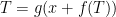 , where
  is the radiation’s temperature-independent component. That temperature-independent component may be, say, back radiation caused by carbon dioxide that we’ve placed into the atmosphere by burning fossil fuels.
 and
and  ? I don’t know. But let’s assume some functions that don’t ignore dependence on the entire temperature and observe how that constrains sensitivity. We’d expect temperature to be less dependent on temperature as temperature increases, and modelers who talk about things like tipping points obviously expect back radiation to become increasingly dependent on temperature as temperature increases. So let’s say for the sake of discussion that the functions take the following forms:

 ,
,  ,
,  are constants.
 is all the radiation,
  is the whole temperature, and
  responds to that whole temperature.
 ,
,  , and
, and  . If we employ the inverse function
  of the resultant relationship
  on Lord Monckton’s assumed “emission temperature”
  , we get a temperature-independent radiation component
  , which we’ll take as our value for insolation after albedo. If we then solve the feedback equation
  for that value we get
  . That is, this model does exhibit a “substantial feedback response”
  to the emission temperature: it exhibits the response that Lord Monckton says the mainstream climate models lack.
 of COGS-caused back radiation to the
  of insolation to obtain a higher value
  . Solving the feedback equation
  with this increased temperature-independent radiation component
  gives us Lord Monckton’s pre-industrial temperature
  .
. of “forcing.” Forcing is an initial radiation imbalance that would result from suddenly making a given CO2 concentration change. We make an estimate
  of the temperature change needed at the effective emission altitude to cause that radiation change, and we obtain the surface radiation change
  needed to cause the same temperature change at the surface. By solving
  we obtain a sensitivity
  .
.
If the models instead assume nonlinearity, they can instead arrive at their high sensitivities without ignoring the portion of temperature below some cutoff.
Let’s suppose for purposes of discussion that under the conditions modelers assume in this context the solution to the model equations results in some equilibrium relationship
Let’s also say that the radiation
What is the nature of the functions
and
where
Now, you may think that such relationships are much too simple and imply much greater sensitivity than the evidence supports. I agree; I don’t for a moment think that such relationships are valid. But that’s neither here nor there. What’s important to the present discussion is that they don’t ignore, as Lord Monckton contends that climate models do, the portion of the temperature value that’s less than some “emission temperature”:
Let’s suppose that
Since this model doesn’t lack that response, let’s determine whether recognizing that “substantial feedback response” has caused the model’s equilibrium climate sensitivity to be low. To do that we’ll first add
Equilibrium climate sensitivity is the change in equilibrium temperature caused by a doubling of CO2 concentration, and doubling that concentration is said to result in
By recognizing that the earth isn’t linear, in other words, climatologists are perfectly capable of arriving at a high sensitivity even if they take the entire temperature into account, i.e., even if their models provide “substantial feedback response.”
Of course, that doesn’t make them right. It merely makes Lord Monckton’s argument risible.
“If the models instead assume nonlinearity”
The feedback loop becomes non linear too. The earths remarkable stability says the earth operates in the low, linear portion of the loop gain, ie, CO2 has little effect.
The Born Liar, who seems more interested in doing me down personally and in an arrogant, sneering tone than in trying to attain the objective, scientific truth (perhaps because he is still smarting having been caught out in a malevolent lie on an earlier occasion) here recycles a defective argument that he had made in an earlier thread, but without being honest enough to say so, and without being honest enough to admit that he has now been compelled to tweak the numbers to try to produce a less implausible artificial scenario than his previous artificial scenario, and without being honest enough to admit that I had not derived the 255.4 K emission temperature by “reading” it, as he dishonestly suggests, but by calculating it from officially-published estimates of insolation and albedo, as explicitly set forth in the head posting. The Born Liar is also not honest enough to admit that my value of the emission temperature is not “assumed” but calculated, and not honest enough to admit that the term “emission temperature”, which he puts in pejorative quote-marks, is used frequently in the peer-reviewed literature, which is why I use it too.
So let us look at the Born Liar’s artificial scenario and do the math. He now apportions the 32.2 K difference between the 287.6 K temperature in 1850 and the 255.4 K emission temperature as follows: feedback response to emission temperature 15.2 K, directly-forced warming from the presence of the naturally-occurring, non-condensing greenhouse gases 8.9 K, and 8.1 K feedback response to that directly-forced warming. Using the defective official form of the zero-dimensional-model equation, his implicit feedback fraction, as far as the non-condensing greenhouse gases go, is 1 – 8.9 / (8.9 + 8.1) = 0.48, implying a Charney sensitivity of 2.1 K, right at the bottom end of the official CMIP3 and CMIP5 interval of Charney sensitivities. But he can only push the Charney sensitivity up this far by imagining that his 15.2 K feedback response to emission temperature is only 5.9% of it, while his 8.1 K feedback response to the 8.9 K directly-forced greenhouse warming is 91% of it. In short, he is trying to imply that if one corrects official climatology’s error in either not taking any account of the feedback response to emission temperature (in accordance with IPCC’s definition of a climate feedback) or taking only an inadequate account of it the nonlinearity of the system will be more severe, rather than less severe, than it is now in the uncorrected system. That is the central implausibility of many in his conclusion.
It is now time for the Born Liar to stop being arrogant, stop being vicious, stop being spiteful, stop describing results he does not understand as “risible”, and start doing some real work. Let him begin by finding some concrete examples of models or papers that make explicit and quantified allowance for the feedback response to emission temperature. When he has found them, let him explain why it is that such papers are incompatible with IPCC’s definition of a “climate feedback” as one which arises only in response to a change in temperature, rather than to a pre-existing temperature. Let him explain why it is that his scenario indicates a nonlinearity in the corrected system that is greater rather than less than the nonlinearity in the present system. Let him also justify the reasons for so strong a nonlinearity that the feedback processes in his scenario respond 15 times more enthusiastically to enrichment of the atmosphere with non-condensing greenhouse gases than to emission temperature.
And let him do all this politely, civilly, and in a spirit not of trying to find personal fault with me but of trying to attain the objective truth. If he will learn to behave in a civilized and scientific manner, and if he will cease his campaign of artful misrepresentations and start playing with a straight bat, I shall cease to call him the Born Liar,. Redemption is available to all who repent.
Joe
That is, although he pays lip service to nonlinearity, he bases his argument on the system’s being linear.
If the models instead assume nonlinearity,
You have picked up exactly the wrong end of the stick. But inadvertently you have identified the most interesting aspect of Monckton’s argument. Which simply amounts to a rediscovery of what the climate establishment have been trying to hide – Lorenz’s deterministic nonperiodic flow. Lorenz showed in 1962 that even a simply modeled climate system will never reach equilibrium. That with no change to external inputs the system’s state will always change and can never be characterised by a mean or equilibrium value.
What Monckton has now done is focus attention on the question of, in a climate system, what is equilibrium and stasis and what is perturbation from stasis? And the answer is simple and devastating. Equilibrium and stasis are nonexistent and meaningless concepts in climate. The fault that Monckton has exposed in climate science is far bigger than he realises. He has shown that the whole edifice of back radiation atmospheric modelling and CO2 warming is built on a vacuous foundation – on no foundation at all. At its heart are the impossible, nonexistent and meaningless concepts of equilibrium and stasis. It’s cute for you to be invoking nonlinearity now when talking about a paradigm and narrative built on equilibrium and stasis. These are not features of a dissipative open chaotic-nonlinear system characterised by feedbacks. The climate, that is.
The climate research community thought that they could just ignore Lorenz and he would go away. And it worked – as it always does. He – the person – did go away. But the theory he established didn’t go anywhere except to turn out to be not theory but fact.
Lorenz would have told them if they had listened that the climate is a far from equilibrium system in which stasis can never exist. But instead they built a climate theory on concepts of equilibrium and stasis. Considering the climate as a linear closed system, concepts of thermal balance, equilibrium and stasis are natural and compelling. But they are wrong and the entire theory and paradigm will have to be discarded.
You cant separate a static / equilibrium component and a perturbed / reactive component of the climate. If the system contains positive feedbacks then the whole system is excitable, just as negative feedbacks confer friction to the system. The system is dynamic and can’t be divided into parts where feedback operate and where they don’t. As Lorenz showed, such a system is always changing, in flux. It’s analogous to moving from algebra to Newtonian (OK Leibnitz too) calculus, where the meaningful values are instantaneous changes and rates of change, not static values.
This conclusion is very profound and thus can be arrived at from different directions. Lorenz found one – Monckton has found another.
As usual, Lord Monckton mischaracterizes things. I previously gave an example of how, without ignoring low-temperature feedback, climate modelers might generate high sensitivity and still match Lord Monckton’s numbers. With the head post here Lord Monckton appeared to change his numbers, so I changed the parameters to match the new numbers, just as one would expect climate modelers to tune their models to observations.
Yet, as is his wont, Lord Monckton implies that there’s something sinister in my doing so.
So what? I provided an example of how climatologists might arrive at high sensitivity without ignoring the “emission temperature.” What Lord Monckton basically observed is that I did that by making feedback per degree increase greatly with temperature.
Of course I did. If climatologists are going to get high sensitivity, that’s the only way. I don’t think sensitivity is high, and I don’t think the real-world relationships are what I put in that model. But if climate modelers think evaporation’s net effect (through clouds, greenhouse gases, etc.) is to warm the earth then it wouldn’t be too surprising for them to make this effect per kelvin greater at higher temperatures; that’s the way evaporation works. And the fact that enhanced higher-temperature loop gain would thereby emerge from the modelers’ resultant equations is no evidence that they ignored feedback at lower temperatures. It’s much more likely evidence that they thought, evaporation being what it is, that such feedback is much less in those regimes.
This confuses two things. One is whether the climate models make temperature-affecting things like back radiation, albedo, etc. responsive to temperature throughout the temperature range. To me Lord Monckton’s contentions that they don’t seems nearly inconceivable. The second is whether they call that response feedback. Apparently they don’t, but that’s merely a nomenclature issue; whether they call the response feedback has nothing to do with whether they implement it.
Unfortunately, the two issues keep getting conflated in these threads.
This is the second time Lord Monckton has recently perpetrated that slander at this site. So let me repeat what he calls a “malevolent lie.”
Among other evidence in a previous paperthat Lord Monckton had wandered in over his depth, he provided a “transience fraction” table purportedly derived from the Roe paper but indicating that a Roe-system step response would be lower at 25 years for modest positive feedback than for no feedback at all. Obviously, Roe said no such thing, so I wrote a post directed to some of the reasons why more information was needed about how he chose the transience-fraction values. But Lord Monckton turned down that request by merely repeating that he got them from Roe. What he calls a “malevolent lie” was my saying so.
Someone truly interested in the “objective, scientific truth” would simply show his work rather than whine about my not saying pretty please with sugar and honey on it when I pointed out the omission. But as far as I know he still has given no explanation of how he obtained such implausible values.
philsalmon:
Thanks for you conclusory assertions, but I see no reasoning to back them up.
Have a nice day.
Thanks. Very helpful.
Joe Born
I cited Deterministic Nonperiodic Flow, Lorenz 1962, thinking that the important theory and discovery in this paper regarding chaotic dynamics was common scientific knowledge. That is what citation is for.
https://journals.ametsoc.org/doi/pdf/10.1175/1520-0469(1963)020%3C0130:DNF%3E2.0.CO;2
But in an exercise in collective gaslighting, you and the climate community with you are trying to deny the existence of Ed Lorenz and of DNF 1963. And with good reason.
So I will repeat my arguments in case you missed them the first time:
1. Contrary to your stubborn denial, DNF1963 does exist.
2. The concept of equilibrium in climate dynamics is invalid since Lorenz showed that climate has never and will never attain equilibrium. It possesses the dynamics that it does on the basis of its being a far-from-equilibrium system.
3. The concept of perturbation from a (fictitious) equilibrium is invalid since there is no equilibrium from which to perturb, and in any case the system is endlessly perturbing itself.
4. A Lorenzian model of climate is one that has the fundamental property that it is always changing. Once this is understood, then the term “climate change” is emptied of meaning. “Climate” and “climate change” have the same meaning so “change” is a redundant tautology, the same as saying “the Catholic Pope”.
The use of the term “climate chage” is a statement of denial of or of ignorance of DNF1963 and its inescapable implications.
Phil Salmon
“1. DNF1963 does exist”
Yes, I’ve discussed it here.
“2. The concept of equilibrium in climate dynamics is invalid”
The concept is OK. It may not be attained.
“3.The concept of perturbation from a (fictitious) equilibrium is invalid”
The theory of feedback does not require perturbation from equilibrium, though a stable operating point is conceptually easier. It just describes what happens to perturbations. As to endlessly perturbing, many feedcack amplifiers are constantly responding to signals (eg telecom repeaters). Feedback analysis still works.
“A Lorenzian model of climate is one that has the fundamental property that it is always changing.”
It has the property that it is always evolving according to trajectories that lie on the attractor. But if the attractor shifts, that is something else. AGW moves the attractor.
philsalmon:
My response to you was perhaps too cursory. I don’t deny anything you say about chaotic systems.
I just don’t see how it’s germane to the question before the house, which is whether climate models’ hypersensitivity results from modelers’ failure to recognize various temperature-affecting quantities’ responses to temperatures below the “emission temperature.” The only arguments I’ve seen for that proposition are Lord Monckton’s inept math and irrelevancies such as how feedback is defined.
Yes, yes we can go off on tangents about sensitivity to initial conditions, strange attractors, etc., etc. But what I’m concerned about is that Lord Monckton has horned into that lawsuit with an appalling amicus brief that makes skeptics look like buffoons. Previously he was relatively harmless. Now he has become destructive.
The Born Liar lies again. He now tries to maintain that he made an undeclared alteration to his old argument to take account of some variations in my numbers. That, of course, is nothing but mendacity, for the head posting makes the point that our argument has come full circle, so that we end up with the feedback fraction 0.08 with which we started. Mr Born’s real reason for his undisclosed reworking of his numbers was that he had been humiliated by my pointing out that his earlier attempt had implied a Charney sensitivity not much greater than our own. And, even now, the best he can do is reach a Charney sensitivity of just above 2 K, which is right at the bottom of the models’ range.
He has utterly failed to provide any evidence even to the effect that the net feedback fraction will increase exponentially rather than remaining approximately linear or even declining. He has utterly failed to provide any evidence that – since such small net nonlinearity as may obtain in the feedback process is no less present under the present disposition than under our correction of it – our result will do anything other than greatly reduce equilibrium sensitivities.
All he has done – which did not need to be done – was to devise an artificial scenario bearing little or no relationship to the real climate, and then to show that under that manifestly absurd scenario the temperature feedbacks would somehow know that they should produce 15 times as much response per Kelvin to the presence of the non-condensing greenhouse gases as to the emission temperature. He has offered not a shred of evidence for or explanation of that startling discontinuity, which bears no relation whatsoever to the near-perfectly thermostatic behavior of the climate over the past 810,000 years.
The Born Liar has provided not a shred of evidence that the models take any account of the large feedback to emission temperature. So far, it is only I who have done that – and, even then, the paper I cited did not make any explicit statement that the additional temperature was a feedback response to emission temperature. He has now gone so far as to say he cannot quite believe that the models did not take the feedback response to emission temperature into account, which is perhaps a small step on his part towards the light. But, to everyone but a true-believer sullenly determined to adhere with naive faithfulness to the Party Line, it is surely obvious by now that IPCC’s definition of a “climate feedback”, recited in the head posting, precludes absolutely the assignment of any value to the feedback response to emission temperature; and, now that the Born Liar has had two failed attempts at producing scenarios that correct official climatology’s error, both of which implied Charney sensitivities very considerably below even the mid-range official estimate, and a fortiori still further below the foolish high-end estimates on which policies are based, it must now be apparent even to him that official climatology cannot possibly be giving due weight to the feedback response to emission temperature, for otherwise even its mid-range estimate would be absurdly excessive.
Mr Salmon’s most interesting comment deserves a considered response. I, too, am fascinated by Edward Lorenz’s great paper on deterministic nonperiodic flow – the paper (my edition of it is dated 1963) that founded what would later come to be known as chaos theory, though Lorenz himself did not use the term. Mr Salmon may perhaps also have read the paper by Giorgi (2005) on chaoticity in the climate, and perhaps also the magisterial and also delightful paper by Sir James Lighthill (1998) on chaoticity in the oscillation of a pendulum.
I have seen some arguments to the effect that the climate is not a chaotic object. However, it is plainly an object that behaves chaotically. As Lorenz’s title makes clear, the fact that an object behaves chaotically does not prevent it from behaving deterministically; but chaoticity makes the evolution of the object over time very difficult to predict. My favorite examples of this predictive difficulty are the Mandelbrot set, whose equation is remarkably simple but which constitutes the most complex object in all of mathematics, and the Verhulst population model, which is ordered until the population growth rate exceeds 3 by even the smallest fraction, whereupon its behavior is chaotic.
Mr Salmon is of course quite right that, provided that the index variable or variables is or are within the interval over which chaos reigns, all talk of an “equilibrium” is vain. However, I submit that it is permissible for official climatology to posit actually unobtainable equilibria as the start-point and end-point of a time-series evolution of the chaotic object that is the climate, and then to try to investigate the impact of anthrogenic influences on the closing equilibrium.
The point of our research is simply this: that one must take explicit account of the full feedback response to emission temperature: for it is a large response, accounting for some two-thirds of what is currently and erroneously thought to be the “natural greenhouse effect” caused by the presence of the non-condensing greenhouse gases. However, IPCC’s definition of a “climate feedback” makes no provision for this large feedback response, and, indeed, does its best to exclude it, so that that response can be quietly added to the far smaller feedback response to the presence of the non-condensing gases, thereby greatly inflating equilibrium sensitivity.
A Lorenzian model of climate is one that has the fundamental property that it is always changing. Once this is understood, then the term “climate change” is emptied of meaning.
Nope.
The Lorenz model is actually nothing but a model of Rayleigh-Bénard convection.
https://en.wikipedia.org/wiki/Rayleigh–Bénard_convection
Mathematically it’s a system of 3 coupled non-linear differential equations with 3 variables X,Y, Z and 3 parameters such as the Prandtl number. The parameters are constant quantities related to fluid properties and imposed boundary conditions such as the temperatures held constant on lower and upper plates. In Lorenz calculations they do not change as the dynamic system evolves and representative point (X,Y,Z) follows its trajectory on attractor.
As pointed out by Nick Stokes, the analogy with a specific climate is a specific attractor that corresponds to a specific set of parameters.
Climate change is thus a change in the attractor brought about by a change in the parameters of the non-linear equations. For instance in Lorenz model the imposed boundary temperatures or in climate the sun “constant” or atmospheric CO2 partial pressure.
This is in sharp contrast with a change in variables (X,Y,Z) that is the analogue of weather in a specific climate.
The concept of equilibrium in climate dynamics is invalid
It isn’t invalid.
Climate system is a dissipative structure and “equilibrium” just means that usually a steady state is reached where an essentially constant flow of energy traverses and dissipates in the system. In other words: energy in = energy out, when averaged over some period of time. Energy is just degraded, entropy produced in the system but there is no substantial accumulation or depletion of energy in the system.
Lord Monckton seems unable to refrain from falsehoods. First, he cannot possibly know why I changed the numbers. Second, the “Charney sensitivity” I reported last time was 3.25 K. Third, the value this time to account for his number change was 3.21 K. Moreover, I needed only change parameters if I had wanted even higher sensitivity values.
 and feedback function
  :
:
 ,
,  , and
, and 
 ,
,  , and
, and  ,
,
If anyone wants to see for himself who tells the truth, he can reproduce the calculations I described in the comment above. To that end I provide here values pulled directly from the computer, without truncation:
The (after-albedo) radiation absorbed by the surface:
The parameters for the open-loop function
Temperature before naturally occurring greenhouse gases (“NOGs”) or feedback: 255.4 K.
Temperature before NOGs, but with feedback: 255.4 K. + 15.20079 K = 270.60079 K.
Temperature with NOGs, but before feedback to NOGs: 270.60079 K. + 7.8141 K = 278.4149 K.
Temperature with NOGs and feedback: 278.4149 K. + 9.184937 K = 287.599824 K.
Temperature with CO2 doubling but without feedback to CO2 doubling: 287.599824 K + 0.9815485 K = 288.5813721 K.
Temperature with CO2 doubling and feedback: 288.5813721 K + 2.231325 K = 290.812697 K.
“Charney sensitivity,” i.e., the difference between the temperatures with and without CO2 doubling: 290.812697 K – 287.599824 K = 3.212873 K. That is, not Lord Monckton’s “2 K.”
Now the parameters that I used last time in order to produce Lord Monckton’s previous number (244.6 K) for the temperature before NOGs or feedback:
which after somewhat different intermediate values yielded a “Charney sensitivity” of 3.24344 K. (It appears I made a transcription error last time; I reported 3.25 K.)
So, as usual, what Lord Monckton says isn’t even within shouting distance of the truth.
As usual, Lord Monkton spouts irrelevance. I had never contended that I had any evidence for an increasing “feedback fraction.” In fact, I explicitly stated just the opposite:
And I then demonstrated that if modelers thought temperature-affecting quantities’ sensitivity to temperature increased disproportionately with temperature—as they likely believe in light of evaporation’s response to temperature—then, contrary to what Lord Monckton continues to contend, they don’t need to ignore responses to temperatures below the “emission temperature.”
Lord Monckton keeps running from that point by filling these threads with falsehoods, irrelevance, illogic, and sophomoric name-calling. He gives us bombast instead of substance, logorrhea instead of logic, and falsehoods instead of truth.
Nick, Christopher, Joe, gammacrux
I’m grateful for your replies to my amateurish contribution on my favourite chaos theme (I’m a marine biologist turned radiobiologist taking an interest in climate). I probably overstated my case for rhetoric effect.
Nick – I appreciate your acknowledgment of attractors – but I don’t see much of that language in the IPCC and climate literature. I still feel it needs to move more center stage, in many scientific fields not only climate.
Christopher – thanks for the perspective and useful references. “Deterministic” was I guess used by Lorenz in the mathematical sense. That chaos can be represented mathematically makes it deterministic in an ideal Laplacian manner. But the knowledge of initial conditions required for such predictiveness is impossible so in practice deterministic becomes non deterministic. I think the really interesting and important thing about Lorenz’ simulation, on almost the world’s first computer (aside from Turing’s WW2 colossus), is that the system changes by itself without forcing from outside.
Joe
I’m a mere biologist and can’t do complex maths. Chaos literature is full of scary formulas which I ignore entirely and just look at the pictures. (I can just about understand Feigenbaum’s quite simple conditions for chaotic bifurcation.) Monckton’s prose description of his essential case did however seem to make sense. The emission temperature is the “equilibrium” temperature with a warming effect of CO2. Then there is an additional temperature increase caused by a perturbation in the form of an incremental addition of more CO2. The question appeared to be – do feedbacks in the system apply only to the incremental temperature increase from the incremental CO2 addition, or do they apply to all the temperature difference between an “equilibrium” entirely without CO2 and the final temperature with “baseline” and incremental CI2 added. Put in those terms, it seems reasonable that feedbacks should indeed apply to all the temperature elevation caused by CO2. Critics have challenged CM saying “you can’t apply feedbacks to the equilibrium situation, only the incremental”. But even the additional warming from the incremental CO2 still leaves you at an equilibrium. So what indeed is the difference and why discriminate between the two?
(This is how biologists try to verbalise such questions – avoiding maths but still considering ourselves scientists.)
I felt that a chaos perspective would have feedbacks operating instantaneously on the system at all times whatever its state – since the state would always be changing.
gammacrux
The Lorenz model is actually nothing but a model of Rayleigh-Bénard convection.
What’s wrong with that? What is climate other than turbulent flow of water and air?
philsalmon
What’s wrong with that? What is climate other than turbulent flow of water and air?
Nothing is wrong with that. My remark was just to provide the proper context of chaos theory of dynamic systems and emphasize the origin of your misunderstanding, namely the major difference between parameters and variables in that theory.
Yet, that said, climate is actually much more than just a problem of fluid mechanics or evolution of a dynamic chaotic system. It involves a lot of so-called emergent phenomena that definitely cannot simply be inferred, deduced or anticipated from first principles of physics. They must be discovered and studied by observation and experiment.
Biology for instance is clearly involved in cloud formation, for instance with the aerosols produced by marine life and living creatures are precisely the most remarkable emergent phenomena in nature.
So to come back to the concept of “equilibrium”, I can’t see why you dispute the validity of that concept for the climate system while as a biologist you certainnly readily admit it in the case of a living creature such as a grown-up animal. In both case a steady state may eventually be reached where there is nothing but a constant flow of energy that just traverses, degrades and dissipates in the system. No net energy accumulates in or flows out of the system, i. e. the climate doesn’t warm or cool on one hand and the animal neither changes its temperature nor gains or loses weight on the other hand.
The Born Liar provides a Gish gallop of numbers artfully intended to conceal the fact that the equilibrium sensitivity inherent in those numbers depends upon the feedback fraction 1 – 8.9 / 17 = 0.48, giving Charney sensitivity <2,.1 K. And he still provides no explanation of how it is that after correction of official climatology's large error Charney sensitivity remains unaltered at the current official mid-range estimate. Fortunately, very few are paying attention to the Born Liar's expatiations, since he cannot conceal his malevolence. His, therefore is not trustworthy testimony, on grounds of prejudice. It may be disregarded.
Monckton of Brenchley April 7, 2018 at 8:31 am
It is now time for the SNIP Monckton to stop being arrogant, stop being vicious, stop being spiteful, stop describing results he does not understand as “risible”,
And let him do all this politely, civilly, and in a spirit not of trying to find personal fault with me but of trying to attain the objective truth.
Corrected.
Phil. April 10, 2018 at 9:49 am
“Monckton of Brenchley April 7, 2018 at 8:31 am
It is now time for the SNIP Monckton to stop being arrogant, stop being vicious, stop being spiteful, stop describing results he does not understand as “risible”,
And let him do all this politely, civilly, and in a spirit not of trying to find personal fault with me but of trying to attain the objective truth.”
Corrected.
Interesting that my strike-through of Monckton’s insulting remark is deemed worthy of snipping by the Moderator whereas the original insult by Monckton is not and he continues to use it!
Let us conduct a simple Gedankenexperiment, running in reverse the model of Lacis et al. (2010), who found that
I’m a big fan of Christopher Monckton of Brenchley, he’s been a wealth of information and a voice of sanity in this debate. But I question this approach.
The fatal flaw (IMHO) is that we have no way to determine if Lacis et al is accurate. He didn’t test an actual earth, he modeled it. If the model was wrong, then his result, and Christopher’s Gedankenexperiment which is arrived at by running it in reverse, is also wrong, is it not?
I was thinking this as well.
I agree. MB needs to keep it simple, and that whole analysis is just muddying the waters.
Steve Richards is correct and, with respect, David Hoffer has perhaps not understood the limitations of a Gedankenexperiment. I had hoped, in the head posting, to make it clear that I considered Lacis (2010) to be wrong, as my own reverse running of their experiment plainly demonstrated. I had also made it clear that other values of – for instance – albedo and hence of emission temperature might be chosen, though they would not make any difference in the long run.
A Gedankenexperiment is an illustrative example: nothing more. if it doesn’t work for you, no matter: the underltying math still ineluctably requires a substantial feedback response to emission temperature that IPCC’s definition of a “climate feedback” altogether rules out: and, if that response is properly taken into account in its own right rather than being arbitrarily counted as part of the far smaller feedback response to the non-condensing greenhouse gases, equilibrium sensitivity must fall, and fall substantially.
if it doesn’t work for you, no matter
It doesn’t matter if it works for me or not. The alarmist argument has been without merit or evidence for many years. It has been running on emotion and hype for as long as I’ve been paying attention. Finding fault with one paper that may or may not be correct doesn’t persuade the common man.
Mr Richards has it exactly right. Lacis et al. are the nest of vipers at NASA who have been profitably peddling extremism as though it were science. I have taken their paper as an illustration of the error that has been made – but it is only an illustration. It should surely be possible for Mr Hoffer to read the head posting and appreciate that practically nothing in our argument would fall away if we ignored Lacis altogether.
The central question remains – a question that all the true-believing climate fanatics here have been entirely unable to answer in any intelligent fashion. How is it that inanimate feedback processes are capable of distinguishing between emission temperature and the small enhancement of it represented by the direct warming from the presence of the naturally-occurring, non-condensing greenhouse gases, so that they react little if at all to the former but very strongly to the latter?
If Mr Hoffer does not grasp just how fundamental this point is, and just how little it depends on anything in Lacis et al., then my powers of exposition are less than I had hoped.
It should surely be possible for Mr Hoffer to read the head posting and appreciate that practically nothing in our argument would fall away if we ignored Lacis altogether.
Then may I respectfully suggest that you make the argument in just that fashion.
Mr Hoffer need only remove those parts of the head posting that mention Lacis’ paper. The remainder will provide quite enough to chew on.
The whole basis of Moncktons work in this post is to assume that all of ‘official’ climatology is correct and show one major ‘official’ fault with its workings.
If this fault is agreed then it dismantles the climate scare.
No more no less.
Is Lacis et al correct or incorrect? It does not matter other than the fact it is:
a) Is lauded by ‘climatologists’;
b) adopts all current climate theory.
Show the major flaw and the walls fall down.
“At the 255.4 K that would prevail at the surface today without greenhouse gases or feedbacks…”
Without greenhouse gases there would be no cloud albedo. The zero albedo black body figure for the hypothetical uniformly heated globe is 394*0.25^0.25 = 278.6K. For the oceans with a 0.06 albedo that would be reduced to 274.32K or 1.17°C.
“Without greenhouse gases there would be no cloud albedo.”
No you could have water vapour without CO2. The real problem is that the earth started with CO2 and the water came later. the analysis should g o right back to the beginning 4.6 billion years ago. All Monkcton is saying is that there has to be a forcing of water vapour that is always much greater than the forcing of CO2. He rightly points out that the climate models have the sensitivity equation backwards by having a large CO2 forcing at the 1850 year which should have been a large cloud and H2O forcing which then drives the smaller CO2 forcing. Actually Moncktons 1850 bar graph should be (based on his brief submission to the court) 8K for clouds 23.4 K for H2O and 0.8 for CO2. Both Monckton and the climate models attribute a much too large temperature forcing caused by CO2.
Irrelevant to my point.
Yogi Bear appears not to have read the head posting. So let me review the necessary elementary climatology,. First, emission temperature is a function solely of insolation and albedo. If the albedo is today’s 0.293, then the emission temperature will be 255.4 K, and that temperature will obtain at the Earth’s surface. However, there cannot be an albedo as high as 0.293 without clouds and ice, implying the presence of water in various forms, not the least of which is water vapor. Water vapor is a condensing greenhouse gas, and its existence provides the mechanism of a feedback process. That feedback process responds to emission temperature, so that the Earth’s surface temperature will be significantly higher than the emission temperature, even before taking any account of the presence of the non-condensing greenhouse gases.
Monckton appears not to have understood my quote of his, which claimed:
“At the 255.4 K that would prevail at the surface today without greenhouse gases or feedbacks…”
An albedo of 0.293 does naturally imply clouds and water vapour, which is the larger part of the so called greenhouse effect, so the surface temperature would have to higher than 255K without greenhouse gases or feedbacks according to your definition of water vapour being a feedback.
But the water vapour is not a positive feedback to 255K, it’s a thermal reservoir that moderates the diurnal temperature swings like the oceans do. And has enough thermal capacity to enable strong poleward heat transport, as a negative feedback to net changes in total climate forcings.
Yogi Bear is entitled to his opinion about what does and does not constitute a temperature feedback. However, in the head posting we have made it explicit that, for the sake of argument, we have accepted for the sake of argument all of official climatology except what we can prove to be wrong. And, whether Yogi Bear likes it or not, the water-dependent processes in the climate are represented as feedbacks in official climatology. That is precisely how we have represented them, and that is precisely why there is a substantial feedback response to emission temperature – a response that IPCC’s definition of a “climate feedback” does its very best to exclude from the account. In that respect, IPCC is simply wrong.
It’s not a feedback, it’s a longwave clawback from cloud albedo losses, and from near infrared losses by water vapour.
Yogi Bear is entitled to his opinion that the water vapor feedback is not a feedback. But in the head posting I have accepted ad argumentum all of official climatology except what I can prove to be incorrect, and official climatology treats the water vapor feedback as a feedback, denominated in Watts per square meter per Kelvin of the temperature that induced it.
‘Official climatology’ says that Earth’s surface temperature without all greenhouse gases and water vapour is 279K (minus the surface albedo) and not 255K.
“official climatology treats the water vapor feedback as a feedback”
To net changes in surface temperature of course. You cannot legitimately call it a feedback to absolute temperature when it physically substantially reduces maximum daytime land surface temperatures.
Yogi Bear is confused. The water vapor feedback delivers a feedback response to any temperature that is present, whether that temperature be the input signal from the Sun or some amplification thereof forced by the presence of non-condensing greenhouse gases.
“Yogi Bear is confused.”
No you are.
“The water vapor feedback delivers a feedback response to any temperature that is present, whether that temperature be the input signal from the Sun…”
Nonphysical word salad. Water vapour inhibits direct surface heating by the Sun as it absorbs considerable amounts of solar near infrared.
“…or some amplification thereof forced by the presence of non-condensing greenhouse gases.”
You don’t know that a net increase in non-condensing greenhouse gas forcing causes a positive water vapour feedback.
Yogi Bear is even more confused. If the water vapor feedback is negative, as he appears to be suggesting, then our result is demonstrated a fortiori. However, ad argumentum we have accepted all of official climatology except what we can prove to be wrong, and official climatology considers the water vapor feedback to be positive. It does not care whether it is responding to the emission temperature or to the addition to emission temperature caused by adding in the non-condensing greenhouse gases, or to the further temperature increase caused by anthropogenic forcings. It is positive in respect of all of these. However, it is not very strongly positive.
Standard climatology sensibly does not consider water vapour a feedback to emission temperature.
Fourth draft posted. Why?
Write it up, Monckton, submit it for peer review. Quit trying to …what are you trying to do, anyway? Convince more people of this egregious error you go on and on about? If they aren’t convinced yet, why would it work now? How have you dealt with the problem that to have a feedback there has to be initial change? You haven’t, so it’s all a waste of time. Try publishing it and see how far you get, since you’re such a superior scientist. Oh, yeah, you aren’t a scientist. No wonder you don’t get it. Funny how so many skeptics think you have expertise, often the same ones who think that those who went through a decade of post-secondary education and devoted their professional lives to science are so brainless that none of them have thought of looking at natural variation for a explanation for climate change.
And why do you focus on this one paper by Lacis, et al., anyway, if all climate change models by the AGW consensus community suffer from the same error?
You should stuff yourself in a box. According to climatologist orthodoxy your 98.6F body temperature should generate 525+262.5+131.25…=1050 W/m^2 or 204F, and you’ll fry.
That didn’t happen? Lucky you. Then how can you believe climate junk science? Oh yes, you’re a fool, that’s how. You can’t understand the trick played on you by liars who pose as scientists.
Zoe,
That would depend on how well insulated the box was and if you continued to generate heat. If you
were in a box composed of silica aerogel surrounded by a vacuum and had some way of eat then you
would fry.
Germ,
Kristi’s body continually generates heat for days. She can be insulated in solid co2 to emulate extreme co2 atmosphere. WUWT is an infamous source of insight that cooler insulators heat a warmer source, so she should fry, not freeze.
Fortunately, “climatologist orthodoxy” is not nearly as simplistic as you pretend.
” You can’t understand the trick played on you by liars who pose as scientists.” I guess you don’t see the irony in this.
Oh, yeah, you aren’t a scientist
≠========
Drivel. Mathematicians are scientists. Mathematics is the language of science.
As the saying goes: all mathematicians can do science, but not all scientists can do math. Nowhere is this more evident than climate science.
Monckton a mathematician? Does he have a degree I don’t know about, one apart from classics and journalism? Just because someone can do math doesn’t make him a mathematician.
What saying? Mathematicians are not all scientists, although the two fields may collaborate, and climate science is an instance of that. However, mathematicians are not necessarily trained in the methodologies of science.
Fredberple,
It is off topic but Mathematicians are not scientists. Numbers are social constructs and do not
exist in reality but rather follow whatever rules we make up. Some of those roles are amazingly
good models for reality but others aren’t. Some applied mathematicians do science but many others
do amazing research in topics like number theory but they are certainly not doing science.
Germonio appears to think that those of us who study number theory are not doing science. To imagine that pure mathematics is divorced from science is a common and elementary misconception. For instance, the Boolean algebra used in the logic circuits of computers originated in number theory. Even the use of propositional calculus to improve railroad timetabling on busy routes comes from number theory. It was from number theory that many of the fundamental constants of mathematics were derived. And who would have thought that a simple result in probabilistic combinatorics – another branch fo pure math – could be turned into a pair of award-winning, best-selling jigsaw puzzles with million-dollar prizes?
The division between pure and applied math was always to some extent artificial. It is now rapidly disappearing.
Monckton wrote: “Germonio appears to think that those of us who study number theory are not doing science.”
Mathematicians and scientists have different ways of thinking. Scientists start with hypotheses and attempt to DISPROVE them through experiments. Those hypotheses that survive extensive testing become theories. The predictions of well-tested hypotheses can be trusted even if the theory is later revised – when those predictions are within the scope of the theory that has been well tested.
In mathematics, you start with a set of axioms and deduce as much as possible from them. There is little emphasis on testing axioms to see if the deduced mathematics tell us anything useful about the real world. Roe set out some axioms for feedback analysis of climate. You use those axioms to make deductions about amplification of warming. It doesn’t make any difference that Roe requires you to use information from climate models that you don’t believe in. Roe’s axions require a reference state. One version of Roe’s deduction is limited to linear feedbacks, while another version deals with non-linear feedbacks. Unfortunately, you don’t have the data to apply the non-linear version, so linearity becomes one of your axions – not a hypothesis that must be proven to be correct.
A few videos on Youtube show Feynman discussing the difference between mathematicians and physicists.
Frank does not appear to understand that mathematics – which is the language of the sciences – uses all of the methods of applied science and then some. Not the least of the weapons in the arsenal of mathematics is formal logic, in which I have no little training. One of the logical methods of formal demonstration or absolute proof is known as demonstration by contradiction. This method originated with Socratic elenchus, where the great philosopher would take his opponent’s proposition and draw conclusions from it that were agreeable to the opponent. He would then advance a proposition of his own, with which the opponent was likely to agree. When the opponent agreed, Socrates would draw conclusions from the second proposition, and the opponent would agree to them. Then Socrates would point out that one of the conclusions from the second proposition was incompatible with one of the conclusions from the first. If elenchus is deployed correctly, the opponent is left with no choice but to abandon his original proposition,.
Now, control theory contends that even an unamplified input signal will induce a feedback response provided that nonzero feedback processes are present,. This is long and well established, and we tested it empirically at a government laboratory just to make sure.
However, IPCC contends that an unamplified input signal cannot induce a feedback response. Either control theory is correct or IPCC is correct, but not both at the same time.
It is easy to see, using the corrected form of the zero-dimensional-model equation, that IPCC’s definition of a climate feedback is incorrect in that it limits a feedback response only to a perturbation in an original temperature, rather than also to that original temperature itself.
Silber
“How have you dealt with the problem that to have a feedback there has to be initial change?”
All Monckton is saying is that it is the climate models have the forcing built in. He is only ascribing the forcing that the climate models even in 1850 have built in. There has to be some because there was always CO2. There always is a feedback mechanism working. If you were a mathematician Kristi you would have understood that.
“How have you dealt with the problem that to have a feedback there has to be initial change?”
=====!!
Feedback operates on both AC and DC. When the sun warmed the earth from 3 K to 255 K that evaporated water which is the feedback that further warmed the earth. The 255 K temperature today keeps some amount of water in the atmosphere which warms the earth. Itbis this specific warming that has been overlooked in the analysis of climate feedback.
Silver: “How have you dealt with the problem that to have a feedback there has to be initial change?”
Every 24 hours there is a chain temperature. That should be enough to get the ball rolling, no?
*change in”, not “chain”
Of course there are feedback mechanisms. Monckton is not just saying that climate models have the forcing built in, he is changing the math, saying that there is feedback associated with a state, a temperature. Haven’t you been following the argument? Delta T is not the same as T.
Are you a mathematician, Alan? I’d like to have a trained, experienced mathematician explain how this is possible.
Silber says I have “changed the math”. If only it would read ch. 3 of Bode (1945), the standard textbook, it would rapidly discover not only that the corrected form of the zero-dimensional-model equation is what I say it is: it will see a formal proof of exactly how that equation is derived. There is nothing new in our math: what is new is our exposure of the fact that climatology has not made due allowance for the feedback response to emission temperature – a response that can be calculated by using the corrected form of the zero-dimensional-model equation.
Silber whines that there have been four articles in this series. But Silber is not obliged to read any of them, so why whine? If Silber had read the head posting instead of whining about it, Silber would have learned that I have provided a formal demonstration that there must be a feedback response to any temperature in the presence of at least one feedback process.
Silber describes me as a superior scientist and then as not a scientist at all. Perhaps Silber would like to decide upon one or the other viewpoint: they are mutually incompatible.
Silber then perpetrates the argumentum ad verecundiam by imagining that my distinguished co-authors lack the certificates of due Socialist training in climatology that I have at no time pretended to possess.
Finally, Silber asks why I focus on one paper, when I cited several, taking the one paper as the basis for an illustrative Gedankenexperiment. That is a standard method in the philosophy of science, a topic that formed part of my instruction at Cambridge (and I even have a certificate of appropriate Socialist training in Classical architecture, which embodied many ancillary elements such as the philosophy of science as well as the uses of early mathematics).
Silber is perhaps better at Socialist sneering than at science.
Monckton, you have no made any formal demonstration of anything. You have created a whole new
equation
T= T_ref/(1-f)
that superficially looks like Roe’s
Delta T = lambda_0 Delta F/(1-F)
but in fact is completely different and there is no logical way you can derive your equation from the
correct equation in Roe 2009. Simply stating that it is the correct equation is not sufficient.
Whining? That’s a laugh.
I corrected myself – of course you are not a superior scientist, you are no scientist at all. Perhaps you haven’t professed to scientific expertise; why, then, do you feel qualified to say real scientists are unquestionably wrong? Why haven’t you corrected those in the media who have made the mistake of saying you are an expert?
What the eff has this to do with socialism? That’s a classic denier move: attach a political ideology to a scientific theory in order to impugn those who have developed it or believe it. It has nothing to do with the quality of the science, which should never be viewed through the lens of politics. It’s the results of science that are used in policy-making, not policy that determines the science. The latter is an accusation oft made about “consensus” scientists, while the influence of politics on contrarian scientists is conveniently ignored.
Monckton, you are completely wrong about me being a socialist, not that it’s any of your business. The fact that you say such a thing is all the more reason for me to distrust your ability to view climate science from a scientific standpoint, rather than a political one. So much do you desire to “win,” you bring up personal issues that have nothing to do with the subject.
I don’t trust you, Monckton. Can you explain why the House of Lords had to issue an official statement that you never were a member? Why have scientists issued statements saying you misrepresented their work?
(If this is a paper written with co-authors, why aren’t their names in the by-line here? Why do you say “I did…” rather than “we did…”?)
” Most of those who have tried to dismiss our result in these threads know perfectly well that we are in substance right, and no amount of dressing up the actually very simple argument in other clothing would make any difference. These are not people in search of the truth: they are totalitarians wedded to the Party Line for good or ill. In due course we shall find a reasonably serious climate journal to publish our result, which will gradually become well enough known that no one will be able to ignore it, however uncongenial the true-believers may find it.”
Another convenient assertion that is not based on evidence. If argument from reason fails, attack the characters of those you can’t convince. It’s an old propaganda ploy; too bad so many people still fall for it.
(Please refocus onto the topic itself) MOD
Silber now reveals itself as a totalitarian by the use of the contemptible word “denier”. I do not care whether it calls itself a socialist or a marxist or a maoist or a communist or a fascist: it is a totalitarian. For none but a passionate adherent of some rigid Party Line or another would use the deliberately loaded word “denier” of someone who, like me, has stated explicitly in the head posting that he has accepted for the sake of argument all of official climatology except what I can prove to be wrong.
Germonio says that Roe’s form of the zero-dimensional-model is correct. Well, gee, get with the picture. That point is made in the head posting, which says that one can of course use that form of the equation without much error – provided that one has first made due allowance for the large feedback response to the input signal, which, in the climate, is emission temperature. The corrected forms of the equation presented in the head posting made that adjustment.
“Try publishing it and see how far you get, since you’re such a superior scientist.”
Well, he has submitted it to one journal, but the reviewers are giving him a hard time.