Guest essay by George White
Feedback is the most misunderstood topic in climate science and this misunderstanding extends to both sides of the debate. This is disturbing because the theoretical support for substantial warming cause by man’s CO2 emissions depends exclusively on the ability of positive feedback to amplify something small (3.7 W/m2 of forcing from doubling CO2) into something large (a 3C surface temperature rise).
What makes a 3C temperature increase relatively large compared to the forcing asserted to cause it is the difference between the equivalent emissions of a black body surface at the approximate average temperature of the planet (287K) and the equivalent emissions of a surface 3C warmer. Based on the Stefan-Boltzmann Law, the difference in equivalent emissions exceeds 16 W/m2 and for that surface to emit this much more, it must be receiving an equal amount. Independent of the specific origin of the more than 12 W/m2 of required surface input in excess of the 3.7 W/m2 of input forcing, the amplification required exceeds a factor of 4. One thing that’s clear is that the atmosphere has no internal sources of power, thus all of the power driving the 12 W/m2 of additional surface emissions must be coming from feedback. This fact alone is sufficient to falsify claims of a high sensitivity since it’s impossible for 3.7 W/m2 of stimulus entering a passive system to result in more W/m2 of feedback than it provides as input unless Conservation of Energy is violated. Climate science obfuscates this contradiction by considering only temperature and not the equivalent emissions of a temperature, thus a sensitivity of 0.8C per W/m2 sounds plausible, yet in terms of joules, 4.3 W/m2 of incremental surface emissions per W/m2 of forcing does not, especially considering that each W/m2 of incident solar energy results in only 1.6 W/m2 of net surface emissions.
Theoretically, positive feedback can provide the required amplification, but only if the system being modeled conforms to the many assumptions that predicated Bode’s control theory, originally developed in the 1940’s as a tool for designing linear amplifiers using vacuum tubes.
Hansen was the first to apply Bode’s analysis towards quantifying climate system feedback in his 1984 paper. Schlesinger quickly followed with a paper to ‘correct’ some of Hansen’s errors but actually made it worse. This faulty analysis has been canonized by the IPCC since AR1 and the few related papers that followed simply restate Schlesinger’s analysis using different variable names. An example is Roe’s 2009 paper on climate feedback which will be referred to below.
While Bode’s analysis provides the framework to achieve the required amplification, it can only do so under the specific conditions outlined in the first two paragraphs of his book. One of these conditions is the requirement for linear behavior between the input and output of the modeled network and another is the presence of linear vacuum tube elements with an implicit power supply that provides active gain which add energy to the output above and beyond what’s supplied by the input stimulus.
It should be self evident that the Hansen/Schlesinger mapping to Bode violates both of these preconditions. First is that the input to the feedback network is forcing, expressed in W/m2 while the output is in temperature, expressed in degrees K and that the relationship between W/m2 and degrees K, as given by the Stefan-Boltzmann Law is very non linear. When the relationship between the input and output of an amplifier becomes non linear, Bode’s formulation no longer applies and the gain becomes a function of the input rather than being strictly a function of the open loop gain and feedback. An example of this is when an audio amplifier starts to clip. The open loop gain and feedback remain constant, yet the closed loop gain steadily decreases as the input increases.
If a stimulus is applied to a complex, yet completely passive RLC circuit, all the nodes will wiggle, but this can never be considered equivalent to the behavior of an active system. Bode’s assumption of active amplification is not relevant to the climate either. Many confuse the dynamics of weather as an indicator of an active system, but in the context of Bode, active and passive have very specific meanings. Passive means that there are no other sources of input other than the stimulus, which for the climate is the W/m2 of forcing arriving from the Sun, while active means the system has powered gain driven by an implicit, internal power source. An important result of Bode’s analysis is that a passive system is unconditionally stable which precludes the possibility of runaway positive feedback.
The difference between a passive system and an active system is like the difference between manual steering and power steering. Manual steering is a passive system that achieves force multiplication (gain) by a combinations of gears, levers and pivots as energy is conserved between the steering wheel and the tires. Power steering is an active system that positively reinforces arm muscles by adding energy to the system from a hydraulic power source driven by the engine. The climate is a passive system that manifests surface temperature amplification by delaying surface emissions and returning them to the surface some time in the future where they are combined with new incident power from the Sun. It’s these joules of energy being delayed and returned back to the surface that comprises the physical manifestation of climate system feedback. This feedback is tangible, which for the climate is expressed in W/m2 which are added to the new input from the Sun also quantified as W/m2. Watts are joules per second and first principles requires joules to be conserved.
Bode’s feedback model removes the requirement of Conservation of Energy between the input and output of the system. This is the result of assuming an external power supply will provide as much output as required. This isn’t valid for a passive system like the climate where solar input is the only source of power and thus COE must be accounted for. Unlike an active amplifier which measures the input and feedback to determine how much output to deliver from an unlimited source, a passive system consumes its input and feedback to produce its output. Disconnecting the input and output from the requirements of COE makes sensitivities that violate COE seem plausible and this is the only reason that such an unreasonably high sensitivity can be accepted. When COE is added to the analysis, the maximum possible sensitivity becomes less than the lower limit claimed by the IPCC.
Technically speaking, the model proposed by Hansen called the system input a change in forcing and its output a change in surface temperature. For the linear systems modeled by Bode’s equations, the absolute and incremental gain are the same and independent of the magnitude of the input or output. For the climate system feedback model, this is an invalid assumption owing to the non linearity between W/m2 of input and degrees K of output, where the ratio of a change in output temperature per change in input forcing depends on the starting temperature. To get around this, it’s asserted that the system is approximately linear, but the feedback formulation sets the reference temperature to 255K and while the relationship between power and temperature is approximately linear on either side of 255K, the current surface temperature of 287K is too far from the reference for the assumption of approximate linearity to be approximately true.
The reason its been so hard for climate science to get this right is that there are many co-dependent and reinforcing errors in the mapping from Bode to the climate system which confuses many into thinking that the model is reasonable. However; without these errors, Bode’s model simply can not support the required amplification. Without this support for substantial climate change caused by man, the IPCC and the self serving consensus driven by its reports collapses and to many on that side of the argument, this is an unfathomable consequence, especially given the political ramifications.
In addition to failing to honor the prerequisite assumptions made by Bode, there are other errors regarding how Bode’s variables were mapped into climate related variables. This led to an arithmetic error that provided faulty support for a potentially high sensitivity which was never questioned due to confirmation bias. This arithmetic error has to do Hansen’s failure to understand the difference between the what Bode calls the feedback fraction and what he calls the feedback factor and this 3 decade old error is still with us today.
The feedback fraction is the fraction of output fed back to the input and is a dimensionless fraction between -1 and 1 spanning a range from 100% negative feedback to 100% positive feedback. The 100% limits arise because you can not feed back more than is coming out of the system in the first place.
Bode defines the feedback factor as the reduction in the open loop gain that arises as the result of feedback. This arises from Bode’s gain equation which he states as,
ER = E0 μ/(1 – μβ)
Where E0 is the input to the system (forcing), ER is the output of the system (the surface temperature), μ is the open loop gain (reference sensitivity, λ0 per Roe, 2008) and β is the feedback fraction which corresponds to feedback coefficients expressed with units of W/m2 of feedback per degree K. Bode labels the closed loop gain eθ which is calculated as eθ = ER/E0 = μ/(1 – μβ) and calculates the feedback factor as eθ/μ = 1/(1 – μβ) which is the reduction in μ that results from the application β. The most important aspect of this equation is the μ on both sides of the equals sign. Bode then makes a simplification assuming that μ >> 1 and β < 0, both of which are true for linear amplifiers and asserts that μβ by itself can also be considered the approximate ‘feedback factor’. Modern amplifier design ignores this altogether as the effective μ of modern amplifiers is on the order of many millions and as μ approaches infinity, μ/(1 – μβ) approaches -1/β (the feedback fraction) and the feedback factor becomes infinite.
To adjust the gain equation for COE, the power applied as feedback, Erβ, must be subtracted from the output since feedback power can not also contribute to the available output. The gain equation that is applicable to the climate becomes,
ER = E0 μ/(1 – μβ) – Erβ
Climate science incorrectly considers λ0 times an empirical coefficient, c1, as the metric to quantify feedback, considers their product to be equivalent to Bode’s μβ and calls this the ‘feedback factor’. Again, Bode’s assumptions were not honored since the climate system μ is very close to 1, and in fact is exactly 1 for an ideal black body, thus the feedback factor would really be 1 – λ0 c1. While a compensating error added the 1 back to the equation, it didn’t fix the misunderstanding that led to the arithmetic error in the first place.
The arithmetic error arises when to get the units to line up and ostensibly conform to Bode, Roe defines the feedback factor f = λ0c1 (per Hansen and Schlesinger). If the sum of the input and feedback (the input to the gain block) is J, the output of the gain block is J*λ0. Roe’s assignment of the feedback factor infers that that c1 = f/λ0. Multiplying the output of the feedback network by f/λ0 (c1) produces a feedback term equal to Jλ0f/λ0. The λ0 cancels leading to a feedback term quantified as Jf, where f becomes equivalent to Bode’s β when μ is 1 and quantifies both the fraction of output and the fraction of J returned as feedback. The specific arithmetic error is assuming that the open loop gain is both λ0 and 1 at the same time. This is illustrated in figure 1.

 |
‘
Figure 1
To illustrate the problem further, what μβ is actually quantifying is the post feedback influence of the input of the gain block, J, since the μ term amplifies the input while β takes a fraction of it and returns it as feedback. Conventional climate system feedback assumes that μβ is quantifying the effect feedback has on the output which is only true when μ is 1 and the input and output of the gain block are the same. A more accurate block diagram that represents the consensus climate science feedback model is shown in figure 2.
 |
Figure 2
Since the relevant open loop gain is a dimensionless 1, the output of the feedback network must be dimensionally the same as the input otherwise the input plus some fraction of the output can not be summed. The result is that what climate science calls the pre-feedback sensitivity, or the open loop gain, λ0, is no more than a scale factor applied to the required output in W/m2 converting it to a change in temperature. In other words, λ0 is outside of the feedback loop and unaffected by feedback, positive or negative. Calling λ0 the sensitivity before feedback is incorrect because it has nothing whatsoever to do with the feedback loop being modeled whose gain (sensitivity) is what’s being quantified.
This leads to another error which is with Roe’s calculation of the system gain, which he considers equivalent to Bode’s closed loop gain, eθ. He calculates this as the ratio of two sensitivities. The post feedback sensitivity divided by the zero feedback sensitivity. This implies that feedback amplifies the sensitivity which is not what Bode’s model is modeling. It models the amplification applied to an input stimulus to produce an output, where the input is forcing and the output is temperature. While feedback and gain are related, this is a fixed relationship and its the result of this fixed relationship that Bode is modeling. Climate science unfixes this relationship and considers Bode’s analysis to apply.
The justification for calculating the closed loop gain in this way comes from Schlesinger, who rationalized that gain could have dimensions because the ratio of gains is dimensionless. Of course, this assumed that the feedback network was modeling a sensitivity input and a sensitivity output, where feedback was modifying the resulting sensitivity while what is actually being modeled is how the surface temperature is affected by incremental forcing and not how feedback is affecting the sensitivity.
Had Hansen and Schlesinger gotten this right in the first place, CAGW would be a footnote warning about jumping to premature conclusions and not an extremely expensive and divisive political issue with either a for or against position in nearly every political platform in the world.
In conclusion, there can be no doubt that the mapping from a Bode feedback system to the climate is irreconcilably broken. Without the ability to claim amplification from large positive feedback, the IPCC looses the only theoretical basis it has for its overstated sensitivity and unless someone invents new physics that transforms 1 W/m^2 of forcing into 4.3 W/m^2 of surface emissions and that doesn’t violate Conservation Of Energy, claims of catastrophic effects from CO2 emissions will become as quaint as an Earth centric Universe.
References
1) IPCC reports, definition of forcing, AR5, figure 8.1
2) Bode H, Network Analysis and Feedback Amplifier Design
assumption of external power supply and active gain, 31 section 3.2
gain equation, 32 equation 3-3
real definition of sensitivity, 52-57 (sensitivity of gain to component drift)
2a) effects of consuming input power, 56, section 4.10
impedance assumptions, 66-71, section 5.2 – 5.6
a passive circuit is always stable, 108
definition of input (forcing) 31
3) Hansen, J., A. Lacis, D. Rind, G. Russell, P. Stone, I. Fung, R. Ruedy, and J. Lerner, 1984: Climate sensitivity: Analysis of feedback mechanisms. In Climate Processes and Climate Sensitivity, AGU Geophysical Monograph 29, Maurice Ewing Vol. 5. J.E. Hansen, and T. Takahashi, Eds. American Geophysical Union, 130-163.
4) M. E. Schlesinger (ed.), Physically-Based Modeling and Simulations of Climate and Climatic Change – Part II, 653-735
5) Michael E. Schlesinger. Physically-based Modelling and Simulation of Climate and Climatic Change (NATO Advanced Study Institute on Physical-Based Modelling ed.). Springer. p. 627. ISBN 90-277-2789-9
6) Jerard Roe. Feedbacks Timescales and Seeing Red, Annual Review of Earth Planet Science 2009, 37:93-115
This is complete horsecrap and is wrong from the first paragraph. Even without amplification CO2 is demonstrably raising the temperature. The AGW theory does not hinge on feedback. Feedback could make it worse, but we are demonstrably heating the planet right now.
https://thinkprogress.org/satellites-confirm-global-warming-ce6d636c469f#.nsorbuvqt
Let’s see you demonstrate that, then, evcricket. ****crickets****
That’s right, you can’t.
The climate models have provided an informative little demonstration, however. Their simulations revealed that using CO2 as a control knob results in “data” so far from reality that they have proven AGW to be junk science.
Here is a lecture for you to watch, ev, (in case you want to understand just what the climate models have demonstrated):
“No Certain Doom: On the Accuracy of Projected Global Average Surface Temperatures”
Dr. Pat Frank (Stanford)
https://www.youtube.com/results?search_query=no+certain+doom
(youtube)
Deal with this, ev:
CO2 UP. WARMING STOPPED.
Game over.
Here’s the Pat Frank video in a control window:
..Thanks Janice…
My pleasure, Marcus.
Great talk, thanks for posting Janice.
Cricket, you obviously know very little about the model or the underlining assumptions about run away temperatures from C02.
Mate I don’t care about the Model or any forecasts. We are demonstrably changing the climate right now. The model doesn’t matter any more
Cricket…And your proof of this is ??
evcricket-
There you are with that word “demonstrably”, again. Your task is to demonstrate what you are on about. All you have to do is link to a single temperature data set which shows a clear correlation with CO2 signal. Since you say that CO2 is demonstrably the cause of something, that should be easy for you.
Hint: there is no such data set.
Ps The AGW theory does not hinge on feedback? That’s all the AGW postulate is based upon, positive temp feedback from excess CO2. Catch up!
evcricket:
You have made the fundamental, egregious error of assuming that correlation = causation.
I could explain that to you, but I won’t bother. You can look it up yourself.
evcricket
I will not take the time to give a full explanation, but here are plenty of examples of why assuming that correlation = causation is nothing but foolish.
http://tylervigen.com/spurious-correlations
Cricket – prove it.
Prove that any observable changes are statistically different or at least observable from background long term natural variability.
CO2 up -> Models predicate increases in temperature – temperature has not followed the models, as far as i’m concerned models are not accurate.
Even if we had changed the temperature by a few tenths of a degree. So what?
You need to demonstrate that this is a problem.
Not all of us share your religion, that any change caused by man is evil.
Cricket is not here to ‘prove’ anything. He’s regurgitating ‘Think Progress’. He doesn’t even understand the perimeters of the argument.
cricket is not here period.
One or two posts, then head for the hills.
Thinkprogress links should be classified as unreliable.
First, you do not understand the math here. I agree fully with George here that we need an extra 16 W/m2 of energy to achieve 3.0C of warming at the surface. That is the basic physics based on the most accurate physics formula for energy and temperature that there is.
If CO2/GHGs provide 4 W/m2 then feedbacks need to provide the extra 12 W/m2. When the theory is focused on the emission temperature at 5 kms high like the last several posts have been focused on, then we lose track of what is really required to raise surface temperatures by 3.0C. And it is more accurately defined as a miracle. 12 W/m2 of feedbacks? Really.
Bill, your statement is logically incorrect, as are some paragraphs in the guest post. Energy comes in from the sun, and leaves via infrared radiative cooling to space. The GHE is about reducing the rate of cooling. No ‘extra’ energy necessary for that to produce a net warming of some amount.
ristvan, the Enhanced Greenhouse effect is not quite as simple as changing a rate of cooling. The process involves atmospheric layers aloft increasing their radiative flux (heat return) to the surface layer. Because we are talking about IR emissions from the mass of the atmosphere aloft, more photons must be associated with an increase in temperature aloft. If the mass of the atmosphere is radiating more (it has no particular sense of direction, therefore radiates upwards and downwards), dTa temperature rise aloft must be greater than dTs at the surface layer (which can be considered to be only radiating upwards).
Put into energy balance terms, the atmosphere is sending dQs more photons back to the surface to create dTs at the surface. To do this, it needs to emit dQa = kdQs photons in all directions, so k is greater than 1.
This suggests the energy being emitted from the atmosphere is k-times more than the change in emission of energy at the surface due to dTs.
Where is the power coming from to support the multiplier k? Isn’t this the question the author is asking in the above post? The Enhanced Greenhouse Effect doesn’t satisfy COE.
Ristvan, that is not quite true. The GHE is due to either changing the albedo, or changing the average effective altitude of radiation to space, or both. The rate of cooling is not reduced, only the radiation component from the surface, and this is compensated for by convective and evapotransporation heat transfer from the surface, followed by radiation to space from higher altitude. the net radiation to space at the higher altitude, combined with the lapse rate results in a hotter surface than otherwise.
Jorden, there is no more total heat transfer. The effect is analogous to a blanket on a person. You are warmer due to a trapping effect there, but the GHE is more complex as I stated.
Leonard – The Enhanced Greenhouse Effect is radiative physics (the argument of blocking IR and sending it back to the surface). To accept this, I need a convincing account of the energy budget questions I raised in my post above.
In a blanket, the main physical process is obstructing heat conduction by convection. It doesn’t answer my question.
Jorden, to expand on my statement, the only net heat transfer to the surface is from absorbed sunlight. The only energy to space is from the absorbed surface energy plus the sunlight absorbed by the atmosphere before it reached the ground (I am assuming long term equilibrium), that eventually radiates to space, both at long (thermal) wavelengths. The misunderstanding about larger energy fluxes equating to increased heat transfer is your issue. For example, if two hot surfaces of the same material, and at the same temperature faced each other, they would continually send photons to the other surface and absorb photons from the other surface, so large amounts of energy would continually be transferred, but there would be no change in temperature from this. You have to look at the total energy transfers from all means to get net heat transfer.
Jorden, one final point. Look at the thermal radiation from a hotter surface heated by GHE minus the absorbed back radiation. This is the NET radiation heat transfer from the surface. This value is always SMALLER that the radiation from a cooler surface with no GHE (with no back radiation to subtract). The difference is compensated for by convection and evapotransporation from the surface. The total NET heat transfer from the surface and from directly absorbed sunlight in the atmosphere eventually radiate to space at exactly the total absorbed sunlight level. the surface is hotter with the GHE due to a partial insulation effect that only applies to the radiation.
Leonard
The Enhanced Greenhouse Effect postulates a change of temperature (dTs) at the surface. Now if this was the only change, there would still be a dQs from the surface, but TSI (absorbed sunlight) is not changing and therefore not the postulated reason for the dTs.
Therefore it is attributed to a change from within the atmosphere. And all that “back-radiation” talk is where CO2 and the radiative physics comes into play. And to accept the Enhanced Greenhouse Effect, I want to have a convincing understanding of how this works, including COE.
Please bear in mind that the CO2 reasoning argues that the atmosphere is transparent to TSI, but we are supposed to be increasing the opacity to IR. Therefore atmospheric absorbtion of TSI is not part of my question (you introduced this – I’m only explaining why it is irrelevant to my question).
To pick up your “two bodies” example, one of those bodies (the surface layer) has increased its temperature due to a claimed change in IR from the other (the atmosphere aloft).
On the reasoning that the atmosphere radiates upwards (simplification, but go with it) and the atmosphere aloft radiates upwards and downwards, I can arrive at the conclusion that the atmosphere aloft must rise in temperature by more than the surface. If in doubt, Ben Santer came to the same conclusion, and you can see the hotspot in IPCC AR4.
With only a straightforward step, using SB, we can conclude that there is more power radiating from the atmosphere aloft than can be supported from the change in temperature at the surface. Where does this extra power into the atmosphere come from? For the avoidance of doubt – it’s not coming from the sun.
I don’t mind if you wish to try to understand and address the question. But so far, you have done neither.
evcricket won’t bother to look anything up, AnnaO. He’s a believer so doesn’t need any proof! Don’t waste your precious time with twits like him…
Well, yes, CO2 may contribute to warming a little bit, probably does. But show us the evidence that it’s significant. There isn’t any.
@Jordan
September 8, 2016 at 1:54 pm : But where is the Hot Spot?
The problem is that if you apply the equations naively, and without feedback, you get a sensitivity of about one degree C for doubling CO2. So we could have AGW … but it would be nowhere near catastrophic. In fact, it would be net beneficial.
To get Catastrophic AGW (CAGW) we need positive feedbacks. That’s why Dr. Hansen applied them.
Remember that positive feedback wasn’t an invention of the skeptics. James Hansen applied positive feedbacks because, without them, he wouldn’t have CAGW.
Exactly. evcricket doesn’t even know one side of the argument, never mind the objections.
I suspect evcricket is one of those extreme environmentalists who opposes any change, no matter how trivial, if it is caused by man.
Jiminy Cricket,
To paraphrase an old joke, “Don’t confuse me with math, my mind is made up.”
evcricket,
Please tell us how you came to such a clear conclusion about what is demonstrable of increasing pCO2.
What is your basis for this claim? Read it on ThinkProgress did you? ThinkProgress is that Podesta stinkin’ pile of propaganda bovine scat if you don’t know that.
You are a True believer. Your science and engineering background is certainly zero.
Are you a Liberal Arts major? A BA in Gender Studies?
Bachelor of science and bachelor of engineering. So no, you couldn’t be more wrong
Sorry, I don’t believe you.
evcricket, now days, most 1st year undergraduates require significant remedial “studies”.
You appear to be one in dire need of said “remedial”.
If that were true, you wouldn’t be making these ignorant claims regarding feedback.
All hand-waving and no substance. A single link to a bogus ‘stink progress’ article won’t do it. If the warming were due to CO2, it wouldn’t be necessary for GISS, et al, to screw with the temperature record. Other than recent warming due to an El Nino, there’s been no significant warming in almost 20 years, unless yet another tampered dataset is used.
evcricket September 7, 2016 at 6:39 pm
Hello, you state;” Even without amplification CO2 is demonstrably raising the temperature.” May I ask you the question, are you sure? If you have studied the subject you will note that there have been other examples of warming for a short time that mirror the modern warming. Followed by pauses and/or declines in temperature.
Perhaps there are other causes yes? Do you disagree that the planet has periodic climate changes due to natural variability?
Next you stated; “This is complete horsecrap and is wrong from the first paragraph.” Why pray tell? If there is a flaw in the demonstration as to the way the various “laws” and formulas are presented and the calculation made, please state your areas of depute. That is if you even understand the math involved. If that is the case fear naught, many myself included have their eyes glaze over and need to re-read examples a number of times. If you do not understand ask.
Oh, last for CO2 to increase the temperature, amplification is required.
All of us await your reply please do not disappoint
michael
One of the pieces of HC in the original article is “The climate is a passive system that manifests surface temperature amplification by delaying surface emissions and returning them to the surface some time in the future where they are combined with new incident power from the Sun.”!! Fundamentally, the atmosphere is not a heat source so it can’t add anything you the sun’s input. It’s also cooler than the surface so it can’t heat it.
Actually cricket is somewhat correct…..the AGW theory is just that the climate is warming due to co2, changes in land use and aerosols( man-made items) It doesn’t depend on feedbacks. However, there does not appear to be a set of postulations associated or a presenter of the theory…..such as say newtons laws motion. …in fact it appears it’s mostly just a word bantered around the Internet without a specific meaning……doing a search on AGW doesn’t actually result in any theory.
This causes a serious problem…..how can there be a any agreements on this if this is no actual theory is presented.
The theory should read like this
First law
The climate will warm with the addition of co2 in the atmosphere.
2nd law
The temperature change due to co2 concentrations alone will be
Blah blah blah
I think you get the idea…..
An excellent point. We have Romm and Cricket waving arms, we have people arguing about theory, we have folks committing guess work based on model output. There really is no dialog at all.
Jamie writes
A fundamental quantity of AGW theory is sensitivity which, according to the IPCC, used to be around 3C per doubling of CO2 and now has dropped to around 2.4C per doubling…but CO2 alone without feedbacks is thought to account for around 1.1C per doubling.
So you see that feedbacks are indeed woven into the theory.
Evcricket- did you understand a single word above? You can’t dismiss an intriguing argument with a moronic mantra.
I can if the assumption in the intro are wrong
Only if you actually prove that the assumptions in the intro are wrong. Just repeating a tired and disproven mantra is not proof.
Does evcricket know what a psychrometric chart is?
Can evcricket read or understand a psychometric chart?
Does evcricket understand that Water Vapour is the cardinal greenhouse gas and that it is in unlimited supply?
Does evcricket understand that the cardinal greenhouse gas is also the main cooling agent in the atmosphere?
Poor gullible (ignorant) evcricket.
I’m going to guess that cricket here is one of those absolutists who considers any change to be evil.
It doesn’t care how big or small the change is. It’s change, therefore it must be fought.
PS: I love the way it re-inforces it’s paranoia with a propaganda article that is demonstrably false.
You forgot the bit where you actually show he is wrong by posting something relative to the article that refutes what you disagree with, lol.
Jim Hansen, is that you?
-> evcricket
You said that you have a Bachelor of Engineering. Since there are many fields of engineering, I am curious as to which engineering field you have studied.
Mechanical. The one true engineering
Given the nature of the responses posted by evcricket, his claimed field of engineering would have to be mechanical …
OK evercricket, if you are mechanical engineer, do you understand why power steering is an active system, while manual steering is a passive system and that by this same logic, the climate is also a passive system?
I also have to dispute your comment about Mechanical Engineering being the one true engineering. The only only true engineering field is EE which in many respects spans most others.
The extent of temperature rise projected by the IPCC is very much dependent on high positive feedback. Read the IPCC reports.
The post does not make the claim that CO2 does not raise temperature. It does. If that were the only issue we wouldn’t have a problem. See the Stefan Boltzman equations to get an approximation of the straight CO2 temp increase without feedback. It will show an increase of less than 1C per doubling of CO2. The post makes the claim that the methodology used to calculate the feedback to establish the sensitivity (the number of degrees C that doubling the amount of CO2 in the atmosphere will cause) of 3C per doubling of CO2 is erroneous, or better stated, Bode’s Feedback equations have been misapplied, leading to errors in the sensitivity calculation put forth by the IPCC.
By the way, initiating a critique of a post by calling it ‘complete horsecrap’ is not conducive to reasoned discussion
BIll,
You are exactly correct.
George
Yet again we see a cultist that can’t even get their own dogma correct. That will be 50 Hail Carbons and avoid non-carbon neutral foods for a month.
You could be more convincing if you actually offered an argument, showing the errors you assert and providing corrections. As it stands, your assertion is no more that mere hand waving. Citing a politically biased web page, even if it is operated by Joe Romm, doesn’t constitute more than an argument to authority. It is not reasoned, in distinction to the OP. Nor is the assertion that CO2 is raising the planetary temperature more than an argument from correlation, which is clearly not an actual causal link. Why waste our time and yours with such empty name calling IF you really do know better? And by “knowing” I mean, you can construct an alternative argument, framing the same mathematics used by the OP, that does not violate Bode’s prerequisites. Arm waving and citing Romm are neither an argument nor authoritative.
This will be an interesting discussion. This is the first time I have noticed conservation of energy as a constraint on positive feedback cited. Given the failures of the IPCC models to fit actual warming, something is definitely wrong with their models.
yes, this is an excellent article about the basic Bode theory being misapplied and forgetting that the ideal amplifier is providing power to the system, however, it also makes the same error CoB insists on making that the IPCC references GCM models which are NOT based on Bode type feedback models but on physical equations of physical quantities. The whole bode thing is just after the fact analysis of the system applying a simplistic , incorrect model.
The projections of the IPCC reports come from model runs, not from applying faulty Bode analysis.
If the models are wrong it is in assuming guestimated values for poorly constrained physical “parameters” for the KEY processes of climate which they DO NOT understand in terms of basic physics.
Greg is correct. The models make no assumptions about Bode, and do not use feedback equations. Feedbacks are diagnosed based upon the output of models after they are run. Also, things like cloud feedback can tap into “additional” solar energy, since so much sunlight is normally reflected by clouds back to outer space. I’m not saying I believe this happens (I think cloud feedback is negative, not positive), only that it does not violate any physical principles.
Greg
September 7, 2016 at 11:53 pm
The projections of the IPCC reports come from model runs, not from applying faulty Bode analysis.
—————————————–
Hello Greg.
Exactly as you say, but you seem not to notice the logical bug there.
Applying faulty Bode analysis is a way to gain predictions, how actually more or less the climate does change, in this case how actually it will almost be in the future, predicting it, the data lead to prediction by considering the actual basic mechanism of that change.
In the other hand the model runs as you say are projections, leading to data that may show something actual about climate, with no regard if the mechanism of change is artificial or real.
But because the faulty Bode analysis seems to be with a very similar outcome as the GCM projections,
then the AGW supposed to be confirmed as a proper climate change mechanism under the conditions.
That is why the tendency of treating the projections as predictions.
You see the GCM data is considered as a confirmation of AGW as per the faulty Bode analysis, so both are connected, and supposedly the mechanism of warming in the GCM is the same.
Problem that mechanism is shown to be not real as in the reality, because the reality itself defaults it.
Remember, ppm(s) up no warming, no hot spots in reality.
So GCM data is used to support the faulty Bode analysis, aka the illusive AGW.
There where the connection stands, the AGW, a result of Bode analysis is “validated” by the GCMs, or more precisely by the misinterpretation of the GCM data by the IPCC.
The GCM “ran” an artificial warming, similar to AGW as per Bode analysis, rendering the AGW as not real but an artificial artifact of faulty man’s maths……
cheers
“Greg is correct. The models make no assumptions about Bode, and do not use feedback equations. Feedbacks are diagnosed based upon the output of models after they are run.”
This touches on one the more infuriating fallacies of the climate change propagandists. They treat the output of theoretical computer models – programmed by humans to merely represent the way the programmer thinks the internals of climate behaves – as real data that can be studied, statistically manipulated etc. This, in a very real sense, is just a convoluted technique of fabricating data.
I don’t agree with everything posited in the original post. For example, theoretical feedback from loss of ice cover and changes in cloud cover will provide the necessary “active” power source by changing the amount of sunlight that enters the climate system instead of just being radiated back to space. I suppose even that proposed feedback from oceans socking away heat for a long time to later “amplify” warming could be considered “feedback” in some models if the boundaries of the “climate system” are drawn around the atmosphere only. Since the Bode feedback is just a sum of a geometric series of the back and forth exchange between input and feedback until steady state is reached, This ocean feedback would be because some small fraction of ocean warming from the first burst of back-radiation from increased CO2 isn’t radiated as IR back into the atmosphere immediately, to go through this geometric summation, but is instead transmitted downwards. Later it’s re-radiated into the atmosphere to be absorbed by the CO2 and other greenhouse gasses. (But if this were true, wouldn’t the initial theoretical temperature increase from a doubling of CO2 have to be adjusted downwards to reflect the delayed initial response?)
The point, though, is that the model output is being used as if it were real data from which the behavior of the real climate could be diagnosed.
Yes, some projections come from models that are not based on Bode, but when you dig into the models they use, there are so many knobs and dials you can tune it to get whatever answers you want, so I certainly would not put much faith in those models. The fact that they need to run the model multiple times with different initial conditions and average the results tells be in no uncertain terms that the models are broken. My models always converge to the same answer, independent of initial conditions and this is a basic test you would apply to any model of a causal system in order to validate its veracity.
This being said, when you properly apply Bode to the climate, you can come up with a very accurate macroscopic model for how the planet behaves, where the dimensionless gain can be derived based on cloud properties and GHG concentrations.
Roy,
The basic feedback analysis framed by Hansen and Schlesinger characterizes the output path, that is the path energy takes from the surface and either out to space or back to the surface. Albedo feedback is a completely independent mechanism that operates on the input power before it arrives to the feedback model. This is a consequence of the definition of forcing which explicitly excludes albedo feedback as forcing is defined to be a change in post albedo incident energy. In other words, the effects of albedo feedback are already baked into the quantification of forcing.
Regarding GCM’s, they absolutely do not form the theoretical foundation for amplification from positive feedback. While there is occasional physics buried within them, there are so many knobs and dials to adjust the model and if you expect a high sensitivity, you will adjust those knobs until you get the sensitivity you expect. Without the theoretical support for a high sensitivity, there’s no justification to adjust the models to achieve an otherwise impossible high sensitivity.
George
Greg, check it again. The maths is FUBAR. And no-one is forgetting that the gain is a modulation on a larger power stream in any such device. For climate it’s a modulation on the 240 W/m2 or so that flows through the system.
But the feedback has to provide its own power source if it’s going to boost the output power higher than that first provided by the input. Since the 240 W/m2 already flows through the system, and and already produces temperatures higher than what the Earth would be at without an atmosphere with GHGs, then if you want to drive the temperatures higher due to some hypothesized additional forcing of “x” W/m2 you have to come up with a source for that power. If your feedback takes something from the sun that wasn’t already making it into the system, due to albedo effects of melting glaciers or something like that, sure. But once it’s in the system and used to raise temperatures temperature, you can’t magically assume some kind of persistent, long term positive feedback from the output temperatures. You’ve got to account for the source of that energy.
“Since the 240 W/m2 already flows through the system, and and already produces temperatures higher than what the Earth would be at without an atmosphere with GHGs”
No, the 240 W/m2 flows through the system whatever resistance it meets (unless albedo changes). What these mechanisms, including the original GHE, are doing is modulating the resistance, and hence the “voltage” (temperature) required to get it through. In EE terms, it’s like running a circuit from a current source instead of a voltage source. You can get a variable voltage output without changing the total current.
“No, the 240 W/m2 flows through the system whatever resistance it meets (unless albedo changes). What these mechanisms, including the original GHE, are doing is modulating the resistance, and hence the “voltage” (temperature) required to get it through. In EE terms, it’s like running a circuit from a current source instead of a voltage source. You can get a variable voltage output without changing the total current.”
Current is not power, and there is no magic current source that can provide more power than what is used to run the whole circuit, including the current source. If there was, we wouldn’t need fossil fuels in the first place. I’m assuming you get your 240W/m2 as being about 70% of the incoming solar flux averaged over the sphere of the Earth, i,e. the average solar power absorbed by the Earth and re-emitted at IR. The Earth’s climate system takes that average solar flux and, according to the climate scientists, raises the Earth’s temperature by about 30C or so. For the temperature of the surface to go up, it has to be fed more power, otherwise it’s outgoing heat will exceed its incoming heat and it’s temperature would drop back to where it originally was.
And the feedback we’re talking about here is not the direct effect of GHGs in re-radiating IR back to the Earth’s surface. That’s considered by the climate scientists as an input or a forcing instead of feedback, no different than changes in solar flux or albedo. And though I think it’s better modeled as feedback instead of a forcing, it’s given a logarithmic response that produces only mild temperature increases even according to the IPCC.
Now if you want to argue that higher temperatures increase water vapor as a feedback by re-radiating to the Earth what the Earth would have otherwise radiated directly back to space, at least you’re coming up with more power directed at the surface, but that’s only true so long as the atmosphere is a less efficient radiator than the Earth’s surface AND there is radiation directly from the Earth to space that can be captured by the added water.
“Current is not power”
It is here. The analogy has flux (power/m²) as current, and temperature as voltage. And there is no meaning given to VI=flux*temperature.
“’Current is not power’”
It is here. The analogy has flux (power/m²) as current, and temperature as voltage. And there is no meaning given to VI=flux*temperature.”
You can’t make an argument by analogy, then in response to a point that A is not actually analogous to B just respond that, in your analogy, it is. I’ve tried to make sense out of your circuit analogy, and it just doesn’t. The thermal analogy to resistance would be the heat capacity of a material and, yes, if you could somehow modulate that in response to constant flux of heat (W/m2 which is the analogy to current in your example) then temperature (voltage) would change. But the greenhouse theory relies on generating more power to raise temperatures, not changing the Cp of the ground or the oceans. So in your analogy, you would have to design a circuit that somehow modulates the properties of a substance to provide more steady state current than what the input provides. Imagine a multi-loop passive circuit with no internal power source that receives a constant current of 10 amps across its inputs and outputs that same 10 amps of current across its outputs to a load. You’re saying that, just by turning a dial on a potentiometer used as one of the resistors in the circuit, you can get one of the internal loops to circulate 20 amps, while still outputting 10 amps from a 10 amp input.
The problem is that, though non-radiative heat transfer can be loosely analogized to circuits (or sometimes pressure in a pipe) because heat (current) moving across a boundary between two objects is linearly proportional to the difference in temperature (voltage) between those objects, this analogy breaks down with respect to radiative heat transfer where heat radiated out of a substance is proportional to the 4th power of the absolute temperature of that object in Kelvin, and therefore temperature is no longer analogous to voltage which is always measured as a difference from some other electric potential in the system. Nor does temperature linearly change in response to a change in incoming heat.
Kurt,
” just respond that, in your analogy, it is. I’ve tried to make sense out of your circuit analogy, and it just doesn’t. The thermal analogy to resistance would be the heat capacity of a material”
The analogy is whatever helps. In this case, ΔT_S is linearly related to ΔF, so this is treated as linear gain of something. What plays the role of V and I is actually arbitrary; there is no requirement that I actually looks like a current. But anyway, with this analogy, resistance is not heat capacity, but is actually thermal resistance. Heat capacity would be, yes, capacitance.
“But the greenhouse theory relies on generating more power to raise temperatures”
That is incidental. What causes the temperature to rise is the greater resistance. You hav a flux of 240 W/m² passing through, and if the resistance rises, the temperature difference to get it through has to rise. If you are on the upcurrent side of that, the temperature rises. Again that is equilibrium, the heating of the air is a transient.
The models assume that if the air temperature warms, that water vapor will increase. Yet the models assume that it takes no energy to vaporize all that water.
Yes, this is a HUGE problem which George Alludes to but doesn’t quite hit. The energy fed back from the output must be SUBTRACTED from the output, it Cannot heat the load AND be used for feedback. Hence the energy used to create the feedback (EG energy to vaporise water) must be SUBTRACTED from the 240Watts or so circulating through the atmosphere.
The IPCC for example says that AGW is adding 5% rainfall, in addition to humidifying the atmosphere when you do the energy calculations you find that this extra 5% costs of the order of 3.6 Watts per square meter that must be SUBTRACTED from the atmospheric heating energy. Given that AGW supplies 0.6W / square meter, the overall effect should it be so, would be to cool. Global Warming causes global cooling. Some like our cricket might like to believe that global warming can cause global cooling but it’s simply a clear violation of conservation of energy. If the evaporation were to exist to cool the climate then the warming would never have existed to cause the evaporation in the first place its non-causal and can’t happen.
In mans machines there is only one way to do something akin to this and that is to separate energy from one environment to another, we can redirect energy stored in a cold environment into a hotter one by using a heat pump. But if one environment gets hotter another the other MUST get equally colder. To make it work out we have to isolate the cold side from the hot side to stop the heat flowing back from the hot side to cold.
Our best room temperature heat pumps have a COP of 5.
The evaporation will occur that apportions the source energy between the atmosphere and evaporation. So something less than 0.8% extra evaporation is possible.
George,
You have also nailed my big objection and what I’ve been vainly trying to get Lord M to understand.
The Loss from the Surface at increase temperature is much more than temp, as the temperature rises much more is radiated, about 80% of any increased energy gets immediately radiated to space via the IR window, you have to apply this loss before you apply the gain. So in energy terms the feedback diminishes the signal by 5 then to reach IPCC magnitude of gain of 3 you need a gain somewhere of 15, to supply enough heat such that 20% of that energy is able to heat the earth by 3 degrees. This is pretty close to your estimate.
To do what the IPCC says 3.7W per square meter of surface warming implies around 18W/square meter extra being radiated to space without even considering evaporative cooling – where does that 18 Watts come from!
“The IPCC for example says that AGW is adding 5% rainfall, in addition to humidifying the atmosphere when you do the energy calculations you find that this extra 5% costs of the order of 3.6 Watts per square meter that must be SUBTRACTED from the atmospheric heating energy. “
No, the latent heat issue is a red herring. It’s actually not at all true that GCM’s don’t allow for it, but for this model, which is an equilibrium energy balance model, the only LH is a one-off amount when the temperature first rises – it is not an ongoing flux at equilibrium. The LH exchange in condensation is in global energy terms exactly balanced by the LH at evaporation.
“The energy fed back from the output must be SUBTRACTED from the output, it Cannot heat the load AND be used for feedback.”
This is confusing the analogy, in which the power flux is the current. Again the model is of equilib temp vs flux; the energy to heat the load is not part of it. But in the analogy, V (temp) * I (flux) is not power. In fact, if you look into it carefully (transformation needed), it is entropy.
Nick, exactly how are you going to sustain an increase in SH at an elevated temperature without increasing the rate of hydrological cycling? It’s all well and good to say, oh we’ll just evaporate enough, once to create the humidity to make the feedback but one has to understand that that would be impossible, increased humidity means increased rainfall, if the rainfall is increased by 5% as the IPCC claims the result is non-causal (Repeals the law of COE)
Maybe I was not clear on my second point again a reality check – If yu are going to have an EFFECT then that effect consumes (transforms) energy / needs work, if the energy is tied up in the EFFECT then it can’t also be present in the temperature of the atmosphere. So if temperature differences cause wind, then the energy tied up in the wind and the extra evaporation etc, can’t be heating the atmosphere. If thermal energy goes into the ocean as a 0.0001 deg temperature rise then it isn’t coming back as a 3 degree increase in average atmospheric temperature. If it is used by plants to make carbohydrates or mamals to make vitamin D then its NOT HEATING THE CLIMATE. For the most part energy consumed in effects is not then available for warming due to entropy.
Lets add up these effects, more surface radiation, more storms, melted ice, 5% more evaporation, 10% more plant growth since 1990 ocean heating, ocean acidification, rock weathering, more lightning (due to bigger storms), increased murders, and all of the other thousands of effects a christmas light worth of energy per square meter is supposed to mediate – add up the energy involved and then tell me that COE is not violated!
Bob,
” exactly how are you going to sustain an increase in SH at an elevated temperature without increasing the rate of hydrological cycling”
The cycling will speed up. But it’s cycling. There is no net energy change.
“So if temperature differences cause wind, then the energy tied up in the wind and the extra evaporation etc, can’t be heating the atmosphere.”
But this comes back to the equilibrium idea. We aren’t concerned about how the atmosphere got to be hot. Just the temperature that balances the changed flux. It’s like if you up the voltage on a filament globe, and want to know how much more current it will take. The filament gets hotter, and you have to calculate the changed resistance to get the current. But you aren’t concerned with the energy consumed in heating it. And so it is with extra evap, melted ice etc. It’s just a question of whatever temp causes flux balances after everything has settled.
Nick,
You are getting there
The cycling will speed up. But it’s cycling. There is no net energy change.
Not physically true, you imply here that all the energy involved in evaporation gets endlessly recycled to the surface against a temperature gradient in a perpetual motion machine. Not going to happen, most of it is lost to space. From an engineering point of view this energy is a loss it reduces that 240W/m warming influence.
After all the melting and rain and evaporations has occured, the equilibrium point will depend on exactly how much energy the effect took to perform. The energy balance can’t ever be negative – that is a warming influence cant cool the climate. You make the mistake that you assume the atmosphere is a CLOSED system – that in your perpertual motion machine IRout=Insolation. That’s not true more generally IRout = Insolation – Losses Now we know IRout, we know Insolation but we don’t know anything about the losses.
Now building on this, there are any number of non radiative heat sources So the correct energy balance is
IROut=Insolation + SUM(Non Radiative Heat sources) – SUM(Losses)
Fubar? Must be FUBAR with some negative feedback.
I have done Digital & Analogue Signal processing, this is finally starting to make some sense. The system has to be contained by COE.
Of course the system is constrained by conservation of energy and that
is why the temperature is increasing and continuing to increase. There is
a radiation imbalance at the top of the atmosphere so the earth is storing energy. This stored energy is heat and therefore as long as there is a radiation imbalance the earth will continue to heat up. What this post misses is the possibility of storing energy due to time delayed effects.
Uh, I guess that means that the earth is now flat and only faces the sun.
Where do you think the extra heat is hiding.
For me it in a cave at the bottom of the ocean.
Seriously the temperatures are dominated by the heat content of the oceans. The is not enough heat content in the air to make a difference.
The oceans take a long time to heat up / cool down. The rest is just noise.
Geronimo
September 7, 2016 at 7:30 pm
Geronime, in principle the radiation imbalance is the natural mean that the Earth system and its atmosphere rely on and use to conserve the Earth’s energy budget.
Because of it, the deep freeze out there can’t freely “suck” energy from Earth and the atmosphere.
But you see, it, the radiation imbalance, is not the “master” in the system, but only a dutiful “slave”….
The radiation imbalance, as you say, means energy imbalance, a positive one, but in the other hand the Earth energy is not effected as the data show that there is no change in the Earth’s mean temperature over a very long period of time.
So the atmosphere does have a means, a mechanism to compensate for it, by creating a condition of a negative energy imbalance, as required and when required, in its own accord.
The main problem with radiation imbalance is that it always has being “forever” in the past, it is and it “always” will be a positive effect, tending to increase the energy in the atmosphere, and therefor offering the means of a shield to the atmosphere towards the deep freeze.
cheers
No, Geronimo, this is NOT how it works. The 0.6W energy imbalance implies heating, the heating occurs only until the surface heats up so that the energy emitted by the surface is 0.6W higher at which point heating stops because equilibrium is attained. The emission energy is proportional to (T/T0)^4, that is the emission grows exponentially at the fourth power as temperature rises – That is a large negative feedback
Now 0.6W is about the same heating energy as a christmas tree fairy light, doesn’t take much of a temperature rise to increase surface emissions by that amount. The IPCC posit that somehow the magic gas lowers the emissions of earth as the temperature rises, leading to ever increasing warming, satellites however say this DOESN”T HAPPEN. As the earths temperature rises, there is MORE EMISSION just as you would expect.
“The feedback fraction is the fraction of output fed back to the input and is a dimensionless fraction between -1 and 1 spanning a range from 100% negative feedback to 100% positive feedback. The 100% limits arise because you can not feed back more than is coming out of the system in the first place.”
Okay, you have IR radiation sent upward from Earth’s surface, stopped in the upper tropical troposphere, and sent back down. It makes sense that the amount of radiation is going to be a fraction of the input.
However, the upper tropical troposphere is cold, at -17 deg C, and the surface is hot, at 15 deg C. It matters not that some IR is sent from the troposphere to the surface. The energy levels capable of absorbing the IR from that cold gas are already full in the surface, being that the surface is 32 deg C hotter, and the IR will be reflected back upwards. No warming is possible, being simple thermodynamics. All of the detailed above discussion completely ignores the fact that the surface will NOT be warmed by downwelling IR and thus not be able to warm the lower atmosphere, aka global warming.
Anytime there is an increase of incoming radiation, there will be an increase in temperature.
The relative temperatures only impact the ratio of energy flows.
The kinetic temperature of the atmospheres gas molecules is irrelevant to either the radiative balance or the sensitivity. Non GHG active molecules in motion do not emit photons unless they are moving really, really fast and collide with something else going really, really fast. Only the fluxes characterized as photons have any relevance at all.
Much confusion arises from Trenberth’s unsubstantiated conflation of the energy transported by photons and the energy transported by matter where he considers all energy to be in the form of ‘radiation’ which properly only applies to photons.
UM No, not even partly true, gasses are a heterogeneous mixture of molecules with different energies a photon striking such a molecule is perfectly capable of affecting the statistical average of that KE for that mass However it is always true that if you put a hot mass next to a cold mass the NETT flow of energy will be from hot to cold.
Thermodynamics ignores mechanisms and just looks at the NETT flow.
evcricket…..when you set out citing a news release by “think progress” as your foundation for argument you have automatically painted your face orange and declared that you wish no one serious about science to listen to you any more. Thanks
Gobble de gook.
stevefitzpatrick 7:05 pm
Gobble de gook.
No kidding, a good well written explanation along with the math would have been nice. About the only point I got was that you can’t have more energy in the feed back than is present in the input. That and you had to keep in mind that this wasn’t about the “Green House Effect” this was about the creation of more green house gas as a result of the initial “Green House Effect” warming and its associated limiting factors.
Other than that, my confirmation bias says this post was great (-:
Translation: Math is hard.
The math in this post is nonsense.
Nick says:
“The math in this post is nonsense.”
The belief that CO2 is the primary ‘control knob’ of global temperatures is nonsense.
That conjecture (CO2=CAGW) has been deconstructed by Planet Earth. Therefore, it follows that carbon alarmism is nonsense too, just like the alarming belief that ‘CO2=T control knob’.
Now, either CO2 is the main control knob of global temperatures… or it isn’t.
Which is it, Nick? Pick one. No waffling, please; try not to deflect, misdirect, etc. Just pick one. And remember, when models and observations are mutually contradictory, real world observations always trump the models. So…
…Pick one: ‘CO2=control knob’. Or not.
Because that is the central question in the global warming debate, isn’t it?
So sayith: dbstealey,
That was absolutely correct, ……. nonsense it is.
But, IMLO, the greatest nonsensical “acts” are the calculations of hypothetical “quantity” values, ….. namely the Global Average Near-surface Air Temperature in degrees F, C or K ,,,,,, and the Global Average Solar Irradiance in Watts per square meter, …… and then employing those hypothetical “quantity” values in their “fuzzy math” calculations of/on the earth’s partial or total surface area …… and then claiming, implying and/or inferring that their calculated “results” and/or their explanations of physical processes are scientifically true and factual.
stevefitzpatrick,
What’s the matter? Are you having trouble with addition, subtraction, multiplication and division? What specific point about the arithmetic do you object to. It seems to be that your objection is that its not complex enough. The simple fact is that the the macroscopic LTE behavoir of the planet is far easier to model than the weather as is attempted by the typical GCM.
BTW, your gobbledegook characterization is what Schlesinger said after he told me he was the foremost expert in climate system feedback. This only tells me that he, like you, has absolutely no understanding of what Bode was talking and thus was ill prepared to apply it to the climate system.
As an Electrical Engineer that uses control theory almost on a daily basis this description is very accurate. I did not know that they had mapped the CAGW to an active feedback control loop (ignorance on my part), and will check the references for my own education. Some outstanding questions I have are as follows; Hansen is obviously assuming that the CO2 is causing another aspect of the heat retention to increase (i.e. H2O, Methane, etc.) It appears that he is treating that as a gain factor rather than a change in the heat flux emanating from the planet. Is that assumption correct? Obviously this cannot be treated as gain in the normal sense.
Also, since no additional energy is brought into the system, just a decrease in the rate of heat flux leaving the system, obviously this would point to the system reaching an equilibrium, not a run away situation. Is that in line with your premise as well? Such as when you drive a passive network with a signal and some impedance changing devices.
I do like your explanation and viewpoint on this.
Thanks,
Richard
Yes, they always use active system descriptions, and they always fail to draw the Vcc and GND sources on their op-amps. The stupid is usually so intolerable I can’t read their comments.
Richard,
you are correct that the system will (probably) reach an equilibrium but the
question is what is the equilibrium temperature? The surface of the sun is
several thousand degrees C, outer space is at about 4 degrees Kelvin so
there is a huge range of possible temperatures. And of these only a small fraction are conducive to life and an even smaller amount to a good life.
No one here seems to be seriously doubting the existence of feedbacks or even the fact that CO2 is a greenhouse gas so my question would be if you
disagree with the simple feedback model then there would appear to be a 50% chance that the final equilibrium temperature would be higher than that predicted and a 50% chance that it will be lower. So you need some model to back up the claim that temperature won’t rise too much.
Equiibrium should be roughly the temperature of a sphere the size of the earth’s orbit radiating the output of the sun. Identifying what equilibrium should be has never been the problem. The problem is determining why the planet has never achieved and retained an equilibrium state for any detectable span. That might very well be due to carbon – as in carbon based life forms. The closest the planet has come to “equilibrium” is during glacial epochs when primary productivity is lowest (least solar energy being stored by green plants). Toy with that idea for a while. Just how much does primary production contribute to the energy imbalance?
why do you think that the surface temp of the sun has any bearing on the range of the possible earth temp?
Geronimo?
Geronimo, there is no such thing as an “equilibrium ‘near-surface’ temperature” of planet earth …….. except in the “dreams” and/or “imaginations” of the wannabe science literates.
Richard,
I believe your on the right path. The anthropomorphic CO2 theory of CAGW isn’t falsified by the lack of warming, it is falsified by the lack of increase in water vapor as predicted. The lack of warming relative to CO2 reinforces this failure, but warming is a secondary feature of the theory, first they need the gain mechanism to have more ‘power’ than observation and measurement would suggest.
jean
Falsified by the absence of a hotspot. Cannot have more IR photons raining down from the atmosphere without an increase in atmospheric temperature. But the increase in temperature of the atmosphere results in more photons both upward and downward. So the rise in temperature aloft exceeds the rise in the surface layer. This demands a lot of extra power from the atmosphere to maintain the increased temperature: where does this come from. The above post is correct, COE is breached.
Jordan @ur momisugly 9:55
” So the rise in temperature aloft exceeds the rise in the surface layer. ”
Does not follow.
There is no law that says down radiation from gas has to equal up radiation from ground.Or that the increments must be equal.
ghl “There is no law that says down radiation from gas has to equal up radiation from ground.Or that the increments must be equal”
I never said there should or could be. All I say is that conservation of energy constrains the behaviour of the proposed Enhanced Greenhouse Effect. When you consider what it takes for this “back radiation” argument to work, COE is breached.
Try it yourself:
Imagine the surface is radiatively warmed from the atmosphere aloft. The change in temperature requires a change in downward energy flux. This means more photons from above.
To get more photons from above, there needs to be some form of source of energy feeding the atmosphere aloft. The atmosphere aloft radiates upwards and downwards, whereas the surface layer can be considered to be only radiating upwards. According to radiative physics, this demands more power going into the atmosphere aloft than you can find coming up from the surface. The change in temperature aloft (to get the increase in downward IR photons) must be much greater than the extra upward IR photons from the surface layer.
It doesn’t work: there is an unspoken source of energy lurking around in the Enhanced Greenhouse Effect.
This should help to explain the COE issue in the above post.
Richard,
Yes, what you said is correct and FYI, I’m also an EE who has applied Bode frequently. Hansen switched feedback and gain and initially considered what is currently considered climate feedback as gain. Schlesinger came in and flipped this as well as formalizing gain with the non linear units of degrees per W/m^2, rather than the dimensionless gain required by Bode.
George
Positive feedback does not necessarily require a source of power if a temperature change causes a reinforcing change of a greenhouse gas (water vapor), and/or a reinforcing change of albedo.
That’s off. What your scenario produces is a time delay stage on a dying oscillator signal.
The positive feedback may not require power, but to sustain the system it must overcome the losses. The energy in the system is limited and will reach an equilibrium point where the losses equal the input. This not Gain as described in control theory being used by Hansen but a decrease in net energy loss to space.
Gain in a control feedback system is there to overcome the losses and drive the output to a level that is dependent upon the input, and transfer function defining the system. Thus, both the positive and negative feedbacks are affected by losses and since the energy available to the system limited so is the response. I liken this to having an electric motor driving a generator with the wires connected back to the motor. This is positive feedback without any additional energy input, and thus will not run for long due to losses. if you add energy to this system it will reach equilibrium but the positive feedback will not cause the system to go out of control, just have a different level when stabilized.
“Positive feedback does not necessarily require a source of power”
Gain of any kind requires a source of power. And climate has it in spades. About 240 W/m2 of solar sourced energy flowing through the system. All talk of sensitivity, feedback etc is talk of modulating this, just as an amplifier modulated the power supply current.
And various electronic components have been known to fail from thermal runaway – where the rise in temperature in the component leads to more dissipation, which leads to further temp increases, and so on…
I’d also disagree about the Stefan Boltzmann law being non-linear in the temperature ranges of interest to climate change – while it is non-linear (4th power of T), a linear expression is close enough when temperatures vary by a few degrees. The really ugly non-linear element is the vapor pressure of water, especially in relationship to cloud formations. I tend to agree with Willis E. in that convection from tropical T-storms seem to act as a temperature safety valve, but there is no corresponding limiting mechanism for drops in global temperature.
NS, yes. The misunderstanding made by many concerning feedbacks is that warming is a consequence of less cooling rather than more energy input. Therefore some paragraphs in the post and some comments are distressingly confused (and just wrong). The energy input from the sun is always there, roughly constant save for albedo. For example, clouds net cool via albedo. The cloud feedback question is do they cool more or less as CO2 goes up? Data says no change or (Eschenbach post on CERES) cool a bit more. GCM models say substantially less, hence modeled positive cloud feedback in AR4/5 equivalent to a Bode f=0.15 for clouds alone.
ristvan
So it’s really mostly about clouds?
(Whether CO2 warming is significant.)
That makes sense.
Ristvan, as usual you are off the mark, the point is that the energy from the sun powers everything – if you take some of the output away, for example to make feedback, then the heating falls by virtue of the portion lost to heating which you have to put back by the feedback abd then “Add to”. What George is essentially saying is that it needs take more energy to create the effects that put the feedback bit and more back than is possible under COE for the particular mechanism in question and that would require an energy source. Albedo is a different question, it would be quite possible to modulate incoming energy this way such that the total energy is greater (or less) than 240Watts
The discussion is confused about temperature and energy. I don’t agree with the conclusions of the IPCC but the models do have COE. They are trying to calculate the change in ambient temperatures that will be caused by a change in the atmospheric emission characteristics. Changes in the forcings supposedly cause a change in ambient temperatures that will cancel out the forcing changes based on COE. The rest of the IPCC theory is complete BS.
I also think that IPCC models do not contradict COE. In fact, as deterministic models, I suppose that they must be based on the main differential equations of mass, energy, momentum conservation.It is the lack of knowledge of the complex climate system , with its many unknown feedbacks that makes these models inadequate to give accurate forecasts of average ground temperature(?). (Also, I think that Bode analysis, -I am not an expert- might not help in these highly non linear systems).
In fact, the outcomes of IPCC models so far do not fit the observations. In additions to the poor knowledge of the climate system (and therefore the possibility of adopting wrong hypothesis about feedbacks) we do not know about adequate QA of them , regarding for instance validity and methods of using imput data. links of submodels, numerical system used etc.
The only thing we may be quite sure by now is a theoretical increase of about 1°C for any doubling of CO2 ppm, according to Stefan Boltzman equations, and supposing a balance of positive and negateve feedbacks. Which is not far from fitting to the observed data. But far away from CAGW!
I cannot judge the merits of this argumentation, but it appears that there is a very basic mistake in Hansen’s and Schelesinger’s 1984 articles. That is not impossible, but I find it hard to believe because even if most people haven’t seen it, in 32 years I am sure a lot of people would have seen it if it is so basic, and the issue would have been discussed and resolved. The alternative, that the author of this article is mistaken, seems more probable. But if the author is correct, I am sure there are several journals that would publish something so important. Publishing it in a blog somehow reduces its credibility.
The climate science community will NOT fix any mistakes made by another member of the fraternity. They never have and they never will. In other terms, “do not upset the apple cart”, “we must keep the gravy train going”, “if you raise any concerns with the theory, you are going to get fired and black-balled”, “just apply an adjustment to your findings”. It never ends.
And the baby ice made it through once again.
No, Bill. That is not how it works. Science is big, with clever scientists from many countries and dozens of journals. In a small field you can get a group of powerful scientists to dominate the field and even control some of the main journals, but opposite views will still be defended and get published. A lot of scientists are independent thinkers or they wouldn’t be in science to start. Between scientists there are also mavericks and contrarians. In 32 years an obvious mistake gets identified, published, and discussed. It is highly improbable that it is true, yet it remains undiscovered. I am exercising my skepticism.
Science is big, but government is bigger. Especially when government is paying for the science that it wants.
You have a very US-centric view of the issue MarkW. Science is a multinational enterprise and many governments do not have a strong interest on climate science either way.
I don’t what world you inhabit Javier, but in this one most of the governments are very interested in climate science. In fact they fund better than 90% of the research in that field. Those governments that aren’t involved are for the most part, governments that don’t have enough money to do so.
That multi-national that you mention is almost 100% multiple governments funding research into the field.
But via a blog like this one you can test an idea with your peers before preparing the paper for submission to a journal. This will help to iron out some potential issues and clarify points that are otherwise obscure. Then the likelyhood of acceptance for publishing should be improved.
Again not impossible, but few papers start out as blog posts. As blog posts are not considered scientific precedent, if you have a big idea and post it in the internet, anybody can then publish it in a scientific journal and claim authorship. You would not be able to publish it then. Not a smart strategy unless you own the data, which is not the case here.
Editors have been fired for permitting papers that question the AGW model.
Javier,
I brought this to Schlesinger’s attention (and Mike MacCracken who was a reviewer of Schlesinger’s paper) nearly a decade ago and he ignored it, so its not like they have been unaware of this problem.
George
Trying to force fit the climate system into the format of either electronic or mechanical or other known feedback formats is likely to be far more complicated than this analysis suggests.
If one uses modern electronic feedback “amplifiers” as the analog to the climate system, there are some immediate constraints.
Input (signals) to electronic feedback systems consist of voltages and currents connected together by some amplifier input impedance; not necessarily purely resistive, or even linear.
Likewise, outputs from such amplifiers also consist of both voltages and currents also linked by an output impedance, also not necessarily linear nor resistive.
There are essentially no other options.
As for the forward or open loop gain of the amplifier, which George describes as (mu), that also is not necessarily linear, nor of zero propagation delay or phase shift.
In fact negative feedback is very commonly used to linearize an otherwise non linear amplifier system.
There also is not really a constraint on the feedback fraction to lie between +/-1.0.
Although seldom used there is no bar to having active gain in the feedback path, which would certainly be permissible if for example (mu) was less than one, which might be true perhaps in the climate system.
Nor is it true that there is no energy source to correspond to the power supply of the electronic amplifier. That energy source could for example be a battery.
So what is the deep ocean storage system if it is not a battery storing vast quantities of heat, and being constantly trickle charged by the solar insolation.
Only Kevin Trenberth is unable to see that battery with its heat energy supply, for the earth’s climate system to draw on at its leisure.
I don’t want to continue pursuing this analogy between electronics and climate, or to look at say an analogous mechanical or chemical or other system which can also follow some sort of feedback architecture.
I think there are many more input ports, and many more input signals, and many more output ports and output signals, than the analysis presented here describes for the climate system.
And we haven’t even explored the time domain response of these analogous systems.
There is a fairly good reason to believe that the solar insolation trickle charge, goes largely into the oceans, and nobody knows for sure just when that energy will reappear in the atmospheric climate system.
I actually went through the exercise of buying the components, including the very specialized output transformer, and constructed my own “Williamson Amplifier” for my stereo system. That was the first serious attempt to design (in the 1950s) a truly high fidelity audio power amplifier, and its offspring dominated the vacuum tube power amplifier market for decades before some forms of solid state designs and also designs that eliminated the output transformer, while still using vacuum tube amplifiers. Many a Williamson amplifier was built using the type 807 output power tubes that were available from post war surplus sources. Phillips for one, was very active in designing the very specialized tubes required for stacked low voltage power tubes used in transformerless designs.
So I’m quite familiar with electronic feedback amplifiers.
And I wouldn’t begin to try and shoehorn the earth climate system into that model.
G
George,
Ohm’s law pretty much assures linearity between voltage, current, impedance and power. It’s the linearity in power that climate science ignores as it tries to claim that temperature is linear to power, rather than properly considering power output to be linear to power input.
Yes, non linearities do exist in modern amplifiers, but Bode’s analysis assumes that the non linearities are vanishingly small and thus inconsequential. As you probably already know, adding negative feedback minimizes non linearities and real amplifiers have significant negative feedback and an open loop gain in the millions.
The climate only has one input, which is solar energy. The gain itself has a complex alternate derivation (other than dividing surface emissions by planet emissions) as a function of average cloud coverage, average cloud properties and average GHG concentrations.
The ocean is the primary repository of solar energy stored by the planet, but this is as much of a battery as the mass of a black body. The storage is more like a capacitor and in fact is easy to see with equations. If Pi is the post albedo solar input, Po is the emissions by the planet and E is the energy stored in the planet, the following equation is exact.
Pi = Po + dE/dt
If we define an amount of time, tau, such that all of E can be emitted at the rate Po in tau time, we can rewrite this as,
Pi = E/tau + dE/dt
Do you recognize this? You should as its the LTI DE that describes an RC circuit, where tau is the time constant. Unlike an ordinary RC circuit, there is an additional constraint, which is that,
Po = 1/gain * Ps
Where Ps is the surface emissions and related to temperature as Ps = oTs^4, where o is the SB constant and Ts is the equivalent surface temperature. Rewriting,
Po = 1/gain * oTs^4
You should also recognize this as the the SB equation for a gray body where the emissivity is equal to 1/gain.
When you plot the measured transfer function between Po and Ts based on weather satellite data, there can be no doubt that this equation holds true and the 1/gain = Po/Ps = 0.62, where the gain is 1.61. The true measure of net sensitivity is 1.61 W/m^2 of incremental surface emissions per W/m^2 of incremental forcing.
George
Sorry, but COE does in fact hold for GHE theory. There is no violation.
You cannot consider the w/m2 at surface in isolation. The system doesn’t work like that, and neither does GHE theory. In the classic GHE theory, the effective black body temperature of earth is exactly the same before CO2 doubles as it is after. What changes is the altitude at which the EBB occurs, and also the distribution of temperature profile from equator to arctic zones.
From an altitude perspective, the EBB moves higher, everything below it becomes warmer and everything above it cooler. From a latitude perspective, low latitude temps change little and high latitude temps change more. You cannot average these as the relationship between T and P is not linear, but if you were to average P you would get an exact balance between P(in) and P(out).
An over simplified but useful analogy in this case would be a teeter totter. Start with it level. Measure its height above the ground every foot. Now move one end up by one foot. If you calculate the average height of the teeter totter by only measuring that end, you will be just fooling yourself. Measure every foot, and the average height of the teeter totter remains exactly the same. If your toddler falls off the high end though, they are much more likely to be injured than if they fall off the low end. But make no mistake about it, the average height of the teeter totter hasn’t changed.
I regard the whole Bode thing as a distraction that has many problems of its own. But the notion that GHE theory disregards or violates COE simply is not the case.
David, why don’t you offer Anthony an extended essay describing the GHE model in detail for the benefit of his readers. I would be interested to understand it.
Heh. Nobody actually understands it. If anybody did, we’d have models that actually work. That said, I’m good to go on certain fundamental aspects (like why there is no violation of COE in the theory) but for something in depth, there others far more qualified than I, and there is plenty of content on WUWT already.
I recommend you start with these:
http://wattsupwiththat.com/2011/05/07/visualizing-the-greenhouse-effect-light-and-heat/
http://wattsupwiththat.com/2011/03/29/visualizing-the-greenhouse-effect-molecules-and-photons/
http://wattsupwiththat.com/2011/02/28/visualizing-the-greenhouse-effect-atmospheric-windows/
My model works perfectly.
I am another electrical engineer. George White is absolutely correct. There is no gain.
I disagree with a gain of 4 being needed in order for a doubling of CO2 to result in a temperature increase of 3 K. In Chris Monckton’s “Feet of Clay Part II” WUWT posting, he claims a climate sensitivity of .264-.267 K per w/m^2 using a method that does not take into account back-and-forth longwave IR radiation between the surface and the atmosphere. In a comment around the 300th there, I show my work coming up with .302 (.3018) K per W/m^2, and why this does not require an increase in the lapse rate. These translate to .979-.99 and 1.119 K per 2X change of CO2 respectively.
In a comment in Chris Monckton’s “Feet of Clay Part III” posting, I derive in similar fashion a 1.115 K increase from a doubling of CO2 (a forcing of 3.708 W/m^2), before the effects of what the IPCC considers as feedbacks.
This is a slight oversimplification – assuming that all means of heat loss from earth’s surface increase at the same rate that outgoing longwave IR radiation from the surface does with increasing (4th power of surface absolute temperature). (The “official” “pre-feedback” climate sensitivity figure is a few percent higher, at .312 K per W/m^2 or 1.159 K per 2X CO2, as cited being in IPCC’s AR4 by Chris Monckton in his “Feet of Clay Part II” posting.)
A 1.115 K increase of surface temperature from 288 K, assuming surface emissivity of longwave IR being .96 (mentioned by Monckton in his “Part II”), causes surface outgoing longwave IR to increase by 1.557%, from 374.503 W/m^2 to 380.334 W/m^2, an increase of 5.831 W/m^2. This is a reasonable result from a 3.708 W/m^2 forcing because some of the outgoing longwave radiation that is increased by 5.831 W/m^2 is absorbed by greenhouse gases and reradiated back towards the surface, after one or multiple absorptions and subsequent emissions of thermal longwave IR photons. For a rough accounting, refer to the Kiehl Trenberth energy budget diagram / “cartoon”, and for an oversimplification of effect of a doubling of CO2 multiply everything by 1.01557, except for radiative transfers from the sun (unchanged) and radiative transfers to outer space (sum of them unchanged).
This means that a gain of only 2.69 is needed for a doubling of CO2 to increase global surface temperature by 3 K. And I thought the “center track” as of AR5 was 2.5 K, which means a gain 2.24, assuming CO2 only doubling from the time of writing the relevant parts of AR5 is supposed to accomplish this.
(I think more realistic is feedback being only slightly positive in current Holocene conditions, and losing positivity when melting of snow and sea ice reduces downward mobility of the albedo of earth. I expect global surface temperature increase from recent years around 1.25, maybe as high as 1.5 K.)
But you not suggesting a warming of 3 degrees.
The issue being considered is how much feedback is required if the warming will be 3 degrees per doubling of CO2, not the feedback required if the warming will only be about 1.25 degrees per doubling.
I did say how much is needed to accomplish 3 degrees K warming – gain of 2.69 rather than the “exceeds a factor of 4” claimed by George White.
Donald,
I get a gain of 1.57 based on 5.831 surface increase from a 3.708 increase and this is consistent with the gain of 1.61 I assert and that this results in about a 1C increase. A 3C increase requires a 16.3 W/m^2 increase in surface emissions requiring a gain of 4.4. Even a 2.5K increase is way out of bounds. A the absolute most, if all 3.7 W/m^2 of surface emissions blocked by instantaneously doubling CO2 (absorbed by the atmosphere) was returned to the surface, the emissions can increase by at most, 3.7 + 3.7 = 7.4 W/m^2 corresponding to about a 1.4C increase. In fact, at most only half can be returned to the surface since the other half escapes out into space, thus the upper bound on the surface emissions increase from 3.7 W/m^2 is 1.5*3.7 = 5.55 W/m^2. This extra factor of 2 is also ignored owing to another error regarding an ambiguity in the definition of forcing and what is said to be equivalent to 3.7 W/m^2 of post albedo solar input is not, since all solar input ultimately affects the surface (clouds are the in same thermodynamic system as the oceans) while only about half of an instantaneous increase in absorption (decrease in transparency) is returned to the surface while the remainder exits out to space.
You are being misdirected by Trenberth’s balance diagram which incorrectly conflates non radiant energy with radiant energy and backs in solar energy absorbed by clouds as ‘back radiation’ all in an effort to make the 16.3 W/m^2 increase in the 390 W/m^2 input from the surface seem more reasonable by requiring ‘only’ 16.3 – 3.7 = 12.6 W/m^2 more ‘back radiation’, which even with all his fudging is still impossible. BTW, you do know that the 390 W/m^2 of surface emissions in Trenberth’s diagram are the emissions from an ideal BB at the average surface temperature, right?
George
As for only half of radiant heat from the surface absorbed by greenhouse gases being reradiated back to the surface: It is often absorbed and re-emitted multiple times.
I do know that 390 W/m^2 is the figure for a blackbody at 288 K. I used Monckton’s figure that depends on a surface emissivity of longwave IR of .96.
It occurs to me to wonder if positive climate feedbacks are something like Maxwell’s Demon. Both are topics best discussed over a bottle of wine.
Having said the above, we are bashing back and forth between glaciation and interglacials. That does look like an amplifier bashing back and forth between the rails. It could be a sign that there is some kind of positive feedback at work.
Yes, I am waffling.
“That does look like an amplifier bashing back and forth between the rails. “
Or like an astable multivibrator.
What you are talking about is an oscillator, not an amplifier. The bouncing between ice ages and interglacials is clearly a response to variability in the Earth’s axis and orbit as it affects the input stimulus. Something that is not fully accounted for is how the asymmetry between hemispheres can act as relative amplification. For example, the S hemisphere currently receives more input energy than the N hemisphere owing to when perihelion occurs, which happens to nearly coincide with the N hemisphere winter solstice. When this gets 6 months out of phase, the climate and average temperature will be much different even though the total energy arriving from the Sun is the same. This correspondence is very clear in the ice core data.
From the wiki link:
“An astable multivibrator consists of two amplifying stages connected in a positive feedback loop by two capacitive-resistive coupling networks. “
I loved fooling around with those when I was a kid. Use one to trigger another, hook the end up to a speaker, at a pot to control a time constant and all kinds of weird and wonderful sequences of sounds could be had.
The most interest thing about the paleo record is the limiting that appears to kick in near the peaks. I wonder what the mechanism is. Seems germane since we’re near that value presently.
The surface albedo feedback is not constant. It is greater when the surface albedo has more mobility – which is generally the case during ice age glaciations well short of “snowball earth”. When earth is either snowballed or free of sunlit snow and ice, there is no positive surface albedo feedback.
“It should be self evident that the Hansen/Schlesinger mapping to Bode violates both of these preconditions. First is that the input to the feedback network is forcing, expressed in W/m2 while the output is in temperature, expressed in degrees K and that the relationship between W/m2 and degrees K, as given by the Stefan-Boltzmann Law is very non linear.”
I have a great regard for EE’s and their wonderful body of knowledge, which I have made much use of myself. But the notion that Bode somehow owns linear analysis is annoying. Hansen/Schlesinger did not map to Bode. They did a conventional linear sensitivity analysis, which long predates Bode. Schlesinger describes it as such, and mentioned Bode only once in passing. Hansen did say he was using the terminology of Bode, but he at no stage relied on Bode. He simply set out the linear maths in those terms. Nothing he said was justified “because Bode said so”. Their math stands on its own.
“the input to the feedback network is forcing, expressed in W/m2 while the output is in temperature”
This is perfectly normal, even in EE, where they have devised the theory of a two-port network. It relates input current (flux) and voltage (temp) to output I and V. There is actually a 2×2 matrix of what are effectively gain terms. this might be z₁₂ or y₁₂. A thermionic triode is a device in which a grid voltage input controls a cathode current. Classically amenable to Bode analysis.
The triodes of Bode’s day were far more non-linear than the Stefan-Boltzmann law over normal range. In any case Soden/Held etc do not deal to any great extent with this; they deal with gas radiative transfer, and apply it to local cells over 3-hour periods in which temperature variations are small. After that, it’s just a matter of adding up fluxes.
I have set out my view of the place of circuit theory in all this here.
Nick,
No. Their math definitely does not stand on its own.
Current, Voltage and Impedance are all linearly related to each other by Ohms Law. The equivalent to Ohms Law would be the SB Law, which is clearly nonlinear.
The reason non linearity is not present in amplifiers is that it causes distortion and one goal of proper amplifier design is to minimize distortion.
I suggest you investigate the property of superposition which is crucial to Bode’s formulation. In other words, the absolute gain and the incremental gain must be the same and this is impossible considering a temperature output and a power input.
Try this one.
Image a passive network driven by some A.C. power source. If the impedance of the source is not matched by the network impedance, some of the power is reflected back to the source. The remaining power is dissipated in the network and converted to heat. Now image we devise some passive means of measuring the heat and using the value obtained to adjust the network impedance using perhaps a thermistor, a passive device whose resistance is proportional to its ambient temperature. This is a form of feedback and clearly, if the adjustment improves the match, less power will be reflected and more power will be converted to heat in the network. Thus the measured network temperature will rise. We’ve created passive “gain” but only be more efficiently using the available energy.
Never heard of a Williamson amplifier but real familiar with the circuit. The Bogen Challenger was 6L6s and 12ax7s. Solid state amps use the same inverter trick.
Rather than cram climate into a feedback amp model what the heck was wrong with just writing the differential equations and solving for the partial with respect to the CO2 reflection of the long wave IR in the lower atmosphere? Oh wait! That might prove what we all suspect anyway.
The word feedback in this context confuses the engineers here.
” just writing the differential equations and solving for the partial with respect to the CO2 “
Taht’s what they do. It’s the EEs here who keep wanting to force it into Bode terms and then complaining it doesn’t suit them.
Well some of the EEs here anyway.
The mistake he made is easily spotted. The units of the input are not the same units as the output which means the “gains” are not unitless. Converting both to energy equivalents of reveals no mysterious violation of COE.
A passive dissipative system whose internal dissipation decreases as a function of some sensed “output” state variable similarly in no way violates COE yet exhibits “gain” in the sense that the output equilibrium value can increase over some prior equilibrium point. This can be thought of as feedback if it helps and can be analyzed via bode analysis, diff eqs or Laplace as they are mathematically equivalent. There’s nothing inherently wrong in applying Bode to climate systems but like any method, it must be applied correctly.
As Nick points out, the author is also wrong about the linearity constraint on Bode analysis. The whole point of Bode’s original paper was to show how a nonlinear system could be made more linear via negative feedback.
That’s absolutely true.
All the methods we use are approximations of reality. They all assume that the system is linear time-invariant (LTI). If the system isn’t linear, we find ways to linearize it so we can analyze it at all.
The planet’s climate is not LTI so we have to use simplifying assumptions to do any analysis at all. The trouble is that we don’t understand the climate well enough to get away with that.
p.s. Here’s an interesting discussion among some physics students struggling with the solution for a nonlinear system.
The positive feedbacks that are cited to threaten a runaway are not even being considered here. You know darkening of the arctic due to melting sea ice, increased water vapour in the air, a methane runaway, and of course the biggie: shutdown of the thermohaline flow.
They aren’t considered because they have all been refuted.
Melting sea ice: Because of the low angle of the sun, the difference between the amount of light reflected by ice and the amount reflected by water is small. Regardless, you are ignoring the huge negative feedback caused by melting sea ice. That being the fact that sea ice serves as an insulator. Once it’s gone, the seas start to cool rapidly as their heat has an easy path (thanks to the cold, therefore dry air) to space.
Increased water vapor: Postulated, but never actually measured. Regardless, back in the real world;
1) It takes energy to evaporate that water. Negative feedback.
2) Warm humid air rises. As this air rises it cools and the water in it condenses.
2a) This condensation forms more clouds. Negative feedback.
2b) This condensation occurs high above the surface where the air is colder and much drier and also above a significant fraction of the available CO2. As a result, the heat can escape much more easily than it could from the surface. Negative feedback.
Methane runaway: Also disproven. The increase in bacterial activity consumes the released methane before it can reach the atmosphere.
Thermohaline shutdown: Once again, disproven. There isn’t enough water in Greenland and if there were, it’s melting way to slowly to affect that. Regardless, even if it did shut down, it’s a heat transport mechanism, it would affect the distribution of temperature, not the total amount of energy.
Regarding Mark W’s claims of feedback being so negative:
Sunlight in polar regions during their summers is substantial with the sun being up 24 hours per day. On a clear day at the north pole around the northern summer solstice, the north pole gets more insolation than the equator does.
As for more water vapor increasing cloudiness: Have a look at photos of the world. Tropical ocean areas are not cloudier than cold ocean areas. In warmer areas, clouds have a higher concentration of water rather than covering more area.
As for an energy requirement to increase the amount of water vapor in the atmosphere: That does not cause negative feedback, but a delay.
The Sun being up doesn’t mean a thing. It’s the angle of incidence of the Sun and the flat surface of the Earth, and once the angle is above about 75 degree’s water has about the same albedo as ice does, and don’t forget the Earth curves both before and after the solar noon line, but the entire surface radiates to space if there aren’t any clouds.
There is no death spiral, there will never be a death spiral.
And in fact I think it’s another negative feedback that cools the planet.
I can assure you that the arctic summer is way warmer than the arctic winter. I always thought it was the sun’s fault. Am I wrong?
The stations North of 62.5 North average 1698 kWhr/m^2/day over a full year.
Average station between 23S to 23N averages 5215 kWhr/m^2/day over a full year.
Then on a daily basis
June 22nd seems to top most of the ones I looked at.
US Peak Solar 6532kWhr/m^2 single day (average of stations in specified area).
62.5 N 5059kWhr/m^2/day single day
23 S to 23 N 5376kWhr/m^2/day
Oct 1st
US 3585kWhr/m^2/day
62.5N 475kWhr/m^2/day
23S to 23N 5445kWhr/m^2/day
62.5N Mid August matches solar incoming of the average US value Oct 1st.
CB, First off, there’s a difference between what the sun does to land and what the sun does to water in the arctic. The question is how much more energy is being absorbed by open water compared to sea ice.
Secondly, how much of that heat is coming from points further south?
Beyond that, more water means more clouds.
It also means increased snowfall in the fall and early winter months over land areas. More snow would also mean the snow would last longer into the spring.
Reflectivity of water for light 75 degrees away from perpendicular (15 degrees above horizontal) is .21. Also consider that for most of the sunlit 6 months at the poles, the sun is more than 15 degrees above the horizon. Same during that time period elsewhere in the Arctic and Antarctic.
I haven’t done the cal yet, but the sun isn’t north of 15N lat more than 2 or 3 months. And only at 23.5 N lat for a day.
23N lat, at the pole is 62.5 incidence, @70 N lat opposite the sun line it 82.5 degree. So for maybe 25% of the day maybe half the arctic gets excess energy compared to ice. But all the rest of the day, all the rest of the arctic is bleeding energy at very high rates to space (greater than 250kJ/hour range depending on assumptions).
Nick,
If you don’t like Bode, then don’t call it feedback and don’t even attempt to make a case for runaway feedback.
As for micro6500 claiming that the sun is not north of 15N more than 2-3 months: It is 15-plus N about 3.35 months.
So, a little more than a quarter of the year, and you still have to deduct for the portion of the day where the incident angle is still over 80.
And under clear sky even under the Sun it’s radiating to space.
Ah, 6L6s, 12AX7s, 5U4s…..I’m lost in a reverie of building stereo amplifiers when I was a teenager…sigh…
It has long been recognized by skeptics of CO2 CAGW theory that the positive feedback that CAGW believers need in their modeling to get to 3.0K/doublingCO2 is complete crap. It is complete crap for no more reason than the self-evident evidence that Earth’s climate has been miraculously stable for 600 Mya (or more) despite wild CO2 swings which would have sent any +tive feedback system to runaway thermageddon long ago. (And hence their need to straighten-out bent handles to create nice, clean hockey-sticks to sell their hustle).
This analysis is just more a definitive, mathematical basis to reject the utter crap that is CAGW of anything more than simple CO2 warming of about 1K/doubling…. and no feedbacks needed either way. The thermal mass of the vast oceans and the emergent properties that arise from convective cooling evens argues for negative feedback that prevents even as much as 1K/doubling CO2.
Furthermore, every bit of CO2 we have added is net beneficial to the environment in terms of biological productivity in the enhanced carbon cycle. That is not to say mankind has not had a deleterious impact on Earth’s environment or degradation of natural resources that are essential for long term survival. It is just that the Carbon Scam needs to end, and truth restored, so we can figure out what we really need to fix.
Where’s rgbatduke when you need him. I would really like a 1 or 2 or 3 sentence definition on climate feedback if someone could. I read all the paragraphs and once you get into the first 3 or 4 formulas, you lost me.
If CO2 doubles from 400 ppm to 800 ppm what will the earth’s temperature be?
I got A’s in high school physics, but when I got to College at Penn State, I got D’s.
(because I had to memorize formulas). That’s why I switched to Commercial Art – the Fine Arts.
Could you simplify what exactly climate feedback is? (for the laymen) ?
Will it change this graphic from GIS? Will there be a “hockey stick” at the end?:
http://4.bp.blogspot.com/-lPGChYUUeuc/VLhzJqwRhtI/AAAAAAAAAS4/ehDtihKNKIw/s1600/GISTemp%2BKelvin%2B01.png
Just askin…JPP
“I got A’s in high school physics, but when I got to College at Penn State, I got D’s.”
Probably because you were drawing graphs like this. Graphs are meant to inform. I think WUWT should ban this dumb version.
C’mon Nick. The guy asked a legit question and you respond with an insult. In this case the graph is no more useless than those anomaly graphs that make a few tenths of a degree look like catastrophe. The sword cuts both ways.
JPP – a feedback is any secondary effect that is a result of the primary effect. And secondary effects can have feedbacks of their own. No need to follow the math to understand the basics. Water vapour in the big one. Warm air holds more water vapour than cold air does. So, if CO2 warms the air, then the air can hold more water vapour, and water vapour is a GHG so…. feedback, Now, how big the feedacks are, and which ones are positive and which negative, and what their total is, is an entirely different discussion. But a hockey stick is unlikely. It would require massive positive feedbacks, and if these existed, the climate would be completely unstable.
“The guy asked a legit question”
A question accompanied by such a graph does not indicate a thirst for information.
Nick Stokes September 7, 2016 at 10:52 pm
Nick be nice he is a “Fine Arts grad”. Graphs are not his strong point. Plus many people use this type of Graph.
michael
Many could say that graphs which show an overamplified scale, i.e. the type deployed by warmists, are no less misinformative.
I agree Nick. If the predictions for global warming range from a couple of degrees F to 8 or 9 degrees F, then for a graph to be useful in demonstrating whether or not this is happening it needs to be plotted with a scale that will demonstrate visually whether or not this is happening. Using the range of 0 to 320K provides no visual information that is useful in making this determination.
If you want to know whether or not you broke the speed limit while driving today, looking at a graph of your speed with a scale of 0MPH to 50000MPH isn’t going to help. You’d have to blow it up enormously to be able to gain any useful information from it, in which case you’d be better off just graphing the useful range, from stopped to around 100MPH.
Now, in this case 0 is a useful starting point, because cars do achieve 0MPH in the real world, but even in outer space the temperature doesn’t reach 0K. Pluto is estimated to reach 33K, but Earth has never been even close to that cold since its’ formation.
Nick:
The ironic thing about the graph is that it was first posted here by Brandon Gates (warmist) as a piss-take on denizens.
Hilarious how they don’t see it.
Toneb said:
“The ironic thing about the graph is that it was first posted here by Brandon Gates (warmist) as a piss-take on denizens.
Hilarious how they don’t see it.”
None are so blind as those who do not wish to see.
Here’s my graph making the point I think JPP is making , that a true 0 based graph shows in the 0.3% variation we’ve apparently experienced there isn’t even the wiggle to talk about non-linearities :
http://cosy.com/Science/CO2vTkelvin.jpg
Regarding the graph having a line at 180 PPM labelled approximate CO2 necessary for life: C3 plants don’t stop growing until CO2 goes down to 60-145 PPM depending on the plant, and the figure is 10 PPM for C4 plants, according to the sixth page ofhttp://onlinelibrary.wiley.com/doi/10.1111/j.1469-8137.2010.03441.x/pdf
Klipstein.
Gerhart says of CO2 and plant growth:
It is clear that modern C3 plant genotypes grown at low CO2 (180–200 ppm) exhibit severe reductions in photosynthesis, survival, growth, and reproduction … Such findings beg the question of how glacial plants survived during low-CO2 periods … Studies have shown that the average biomass production of modern C3 plants is reduced by approximately 50% when grown at low (180–220 ppm) CO2 , when other conditions are optimal … (The abortion of all flower buds) suggested that 150 ppm CO2 may be near the threshold for successful completion of the life cycle in some C3 species.
Gerhart, L. Ward, J. et al (2010)
Plant responses to low [CO2] of the past.
http://onlinelibrary.wiley.com/doi/10.1111/j.1469-8137.2010.03441.x/pdf
I’m less concerned about the scale of the graph than I am about the concept of “Global” … “Annual” … “Mean” … Temperature. Three strikes and you’re out.
That graph does inform! It informs me that the change in average temperature over the last hundred years can barely be noticed by my senses which routinely experience orders of magnitude larger differences each day. Those are facts and they are informative. That you choose to not be informed by this is not the graph’s problem. I encourage you to spend more time outside and see what hundredths of a degree means in the real world. When you have done that exercise, you will soon discover how informative that graph really is after all.
@ur momisugly Nick Stokes
September 7, 2016 at 10:28 pm; It informs very effectively, and honestly. Which causes pain to warmists. Their call.
Ralfellis: OK, I’ll say 150 PPM rather than 145. But it’s still less than 180.
Sweet chart!
QED
I would suggest that when people here go to the docs and have a heart monitor placed on their chest that they ask him to attenuate the y axis.
It obviously will aid in diagnosis enormously …. and lead to the conclusion they want.
That there is nothing wrong with them..
I think the point is that a temperature graph should be in relation to changes which have a meaningful effect. Unless we can find a way to propel the Earth outside of the Solar System, a temperature of 0 Kelvin is impossible so it is not a realistic origin point.
At the other end of the scale, the alarmist trick of expanding a 1C change to fill the graph is not realistic either, since diurnal variations are many times that range.
Ian- All the changes taking place in the climate are related to energy being absorbed and emitted. This is basic thermodynamics where all the temperatures(T usually) are in K. K is the only sensible scale to use and both J.Philip’s and Bob A’s graphs are accurate. The temperature changes we see in the daily atmosphere are pretty small, 3.5% or so. The temperatures used in anomaly graphs are even smaller, on the order of 0.003%. That is what is wrong with the whole forcing equation ΔT=ΔF0λ0G The mass involved in terms of what has the temperature and the heat capacity, and whether a phase change is involved greatly affects what happens. The amount of energy to evaporate water is ~40.6kJ/mol(18 grams) versus ~75 J to warm that water from 0degC to 100 degC. If the sun evaporates those 18 grams of water they may directly flow into a thunderstorm and go to the top of the cloud and release the energy as radiation that goes rapidly back into space. Or it may stay on the ground and the Joules spread out raising the temperature of the surrounding ground a minute amount in a few minutes.
The simplistic statement ‘The Earth reacts to positive radiative forcing by warming up until a new balance is achieved at a higher temperature’ misses the point. All the radiation absorbed by the earth has to eventually be re-emitted to space or by now we’d all be stew. What has happened in the past during interglacials like the one we’re in now the earth gradually cooled until other suspected forcings such as Milankovitch cycles triggered a return to a glacial age.
The idiosyncratic treatment of radiation absorption by CO2 as the only forcing with a distinct, direct climate effect is very disingenuous and confuses the problem.
Well the problem is that the formulas covering thermal radiation; Stefan-Boltzmann and Planck, all relate to Temperatures measured on that scale.
So if you don’t like to have temperature variation graphs; excuse me, I forgot, those are temperature anomaly graphs, not Temperature graphs plotted on that real absolute Temperature scale, how about a compromise. Let’s agree to only use a scale of Temperature that encompasses Temperatures that actually do occur on earth, most of the range on every single day of the year.
So that would be from about -94 deg. C for cold winter time Temperatures, up to perhaps +60 deg. C for hot desert sand summer time Temperatures.
Well how about say -80 deg. C to + 50 deg. C omitting just those freak extremes.
So a 130 degree range of Temperatures is a lot more credible than that extreme range from zero to 330 K.
G
PS When I walk into my local credit union and look at their screens showing the upcoming week’s local Temperature range predictions ( and past actuals too) they quite routinely show a range for a 24 hour period that regularly exceeds 20 deg. F difference.
That is more than the earth climate Temperature is supposed to have changed in its entire history since the Pre-Cambrian.
It is the so-called climate science community who dreamed up this ridiculous concept of a Temperature anomaly.
If they were to base their science on universally agreed on SI system of units and nomenclature, they might develop more credibility.
JPP — Ignore anyone who suggests that your chart is lacking. Let me point to the things you did correctly.
1. You started at 0.
You started at a zero point that we can replicate in a lab without having to wave our hands very much. I can turn to anyone who has been trained in temperature (I start to suspect that many of the folks claiming to be “experts” in climate have at the very least forgotten their training in temperature). 0F is a little bit more challenging to replicate in a lab. 0C is pretty easy. 0K is not easy, but we can define it without having to spend months attempting to compile data (as you would have to do to find 0 Anomaly).
2. You included at least 4 30 year periods.
3. You labeled your axes. God bless hallelujah…
The only choice you made I sort of disagree with is the use of a Column Chart. I only sort of disagree though. There is a good physical reason to use a column chart. Temperature is a proxy for heat. The Column says “I contain ALL of this!” whereas a scatter plot says “I am this little point at the top”.
That is for plotting the data that is easily available.
The problem is the data that you plotted is “Annual Global Mean”. That means this is modeled data and not actual data. If you push your data through anything resembling an Average Process, you are modeling data. Every scientist here should understand that. Attempting to plot all of the data though is a little bit of a challenge. Excel will plot a million rows. Plotting 10M or 100M doesn’t work so well. The Berkeley Earth Dataset has about 14M rows of “raw” data in it. The problem is, none of the data they are using is actually raw. All of it has already been pushed through the “averaging model”.
I would rather not attempt to ban anyone. I am confident though that the people who suggest that your chart is “dumb”, are overly sophisticated and have lost sight of the trees in the forest. Your chart is more honest than just about all of the climate scientists out there. (I apologize to the ones I respect, but anyone using Anomaly, without having an absolute chart above, below or beside it, is setting themselves up to fool themselves).
Averages are your friend. Averages will bite you where it hurts the most as soon as you assume anything about averages.
Brad Tittle September 8, 2016 at 8:56 am
Well said.
michael
And averages are quite unknown and unrecognized outside of a few specimens of species homo sapiens sapiens.
g
“Plotting 10M or 100M doesn’t work so well. The Berkeley Earth Dataset has about 14M rows of “raw” data in it. The problem is, none of the data they are using is actually raw. All of it has already been pushed through the “averaging model”.
err no.
the 14M lines is “raw monthly averages” so the averaging is merely taking daily raw data and creating
monthly averages.
the “averaging process” Turns this into 2 different formats
A) Global monthy: 1997 values
b) Gridded global monthly 1997 values for every 1 degree grid. or 360*180*1997
The 14M lines of raw monthly … about 1/3 of them are un touched..
you can do a global average of those.. answer is pretty much the same..
OK Nick, if you don’t like the K chart, here’s one in ºF:
http://www.powerlineblog.com/ed-assets/2015/10/Global-2-copy.jpg
And here are a couple of charts showing why tenth- and hudredth-degree divisions are used; because they make normal, routine fluctuations look ALARMING:
And @toneb: it’s hilarious that Gates’ K chart is corroborated by the ones above. I have more charts showing the same thing. Will post on request.
Thanks for all the reply’s to “my” chart. It’s really the GIS chart. And thanks to davidmhoffer for his simplified definitions of climate feedback. I just borrow that chart from time to time to illustrate that CAGW has been exaggerated by the warmists…
dbstealy said:
“And here are a couple of charts showing why tenth- and hudredth-degree divisions are used; because they make normal, routine fluctuations look ALARMING:”
OK. Look at the graph on the left. What can you tell me about how much warming there has been. How accurate a figure can you produce by just eyeballing that? What about the graph on the right. Can you give me a more precise figure from that, regardless of how insignificant you believe it to be?
Which graph does a better job of allowing the person looking at it to actually quantify how much warming has occurred? Isn’t that the point?
Philip Schaeffer,
You can’t honestly compare 19th Century instruments with those being used today. Splicing a magnified view onto century old charts is an apples/oranges comparison. If you were trying to be objective you would have used one or the other.
Global temperatures have been unusually flat over the past century. So you feel the need to keep magnifying any minuscule wiggles until you get something that looks scary. That’s the typically bogus response from the alarmist crowd. What they should be doing is following the Scientific Method: their hypothesis turned out to be flat wrong, so they need to back up and try to find where they went wrong. Instead, they splice different temperature records and hope no one notices.
You ask:
“Which graph does a better job of allowing the person looking at it to actually quantify how much warming has occurred?”
That’s not even the question. Furthermore, it’s been answered repeatedly, and for many years.
Global warming:
1. Has been ≈0.8ºC…
2. …over the past century+, and…
3. It’s natural, all of it. There are no measurements quantifying AGW.
If you disagree with any of those points, the onus is on you to show conclusively which one(s) you believe are wrong.
See, skeptics have nothing to prove; the onus is always on those who put forth a hypothesis.
But so far there is no credible evidence supporting the CO2=CAGW hypothesis. So the alarmist side picks nits instead of producing compelling evidence showing that human CO2 emissions are the primary cause of global warming.
Why nitpick? Because there is no compelling evidence showing that CO2 emissions are the primary cause of global warming, so…
…splice away!
Maybe you could supply a definition for both sides of the debate…JPP
I guess nobody can define “climate feedback” in 1 or two sentences…Haven’t seen it yet. Have read all about it, but couldn’t tell it to my sister-in-law, brother-in-law, nieces, nephews, etc. I remember (before computers) trying to explain how to use a slide rule – She said “you take the the (indicator) and put it in the trash can”… I think now, she would have the same answer…JPP
By the way, they are all voting for Hillary.
davidmhoffer gave me some good definitions – thanks.
“Again, Bode’s assumptions were not honored since the climate system μ is very close to 1, and in fact is exactly 1 for an ideal black body”
This is nuts. μ as you have defined it has dimensions – E_R/E_0 K/(W/m²). Do you mean 1 K/(W/m²)? What about in other units?
“e^θ = ER/E0” Also dimensional nonsense. The analysis is a shambles.
But μ should have dimensions, since it converts input power to temperature. It’s the feedback factor β that should be dimensionless. And the climate feedback λ, which he is analogizing to μ also has dimensions. I’m not sure why it would be 1 for a black body, though. In fact, I can’t see how it would be a constant at all since at equilibrium, input power is proportional to the fourth power of temperature, and at non-equilibrium the change in power is proportional to the cube of temperature. Maybe it’s being confused with emissivity.
“But μ should have dimensions, since it converts input power to temperature. It’s the feedback factor β that should be dimensionless.”
Yes. But the text says “μ is very close to 1”, as does Fig 2. 1 what? And if β is dimensionless, what to make of (1 – μβ). Analysis can make no sense if dimension requirements aren’t satisfied.
The best I can guess is that he was taking the ratio of the absorbed solar radiation to the current temperatures in Kelvin and saying that it’s close to 1 (about 0.9 maybe), as opposed to being much greater than 1. I didn’t see any issues with the dimensions, since he was clearly defining μ as the ratio of output (K) over input (W/m2) and using β as the dimensionless feedback fraction.
“I didn’t see any issues with the dimensions”
Then what does (1 – μβ) mean?
Mr Stokes may care to read the first few pages of Chapter 3 of Bode (1945). The forward and return transmission characteristics mu and beta are both unitless amplification factors.
The top post makes many inaccurate assertion which I’ve commented on elsewhere but he does make an interesting point that I had not considered before.
“To adjust the gain equation for COE, the power applied as feedback, Erβ, must be subtracted from the output since feedback power can not also contribute to the available output. The gain equation that is applicable to the climate becomes,
ER = E0 μ/(1 – μβ) – Erβ”
When we draw a block diagram depicting feedback the blocks are assumed to have infinite input impedance and zero output impedance (analogizing the node values as voltages for argument’s sake). This means a node value can be picked off and fed to another block (say as part of a feedback loop) with out altering the node value. But when the node represents a flux (or flux density) this is not so. Kirchhoff applies and the total flux at the pick-off node must sum to zero. Roe (his figure 2 reproduced below) appears to get this wrong.
I’d be interested in Nick’s comment on this.
I think the issue is that the atm/albedo combination can be considered a shutter to the power presented to the surface coming from the Sun.
There are 2 ways increase that power, the Sun can output more, or the shutter can allow more power in.
It seems pretty obvious not all the Sun’s output reaches the Earth, so in that respect the Sun can supply both more power to the surface and as feedback to drive that additional input.
I just dine think it matters because the nightly cooling rate is so high when it’s well above dew point, it’s nonlinear as it nears dew point.
The warming from the Sun is easily released to space as the days grow longer.
See my comment here https://wattsupwiththat.com/2016/09/07/how-climate-feedback-is-fubar/#comment-2296897. I don’t see who the system temperature can be raised without consuming energy, which contrary to your hypothesis is all accounted for.
“Mr Stokes may care to read the first few pages of Chapter 3 of Bode (1945). The forward and return transmission characteristics mu and beta are both unitless amplification factors.”
After reading the post more carefully, I can see why there is confusion. The post treats Bode’s μ as the “reference sensitivity, λ0” which does have units, and treats β as a feedback factor, which should not have dimensions. I think what’s going on is that, when Bode’s analysis is applied to the climate system as per Roe, the product μβ is treated as the dimensionless product of the “feedback factor” and “gain” (which in Bode are both dimensionless) but where in the climate analogy λ0 has units of K-m2/W and “β is the feedback fraction which corresponds to feedback coefficients expressed with units of W/m2 of feedback per degree K.
In Bode, you’re applying feedback to a circuit that simply applies gain to an input that has an output with the same units, so the “gain” is dimensionless as is the feedback fraction. In the climate system, as explained in this post (and I’m not making any representations as to how Roe or Hansen actually modeled it since I haven’t read this material) the input is power (W/m2) and the output with gain is in temperature (K).
With this construct, and the parameters described in the paragraph above, the equation ER = E0 μ/(1 – μβ) has consistent dimensions.
Jeff,
“I’d be interested in Nick’s comment on this.”
Sorry, I missed that, and I’ve been out for a while. I don’t think the blocks necessarily do have infinite input impedance and zero out. They are described as Reference System, so I think it would incorporate, say, BB radiation, which is an impedance. Those absolute properties are true for an op-amp, but that wouldn’t be a sensible reference system. But I do think the output in Fig 2 would be more logically labelled ΔT. In fact, his text says that:
“In general terms, the reference system takes a perturbation in the forcing, R_f , and converts it into a response, T₀ (Figure 2a).”
Then the feedback loop would be a conductance c.
No. The fact that the climate system gain is not defined as a dimensionless ratio is the garbage here. Open you eyes. All the BS is for no other reason than to provide sufficient wiggle room to support something that the physics can not.
The unit gain of a BB is that if the input increases by 1 W/m^2, the output emissions will also increase by 1 W/m^2, where the delta T depends on the starting T and as absolute input increases, T increases as the forth root of the accumulated input forcing. Don’t you believe that joules need to be conserved? You do understand that Watts are joules per second, right?
“The fact that the climate system gain is not defined as a dimensionless ratio is the garbage here.”
They can deal perfectly well with ratio of temperature to flux, and have been doing so for many years. It’s just standard linear analysis. EE’s too have no trouble dealing with transimpedance ampolifiers.
But this is your maths, your model.
And the dimensions make no sense. e^θ has to be dimensionless, but then you equate it to ER/E0 K/(W/m2), which are also the units you give to μ. But then you say μ=1. It is, as SteveF said, gobbledegook.
Nick,
You are still not understanding. Voltage, current and impedance are all linearly related to each other through Ohm’s law, So inputs and outputs in any of these units does not violate Bode’s assumption of linearity, as long as source and load impedances are mostly constant, it all turns into power gain.
An Input in power and an output in temperature does not. And I agree that climate science has been dealing with temperature to power ratios for 3 decades but then again, climate science has been broken for at least that long and this is a contributing factor.
They are absolutely wrong and what they are modelling has nothing to do with how the climate is behaving. All this does is obfuscate the lack of COE conformance between the input and output.
Which sounds more reasonable to you,
0.8C of incremental temperature increase per W/m^2 of forcing
or
4.3 W/m^2 of incremental surface emissions per W/m^2 of forcing
Surely the former sounds plausible, while the later does not, even as they both express the exact same thing.
On closer inspection I take it back. Roe correctly accounts for the flux being removed in the feedback process but his diagram raises another question. Here’s his figure 2 redrawn in Kirchhoff form.
Delta R is the flux density in which equals the flux density out at equilibrium. Note that ci*Delta T is also flux density which is picked off from the output and summed with the input. The reference system passes the flux through unaltered and in the process produces Delta T proportional to the flux change. Note in particular that Delta T is not the transfer function of the reference system but rather a sensible parameter produced internally. Although not shown in Roe’s diagram but explicitly shown in mine, in order for Kirchhoff to be satisfied, the flux into the reference system block has to equal the flux flowing out of same. So how can Delta T be increased without consuming energy?
The above is in reference to my comment here https://wattsupwiththat.com/2016/09/07/how-climate-feedback-is-fubar/#comment-2296838
Answering my own question:
The rise in temperature produces a corresponding rise in flux density which sums at the TOA.
Jeff,
Roe’s diagram is incorrect and the deltaR at the output is really a deltaT. The basic issue here is that when you go around the loop and calculate the feedback component, the λ0 cancels and this what is claimed to be the system gain (closed loop gain) is independent of what is claimed to be the open loop gain, λ0.
I know that’s what the author said but he is incorrect. In Roe’s formulation λ0 is not involved in the feedback loop, it produces temperature as side effect of the flux density (energy) flowing through the system. The Delta T in turn is converted back to flux density by the feedback factor’s ci. Roe’s formulation is self consistent, the author’s is not.
Jeff,
I’m the author of this article and it is absolutely clear that Roe’s analysis has the same fundamental error as Schlesinger’s paper. Look at his derivation of the system gain. What he presents as the open loop gain,λ0, has absolutely no relevance to the closed loop gain or the feedback. The fundamental math error is still there which is assuming that the closed loop gain is both 1 and λ0.
George
George,
Stare at the diagram I posted directly above. Clearly Kirchhoff’s Law is satisfied at every node, hence it is by definition topologically correct. Now look at the input to the reference system which is a flux density. That value also appears in the equation for Delta T (above my cartoon depiction of sensible heat). That equation is just S-B linearized about the reference operating temperature, i.e. for small delta T, delta T is linearly proportional to the change in flux density. Lambda-zero is just the proportionality constant. Note there is no need to consider the flux density feedback loop at all since the output summation is a truism (dR+ci dT- Fa +Fa= dR + ci Dt). Hence the only equation that needs to be solved is the one for Delta T. Stare at that equation and you will realize that it is indeed a loop equation with delta T on both sides of the equals sign.
Solving yields:
delta T /delta R= λ0/(1- ci λ0)
Hence the open loop gain is ci*λ0
If you disagree with the above please to do mathematically.
Jeff,
You said,
“delta T /delta R= λ0/(1- ci λ0)
Hence the open loop gain is ci*λ0
If you disagree with the above please to do mathematically.”
Referring back to Bode, the output deltaT (Er) and the input deltaR (E0) are related to each other by
deltaT/deltaR = μ/(1 – μβ)
where μ is defined to be the open loop gain and β is defined to be is the fraction of the output returned to the input. The product of ci and λ0 is claimed to be equivalent to μβ and called the feedback factor (although Bode makes assumptions that are not met for approximating μβ as the feedback factor).
If you seem to think that ci*λ0 is the open loop gain but this is what Roe calls ‘f’, which is definitely not the open loop gain and in fact is equivalent to β because of the assumption that μ is 1.
George
George,
Here’s where you go wrong:
“Roe’s diagram is incorrect and the deltaR at the output is really a deltaT.”
It isn’t and it is in trying to force it to be such that is the source of your confusion. Nick tried to explain this to you already but I’ll try again. Temperatures do not add, fluxes do. Hence every summation node must be a flux. It you want to take temperature as the output variable the closed-loop gain and forward gain must both have units of K m^2/W and inversely the feedback gains must have units of W /(K m^2). As Nick pointed out, yours do not.
You can formulate S-B (actually any equilibrium equation) as a feedback by having the flux summation node drive an infinite gain block (see below). This holds the sum at zero. Feedback through a block with gain -s*To^3 such that at the sumer output we have Fi-sTo^4=0. (s is the Boltzmann constant). This non-linear equation defines the operating temperature To similar to the way you’d biasing a transistor (if anyone does that anymore) to some point on the IV curve. And like the transistor amp, to find it’s small-signal gain you find the tangent to the curve at the operating point. For S-B the tangent (derivative) turns out to be 1/(4*s*Te^3) where now Te is a constant. For Te=255, this turns out to be .266 which (IMHO) is the correct value for λ0.
>”The product of ci and λ0 is claimed to be equivalent to μβ and called the feedback factor”
Please provide a reference to that claim. I don’t have access to the Schlesinger text but Roe claims no such equivalence. It seems to me you are attempting to force a voltage loop analogy when the proper one is a current loop because fluxes at equilibrium obey Kirchhoff’s current law (what goes in must come out).
Jeff,
Roe does make reference to this:
“At this point, it is helpful to introduce some terminology to characterize the effect of the feedback.
The system gain, G, is the factor by which the system response has gained due to the inclusion of
the feedback, compared with the reference-system response,
G =
T
.
T 0
(6)
The feedback factor, f, is proportional to the fraction of the system output fed back into the
input,
f = c 1 λ 0 .
(7)
In the electrical-engineering literature and the control-systems literature, both c 1 and c 1 λ 0 are
referred to as the feedback factor (e.g., Bode 1945, Graeme 1996, Kories & Schmidt-Waller
2003). The above choice is preferred as a nondimensional measure of the feedback. However,
it should be borne in mind that, in so choosing, the feedback factor becomes dependent on the
reference-system sensitivity parameter. ”
Notice how he defines the feedback factor, f, as the fraction of system output fed back to the input? This is equivalent to Bode’s β and not what Bode defines as the feedback factor which technically is 1/(1-μβ) and not simply μβ unless you assume μβ >> 1.
Also, go back and look carefully at his drawings. He claims the output of the gain block, ΔT = λ0 ΔR and then labels the output ΔR.
“If you seem to think that ci*λ0 is the open loop gain but this is what Roe calls ‘f’, which is definitely not the open loop gain and in fact is equivalent to β because of the assumption that μ is 1.”
Huh? Look at Roe equation 5. Divide through by Rf. You get
delta T /delta R= λ0/(1- ci λ0)
which is the equation I solved for above. Substitute λ0=u, ci=β, you get Bode’s equation. uβ is the open loop gain which after back substitution = ci λ0. Call it the feedback factor if you want but it’s the open loop gain by definition.
Jeff,
Bode’s μ is the open loop gain and β is the fraction of output returned to the input as feedback. Their product, uβ, is NOT the open loop gain or the closed loop gain or any meaningful quantification of gain of any sort. Roe asserts that f is the fraction of output returned to the input as feedback which corresponds to Bode’s β, but this can only true if μ = 1 and uβ = β. He also asserts that f = c1 λ0 which corresponds to Bode’s uβ, but again, only when μ = 1. The contradictions that arise by calling f the feedback factor and considering λ0 to also be a dimensional quantification of the open loop gain is why you are confused.
“Also, go back and look carefully at his drawings. He claims the output of the gain block, ΔT = λ0 ΔR and then labels the output ΔR.”
No!!! The drawing is a bit confusing and I had to scratch my head a bit too but the ΔT = λ0ΔR over the System Reference block is NOT that block’s gain. That’s what I’ve been trying to tell you. ΔT is a sensible by-product of the flux flowing through the reference system block which is just a Kirchhoff node, a black box which regardless of what happens inside, passes through to the output anything you shove into the input. I think if you go back and review Roe with that perspective you’ll discover his definitions are correct.
Jeff,
Ok, so what his picture is saying is that the output of the feedback loop, dR is equal to the input to the feedback loop, also dR and that this represents the open loop gain. Yes, this is consistent with the erroneous assumption of unit open loop gain that I’ve been trying to get people to understand. But I don’t think this was what he meant based on the text and the emphasis on dT as the output being solved for. Look at the feedback block, dT*c1. Where is the dT coming from if not the output of the reference system whose ‘gain’ explicitly calculates dT? The line connecting the reference system to the feedback block carries dT on it to the feedback block and nowhere is there something else that converts this dT into the dR output of his picture. It’s pretty clear that he is considering the dT to be representative of what is taken a fraction of and fed back to the input.
In the broader context, the previous works by Hansen and Schlesinger both explicitly assert that the output of the model is the surface temperature and changes to the surface temperature in response to forcing is all we are interested in. Schlesinger’s model is identical to Roe’s, except that he used different variable names. All Roe is doing implicitly in his diagram with a dR output is both multiplying and dividing by lambda0 thus cancelling out the effects of what he asserts to be the open loop gain. I still don’t see how adding another error on top of a faulty analysis somehow makes it better.
You may also be confused, like so many others, and think that feedback amplifies the sensitivity and this is not what the feedback model is modelling. It’s modelling the transfer function between the input to the model (total forcing) and its output (temperature) where the derivative of this function, that is the change in temperature divided by the change in total forcing, is the sensitivity which is also the closed loop gain of the feedback model.
I put Schlesinger’s paper here http://w@ur momisuglyMichael Irwin@ur momisuglyw.palisad.com/co2/ref/19@ur momisugly85_Schlessinger.pdf since it is hard to find (remove the 3 @ur momisugly from the link). My copy came from him and was scanned from a book.
” this is consistent with the erroneous assumption of unit open loop gain that I’ve been trying to get people to understand.” ?w=840&h=251
People don’t understand it because the assertion is incorrect. There is no assumption of unit gain, erroneous or otherwise. It’s Kirchhoff’s law. This is why your figure 2 is not valid.
The u in this diagram is trying to convey Jin =Jo. Put you feed back a fraction with out subtracting it from the portion feed forward to the next block, as if the output of the u block was a voltage. It isn’t. It’s flux density for which the sum at node must equal zero.
“But I don’t think this was what he meant based on the text and the emphasis on dT as the output being solved for. Look at the feedback block, dT*c1. Where is the dT coming from if not the output of the reference system whose ‘gain’ explicitly calculates dT?”
I showed you where it’s coming from in the picture above (“Answering my own question”). Flux through the reference system is absorbed producing heat (dT) which can equivalent be expressed as flux (Fr in my diagram) which sums back in at the TOA to keep Kirchhoff happy.
” It’s pretty clear that he is considering the dT to be representative of what is taken a fraction of and fed back to the input.”
It’s clear that he is not. dT is produced as a by product of the flux flowing through it. Think of it as water if it helps. A fixed gallons per sec flows into the input and none is lost so the same number of gallons per second have to come out at the very end. A valve takes some of that flow and shoves it back to the input, increasing the flow rate into the reference system. Say the output of the system is pressure at some internal junction which is functionally related to the flow rate. So the loop gain that we need to calculate includes this functional relationship but it has nothing to do with the fact that the flow rate into the reference system must equal the flow rate out. In fact no information can be gleaned from this truism. You have to know how the valve opening effects the internal pressure. In radiative balance that necessary additional relationship is the S-B equation and especially it’s derivative (small signal gain) at the equilibrium temperature.
“In the broader context, the previous works by Hansen and Schlesinger both explicitly assert that the output of the model is the surface temperature and changes to the surface temperature in response to forcing is all we are interested in.”
Schlesinger’s model looks correct. He’s using the voltage analogy. His equation 9 is the small signal no-feedback gain I showed here https://wattsupwiththat.com/2016/09/07/how-climate-feedback-is-fubar/#comment-2296977. In figure one note he sums flux which is correct. Prior to summing he converts dT to Df via F which must have units W/(m^2 K).
“Schlesinger’s model is identical to Roe’s, except that he used different variable names. ”
It’s very different but achieves the same result. What does it tell you when two methods give the same result?
“You may also be confused, like so many others..”
Seriously dude I’m not the confused one here. Please stop, you are embarrassing our profession.
Jeff,
There is nothing wrong with my figure 2 and it gets the same result as the form used by either Roe or Schlesinger. Haven’t you done the calculation of the feedback contribution as a function of the input to the gain block? Do you see how its independent of lambda0? This can only mean that an open loop gain of 1 is assumed and lambda0 is outside of the loop.
The correspondence between Schlesinger and Roe is that what Roe calls lambda0 and c1, Schlesinger calls G and F. Other than that, the arithmetic is exactly the same and in one place, the open loop gain is considered 1 and in another Roe considers it lambda0 and Schlesinger calls G. In both cases, when you calculate the feedback component as a function of the input to the gain block, the lambda0 (or G) cancels out. Schlesinger’s picture is a little clearer by including the summation node and if you follow the text annotating the picture, you will see how his open loop gain cancels when calculating the feedback contribution.
It’s nothing but smoke and mirrors that seems consistent but is not. It all boils down to the selection of inputs and outputs that are not expressed in the same units and the latitude to do this came from the unacknowledged assumption of unit open loop gain and the incorrect assumption that Bode is modeling feedback amplifying gain, rather than gain amplifying an input to produce an output. It’s not just one error, but a cascade of self supporting errors and this does make them hard to see. It’s a lot like that silly proof that 1 == 2 by utilizing an implicit divide by zero.
One more try. Connect a current source to a grounded resistor. Crank up the current until it glows. Put your hand in proximity. Feel the heat? That’s your output variable. Vary the current, the heat changes but no matter what Iout=Iin. Call that unit gain if you want to but it doesn’t get you any closer to modeling the temperature of the resister which is the output you care about.
“There is nothing wrong with my figure 2 ”
It is demonstrably incorrect. Look at the node after the u=1 gain block. It has J W/m^2 flowing into it and J + B*f W/m^2 flowing out of it. J-(J+B*f) is not equal to zero, in direct violation of Kirchhoff which is not just a good idea, it’s the law.
“..and it gets the same result as the form used by either Roe or Schlesinger.”
Same form, wrong units, bogus result.
“Haven’t you done the calculation of the feedback contribution as a function of the input to the gain block? Do you see how its independent of lambda0? This can only mean that an open loop gain of 1 is assumed and lambda0 is outside of the loop.”
It simply means that flux in = flux out. That and a buck will get you a cup of coffee. There is no assumption of unity forward gain in any of the references you point to. In fact it’s one the order of .267 as I and others have derived for you. Elsewhere you asked why isn’t it 1/(s T^3) which would indeed be close to unity. The factor of 4 comes from the Taylor series expansion of the S-B curve, the first term of which I’m sure you know, is the the linear approximation that used in subsequent gain calculations.
Jeff,
“It is demonstrably incorrect. Look at the node after the u=1 gain block. It has J W/m^2 flowing into it and J + B*f W/m^2 flowing out of it. J-(J+B*f) is not equal to zero, in direct violation of Kirchhoff which is not just a good idea, it’s the law.”
Yes. This is the COE violation I’ve been talking about. Remember, Figure 2 represents Roe’s and Schlesinger’s model which I’ve already acknowledged many times is wrong. In my, more correct model, which is not the subject of this article, COE is satisfied by splitting the output between that going to feedback and that contributing to the surface temperature.
My point is only that Figure 2 is equivalent to Figure 1 and more transparently shows the various errors, one of which you have picked up on.
George
“Yes. This is the COE violation I’ve been talking about. Remember, Figure 2 represents Roe’s and Schlesinger’s model which I’ve already acknowledged many times is wrong. ”
What’s wrong is your assertion that you have faithfully represented their formulation when in fact you’ve made a dog’s breakfast of both. I’ve already shown and you’ve acknowledged that your interpretation of Roe was FUBAR. And I showed you above that the Schlesinger mode uses Kirchhoff’s voltage law which you tried to represent as flux nodes and screwed up the transformation. I’ve now read Schlesinger (thanks for the link), his models are fine which I verified by numerical solution in Mathematica. If you think you’ve found an error in Schlesinger, start from his equations and show where he goes wrong.
And BTW, Bode is not some magic incantation, it’s algebra. Chase a value around a loop and you get an infinite sum. If the total gain around the loop is less than unity, you get an infinite sum of diminishing values (a geometric series) which converges. If the loop gain is >1, it diverges. This has been known for thousands of years https://en.wikipedia.org/wiki/Geometric_series. There is no assumption about active gain, or infinite power sources or any other nonsense. Algebra is all that’s required. I gave you an example of a passive circuit (a resister) that exhibits “gain” if you take the output variable to be the sensible heat radiating from it. Turn up the input current and it gets hotter, turn it down and it gets colder. No other source besides the input required.
Jeff,
Your objection seemed to be based on whether or not the output is a a deltaT or a deltaR. I’ve asked Roe to clarify and will wait for his reply.
Schlesinger’s paper has the same error. If you start with his J and go around the loop to calculate the feedback term, it becomes J*f. The first error occurs where Schlesinger defines f = F*G0, corresponding to Roe’s f = c1*λ0 and then makes the same other mistakes of conflating the feedback fraction with the feedback factor and considering the gain to be the ratio of sensitivities. He defines f in the text under Figure 1. What this does is undo the effect of what is claimed to be the open loop gain (G0 or λ0) before taking the fraction of it in W/m^2 to be returned to the input. In effect, G0 or λ0 is outside of the influence of the feedback loop and can not be properly considered the open loop gain, thus neither F*G0 or c1*λ0 can be considered to have anything to do with the feedback factor.
The only possible consequence of the feedback term being the input to the gain block times a dimensionless number, f, between -1 and 1 (note that the feedback factor varies from -inf to +inf) is if the open loop gain, Bode’s μ, is a dimensionless 1 and f is equal to Bode’s β.
George
Jeff,
Here is another way to look at the error.
Suppose you have an amplifier with an open loop gain of 1000 and 10% negative feedback. The closed loop gain will be 1000/(1-1000*(-.10)) = 9.9.
If you pull the open loop gain out of the loop and multiply it times the result of a feedback loop with unit open loop gain and 10% negative feedback, the gain becomes 1000 * (1/(1 – 1*(-.10)) = 909.0 Notice the difference? In the first case, the 1000 is the legitimate open loop gain. In the second case, the 1000 is equivalent to Schlesinger’s Go or Roe’s λ0 and is outside of the loop and unaffected by the feedback.
George
“Your objection seemed to be based on whether or not the output is a a deltaT or a deltaR. I’ve asked Roe to clarify and will wait for his reply.”
Well that’s embarrassing. The correct topology is self-evident from his equations.
“Schlesinger’s paper has the same error. If you start with his J and go around the loop to calculate the feedback term, it becomes J*f. The first error occurs where Schlesinger defines f = F*G0, corresponding to Roe’s f = c1*λ0 and then makes the same other mistakes of conflating the feedback fraction with the feedback factor and considering the gain to be the ratio of sensitivities. ”
You are getting all tangled up trying to map terminologies. The language of science is math and Schlesinger’s math is correct. He follows the same procedure I and others have laid out for you. First he calculates the small-signal gain (I’m going to use EE terminology which presumably we both understand) in (9) from the derivative of the S-B relationship. He plays a little fast and loose here in that uses 1/(dN/dT) ==dT/dN but let’s face, it we all do that in the privacy of our own closets. If you first solve S-B for T, take the only physical root of the four and take dT/dN (using his nomenclature) you get the same answer, namely his equation (20) Go=1/4sT^3. That is the feedforward gain. It’s not unity, its about .267. He calculates a smaller number because he makes the mistake of calculating the equilibrium temperature at the surface when radiative balance (his sumer) occurs at the TOA.
As he notes, “Go is the climate system gain in the absence of feedback, which is correct. As he also points out, “If N [the incident power density] is independent of the internal quantities I or if I is independent of T*, _then F =0_ and the input DQ to the system is directly transfered to the output”
Note the part I’ve underlined. He doesn’t break the loop, he sets F to zero. This is just the chain rule in words with the derivatives of T independent parameters set to zero. Note also he says under figure 1 “Here DQ is the forcing of the climate system, for example due to a change in the CO2 concentration”, so CO2 itself in this formulation is not considered a feedback but rather an input to the system. You’ve got to understand what figure 1 represents. It is _the small signal model at the operating temperature_. The forcings are _deltas_ from the quiescent values such that when DQ=0, DT=0 and T*=Te.
Hopefully you agree with his statement that at the output of the adder we have J=DJ+DQ, it’s arithmetic. But J also equals DT*/Go and this is true independent of F. Thus
DT/Go = DJ + DQ = DT*F + DQ. Solving for DT*/DQ = Go/(1-Go*F). Like I said, it’s algebra. Note I never invoked Bode. I made no assumptions about unity gain, added no fairy dust nor waved my hands with a magic wand. I simply did the math.
He defines the closed loop gain that I just derived as Gf and defines f = Go F, which of course he is free to do. So, again with simple algebra, Gf/Go = 1/(1- Go F) = 1/(1-f) which is his equation (16).
He can call f a ham sandwich if it floats his boat but by any name 1/(1-f) is the ratio of no-feedback gain to with-feedback gain.
What possible objection could be raised to any of this this I haven’t a clue. Forget about trying to map his equations to some other domain, show me where his equations are incorrect, or where he has made an unwarranted assumption, or two results are self-contradictory. These are the manner by which we judge a proof, not the waving of arms and algebraic machinations that only make sense to you.
Jeff,
“show me where his equations are incorrect”
I have already done this several times. The presumption that Schlesinger’s Go (Roe’s lambda0) is the open loop gain is incorrect since it is outside of the loop and unaffected by feedback. The fact that this is not the open loop gain means that the presumption that Schlesinger’s F (Roe’s c1) is equivalent to Bode’s Beta is and that their product is what Bode calls the feedback factor is completely wrong. Moreover; from Bode’s book (page 33), he clearly states that beta*mu is an approximation for the feedback factor if and only if, mu*beta >> 1 and the sign of beta is considered to be implicitly negative (i.e. phase reversed).
You can download Bode’s book from this link.
https://archive.org/details/NetworkAnalysisFeedbackAmplifierDesign
George
“how Roe or Hansen actually modeled it since I haven’t read this material”
I imaged the relevant section of Roe here. He’s explicit about the units, and why it is done that way.
“The presumption that Schlesinger’s Go (Roe’s lambda0) is the open loop gain is incorrect since it is outside of the loop and unaffected by feedback. ”
You are a past master at putting words in other peoples mouth and then calling them wrong. No one is presuming Go is the open loop gain. As I said above:
“Go=1/4sT^3. That is the feed-forward gain. It’s not unity, its about .267.” And of course it is unaffected by feedback, it’s a constant. (and it’s not outside of the loop, the loop wraps around it).
I started this discussion because your top post added to the already considerable amount confusion surrounding this topic. It is now clear that your ego prevents you from admitting your error. If you had integrity you’d withdraw this article in the public interest. As it stands, you’ve only sent the the uninformed to battle with a gun filled with blanks. One can only hope that your pedantic prose will prevent others from promulgating your errors.
“You can download Bode’s book from this link.”
A desperate appeal to authority. I’ll see your Bode and raise you Romans 1:22 ” Professing themselves to be wise, they became fools”
I’m done.
Jeff,
“No one is presuming Go is the open loop gain”
You are correct that Go is not the open loop gain, but you are absolutely incorrect that nobody is presuming this. The climate feedback model specifically assumes that Go (lambda0) is the open loop gain and equivalent to Bode’s mu and that F (c1) is the equivalent to beta, such that Go*F or labmda0*c1 becomes equivalent to Bode’s ‘feedback factor’ (beta*mu) and this is the broken link between Bode’s analysis and the climate model and is broken in many ways.
“It is now clear that your ego prevents you from admitting your error.”
If there is anyone here who’s ego is getting in the way of understanding reality, it’s definitely not me. And its not me that deferred to Bode as the authority on feedback, but was Hansen who did this initially and did not apply it correctly and this is all that I am pointing out.
Jeff,
From Bode page 32.
“Theorem: Feedback decreases the gain of an amplifier by the factor 1 – mu*beta.
The quantity mu*beta can be called the feedback factor”
From Hansen:
“… it follows that the relation between the feedback factor and gain is …” [after referring to Bode as the source of the terms used]
From Schlesinger:
“where f = GoF is the feedback factor (Bode 75, pg 32)”
from Roe:
“The feedback factor, f, is proportional to the fraction of the system output fed back into the input,
f = c1λ
In the electrical-engineering literature and the control-systems literature, both c1 and c1λ0 are
referred to as the feedback factor (e.g., Bode 1945, Graeme 1996, Kories & Schmidt-Waller
2003).”
How can you possibly interpret any of this to mean that they are not assuming that F or λ0 is the open loop gain. Do you understand that Bode’s mu is the open loop gain?
Jeff,
One last confirmation about Go being claimed to be the open loop gain comes from Schlesinger himself. Nearly a decade ago I explained to him how his analysis was assuming unit open loop gain, where he adamantly insisted that Go was the open loop gain, that Go*F was the feedback factor and that gain (sensitivity) could be expressed in non linear units. He also proclaimed himself as the leading expert on climate system feedback which I found deeply disturbing, so I dug deeper.
As best as I can tell, in addition to those people in the acknowledgements, Schlesinger’s feedback related work was reviewed by Mike MacCracken, a political consultant and Fred Luther at LLL who passed away shortly thereafter. Nothing I can find about Luther says he had any expertise in control theory and from my discussions with MacCracken, he doesn’t either. As best I can tell, nobody in the acknowledgements had any specific control theory expertise, although Hansen claimed to.
It seems that the only people who reviewed the work connecting Bode’s feedback analysis to the climate and who claimed to have the relevant expertise was himself and Hansen, who in his original paper didn’t even show the steps that produced the wrong equation he cited leading Schlesinger to write his paper to ‘correct’ Hansen’s mistakes. Pretty sloppy if you ask me and considering the players involved, it’s not at all surprising that it’s as wrong as it is and why it has stayed so wrong for so long.
The bottom line is that the work connecting feedback to the climate was never sufficiently reviewed prior to being canonized by the IPCC in AR1 as the theoretical basis for a high sensitivity. Models and data have been tweaked since to better fit expectations and those expectations were set by this faulty analysis. This broken analysis also contributed to the urgency for forming the IPCC as a result of unfounded fears of a theorized runaway GHG effect and associated tipping points that could push the system into that kind of state.
Here are three mathematically equivalent representations of the problem. The first just shows the Bode equation in schematic form. The middle figure shows the Schessinger formulation where I’ve analogized flux to current because the both obey Kirchhoff current law. I’ve explicitly shown the unit conversions that seem beyond your grasp using current (flux density) controlled voltage (temperature) source and temperature (voltage) controlled flux source. Finally at the bottom is the Roe representation. These are all exactly equivalent because they all produce the same closed loop response given be the equation.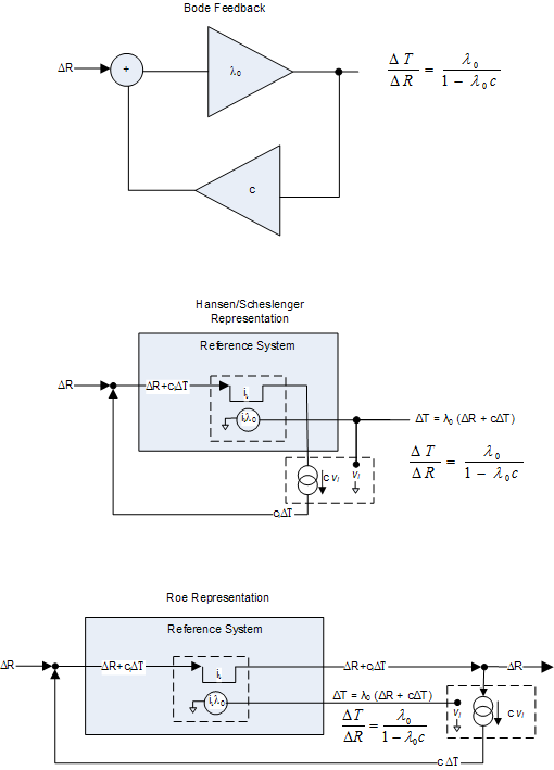
You’ve managed to filibuster long enough such that I doubt anyone is still paying attention but on the off chance that someone comes across this and wonders whose right, trust me I am, as any EE worth the title would have seen long ago.
Jeff,
Gerard Roe replied and here was his answer:
Hi George-
Ah, yes, there is an annoying typo in the figures. I’ve long been irritated by that aberration: it got inserted when the publishers reworked the figures and I failed to notice it in the proofs they sent me. Schematically, the correct output, as the equations of course reflect, is Delta T.
Best wishes,
Gerard
Jeff,
Your picture that shows the correspondence between Bode and the climate as outlined by Hansen and Schlesinger is what is claimed, however; it’s only meaningful when lambda0 and c1 are dimensionless constants and the output is expressed in the same units as the input. The other pictures have an internal source of power (the current source) that’s not the input stimulus and the climate system lacks that element.
Your representation of Roe is wrong based on his reply to my question about the typo in his paper.
As one EE to another, please examine this more carefully. The bottom line is that Roe’s lambda0 and Schlesinger’s Go are not representative of the open loop gain. The arbitrary assignment quantifying ‘f’ as a function of Go is incorrectly claimed to be what Bode calls the feedback factor which is the open loop gain, mu, times the fraction of output returned to the input, beta. Since Go and lambda0 are not the open loop gin and F or c1 is not the feedback fraction, the association with Bode’s beta*mu is invalid.
You should also pay special attention to the fact that the unacknowledged assumption of unit open loop gain is why Schlesinger assumed that gain could have arbitrary dimensions. He considered the closed loop gain (which he and Roe calls the system gain) the ratio of gains, rather than the ratio of output to input and in their formulation, what is claimed to be the open loop gain cancels. Clearly, the closed loop gain must be a function of the open loop gain, moreover; when you divide the closed loop gain by the open loop gain and assume the open loop gain to be 1, the result is the closed loop gain. Their formulation of the closed loop gain is only relevant when the open loop gain is assumed to be 1!
“Your picture that shows the correspondence between Bode and the climate as outlined by Hansen and Schlesinger is what is claimed, however; it’s only meaningful when lambda0 and c1 are dimensionless constants and the output is expressed in the same units as the input.”
That’s ridiculous. Trans-impedance amplifiers, a venturi, a hydraulic valve and heat pumps are are examples of transfer functions whose input units do not match there output units and which can be modeled in a feedback system perfectly well.
The other pictures have an internal source of power (the current source) that’s not the input stimulus and the climate system lacks that element.
“The other pictures have an internal source of power (the current source) that’s not the input stimulus and the climate system lacks that element.”
They are all equivalent!! They’re just different way of expressing the same mathematical relationship schematically. And neither controlled source requires internal power. They do no work. The ICVS drives an open and the VCIS simply circulates input flux back to the flux summing junction.
“Your representation of Roe is wrong based on his reply to my question about the typo in his paper.”
Then the middle diagram applies. The bottom diagram is not wrong in that it is shown to equivalent. it’s just a different way of looking at the same thing.
“Trans-impedance amplifiers”
As I explained earlier, the more general case requires inputs and outputs to be linearly related to each other such that superposition applies. Voltage and current are interchangeable metrics linearly related to each other through Ohms law and for a trans-impedance amplifier whose input is 1 ma and the output is 1V, the output would be 100V for an input of 100 ma. Bipolar transistors are current gain devices and not voltage gain devices, but in amplifier design, we almost always represent gain as a voltage gain. The kinds of electro-mechanical feedback systems you cited are not examples of amplifiers, but are more generalized feedback control systems that the basic Bode feedback amplifier model doesn’t trivially apply to.
In the climate model, the deltaR input and the deltaT output are not linearly related to each other. Starting at 0K, the first W/m^2 increases the surface temperature to about 65K, the next W/m^2 increases the surface temperature by only 11K more, and so on and so forth until the 239’th W/m^2, after all feedback has been accounted for, only increases the surface temperature by about 0.3C. Does this look linear to you?
“The ICVS drives an open and the VCIS simply circulates input flux back to the flux summing junction”
No. You are assuming an infinite input impedance, Joules of feedback are what gets fed back to the input and the current source in your diagram must produce those joules. The voltage source is assuming that the system is like a MOSFET with a virtually infinite input impedance, which is non representative of the climate in any way. You also realize that if you are modelling a MOSFET, there is no gain when configured as a pass device and the output voltage will always be less than the input voltage.
“As I explained earlier, the more general case requires inputs and outputs to be linearly related to each other such that superposition applies. ”
The plot below shows the error in estimating the 2xCO2 climate sensitivity incurred by linearizing lambda-zero. As you can see, it’s mouse nuts. The assumption of linearity of the temperature scales we’re taking about are perfectly valid.
“In the climate model, the deltaR input and the deltaT output are not linearly related to each other. Starting at 0K, the first W/m^2 increases the surface temperature to about 65K, the next W/m^2 increases the surface temperature by only 11K more, and so on and so forth until the 239’th W/m^2, after all feedback has been accounted for, only increases the surface temperature by about 0.3C. Does this look linear to you?”
What are you talking about? Without feedback the the first W/m^2 increases temperature by .266 K, the next gives .535K, the next .803K and at 4 W/m^2, 1.07 K. And yes that looks very linear to me (also see the plot above). Adding feedback simply amplifies/attenuates those values so that case is linear as well. I think you still don’t understand the very basics of these models which are linearized about some operating temperature. The models then give deltas from that point using deltaR = 3.7 W/m^2 for 2xCo2
” but in amplifier design, we almost always represent gain as a voltage gain. The kinds of electro-mechanical feedback systems you cited are not examples of amplifiers, but are more generalized feedback control systems that the basic Bode feedback amplifier model doesn’t trivially apply to.”
You must be terrified to get on an airplane since every surface control system is a feedback loop designed with basic Bode analysis. Again, just because Bode used amplifiers and just because his loop happened to be voltage to voltage doesn’t in any way restrict the analysis to those cases. The algebra doesn’t know whether your analyzing a mechanical system or an electrical system or an electro-mechanical system or a climate system. The only restriction is that the open-loop gain (defined as the gain seen with the feedback connection of the adder disconnected from input to the now disconnected output) be unitless so that at the adder you are adding like units. There is no restriction on the units of the individual gain blocks as long as there _product_ is unitless.
Last night my grandson came to visit. Ten years ago he was 22 inches long. He has “gained” nearly 4 ft in height. He doesn’t have an external power source, every blessed inch was fueled by the sun.
But if your grandchild didn’t eat, that growth would not have happened. People have no internal power supply, otherwise you would not need to eat, nor is your grandchild a linear active amplifier as described by Bode’s gain equation, so what’s your point?
The basic flaws in your understanding seems to be over generalization and a failure to recognize that a system must adhere to the simplifying assumptions predicating an analysis before that analysis becomes relevant. You also don’t seem to understand the difference between linear amplifiers that employ feedback and a feedback control system. The thermostat in your house is a feedback control system, but does not exhibit active gain and is not an amplifier. Bode’s analysis is specific to linear amplifiers providing power gain. The climate system is more like a feedback control system than a feedback amplifier and definitely does not exhibit power gain.
All 500+ pages in Bode’s book are exclusively targeted to the design and analysis of linear amplifiers employing feedback, as is clear from the title of his book. While feedback control systems, like an autopilot or a thermostatic control system may contain linear amplifiers as components, the end to end behavior of such a system is not described by Bode’s gain equation.
“But if your grandchild didn’t eat, that growth would not have happened.”
All natural sources of energy on earth including food are stores energy received from the sun. Your premise seems to be that gain is not possible without an external power source. There are many counter examples.
” You also don’t seem to understand the difference between linear amplifiers that employ feedback and a feedback control system. The thermostat in your house is a feedback control system, but does not exhibit active gain and is not an amplifier. Bode’s analysis is specific to linear amplifiers providing power gain. ”
If you don’t think thermostatic control (or any servo-loop for that matter) is amenable to Bode analysis you’re flat wrong. I’ve designed many phase-lock loops in my 30+ years. A PLL contains a phase detector which converts a time-difference to a voltage, an integrator to provide low frequency gain, a voltage-controlled oscillator which takes and input voltage and converts it to a frequency, another pure integrator which converts frequency to phase and a divider to complete the loop by converting phase to a time-difference. None of these blocks conform your ridiculous restrictions. None of them are amplifies, none of them have the same output units as inputs, almost all of them are non-linear yet Bode analysis predicts perfectly their dynamic responses to perturbations, their stability margins, their noise suppression characteristics and settling times.
Your continual spouting of misleading nonsense is a disservice to the readers here who don’t know how far over your head this entire subject remains.
Here’s an example of an illustrative passive system with gain (passive in the sense that the only power source is the pump, analogous of the sun). The pump is assumed to have virtually infinite HP such that it provides constant flow rate R regardless of loading effects. A portion (alpha) of the output stream is fed back to the reference system through a venturi. The system output variable is taken to be the velocity of the stream through the reference system. As alpha approaches 1, the venturi effect is longer longer applicable but over some range of alpha, the velocity through the reference system is seen to increase, i.e. the system exhibits gain for the chosen system variable.
“The system output variable is taken to be the velocity of the stream through the reference system”
My point stands regarding your fluid dynamic example. The system produces no power gain. If you put a powered impeller in the system, then it becomes active in the Bode sense. In Bode’s derivation of the stability criteria he shows how the additional energy from the implicit power supply (power gain) is what introduces the positive real component in the poles and which can result in potential instabilities. This is why he can infer that passive systems, per his definition of having no internal source of power, are unconditionally stable.
Regarding PLL’s and DLL’s, I’ve designed, implemented, characterized and put into production many such circuits as both discrete and integrated implementations and while Bode’s stability analysis certainly applies since identifying poles and zeros can be done for any arbitrary nodal network, the linear amplifier model he uses as an example of the simplest feedback loop that his analysis can apply to is definitely not representative of a PLL or DLL. While its not uncommon for a PLL to contain a linear amplifier as a component and of course a feedback circuit implementing a voltage controlled oscillator is another, nested feedback systems like this are not representable as a single, equivalent feedback circuit, unless they are all passive (no internal sources of power) since otherwise, there’s the possibility of multiple poles with different real components.
You still haven’t been able to internalize the difference between the stimulus that’s explicitly accounted for by the basic amplifier model and Bode’s implied infinite capacity, internal power supply that provides the power behind the gain. Sure, you can extend the model to account for all sorts of limitations, but this was not done as Bode was applied to the climate. Instead, the simple model was inappropriately applied to a system in a way that doesn’t conform to the simplifying assumptions he sets out.
Nick Stokes said “But I do think the output in Fig 2 would be more logically labelled ΔT. In fact, his text says that:“In general terms, the reference system takes a perturbation in the forcing, R_f , and converts it into a response, T₀ (Figure 2a).”
After closer inspection Roe’s formulation is correct. The drawing is misleading because normally a label above a block is meant to infer the gain of that block. In Roe’s diagram this is not the case as can be easily seen if you go through his derivation. Roe’s reference system is a Kirchhoff node that has equal flux density as both it’s input and output. I’ve depicted his formulation schematically below.
Note in particular that the temperature output is a sensible by-product of the flux flowing through the reference system. I rather like this formulation because it affords the potential for correcting one of the short-comings of these simple models which tens to be spatially inconsistent. What I mean is that radiative balance (depict by the summing nodes) takes place at the TOA but in reality at the TOA the temperature is held fixed, it’s the emission altitude that changes. Hence the feedback pick-off point cannot be at the TOA because at that point there’s no ΔT to force the feedback. I haven’t quite worked out the details yet but this could be rectified by the addition of a regulatory loop modeling the lapse rate feedback that holds the TOA ΔT constant and has the surface ΔTs as the sensible output and the feedback pick-off point. I could never quite see how to add this to the voltage analogous form of Hansen and others but it looks straight forward with Roe’s “current node” formulation.
In any case, the top post is hopelessly muddled and has only made a topic which baffles many more, not less, confusing. Argh.
Accidentally linked an older and incorrect version. Here’s the correct one. Sorry for the confusion
Treating the earth as a blackbody radiator for the purposes of theorizing is the geological equivalent of the ‘spherical cow’ https://en.wikipedia.org/wiki/Spherical_cow
and the alleged feedback mechanisms are the equivalent of the ‘assumed can opener’ https://en.wikipedia.org/wiki/Assume_a_can_opener
In a chaotic system feedbacks may be positive, negative, or neutral depending on variable of which we are taking no account.
tadchem,
Perhaps, a better understanding of equivalent modelling is in order.
http://www2.gsu.edu/~mkteer/equival.html
George
Good grief.
Fill an enclosed room with CO2 – 1,000,000 ppm! Apply formulae, feedbacks, models, magical incantations.
The temperature changes not at all.
CO2 warms nothing. The act of producing CO2 generates heat. Heat warms stuff – thermometers included.
Temperatures change from day to night, winter to summer. CO2 concentrations have no measurable effect at all. Complete and utter nonsense. Cargo cult Scientism, swallowed whole by the stupid and the gullible. What fun!
Cheers.
Looking at the price of my energy bill, the tax that I pay on petrol, the tax that I pay for flying, I would not describe it as fun.
Every thing that you buy has had its price hiked by this obsession.
It would really liberate the economy if all these taxes, subsidies, expenses were abolished. It acts like a straight jacket and is producing a poorer world for our descendants.
Sheesh. Not this nonsense again. CO2 doesn’t produce energy, it blocks the transmission of energy.
Correct. The energy input is solar. AGW is about slowing the rate of cooling. The whole violation of COE argument is a gross mistatement/misunderstanding of the basic GHE mechanism. And it gets worse. There is no doubt that water vapor warms via GHE and that clouds cool bia albedo and at Earths absolute global temperature configuration maintained by solar imput and WVF, the system is stable and damped (via cloud albedo). The WVF question is whether it warms more with more CO2 (( almost certainly yes) and if so by how much (observational EBM says by about half of what climate models say). The cloud feedback question is whether they cool more or less with more CO2, and by how much. All the lesser feedbacks roughly cancel to zero.
MarkW September 8, 2016 at 8:20 am
Temporarily. In the end the “blocked” energy leaves the building just like “Elvis”
michael
Mike; True, but the longer it takes to leave, the warmer the planet gets. Since the incoming energy is constant.
“True, but the longer it takes to leave, the warmer the planet gets. Since the incoming energy is constant.”
Why do you think that adding CO2 to the atmosphere appreciably slows the rate at which radiation escapes the atmosphere into space? Since the atmosphere is mostly composed of non-greenhouse gasses that don’t radiate IR, adding CO2 makes it both a more efficient absorber and a more efficient radiator. And it doesn’t need to absorb any more radiation from the surface before it starts radiating away the heat capacity already within the the air around it that it picks up through kinetic interactions. The air should be able to radiate away the same amount of heat at a lower temperature.
How can adding CO2 to the atmosphere both raise amount of heat stored in the land and oceans (surface temperature goes up) AND raise the amount of heat stored in the atmosphere (air temperature goes up) by becoming better at radiating away the heat it indirectly absorbs from a fixed solar input? I can see this to the extent that the CO2 is absorbing heat radiated from the Earth that would otherwise escape directly to space without being absorbed at all by the atmosphere, since the air is less efficient at radiating to space than the surface. But I’m far less persuaded by the argument that adding CO2 can still raise air and surface temperatures even after all the IR emitted from the surface is already absorbed by the atmosphere via the lapse rate.
“Why do you think that adding CO2 to the atmosphere appreciably slows the rate at which radiation escapes the atmosphere into space?”
It doesn’t slow the radiation flux, it impedes it. A resistor doesn’t slow the current passing through, but it increases the voltage.
A point often overlooked is that any feedbacks which exist, operate with temperature as the input, and temperature as the output. CO2 is not in any way involved in the feed back loop. Thus, ANY temperature increase would trigger the feedback, not just a CO2-induced warming.
That being the case, it’d kind a hard to see how these feedbacks can act in the way the alarmists predict, since if they did, any historical warm phase would have resulted int the climate going out of control. CO2 or no CO2, the result would have been the same, runaway warming.
The other observation is that ice age cycles look a bit like the kind of waveform you get from a relaxation oscillator. In this kind of (electronic) feedback arrangement, a small injection of current triggers a strong positive feedback and a rapid rise of current, until a limit is reached. The feedback then ceases and the current falls back to zero -gradually, if there is an inductor in the circuit.
If the ice age cycles are indeed due to such a mechanism, then the trigger point is at the coldest phase, which we are presently well away from. Therefore claims that we are at a ‘tipping point’ for rapid warming seem unlikely. It is more likely that we are around the point where the feedback hits the limit and temperatures start to gradually fall.
One reasonably good argument for limiting CO2 emissions is that we’re in relatively uncharted terrain: What if high CO2 levels “change the rules” and makes the current state similar to the glaciation state, where a small perturbation can cause a sudden jump to a different stable state with much higher global temperatures? I do not think so myself (I think it’s unlikely that the current ocean configuration, with e.g. the isthmus of Panama closed, is compatible with a state with much warmer oceans, and that CO2 does little to change this), but I still think this is a reasonable argument for precaution.
We are in uncharted territory regarding CO2 only if history started a few hundred years ago.
In the past few decades we’ve gone from CO2 concentrations of around 280ppm to just over 400ppm.
However in the past, CO2 levels were well over 5000ppm and could have been as high as 7000ppm.
There is nothing unusual or “uncharted” about current CO2 levels.
No inductor, but you can do the same with a capacitor, and there are a couple of those to work with. The oceans are long term storage, and the atmosphere is a short term storage.
Inductors are like mass. That is once something starts moving it wants to keep moving.
Perhaps air and water currents could be like inductors. Very small ones though.
@ur momisugly MarkW
September 8, 2016 at 8:20 am: Absorbers (so-called ‘blockers’) must emit. Though collision takes it away orders of magnitude faster….
Ian,
It’s certainly true that ice albedo enhances ice ages, but at the depths of an ice age, 1/2 or more of the planet’s surface is covered by ice. The current yearly average ice is about 12-13% and it’s hard to get much lower since winter interferes. The planet is pretty much out of dynamic range for ice feedback to enhance warming any more than it already does, however; there’s a lot of head room to go in the other direction as evidenced by ice ages. So the effect is one of albedo variability which is not really considered of part of the feedback model which is mostly concerned with the path from surface temperature to output emissions.
A parallel path from solar input to the surface is modulated by albedo, but for the purposes of small perturbations of GHG related ‘feedback’, albedo is considered constant. If you consider the Earth a capacitor, there are independent resistors to charge (solar) and discharge (LWIR) where the discharge resistance is smaller.
If you examine the effective sensitivity along the input path (plot plot albedo input vs. surface temperature), its closer to that of an ideal BB at the surface temperature. That the output path sensitivity is larger than the input path sensitivity means that the output path reacts faster to change than the input path which is why the output path sets the upper bound on the sensitivity at a little more than 0.3 C per W/m^2 while the input path sets the lower bound of a little less than 0.2C per W/m^2 and nowhere near the 0.4-1.2C per W/m^2 claimed by the IPCC.
The Antarctic has an average temp many 10’s of degrees C below 0 and where even the daytime summer highs never exceeds 0C across much of the continent. The ice survived the last interglacial when the average temps are estimated to be as much as 3C warmer than today for thousands of consecutive years. Being at a high altitude does make a big difference. You can find snow at those altitudes even at the equator. I was skiing on snow left over from last winter at an even lower altitude in the Sierra Nevada mountains just last weekend. BTW, as compared to previous years, the snow pack has been melting significantly slower than usual.
The ice cores also tell us that the thickness of ice in warm years is more than in cold years, so during the warmer periods, the ice builds faster as it also melts faster all on a seasonal cycle, but leaves a net increase that is larger than during colder periods.
It would take millions of years of continental drift or a large impact event in Antarctica to even start and make a dent in the Antarctic ice pack and the ice in Greenland is much the same way, so concerns about rising sea levels and massive ice melt caused by CO2 are wildly overblown.