By Christopher Monckton of Brenchley
Judge Alsup, in the California global warming trial, has accepted the amicus curiae brief from my eight distinguished colleagues and me. The brief now becomes an official part of the court documents. The judge may yet ask all parties to respond to it.
The initial reaction of the two California cities that brought the case against five oil companies, demanding that they should fork out billions to fend off sea-level rise, was to use the traditional totalitarian tactic of attacking our personal reputations. So much easier, that, than producing a scientific argument. The judge was unmoved.

A simple feedback amplifier circuit from Bode (1945, page 31). Note that the input and output signals are not deltas but entire values. Numerous climate papers cite the feedback math in Bode as the basis for climate feedback analysis.
Meanwhile, my account here at WUWT of the grave error that we have discovered right at the heart of climate physics has attracted 1000+ comments – not unprecedented, but rare. The high level of activity shows that the climate fanatics are worried – very worried.
But not worried enough to work out a credible line of attack. I have seldom seen so many feeble arguments in one place. On countless occasions, those who so often try to disrupt comment threads here with a melange of spiteful ad-hom attacks and half-baked pseudo-science (one of them even sent me a vile email offering gratuitous and profoundly offensive medical advice, though he was not a medic, a sure sign of extreme desperation on his part) found themselves attacking official climate science.
To these I felt like replying: “Comrade, do you realize you are criticizing the Party Line? Do you not know the penalty for that?” Instead, I suggested they should address their concerns to the climate clique, not to me.
Official climatology’s error is grave. It has hitherto been assumed that, while a change in temperature, such as the small warming from adding the non-condensing greenhouse gases to the atmosphere, can induce a feedback response, the Earth’s far larger emission temperature somehow cannot.
The most significant objection to our argument came from Roy Spencer, who said official climatology defines a temperature feedback as an extra forcing induced by a change in temperature, but not by the original temperature itself.
That is indeed the definition. But merely because official climatology says white is black, we should not be too hasty in bidding farewell to white.
With respect, the question is not whether official climatology defines feedbacks in such a way as to exclude from the account the large feedback response to the Earth’s emission temperature, but whether in reality the emission temperature actually induces that large feedback response.
When I was in Moscow recently, presenting our result to members of the Russian Academy of Sciences, Professor Mojib Latif, an IPCC lead author, recommended a paper by several NASA authors, Lacis et al. (2010), who had run a general-circulation model in which they had removed all non-condensing greenhouse gases from the atmosphere and had studied how the climate would evolve over 50 years.
Their conclusion was that after 50 years with no greenhouse gases the Earth’s albedo would have risen from today’s 0.293 to 0.418, and that mean surface temperature would have fallen from 288 K to 252 K, a drop of 36 K, of which 9 K, they imagined, was the loss of directly-forced warming from the non-condensing greenhouse gases and the remaining 27 K was the loss of feedback response to that directly-forced warming.
What would the emission temperature be if the albedo were 0.418? The answer, assuming today’s insolation, is 243.3 K. Yet Lacis et al. said the equilibrium temperature with no non-condensing greenhouse gases would be 8.7 K higher than that, at 252 K. That is manifestly a feedback response to emission temperature, albeit an unrealistically low one.
Since we shall want to compare the pre-industrial and industrial-era values of the feedback fraction f, we shall take the 287.5 K surface temperature in 1850 as the equilibrium temperature for the pre-industrial calculation. And, when we come to the industrial-era calculation, we shall bend the argument rather too far in favor of official climatology.
Lacis says one-quarter of the [35.5 K] difference between 252 K and [287.5 K] [i.e. 8.9 K] is directly-forced warming from the non-condensing greenhouse gases, while three-quarters of the [35.5] K [i.e. 26.6 K] is the feedback response to that [8.9 K] of greenhouse-gas direct warming. Thus, Lacis takes the feedback fraction f to be three-quarters, or 0.75.
Then the 44.2 K difference between emission and 1850 temperatures comprises 8.7 K feedback response to emission temperature; 8.9 K directly-forced greenhouse warming; and 26.6 K feedback response to direct greenhouse warming.
According to our corrected method, f is a lot less: 1 – (243.3 + 8.9) / 287.5, or 0.123. In that event, the 44.2 K comprises 243.3 f / (1 – f) = 34.0 K feedback response to emission temperature; 8.9 K directly-forced greenhouse warming; and 8.9 f / (1 – f) = 1.3 K feedback response to direct greenhouse warming. That seems a more reasonable apportionment.
Now for the industrial-era value of the feedback fraction. Lacis says that for “the entire terrestrial greenhouse effect” and also for “current climate” the feedback fraction is 0.75. Not much nonlinearity there, then. But many commenters worry about nonlinearities, so we shall go overboard to accommodate them.
For our corrected method, we begin by noting that from 1850-2011 the IPCC’s estimate of total net anthropogenic forcing was 2.29 Watts per square meter; that the Planck parameter is 0.313 Kelvin per Watt per square meter; and that, therefore, anthropogenic reference warming before accounting for feedback was 2.29 x 0.313 = 0.72 K. Yet, since 0.76 K warming was observed over that period, our industrial-era feedback fraction, to first approximation, is 1 – 0.72 / 0.76 = 0.05.
However, commenters have asserted that the equilibrium warming will be perhaps 40% greater than the 0.76 shown in the temperature record, because some of the warming will have gone into the ocean, and may return to warm the atmosphere in a few decades.
In that event, our industrial-era feedback fraction becomes 1 – 0.72 / (0.76 x 1.4) = 0.32, or more than two and a half times the pre-industrial feedback fraction. That should handsomely allow for the nonlinearities in feedbacks whose omission from the original calculation several commenters complained of. In reality, the nonlinearity will be far less than this.
Armed with the probably much inflated industrial-era feedback fraction 0.32, we can derive Charney sensitivity (equilibrium sensitivity to doubled CO2 concentration) by noting that the CMIP5 estimate of the CO2 radiative forcing is 3.5 Watts per square meter, which, when multiplied by the Planck parameter 0.313 Kelvin per Watt per square meter, gives reference warming 1.1 K. Charney sensitivity is then 1.1 / (1 – 0.32) = 1.6 K, and not the 3.3 K that is the CMIP5 models’ current mid-range estimate.
Now for some questions which, in our submission, anyone who wishes to adhere to official climatology’s notion that emission temperature induces no feedback response must credibly answer.
Question 1: If, from Lacis’ model, the 8.7 K difference between emission temperature 243.3 K and equilibrium temperature 252 K with no non-condensing greenhouse gases is not a feedback response to emission temperature, then what on Earth is it?
Question 2: How is it that emission temperature of 243.3 K induces a feedback response of only 8.7 K (or 0 K if, notwithstanding Lacis’ result, you think emission temperature cannot induce any feedback response at all), and yet that the 27-times-smaller 8.9 K direct warming from the presence of the naturally-occurring, non-condensing greenhouse gases induces as much as a 26.6 K feedback response?
Question 3: Would it not be more likely that, as we find, the feedback response to emission temperature of 243.3 K is 34.0 K, while the feedback response to directly-forced greenhouse warming of 8.9 K is only 1.3 K, rather than Lacis’ 8.7 K and 26.6 K respectively?
Question 4: Since feedbacks are denominated in Watts per square meter of the temperature that induces them, how do the feedbacks know that they should not respond at all to the emission temperature of 243.3 K but that they should suddenly respond very strongly by quadrupling the 8.9 K directly-forced reference warming from the non-condensing greenhouse gases?
We have here made the most generous allowance for the points raised by commenters, and yet Charney sensitivity, at 1.6 K, is not a lot greater than the 1.2 K in the original article.
In my submission, then, there will simply not be enough global warming to require any mitigation measures at all. If we are right, this really is game over.
All this talk of pre-industrial has to small problems, firstly there is no real agreement on what date this would be, an secondly the idea that we ‘known ‘ climate or weather factors from these early dates is ‘problematic’ to say the least
In reality all dates which are picked for pre-industrial will give you a system that in no way matches what we have to day , virtual no ocean coverage , vast areas of land such has Africa and the Middle East and South America with little of nothing nothing , and other others of land such as Europe with limited measurements with no where near the degree of accuracy or regulations over data collection and management required for these values to be consider good to the level now being claimed for them .
Hence the need to use ‘proxies’ such has magic trees in the first place .
We do not ‘known ‘ these values in the way we now think of knowledge, we can ‘guess ‘ them but we are not even sure what factors may effect those guesses. So the comparison between current knowledge and past knowledge that gives us the degree of change of any type consider, is significantly affected by what the actual state of past knowledge is. And on this front the situation is far from clear .
In response to KNR, the beauty of focusing on the Lacis experiment is that it covers the period 1800-1850, when conditions were close enough to the present to allow some reasonable conclusions to be drawn.
A common misconception about climate feedbacks is that CO2 is the input and temperature the output. NOT SO. The inputs and outputs to the feedbacks are both temperature.
Now, experience from other disciplines, especially electronics, tells us that you cannot have a positive feedback loop with gain, in which the output is directly connected to the input, Such an arrangement would be completely unstable. There would be no need for CO2. The climate would already be unstable, from the word go.
Since that is not the case, we can assume that such feedbacks do not exist.
You can of course have a negative feedback loop in which the output and input are connected, without that leading to instability. Which suggests that if feedbacks do exist in the climate system, they are negative feedbacks..
Agreed. If the feedback response to CO2 forcing was net positive humanity wouldn’t be here to argue about it.
Surely you mean net greater than 1, not net positive! http://electronotes.netfirms.com/EN219.pdf
Of course both are temperature. But the argument from the AGW crowd was: CO2 increase –> Temp increase –> H20 vapor increase –> more Temp increase. So that feedback was argued to be via temperature. With the influence from CO2 at half or less than half of that from water vapor. Say if CO2 caused +1 C than H2O would cause an additional +2.
If it is not possible that there is this feedback via temperature, then the water vapor influence must be autonomous.
We have had a doubling of the population on Earth since 1950, that means more food, which requires more agriculture (including rice paddies) and more irrigation. It is argued that this doesn’t have any effect, but that seems rather odd.
Their claim is that H2O has a shorter life-cycle in the atmosphere. But what really matters is the yearly balance of additional production versus consumption of whatever GHG is put into the atmosphere, including water. And as long as we keep on pumping more water into the atmosphere than before 1950, assuming the ‘ consumption’ (increase in rain etc) is not keeping up, then the average amount should now be higher than before.
False –
A positive feedback can approach f=+1 as closely as you dare, and is still sable. It is singular at f=1.
http://electronotes.netfirms.com/EN219.pdf
“offering gratuitous and profoundly offensive medical advice, though he was not a medic”
Hugely amusing way of putting it!
Once you admit to the mere possibility that they’re all lying and have done so from the outset, EVERYTHING else falls into place. The climate has always changed, there have always been weather events that adversely affect some human beings – but as my 14-year old sons says, nobody thought of a way to get rich and find new ways to exercise power over their fellow human beings from it until recently. But this BS is viral and is mandated by the irresistible power of the state, so it may also be unstoppable.
I saw my plea for more signatures on my petition to the Government of Canada (https://www.change.org/p/the-honourable-james-gordon-carr-minister-of-natural-resources-open-letter-to-the-government-of-canada-re-climate-change) go ignored, so have concluded, today being my 59th birthday and a good time for reflection, that I’m done fighting. When it gets to the point that scientific illiterates like the mayors of a couple of Californian Podunks think they can fill civic coffers with money stolen from oil companies, well – f*ck it as a wise man once said. As far as governments and mainstream media are concerned, the truth has never mattered, not for one minute. Skeptics were consulted exactly once, and because the mandarins didn’t like what was said, never again (Senate hearings of angry IPCC authors and reviewers). Why would they be? We’re talking about TRILLIONS OF DOLLARS, folks! A hog trough without precedent and with no termination date. So good luck to you, especially Anthony, but as for me, after 20-odd years of being as involved as I know how, an extended period of ignoring it is well overdue.
@Nick Stokes March 27, 2018 at 9:45 pm
“Nick is under the impression that feedback doesn’t apply to DC.”
I said feedback can’t be generated by something that doesn’t change. You keep talking about DC that does change.
What a bizarre statement!!!
In DC opamps, ALL voltages fed into the input of the opamp are summed together.
Therefore the DC input value and the AC changing value are passed directly to the output after being multiplied by the gain.
There is nothing else involved in an opamp circuit.
You are wrong.
Now, just to give you something to bite on, what if the quiescent DC input voltage changed slightly?
Would it have an affect on the final output voltage?
Of course, all input voltages are summed together and multiplied by the gain an output.
Christopher Monckton is effectively saying the DC quiescent input changes slightly.
The DC quiescent input originates from the Sun and is influenced by atmospheric constituents.
But the output of the amplifier or anything else within the loop does not know or care about what changed in a feedback loop, they all have an effect.
Diagnosing faults in closed loop feedback circuits can be tricky. You have to open the loop and make some measurements.
A bit like in the head post.
“Therefore the DC input value and the AC changing value are passed directly to the output after being multiplied by the gain.
There is nothing else involved in an opamp circuit.”
People here are hung up on op amps. They are not the only amplifying device; they have internal circuitry that allows them to operate in differential mode. For a valve, junction transistor, FET etc you don’t get the output voltage by multiplying the input voltage by the gain.
“what if the quiescent DC input voltage changed slightly?”
There you go again. Gain and feedback operate on changes.
If Society Can’t Trust Science, What Can They Trust? Climate Sophist is Playing San Francisco Judge as a Complete Fool
https://co2islife.wordpress.com/2018/03/25/climate-alarmist-is-playing-san-francisco-judge-as-a-complete-fool/
” I have seldom seen so many feeble arguments in one place. On countless occasions, those who so often try to disrupt comment threads here with a melange of spiteful ad-hom attacks and half-baked pseudo-science (one of them even sent me a vile email offering gratuitous and profoundly offensive medical advice, though he was not a medic, a sure sign of extreme desperation on his part) found themselves attacking official climate science.”
Here is a rebuttal to Dr Allen’s presentation. It is really embarrassing how shotty their work is. They really must think this judge is a gullible fool.
Climate Sophistry In San Francisco; Half-Truths are Twice the Lie
https://co2islife.wordpress.com/2018/03/24/sophistry-in-san-francisco-half-truths-are-twice-the-lie/
Please, fellow skeptics, tell me you aren’t that gullible. This is embarrassing.
Of course feedback is an emergent feature of the climate models. If the models’ equations dictate that a quantity (such as temperature) that responds to a stimulus (such as net irradiation) itself causes more of that stimulus, then, broadly speaking, they implement feedback.
But do you really believe climate modelers think that things like water vapor, albedo, and clouds depend on temperature at 288 K but don’t at 255 K? Do you really think that Lord Monckton can reliably infer from simplistic linear arithmetic applied to the results of a single paper that climate modelers harbor such a fantastic notion? Do you really think he can so simplistically infer much about marginal values at 59°F in a water world from those at -1°F?
This is what Roy Spencer said:
I have no faith in those who believe they can predict future climate by programming supercomputers. But it strains credulity that they made the error Lord Monkton claims they did.
Let’s hope the trier of fact concentrates on Happer, Koonin, and Lindzen and doesn’t take the quality of Lord Monckton’s reasoning as representative of skeptic thought generally.
Unfortunately Roy doesn’t accept any thermal effect from descending air despite the well known phenomenon of adiabatic warming in descent and does not accept that at any given moment half the atmosphere has a rising component to its flow and half has a descending component.
Thus he falsely believes that convective overturning has a net cooling effect on the surface rather than a net zero effect (once the atmosphere is in place). Convection only had a surface cooling effect during the first convective overturning cycle during the formation of the atmosphere and since then the energy taken from the surface has been returning to the surface in a constant cycle.
His error in giving a net cooling effect to ongoing convective overturning means that he must counter that error just as alarmists do by proposing an equal heating of the surface by radiation downwards from GHGs.
In reality downward radiation has no thermal effect at the surface because its thermal effect is subsumed into the increasing efficiency of conduction as density increases during the descent along the lapse rate slope.
That conduction then feeds into ongoing convection which neutralises any surface warming effect from downward radiation.
Sadly, Christopher hasn’t realised that yet either.
It’s also possible you could just be wrong.
I know you think that Anthony, so thanks for letting me continue to contribute.
In fact I know I am right, that it is being picked up by increasing numbers of commenters and accords with basic non radiative thermodynamics.
Would anyone like to specify, simply, why it is wrong ?
I think some definitions are needed to understand Dr Spencer. Convection includes water vapor, which transports heat to above most of the CO2. Thus convection is cooling. I would consider conduction to be a minor component of cooling, as compared to evaporation. Without water on earth, there would be much larger temperature swings and daily high winds.
The average temperature data we collect is not sufficient to determine daily, hourly, heat transport over 100’s of years. Even a satellite, which traverses withing an hour, cannot collect data on say thunderstorms dumping heat 2 minutes earlier every day.(Willis)
sailboarder
You have to distinguish between condensing GHGs such as water vapour and non condensing GHGs such as CO2
For condensing GHGs they distort the lapse rate slope in ascent but then radiate to space from the condensate so that the descent is at the dry adiabatic lapse rate set by gravity. The radiation to space thus neutralises the lapse rate distortion in the ascent.
For non condensing GHGs they also distort the lapse rate slope in the ascent but that is not neutralised by radiation to space from a condensate so instead the distortion of the lapse rate slope in the ascent is neutralised by an equal and opposite lapse rate distortion in the descent.
Either way the effect on surface temperature for the system as a whole nets out to zero.
I explained it in detail here:
http://www.newclimatemodel.com/neutralising-radiative-imbalances-within-convecting-atmospheres/
Actually I think you misunderstand what he aims at. It is a bit like Jiujitsu or Judo, using mostly elements of your opponent to defeat him.
It reminds me of a regional Judo championship in NL when I was a very small and young boy. I was the youngest of our team I think. We had several official Japanese judges for some reason.
My (final) opponent was 2 ranks higher, several years older, much bigger and weighed about twice as much as me. He looked like a typical schoolyard bully. Clearly a hopeless task.
Shortly after the greeting I hooked him at the knee and pushed him slightly, he fell quite hard, flat on his back. His weight helped a lot…
Our Japanese judge grinned, waved his arms and hands in a move similar to calling a strike in baseball, and he yelled: Ippon !
🙂
Yes, I think that is right. For the purpose of this head post Christopher accepts the basic premise of a feedback and correctly points out that the alarmists appear to be referring to the feedback from extra CO2 provided by humans in isolation whereas if one considers the baseline feedback prior to human input then the human input is very small.
He also skips over the issue of whether it is really sun warmed oceans that might be increasing CO2 whilst our puny output is possible sequestered locally by enhanced vegetation growth.
However, if one denies that feedback issue altogether, as I think one should from the thermodynamics of a density related lapse rate, then the whole issue can be sidestepped and it would be nice if Christopher and others could begin to consider that side of things.
Basic thermodynamic principles relating to non-radiative phenomena are all one really needs to adequately explain the surface temperature enhancement above S-B of planets with atmospheres.
” But it strains credulity that they made the error Lord Monkton claims they did”
I don’t agree. Amplification and feedbacks can be modeled using electrical circuits. The climate system must be bounded by negative and positive feedbacks, otherwise we would have boiled off or frozen up by now. If MB has it right, the modellers need to explain their code. Why don’t they put explanations of their algorithms here for discussion?
Indeed they can. Such electrical circuits act in essence as analog computers. Analog computers have this in common with digital computers: garbage in, garbage out. We need to see the programming to determine whether what they’ve done is valid.
I’m inclined to believe that garbage has indeed gone into the climate models. To the extent that the modelers haven’t shown their work, moreover, I think they should. But sauce for the goose sauce for the gander. Despite being asked repeatedly by Bernie Hutchins about the specifics of his circuit–that is, about the programming of his analog computer–Lord Monckton has repeatedly declined to provide them.
Perhaps Monckton partisans calling for explanations of the modelers’ algorithms should consider the beam in their own eye.
Don’t whine. Wait for the paper.
Monckton of Brenchley March 28, 2018 at 8:49 pm
Don’t whine. Wait for the paper.
So stop whining that no-one has proposed a detailed critique of your work, since you haven’t published it yet and you won’t answer pertinent questions it’s impossible to assess it.
The irrational “Phil.” says I have complained that no one has made a detailed critique of our result. I have made no such complaint. Wait until the paper is published.
Mr Born would be credible if he were less petty.
Dear Monkton. Am a great admirer of your approach of lacing hard science with telling lay illustrations of it. The facts must win in the end, even if political idiots and their academic and renewable energy carpet baggers exploiting the pseudo science of catastrophic CO2 caused climate change use the proceeds to promote the lie that keeps on giving, by laws that claim reality is subservient to their statistical models, and even the proven laws of physics re energy. The second is easy to prove. ?dl=0
?dl=0
I believe I have a simpler, complementary response to the claims of disastrous global warming from CO2 emissions. It’s here, hope it helps someone:
I made the most telling one myself using a climate change site, wood for trees, from well respected data, Mauna Loa CO2 and corresponding Met Office global temperature set, plotted on the same linear axis with the base line suppressed. This needs comparing with the shameful deceit of selective time scales and over amplified temperature scale carefully selected from the noise in real Earthly climate change periodicities of significant change, as deployed to deceive by the pseudo climate scientist Brian “Poppy” Cox, and Piltdown Mann’s hockey stick, which used grossly manipulated dispararte historical data sets to create a bogus reality that denies the well recorded historic facts, etc., etc.
I suggest you don’t need no steenking models when you have the data in the graphs here.
Spot the disastrous correlation? Note lack of any tipping point as CO2 rises, partly because climate science KNOWS the already small CO2 effect/sensitivity rolls off logarithmically due to the band saturarion effect, Increasing negative feedback as CO2 levels rise. Wholly underwhelming.
As I feel it essential for serious science trained people outside the climate change cash flow to point out the nonsense of this supposedly correlated pair of variables at any significant level for humanity, I also rolled the others together. These are unadulterated (by me) well known data over various time scales of interest in the last interglacial. Obs or what? Nothing to see here in the way of significant correlation, CERTAINLY NO CONTROLLING EFFECT ON THE ATMOSPHERE DURING INDUSTRIALISATION TO BE SEEN. NOTHING TO JUSTIFY ATTEMPTS TO CONTROL THE ALREADY LOW LEVELS OF CO2 IN GLOBAL CLIMATE TERMS, ESSENTIAL TO PLANT AND ANIMAL LIFE ON EARTH.
POINT: It is self evident that creating models that use transfer functions to prove the opposite of measured reality is a very strange science to pursue, unless its to do with justifying the renewables racket and keeping the climate modellers grant cash flowing and egos inflated? Surely the point in all this is it is necessary for a cour to look behind the corporate veil of climate change to determine WHY such obvious nonsenses were and continue to be exaggerated? Who stands to gain. if not the planet or energy consumers?
Motive, opportunity, weapon. Trillions pa in easy Money, easy to manipulate politically green zealot alarmists, supposedly “super” computer models that can fortell the future by guessing the odds – promoted to a gullible public as an alternative reality to historical evidence.
Things that your ‘lible, to read in Mann’s bible, they ain’t necessarilly so.
The evil that men do lives after them……… etc.
If just one scientist somewhere can show the theory is wrong, then its wrong, doesn’ ‘t matter who made it. Except in climate science. Phlogiston and caloric come to mind….. Bad Science rules (BS)
Catt
Comment on myown above. I did the sensitivity figure defined above on the Mauno Loa 70 year record, its around 0.002 or 0.2%, assuming CO2 does all the change. Not very sensitive. Also negative or zero in earlier times within the current interglacial, pre and post industrialisation.
brianrlcatt March 28, 2018 at 10:23 am
Spot the disastrous correlation? Note lack of any tipping point as CO2 rises, partly because climate science KNOWS the already small CO2 effect/sensitivity rolls off logarithmically due to the band saturarion effect, Increasing negative feedback as CO2 levels rise. Wholly underwhelming.
Since you are aware that the response to CO2 is logarithmic I wonder why you insist on plotting it linearly?
I don’t insist, but I do prefer. You plot it how you like. Using a log scale for CO2 obviously compresses CO2 data and temperature would have to be the same, compressed, as the whole idea is comparable axes. Using a log scale thus defeats the object of comparing on a linear scale, e.g. maximising the demonstration of the insensitivity of temperature to CO2 . The numeric relationship is unchanged. Obs. This approach best dispays the lack sensitivity of global temperature to CO2 variation, the deceitful warmist graphs differentially amplify a much smaller range of the CO2 ppm to compare with the corresponding temperature range, and only show the time periods that exhibit positive correlation. So I remain unsure what your actual point is.
brianrlcatt March 29, 2018 at 12:26 pm
I don’t insist, but I do prefer. You plot it how you like. Using a log scale for CO2 obviously compresses CO2 data and temperature would have to be the same, compressed, as the whole idea is comparable axes. Using a log scale thus defeats the object of comparing on a linear scale, e.g. maximising the demonstration of the insensitivity of temperature to CO2 . The numeric relationship is unchanged. Obs. This approach best dispays the lack sensitivity of global temperature to CO2 variation, the deceitful warmist graphs differentially amplify a much smaller range of the CO2 ppm to compare with the corresponding temperature range, and only show the time periods that exhibit positive correlation. So I remain unsure what your actual point is.
That T has a logarithmic dependence on CO2 so the honest way to present it is log(CO2) vs T, ‘comparable axes’ as you put it, plotting linear CO2 is ‘deceitful’.
In case anyone wants to argue that the subjects in that article by Lacis et.al. is in some way not a standard part of climate science, then just take look at this course syllabus:
http://www.atmos.albany.edu/facstaff/brose/classes/ATM623_Spring2015/Notes/
And here is AE Dessler (arguing for ECS>2 °C).
See in video at 2:00: double CO2 -> Ts increase –> humidity increase –>[loop back to Ts increase for feedback]. He also notes that f stands for amplification from feedbacks at 2:13.
Sounds good.. but the data sets he uses are not global. One might conclude for example that the 1910 to 1940 temperature rise is a warning to us that maybe nothing special is happening. Here is what Phil Jones had to admit:
1860 – 1880 0.16 C 20 years of warming, followed by 30 years of cooling.
1910 – 1940 0.15 C 30 years of warming, followed by 40 years of cooling.
1975 – 1998 0.16 C 20 years of warming followed by nearly 20 years of next to no warming(the so called “hiatus”).
Trends : Phil Jones CRU in East Anglia, UK. (Head of UK climate research unit, which tabulated the world wide temperature history. For confirmation, Google his 2009 interview by the BBC where he confirms these data trends in the temperature record)
ENSO is the negative feedback, in response to solar variability, El Nino conditions regularly occur during periods of slower solar wind, and La Nina conditions during periods of faster solar wind. The exception being during volcanic aerosol events, where El Nino conditions typically dominate.
Here are some better estimates for ECS and TCR by Lewis & Curry, 2014.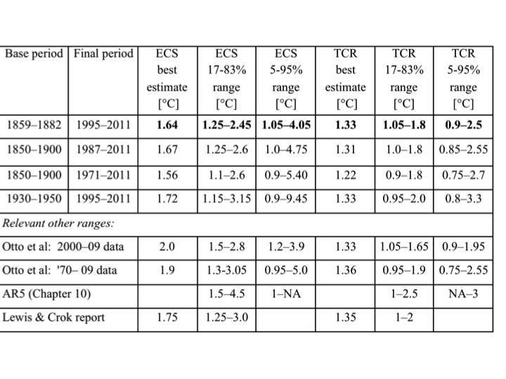
https://judithcurry.com/2014/09/24/lewis-and-curry-climate-sensitivity-uncertainty/
Table 1 gives the ECS and TCR estimates for the four base period – final period combinations used.
Full paper: https://niclewis.files.wordpress.com/2014/09/lewiscurry_ar5-energy-budget-climate-sensitivity_clim-dyn2014_accepted-reformatted-edited.pdf
So periods of stronger solar wind drive La Nina conditions, reducing atmospheric Water Vapour, and providing a strong negative feedback. Take it to the AMO scale, weaker solar wind since 1995 has driven a warm AMO, increasing water vapour in the lower to mid troposphere and reducing WV in the upper troposphere and lower stratosphere. Negative feedbacks all the way, less solar near infrared is absorbed at upper levels, and a greater WV greenhouse effect at mid-lower levels. The warm AMO even reduces CO2 uptake, another negative feedback.
sailboarder March 28, 2018 at 12:24 pm
Sounds good.. but the data sets he uses are not global. One might conclude for example that the 1910 to 1940 temperature rise is a warning to us that maybe nothing special is happening. Here is what Phil Jones had to admit:
1860 – 1880 0.16 C 20 years of warming, followed by 30 years of cooling.
1910 – 1940 0.15 C 30 years of warming, followed by 40 years of cooling.
1975 – 1998 0.16 C 20 years of warming followed by nearly 20 years of next to no warming(the so called “hiatus”).
Trends : Phil Jones CRU in East Anglia, UK. (Head of UK climate research unit, which tabulated the world wide temperature history. For confirmation, Google his 2009 interview by the BBC where he confirms these data trends in the temperature record)
That’s not what he ‘admitted’, here’s what he said in response to the question, (notice there’s no reference to the years of cooling you inserted):
“Temperature data for the period 1860-1880 are more uncertain, because of sparser coverage, than for later periods in the 20th Century. The 1860-1880 period is also only 21 years in length. As for the two periods 1910-40 and 1975-1998 the warming rates are not statistically significantly different (see numbers below).”
He was also asked:
“Do you agree that from 1995 to the present there has been no statistically-significant global warming”
To which he replied:
“Yes, but only just. I also calculated the trend for the period 1995 to 2009. This trend (0.12C per decade) is positive, but not significant at the 95% significance level. The positive trend is quite close to the significance level. Achieving statistical significance in scientific terms is much more likely for longer periods, and much less likely for shorter periods.”
Notice he didn’t say there was no warming as your post suggests, but that there was warming but there wasn’t enough data for it to be statistically significant at the 95% level.
In a follow-up interview the next year he pointed out that the extra year’s data allowed the trend to be statistically significant:
“Basically what’s changed is one more year [of data]. That period 1995-2009 was just 15 years – and because of the uncertainty in estimating trends over short periods, an extra year has made that trend significant at the 95% level which is the traditional threshold that statisticians have used for many years.”
“HadCRUT shows a warming 1995-2010 of 0.19C”
Assuming only atmospheric feedbacks account for Earth’s surface temperature overlooks the elephant in the room. What about the capacitors and diodes in the power supply? The largest ‘greenhouse effect’ that raises Earth’s average surface temperature is within the ocean rather than within the atmosphere. Oceans force surface heating during the night by convection, such that their surface barely cools.
The ocean is best understood as a heat sink, not a heat source (except to the extent that there is warming from below, particularly at the mid-ocean divergence boundaries).
The oceans as capacitor, yes that seems a reasonable comparison. They can store and release energy.
Also has a clear dampening effect, removes spikes, smooths the ‘current’.
Thermal reservoir:
“A thermal reservoir, a short-form of thermal energy reservoir, or thermal bath is a thermodynamic system with a heat capacity that is large enough that when it is in thermal contact with another system of interest or its environment, its temperature remains effectively constant.[1] It is an effectively infinite pool of thermal energy at a given, constant temperature. The temperature of the reservoir does not change when heat is added or extracted because of the infinite heat capacity. As it can act as a source and sink of heat, it is often also referred to as a heat reservoir or heat bath.
Lakes, oceans and rivers often serve as thermal reservoirs in geophysical processes, such as the weather. In atmospheric science, large air masses in the atmosphere often function as thermal reservoirs.”
https://en.wikipedia.org/wiki/Thermal_reservoir
Can act as a heat source, like at night when the upper ocean convects warmth to the surface.
Jaap wrote:
“Also has a clear dampening effect, removes spikes, smooths the ‘current’.”
Of the diurnal cycle, though big spikes are created by ENSO.
Christopher writes:
“(except to the extent that there is warming from below, particularly at the mid-ocean divergence boundaries)”
That is the ocean floor being the source and the ocean being the sink.
Magmatic intrusions warm the ocean, which passes some of the heat to the atmosphere. To this extent, the ocean is a source as far as the atmosphere is concerned.
The ocean surface is a source of heat every night regardless of the contribution by hydrothermal vent etc.
My question on all this is why didn’t the climate model peer reviewers do this or something similar years ago? I had to review complicated, iterative computer programs years ago in the nuclear industry and it was a requirement that an alternate means of verifying the computer results be performed to make sure the computer output made sense. You would usually do this by doing a simplified hand calculation, but sometmes it
took some creativity. That is exactly what Lord Monkton and friends did. If I was the judge I’d ask why did an outside group have to do it, and why didn’t the peer reviewers already do it? Maybe it was not a requirement here because it would be eventually validated with satellite monitoring (with billions spent in the interim) or maybe this is something engineers do (because lives are at stake) but scientists don’t, but whatever the reason it would have been good practice and most definitely financially prudent.
Dr. Roy Spencer peer reviewed “The Magic Temperature Feedback” by The Lord (Monckton) of the Rings”
http://www.drroyspencer.com/2018/03/climate-f-words/
http://i.myegy.to/images/679cdb58c95e.original.jpeg
The site that sells virtual calculaters
http://www.calqlata.com/
has a lot of science on it and one of their topics is on earth’s atmosphere. I quote from the site.
“Given that we know the density of air (ρₐᵢᵣ) at sea level is approximately 1292.8g/m³, the principal properties for each component gas at sea level are …
[units are evaluated to corroborate the formulas]:
The molecular density of air (ρᴹₐᵢᵣ) = ρₐᵢᵣ ÷ Σρᴹₓ.RAMₓ [g/m³ ÷ % x g/mole = mole/m³]
The molecular density of each gas (ρᴹₓ) = % . ρᴹₐᵢᵣ (mole/m³)
and the mass density of each gas (ρₓ) = ρᴹₓ . RAMₓ [mole/m³ x g/mole = g/m³]
Air pressure (pₐᵢᵣ) is 101325N/m²
Gas pressure (pₓ) = % . pₐᵢᵣ (N/m²)
Gas mass pressure (pmassₓ) = pₓ . (r+H)² ÷ G . m₁ [N/m² x m² ÷ N.m²/kg² x kg = kg/m²]
which is the mass of gas in the atmospheric column and ‘H’ is the altitude of its centre of mass
i.e. 50% of the mass lies above this altitude and 50% of the mass lies below it
To conclude for the principal gases in the earth’s atmosphere @ur momisugly 273.15K:
gas RAM percentage mole density mass density mass pressure
g/mole ≈% (ρᴹₓ) mole/m³ (ρₓ) g/m³ (pmassₓ) g/m²
N₂ 28.0134 78.087% 34.42594855 964.387867 8087362.21571
O₂ 31.9988 20.95% 9.236154828 295.5458711 2169233.80954
Ar 39.948 0.93% 0.410005918 16.37891643 96258.45023
CO₂ 44.095 0.03% 0.013225997 0.583200354 3104.60026
Ne 20.1797 0.0018% 0.00079356 0.0160138 186.42350
He 4.002602 0.00052% 0.000229251 0.000917599 53.85568
CHₓ 16.04246 0.0002% 8.81733E-05 0.001414517 20.71372
H 1.00794 0.000048% 2.11616E-05 2.13296E-05 4.97129
N₂O 44.0128 0.00005% 2.20433E-05 0.000970189 5.17433
O₃ 47.9982 0.000004% 1.76347E-06 8.46432E-05 0.41391
H₂O 18.01528 2% 0.881733158 15.88466972 207137.22427
Air # 29.324 101.99962% 1292.8 10563407.45
# 99.99962% air including 2% water
0.00038% trace elements are ignored
mole density of air = ρₐᵢᵣ ÷ RAMₐᵢᵣ = 1292.8 ÷ 29.324 = 44.08666 moles/m³
Incorporating the ideal gas law; p.V = n.Rᵢ.Ṯ
where:
p = pressure = force ÷ area (F/A)
V = volume
n = number of moles of substance
Rᵢ = ideal gas constant (8.3143 J/K/mole)
Ṯ = temperature (absolute)
into the equation (F = G . m₁ . m₂ / (r+H)²) we can calculate altitude ‘H’ as follows:
Gravitational acceleration variation with altitude
Fig 2. Atmospheric Temperature Profile
F/A . V = n . Rᵢ . T
F = n . Rᵢ . T . A / V
F = n . Rᵢ . T / H (H = V/A)
If m₂ = n.RAM/1000 kg, then …
F = G . m₁ . n.RAM/1000 / (r+H)²
n . Rᵢ . T / H = G . m₁ . n . RAM / 1000 / (r+H)²
Rᵢ . T / H = G . m₁ . RAM / 1000 / ( r² + 2rH + H²)
(r² + 2rH + H²) = H . G . m₁ . RAM / Rᵢ / T / 1000
H² + H.(2r – G . m₁ . RAM / Rᵢ / T / 1000) + r² = 0
a = 1
b = 2r – G . m₁ . RAM / Rᵢ / T / 1000
c = r²
H = {-b-√(b² – 4.a.c)} / 2a
By entering the correct altitude temperature for the latitude and additionally modifying for the effects of centrifugal force (v²/r) you will find the correct value for ‘H’ for each atmospheric gas.
Repeat this procedure for the uppermost 50%, modifying m₁ and r to include the gas below ‘H’, and you will find H for the upper 50% in the gas column. Keep going (for the uppermost 25%, 12.5%, 6.25%, etc.) and you will discover how the mass pressure of gas varies with altitude.
The earth’s atmospheric gases
Fig 3. Earth’s Atmospheric Gases @ur momisugly Altitude
Conclusion
From the above formula CalQlata has demonstrated that …
‘For any atmospheric gas with the same RAM at a given temperature, the altitude of a specified percentage of its total mass will always be identical ‘
Therefore irrespective of the total mass of a particular gas in the atmosphere, for any given temperature; its “percentage mass vs altitude” profile will not change.
Whilst weather patterns in the Troposphere will alter these theoretical pressures and densities locally, such variations will not alter the overall picture.
Using the same calculation procedure, we also generated ‘mass pressure-altitude’ plots for each gas (Fig 4), providing the mass of gas above the altitude in question.
Atmospheric Gas Ceilings
The following are CalQlata’s practical and theoretical ceilings⁽⁴⁾ for each gas in the earth’s atmosphere at the equator and the poles:
practical ceiling (km) theoretical ceiling (km)
Gas equator poles equator poles
N₂ 3998.95038 3458.49594 8103.50773 7031.05161
O₂ 3118.26617 2665.80287 6204.52442 5386.80279
Ar 1985.51194 1647.63729 4008.86933 3462.06235
CO₂ 1525.38322 1236.35231 3215.26978 2753.62086
O₃ 991.62283 776.08888 2378.94412 2001.80321
CF₂Cl₂ 159.34693 107.41656 459.18917 327.51499
The top of the Exosphere is generally accepted as the upper limit of the earth’s atmosphere and for all practical purposes this may well be the case as it is difficult to consider ‘a few molecules per cubic meter’ constituting a viable atmosphere, but for the purposes of theoretical calculations even such low densities as these should not be ignored.
Therefore, CalQlata set out to define the actual quanties of each gas in the earth’s atmosphere, and according to our calculations, there remains 14624.816171kg of nitrogen, 30.753837772kg of oxygen and traces of Argon and other gases (hydrogen helium, etc.) above the top of the Exosphere.
Comparing the earth’s gravitational attraction on each atmospheric gas molecule with its centrifugal force at its theoretical ceiling today (see Atmospheric Gas Ceilings above), we can deduce the following:
molecule RAM m H R Fᵍ (+ve) v Fᶜ (-ve) F
(kg) (km) (m) (N) (m/s) (N) (N)
N₂ 28.0134 4.69E-26 8103.51 1.448E+7 8.885E-26 1053.137 -3.589E-27 8.526E-26
O₂ 31.9988 5.35E-26 6204.52 1.258E+7 1.3443E-25 915.039 -3.562E-27 1.309E-25
Ar 39.948 6.68E-26 4008.87 1.039E+7 2.463E-25 755.366 -3.67E-27 2.426E-25
CO₂ 44.01 7.36E-26 3215.27 9.593E+6 3.181E-25 697.654 -3.7347E-27 3.143E-25
O₃ 47.9982 8.03E-26 2378.94 8.757E+6 4.1630E-25 636.835 -3.718E-27 4.126E-25
CF₂Cl₂ 120.914 2.02E-25 459.19 6.837E+6 1.72E-24 497.226 -7.313E-27 1.713E-24
proton 1 1.67E-27 8103.5 1.448E+7 3.1715E-27 1053.137 -1.281E-28 3.043E-27
where: m = mass; H = maximum ceiling height; R = distance between centres of mass; Fᵍ = gravitational force on molecule @ur momisugly H; v = maximum velocity of molecule @ur momisugly H; Fᶜ = centrifugal force on molecule @ur momisugly H; F = resultant force on molecule @ur momisugly H {+ve = towards earth & -ve = away from earth}
Gravitational force is lowest and centrifugal force is greatest in a gas at its ceiling. So if the resultant force (F) for all gases are positive (in the above table) at their atmospheric ceilings it means that no molecule can escape the earth’s gravitational attraction as a result of centrifugal force. This point is reinforced by the hypothetical case for a proton at the ceiling for nitrogen.
Given that the earth’s atmosphere is unlikely ever to have contained sufficient quantity of any gas to have achieved a ceiling at the earth’s escape altitude (35,840km)⁽⁹⁾, the above table confirms that no part or type of any atmospheric gas has ever been thrown into outer-space as a result of centrifugal force.
“Greenhouse” Effect
The “Greenhouse” effect is a reference to the ability of atmospheric gases to retain heat and thereby raise a planet’s surface temperature, which would otherwise fall to that of outer-space (≈2.73K). The ability of any gas to retain heat energy is defined by its ‘Specific Heat Capacity’.
Specific heat capacity (cp) is measured in J/kg/K (btu/lb/R) and describes how much energy a unit mass of the substance will require for each degree (K or R) of change in temperature.
If we know the mass of each gas in the earth’s atmosphere, we can calculate the amount of heat energy stored in that gas and therefore its contribution to the “Greenhouse” effect.
The mass of each gas in the earth’s atmosphere was established from their pressures in the above Calculation Procedure; and by multiplying the specific heat capacity by its mass we can determine the heat energy stored in each gas.
Whilst our calculation is valid for a particular temperature (273K), and the specific heat capacity of most gases rises with temperature, the relative contribution from each gas in the earth’s atmosphere will remain largely unchanged.
The following table lists the results from these calculations:
Gas cp Mass Stored Energy %age of Air
J/kg/K kg J/K
N₂ 983 4.13091006E+18 4.060684588E+21 79.5209485%
O₂ 919 1.10774396E+18 1.018016698E+21 19.9359619%
Ar 531 4.91366416E+16 2.609155669E+19 0.5109546%
CO₂ 844 1.58453127E+15 1.337344390E+18 0.0261894%
Ne 1030 9.50566787E+13 9.790837905E+16 0.0019174%
He 5240 2.74608183E+13 1.438946878E+17 0.0028179%
CHₓ 2200 1.05618532E+13 2.323607701E+16 0.0004550%
H 14300 2.53484477E+12 3.624828014E+16 0.0007099%
N₂O 880 2.63837434E+12 2.321769416E+15 0.0000455%
(H₂O) (1859) (1.05618532E+17) (1.963448508E+20)
Totals 5.28951345E+18 + H₂O 5.106433796E+21 + H₂O 100% + H₂O
The stored energy values in the above table assume that all the atmospheric gases are at 273K, which is not correct. Temperature drops and rises with altitude (see Fig 2) and the specific heat capacity of all gases rise and fall with temperature, not necessarily at the same rate but very similarly, except where certain gases fade out at various altitudes, the total percentage contribution of stored heat is virtually identical no matter how you perform this calculation.
The temperature of the earth’s atmosphere is directly proportional to the heat energy retained in its gases. Therefore, a change in the mass of any gas in the earth’s atmosphere will have a consequential effect on the earth’s surface temperature.
The sum of all the ‘Stored Energy’ values in the above table (5.106E+21J/K) represents the energy in the atmosphere that would be required to raise the temperature of all the gas molecules to 273.15K.
Therefore, every single degree (1K) of this temperature must be generated by 1.8695E+19J of heat energy. In other words, to raise the temperature of the atmosphere by 1K (to 274.15K) you would need to increase the total Stored Energy by 1.8695E+19J. ##########################################################################################################################################################################################################################################################################################################
The above value is the most important point in this whole thesis. It will be referred to in Alan Tomalty’s additional argument at the end.
To conclude;
because nitrogen is responsible for 79.52% of the atmosphere’s stored energy, a 1% change in its mass will significantly affect surface temperature
On the other hand;
a significant increase (e.g. >1000%) in the mass of gases such as neon, carbon dioxide, helium, hydrogen that together constitute less than 0.039% of the atmosphere’s stored energy will have very little effect on the earth’s surface temperature.
However, if we apply the laws of thermodynamics to the above argument these effects are not quite so straight forward, for example; …
CO₂
Along with other carbon gases, CO₂ is today charged with being the principal cause of Global Warming (see Global Warming below) because it is a “Greenhouse” gas. This claim is made because of its low specific heat capacity; i.e. it requires less energy input to raise its temperature by 1K than the more abundant atmospheric gases (except argon). However, its contribution to the earth’s atmospheric temperature can only be considered in conjunction with its relative mass.
Applying the specific heat equations to each gas in the earth’s atmosphere reveals the following retationship between CO₂ and its effect on earth’s atmospheric temperature:
Gas cp CO₂ CO₂ x 0.9 # CO₂ x 10
J/kg/K kg kg kg
N₂ 983 4.1309E+18 4.1309E+18 4.1309E+18
O₂ 919 1.1077E+18 1.1077E+18 1.1077E+18
Ar 531 4.9137E+16 4.9137E+16 4.9137E+16
CO₂ 844 1.5845E+15 1.4261E+15 1.5845E+16
Ne 1030 9.5057E+13 9.5057E+13 9.5057E+13
He 5240 2.7461E+13 2.7461E+13 2.7461E+13
CHₓ 2200 1.0562E+13 1.0562E+13 1.0562E+13
H 14300 2.5348E+12 2.5348E+12 2.5348E+12
N₂O 880 2.6384E+12 2.6384E+12 2.6384E+12
Air: mass: 5.2895E+18 kg 5.2894E+18 kg 5.3038E+18 kg
cp: 965.3882 J/kg/K 965.3918 J/kg/K 965.0618 J/kg/K
Ṯ: 293.7471 K 293.7548 K 293.0563 K
The energy supply in the above calculations is the same for each column: 1.5E+24J
As this is a constant in each calculation changing the energy input will not alter the relative results
Conservatively based upon the assumption that mankind generates 50% of the earth’s CO₂: 0.9 = 90% = 50% + 50% x 80%
As can be seen in the above table, increasing the quantity of CO₂ actually decreases the temperature of the earth’s atmosphere.
This phenomenon is due to the fact that the additional mass of the increased CO₂ in the atmosphere (CO₂: 1.585E+15 kg 965.0618 J/kg/K).
As a result, it can be concluded that significant increases in atmospheric CO₂ will have no appreciable effect on the temperature of the air, other than to reduce it slightly.
In fact increasing any gas in a mixture that contains a fixed amount of heat energy will cause the temperature of the mixture to drop as the energy is distributed over a greater number of molecules.
For example, if 1kg of the earth’s atmospheric mass holds 235156.5J of energy and has a temperature of 273K; increasing its mass by 1% with:
N₂ reduces the temperature of the gas mixture to 269.4K
O₂ reduces the temperature of the gas mixture to 270.6K
Ar reduces the temperature of the gas mixture to 272.0K
CO₂ reduces the temperature of the gas mixture to 270.9K
Therefore, simply increasing the earth’s atmospheric CO₂ cannot increase its temperature.
However, if the entrained heat energy in the gas mixture is also increased by 2% (for each of the increases shown above):
N₂ increases the temperature of the gas mixture to 274.785K
O₂ increases the temperature of the gas mixture to 276.01K
Ar increases the temperature of the gas mixture to 277.4K
CO₂ increases the temperature of the gas mixture to 276.35K
clearly showing that Argon has a greater effect on atmospheric temperature than CO₂
The above increase in entrained heat (2%) along with the gas mass increase (1%) represents the following percentage increases for each gas in the mixture:
N₂ would need to increase by 1.28%
O₂ would need to increase by 5%
Ar would need to increase by 200%
CO₂ would need to increase by 2564.1%
proving that …
only a small percentage increase in N₂ and O₂ is needed to raise the temperature of the earth’s atmosphere by ≈3K
almost double the amount of Ar is needed to achieve a similar rise in temperature
but more than 26 times current levels of CO₂ are required to generate a similar rise in temperature.”
*************************************************************************************************************
From here on is my original analysis that extends calqlata’s computatations.
Further to the above in quotations, all of which you will find on calqlata’s site are my thoughts.
Dont forget that even though all the above calculations were for a starting temperature at 273K, the linear proportionality of heated gases dictates that the calculations are good for any temperatures that you would encounter in the troposhere.
If you double the CO2 and assume that every CO2 molecule is then maxed out with its maximum IR that it can absorb an additional
1.337344390E+18 of heat that is now trapped in the atmosphere by the additional CO2. However as in the above where it is ###########
To raise the temperature of the atmosphere by 1K no matter what temperature you are at you would need an additional 1.8695E+19 Joules/kg
The above analysis assumed that the atmosphere was warmed from 273K to 288K( average earth temperature) because of greenhouse gases. The generally accepted view is that without greenhouse gases susch as H2O and CO2, the earth would be 255K or -18K below freezing. Therefore the above analysis of the amount of energy needed to maintain the earth equilibrium temperature at 288K has to be multiplied by a factor of 2.2 ((18+15)/15 ).
Taking the ratio of the above 2 numbers and deleting the extra significant digits in the numerator so as to match the 4 significant digits in the denominator you end up with an initial specific heat ratio for CO2 doubling of ~ 0.07. However you have to apply the 2.2 factor above so that you end up with 0.154 as the final specific heat ratio for CO2 doubling. This means that a doubling of CO2 only raises the temperature 0.154K
YOU WOULD NEED 6.5 TIMES AS MUCH CO2 TO RAISE THE TEMPERATURE 1K. Now the CAGW scientists will argue that the water vapour forcing by the increase in CO2 starts at any increase in temperature no matter how small. Well we know that temperatures are local and the variability is dwarfed by the evaporation and precipitation and accompagnied temperature decreases and increases. However even if we accept the preposterous assumption that water vapour forcing commences at any small temperature increase, the CAGW scientists have to prove that there has been an increase in the average water vapour(H2O) content of the atmosphere in the past 60 years or so. The Goddard Space Institute a division of NASA had a project team that was measuring the H2O content of the atmosphere from 1989 to 2009. They could not show or prove that the H2O content was any different in the 20 years of measuring so the then director of the Goddard Space Institute Dr. James Hansen shut the project down. Until NASA or anyone else proves that there is more H2O in the atmosphere today than there was in 1950 ( or if there is a definite upward trend in any given time period of not less than 10 years) we have to assume that the Global warming theory of AGW caused by CO2 is simply one big hoax.
Alan,
Sounds like you support the mass based hypothesis. Would that be right?
I believe that the above argument is a complete bust to the CAGW theory.
“The most significant objection to our argument came from Roy Spencer, who said official climatology defines a temperature feedback as an extra forcing induced by a change in temperature, but not by the original temperature itself.
That is indeed the definition. But merely because official climatology says white is black, we should not be too hasty in bidding farewell to white.”
~ MoB ~
Bizarre fantasy world … an attempt to obfuscate and buffalo a judge. It’s not like making misleading presentations to non-technical audiences. There will be scientists who understand, can explain the foolery, and can point and laugh as you’re escorted from the room.
And is the furtively pseudonymous “John@EF” capable of producing any scientific argument, rather than a characteristically malicious and characteristically false allegation?
Monckton of Brenchley said March 28, 2018 at 8:49 pm
“Don’t whine. Wait for the paper.”
Mr. Monckton is the undisputed leading expert on the politics of global warming. Further his knowledge of many things; including Latin, British peerage, and indeed, the general drift of scientific papers on climate change exceeds my own. However, he does NOT know more about electronics, feedback theory, or signal processing than I do. In fact, one may, with demonstrable fairness, assess that he knows very little about such things (below).
We often quite reasonably judge a person’s technical acumen by his/her apparent ability to grasp even the simplest matters with which we ourselves are very familiar. To the extent that the person is not upfront about his/her limitations, (instead extolling consultation with unnamed experts), our doubts are understandably increased.
Few of us would object to having someone with superior knowledge pointing out our errors. We would likely thank the person teaching us, and all have a good laugh. No offense would be intended, nor taken.
In Sept of 2016, Monckton stated in his “feet of clay” postings here on WUWT that positive feedback could not be more positive than +0.1. {Red flag 1} Many here knew he was WRONG. And many here of course did NOT know (perhaps – any more than he did) that he WAS wrong; and these masses resented his error being even suggested, regarding it as just a mechanical attack on skeptics of CAGW. We skeptics need to be vigilant, first of all, of our own mistakes.
I would NOT keep harping on his error were he to simply have stated (or to now state) that he was wrong, and perhaps even apologize. Instead he persisted with invective (another of his undisputed talents!) against the engineers here, quoting one of his experts who had THREE PhDs; then messing up his arguments with failures to properly count the multiple-negatives within phrasing – and with the most egregious put-offs of “Don’t Whine – Wait”. We waited a year and a half for Parts 4 and 5 of “feet”, sincerely hoping the delay was not an issue of health. Nothing. Recently, an abandonment of “feet” blamed on (our?) harassment.
In the recent “amicus” revivals, which I freely admit may or may not be correct, Monckton has demonstrated yet again a lack of knowledge of the simplest of things, and refused to provide needed diagrams/circuits. We get – again “Don’t whine. Wait for the paper.”
In the latest, he has claimed a feedback without an amplifier is not seen in all the (electronics) literature. I pointed out that there IS generally an amplifier SHOWN, denoted A (or something) and that A can be 1 (unity, or any other number) and often is. {Red flag 2} He replied that my view is not exactly the same thing. Of course it is EXACTLY the same thing – a general “variable” assigned a specific numerical value. Again, Monckton lacks the technical fluency that would suggest he has the right to be offering information as though he were an expert, or even capable of making a particular point in question.
For some reason, in the “amicus” thread, Monckton offered up (ad hoc), a diagram with the top link: Figure 3.1 of Bode (1945) – perhaps in response to my “hectoring” about a needed flow-graph. Unfortunately, the figure is incomplete/misleading. {Red flag 3.} It lacks directional arrows on the flow paths. [Amusingly, many library editions have been “corrected” by readers.] The path through the Beta box should be right-to-left (that is, feedback), but it doesn’t show; nor are directions of signals in/out of the two nodes shown. No one uses this book today – if for no other reason than it uses vacuum tube (valve) examples.
Frankly, I think some here (me included) treat Mockton with less than 100% deference not out of disrespect but in return for the fact that he enters someone’s domain in error and has not the courtesy to fully apologize and leave quietly.
Well said. Your comment puts me in mind of what Michael Crichton called the “Murray Gell-Mann amnesia effect.”
Thanks Joe. True for many of us. When I got involved fighting the local municipality against eminent domain, I was familiar with the local reporting of the conflict and was even the source (even to some actual wording submitted) of some. The reporters still usually managed to change things – wrong. I was for a few days wondering at the “coincidence” that the stories I knew about happened to be the ones they got wrong. Then I figured it out. Larger lesson there.
For credibility, I suspect you need to get the simple things right first. Somebody knows. At least a few who don’t mind speaking up, we hope.
Readers should know that the contemptible Mr Born, having been caught out in a malicious misrepresentation here long ago, has never lived it down and has blubbed childishly at every opportunity since. His comments, which seldom offer anything recognizable as science, may be discounted as mere spite. Having lied before, he has shown that he has not the slightest interest in the objective truth.
As for Mr Hutchins, he too is guilty of misrepresentation. He has artfully rewritten what I wrote about the likely region of stability in a chaotic object on which multiple feedback processes bear. He has stated, falsely and knowingly, that I had written that “positive feedback could not be greater than +0.1”. I had not written anything of the kind. Indeed, I had shown a graph in which the feedback fraction exceeded +1.0. I had, however, pointed out, reasonably enough, that in the design of electronic circuits intended to operate stably in variable operating conditions and with potentially substandard componentry it is often the custom to design in a maximum feedback fraction of 0.1, or even 0.01 where possible.
Mr Hutchins’ second false statement is to the effect that I had “claimed a feedback without an amplifier is not seen in all the (electronics) literature”. What I had in fact said was that a commenter (actually Mr Stokes) had said he had never seen such a circuit, and that I had not seen one either. However, as explained in this series, we had built not one but two such circuits, precisely so that we could set the amplifier gain factor to unity, in effect rendering our circuit one in which the input signal was not amplified directly and yet was modified by any nonzero feedback fraction.
Mr Hutchins’ third false statement is that I had supplied an “incomplete” or “misleading” graph. I had in fact simply reproduced, without any alteration whatsoever but with correct attribution, Fig. 3(1) of Bode (1945). Mr Hutchins, whose ignorance is as bottomless as his arrogance, seems unaware that in that era it was commonplace to display feedback loops without cluttering them with arrows. The triangle of the gain block points in the direction of travel, and (though Mr Hutchins is very careful to conceal this fact from the readers of his hate speech) Bode expressly defines the beta feedback fraction as the “return transmission characteristic” and explains that the the current is returned from the output node via the feedback block labeled beta to the input node. The general reader, considerably more intelligent than the ape-like Hutchins, is thus able to discern without pretty little children’s arrows what is the direction of the current.
The three “red flags” of which Mr Hutchins speaks are thus red flags indicating his dishonesty. One understands that he and others here are mortified to discover that the Party Line to which they have devoted enormous effort is in a fundamental respect erroneous. But they will not improve matters by blatant fabrication. Matters are now out of their hands, and all their hate speech will make no difference to the outcome.
As to the obsession of both Mr Hutchins and the dreadful “Phil.” with qualifications – how can Monckton dare to question the Party Line when in their opinion he has no certificate of appropriate Socialist training in any relevant subject? – five of my co-authors are PhDs, and three of these are Professors. They have the relevant certificates. It is no use, therefore, whining about my apparent lack of qualifications. We know that, these days, academe is overwhelmingly totalitarian and that, therefore, mere rational argument and formal demonstration count for nothing compared with certificates of Socialist training. So we have provided both.
Bernie Hutchins March 29, 2018 at 2:15 pm
Monckton of Brenchley said March 28, 2018 at 8:49 pm
“Don’t whine. Wait for the paper.”
Mr. Monckton is the undisputed leading expert on the politics of global warming. Further his knowledge of many things; including Latin, British peerage, and indeed, the general drift of scientific papers on climate change exceeds my own. However, he does NOT know more about electronics, feedback theory, or signal processing than I do. In fact, one may, with demonstrable fairness, assess that he knows very little about such things (below).
We often quite reasonably judge a person’s technical acumen by his/her apparent ability to grasp even the simplest matters with which we ourselves are very familiar. To the extent that the person is not upfront about his/her limitations, (instead extolling consultation with unnamed experts), our doubts are understandably increased.
Yeah, although it is not an area of research of mine I did use analog computers to model thermokinetic systems years before Monckton was a cub reporter on The Yorkshire Post. I have since used Op-amps in a lab class to teach the students how feedback can generate oscillations and I find some of the misinformation on the subject here disturbing. Regarding the positive feedback, for the students to get their circuits to oscillate it was necessary to have a gain of greater than unity, the most common reason for the failure to oscillate was that the students had chosen the wrong resistance so that the gain was slightly less than 1 (~0.99) and therefore stable!
Quite right Phil. And it was essentially impossible to hold the gain at exactly 1. You had to set the gain a tiny tad high and let the oscillation bump its head – like with a regulating Zener diode.
Or, some oscillators had a tiny “grain of wheat” light bulb inside! A trouble light for repairs?!? Nope, the topic here is feedback. The oscillation drove the light bulb, and if the amplitude wondered up a bit, the bulb got brighter and its resistance increased, cutting back the gain. Thermal feedback. Essentially instantaneous. To clever for words. Hope the engineer got rich.
Yes Bernie, exactly. We used the Wien bridge circuit, as you say it needs to ‘bump its head’ so the sine wave is slightly flattened at the max. I looked at the variant with the incandescent bulb it really is very clever.
Phil – the case of a digital sinewave oscillator is even more diabolic. You would seem to need to set the poles exactly on the unit circle in the z-plane. Thus real^2+imag^2 = 1. Quite impossible with finite wordlength. But, to the surprise of most, the sequence (automatically) falls into some convenient tiny superimposed limit cycle that is usually good enough, or better – stable forever with a tiny shift away from the design frequency.
I googled “digital sinewave oscillator” to make sure I understood what is being talked about. And, sure enough, it took me to Electronotes 348, which explains a lot.
If we are right it’s game over
BUT
Even if we are wrong (e.g. it’s gravity after all, etc, etc)
It’s STILL game over.
Because the new feedback equation is the CORRECT formulae for the CAGW argument. So they would either have to accept it OR come up with an entirely new thoery of CAGW which negates the obvious feedback “error”.
Meanwhile certain scientists quietly work on the other theories which may or may not be right. And it’s the latter that are exciting because eventually we ARE going to find out how the atmosphere REALLY works.
I will be interested if this goes to a trial. In federal court the expert for both sides will need to provide a written report on their findings and opinions. In Federal court all opinion based on science must follow the scientific method. All experts are subject to a Daubert challenge (see Daubert v Merrill Dow Pharmaceuticals) from the opposing party. To survive a Daubert challenge the expert must prove his methodology to form his opinion was correct. This doesn’t mean his opinion is valid, but he must prove a valid methodology to form his opinion. I do not see any climate change promoting expert being able to prove their methodology is correct. The scientific method requires an experts methodology must be able to be tested. Computer Modeling is fine, but if the computer modeling is faulty it won’t be accepted. So far the only extreme global warming temperatures studies I have read about have been generated by computer models and not by actual data.