Guest essay by Michael G. Wallace Hydroclimatologist, Albuquerque, NM
The United Nations Intergovernmental Panel on Climate Change UN IPCC features and endorses decadal global climate forecasting products. Those in turn feed into numerous downscaled regional climate forecasts. In published representations of forecast skills to date, all within this collective appear to include the poorly disclosed practice of annual boundary condition re-initializations. At one time, such initializations were isolated to obscure attempts to improve forecasts of seasonal climates (lead time 4 months). Now the initializations have become institutionalized, and they direct multi decadal predictions throughout the field of global and regional climate forecasting. The results would be more transparent to peers and the public if the true decadal history matching skills of the models (without initializations) were highlighted.
Most would agree that global circulation models (GCMs) are primarily designed to address a range of global and regional moisture and temperature prediction objectives for time scales ranging from decades to centuries. These models are also now being re-purposed for multi-annual to decadal climate forecasts in numerous specific sub-regions of the planet.
GCMs are notably consumptive of national funding resources. It’s possible that over $1.5 billion of US Federal funds have been spent directly toward GCM objectives over the past few decades. If they are to continue to consume public resources at the current burn rate, GCMs are also expected to show worthy predictive skill. For that reason, and simply because they are publicly funded models, GCMs and their surrogates are obliged to provide transparent calibration documentation for every application.
No typical scientist or engineer would apply significant trust to models which do not provide transparent calibration documentation. Many, including myself would argue further that even models which do show skill may merit some trust, but cannot be trusted very far. How then do the premier United Nations Intergovernmental Panel on Climate Change (UN IPCC) GCMs provide neither model accuracy nor transparency in association with their forecasts?
This post is written to explore the surprisingly poor predictive skills, along with the equally poor calibration documentation of these GCMs. In introducing this topic, I primarily draw upon my recent experiences in comparing my own business’s climate results to these GCMs and their regional surrogates. In this effort I also learned of the UN IPCC’s unprecedented and opaque practice of replacing model results with undisclosed data. This practice is a new variation of standard model initializations.
Those familiar with my past encounters with ocean pH data (Wallace, 2015) may share the irony. In the ocean pH case, vast amounts of observation data were replaced with non disclosed model output. In this GCM case, vast amounts of model output were replaced with non disclosed observation data.
The most recent set of technical and related publications (WG1 AR5) of the UN IPCC are the de facto references for the vetting of GCM models. A related highly cited paper (Meehl et al., 2009) also frames the new re-purposing of the GCMs. According to the authors, the models have now achieved their primary purpose of validating ghgs as the drivers of long term warming. The paper explores how these gcms will next be applied towards the benefit of societies by producing regionalized products over shorter time spans ranging from years to decades. The paper also introduces readers to the associated Coupled Model Intercomparison Project (CMIP) studies. These CMIP exercises constitute the primary calibration documentation (history matching skill exercises) for the GCMs.
In part due to these information sources, many in the relevant resource management communities now likely rely to some extent on UN IPCC based decadal climate change forecasts. This domain of climate forecasting happens to also overlap the subject matter domains of my small climate forecasting business at www.abeqas.com.
My climate forecasting approach is largely regression based (RB) in comparison to the UN IPCC’s deterministic modeling strategy. In spite of that important difference, my products and the GCMs co-exist within the same general spectrum of climate change forecasts. Figure 1, (adapted from Meehl et al, ibid), shows some scales of predictability and related for climate forecast targets. My firm’s related forecasting scales are annotated by the lowermost shaded band, which I added to the original figure.

Figures 2 and 3 are representative of some of my firm’s climate prediction products. In this example, we have forecast a mountain stream’s 5-year trailing average flow rate 3 to 6 years in advance. In Figure 2, I’ve charted a timeline (green solid line) of the annual average flow of this subject stream, via the observational record from the Pecos River gage near the town of Pecos in north central New Mexico (PnP). The open blue circles which overlie that timeline are my exercised predictions of stream flow, based on “ocean driver” information from several years prior.


I usually like to draw people’s attention to the observation that, for this location, we have some proven predictive ability to anticipate moisture deficits and surpluses over a multi year period. It could be said that this method can help in anticipating droughts in the subject region a few years in advance. Figure 3 shows a performance skill metric of this set of forecasts. Such scatter plots have diagnostic value as well as comparative value for evaluations against other forecasts. They can also be used to reproduce values such as the mean error and the root mean squared error, among other performance data.
We’ve also developed related products, such as a one year moving average forecast of stream flows 2 years in advance Figures 4 and 5 follow the logical pattern of Figures 2 and 3. Coincidentally, in this case I am also able to compare our forecasts almost directly to a UN IPCC sub-model report. That report documents the use of downscaled GCM models to simulate stream flow volumes over several decades into the future, for the Gila River near Gila, New Mexico. That stream is only a few hundred miles from the PnP gage that I used, and the time frames of concern are similar.


However, that UN IPCC submodel report did not originally include a chart of the actual observations, and therefore there was no reproducible calibration documentation. To begin the process of evaluating the skill of these forecasts, I’ve added that observation timeline in green. From this figure one can see a plurality of model runs in light gray-blue, and an ensemble, or average model result in black bold. In comparison to the observed flows, the models appear to consistently over estimate the minimal flow volumes for this stream. Moreover, no model or ensemble shows compelling visual correlation to the observation history.
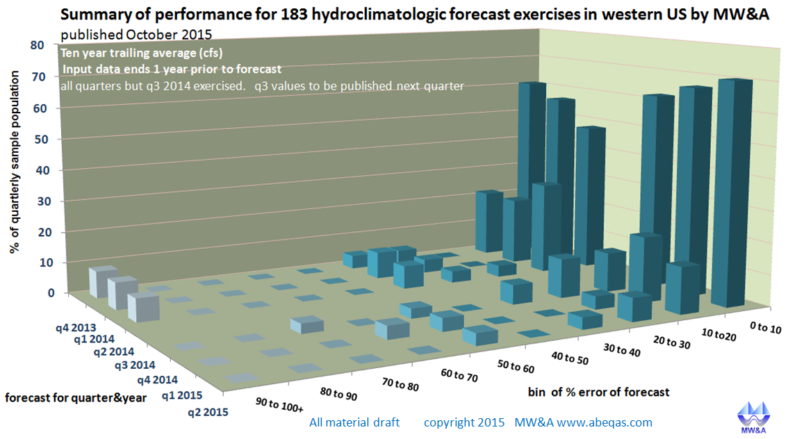
The calibration information for our case shows that our 2 year lead forecasts anticipate the ups and downs of annual stream flow very well. The magnitude of these swings as predicted by our forecast could be better. The skill is best for mean flow years and outliers are not always accurately forecast. This is not an uncommon result. We share this deficiency with the rest of the predictive methods. It appears that quantitative forecasting of extreme climate events remains beyond anyone’s solution at this time. In any event, our practice is to always disclose our skill for every forecast. Over the past 2 years, a majority of our modest regression based forecasts have shown 90% accuracy skills. See for example: http://www.abeqas.com/wp-content/uploads/2015/10/MWA_totalPerformanceUpdate2_102015.png
I had examined that Gila example at the request of a prospective client last October. Upon seeing the results, I felt it might help me to raise awareness of our high climate forecast skill by more formal comparisons to additional vendors. I developed estimation criteria which were intended to assess both transparency and skill for any vendor’s climate forecasting products. I sent out related surveys to an initial vendor list and also researched their sites. My Vendors list ranged from the Old Farmer’s Almanac variations, through the USDA NRCS SNOTEL forecasts and on to the UN IPCC Vendor along with their regionally downscaled sub models. For every case, I first reviewed the Vendor’s web site. If I failed to find disclosure of calibration reports, then I emailed the Vendor. If the Vendor responded, I updated my initial assessment with that information. If the Vendor did not respond, then I noted it, and moved on.
As with my evaluations for other vendors, I started from the UN IPCC’s high level summaries in order to generally understand the content of their climate predictions and hindcasts. It was already clear from Figure 4 for example, that we both had forecast products which could be compared in time and space.
I also assumed that their calibration (hindcast skill) products were based on GCMs which had all been run continuously through decades of simulation spans, and compared to historical decadal observations. Such practices can be seen for example in Shuhua et al. (2008). This assumption turned out to be incorrect as I detail here.
Figure 6 is adapted from Chapter 9 of WG1AR5 and represents some CMIP5 related potential calibration products. The figure shows an apparent array of long term model history matching time series products along with a representation of observation based time series of the same variable as a solid black line. In this case the variable is Temperature Anomaly deg C. However, the model simulations featured in the figure appear to include runs which received annual re-initialization to observations.

These initializations are of concern. Typically in any deterministic model, initializations of parameters are applied only once at the beginning of the time series simulation. Who would argue that this one time “initiation” is the very root meaning of the word? There would need to be extensive qualifications for any initialization to be repeated through the deterministic time frame. Were such to occur, they would be re-initializations.
Merryfield et al. (2010), provides descriptions of a GCM re-initialization practice. In this case, the document stressed that such practices at best might lead to improvements in seasonal forecasting. In other words, the predictive value of their models was not asserted at the time to reach beyond seasonal time frames of 3 months or so. The authors summarized that much of the apparent skill expressed by their forecasts came from the fact that they re-initialized the model values:
“..model sea surface temperatures (SSTs) are nudged toward the observed values during a multi-year period preceding the beginning of a forecast.”
The adjustments were needed because they could not accurately model or predict the ocean parameters sufficiently far in advance.
Yet in spite of this deficiency, gradual expansion of the initialization technique was raised throughout the GCM modeling community from seasonal to decadal forecasting time spans. These initializations came to dominate my concerns of GCM calibrations and skill reporting. They raised a host of additional concerns: Why are these parameters continually reset to match observations, when the GCMs are supposed to be predicting them in the first place? Where do they now obtain those future observations they need to keep their predictive decadal models in line? How do they leap to wholesale publications of results with high confidence?
A recent paper by Suckling and Smith (2013) , covers some aspects of this new purposing and initializing of the GCMs. Notably the article points to the practice of re-initialization of the GCMs’ boundary conditions with recent observations. The authors state in simple language that
“At present it is not clear whether initialising the model with observations at each forecast launch improves the skill of decadal forecasts… At a more basic level, the ability to provide useful decadal predictions using simulation models is yet to be firmly established.”
It’s generally agreed within model intercomparison communities, that one would not adopt model forecasts which are longer in time projection than the span of time that they are calibrated to. But in spite of such concerns, the CMIP5 program persists in delivering
“..a framework for coordinated climate change experiments for the next five years and thus includes simulations for assessment in the AR5 as well as others that extend beyond the AR5.” (Taylor et al. 2008)
This CMIP5 Design guidance document specifies the following time scales for prediction applications:
“1) near-term decadal prediction simulations (10 to 30 years) initialized in some way to ..” and
“2) long-term (century time-scale) simulations initialized from ..”
No misgivings for these forecast span time scales are communicated, other than examples such as this deep within subheadings:
Chapter 3., Part 1.2 Extend integrations with initial dates near the end of 1960, 1980 and 2005 to 30 yrs. sub section: Further details on the core runs: … “..though the whole question of initializing the climate system presents one of the biggest scientific challenges of decadal prediction” (my emphasis in bold).
The strange sentence appears to claim that their exercise is an enormous scientific challenge. I wonder if they meant to say that it might be impossible. Certainly many scientists and engineers share their UN IPCC Chapter 9 and 11 hand-wringing about non linear dynamics and chaos, including me. But if such obstacles are the real problem, then why are my forecasts so accurate?[1]
In any case, by virtue of default acceptance of the CMIP5 Design Guidance document, the re-initializing of GCM runs now appear to be the institutional cover for all of the subsequent regional decadal forecasts. Lawrence Livermore National Laboratory (LLNL) has dedicated the Program for Climate Model Diagnosis and Intercomparison (PCMDI) to maintain operational and re-initialization capability for CMIP work at:
Click to access Taylor_CMIP5_design.pdf
http://cmip-pcmdi.llnl.gov/cmip5/experiment_design.html
This program includes detailed guidance and support on how re-initializations are to be implemented. Figure 7 represents an example from Kharin et al. (2012) of four steps associated with data re-initialization.

Little is left to the imagination in this paper, except any reflection that the results are only suitable (if even then) for seasonal forecasts. The diagrams show four components to the adjustments:
1. The models are reinitialized every year
2. The reinitialized models and then bias-corrected,
3. The bias-corrected models are then trend-adjusted, and
4. The ensemble of results then are merged together.
I tried a somewhat equivalent but much looser process in an informal confirmation exercise of this initialization practice (Figure 8). I also found that the general practice does improve the perception of higher skill.

I had suggested that ocean parameters were the main subject of re-initialization. Figure 9, adapted from Gonzales et al. (2015), provides a partial explanation for this process.

The modeled Pacific Ocean surface signature patterns of temperature in both hemispheres including the equatorial zones decay rapidly, and are poorly represented by the GCMs after only a year. Re-initialization appears to apply to those temperatures, if I’m not mistaken. Only then can the models lurch forward again for a few months of potentially plausible forecasting.
An apparent appeal to bring CMIP validation and calibration practices back into line of accountable and transparent skill designation may be contained in a recent paper by Fricker et al. (2013). However the paper’s final paragraph remains disregarded:
” The ideas that we have presented are somewhat underdeveloped and they suggest several directions for further investigation. We feel that greater understanding of different types of spurious skill, their causes and their implications for evaluation would be valuable. Many more fair performance measures for ensembles that are interpreted as different types of sample could be constructed too. We shall also be interested to see if more investigations of the performance of predictions across a wide range of timescales will help to improve the quality and utility of climate predictions.”
Now that the process of CMIP validation via initializations has been institutionalized, climate change scientists apparently believe that there is no further need for actual experiments, calibration reports, or any other customary transparency. Rather, so long as the money flows, the latest observations will continue to be fed into the CMIP machine at one end. The other end will continue to emit long term climate forecasts for all locations, modalities and scales. The deployment of these inaccurate results will continue then to grow in cost and scope around the world.
It appears that without transparency demands from the public, the multi – billion dollar CMIP – blessed GMS machine will endure. What is to be done about a titanic and misguided enterprise? I recommend to start, that the skill of any climate change Vendors’ decadal forecasts, predictions, projections, and hindcasts be clearly disclosed with and without initializations. Otherwise, at the very least, the playing field is not level for small independents who offer less alarming but also more accurate solutions.
References
Fricker, T.E., C.A.T. Ferro, and D.B. Stephenson, 2013, Three recommendations for evaluating climate predictions METEOROLOGICAL APPLICATIONS 20: 246 – 255 DOI: 10.1002/met.1409
Gonzalez, P.L.M,and L. Goddard, 2015, Long-lead ENSO predictability from CMIP5 decadal hindcasts. Journal of Climate Dynamics DOI 10.1007/s00382-015-2757-0
HYDROCOIN Sweden hosted workshop in 1992 on groundwater model skill inter-comparisons
Kharin, V.V., G. J. Boer, W. J. Merryfield, J. F. Scinocca, and W.-S. Lee, 2012, Statistical adjustment of decadal predictions in a changing climate GEOPHYSICAL RESEARCH LETTERS, VOL. 39, L19705, DOI:10.1029/2012GL052647, 2012
Meehl, GA, L Goddard, J Murphy, RJ Stouffer, G Boer, G Danabasoglu, K Dixon, MA Giorgetta, AM Greene, E Hawkins, G Hegerl, D Karoly, N Keenlyside, M Kimoto, B Kirtman, A. Navarra, R Pulwarty, D Smith, D Staffer, and T Stockdale, 2009, Decadal Prediction, Can It Be Skillful? American Meteorological Society, Articles October 2009 1467 – 1485
Merryfield, W.J., W.S. Lee, G.J. Boer, V.V.Kharin, P. Badal, J.F. Scinocca, and G.M. Flato, 2010, The first coupled historical forecasting project (CHFP1). Atmosphere-Ocean Vol. 48, Issue 4 pp. 263-283
Shuhua Li, Lisa Goddard, and David G. DeWitt, 2008: Predictive Skill of AGCM Seasonal Climate Forecasts Subject to Different SST Prediction Methodologies. J. Climate, 21, 2169–2186. doi: http://dx.doi.org/10.1175/2007JCLI1660.1
Suckling, E.B. and L.A. Smith, 2013, An evaluation of decadal probability forecasts from state-of-the-art climate models. Centre for the Analysis of Time Series, London School of Economics.
Taylor, K.E., R.J. Stouffer, and G.A. Meehl, 2008, A Summary of the CMIP5 Experiment Design, Lawrence Livermore National Laboratory http://cmip-pcmdi.llnl.gov/cmip5/docs/Taylor_CMIP5_design.pdf
UN Intergovernmental Panel on Climate Change UN IPCC home page:
UN Intergovernmental Panel on Climate Change UN IPCC WG1AR5 Chapter 9 Evaluation of Climate Models 2013
Click to access WG1AR5_Chapter09_FINAL.pdf
Flato, G., J. Marotzke, B. Abiodun, P. Braconnot, S.C. Chou, W. Collins, P. Cox, F. Driouech, S. Emori, V. Eyring, C. Forest, P. Gleckler, E. Guilyardi, C. Jakob, V. Kattsov, C. Reason and M. Rummukainen, 2013: Evaluation of Climate Models. In: Climate Change 2013: The Physical Science Basis. Contribution of Working Group I to the Fifth Assessment Report of the Intergovernmental Panel on Climate Change [Stocker, T.F., D. Qin, G.-K. Plattner, M. Tignor, S.K. Allen, J. Boschung, A. Nauels, Y. Xia, V. Bex and P.M. Midgley (eds.)]. Cambridge University Press, Cambridge, United Kingdom and New York, NY, USA.
UN IPCC assessment report: 2014 Climate Change 2014 Synthesis Report Summary for Policymakers
Click to access AR5_SYR_FINAL_SPM.pdf
UN Intergovernmental Panel on Climate Change UN IPCC WG1AR5 Chapter 11 Near-term Climate Change: Projections and Predictability 2013
Kirtman, B., S.B. Power, J.A. Adedoyin, G.J. Boer, R. Bojariu, I. Camilloni, F.J. Doblas-Reyes, A.M. Fiore, M. Kimoto, G.A. Meehl, M. Prather, A. Sarr, C. Schär, R. Sutton, G.J. van Oldenborgh, G. Vecchi and H.J. Wang, 2013: Near-term Climate Change: Projections and Predictability. In: Climate Change 2013: The Physical Science Basis. Contribution of Working Group I to the Fifth Assessment Report of the Intergovernmental Panel on Climate Change (Stocker, T.F., D. Qin, G.-K. Plattner, M. Tignor, S.K. Allen, J. Boschung, A. Nauels, Y. Xia, V. Bex and P.M. Midgley (eds.)). Cambridge University Press, Cambridge, United Kingdom and New York, NY, USA.
Wallace, M.G. 2015 Ocean pH Accuracy Arguments Challenged with 80 Years of Instrumental Data.
Guest post at http://wattsupwiththat.com/2015/03/31/ocean-ph-accuracy-arguments-challenged-with-80-years-of-instrumental-data/
[1] For what it may be worth, I hope to get closer to an answer in my current graduate elective course in non-linear dynamics and chaos.
My major professor had a funny reply in discussing hydrologic models. “Nobody but the modeler believes the model output. Everyone except the experimentalist believes the empirical results.” I do have some experience with developing models for an EPA grant and even though it passed a validation it failed when applied to results from large scale trials. Several other hydrologic models also failed. Flood on the Cedar River in Iowa in 2011 or 2008 was under estimated by the state hydrologic model by about three fold. Flood ended up at 30 feet over flood stage rather than 10 feet. This model has been refined for at least 30 years by multiple groups. If the climate models are indeed being reinitiazed I would hope the modelers are able to figure out what exactly needs tweaking. Given their complexity and the number of nonlinear, partial differential equations involved, I would say good luck with that.
“No typical scientist or engineer would apply significant trust to models which do not provide transparent calibration documentation….How then do the premier United Nations Intergovernmental Panel on Climate Change (UN IPCC) GCMs provide neither model accuracy nor transparency in association with their forecasts?”
I sure hope someone raised this issue in Congressional hearings on climate change……
This is a very significant paper, if he has actually determined that they really do re-initialize the models periodicallyduring the calculation. The wording of the referenced papers is very obscure, which immediately leads to a suspicion that they are re-initializing. Tuning a code with model “dials” and settings that deal with particular special phenomena is generally considered to be bad form, and something that you only do as a last resort. Re-initializing just produces junk output.
Engineers would NEVER accept a model for an important public purpose that involved re-initializion unless it was completely disclosed, fully explained, and there was no other way to get the result. You could not really use that result to make any decisions, however, because it would be so contaminated by the re-initialization that you would never be sure exactly what ultimate result you were calculating.
I used to do international standard problems where people calculated the behavior of nuclear power plants during accident scenarios, and no one would ever do re-initialization and then claim that they had actually calculated the transient. They might complain because the boundary conditions along the path changed or were uncertain, or the instruments were not accurate, or the operators did something crazy, or something else changed along the way, but if those sorts of events were defined in the problem definition, then you had to live with them. No one gets to change the trajectory of the calculations along the way by re-initialization.
It is like saying that you can correct the trajectory of an artillery shell along its path to account for your inability to aim the cannon correctly. It may now be possible to do this, with “smart” weapons, but calculations of a physical system are not “smart bombs”, except in the most perjorative sense.
This is an extremely important post – I just wish leaders of the governments around the world were able to grasp that the conclusions of the fifth assessment report by IPCC is actually falsified by this post.
This is my favorite quote from the IPCC report regarding initializations:
«When initialized with states close to the observations, models ‘drift’ towards their imperfect climatology (an estimate of the mean climate), leading to biases in the simulations that depend on the forecast time. The time scale of the drift in the atmosphere and upper ocean is, in most cases, a few years. Biases can be largely removed using empirical techniques a posteriori. …»
(Ref: Contribution from Working Group I to the fifth assessment report by IPCC; 11.2.3 Prediction Quality; 11.2.3.1 Decadal Prediction Experiments )
Full post here:
Model biases can be largely removed using empirical techniques a posteriori!
If you combine this with how IPCC used the models and circular reasoning to excluded natural variation /long term trends:
“Observed Global Mean Surface Temperature anomalies relative to 1880–1919 in recent years lie well outside the range of Global Mean Surface Temperature anomalies in CMIP5 simulations with natural forcing only, but are consistent with the ensemble of CMIP5 simulations including both anthropogenic and natural forcing … Observed temperature trends over the period 1951–2010, … are, at most observed locations, consistent with the temperature trends in CMIP5 simulations including anthropogenic and natural forcings and inconsistent with the temperature trends in CMIP5 simulations including natural forcings only.”
(Ref.: Working Group I contribution to fifth assessment report by IPCC. TS.4.2 Surface Temperature)
Full post here:
IPPC used circular reasoning to exclude natural variation!
Within real science / engineering / technology any actions based on the IPCC report would have been suspended by discovery of these flaws.
Thanks Science or Fiction, most interesting. Glad you appreciate the bizarre and tortured language they use to explain what they did without explaining what they did.
Thanks all others as well, I’ll stay tuned and comment if I think I can add further value.
Speaking of realclimate, I did comment on this issue recently there at
http://www.realclimate.org/index.php/archives/2015/11/and-the-winner-is/comment-page-1/#comment-637826
Gavin appeared to claim at the end that they did not reset anything other than solar dynamo and volcanoes. Then the post was closed to further discussion. Gavin if you are reading this, please feel free to respond.
As a climate change modeler, Gavin is also one of a number I reached out to with my original survey, but he never responded to that.
Thanks 🙂
On a mobile now. There are more of interest towards the end of 11.2.3.1 if my memory serves me right.
“On a mobile now.”
I know I shouldn’t do it, but for some overwhelming reason I simply cannot resist the urge to say “That’s what SHE said”. 🙂
Forgive me….and now, back to science!
And THEN I notice it’s the word MOBILE and not MODEL…..:) Laugh’s on me! (And yes, I highly amuse myself all the time. lol)
D)
Brandon, you wrote earlier:
Good guesses can lead to valid findings, but nothing is jumping out of Figure 6 at me to suggest re-initializations every 5 years. It might help if you described what you’re seeing in it to suggest otherwise.
Like others who have commented, this seemed obvious, but in any case, here is more detail, already partly covered by Science or Fiction above. First, from WG1AR5_Chapter 9:
“9.3.2.3 Relationship of Decadal and Longer-Term Simulations
The CMIP5 archive also includes a new class of decadal-prediction
experiments (Meehl et al., 2009, 2013b) (Figure 9.1). The goal is to
understand the relative roles of forced changes and internal variability
in historical and near-term climate variables, and to assess the predictability
that might be realized on decadal time scales. These experiments
comprise two sets of hindcast and prediction ensembles with initial
conditions spanning 1960 through 2005. The set of 10-year ensembles
are initialized starting at 1960 in 1-year increments through the year
2005 while the 30-year ensembles are initialized at 1960, 1980 and
2005. The same physical models are often used for both the short-term
and long-term experiments (Figure 9.1) despite the different initialization
of these two sets of simulations. Results from the short-term
experiments are described in detail in Chapter 11. ”
Next, as SoF pointed out above, from WG1AR5_Chapter11, page 967:
“When initialized with states close to the observations, models ‘drift’
towards their imperfect climatology (an estimate of the mean climate),
leading to biases in the simulations that depend on the forecast time.”
Figure 11.2 below that phrase covers “CMIP5 multi-model initialized hindcasts..”
Regardless of their various claims of start dates, I remain mindful of the above statement in Chapter 9 that, “The set of 10-year ensembles are initialized starting at 1960 in 1-year increments through the year 2005”
That appears to disclose that re-initializations took place every year, not just every 5 years or every 10 years. And that is consistent with with the Kharin et al., reference. (my Figure 7).
Finally, a manual review of Figure 11.2b in comparison to my Figure 6 suggests the two are very consistent. I do believe they both come from the same re-initialized exercises.
“Next, as SoF pointed out above, from WG1AR5_Chapter11, page 967:
“When initialized with states close to the observations, models ‘drift’
towards their imperfect climatology (an estimate of the mean climate),
leading to biases in the simulations that depend on the forecast time.””
But this section is about 10-year climate model experiments. Look up at page 961, Box 11.1. After initialization, the correlation drops until the 3-year point and then begins rising again. There are several repetitions that the model’s inherent behavior takes over — but the model’s default behavior is considered to be correct for the long term. Huh, who would have thought that the IPCC’s favored models are considered by the IPCC to be correct.
https://www.ipcc.ch/pdf/assessment-report/ar5/wg1/WG1AR5_Chapter11_FINAL.pdf