By Christopher Monckton of Brenchley, David Legates, Willie Soon and Matt Briggs
Mr. Born has had another go at our paper Why models run hot, published in January 2015 (PDF here) in the Science Bulletin of the Chinese Academy of Sciences. Go to scibull.com, click on “most read articles”. and ours is the all-time no. 1 by a factor of ten. It’s a good read.
Let us begin by putting Mr. Born’s criticism into context. In essence, he is saying he would have liked our simple model to be more complex. Well, he is of course free to write his own model and get it into the reviewed literature. But our simple model, when calibrated against IPCC predictions, reproduced them faithfully when we adopted its parameter values, so, given that we made it quite explicit in the paper that we were adopting a rough-and-ready approach, we saw no reason to introduce pointless complications that would, without much increase in accuracy, have reduced the utility of our model, which is that it is accessible to anyone with a pocket calculator.
Keep it simple, stupid.
Mr. Born says the equilibrium feedback sum seems to be the only feedback sum our model uses. Well, of course it is: the impact of transient feedback values is represented in a simplified fashion by the transience fraction. That is what it is for. That is one of the many innovations in our paper, and one which is found by many to be a useful simplification.
Mr. Born draws a plot of “step responses” implied by our table of values for the transience fraction. The plot rather untidily reproduces the relevant portion of the graph from Roe (2009) from which we derived the values of the transience fraction, with one important exception. Roe’s y axis is temperature change. Mr. Born’s y axis is inadequately labeled “step response”, and it is not made explicit whether he is using a simple or normalized step response, or what the units (if any) are. He then argues with some of the points on his own graph. However, the inadequacy of the labeling and the confusing text make it difficult to understand what he means, so we cannot comment further.
In the absence of any information from the IPCC about the evolutionary profile of temperature response to different feedback regimes, we had simply used, and stated we had used, Roe’s evolutionary profile. We did not warrant it as unassailable, and we did say that people were free to take their own values, and we did additionally provide worked examples so that, at least for the next century or two, values sufficiently close to the IPCC’s values could be readily reproduced, and in our own centennial worked examples on all six RCP scenarios we used values close to those implicit in the IPCC’s transient-sensitivity predictions.
Next Mr. Born has a long and unnecessary excursus on whether the Planck parameter is a feedback or not. As our paper explains, echoing Roe, with whom our lead author had discussed this question, it is better understood as part of the reference frame for climate-sensitivity calculations.
In particular, Mr. Born would have liked a more complicated treatment of our transience fraction – i.e., the fraction of equilibrium climate sensitivity achieved in a given year after a stimulus has been applied to the climate. He would have preferred us to convolve entire time sequences instead of carrying out the simple multiplication that is at the heart of our model. However, the IPCC itself uses the simple multiplication method from time to time, and we provided worked examples to show that that method reproduced the IPCC’s climate sensitivity when its own parameters, specifically including feedback values, were input to our model. And we cited IPCC passages where the simple multiplication method was used. Indeed, it is often used in determining sensitivity from general-circulation models too: see e.g. Hansen (1984). Once again, Mr Born’s quarrel is not with us but with the IPCC and with the modelers. The point about a simple model is that it does things the simple way, for better or worse.
In logic, a model is a simplification and a simplification is an analogy, and every analogy breaks down at some point. Mr Born should feel free to make the model more complex if he wants: our paper is the manual for it, so he can simply read the manual and replace anything he does not like with something more complicated of his own. But his entire post would make scarce a jot or tittle of difference to equilibrium sensitivity, which was the principal focus of our paper.
Equilibrium sensitivity is the warming that might be expected to occur by the time the climate had settled back to a steady state in response to a direct forcing followed by the complete action of all temperature feedbacks consequent on that forcing. Now, it is a matter of definition that at equilibrium the transience fraction must in all cases be unity. So the vast majority of our paper that treats of equilibrium sensitivity is entirely unaffected by any doubts about the values one might choose to adopt for the transience fraction at various points before equilibrium is reached.
The remainder is not much affected either, for our centennial transience fractions are very close to those of the IPCC. If Mr. Born does not like them, yet again his quarrel is with the IPCC and not with us.
Mr. Born’s post, therefore, deals with a secondary aspect of our paper, and one in which just about any defect caused by what he may consider to have been an inappropriate choice of transience fractions by us (or by Roe before us) would in all realistic circumstances be dwarfed and swamped by uncertainties as to the values of both forcings and feedbacks. The recent news that the models and the IPCC have been artificially boosting climate sensitivity by adopting very large but unphysical negative aerosol forcings – something I have long suspected – is a case in point.
In the climate, a temperature feedback is an additional forcing, denominated in Watts per square meter per Kelvin of direct temperature change caused by the original forcing. The classic temperature feedback is the water-vapor feedback. As the atmosphere warms, by the Clausius-Clapeyron relation it can carry near-exponentially more water vapor, a greenhouse gas.
So the IPCC assumes that merely because the atmosphere can carry near-exponentially more water vapor it must do so. That is a convenient assumption, because it allows the IPCC immediately to double the direct warming expected from adding CO2 to the atmosphere. However, it is by no means clear that the water vapor in the atmosphere is increasing. For instance, the ISCCP satellite data show no change at all in recent decades except in the climatically crucial mid-troposphere, where the column water vapor appears to have declined somewhat – precisely the opposite of what the IPCC would like us to believe ought to happen.

Another example: Spencer and Braswell (2010, 2011) found cloud feedbacks negative, not – as the IPCC thinks – quite strongly positive. Both they and Lindzen & Choi (2009, 2011) found the feedback-sum net-negative. Considerations like these simply drown out any supposed defects in the choice of the transience fraction.
The point here is one that we made in the paper: the values of individual feedbacks, and even their signs, cannot be either directly measured by any empirical method or inferred to a sufficient precision for climate-sensitivity calculations by any theoretical method. They are guesswork. They cannot be empirically distinguished from one another or even from the forcings that generated them.
And the curve along which the influence of feedbacks on temperature is expected to evolve is likewise guesswork – and guesswork so problematic that the IPCC does not even attempt to plot it, except in graphs the size of a postage stamp in AR4, p. 803, Table 10.26. The IPCC would have us to believe that half of the warming caused by a forcing amplified by feedbacks should have occurred in the first century after the forcing, with the rest of the warming coming through only after hundreds (or, in the high-sensitivity case) thousands of years. They may – or may not – be right. But our values for the transience fraction are broadly in line with this consideration, after appropriate allowance has been made for the fact that time to equilibrium increases with the feedback sum.
We took, and said we took, a rough-and-ready approach, using a profile of feedback evolution over time taken from Roe (2009). And, notwithstanding a snidish comment from Mr Born that scientific papers ought to be rigorous, implying that ours was not, we had made it quite plain that Roe was using a pulse, not a growth of forcing over time. Rigor, in any paper concerning a model, requires up-front disclosure of what was done. We did that.
So having nailed down the upper bound of the transience fraction, which is by definition unity, let us look at the lower bound, which – if feedbacks are net-positive – is simply the ratio of the Planck sensitivity parameter 0.31 Kelvin per Watt per square meter and the equilibrium sensitivity parameter, which is in turn simply the equilibrium climate sensitivity in Kelvin divided by the original direct forcing in Watts per square meter.
All the user of our model has to do is set the transience fraction at 1 for equilibrium, run the model with all other parameters chosen by him to determine equilibrium sensitivity and hence the equilibrium sensitivity parameter, divide the Planck parameter by the equilibrium sensitivity parameter and, bingo, the instantaneous or initial value of the transience fraction in response to a direct forcing may be determined.
We actually provide handy equations in the paper for understanding these relationships. You will not find anything like so clear in the IPCC’s documents.
But what about the years in between instantaneity and equilibrium? Now, the IPCC has been criticized by its expert reviewers for not providing an explicit evolutionary path for climate sensitivity. However, one can deduce from the IPCC’s values for transient sensitivity that after 100 years about half of the equilibrium sensitivity will have occurred. We provided worked examples in our paper to demonstrate this. Indeed, that consideration alone is enough to show that the transience fractions in table 4 of our paper, about which Mr Born also seems to complain, are in the right ballpark.
Mr. Born, however, expects us to have done what the IPCC has not done. As so often, his quarrel is not with us but with the IPCC. For he has repeatedly complained that we had not explained how we had determined our values for the transience fraction. Nor does the IPCC.
Well, at least Mr. Born now knows what the instantaneous, 100-year and equilibrium values of the transience fraction are, for any given situation. And all of this was explained in our paper.
But what of the values in between? Mr Born opens his article by saying our lead author had “turned down” his “request” to explain how we determined the values of the transience fraction. He had said much the same in a very late-in-the-day and not very courteously expressed comment on our lead author’s response to his earlier article:
“Many of us were interested in precisely how Monckton et al. inferred the Table 2 values from the Gerard Roe paper. The explanation should have been easy to give. Yet the authors, or at least Lord Monckton, insisted on withholding that information.”
To allege that authors of a scientific paper have deliberately withheld requested information is to make a very serious allegation of professional misconduct. That is the allegation that Mr Born has now made twice, and in the bluntest terms.
So let us be clear as to the facts. Mr. Born at no time contacted any of us to ask for the information he now says we are “withholding” and “refusing to provide”. He must withdraw that allegation, and be very careful in future not to repeat it.
Now, Mr Born may argue that he had, at the foot of a previous comment thread, asked for the information he said we were “withholding” and now says we are “refusing to provide”. He will see, not far below his comment on that thread, the words “Comments are closed.” So we were not able to reply to him. We have no idea why comments were closed: but they were closed. It is not unreasonable, we think, to expect Mr Born to be a great deal more rigorous in verifying his facts before making unpleasant allegations that we have withheld or refused to supply information for which not one of us had received a request from him. Nor can he maintain that he had no email address for us: our lead author’s email address is published in our paper.
Notwithstanding Mr. Born’s discourtesy, we now provide the information requested.
Not all temperature feedbacks operate instantaneously. Instead, feedbacks act over varying timescales from decades to millennia. Some, such as water vapor or sea ice, are short-acting, and are thought to bring about approximately half of the equilibrium warming in response to a given forcing over a century. Thus, though approximately half of the equilibrium temperature response to be expected from a given forcing will typically manifest itself within 100 years of the forcing, the equilibrium temperature response may not be attained for several millennia (see e.g. Roe, 2009; Solomon et al., 2009).
In our model, the delay in the action of feedbacks and hence in surface temperature response to a given forcing is accounted for by the transience fraction. For instance, it has been suggested in recent years that the long and unpredicted hiatus in global warming may be caused by uptake of heat in the benthic strata of the global ocean. The construction of an appropriate response curve via variations over time in the value of the transience fraction allows delays of this kind in the emergence of global warming to be modelled at the user’s will.
In Roe (2009), a simple climate model was used, comprising an advective-diffusive ocean and an atmosphere with a Planck sensitivity 1.2 , the product of the direct radiative forcing 5.35 ln 2 = 3.708 Watts per square meter in response to a CO2 doubling and the zero-feedback climate sensitivity parameter 0.3125 Kelvin per Watt per square meter. The climate thus defined was forced with a 4 Watts per square meter pulse at the outset, and the evolutionary curve of climate sensitivity was determined and plotted.
In our paper, Table 2 gives approximate values of the transience fraction corresponding to equilibrium feedback sums f ≤0 and f = 0.5, 1.3, 2.1 and 2.9. Where the equilibrium feedback sum is less than or equal to about 0.3, the transience fraction may be safely taken as unity: at sufficiently small f there is little difference between instantaneous and equilibrium response. For f on 2.1 [1.3, 2.9], the value of the transience fraction is simply the fraction of equilibrium sensitivity attained in a given year after the initial forcing, as shown in Roe’s graph, reproduced at fig. 4 of our paper.
It is not possible to provide a similar table for values of f at equilibrium given in IPCC AR4 or AR5, since IPCC provides no evolutionary curve similar to that in Roe’s graph.
There. All is now explained, and in quite some detail. Mr Born may be tempted to ask why I did not explain all this before. The answer, of course, is that we did. All five of the preceding paragraphs are taken straight from our paper. He has been asking us to explain what is already explained, fully, in our paper. He has alleged, time and again, that we did not explain how our values for the transience fraction were arrived at. But it will be seen that we had taken considerable trouble over that, so that everyone could understand the basis for our own approximate values of the transience fraction, and could choose their own values if they preferred.
Mr. Born then takes us to task for basing our values of the transience fraction on Roe’s model, on the ground that that model was forced by a pulse rather than by small annual increments. Over the short term (i.e. the next couple of hundred years), our values of the transience fraction are manifestly consistent with those of the IPCC – see the worked examples in our paper. Yet again, therefore, Mr Born is arguing with us when he should be arguing with the IPCC. We are using its methods. It uses pulse analysis as well as step-by-step forcings in its modelling. Each method has its merits and demerits. If our model has what Mr Born considers to be defects at the margins, welcome to modeling.
If you want perfection, wait and do a hindcast. Even then, disentangling the natural from the anthropogenic contributions will be no easy task.

Mr. Born says we were not right to assume that for negative feedbacks the transience fraction could be safely taken as unity. Do the math. For a feedback sum on [-1.6, +0.32] Watts per square meter per Kelvin, equilibrium climate sensitivity falls on the remarkably narrow (and remarkably harmless) interval [0.8, 1.3] K.
Look at the curve of equilibrium sensitivity against loop gain in our paper. See for yourself. It at once becomes apparent that little error can arise from assuming the transience fraction is unity in such circumstances. But Mr. Born is free to adopt his own more precise values if he wants. They will make scarcely any difference to climate sensitivity – and, of course, all sensitivities in response to a net-negative feedback sum will be a third of the IPCC’s sensitivities, or even less. Respice finem.
Mr. Born says users of our model should adopt our transience values with caution. Well, of course they should. We made it quite clear once in the text and twice in Table 2, that the values for the transience fraction were stated to be “approximate”. Given the unknowns, of course they were approximate. How useful to be able to end on a note of agreement.
Addendum
An anonymous contributor, one “Phil.” [a professor at Cornell -Anthony], has twice alleged in comments that the appendix to our paper, which was cut at the last minute by the editors on grounds of space, and which among other things provided a more explicit but still simple mathematical discussion of feedback-induced non-linearities, had never existed.
Now, our lead author had invited “Phil.” to email him if he wanted a copy of the appendix. Instead, “Phil.” merely repeated the allegation that our lead author had lied in saying there was an appendix. We can now confirm that neither “Phil.” nor anyone contacted any of us to ask for a copy of the appendix before he repeated his allegation. We can also confirm that the appendix has not been hastily cobbled together ex post facto but was indeed submitted with our paper and approved by our three diligent reviewers.
The serious and unfounded allegations both of Mr. Born and of “Phil.” are the sort of thing that those of us who have dared to question the party line they cherish must endure daily. Just ask our distinguished co-author Willie Soon, who has been hounded unmercifully throughout the media in the months following publication of our paper for having allegedly failed to disclose the identity of one of his funders, when the contract between his observatory and the funders, negotiated by them and not by him, obliged him not to mention the funder’s identity. He was blameless, but that has not prevented the usual suspects from mounting an expensive, organized, and persisting campaign of vilification against him.
Neither he nor any of us will be discouraged by the continuous nastiness to which we are subjected. So vile has been the treatment of sceptical researchers by the climate extremists that third parties looking in on this debate can see that on the skeptical side there is at least an attempt at rational discussion, while from the true-believers there is little but hate speech and false allegation piled upon false allegation.
That is no small part of the reason why the climate extremists are losing the argument. They are not conducting one.
APPENDIX 1
Further development of the model
The model may readily be further developed to increase its sophistication, though such developments are beyond the scope of the present paper. For instance, an additional factor might be included in Eq. (1) to represent any desired contribution from anthropogenic forcings.
The model might also be made one-dimensional, by representing the latitude. One-dimensional energy-balance models (see [49] for an overview), originally developed by [50-51] and extended by [52-53], have been widely used to introduce students to climate modeling and to examine some peculiarities of the climate system. Some of the more interesting issues that appear when latitude is taken into account are polar amplification of sensitivity to a forcing, the snowball/snow-free bi-stability [54] and the small ice-cap instabilities [55] that arise from the positive ice-albedo feedback.
A one-dimensional model starts with (1) and, at each latitude φ, expresses the albedo α of the Earth and its clouds, its effective temperature TE, and the distribution of solar irradiance S as functions of x = sin φ. The one-dimensional model also implicitly assumes that the northern and southern hemispheres are reflections of one another with no net heat flux across the equator. To resolve the latitudinal dimension, the model may be grid-based, as in [52-53], or based on Legendre polynomials (as in [54]).
The model, however formulated, requires a further equation to describe the meridional or poleward transfer of heat. This energy-flux divergence D is proportional to –![]() 2T. Using Fick’s Law of Diffusion in (A1.1), it is expressed by
2T. Using Fick’s Law of Diffusion in (A1.1), it is expressed by
![]() , | x = sin φ (A1.1)
, | x = sin φ (A1.1)
where the diffusion coefficient, ![]() , representing the poleward transfer of energy via oceanic and atmospheric advection, is a tunable parameter that yields a realistic equator-to-pole temperature gradient and can be simplified to render it independent of latitude, with a customary value ~0.65 W m–2 K–1. In [56] a diffusion coefficient is suggested that is dependent on x2 (consistent with the diffusion coefficient in [50]) so that tropically-averaged motions are better described,
, representing the poleward transfer of energy via oceanic and atmospheric advection, is a tunable parameter that yields a realistic equator-to-pole temperature gradient and can be simplified to render it independent of latitude, with a customary value ~0.65 W m–2 K–1. In [56] a diffusion coefficient is suggested that is dependent on x2 (consistent with the diffusion coefficient in [50]) so that tropically-averaged motions are better described,
![]() , (A1.2)
, (A1.2)
where ![]() is the second Legendre polynomial and
is the second Legendre polynomial and ![]() ,
, ![]() are tunable parameters [see also 57]. Use of the second Legendre polynomial is fortunate in that
are tunable parameters [see also 57]. Use of the second Legendre polynomial is fortunate in that ![]() should decrease toward the pole, as it does in (A1.2). Given the complicated motions of the atmosphere and ocean that transport the energy poleward, such diffusive approximations are conceptually appealing but may not be entirely physically-based [54]. Formulation of diffusion using (8) introduces a term that varies as a function of the equator-to-pole temperature distribution which, necessarily, will alter the temperature response ΔTt to anthropogenic radiative forcings, thereby changing the response in Eq. (1). Specifically, addition of latitudinal diffusion will affect not only the transience fraction, rt, since the impact of diffusive heat transport and its response to ΔT will change the response time to anthropogenic forcing, but also the equilibrium climate-sensitivity parameter, λ∞.
should decrease toward the pole, as it does in (A1.2). Given the complicated motions of the atmosphere and ocean that transport the energy poleward, such diffusive approximations are conceptually appealing but may not be entirely physically-based [54]. Formulation of diffusion using (8) introduces a term that varies as a function of the equator-to-pole temperature distribution which, necessarily, will alter the temperature response ΔTt to anthropogenic radiative forcings, thereby changing the response in Eq. (1). Specifically, addition of latitudinal diffusion will affect not only the transience fraction, rt, since the impact of diffusive heat transport and its response to ΔT will change the response time to anthropogenic forcing, but also the equilibrium climate-sensitivity parameter, λ∞.
The model may also be developed to represent non-linear temperature feedbacks. Where feedbacks are non-linear (see [38] for the derivation), Eq. (4) becomes Eq. (A1.3):
![]() . (A1.3)
. (A1.3)
In the general case, therefore, the linear-feedback system-gain relation Gt = (1 – gt) –1 becomes Eq. (A1.4):
![]() | ξ = 0 where feedbacks are linear. (A1.4)
| ξ = 0 where feedbacks are linear. (A1.4)
References
38. Roe G (2009) Feedbacks, timescales, and seeing red. Ann Rev Earth Planet Sci 37:93–115
49. Bódai T, Lucarini V, Lunkeit F et al (2014) Global instability in the Ghil-Sellers model. Clim Dyn [in press]. doi:10.1007/s00382-014-2206-5
50. Budyko MI (1969) The effect of solar radiation variations on the climate of the Earth. Tellus 21:611–619
51. Sellers WD (1969) A global climatic model based on the energy balance of the earth-atmosphere system. J Appl.Meteorol 8:392–400
52. North GR (1975) Theory of energy-balance climate models. J Atmos Sc. 32:2033–2043
53. Ghil M (1976) Climate stability for a Sellers-type model. J Atmos Sci 33:3–20
54. North GR, Cahalan RF, Coakley JA Jr (1981) Energy balance climate models. Rev Geophys Space Phys 19:91–121
55. North GR (1984) The small ice cap instability in diffusive climate models. J Atmos Sci 41:3390–3395
56. Lindzen RS, Farrell B (1977) Some realistic modifications of simple climate models. J Atmos Sci 34:1487–1501
57. Schneider EK, Lindzen RS (1977) Axially symmetric steady-state models of the basic state for instability and climate studies, Part I, Linearized calculations. J Atmos Sci 34:263–279
I distinctly recall Mr. Born’s article where he stated that the authors of this paper were withholding information he had asked for. If it is indeed true that Mr Born did not even bother to email the authors for the information, then such behaviour is utterly contemptible. I’d be very upset also.
Worse, if the information he alleges was being withheld IS actually in the paper…
The water vapour column graph from the climate4you site is an interesting one and shows more about feedbacks than the models ever will. first the graph shows a net loss in water vapour in the higher troposphere, so yeah sure there is no hot spot etc, but the 1000mb show a slight increase in recent years (see other graphs on the climate4you site climate/clouds page/specific humidity). the question here is, where is the temp increase in the lower troposphere?
RSS etc show no increase in temps in the TLT for the past 18 years, and there is MORE water vapour there. if you look at the other graphs on the page, the answer is clear. recently the cloud cover has increased, especially in the tropics.
Mobihci is quite right about cloud cover. From 1983-2001, according to Pinker et al., 2005, there was quite a dramatic reduction in cloud cover, causing a forcing that dwarfed any anthropogenic forcing. However, when I wrote a paper pointing this out, the revisionists got to work and now say there was more cloud cover than Pinker thought. However, the ISCCP data again agree with Pinker, showing quite an appreciable increase in cloud cover at the beginning of the new millennium, since when there has not been much in the way of global warming.
mobihci
April 5, 2015 at 6:44 pm
“RSS etc show no increase in temps in the TLT for the past 18 years, and there is MORE water vapour there. if you look at the other graphs on the page, the answer is clear. recently the cloud cover has increased, especially in the tropics.”
——————————–
Hello mobihci.
A very good point.
Now if I had to try and understand this, I have to consider the link or the coupling between warming and humidity by a simple approach.
More energy more of what can contain it, the humidity.
More energy introduced and circulating in the system more humidity to allow for as such.
Considering the tropics in a climate atmospheric angle the humidity varies but very little, and the lower humidity will happen to be at the very point that the end of the Ice Age kick-starts with the higher humidity reaching when the end of the Interglacial Optimum kick-starts, hypothetically.
In between these two points in time the RF goes up, atmosphere warms (not only because of RF) and the humidity goes up.
But funny enough there seems to be a point where the increased humidity does not support or allow any more warming……..many here explain it as through a negative feedback of humidity to the RF, if I am not wrong……..contrary to a positive feedback of humidity to the atmospheric warming as claimed in the case of AGW.
No matter how big, Atmosphere is not limitless, it has his limit, therefore so does the humidity and the warming, in principle.
Meaning that at a certain point the further increase of humidity will prohibit the accumulation of warming in the system, regardless of how much energy the Atmosphere is subjected to. It will lead to a balancing out first, where for any unit of energy “entering” at that point in time one energy unit will leave and depart to the space out there.
Then beyond that point further increase of humidity it will cause cooling by leading to a loss of more than one energy unit for each end every energy unit “entering” the system, getting at somewhere of the max of two lost for each one “entering” till it gets to the point that humidity starts lowering.
My guess is that the relation of humidity to RF by this angle suggest that at 360 ppm due to the humidity the warming stops, and according to our present situation the cooling solely due to the RF-humidity relation will last till somewhere the 460 ppm is reached.
I could go on and on with this rumblings but I would not like to be boring ……
cheers
hi whiten,
yeah, it is probable that there is an upper limit, however recent history (last 100k years) shows much warmer temps than now with little difference in continental arrangement. I tend to believe that the modulation of the cloud cover feedback is the main reason for climate shifts. what is modulating the cloud cover is probably the main question there. eg sun, ocean cycles etc.
mobihci
April 6, 2015 at 12:25 am
I tend to believe that the modulation of the cloud cover feedback is the main reason for climate shifts. what is modulating the cloud cover is probably the main question there. eg sun, ocean cycles etc.
—————————————–
Perhaps you misunderstood my point.
I was not arguing or trying to show my believe or my opinion on what the actual cause or main reason for climate change or climate shifts, even that it may look that way.
Let me paste copy from my above reply to you :
“……..and according to our present situation the cooling solely due to the RF-humidity relation will last till somewhere the 460 ppm is reached.”
As I said “the cooling solely”, which actually means a temporary cooling due to RH-humidity relation.
At most it can be considered as a climate response to the condition we are in recently, the last 300 years.
As I tried to explain it in my previous reply, once that condition reached, the limit of humidity, regardless at what actual warming point the Atmosphere is (less or more than anywhere of the last 400K years), there will be no further warming, and even cooling may be starting, depending on the RF and mainly in the initial cause or initial main reason for such a condition to arise.
For some reason in the last 300 years the CO2 emission has sharply risen and has reached a ~400ppm and also the temp has sharply risen up by ~more then a 1.0C.
Normally for such a sharp CO2 increase it takes about a 5K years and for the temp increase at 1.C it will take about 3K years.
Now I am not claiming I am right and you are wrong, just kind of expressing my thoughts.
Sorry that we are on different opinions…….and of course you could be right……or we simply could both be wrong……but I think it will be difficult to expect that we both right with our opinions.
Thank you for your reply, appreciated…:-).
cheers
Excellent reply Lord Monckton. Absolutely crystal clear.
Shame on Joe Born and Phil for their dishonest allegations and deliberate misleading attempts. And contempt for Mosher who has as usual shown what a waste of time he is.
If Mosher has anything to say he should say it, but he never seems to say anything. He types a lot of words, but they never say anything.
I pointed out to Monckton that there was no appendix to the scibull paper in January and he said that he would “send a copy”. Nothing dishonest or misleading, we now have the appendix.
So now that your wild goose chase is over care to have anything intelligent to say about the paper?
Clearly it was not a ‘wild goose chase’, since Monckton has provided the appendix in response to my request.
It was a wild goose chase as you dodged the question about whether you have anything intelligent to say about the paper. That’s something which has been conspicously absent from your posts on this subject.
Apparently you don’t know what a ‘wild goose chase’ is. I had my say in January.
Let’s try that again: values from the Roe paper “[in] a manner that their paper does not make entirely clear.”
 wasn’t clear enough. But no explanation was forthcoming, so I wrote another post.
 for
for  : a higher early-year temperature response to a forcing could imply a lower equilibrium response to it. Specifically, the
  curve intersected the
  and
and  curves. I brought the reader’s attention to that problem as follows:
Let’s review the bidding, shall we?
The title of my first post on the subject was “Reflections on Monckton et al.’s ‘Transience Fraction.’” I said in that post’s first paragraph that their paper “obscures the various factors that should go into selecting that parameter.” I further said that Monckton et al. had inferred their Table 2
It taxes even my credulity that this left unobvious my belief that Monckton et al.’s determination of the transience fraction
Fig. 1 of that post illustrated the implausible consequence of the authors’ assuming
Rather than address that issue, the authors quibble about nomenclature:
It’s hard to escape the conclusion that the authors are being willfully obtuse. “Step response” is a concept well known to those qualified to lecture us about feedback, as Lord Monckton repeatedly does. Still, If it really was foreign to them, they could have Googled it.
Moreover, the text accompanying that plot described it in the following manner:
And don’t forget that the stimulus was explicitly referred to as “a step in forcing.” All that leaves little to the imagination regarding what “step response” meant in that case.
Now, by contending that I misrepresented things in saying that the authors had not been forthcoming about Monckton et al.’s transience fraction, the authors have endeavored, with some success apparently, to divert attention from their again evading the issue. But let’s consider the facts.
That post was hardly the first time that the issue of implausible $r_t$ values had been raised. Zeke Hausfather reported several weeks ago that he had raised it at Climate Etc. Lord Monckton merely responded with an oh-no-you’re-wrong type of argument: “We assume, correctly, that the transience fraction is unity where temperature feedbacks are zero.” To help him see his error, I responded thus to his statement:
Note that I again told him what a “step response” was. Note also that this occurred on March 15, at least nine days before the closing of comments on which the authors blame their failure to respond. values, yet that table gives values for five curves. One might therefore speculate that the implausible
  values resulted from the way in which the authors changed three into five. But why should we speculate? The authors presumably know how they got the curves. Why make that an exercise in pulling teeth. Why insist that inquirers jump through hoops to get the answer?
 should be revised accordingly. Or they could have said something else.
Then, perhaps putting too fine a point on it, I actually supplied code by which a plot similar to that in the subsequent post could be created, explicitly using the “step response” nomenclature and moreover inviting Lord Monckton’s attention to the specific issue by asking, “Doesn’t it seem odd that the f = 0 curve intersects the f = 0.5 and f = 1.3 curves?” Note that this was March 16, at least eight days before the closing of comments. And Lord Monckton was commenting on the same thread days later.
Tell me again, who’s misrepresenting things here?
Now, there were one or arguably three curves on the Roe plot from which the authors ostensibly obtained their Table 2
How might they have answered? Well, perhaps they could have said that, yes, that result seems implausible, but here’s why it really isn’t. Or they could have said that, yes, that was a transcription error; the real values should have been such and such—and, by the way, our §8.4 conclusion based on unity
What did they say in the event? Well, apparently all four authors put their heads together and, astonishingly, this seems to be the best they could do:
Go ahead, read that again. What did they say? value by blandly assuming that “Where the equilibrium feedback sum is less than or equal to about 0.3, the transience fraction may be safely taken as unity,”—even though doing so gives a higher equilibrium response for a lower transient response—and they are silent about their
  curve.
 values could “safely be taken as unity.” No explanation of where the
  curve came from. No explanation of how a higher transient response could, as the
  curve implies, result in a lower equilibrium response.
All they said, after all this time, is that they got three of the curves from Roe, they got the
No explanation of how they inferred from Roe that unity-
That’s what in their circles passes for a complete explanation “and in quite some detail”? That’s what passes for rigor? That’s the best they can do?
For the sake of transparency, are you “Phil” the professor at Cornell? What is your real name and profession?
Good question, Dr.Strangelove. And I wouldn’t hold my breath waiting for a straight answer.
The irony of two people who post under pseudonyms asking that question! As I have said here on more than one occasion, I stopped posting to blogs under my full name after a denial of service attack rendered my email communication unusable and caused significant problems (not WUWT).
dbstealey April 5, 2015 at 9:26 pm
Christoph Dollis,
Yes, there are lotsa folks named Phil.
Indeed, but as far as I know I’m the only one who posts here as ‘Phil.’?
To repeat, I am not, and never have been, a professor at Cornell.
I have never asked Anthony Watts to post my paper on this website. Since you did, it is only proper to give your real name and profession, unless that would discredit your reputation. The people you are accusing to be wrong have real names (Monckton, Legates, Soon, Briggs) and real professions (professor and physicist)
Non-technical readers cannot follow the technical arguments of both sides and would want to know if they are hearing from Phil the professor or Phil the troll. Hiding your true identity would only boost suspicion of the troll and his gibberish jargons.
Dr. Strangelove April 6, 2015 at 8:16 pm
I have never asked Anthony Watts to post my paper on this website. Since you did, it is only proper to give your real name and profession, unless that would discredit your reputation.
What on earth are you talking about, what paper of mine did I ask Anthony to post here?
The people you are accusing to be wrong have real names (Monckton, Legates, Soon, Briggs) and real professions (professor and physicist)
So do I, but I didn’t accuse them of anything here
Non-technical readers cannot follow the technical arguments of both sides and would want to know if they are hearing from Phil the professor or Phil the troll.
It isn’t that technical, Monckton told me to read the Appendix to the paper, I told him there wasn’t one (go look at the paper: http://www.scibull.com:8080/EN/abstract/abstract509579.shtml). Monckton offered to send me a copy of the Appendix, I asked him to post it here instead, which he did.
For some reason the authors posted here today:
An anonymous contributor, one “Phil.” [a professor at Cornell -Anthony], has twice alleged in comments that the appendix to our paper, which was cut at the last minute by the editors on grounds of space, and which among other things provided a more explicit but still simple mathematical discussion of feedback-induced non-linearities, had never existed.
That is not true, I did not claim that the Appendix never existed, merely that there was not a published Appendix so I couldn’t take Monckton’s advice and read it! I actually asked Monckton for a link to it, Monckton seemed surprised that it wasn’t in the journal, so I assumed he hadn’t been told.
Now, our lead author had invited “Phil.” to email him if he wanted a copy of the appendix. Instead, “Phil.” merely repeated the allegation that our lead author had lied in saying there was an appendix.
Again not true, Monckton did indeed post:
Monckton of Brenchley April 3, 2015 at 3:53 am
“In response to Phil., if he emails me I will send him the appendix”.
To which I replied:
Phil. April 3, 2015 at 9:28 am
“Please just post it here so that everyone can have access to it”.
Which is what he did.
So ‘Phil’ a.k.a. ‘Joe Born’ is denying he is Joe Born. And ‘Phil” or ‘Joe Born’ is denying he wrote the Guest Essay by Joe Born. How many Joe Borns are there anyway? And ‘Phil’ or ‘Joe Born’ is denying he accused Monckton et al of anything. Perhaps the guy was just writing gibberish that has no bearing whatsoever on the paper of Monckton et al. I’m a bit confused why ‘Phil’ is answering on behalf of ‘Joe Born.’ Perhaps one or both are fictitious trolls and this whole thing is just a prank.
Dr. Strangelove April 6, 2015 at 9:42 pm
So ‘Phil’ a.k.a. ‘Joe Born’ is denying he is Joe Born. And ‘Phil” or ‘Joe Born’ is denying he wrote the Guest Essay by Joe Born. How many Joe Borns are there anyway? And ‘Phil’ or ‘Joe Born’ is denying he accused Monckton et al of anything. Perhaps the guy was just writing gibberish that has no bearing whatsoever on the paper of Monckton et al. I’m a bit confused why ‘Phil’ is answering on behalf of ‘Joe Born.’ Perhaps one or both are fictitious trolls and this whole thing is just a prank.
You appear to be very confused, you addressed questions specifically to me and now it appears you thought you were addressing them to ‘Joe Born”!
Just to clarify, I am not ‘Joe Born’, as far as I know he is exactly who he says he is. Since Anthony requires people who contribute articles on WUWT to be properly identified I am sure that’s his correct name.
My first post was addressed to Joe Born. For some mysterious reason, you answered it. Perhaps you also thought you were Joe Born. I’m not the only one confused. Apparently Anthony thought ‘Phil’ is a professor at Cornell, which you denied assuming you are really Phil or Joe Born. Sure you are not Joe Born. You are just a mysterious guy answering on behalf of Joe Born.
Dr. Strangelove April 7, 2015 at 8:21 pm
My first post was addressed to Joe Born. For some mysterious reason, you answered it.
So you asked Joe Born “For the sake of transparency, are you “Phil” the professor at Cornell? What is your real name and profession?
Since Anthony responded: “Phil.” [a professor at Cornell -Anthony] why on earth would you address your question to Joe, particularly given the site policy on transparency for guest posters?
Since you were making such a radical departure perhaps you should have actually addressed the question to Joe to avoid confusion?
Mr Born continues to be unsatisfactorily disingenuous. He said we had withheld, et separatin turned down his requests for, information. He had not written to any of us with any such request.
In our paper, and again in the head posting here, we explain why a transience fraction of unity is a respectable approximation for negative or barely positive closed-loop gains. In both places we even provided a clear diagram.
As many have pointed out here, Mr Born owes us an apology.
“As many have pointed out here, Mr Born owes us an apology.”
Yes, Lord Monckton has gulled the easily led into embracing his novel rule of etiquette that blog conversations must turn to email whenever a request for information is involved. That’s the level of independent thinking that explains the last U.S. presidential election results.
Again we see Lord Monckton flee to form when he gets outmatched on substance.
Joe,
Let me get this straight. So you accuse the authors of the paper from withholding information in a way that is clearly mischievous. You then admit you never bothered to write directly to the authors. On top of that you now boldly declare that what you’ve done is perfectly acceptable. Irrespective of any technical merits there may have been in your arguments it’s become perfectly clear you’re something of a weasel.
Venter April 6, 2015 at 1:58 am
Lord Monckton, the second line of your reply has come scrambled with parts cut off..
It looks like Monckton has made a typo for the legal term, ‘et separatim’, that cell phone again.
Mr Born continues to be lamentably disingenuous. I am not taking him to task for not having emailed me: I am taking him to task for having falsely alleged that I had “withheld” information or “turned down” a request from him for information, when he had not in fact made any request for that information to any of us and when the information was available in our paper in the first place. He has lost a great deal of credibility by not apologizing as he should have done.
In view of your saying “barely positive closed-loop gains” and your second graph at the top, I think you are still confusing “closed-loop gain” with “loop gain”.
Lord Monckton, the second line of your reply has come scrambled with parts cut off..
Don’t myself think that Lord Monckton was wrong to point out the unjustifiable claims of his detractors. It is a sure sign of weakness in a debate when those unable to produce a suitable reasoned scientific counter argument to a paper have to resort to personal attacks.
Perhaps Lord Monckton should reconsider the possibility of perusing litigation, as this would deter others from using this bad practice in the future. The case would also gain even more publicity than has already been successfully achieved.
BTW, have you read the latest paper by Ferenc Miskolczi, published in Development in Earth Science Volume 2, 2014 – “The Greenhouse Effect and the Infrared
Radiative Structure of the Earth’s Atmosphere”, which broadly supports your neutral assumption on climate feedback. Full paper here…
http://www.seipub.org/des/Download.aspx?ID=21810
A paper published in Journal of Climate, 2012 “Surface Water Vapor Pressure and Temperature Trends in North America during 1948-2010”, by V. Isaac and W. A. van Wijngaarden shows that real data from north America indicates that the level of water vapour has declined while CO2 has increased.
real data from north America indicates that the level of water vapour has declined while CO2 has increased.
============
partial pressure law predicts this. add more CO2 and in response H2O will condense out of the atmosphere to maintain the same atmospheric pressure.
Monckton of Brenchley: “Next Mr. Born has a long and unnecessary excursus on whether the Planck parameter is a feedback or not.”
This is just the latest of Lord Monckton’s Roseanne Roseannadanna episodes: he inappropriately raises an issue I never did, gets it wrong, and then, when I show the error, he treats it as a quibble or an unnecessary response on my part. Either that or he complains that I used e-mail rather than a blog comment or takes umbrage at some word I used. Anything to avoid addressing the actual substance.
In this case, for example, I had never criticized his not treating the “Planck parameter” as feedback. I’m comfortable with his encompassing it in a forward block. Merely as an expedient for showing time dependence, though, my first post dropped to a lower level of abstraction, in which radiation into space is indeed treated as feedback. In response, as he has many times with others, Lord Monckton criticized that treatment, calling my “assumption that the Planck parameter is a feedback just like all the others” a “misinterpretation.” That comment betrayed a misunderstanding of mathematics that my “unnecessary excursus” was required to dispel.
Lord Monckton is fond of saying, “Do the math.” When he encounters someone who can actually do the math, though, . . . “Oh, never mind.”
Well, the amusement value of this exercise has long since been exhausted for me. Let me just tell you where I’ve come out: I don’t have confidence in the Monckton et al. paper. s were being used. In particular (for reasons I will spare you here) I found that subscript’s use on the feedback parameter
  puzzling in light of the purpose the authors gave for the transience fraction
  . (The authors now say “of course” they always meant
  , but their use of
  in some places and
  in others hardly a clear way of showing that.) Also, their reference to
  as a “parameter” seemed odd; that “parameter” actually seemed to be an entire normalized step response. Did I get that wrong? A separate head-scratcher was their statement that their “five parameters permit representation of . . . any combination of feedbacks, positive or negative, linear or nonlinear,” whereas their model aft of the conversion to forcing appeared linear. An inference about “committed but unrealized warming” that Monckton et al. drew from their Table 4 didn’t make sense. And, of course, the comparison with electrical circuits was hopelessly muddled.
 .
. ? Well, if I read the paper right, Monckton et al. got their Table 2 values for that factor by normalizing a step response provided by Gerard Roe. If that was the case, then Monckton et al.’s Equation (1) merely says that, to get the difference $\Delta T_t$ between the temperature today and what it would have been if there had been no forcing change since
  before today, you figure out the change since then in CO2 forcing, add it to other forcings’ changes, and multiply the result
  by the time-
 value
value  of the step response you’ve assumed for the feedback level of interest.
 value of the step response, the conventional approach convolves the entire forcing history with the entire impulse response you’ve assumed for the feedback level of interest or, equivalently, convolves the derivative of the entire forcing history with the entire step response. (To experts outside of climate science I’ve talked to, an “impulse” signal is not a step but instead is the derivative of a step: a Dirac delta function.)
 of a stimulus
  with an impulse response
  , you integrate thus:
 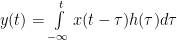 . This becomes
 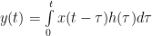 for a causal system if
  for
for  . Equivalently,
 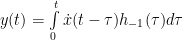 , where
  is the time derivative of
  , and $h_{-1}(t)$ is the step response chosen for the assumed feedback level. Obviously, the conventional result
  does not in general equal the Monckton et al. result
  . (Substitute their
  for
for  and
and  for
for  .) So to me it seemed important, in a “user manual” for the model, to distinguish between the circumstances in which the results would be serviceable and those in which they wouldn’t. And central to this, it seemed to me, was the “transience fraction”
  .
.
Oh, I’m inclined to believe its conclusion that the IPCC’s failure to revise its equilibrium-climate-sensitivity estimates requires explanation. And I do think that parsing a linear system’s step response in the way it does can afford insight. But, although their approach of approximating a convolution with a simple multiplication no doubt has some limited range of applicability, they haven’t bothered to define what that range is. And the authors’ poor performance in defending their paper gives me little reason to take their word on the aspects I don’t independently know.
Over the years I’ve had the misfortune of having to read a great many technical papers, most on subjects I knew little about. When I did so, I rarely had the time to double-check everything, even when I knew how to. But I did look into what I could. If that didn’t check out, it raised my suspicions about the parts I couldn’t investigate.
In this case, Monckton et al. made numerous statements about what the IPCC says and how they use terms. I didn’t go back to determine whether the IPCC said what Monckton et al. said it did and whether they characterized it correctly. What I did do was check the paper for internal consistency and consider Lord Monckton’s subsequent explanations. Neither inspired confidence.
Soon after I initially downloaded the Monckton et al. paper, I put it down in frustration. I was unable to make much sense of, for example, exactly how the subscript
However, many at this site had so gushed over that paper that I eventually resolved to slog through it to the bitter end. It was torture. And my attempts to find guidance in the various discussion threads was of limited help. Most of the responses were either too impressionistic to be of much use or merely directed the questioner to read the paper. So I resorted to writing a post that showed why more specificity was needed about one aspect in particular: that transience fraction
Why
This differs from the conventional linear-systems approach only in that, instead of simply multiplying today’s forcings by a single, time-
Now, to get the convolution
Hence my first post, which was intended to elicit more information about its selection and use. And, in doing so, I treated Monckton et al.’s model as charitably as I could:
Unfortunately, that post did not elicit the information I’d hoped. Still, (between the non-answers, red herrings, and irrelevancies) Lord Monckton apparently did confirm that Monckton et al.’s Table 2 values were based on a step response. I therefore submitted the second post, in which I illustrated that the Monckton et al. approach of simple multiplication instead of convolution can result in large errors.
Eventually, Lord Monckton then attempted to justify the Monckton et al. approach with the following statement:
Now, I have no doubt that there are situations in which the Monckton et al. approach gives reasonable results. But Lord Monckton’s reasoning in this regard does not inspire confidence. It has three problems. values are based on the step response, which is higher for a given climate sensitivity. So Monckton et al.’s approach would infer a lower climate sensitivity than the observed transient climate response warrants.
 to the implausible values for
  to his thinking I has misapplied the notion of feedback when I had actually used it more fundamentally than he to his clear misunderstanding of how the “Bode equation” is applied to electronic circuits to his contention that the Table 2 values make their model nonlinear, Lord Monckton managed to deal incorrectly with almost every issue.
First, Lord Monckton has it exactly backwards. As Fig. 7 of my second post shows, it is precisely in the earlier years that the difference between convolution and Monckton et al.’s simple multiplication by the “pulse” (step) response’s most-recent value is most pronounced (and, incidentally, that the differences among the various feedback levels are hardest to distinguish). Second, although there probably are regimes in which Monckton et al.’s approach could produce a serviceable result, Monckton et al.’s paper doesn’t tell how to distinguish among them; to do that you’d have to do the convolution yourself.
Third, in dismissing “extreme examples,” Lord Monckton was presumably referring to the discussion that accompanied my Fig. 7. That discussion was directed to inferring equilibrium climate sensitivity (“ECS”) from transient climate response, and it showed that the Monckton et al. approach would infer an ECS value close to 3.4 K when the conventional approach infers something more like 12 K.
Was that an extreme example, one to which Monckton et al. never intended their model to be applied? If so, it is curious that §10 of their paper, which they claimed was a “user manual” for their model, characterized it as “narrowly focused on determining the transient and equilibrium responses of global temperature to specified radiative forcings and feedbacks in a simplified fashion.” That doesn’t strike me as the best way to wave the user off from inferring ECS from transient climate response.
Moreover, Lord Monckton misapprehended the nature of the resultant error: “Using a pulse tends to overstate climate sensitivity, for obvious reasons. So if, even using a pulse, we obtain low climate sensitivities, then if we had used a convolution the sensitivity would have been still lower a fortiori.” Again, he got it backwards. Monckton et al.’s
Again, I can’t double check everything in a technical paper; I check what I can. If what I do check doesn’t make sense, I wonder about what I haven’t checked out. In this case the lead author repeatedly got things wrong.
From the red herrings about effective radiation altitude and “Plank parameter”
No, I don’t know about all the conclusions in the Monckton et al. paper; I don’t have all the facts. But the facts I do have do not inspire confidence.
Mr Born is fond of saying I have “got it wrong”. However, on the Planck parameter I have cited Roe’s paper as one that recommends treating the Planck parameter as part of the reference frame of the climate-sensitivity equation rather than as a feedback. Once again, Mr Born uses me as his punchbag when his quarrel is with someone else – in the present instance Gerard Roe.
And once again Lord Monckton mischaracterizes what I said. I was responding to his lecturing me and many others that we had used the “Planck parameter” incorrectly; I never said that he had been doing so. I had no problem with his using it in a forward-block sense as he does, and I never said I did; as far as I can tell that introduces little inaccuracy, at least at the time scales he’s dealing with. My treatment does appeal more to me, and I do believe it’s more correct for time shorter scales, but I was searching for information, not trying to make debating points, so I never raised that that issue, and I don’t now. In this context it doesn’t matter.
In short, I wasn’t saying that either he or Gerard Roe were wrong; I was merely saying that I wasn’t wrong, either. How Lord Monckton sees this as a quarrel with Gerard Roe–and how he similarly sees other aspects of my request for information as quarrels with the IPCC–are obscure.
While it is true that science is a demolition derby in which inadequate hypotheses are knocked to pieces, Mr Born;s attitude here, detected by others than me, has been one of desperately trying to find fault where there is really none to be found, and even of picking nits when there are no nits to be picked. In essence, he objects to our adopting particular values for our transience fraction. As is made plain in the paper and elsewhere, this is a model, so he is free to choose his own transience fractions. We fairly and correctly and in detail stated the basis on which we had derived our approximate values for the transience fraction, explained that they were approximate, and demonstrated by worked examples that the centennial values we had used in our paper were those implicit in the IPCC’s own central estimates of climate sensitivity. He doesn’t like those values. Tough t*tty. Let him debate the matter with the IPCC: his quarrel, here as elsewhere, is with them and not with us. Let him choose his own values. It’s a free country. Not a lot in our paper depends on this, even if he were right. And he’s wrong.
Has he gone through our worked examples using a sub-unity transience fraction, as someone who was genuinely interested in the truth might do? Has he tried to propose values for that fraction as we have applied it centennially to the six RCP scenarios that are markedly different from ours? No. Has he attempted to re-determine centennial sensitivity using his own preferred values rather than ours? No, because he knows perfectly well that he will find himself pinned between our values of the transience fraction and the near-identicalk implicit values in the IPCC’s climate-sensitivity estimates. Here as elsewhere, he has set up an interminable series of petty straw men and then knocked them down. Just read BobG’s comment towards the end of the previous thread on this subject. He called Mr Born’s approach “mean-spirited”.
Mr Born now talks of “red herrings about the effective radiation altitude”: but that was a fundamental error in his own understanding of the science. It was not an error that could be allowed to confuse readers of this blog. And he is plainly insufficiently familiar with the literature to understand that the zero-feedback climate-sensitivity parameter is also known throughout the journals as the instantaneous parameter or the Planck parameter. It needs none of his pejorative quote-marks.
Finally, as Mr Born will by now have realized, this blog requires of its participants a certain minimum of intellectual honesty. Several commenters here have expressed their disappointment that at the end of the previous thread Mr Born accused us of “withholding” information that he had requested when he had not in fact written to any of us to request it, and when the information was in our paper all along, and that he has repeated that allegation by saying at the beginning of the post to which the head posting here is a response that we had “turned down” his requests for that information, which they rightly took to imply that he had actually sent us a request by email and we had refused.
And he has wriggled and quibbled disfiguringly throughout on this point. He wails that Roe’s paper has only one (or maybe three) curves but our table 2 had not one or three but five sets of values. It is plain to anyone looking at Roe’s graph that there are three curves on it. And it is also plain – and explained in the text of our paper – that our fourth set of values – unity where the feedback sum is sufficiently low – is an approximation that will not lead to significant error. As to the fifth set of values, it falls between Roe’s least curve and the very-low-feedback case.
So let us summarize. Mr Born made several errors in his original posting. When we had dealt with those, he decided to have another go, and made further errors, not the least of which was his nasty statement that he had requested us to supply information that we had withheld, and even that we had “turned down” his request, when everything that a reasonable man might have needed to help him understand our approximate values of the transience fraction was in our paper in the first place. Then he spins up some theoretical instances that are nothing to do with any of the worked examples in our paper. Then he relentlessly overlooks our surely reasonable point that this is a model and he is free to choose his own transience fraction values if he wants.
However, he is unable to overlook the fact that the ultimate concern of climate-sensitivity modeling is to determine equilibrium climate sensitivity, and in that circumstance it is a matter of definition that the transience fraction is simply unity. Had there been the slightest doubt about this, our paper makes it explicitly plain.
Finally, Mr Born skates around the fact that at the net-negative feedbacks and consequent very low sensitivities our own model runs suggest the transience fraction will be little different from unity at all points on the time-curve. As BobG has rightly pointed out, Mr Born has made a mountain out of what was not even a molehill, and, in giving the false impression that he had asked us to supply information when he had not in fact got in touch with any of us, and in then failing to apologize, he has lost all credibility not only with us but with many others here.
In the end, the purpose of science is a moral purpose: it is to search for the truth. Mr Born, in departing from the truth by saying we had refused to give him information that he had not contacted any of us to ask for, has demonstrated – to this observer, at any rate – that his interest is not in the truth but in attempting – and, thank Goodness, failing – to divert attention away from our model’s conclusion that climate sensitivity to a doubling of CO2 concentration is very likely to be low.
@Lord Monckton
@Joe Kirklin Born
Gentlemen, thanks for discussing the issues openly. This is, up to now, a pretty unusual thing amongst those who are, at a scientific level, doing “climate research”. I am glad Lord Monckton did not refrain from dealing out his side blows, for which he is notorious for those under the spell of the IPCC and far famed for those who have a more sceptical approach to the matters. Joe born came in -imho- as second winner. As far as I am concerned, I found this discussion very interesting and helpful to me. It shows that platforms like these are absolutely vital to exchange opinions in a civilized manner. I wouldn’t give a sou for that being possible at other places.
“Equilibrium sensitivity is the warming that might be expected to occur by the time the climate had settled back to a steady state in response to a direct forcing followed by the complete action of all temperature feedbacks consequent on that forcing. Now, it is a matter of definition that at equilibrium the transience fraction must in all cases be unity.”
Increased GHG forcing in theory will cause a bias in atmospheric teleconnections that dictate oceanic modes, and hence rates of longer term upper ocean heat content loss or gain. An increase in forcing should increase La Nina conditions, cool the AMO and Arctic, and thereby increase OHC. It’s more like a permanent positive bias on a floating point.
IOW, as regards surface temperatures, oceanic negative feedbacks to an increase in forcing imply TCS to be negative at up to interdecal scales, and only ECS to be positive because of increases in ocean heat content.
Just a note, for many browsers the “clickable link” scibull.com in your article does not resolve. It would seem they do not have an appropriate A record for www . To be helpful to other readers (not that they can’t just type it in) just change the link to point to http://www.scibull.com
As to apologies:
Since I hyperlinked the word “request” to my previous post, which showed why further information about transience fraction was needed, and since I hyperlinked “turned down” to Lord Monckton’s purportedly responsive post, one would have to be transcendently dense to interpret “request” as something other than the post that word was linked to.
Frankly, I don’t think either BobG, who dreamed up that theory, or Lord Monckton, who thereupon seized upon it, seriously believes it. I think that they’re using a willful misinterpretation to imply that I had done something nefarious; they probably thereby intend to divert attention from the substantive issues I raised.
If anyone is owed an apology, it is I.
Joe Born, I can tell you were good at being a lawyer. But you are being deliberately obtuse and deceptive. You wrote, “Lead author Christopher Monckton turned down my request for further information about how the Table 2 “transience fraction” values in Monckton et al., “Why Models Run Hot: Results from an Irreducibly Simple Climate Model,” were obtained from a Gerard Roe paper’s Fig. 6.”
In a blog – how do you know that the person actually read any request you made and if they read them, did they do so before the comments were closed? Answer, you don’t unless you contact them outside the context of the blog.
If I read that someone turns down something, this means that someone requested something and the other party said no. That is why when I read what you wrote, I thought that this must have been what happened. You asked Monckton et. al. for more information about the paper and he said no.
Given what I’ve noticed about Lord Monckton over time, I thought this was extremely odd behavior on his part. Since it seemed so odd, I thought about it further trying to figure out what could have happened. Then I remembered you mentioned you were a retired lawyer and the pieces fell into place.
I think that most of the people on WUWT when they read what you wrote also believed that Monckton et al explicitly turned down a request from you. Nor, do I believe that this meaning was something that a retired lawyer would miss in a million years.
Note, your response is close to exactly what I thought you would write except it didn’t occur to me that you would request an apology. My mistake and I apologize for underestimating you.
The term “feedback sum” is used in many places in the article and comments. When I google for “feedback sum” (in quotes), nothing useful comes up.
What precisely is “feedback sum”?
Monckton of Brenchley: “Mr Born;s attitude here, detected by others than me, has been one of desperately trying to find fault where there is really none to be found.”
Essentially the only innovation in their model outside of its parsing the step response into magnitude and shape factors is its use of simple multiplication in the time domain rather than the more-accurate convolution. And the applications to which they said their model is “narrowly focused” was “determining the transient and equilibrium responses of global temperature to specified
radiative forcings and feedbacks.” So it is hardly a “nit” that when this simple-multiplication approach is used to infer equilibrium response from transient response it confuses a 12 K equilibrium response with a 3.4 K one.
Kevin Kilty has suggested that, despite its avowed focus, the model should not be used for drawing such inferences. As I demonstrated, obviously not. Since the authors contended that their model “allows a rapid but not unreliable determination of climate sensitivity by anyone even at undergraduate level,” though, it hardly seems unreasonable to ask that they inform those undergraduates just what range of applications it actually can be used for.
That would have been a more-constructive response to my last post than to pretend that they have been misled by the way I referred to the previous post.
Mr Born continues to pick nits. Meanwhile, our model is perfectly serviceable and, on the evidence of the download count, a lot of people are using it. The paper is quite explicit that the values in our Table 2 are approximate; it is quite explicit that they are based on a pulse and not, therefore, a convolution; it is quite explicit that the IPCC has its own centennial estimates, which we used (and, as expected, they were not vastly different from the values using a pulse rather than a convolution); and we were quite explicit that people were free to adopt their own parameters. Our paper was written for a scientific audience, and we did not need to teach it to suck eggs by explaining the (in the real world) rather trivial difference between the forcings from a convolution and the forcings from a pulse.
And if Mr Born wants constructive responses in future, then he should a) make serious and substantial points rather than picking nits; and b) not allege, falsely, that we had withheld information that was already available to him, and for which he had not written to any of us to ask. If he had done it once it would have been bad enough, but he did it twice. A far more professional standard is expected in future. He is in no position to pick nits after having behaved as badly as that.
After reading through all this, it is pretty clear that it is Joe Born who has shown bad faith and wriggled around like a typical lawyer. If he doesn’t buy the paper’s results, so be it, nobody cares. All of us who have seen the long draw out posts of his over this whole issue can make up our own minds on who is correct and certainly it is not him.
They’re talking past each other (ie. not even talking the same language). I wouldn’t impute malice to either party.
That is correct, we have made up our own minds about who is correct. It is amusing that for all the criticism about authors of AGW papers not being open and transparent with their data and calculations, when the shoe is on the other foot, the levels of obfuscation are astounding.
In answer to Chris, what data and calculations did we obfuscate or not disclose? Read our paper: everything is explained. Mr Born chose to pretend we had not explained how we derived our values in Table 2: but we did. And, in order for us to have supplied further information, Mr Born would have had to explain what further information he wanted, rather than saying he wanted us to explain what is already quite well explained in the paper, and he would have had to email at least one of us to ask for it.
Chris, your accusation of a lack of openness and transparency is sheer nonsense.
I have never seen any author of a pro CAGW paper, either regarding attrition or causation, so openly discuss on a blog as Christopher Monckton has done here. I have my own thoughts and limitations regarding the technical merits, yet as part of the purpose of the paper is, IMV, an illustration of the models failings, I consider it successful.
In areas of fuzzy persuasion, I learned more from Christopher Monckton’s responses, and I am in good company in crediting the ability of an adept to communicate to lay person constructive understanding, as also being a reflection of the adepts true grasp of cogent material.
In areas and criticisms beyond my capacity, then I must consider the post of Bob G, linked here, quite well stated. http://wattsupwiththat.com/2015/04/05/a-reply-to-born-how-to-represent-temperature-feedbacks-in-a-simple-model/#comment-1899014
If we suddenly had substantial warming, without the water vapor growth, wouldn’t the CAGW hypothesis also be disproved?
Argh, this was meant to be in reply to the water content discussions ….
Assessments using recent data, such as this paper, have produced progressively lower estimates of Climate Sensitivity. Eventually, IMO, Climate Sensitivity will be found to be zero.
Proof has been hiding in plain sight that change to the level of atmospheric carbon dioxide (CO2) does not cause climate change. Only existing data and the relation between physics and math are needed or used. The proof and identification of the two factors that do cause climate change are at http://agwunveiled.blogspot.com .
KevinK
April 5, 2015 at 4:56 pm
“Dear Lord Monckton,
..there is no way that the classical electrical engineer’s feedback equations can be used to predict anything.”
This is too dogmatic a statement for an engineer to make. There are important examples of tools used in one discipline having much broader application than anticipated. When my daughter graduated with a PhD in physics, her first job was as a financial research analyst at the headquarters of a major bank (jobs were scarce at the time). Her boss informed her that equations used in physics have proved to have excellent application in econometric and financial analysis. She was surprised to find the department employed several physicists and mathematicians doing fourier stuff, radioactive decay type stuff, etc.
My favorite (and my climate model) is the Le Chatelier Principle (LCP) which was recognized in the realm of chemistry by its namesake. Essentially it is: that given equilibrium (or really any) conditions a change in temperature, concentration, pressure, volume…..or any perturbation in the system will cause the equilibrium to shift in a direction so as to resist the change (partly). I.e., the direction of change can be predicted from it. Unbeknownst to Le Chatelier, the principle had very broad application across systems. A gyroscope or moving bicycle resists attempts to push it over; stretching a spring, friction…. it is applicable to thermodynamic systems (like climate) – heating invokes mechanisms to cool and vice versa (I believe LCP makes it necessary to invoke entropy of an action). It even has proven useful in exploring price/supply/demand relationships in economics.
Now I don’t know much about feedback in electronic circuits but I dare to say that LCP could be a useful principle to assess what one should expect to happen with increasing gain (an agent will attempt to resist it until overpowered by magnitude). Certainly back EMF in motors is such an idea…..Homeostasis is term that is used in its stead. Newton’s third law (when a body A exerts a force on body B, B exerts and equal an opposite force on body A – when you push against a wall, it pushes back with equal force until you exceed the strength of the wall – the “partly” part of the LCP.
Nature is most economical with its tools and insists on sharing.
A very interesting comment from Gary Pearse on the Le Chatelier principle. The climate has proven near-perfectly thermostatic for the past 810,000 years and – for all we know – longer. Unfortunately, the Bode feedback system gain equation models objects that are very far from homeostatic, which is why we say it should not be applied to the climate – at least, not at high net-positive feedbacks, and not without modification.
Well I’ve been thoroughly entertained by this thread. I’ll not weigh in on either side, I’ll just make an observation and then ask the obvious question, which to my surprise nobody has yet voiced.
Observation: The accuracy of a model can only be ascertained by its ability to predict the future. Hindcasting is of limited value as a correct answer could easily be a consequence of curve fitting. Only by predicting the future, and then seeing what actually happens, can the model be validated. Which brings up two questions, one for Born and one for Monckton:
J Born => For how many years into the future must the model prove accurate for you to admit it is valid?
C Monckton => For how many years into the future must the model prove inaccurate for you to admit it is invalid?
As I understand it – and I am probably wrong, someone has ideas, which he sets out as a theory. He tests this theory by proposing hypotheses which, if the theory is correct, must be true, or, better, if the theory is wrong will be shown to also be wrong. He uses past data to construct a model of his theory, to test one or more hypotheses. He ‘calibrates’ it by using data from the recent past (say, 20 years). He then ‘validates’ it by using data from a previous period, say 100 – 20 bp. If the model works within certain limits he trumpets to the world that his theory is correct. If the results do not pan out, he then shuts up and thinks, was my idea wrong, was my model wrong, is the data wrong (plausible!).
What he rarely does is to go back further, to say 500 – 100 bp, or 2000 – 500 bp. If his data that he used to calibrate the model and the model he constructed are both correct, hindcasting should work equally well back into the dim and distant past. So all these climate models should be able to hindcast the mediaeval warm, the Roman warm, the hypsothermal. If they cannot, they are not worth tuppence.
And if the hindcasting shows they are not worth tuppence, who would expect them to be useful for predicting the future?
That’s not as incisive a question as you may think; there will always be arguments in retrospect about what is meant by “accurate” and what tunable parameters were assumed. So I can’t really answer it.
But I can tell you this. If (1) the Table 2 values (interpolated, say, in accordance with the estimates I set forth in my previous post) do correctly represent the systems’ step responses, (2) CO2 concentration increases 1% per year over the next thirty years without changes in any other forcings, (3) you know what the temperature thirty years from now would be if no forcing change occurred, and (4) you apply the model under the assumption that equilibrium climate sensitivity is 1.4 K and the forcings grow as they turn out to, then the model will “correctly” predict the temperature thirty years from now–but only if the equilibrium climate sensitivity is actually about 3.4 K instead of the 1.4 K you assumed. If the equilibrium climate sensitivity instead actually is the 1.4 K you assumed, your prediction will be 0.1 K too high.
In other words, if you make a prediction for thirty years from now based on the assumption that the equilibrium climate sensitivity is 1.4 K and your prediction comes out right on the money, you will sit fat and happy enjoying your conclusion that you were right to think equilibrium climate sensitivity will be only 1.4 K–even though the real equilibrium climate sensitivity will actually prove to be 3.4 K.
In other words, you can’t conclude much about the model’s accuracy in general from the fact that it gets it right in some interval. That’s why I ignore the conclusions various disputants base on alleged skill; they’re built on sand.
You can prove this all this to yourself by applying the equations and coefficients in my previous post.
Nonsense. The further out in time we go, the more data we have. The more data we have, the more narrowly constrained the tunable parameters become to actual reality. At some point you are left with a sensitivity estimate that is either commensurate with observational data (within some margin of error) or you don’t.
You say the model is wrong. You cannot falsify it by arguing the math. You can only falsify it be setting out conditions in the future that it fails to predict, which you seem loath to do. I can understand that. Jones and Santer probably regret doing the same.
davidmhoffer: “The further out in time we go, the more data we have. The more data we have, the more narrowly constrained the tunable parameters become to actual reality. ” value are that go with it. If you want them constrained adequately during your lifetime or those of your children, though, good luck.
 values exactly right for absolutely every possible equilibrium climate sensitivity value; we don’t have to wait millenia to tune
  . Moreover, let’s assume you can predict the above-mentioned forcings with absolute accuracy and that with absolute accuracy you know what warming is already in the pipeline and what the random variations will be. In other words, give Monckton et al. every possible break.
How much time are you willing to take before you’ve decided you’ve constrained the tunable parameters adequately? Obviously, if forcing changes stop and you wait millenia, then you’ll know what the equilibrium climate sensitivity is and what the
But none of that matters. Because what I’m saying is, Let’s assume Monckton et al. have already gotten the
Even then, the model as they’ve described it will give you an on-the-money prediction only if you assume too low an equilibrium climate sensitivity.
And, yes, that conclusion can indeed be reached by doing the math. I’ve done it, and my previous post tells you how to do it. If you don’t think so, tell me your problem is specifically, and I’ll help. I’m willing to discuss the issues honestly.
If you’re just going to argue, though, I’m not interested.
Joe Born;
If you’re just going to argue, though, I’m not interested.
I’m not arguing, I’m asking a question which you are avoiding answering. Mind you, Christopher hasn’t said a peep, so you get points for at least responding.
Obviously, if forcing changes stop and you wait millenia, then you’ll know what the equilibrium climate sensitivity is and what the r_t value are that go with it. If you want them constrained adequately during your lifetime or those of your children, though, good luck.
First of all, I didn’t say I wanted it within my lifetime or that of my children. I said I wanted to know how long it would take, period. Second, forcing changes don’t have to stop to arrive at conclusions regarding sensitivity and r_t. One only needs enough data regarding what the forcing factors and their changes are for a sufficient period if time compared to temperature over that same period of time to calculate them. I think if the problem was putting a warm beer in a cold fridge and calculating from the temperature changes in the first few minutes what temp the beer would cool to and how long it would take, it would be comparatively easy (for example). But it isn’t and I expect it would take much longer. But it certainly doesn’t have to stop in some steady state to wait for us to calculate the end result.
davidmhoffer: “But it certainly doesn’t have to stop in some steady state and wait for us to calculate the end result.”
In theory, no. In practice, though, if large, slow feedbacks do exist, the difference in the short term between the response without the slow feedbacks and with them is hard to detect.
Suppose you think the step response is 2 / 3.7 * (1 – exp(-t/10)), i.e., the equilibrium climate response is 2 K and there’s no slow feedback. To distinguish that in thirty years from a step response of 2 / 3.7 * (1 – exp(-t/10)) + 2 / 3.7 * (1 – exp(-t/1000)), i.e., from an equilibrium climate response of 4 K with slow feedback, when the carbon-dioxide concentration is increasing at 1% / year, you’d have to resolve a difference of 0.013 K.
@ur momisugly Joe Born April 7, 2015 at 2:25 pm
>>>>>>>>>>
I understand all that. I even agree with all that. But you still haven’t answered the question. How long? 100 years? 1,000? etc?
davidmhoffer: “But you still haven’t answered the question. How long? 100 years? 1,000? etc?” ? Because, as I explained above, we know it will predict too high a near-term temperature change for a given assumed equilibrium climate sensitivity; the math tells us that. And the discrepancy can be significant.
You’re right. And I’m not going to, because that’s outside my area of competence.
By that I mean that I don’t have a clue what the maximum time constants of the system might be, so I couldn’t say how long it should take to be satisfied. I have my suspicions, but they’re probably not worth any more than those of the guy on the next bar stool. Even if a model successfully predicts the temperature thirty years into the future, I still couldn’t conclude that it will be reliable thereafter.
By the way, that is not a comment directed particularly at the Monckton et al. model; it applies to models in general. I just don’t know how I’d tell if they were correctly telling us equilibrium climate sensitivity. And I’m not going to indulge in speculation. I’m sticking to what I can show rigorously.
So why do I have an opinion about the Monckton et al. model’s use of their
But I hasten to add what I think Kevin Kilty’s point above was and what I said in my original post. If you do know what the feedbacks are, I know of no reason why Monckton et al.’s model shouldn’t give you a pretty good idea of equilibrium climate sensitivity. And that means it should be a good way to do a sanity check on whether, say, the IPCC’s equilibrium-climate-sensitivity estimate is consistent with its feedback estimates. I intend to use it in that fashion myself.
Their paper has also served the purpose, I think, of propagating to a greater audience a sense of what significant positive feedbacks’ effects would be if those feedbacks did exist. That is a helpful result.
As to their model’s approach to near-term predictions, though, I wouldn’t use it; it’s internally inconsistent.
So all these climate models should be able to hindcast the mediaeval warm, the Roman warm, the hypsothermal. If they cannot, they are not worth tuppence.
===========
they cannot, because we don’t know what caused them. as strange as it might seem, there is no widely agreed theory of what caused the past warm periods, that appear every 1000-2000 years in the paleo records.
Yet climate science is certain that since they cannot find an explanation for the current warm period either, this warm period must somehow be different and must be caused by CO2.
Sadly, Climate Science continues a long line of bogus, pseudo scientific reasoning, on a par with Eugenics. Popularized by the scientific and political culture of the day in the US, eugenics was adopted by the Europeans with devastating effect. Millions of people were systematically killed to “purify” the Master Race.
Of course, after the war, no one could be found that had supported Eugenics before the War. A legally enforceable Climate Treaty is the obvious precursor to WWIII, as nations will attempt to force other nations to comply, leading to a breakdown of relations as happened in the days and years leading up to WWII.
The ideal solar example of increased forcing is 1970-1976 where La Nina increase, and the AMO and Arctic cool strongly. The cold AMO then increased continental interior rainfall, causing further regional cooling. The corollary of this being the marked decline in the solar signal since the mid 1990’s, with the oceanic negative feedbacks providing a strong AMO and Arctic warming, giving an accelerated global mean surface temperature rise from ~1995-2005, exacerbated by continental interior drying due to the warm AMO mode.
From this frame of reference, TCS to increases in GHG forcing would be a negative bias with regard to mean surface T at least at decadal scales, and only positive with ECS because of increases in upper OHC. So increases in GHG forcing should have reduced warming rates of the AMO and Arctic since 1995. Particularly as there is a near consensus amongst IPCC models that increased GHG forcing will increase positive AO/NAO states, which is the requirement for a cooler AMO and faster trade winds.
http://snag.gy/fjGhc.jpg
Mr Hoffer asks after how many years a model can be said to be invalid. Suppose ad argumentum that the model is by some miracle a perfect representation of reality to date in all respects. It remains a model: in short, the modeler would have to input to it the perfect set of initial conditions in order for it to give a proper output. Now, we have chosen our own set of initial conditions and have run our model using them. We think there will be 0.9 K warming from 2000-2100 caused by Man. We are silent on how much warming or cooling might otherwise occur naturally. So we modelers can get away with almost anything by saying the user had chosen the wrong parameters or Nature had behaved in an unexpected and unforeseeable way.
Perhaps a fairer (and tougher) question, then, is whether over a given period a prediction from one model is appreciably closer to reality than a prediction from other models. One reason why the ClimComms have tried so hard to divert attention away from our paper is that we have gotten into the reviewed literature a really simple new model that (with our choice of initial conditions) predicts lower climate sensitivity than all the general-circulation models. It will gradually become apparent over the century whether we or they are closer to the mark. If we, with our irreducibly simple model, are closer to the mark, governments are going to begin wondering why they paid out all that money for fancy supercomputers, and why they spent $2 trillion and counting as a result of believing the fancy supercomputers, when they could have come to us and, for a mere $20 million or so, we’d have been happy to tell them there will be a little manmade warming, but on balance not very much.
The dispute over the appendices is problematic. Authors should always check the final published work, as last minute edits and snafus happen. In my professional communications (mostly email and wikis), when faced with a misunderstanding such as noted above, I have always double checked to see what the other party is viewing before I assume they are being stubborn. At least half the time the issue was a snafu with an email or other editor. (the other half of the time the other party couldn’t be bothered to read the full missive).
Monckton of Brenchley:
Wow. I had missed that. There it was, the encapsulation of the authors’ lack of candor, their slipperiness, their efforts a plausible deniability: row’s values are unity for all
  , and the wording of §4.8 appears carefully shaded to create the impression those values came from Roe: (“Table 2, derived from [the Roe paper], allows approximate values of
  to be estimated”) but preserve deniability (“Where
  , for all t,
  may safely be taken as unity: at sufficiently small
  , there is little difference between instantaneous and equilibrium response.”). Whether that was the original intent or just another example of the frustrating vagueness that afflicts Lord Monckton’s writing, he thereafter worked to maintain the resultant plausible deniability.
 values were non-physical. On March 1, 2015, for example, Zeke Hausfather said: “There is also the bizarre assertion (via misinterpreting a paper from Gerald Roe) that if feedbacks are negative then the Earth system has no thermal inertia and thus transient and equilibrium sensitivity are the same.” Now, since the
  value was central to the authors’ model, and since Lord Monckton was active on the relevant thread, one might have expected him to address that issue. But Lord Monckton seemed to ignore it.
 had not been. In the face of that representation and the apparent discrepancy, the authors owed their readers an explanation. They needed either to tell how they had derived those values from Roe or admit that they had made them up. Lord Monckton did neither.
 curve, could we really be sure of how they got any of the Table 2 values? Maybe not. The next day I repeated the problem more generally: “The problem I have with using the Roe plot is that Monckton et al. don’t tell how they got from the plot to their table. How, for instance, did they identify the point in that plot’s blue area that represents feedback of 2.1 W/m^2/K at 75 years? . . . Yes, I get it that we can roll our own
  ’s but a reader is justified in wondering how the authors got theirs.”
Lord Monckton still refuses to come out and say what an honest author would have said long ago, as soon as the questions started: Yes, Table 2’s first row was a blunder on our part, and no, we didn’t get the the table’s first two rows from the Roe paper; they’re just our theory: we made them up.
The Moncton et al. paper drew inferences from the fact that the first,
But several people at Climate Etc. pointed out that such
How to get an answer? Well, if our positions had been reversed, Lord Monckton would probably have accused me of falsely alleging that my Table 2’s first row came from the Roe paper. But I’m not lord Monckton
What I did instead was give them the benefit of the doubt and proceed as though the authors had withheld comment about their blunder only because they hadn’t yet grasped the problem. Specifically, I literally drew them a picture. I wrote a March 12, 2015, post in which I laid out with block diagrams and equations just how their transience fraction fit into a linear system. In particular, Fig. 3 depicted the thermal inertia one would expect of a system such as the Earth. I then gently observed that their paper did not made “entirely clear” the manner in which they had obtained the Table 2 values from Roe
On that same day Mr. Hausfather made that point more forcefully on this site by repeating the comment he had made on the other site two weeks before. He then went on to identify the particular equation in the Roe paper that seemed inconsistent with the authors’ contention that they had derived such values from Roe. If I understood him correctly, moreover, he reported a personal communication in which Dr. Roe confirmed that those values were inconsistent with his paper.
Now, in that situation, wouldn’t candid authors just say, Sure our values are inconsistent with the Roe paper; they’re our own theory, we made them up? Of course they would. But that’s not what Lord Monckton did.
Two days after those values’ provenance had thus been called into question for the third time, Lord Monckton finally issued a comment. But instead of coming clean, he gave a non-response: he again withheld how those values could have come from Roe. (All four authors object to my using “withheld” for this situation. What would they prefer, “divulge”?) He merely stated that Monckton et al. were right and Mr. Hausfather was wrong. (Oh, and he muddied the waters further by adding that “the transience fraction exceeds unity where feedbacks are net-negative,” but I assume he has since quietly repented of that notion.)
So the next day I provided Lord Monckton yet another way of looking at Monckton et al.’s error. In a comment in response to Lord Monckton’s, I suggested that he make a plot like what would ultimately be my subsequent post’s Fig. 1. That would have made apparent how anomalous those values are: they make a higher transient response lead to a lower equilibrium response.
In short, Lord Monckton had been informed (1) that those Table 2 values ignored thermal inertia, (2) that they associated a higher transient response with a lower equilibrium response, and, apparently, (3) that Roe said such values were inconsistent with his paper. But in Lord Monckton’s next communication, a new head post, he merely repeated that the values came from a graph in that paper: “The table was derived from a graph in Gerard Roe’s magisterial paper of 2009 on feedbacks and the climate.” Instead of admitting what happened, he engaged in more misdirection: “If Mr Born disagrees with Dr Roe’s curve, he is of course entirely free to substitute his own.” Of course, the curve at the heart of my objection was not Dr. Roe’s at all; it was one the authors had made out of whole cloth.
Now, despite all the back and forth, the discussion so far had boiled down to the following. Monckton et al.: “We got those values from Roe.” Born: “I don’t see how you could have gotten them all from Roe.” Monckton: “We got them from Roe.” Lord Monckton likes to characterize this as my never having asked how they got the Table 2 values. Well, if I wasn’t asking for them, it was in the same way that it isn’t asking for your change to tell the cashier, Hey, I didn’t get my change: Lord Monckton’s playing word games. And, no, Lord Monckton did not say, “I’m going to turn down your request that we tell how we got those values from Roe.” But turn it down he did, and that’s how I later, correctly, characterized his post.
My first comment on the ensuing thread made it as easy as possible to see the anomaly: I gave actual code that could simply be plugged into an R interpreter to graph the step responses Moncton et al.’s Table 2 implied and thereby see how it anomalously associates higher transient responses with lower equilibrium climate responses. That occurred on March 16, 2015, the day of Lord Monckton’s post. From the resultant plot anyone who understood the subject matter could tell at a glance that the Monckton et al. had blundered.
In response Lord Monckton again stonewalled: “As to the values of the transience fraction over time, Mr Born is free to adopt any values he wishes.” Of course I was. That wasn’t the issue. The issue was that Monckton et al. had represented the Table 2 values as having been derived from Roe, and there was every indication, including apparently the opinion of Dr. Roe, that at least those for
If he wasn’t coming clean about the
Then silence.
Oh, Lord Monckton submitted numerous comments on that thread, but for a full week none was no satisfactory reply. Nothing. I then submitted a five-comment wrap-up that ended with an expression of my disappointment that Lord Monckton had insisted on withholding information about how Monckton et al. had inferred the Table 2 values from the Gerard Roe paper.
It turns out that comments on that thread were thereafter closed, and the authors seized upon that fact as their excuse for not having provided the requested information—even though the issue had been raised repeatedly during the previous weeks and Lord Monckton had stiff-armed us on each occasion.
On April 1, 2015, I submitted a second post. As I said, I had previously described how to graph the values to see how implausible they were. Then I had supplied turn-key code to enable the authors to generate a graph that would illustrate it. In that second post, I provided the graph itself as Fig. 1.
The first sentence of that post included the word “request” hyperlinked to my previous post and thereby describing it as a request for further information about how the Table 2 values were obtained from Roe. The words “turned down” were hyperlinked to Lord Monckton’s post, thereby saying that I considered that post to turn down my request. To anyone familiar with hyperlinks, that leaves left no question that by “request” I was referring to my previous post. Yet Lord Monckton’s apologists profess to have interpreted that as saying the request was not in a post but in a separate communication.
And in Lord Monckton agreed: “Mr Born did not explicitly ask how we determined our approximate values for the transience [fraction] until so late in the day – and in a startlingly discourteous fashion – that I could not have commented even if I had wanted to. Comments had for some reason been closed on that thread.” Note the wordsmithing. Saying you didn’t get your change is not “explicitly” asking for the change. Note the false excuse. Comments had been closed only after the issue had been raised weeks before in several different ways. And note the ginned-up outrage. To Lord Monckton it’s discourteous to state plainly what has been going on: Lord Monckton had withheld the information.
And then the disillusioning part. In the head post here, Lord Monckton’s co-authors became complicit:
This time they didn’t repeat the statement that the Table 2 value came from Roe, but neither did they clearly say the table’s first two rows hadn’t: plausible deniability.
Although I had attempted without success to obtain an explanation at author Briggs’ site, I had entertained the notion that the stonewalling was just Lord Monckton, that if faced with the issue the other authors would come clean. I was saddened to see them join in such shabby behavior. If they had been candid, they would have taken the opportunity to come right out and said it: Those first two rows didn’t come from Roe, the authors made them up, and the fact that their implied step responses intersect shows that they thereby made a mistake. But they didn’t.
How disappointing.
Why not write your own paper with your own colleagues then, instead of this weasel worded attack on others. You imply many things about Dr. Roe and yet YOU have provided NO evidence that you have even corresponded or spoken to Dr. Roe on this matter, nor have we seen complaints from him.
You are a serial mudslinger Mr. Born, an agent provocateur, and a nit picking troublemaker.
FACT ….. and you know it.