By Andy May
Frank Stefani, of the Helmholtz-Zentrum Dresden-Rossendorf, Institute of Fluid Dynamics, has published a very interesting new paper that compares the solar “aa” index and CO2 emissions to global SST (sea surface temperatures using the HadSST4.2 dataset) and finds a CO2 sensitivity (TCR or the “Transient Climate Response”) of 1.1 to 1.4K. This is at the low end of the IPCC TCR range of 1.2 to 2.4K (IPCC, 2021, p. 93), but quite close to the values calculated by Lewis and Curry and Nicola Scafetta (Lewis & Curry, 2018), (Scafetta, 2023), and (Lewis, 2023). Scafetta found a plausible range of TCR (versus HadSST4.2) of 1.0K to 1.2K and Lewis & Curry report a range of 0.9K to 1.7K for TCR versus HadCRUT4. The estimates are compared in Table 1.
Table 1. Estimates of TCR, or Transient Climate Response to a doubling of CO2. Sources: (Stefani, 2026), (Lewis & Curry, 2018), (Scafetta, 2023), and (IPCC, 2021, p. 93).
TCR Estimates | ||||
Author | Best Estimate | Range: Low end | Range: High end | Note |
Stefani | 1.26K | 1.1 | 1.4 | 2026 |
Lewis & Curry | 1.2K | 0.9 | 1.7 | 2018 |
Scafetta | 1.1K | 1 | 1.2 | 2023 |
IPCC AR6 | 1.8K | 1.2 | 2.4 | p. 93 |
All the estimates in table 1 are based on regression models of varying complexity and all attempt to account for the influence of solar variability. The Lewis and Curry estimate does not incorporate a solar activity proxy directly but does use the Atlantic Multidecadal Oscillation (AMO) as an indicator of natural climate variability, which is, in large part, solar variability. Stefani uses the aa index of geomagnetic activity, essentially how disturbed Earth’s magnetic field is by the sun. It is measured in nanoteslas (nT).
Nearly every observable form of solar variability is a magnetic phenomenon at its core, including sunspots, flares, and solar wind variability. Thus, the aa index is a good indicator of changes in the sun’s state and output. The aa index as a measure of solar-geomagnetic coupling has been measured consistently since 1868.
Table 1 shows that Stefani’s aa index + CO2 model compares well to Lewis and Curry’s AMO + CO2 model and Scafetta’s solar proxies + CO2 model. Scafetta uses three estimates of total solar irradiance (TSI) in his study, although he acknowledges that variations in TSI may be only ~20% of the sun’s total influence on Earth’s climate. None of these observation-based models support the high-end IPCC TCR estimate of 2.4K per doubling of CO2 or their best estimate of 1.8K, but all are near the lower end of the IPCC range. The Lewis (2023) correction to the Sherwood (2020) assessment of ECS and TCR relied upon in AR6 is not included in the table. However, after changing Sherwood’s subjective Bayesian assessment of multiple estimates of TCR to an objective Bayesian assessment, Lewis calculated a TCR of 1.37 to 1.4 depending upon the assumptions made. This is still close to the other observation-based objective estimates in Table 1.
Stefani found that the solar aa index can successfully predict HadSST4.2 up to 1990-2000 on its own. After 1990 to 2000 the role of CO2 in the regression increases significantly. In figure 1, Stefani’s robust aa index weight of 0.04 K/nT (that is the HadSST4.2 anomaly temperature in °C per the aa index in nanoteslas) plus CO2 with a sensitivity of 1.26K per doubling is shown as a thin dark gray line. It is compared to the HadSST4.2 anomaly (shown as black dots). His projected aa index plus CO2 at 1.26K per doubling function to 2100 is shown as a red line. The maximum departure in 2023 and 2024 looks startling, but we need to remember that this follows two strong El Niños (2018-19 & 2023-24) and the Hunga Tonga volcanic eruption. In particular the El Niño from June 2023 to May 2024 was one of the strongest El Niños on record. The HadSST4.2 global anomaly has been falling since September 2024. Thus, a portion of the difference between the aa index plus CO2 function and HadSST4.2 may just be ENSO, the Hunga Tonga eruption, and weather.

Stefani’s optimal model projection to 2100 assumes constant emissions of 30-50 Gt of CO2 per year (roughly current levels) plus a simple linear carbon sink model and predicts a global SST increase of 0.6°C (1.1°F) compared to the standard HadSST4.2 reference period of 1961-1990. Using pessimistic parameters (high CO2 emissions, a low sensitivity to the aa-index, and a high sensitivity to CO2) yields a 2100 temperature increase of ~1K over 1960-1990. This is still a benign result.
A word on Transient Climate Response
The transient climate response is the modeled warming due to increasing the atmospheric CO2 concentration by 1% each year until it doubles, which would take about 70 years. This is different from the commonly cited value of ECS, which is the equilibrium climate sensitivity, or the final warming due to a sudden doubling of CO2. ECS is an untestable number, since it would take over 1,000 years for the atmosphere to completely come to equilibrium after CO2 suddenly doubles. Given the implausible scenario, ECS can never be tested, except in a climate model. Thus, it is not a scientific quantity per Karl Popper (Popper, 1962). TCR on the other hand is very realistic and could be tested given enough time and effort.
Conclusions
The paper is a welcome addition to the growing group of observation-based estimates of climate sensitivity to CO2. It is appropriate that Stefani chose to create his model around HadSST4.2. SSTs are more stable than air temperatures on land and they respond mainly to changes in insolation, whether due to cloud cover changes or changes in the sun itself. The changes in SST due to the greenhouse effect are smaller for the reasons discussed in my previous post. I recommend the paper, it is interesting, significant, and a good read.
Works Cited
IPCC. (2021). Climate Change 2021: The Physical Science Basis. In V. Masson-Delmotte, P. Zhai, A. Pirani, S. L. Connors, C. Péan, S. Berger, . . . B. Zhou (Ed.)., WG1. Retrieved from https://www.ipcc.ch/report/ar6/wg1/
Lewis, N. (2023, May). Objectively combining climate sensitivity evidence. Climate Dynamics, 60, 3139-3165. https://doi.org/10.1007/s00382-022-06468-x
Lewis, N., & Curry, J. (2018). The Impact of Recent Forcing and Ocean Heat Uptake Data on Estimates of Climate Sensitivity. Journal of Climate, 31, 6051-6071. DOI: https://doi.org/10.1175/JCLI-D-17-0667.1.
Popper, K. R. (1962). Conjectures and Refutations, The Growth of Scientific Knowledge. New York: Basic Books. Retrieved from http://ninthstreetcenter.org/Popper.pdf
Scafetta, N. (2023). Empirical assessment of the role of the Sun in climate change using balanced multi-proxy solar records. Geoscience Frontiers, 14(6). Retrieved from https://www.sciencedirect.com/science/article/pii/S1674987123001172
Sherwood, S. C., Webb, M. J., Annan, J. D., Armour, K. C., J., P. M., Hargreaves, C., . . . Knutti, R. (2020, July 22). An Assessment of Earth’s Climate Sensitivity Using Multiple Lines of Evidence. Reviews of Geophysics, 58. https://doi.org/https://doi.org/10.1029/2019RG000678
Stefani, F. (2026). Solar and Anthropogenic Climate Drivers: An Updated Regression Model and Refined Forecast. Atmosphere, 17(3). https://doi.org/10.3390/atmos17030252
Hindcasting for fun and profit.
Andy,
The most obvious failing of your comparison is that whatever sensitivity Stefani has calculated, it is for SST, not air temperatures. Most of the indices you have calculated it for air for air temperatures.
But he hasn’t calculated TCR at all. There is no attempt to look at an increase of 1% pre year over 70 yers, as you explain. All he has is a regression coefficient.
And it isn’t a proper regression coefficient, as he rather remarkably admits:
” Although this procedure may appear to be a “statistical sin”, I consider its outcome to be better justified than that of a “correct”, albeit somewhat naive double regression. That way, the CO 2 sensitivity was narrowed down from the ample range of 0.6–1.6 K derived in [ 39 ] to 1.1–1.4 K. The alternative double regression would not only have resulted in a moderately enhanced CO 2 sensitivity value of 1.74 K, but also in a dramatically reduced aa sensitivity of 0.011 K/nT. Faced with the choice of either accepting an unreasonably huge reduction in the aa sensitivity over the last two decades (compared with its stable long-term average) or attributing some of the recent steep warming to factors other than CO2 or the sun, I opted for the latter.“
Weird. It is a sin. He knows how it should be done (double regression), but that gave too high a result (1.74). So he rejected that because he thought it too high, and hacked together a home made procedure which gave a result he liked better.
And Nicky knows about “statistical sin”. 😉
All true, but I did not consider it a failing.
First, the distinction between SST and air temperatures is valid, but it’s not a showstopper here. Stefani’s focus on SST aligns with how ocean heat content drives much of the climate system—air temps often lag or amplify SST changes. Many sensitivity estimates (e.g., from ARGO data or satellite records) use SST as a proxy because it’s more directly measurable over long periods. If anything, this makes his approach conservative, as SST warming tends to be slower than surface air temps in most datasets like HadCRUT or GISS.
He estimated TCR, while including a proxy for the sun’s effect on Earth’s climate. The aa index is arguably a better proxy than TSI (total solar irradiance) for the effect because all or nearly all the changes in the sun are related to changes in its magnetic field. TSI is a side effect, not the cause. The aa index (geomagnetic activity) is indeed a stronger correlate for solar influence than TSI alone, as it captures magnetic field variations that affect cosmic rays, cloud formation, and potentially albedo—mechanisms TSI misses. Studies like those from Svensmark or Shaviv support this; TSI is more of a byproduct of magnetic cycles, not the primary driver.
Statistically what Stefani did was a sin, but how many sins statistical have the consensus committed? I couldn’t even count them. I mention Sherwood in the post as an example. Climate science is riddled with similar adjustments. Sherwood et al. (2020) on hot spot amplification relied on reanalysis tweaks that inflated sensitivities, and AR6’s narrowing of ECS (1.5–4.5 K) involved downweighting high-end models post-hoc. Or take Mann’s hockey stick—principal component centering was a “sin” that exaggerated recent warming. If we’re calling out sins, consistency demands we apply it across the board, given you are part of the consensus you don’t want to go there.
Both ECS and TCR are model fantasies. Useful heuristics, but they’re model-derived abstractions that assume CO2 dominance and linear forcings. They ignore nonlinear feedbacks like solar-ocean coupling or multidecadal oscillations (AMO/PDO). Real-world CO2 growth isn’t exactly 1% per year, but from ~280 ppm in 1850 to 425 ppm today is about 52% total increase over 176 years (using NOAA data), averaging ~0.3% per year. Over the last 50 years (1974–2024), it’s closer to 0.5–0.6% annually. Stefani, Lewis, and Scafetta all work in this observational ballpark, yielding lower sensitivities (1–2 K) that better match the ~1.1°C warming since 1850 without invoking massive positive feedbacks. If solar forcing via aa explains even 20–30% of that, CO2’s role shrinks accordingly.
That is Stefani’s very valid point.
Andy,
On your first point, you say it yourself:
” SST warming tends to be slower than surface air temps in most datasets like HadCRUT or GISS”
Yes, and so Stefani’s SST “sensitivity” would necessarily be less than an air sensitivity. The IPCC would have quoted lower numbers for SST.
Second point: you listed the requirements for TCR. They are specific – 1% per year, 70years. They appear nowhere in Stefani’s calculation.
Your third is the typical WUWT defence of last resort. OK, our paper is rubbish, but what about Mann, or Sherwood, or whatever? The relevant point is that our paper is rubbish.
“surface air temps”
This is typical climate science cognitive dissonance. We live *on* the surface, not in the air. Soil temperatures are more of a major factor in climate than air temperature six feet above the soil. That’s not to say they are not related but it is a complicated functional relationship and not the simplistic assumption that air temperature is surface temperature.
This is why it was agriculture science found the increase in growing seasons, not climate science. It was agricultural science that forecasted larger food production because of this, not climate science. Climate science has, and still does, predict LOWER food production from higher air temperatures. It was remote sensing science that first found the “greening” of the earth, not climate science. Climate science only predicted *less* green as higher temperatures destroyed plant life.
Freeman Dyson’s main criticism of climate science, and especially the climate models, was that climate science is not holistic and it requires a holistic approach to classify climate and its impacts.
The truly sad fact is that even after 50 years of intense study, climate science can’t even accurately predict the air temperature anywhere let alone globally. That’s not likely to change unless climate science moves away from using simplified “averages” that are inaccurate and moves toward developing holistic algorithms for the biosphere.
“This is typical climate science cognitive dissonance. We live *on* the surface, not in the air.”
But we don’t live in the sea.
“Soil temperatures are more of a major factor in climate than air temperature six feet above the soil.”
SST is sea surface temperature, not soil temperature.
70% of the Earth’s surface is covered by water.
And what percentage of people live in that 70%?
What percentage of people depend on harvests extracted from the sea?
Not relevant.
“Not relevant.”
It is if you are claiming we live there.
Nailed it!
But much of what we harvest from the sea DOES live in the sea, just like much of our land harvests live in the soil!
And I know what SST is. But as usual you don’t don’t seem to understand the REAL world significance.
Typical deflection. Why can you just not admit you misunderstood what SST means?
You said it was more important to measure soil temperature than air temperature because we don;t live in the air. Now you switch to talking about fishing. Of course 100% of what we harvest from the sea comes from the sea, just as 100% of what we harvest from the land comes from the land. It’s got nothing to do with comparing sea temperature with global temperature.
It sure does have something to do with global temperature.
Attribution for one. There are three pieces being dealt with, atmosphere, land, and ocean. Averaging them without appropriate weighting is incorrect.
Land and ocean are heat sinks. They “store” some amount of heat for a period of time that is not available for heating the atmosphere. If that storage amount and storage time is different in land and ocean, the air temperatures will not be comparable. (Not that they are anyway due to enthalpy.)
Land insolation peaks about noon local time, yet air Tmax doesn’t peak until 2 – 3 hours later. Why is that?
What has any of this got to do eith tge comment I was responding to? It’s just the usual Gorman distraction technique.
“What has any of this got to do eith tge comment I was responding to? It’s just the usual Gorman distraction technique.”
In other words, “I have no answer”.
It has to do with your comment, not the one you were responding to. I even quoted you as follows.
Answer the question I asked.
“It has to do with your comment”
Then address that comment. Why do you think it’s appropriate to ignore the 30% of the globe that is land in order to determine the global TCR?
“Land insolation peaks about noon local time, yet air Tmax doesn’t peak until 2 – 3 hours later. Why is that?”
If you don’t know, why not just do an internet search. But it should be pretty obvious that heat builds during the day. That even as solar radiation decreases after noon, the air is getting more radiation then it is emitting. I’m really not sure why this confuses you.
But again, all of this is a distraction from the claim that we should ignore land temperatures.
No sh*t, Sherlock.
Why is the question! What are the intermediate processes that are occurring? Can these processes be the cause of the radiation imbalance? Why does climate science try to connect insolation diectly to air temperature?
The point is that soil and water are heat sinks but they are never treated as such. They are treated like black bodies, what comes in immediately goes out.
You’ll never get an answer to this from bellman. He has absolutely no knowledge of the real world – including thermal inertia.
“ Why do you think it’s appropriate to ignore the 30% of the globe that is land in order to determine the global TCR?”
As Andy has already pointed out, TCR is a non-physical product determined from a model, not from measurements. A model can ignore whatever the modeler wants to ignore.
” But it should be pretty obvious that heat builds during the day.”
That is *NOT* an answer as to why heat builds during the day instead of changing instantaneously.
“That even as solar radiation decreases after noon, the air is getting more radiation then it is emitting.”
What determines the amount of heat the surface is emitting? Go look up the term “thermal inertia”. And what determines the amount of heat the “air” is emitting? Again, look up the term “thermal inertia”.
This is all part of why it is inappropriate to classify the Earth as a black body with an emissivity when determining instantaneous radiation flux balance.
“But again, all of this is a distraction from the claim that we should ignore land temperatures.”
Determining how the oceans react is *NOT* ignoring land temperatures. You are still showing your lack of reading comprehension skills.
” A model can ignore whatever the modeler wants to ignore. ”
Not if you are claiming that TCR is less just because you’ve ingored the faster warming parts if the Earth. That’s like removing the fastest raising prices from your inflation calculation and then claiming you’ve reduced inflation.
“That is *NOT* an answer as to why heat builds during the day instead of changing instantaneously. ”
It’s not a question of it changing instantaniosly. It’s the fact that the temperature doesn’t instantly rise to a point where energy out equals energy in. Until it reaches that point the temperature will continue to rise even as energy in decreases. As I say, if you really don’t understand this I’m sure there
are sources on the web that can explain it better than I can.
“What determines the amount of heat the surface is emitting?”
Its temperature.
“Go look up the term “thermal inertia”.”
See, you do understand it. But that’s just a phrase for what I’m trying to explain. It takes time for a body to reach the equalibrium temperature.
“Determining how the oceans react is *NOT* ignoring land temperatures.”
It’s what you’ve been arguing whever you understand it or not. You said at the start the model van ignore anything you want. In this case, by only using SST the modeller is ignoring land.
You can’t seem to get it into your head that TCR is derived FROM A MODEL!
Are you *really* trying to say that the model has included *ALL* physical factors?
The question you were asked is WHY IS THAT? Not “what is happening”. You were told what is happening.
It’s not due to energy in and energy out, at least not totally. It’s mostly due to the thermal inertia of the surface material, be it water or soil. The specific heat and thermal heat conductivity are crucial in understanding surface and sub-surface physical processes for both land and water.
The TCR estimate is done for “over water”. You are doing nothing but whining that Stefani didn’t find a composite TCR for the land/water combination. You can’t find the composite until you find each component.
Stop whining.
Again, you have *NO* understanding of physical processes. Your grasp of reality is tenuous at best. You didn’t bother to go look up “thermal inertia” at all, did you?
If you pulse heat into the heat sink on a computer main processor (perhaps from hitting the spreadsheet calculate key), the temperature of that heat sink will continue to rise for a period of time EVEN AFTER THE PULSE HAS ENDED. That process has nothing to do with energy in equaling energy out at any point in time. It has to do with the thermal inertia of the heat sink.
This basically all boils down to the fact that you, as well as climate science, tries to equate temperature with heat (joules). THEY ARE NOT THE SAME THING. 10 joules in for one second will equal 1 joule out for 10 seconds as far as heat is concerned – and the temperature of the object being heated is not dependent on the temperature of the object doing the heating. Since the earth radiates heat 24 hours per day while the sun only inputs heat for about half that period of time, the temperature of the earth doesn’t have to rise to maximum based on the energy being input. If it did the earth would become a frozen ball at night!
And it’s not just this either. If the energy in equals the energy out and together they determine the temperature of the earth then how does AGW happen?
You don’t understand it at all! Equilibrium with what? Again, as a heat sink and not a black body, the maximum temperature of the earth is not driven by the instantaneous energy input. The temperature of that heat sink will be determined by its thermal inertia. Objects with high thermal inertia heat up and cool down slowly, their temperature tends to be more stable than objects with low thermal inertia. Water, sandy soil, loam, rock, etc all have varying specific heat capacities and thermal conductivities – meaning that they all reach different maximum temperatures from a specific heat input because of their thermal inertia.
“It’s what you’ve been arguing whever you understand it or not. You said at the start the model van ignore anything you want. In this case, by only using SST the modeller is ignoring land.”
SO WHAT? Again, you have to understand the components before you can understand the composite of the components. You are just whining that someone is working with a component instead of the composite. Again, SO WHAT?
Again, you have to understand the components before you can understand the composite of the components.
Here is what CoPilot gives after summarizing several published studies..
Your “lag” is basically the system’s thermal inertia showing up: some of the net radiation is going into soil heat storage (via (G)), so the surface and near‑surface air don’t warm instantaneously with insolation.
Flux is time dependent. You can’t just add them as if they represent an energy value. To actually find the energy balance you need to integrate each term and then add them. Which, in turn, means you have to know the functional relationship to time for each component.
I’m not sure it is wise to take advice concerning what you can and can’t do with radiant exitance fluxes (in W.m-2) from a guy who vigorously defends the notion that they are extensive properties.
You have no room to criticize. If you can’t show that fluxes need to be normal to a point, then you can’t prove they are additive. This is difficult to do with what is absorbed on a sphere. Similarly, the fundamental units are (Joules/sec·m²). S/B is not a panacea for determining the heat from a flux unless you are dealing with a black body.
Q = mcₚΔT is the definition of heat. Or ΔT = Q / mcₚ. Note the use of ΔT. Heat is defined by the difference in temperature. It is not an equation that you can use to determine a temperature unless you already know the heat that has been added. Q’s units is Joules. That is, total Joules needed to cause rise in temperature. In other words, an integrated flux over time.
Don’t confuse the earth with a black body, it is not. Ideal theory is an important place to start but one needs to move into the real world at some point. Read Planck about a pure reflection of radiation from a body. See what he says about how those fluxes add to make the body warmer. Show the math that refutes that.
Read Planck’s Heat Treatise and his lectures to Columbia University. Entropy is a real bitch. I can’t beat it, you can’t beat it, up to this point, no one has ever beaten it or we would have perpetual motion machines. Cold will never warm hot. I don’t care how much flux you add together.
Of course I have room to criticize. Radiant exitance fluxes (W.m-2) are intensive properties because they don’t depend on the size of the system. If you have a 1 m^2 surface emitting homogenously then the right half will have the same radiant exitance as the left half and of the whole. That’s what makes it intensive. You can mock me all you want. It’s still an intensive property.
You’re not going to see me adding radiant exitance fluxes that’s for sure.
“…Stefani didn’t find a composite TCR for the land/water combination.”
That’s the problem. The TCR is not the temperature just over water. It’s defined in relation to the globally averaged surface temperature. You can’t just ignore temperature change over 30% of the globe and say you have determined the TCR. You can derive an estimate for how much changes there will be in sea surface temperature – but that is not the TCR. And whatever you call it you cannot do what May does, and say it’s at the low end of the IPCC TCR range, becasue you are comparing two different things.
A completely nonsense, unmeasurable quantity.
Bellman *still* thinks that an average of measurements is a measurement as well.
Yep. As you keep pointing out, he has no experience in the real world.
The GUM says it is. For example see [JCGM GUM-6:2020] section 5.7 and E.2.2 for explicit statements that measurands can be averages.
And of course the GUM has many references and examples of averaging. Section 11.10.4 even discusses a measurement model that is an average of other measurement models.
Granted…the GUM does contain examples of averaging intensive properties (including temperature) which you vehemently reject so I have my doubts whether you will be persuaded but it is worth a shot.
Do you have a clue about fitness of purpose? Let’s look at [JCGM GUM-6:2020] Section 5.7
The conformity assessment can encompass an average mass of a batch of objects. It is used to check the dispersion of a manufacturing process, not to determine a single measurand. Think tolerance. Think quality control.
Here is what ANSI has for a definition. StandardsAlliance-Handbook-2022-SECTION5.pdf
What is conformity assessment? Conformity assessment is the term given to techniques and activities that ensure a product, process, service, management system, person or organization fulfils specified requirements.
It has nothing to do with averaging measurements to determine a single measurand.
Now let’s look at your E.2.2 reference.
As usual, you miss entirely the need for measuring the SAME THING. This is not measuring 5 different strings and averaging the values to get one measurand. It is measuring ONE string at five points approximately equally
spaced along its length using a caliper.
Lastly, maybe you read 5.6 also. What it says is important.
5.6 When building a measurement model that is fit for purpose, all effects known to affect the measurement result should be considered. The omission of a contribution can lead to an unrealistically small uncertainty associated with a value of the measurand [156], and even to a wrong value of the measurand. Considerations when building a measurement model are given in 9.3. Also see JCGM 100:2008, 3.4.
See that [156] reference. It goes to THOMPSON, M., AND ELLISON, S. L. R. Dark uncertainty. Accred. Qual. Assur. 16 (2011), 483–487.
Here is the abstract from the paper.
Reproducibility deviation is an item on an uncertainty budget. Read JCGM 100-2008; B.2.16, F.1.1.2, and H.6.
Now read NIST TN 1900 EX. 2 and see if this applies when measurement uncertainty is negligible and the difference among samples is used to calculate the repeatability uncertainty.
There are online classes in metrology that you can take. I suggest you do so.
Nothing in your post invalidates the GUM’s statement that a measurand can be an average of something.
Great response, but it is wrong. Maybe you have difficulty in understanding what I posted.
Read this again.
These two parts of conformity testing go together. The mean and the dispersion around that mean. Look up what six sigma means in terms of quality control.
You can’t simply ignore that that the purpose of averaging a batch of objects to determine if the average of a batch of objects is within a specified limit is a legitimate purpose of quality control. You also can’t ignore that the dispersion (standard deviation) of that batch is important also.
It unequivocally says a measurand can be an average mass of a batch of objects.
This is why it is so difficult having a conversation with you. Bellman or I will point out that the GUM, NIST, etc says A. You then cite B from the same source and insinuate that it invalidates A..
I don’t even know why you even bother citing the GUM, NIST, etc. anyway since they have examples of averaging intensive properties which you vehemently reject as being meaningful and useful.
Global average air temperatures are a meaningless statistic that cannot represent “the climate”.
Cue the usual “buh, buh, but WUWT publishes them!”
Neither bdgwx or bellman seem to be able to differentiate between
You *can* measure the temperature of a single object multiple times and average the readings to get a “best estimate” of the temperature (an intensive property) for that single measurand.
You can *NOT* measure the temperature of multiple objects and average the readings to get a “best estimate” of the intensive property of the multiple objects.
You can only get a physical average for a property you can add physically. E.g. mass. You can *not* get a physical average for a property you can’t add physically.
1g + 1g = 2g
80F + 70F ≠ 150F
Statisticians and computer programmers think you can average anything and get a physically meaningful value. Engineers and physical scientists know that the *real* world doesn’t work that way.
“Neither bdgwx or bellman seem to be able to differentiate between
This differentiation has been put in front of them innumerable times, and they invariably avoid the inconvenience. At this point I have to acknowledge the possibility they do understand the difference but are forced to ignore it to keep the fiction of climatology trendology alive.
A Type A uncertainty evaluation is done on each input quantity separately and then combined. Each input quantity has multiple single observations of the same thing that are considered entries in a random variable. The mean and standard deviation of the random variable make up the estimates of that input quantity.
You can declare a monthly average as your measurand and use daily temps as the observations. However a Type A evaluation requires those observations to form a random variable X1 (one input quantity) of which the mean and standard deviation are the estimates of the measurand. Inherent in this is the need for the functional relationship to have only one variable. That is, f(x) = (X1).
Each data point has uncertainty that contributess to the combined uncertainty AND the dispersion of the values must also be added to the combined uncertainty.
This what NIST TN 1900 does. They declare the measurement uncertainty of each observation to be negligible and then calculate the dispersion of the values.
I do have a problem with using an expanded SDOM rather than the SD. However, ±1.8°C versus ±4.1°C are both reasonable.
“Neither bdgwx or bellman seem to be able to differentiate between…”
Stop lying. I’m sure I’ve been over the difference with you multiple times. It doesn’t alter the fact that an average if multiple measurements of the same thing and the average of multiple different yhings are both useful and can both be considered measurements if you wish.
You just need to be clear what the measurand is. In the first case it’s the specific quantitu you are measuring and i. the sevond it’s the mean of the population you are sampling.
“You *can* measure the temperature of a single object multiple times and average the readings to get a “best estimate” of the temperature (an intensive property) for that single measurand.”
Of course you can, but your entire logic of not averaging intensive properties was this it would be meaningless. In both cases you have to add up intensive properties, which is meaningles. If I measure a rock 20 tomes and get a sum of 400°C, what does that temperature mean, and how would be different if I added the temperature of 20 different rocks and got the same 400°C? You either have to accept that having a meaningless part of an equation dors not necesserily invalidate the final result, or you need to cone up with a different excuse for not wanting to consider average temperatures.
“You can only get a physical average for a property you can add physically. E.g. mass.”
As I keep trying to explain, averaging a sample is just a way of estimating a population mean, and in the case of an intensive property the population mean is really the mean if some implicit extensive proprty. If you want the average trmperature over an area then the extensive property is temperature times area, The sum is the integral of temperature with respect to area, and the average is just that integral divided by total area. The same if you are averaging over time, units ate temperature times time. e.g. degree days.
You say you understand and then make a statement like this?
Again, if I put a rock of 80F in your bare hand and then add a second rock at 70F do you have a total of 150F in your hand? PLEASE ANSWSER!
The “average” is only useful if you do have 150F in your hand. If you don’t then you simply cannot calculate an average because you can’t add the temperatures.
PLEASE ANSWER! Stop ignoring the question!
An average is *NOT* a measurement. It is a statistical descriptor. An average is ONLY useful in finding a “best estimate” of the value of a property of a measurand – it is *NOT* a measurement of that property however, it is just a method for finding a “best estimate” of the value. And even then it *has* to meet restrictive requirements for the distribution of the actual measurements – requirements that are just ignored by climate science (and YOU).
You have to be averaging measurements of the same measurand in order to determine a best estimate OR be measuring an extensive property for multiple measurands. You say you understand this but then just ignore this simple distinction. YOU HAVE TO BE ABLE TO ADD THE MEASUREMENTS TO GET A PHYSICAL TOTAL FOR MULTIPLE MEASURANDS. You cannot add the temperatures of two different rocks and get a PHYSICAL sum. Only a blackboard statistician will say “it doesn’t matter”. Only a blackboard statistician will say “you can add any two numbers and get a physically meaningful total”.
There is *NO* mean of a distribution of an intensive property of multiple objects. To get a physically meaningful mean of a distribution you *have* to be able to add the component values and get a physically meaningful total. You can’t do that with intensive properties.
You are a blackboard statistician with no concern for physical science requirements. To you, any two numbers can be averaged and provide a “meaningful” mean on the blackboard. One of the numbers could be the maximum height of an adobe building and the other the maximum height of a steel building and *YOU* would see the mean of the two values as “meaningful”. It wouldn’t matter what the physical limitations of each building material is.
You can’t even distinguish when you are trying to find the best estimate for the property of a single measurand as opposed to finding a mean value of an intensive property of multiple measurands.
Let me repeat:
—————————–
“Neither bdgwx or bellman seem to be able to differentiate between
——————————
In the first case you are *NOT* averaging DIFFERENT intensive properties. You are averaging the measurements of an intensive property FOR A SINGLE MEASURAND. In essence, you are performing a protocol process meant to account for measurement uncertainty in finding a best estimate of the property of that single measurand.
In the second case you are actually measuring DIFFERENT THINGS, not just different measurands but different properties! Averaging the values is *not* accounting for measurement uncertainty in any way, shape, or form. It is *NOT* finding a “best estimate” for the value of A property.
Climate science should *not* be a blackboard statistical exercise with no physical meaning. It *should* be a physical science discipline meeting physical science requirements.
“PLEASE ANSWER! Stop ignoring the question!”
Please stop ignoring my answers. You keep asking the same ignorant questions over and over, and just pretend I haven’t answered.
You cannot add two temperatures together and get a meaningful result. Temperature is an intensive property. That’s my answer.
Even if you could add them it would make no sense to use Farenheit as it’s not an absolute scale.
Why do you keep talking about sums when the discussion is about averages? The sum of two intensive properties is meaningless, the average can be meaningful. This is true whether adding different measurements of the same thing or of different things.
Answer this – if you have a rock with a temperature of 300K. and you take it’s temperature 10 times, do you now have a rock with a temperature of 3000K? If not, can you still divide that 3000K to get an average measurement?
If you can’t add them then you can’t average them either. Averaging requires adding the temperatures.
“Why do you keep talking about sums when the discussion is about averages?”
The average of two values is: (Value1 + Value2)/2
Value1 + Value 2 IS A SUM!
If you cannot add Value1 and Value2 then you can’t find an average either.
Not in the physical world. You do not understand physical science at all.
What you are *really* doing is trying to define a gradient map between two points, not finding an “average”. A gradient map in the physical world does *NOT* have to be a direct linear functional relationship. The mid-point between two points does *NOT* equate to an average.
This is the same issue with trying to define a diurnal temperature “average” as the mid-point between the maximum and minimum value. The temperature profile is *NOT* linear, part of it is sinusoidal and part is exponential, and that is AT BEST! Each and every diurnal temperature profile deviates from these distributions because of daily weather variation!
I have a set of MEASUREMENTS of a property for a single object. I can average those measurements to get a “best estimate” for the property of that single object. That requires summing all the measurements and then dividing by the number of objects. IF THE DISTRIBUTION OF THE MEASUREMENTS MEETS THE REQUIREMENTS OF BEING RANDOM AND GAUSSIAN.
That best estimate for the value of an intensive property of a single measurand has no physical relationship to the best estimate for the value of an intensive property of a second measurand. You cannot find a physically meaningful average for that intensive property.
Can you understand the difference? If I have ten rocks with a single measurement each for the temperature of each, can I sum those temperatures to get a total that is physically meaningful?
The ten measurements of a single object ARE related, the ten measurements of ten different objects are *NOT* related, at least if what is being measured is an intensive property.
Give me one reference from the internet that says you can average intensive properties of different objects.
Open up your favorite AI and type this in: “can you find any reference on the internet that says you can average the values of an intensive property from multiple objects”
Let us all know what you get for an answer.
“If you can’t add them then you can’t average them either. Averaging requires adding the temperatures.”
Its the magic of dividing by the magic number N!
Like OLR, averaging is just a model. (Tmax + Tmin)/2 is also just a model, a very poor one to be sure.
Good point! I swear that anyone supporting the current climate science discipline has never lived a single day in reality. It’s all blackboard crap done by using implicit assumptions that are never stated let alone understood.
E.g. “all measurement uncertainty is random and Gausian”. “The average is the true value”. “Error and uncertainty are the same thing”, “multiple measurements of the same thing is equivalent to single measurements of multiple things”, “intrinsic properties can be summed and averaged across different measurands”, “averages have meaning all by themselves without knowing the standard deviation”. “linear transformation of a distribution by a constant decreases the standard deviation”. “the entire globe is a flat, homogenous object so you can infill temperature data without regard to any confounding variables”. “you don’t need to use weighted averages based on the variances of the component data”, “temperature = heat”, “radiant heat is not time dependent, i.e. radiant flux is a constant”. “the mid-point diurnal temperature is an “average” value”, “temperature gradients are always linear”, “CO2 is an insulator”, “increasing CO2 density doesn’t increase total radiative flux”
Jeesh, I need to stop. I could fill a whole post with the idiocy.
“What you are *really* doing is trying to define a gradient map between two points, not finding an “average”.”
I’ve no idea what you want to do. All I’m doing is talking about an average. If you have two rocks of different temperature there is no gradient between them. If on the other hand you are talking about temperature over time or area, they will be a gradient, but there is no reason to suppose it will be linear.
“The mid-point between two points does *NOT* equate to an average.”
Well it sort of does. As you say, the mean of two values is (value 1 + value 2 )./ 2. That’s the mid point between the two values.
“I have a set of MEASUREMENTS of a property for a single object. I can average those measurements to get a “best estimate” for the property of that single object. ”
Again, not the question I asked, which was about the sum of those measurements.
“That requires summing all the measurements and then dividing by the number of objects.”
And the question is whether that sum is physically meaningful. It’s obvious you will just keep dodging the question, because you know it demonstrates your logical inconsistency.
“IF THE DISTRIBUTION OF THE MEASUREMENTS MEETS THE REQUIREMENTS OF BEING RANDOM AND GAUSSIAN.”
There is no such requirement – which is why you have to write in all caps. I keep warning you that it’s a tell.
“If I have ten rocks with a single measurement each for the temperature of each, can I sum those temperatures to get a total that is physically meaningful?”
No, because as I keep explaining the sum of intensive properties is not meaningful. This is true if you are measuring different rocks and true if you are measuring the same rock multiple times. You are the one insisting the sum has to be physically meaningful in order for the average to be meaningful. I’m telling you it does not.
“The ten measurements of a single object ARE related, the ten measurements of ten different objects are *NOT* related”
So no you switch argument and say it’s to do with relatedness, not to summing intensive properties. It’s almost as if you are scrambling to find any argument which will justify your claim. By this logic, the average mass of 10 rocks is not valid if the rocks are not “related” even though mass is an extensive property.
But this is all meaningless unless you explain why the rocks are not related, and that gets back to the question of why you are averaging the rocks in the first place. If you are doing it to estimate the mean of a population, then the rocks are related by being part of the same population.
“the ten measurements of ten different objects are *NOT* related, at least if what is being measured is an intensive property.”
What does intensive have to do with it? Why do the 10 rocks have unrelated temperatures and densities, but related masses and volumes?
“Open up your favorite AI and type”
If we are using argument ad AI as as if it was a good why of determining truth, why not just ask it “can you average an intensive property”
Or just “can you average temperatures”
But let’s ask the random word generator your exact question
and concludes
Intensive properties can be averaged mathematically.Thermodynamics uses weighted averages to compute meaningful combined-system properties.Physics and climate science use spatial or temporal averages of intensive fields as statistical descriptors.The arithmetic mean of an intensive property is not itself a thermodynamic state variable.
“ only one of them corresponds to a real thermodynamic outcome.”
“not a thermodynamic property of a combined system”
“ intensive fields”
“The arithmetic mean of an intensive property is not itself a thermodynamic state variable.”
Once again we see your lack of reading comprehension skills. These few pieces tells you all you need to know!
An intensive FIELD is *not* the same as the intensive property of an object. An object is *NOT* a field.
You provide NOTHING showing that you can average the intensive properties of different objects and get anything meaningful physically.
“Intensive properties can be averaged mathematically” does *NOT* mean that the average is physically meaningful.
“These few pieces tells you all you need to know!”
Yes. that the “ai” statistical model that you seem to regard as authoritive produced words that disagree with what you claim. It is possible to average intensive properties. What meaning and how you do it depends on the context.
I do find it interesting that the peopke hete who insist that statistics tell you nothing about tge real world, are quite happy to accept the output of a statistical model as an authority.
Statistical descriptors tell you about your data! If the data doesn’t represent the real world then neither will the statistical descriptors.
Like I told you about my son studying microbiology but not statistics. And using a math major to analyze the data but not knowing anything about biology. The blind leading the blind.
It’s EXACTLY the same with you. You know nothing about physical science so you have no way to judge if your statistical descriptors actually tell you anything about the real world.
Trying to defend averaging intensive properties gives you away – the blind leading the blind.
“ It is possible to average intensive properties. What meaning and how you do it depends on the context.”
“The key is that intensive properties don’t add the way extensive properties do”
“not a thermodynamic property of a combined system”
What in Pete’s name do you think temperature is?
You are using the same kind of argument as: “you *can* calculate the number of angels on the head of a pin – it just depends on the context”.
“What in Pete’s name do you think temperature is?”
We are not talking about a temperature. but an average of temperatures. You need to know why you want the average of temperature, and that depends on the context.
“We are not talking about a temperature. but an average of temperatures. You need to know why you want the average of temperature, and that depends on the context.”
you can’t average an intensive property of different things to get an average temperature. Context doesn’t matter.
The truth is that the average of intensive properties of different objects may be mathematically valid but physically meaningless. That average will tell you nothing about the thermodynamics of the system of objects. It won’t tell you the temperature of any individual object, it won’t tell you the temperature of the total system, and it won’t tell you an equilibrium temperature.
In essence all you are arguing is that that the mean of the intensive properties of multiple objects exists mathematically and that is all you require. You simply don’t care if it is of any use at all in the physical world. Neither does climate science.
“you can’t average an intensive property of different things to get an average temperature. ”
The falacy of argument by repetition. You still need to come up with a logically coherent reason why you can’t do it. This is difficult given the countless examples of it actually being done.
“That average will tell you nothing about the thermodynamics of the system of objects.”
Why do you think it has to tell you that?
“It won’t tell you the temperature of any individual object,”
If you want to know the temperature of aan individual object then you just measure that object. Again, it’s not the point of the average.
Nothing you say here has anything to do with intensive properties. You can say exactly the same about any extensive property. What does the average mass if a rock tell you about the mass of an individual rock?
That is *NOT* all you are doing. WHERE does the average value of the intrinsic properties of two objects exist? If you are talking about temperature the *only* place it can exist is somewhere between the two objects – which is defined by the temperature gradient between the two objects. Temperature gradients do *NOT* have to be linear so the average doesn’t have to be at the 3D mid-point between the two objects.
You just contradicted yourself in two consecutive sentences. “there is no gradient” and “there is a gradient”.
If the temperature gradient over time isn’t linear then why does climate science (and you) assume the mid-point of the time gradient is the “average”?
You just said that the gradient doesn’t have to be linear. If the gradient isn’t linear then how can the mid-point be the average?
So what? You *STILL* can’t seem to understand the difference between multiple measurements of the same thing and single measurements of different things.
“And the question is whether that sum is physically meaningful.”
The sum of ten measurements of the same thing is *NOT* physically meaningful. The distribution of those measurements *IS* physically meaningful. The average of those ten measurements is *NOT* physically meaningful unless the standard deviation is also provided. Why do you (and climate science) ALWAYS omit including standard deviation when speaking to an average value? And the physical meaning of the average is as a BEST ESTMATE and not a true value. You have yet to get the “true value/error” meme out of your brain!
Pure malarky! The measurement distribution of the intensive property of a single measurand IS A FUNCTION OF THE MEASURING DEVICE. The average of the measurements is a BEST ESTIMATE of the value of the property. The measurement distribution of the intensive property of multiple measurands IS A FUNCTION OF BOTH THE MEASURING DEVICES AND THE MEASURANDS.
Can you tell the difference?
“You are the one insisting the sum has to be physically meaningful in order for the average to be meaningful. I’m telling you it does not.”
This is because you can’t differentiate between multiple measurements of the same thing where the distribution of values is a function of the measuring device and single measurements of different things where the distribution of values is a function of both the measuring devices and the measurands.
In one case you are averaging the measurments. In the other case you are averaging the intensive property. They are *NOT* the same. Open your eyes!
Of course there is! If the distribution of measurements is not Gaussian then the average is not the most likely value, the mode is. Why would you use the average as the “BEST ESTIMATE” for the value of the property being measured if the distribution is skewed?
You are making NO SENSE at ll. Intensive properties of different objects are simply not summable. You admit that having a rock at 80F and one at 70F in your bare hand does *NOT* add to having 150F in your hand. Yet you keep arguing that you can average something you can’t even add.
You have yet to answer my query about the rocks.
———————————–
If I stick a thermometer into the pile of rock pieces what will it read? 80F? 70F? 60F? 75F? 140F? 560F?
If it reads 70F then what is the average temperature? 70F/8 = 8.8F?
If it reads 80F then what is the average temperature? 80F/8 = 10F?
If it reads 60F then what is the average temperature? 60F/8 = 7.5F?
You’ll only get an AVERAGE temperature of 70F if the thermometer reads 560F!
Wanna bet on whether the thermometer will read 560F?
If you don’t put the rock pieces in a pile then what does the “average value” mean physically?
————————————
It’s obvious that you simply *can’t* answer. You have absolutely no understanding of the real world.
“You just contradicted yourself in two consecutive sentences. ”
That’s your reading problem. I’m describing two different situations. The clue was when I said “on the other hand”.
“You just said that the gradient doesn’t have to be linear.”
What do you think mid-point means? What is he mid point between 20 and 30?
“So what?”
The “what” is how telling ut is that you simply fail to address the logical comtradiction. If you argue that the average of an intensive property is meaningless just because it’s sum is meaningless then you would have to apply the same logic to the sum of multiple measurements of the same thing. Just yelling that they are different isn’t an argument.
You *still* can’t recognize the difference between averaging measurements of the same thing in order to obtain a “best estimate” and averaging single measurements of different things in order to identify a property.
You can’t find an average of an INTENSIVE PROPERTY of different objects. You *can* find an average for the measurements taken of the same thing in order to evaluate the intensive property OF THAT SINGLE object.
Wake up and join the real world! Burn your blackboard!
Just repeating your claims in capitals does not make your argument any sounder.
You need to explain why you cannot average an intensive property in a way that doesn’t also invalidate the average for the property of a single object. Just saying the sum is meaningless is not that explanation.
Your aren’t giving answers that have any backup resources. It means you have not studied metrology of physical measurements sufficiently.
Your compatriot bdgwx has been referencing different JCGM documents. Here are two references from JCGM_GUM_6_2020. Check out Sections 11.9.8 and 11.7.3, they are pertinent to temperature.
11.9.8 discusses using ARIMA for auto-correlated time series, which temperature data is. I have been using SARIMA that also removes seasonal correlations in longer term data streams.
This whole concentration on averages of averages of averages is misapplied. Averaging is a smoothing process. The calculation removes variation which is important for proper uncertainty analysis.
You need to read through W. M. Briggs classes. Read this one about trends. Class 77: Trendy Trends In Time Series – William M. Briggs. Here is another that is pertinent to smoothing, which averaging does. (4) How Smoothing Time Series Generates Massive Over-Certainty
“It means you have not studied metrology of physical measurements sufficiently.”
If you want to demonstrate you understand metrology rather than just studied it, try to explain the concepts in your own words rather than juts repeating text.
“11.9.8 discusses using ARIMA for auto-correlated time series”
Stop changing the subject. This discussion was about whether a mean can be considered a measurement, not about liner regression.
“I have been using SARIMA that also removes seasonal correlations in longer term data streams.”
You’ve been going on about all the time series analysis you keep doing for the last 5 years, yet so far have not shown any of your work.
“The calculation removes variation which is important for proper uncertainty analysis.”
What uncertainty? If you insist an average is not a measurement then by definition it cannot have a measurement uncertainty.
“You need to read through W. M. Briggs classes”
I really do not. If you have learnt anything relevant from his numerous articles, just say what it is rather than expecting everyone else to plough through is verbiage.
“Read this one about trends.”
Isn’t that the same nonsense you gave me before? I pointed out that his example is just wrong. He keeps claiming his short term trends are statistically significant when they clearly aren’t.
“Here is another that is pertinent to smoothing, which averaging does.”
Well yes, don’t do regression on smoothed data, especially if you don’t correct for auto-correlation. But then he states nonsense like “There is no earthly reason to smooth actual observations.” which just ignores all the reasons why smoothing real data can be useful.
.
It has been pointed out to you ad infinitum that the measurement uncertainty of the average is the propagated uncertainty of the components of the average.
The average is *NOT* a measurement. It is, however, a “best estimate” for the value of the property being measured. As an ESTIMATE, it is *not* a true value, it has an uncertainty. That uncertainty is defined by the measurement uncertainty of the components used to derive the estimate.
Can be useful for WHAT PURPOSE?
So it can be used in subsequent averaging?
The most common reason for smoothing by blackboard statisticians is to “eliminate noise”. The problem is that natural variation is *NOT* noise. That natural variation is a prime component of the uncertainty associated with the average. Since it is *the* defining component of the standard deviation of the data it is absolutely necessary to carry it forward in any subsequent analysis. Unless, of course, you are doing climate “science”.
“It has been pointed out to you ad infinitum that the measurement uncertainty of the average is the propagated uncertainty of the components of the average.”
Ranting is not pointing out. What you say makes no sense given the definition you use for measurement uncertainty. By definition measurememt uncertainty requires a measurand. Propagating measurement uncertainty requires a function tgat gives you a measurand. Propagating the components of an average implies the average is a measurand.
“The average is *NOT* a measurement. It is, however, a “best estimate” for the value of the property being measured.”
How is that not measuring? You’ve literally said the property is being measured.
“As an ESTIMATE, it is *not* a true value, it has an uncertainty.”
No measurement is a true value. That’s why you have measurement uncertainty.
“Can be useful for WHAT PURPOSE?”
Better understanding of the data for one. Identifyng a signal from the noise.
https://www.investopedia.com/terms/d/data-smoothing.asp
The paper in this article, the one you keep defending, uses smoothing of the aa index to remove the 11 year solar cycle.
Malarky!
You can’t even distinguish between Type A measurement uncertainty and Type B measurement uncertainty so how would you know if the definition of measurement uncertainty makes sense?
You can’t distinguish between averaging multiple measurements of the same thing and averaging single measurements of different things so how would you know if the definitions make sense or not?
Propagating measurement uncertainty does *NOT* require a function that gives you a measurand. MEASURING a measurand gives you a measurement uncertainty.
Propagating the components of an average DOES *NOT* imply the average is a measurand. The average is a statistical descriptor of the data – NO MEASURING INVOLVED!
Propagating the measurement uncertainty of the components of an average is, ITSELF, a statistical process, not a measurement process. It’s no different than Variance_total = Variance1 + Variance2.
You apparently can’t even tell the difference between “x_i” and “X_i” in the GUM so how can you speak to definitions?
Judas H. Priest! Averaging measurements is *NOT* making a measurement! It is used to estimate the value of the property being measured as determined from actual measurements. It is *NOT* a measurement of the property. And it *only* applies if the distribution of the actual measurements meets the requirements needed to make the average the “best estimate”. If the distribution of the measurements is skewed, for instance, the mode is a better estimate for the value of the property being measured.
If you take ten measurements of the length of a board the average of those measurements is not itself a measurement. Why is that so hard to understand? It is a statistical descriptor of the actual measurements and the standard deviation of those measurements is needed for a complete statistical description – and that is assuming that the measurements form a Gaussian distribution. If the measurements do not form a Gaussian distribution then the 5-number statistical descriptor is a far better method for analyzing the data – and the average is *NOT* part of the 5-number statistical descriptor.
Do you understand what the old saying “the map is not the territory” is trying to get across? It’s not apparent that you do. You *are* trying to say that the average (a map) *is* the territory (the measurand). It’s just wrong.
“Malarky!”
You know you’ve lost the argument when you say that. You do it every time.
“You can’t even distinguish between Type A measurement uncertainty and Type B measurement uncertainty…”
Deflection. The definition is the same.
“Propagating measurement uncertainty does *NOT* require a function that gives you a measurand”
Citation required. Please give an example of propagating uncertainty without a function that gives you a measurand.
“The average is a statistical descriptor of the data – NO MEASURING INVOLVED!”
I’ll ask again. Just point to your definition if “measurement”.
Note that the GUM specifically says (1.3)
“Deflection. The definition is the same.”
The definition of a Type A and a Type B measurement uncertainty *IS* different. They are both specified as standard deviations but the definition *is* different.
Type A: 4.2.1 In most cases, the best available estimate of the expectation or expected value μq of a quantity q that varies randomly [a random variable (C.2.2)], and for which n independent observations qk have been obtained under the same conditions of measurement (see B.2.15), is the arithmetic mean or average q (C.2.19) of the n observations: (bolding mine, tpg)
Type B: 4.3.1 For an estimate xi of an input quantity Xi that has not been obtained from repeated observations, the associated estimated variance u2(xi) or the standard uncertainty u(xi) is evaluated by scientific judgement based on all of the available information on the possible variability of Xi . (bolding mine, tpg)
For Pete’s sake – READ THE GUM FOR MEANING AND CONTEXT SOMETIME! It might take you a year based on your lack of reading comprehension skills but it would be time well spent.
“The definition of a Type A and a Type B measurement uncertainty *IS* different. ”
Then tell me what your definition is. It’s obviously not the ine given in the GUM ir by NIST.
Nothing you quote here is the definition of measurement uncertainty.
And stop with these petty insults if you want me to take your argument seriously.
You are averaging MEASUREMENTS of a single property, not properties of different things.
Because you are averaging different properties, not different measurements of the same property!
I don’t know why this is so hard to understand. The temperature of rock A is a totally different property from the temperature of rock B. Adding the two temperature properties, rockA temp + rockB temp, together does *NOT* provide any physically meaningful value.
Take rockA at 4g and 80F. Break it in half. Suddenly the average mass becomes 2g, not 4g. But the average temperature remains 80F. Now break each half in half again. The average mass is now 1g but the average temperature is still 80F.
Now do the same for rockB at 8g and 60F. Then shove all the pieces of rocks together in a pile. What do you get?
rockA: 4 pieces at 1g each and 80Feach
rockB: 4 pieces at 2g each and 60Feach
If I put all 8 pieces on a scale I’ll get a total of 12g. An average mass of 1.5g.
If I stick a thermometer into the pile of rock pieces what will it read? 80F? 70F? 60F? 75F? 140F? 560F?
If it reads 70F then what is the average temperature? 70F/8 = 8.8F?
If it reads 80F then what is the average temperature? 80F/8 = 10F?
If it reads 60F then what is the average temperature? 60F/8 = 7.5F?
You’ll only get an AVERAGE temperature of 70F if the thermometer reads 560F!
Wanna bet on whether the thermometer will read 560F?
If you don’t put the rock pieces in a pile then what does the “average value” mean physically?
Put all the pieces spaced equally around a circle, alternating between 80F and 60F. Is the average temperature going to be found at the center of the circle? Between adjacent pieces along the circle circumference? Somewhere outside the circle? Exactly what will the average temperature be? 80F? 70F? 60F? 75F? 140F?
Temperature is *NOT* an extensive property, either implicitly or explicitly. The mean of a set of intensive properties is *NOT* an extensive property.
This kind of logic means you could create two piles of rock made from rockA + rockB, and rockC + rockD. And the average value of the temperature of the two piles could be found from the average value of each pile.
But if you can’t define the average temperature of each pile then how to you find the average value of the two piles?
Stop trying to define physical science when you have absolutely no idea of how it works.
How do you find the average temperature over an area? You don’t even understand the implicit and unstated assumptions necessary to find the average temperature over an area. Atmospheric temperature has many independent variables including elevation, wind, humidity, cloudiness, terrain, geography, ground cover, etc. Any variation in any of the variables means a different temperature profile between locations.
Climate science, and you apparently, just assume a flat earth with a homogeneous atmosphere and surface with no variation in cloudiness, humidity, terrain, geography, etc. Blackboard statisticians and computer programmers do it this way!
Average temperature times area is *NOT* meaningful unless you can define the average temperature. Since temperature is an intensive property finding an “average” temperature is doomed to failure.
Unless you can define the 2D temperature profile functional relationship then what are you going to integrate? Besides, this should be a 3D temperature profile since elevation is an independent variable in the temperature functional relationship.
The functional relationship you would get would be a GRADIENT MAP for temperature. And the gradient between two points can’t be assumed to be linear. Have you ever laid out a long distance hike using a topographical map? Not all elevation changes are 45deg slopes. For temperature the mid-point temperature between two locations is *not* always an average value.
“You are averaging MEASUREMENTS of a single property, not properties of different things.”
That’s not an answer to my question.
“Because you are averaging different properties, not different measurements of the same property!”
Again not an answer. And I specificaly asked about the sum, not the average.
“Adding the two temperature properties, rockA temp + rockB temp, together does *NOT* provide any physically meaningful value.”
Again, what physically meaningful value do you get if you add two measurements of the same rock?
Now you are just being a troll
“That’s not an answer to my question.”
Of course it is. Mulitple measurements of the same thing *IS* different than single measurements of different things.
“Again not an answer. And I specificaly asked about the sum, not the average.”
Just because you can add numbers on a blackboard does *NOT* make the sum physically meaningful.
You are stuck in blackboard statistical world. Join the rest of us in the real world someday.
You have already admitted that you can’t add the values of the intensive property of multiple objects. If you can’t add them then you can’t find an average.
“Again, what physically meaningful value do you get if you add two measurements of the same rock?”
Again, for the umpteenth time: multiple measurements of the same thing is *NOT* the same as single measurements of different things. Neither you are bdgwx seem to be able to grasp the difference.
Averaging ten measurements of the crankshaft journal of an engine is *NOT* the same thing as averaging ten single measurements of ten different crankshaft journals on ten different engines.
Averaging the ten measurements of the same thing can be used as a “best estimate” for the property of the SINGLE MEASURAND (if all requirements for doing so are met).
Averaging the ten measurements of ten different things is *NOT* the best estimate of anything!
Averaging extensive properties is based on the property being scaled based on system size. Creating a new system by combining two separate systems is additive. Intensive properties do *not* sum based on system size. You cannot create a new system by combining two separate systems. 1 gram + 1 gram = 2 grams. T1°K combined with T2°K is *NOT EQUAL* to T1°K + T2°K.
Degree-days are *NOT* an average over time. An average would be degrees/time, not degree-time. Degree-days are a *SUM* over time. Degree-days are the AREA under the temperature profile, not an average value of the temperature profile. And the sum is for ONE measurand, not for multiple measurands.
As I said, stop trying to lecture on physical science. You can’t even differentiate between degree-time and degrees/time.
“Degree-days are *NOT* an average over time.”
I didn’t say they were. What I said is they are an extensive property. That’s why you can add them, and get something meaningful.
“Degree-days are the AREA under the temperature profile”
That’s what I said.
“And the sum is for ONE measurand, not for multiple measurands.”
So the sum of all daily degree days over a year is a single measurand. Good. Now what do you get when you divide that single measurand by the number of days?
Really? You didn’t say: ““The same if you are averaging over time, units ate temperature times time. e.g. degree days.”
It sure looks like you are saying “averaging” is temperature times time.
Averaging would *NOT* be temperature times time, it would be temperature divided by time.
T * time ≠ T/time
No, it isn’t. You tried to equate “averaging” temperature with calculating degree-days.
You just can’t get this into your head, can you?
Multiple measurements of the same thing is *NOT* the same as single measurements of different things.
If you are summing the area under the temperature profile FOR A SINGLE MEASURAND (i.e. measurement station), then degree-year is a valid value.
That is *NOT* the same thing as creating a temperature profile using single temperature measurements from 365 different measuring stations measuring different measurands.
You *could* find the degree-year values for each of the different measuring stations and sum them to get a total degree-day value for the entire system. Ask yourself why climate science doesn’t to this to get a total global degree-year value and use that to track “climate change”. The data needed to do this has been available for over 40 years. Why not use it?
“Really? You didn’t say: ““The same if you are averaging over time, units ate temperature times time. e.g. degree days.””
Sorry if I keep overretimating your ability to read. That sentence has to be read in the context of the previous point. Hence why I say “the same”. I am describing averaging over time by using units of temperature × time, not that temperature × time is the average.
“Averaging would *NOT* be temperature times time, it would be temperature divided by time.”
Try some dimensional anylisis. What are the units of the average? If the average is temperature divided by time you have units of temperature divided by time. What would that mean?
“Multiple measurements of the same thing is *NOT* the same as single measurements of different things. ”
I’m asking if uou think the sum of all degree days over the year is a single mesurand, or the combination multiple measurands.
My answer would be it’s both. Just as the average of all max temperatures in May can be an average of multiple measurands and a single measurand.
“If you are summing the area under the temperature profile FOR A SINGLE MEASURAND (i.e. measurement station),…”
We’ve been here before, but a messurement station is not a measurand. A measurand is a specific quantity you are measuring, not the instrument used to measure it. And the measurand in this case is either a specific temperature. or the average temperature over a period of time, or the total temperature times time.
“That is *NOT* the same thing as creating a temperature profile using single temperature measurements from 365 different measuring stations measuring different measurands.”
So you are saying average temperature over time is OK, but not average temperature over area? I teally think you need some self reflection. Try to consider what you want to say and then ask yourself if it is logically consistent.
“You *could* find the degree-year values for each of the different measuring stations and sum them to get a total degree-day value for the entire system.”
Thst wouldn’t make sense. You need to average the stations, preferably area weighted. Otherwise you are saying you can increase the total value for the system just by increasing the number of stations.
I gave you the dimensional analysis. degree-time is *NOT* the same dimension as degree/time.
How can you be so dense?
If Day1 has a 10,000 degree-day value and Day2 has a degree-day value of 20,000 what do you think you are doing by adding the two values?
IT IS THE SAME THING AS ADDING UP ALL THE DEGREES OVER 48 HOURS INSTEAD OF 24 HOURS.
It’s the area under the temperature profile curve over an interval of 48 hours. Not divided by 48 hours. Just a straight sum of the degrees. Not an average. (degree-days + degree-days) is *NOT* degree-days/days
The sum of all degree-day values over a year is a SINGLE VALUE. It is *NOT* a measurement. It is the sum of a set of measurements. Why is this so hard for you to understand? Yes, it will be a large number. SO WHAT? It would *not* be an average, just a sum. In principle it would be no different than adding up all the masses of objects in the asteroid belt in our solar system. It would *NOT* be an average, it would be a sum. And you could compare that sum to the sum of an asteroid belt in a different solar system.
“My answer would be it’s both. Just as the average of all max temperatures in May can be an average of multiple measurands and a single measurand.”
You still haven’t properly internalized TN1900! “all max temperatures in May” is MULTIPLE MEASUREMENTS OF THE SAME THING – i.e. a single measurand – multiple measurements. It is *not* multiple measurands.
Like I keep saying, neither you or bdgwx can differentiate between multiple measurements of a single measurand and single measurements of multiple measurands.
You are kidding, right? What do you think a measurement station is measuring?
As usual, you are trying to expound on physical science with absolutely no understanding of physical science at all!
If you take 10 temperature measurements of a water bath you can average those readings to get a “best estimate” of the temperature of the water bath. MULTIPLE READINGS OF A SINGLE MEASURAND. Multiple measurements of an intensive property for a single measurand.
Temperature measurements “over an area” are SINGLE MEASUREMENTS OF MULTIPLE MEASURANDS. And to make it worse it’s single measurements of an intensive value which can’t be added to find an average, be it an average over an area or an average over time!
Why do you need to average the stations? You say you need to but you give no reason for why.
There is no reason why I can’t find the degree-day value for yesterday from my measurement station and compare it to the degree-day value for yesterday at a measurement station a mile down the road. I don’t need to use “area” at all. Thus no “area weighting” needed.
You have been seduced by the idiocy of climate science assuming that temperature, an intensive property, is not only correlated between locations but is also EQUAL – thus you can infill temperatures at StationA with values from StationB whether the stations are 10 feet apart of 400 miles apart! It’s based on assuming that the average value of temperature will be the same over an area. It *is* idiocy.
Here are average annual temperatures from locations in Kansas that are all about 100miles or less from Topeka.
city max min
topeka 66.8 44.7
Abilene 69.4 46.1
Lawrence 67.3 43.7
Salina 68.4 45.0
The average values vary widely. How could you possibly assume that the temperatures from Topeka could be substituted for values at Abilene?
Climate science assumes just that. Apparently you do also.
“ Otherwise you are saying you can increase the total value for the system just by increasing the number of stations.”
So what? If I find the total value for 100 stations in 2024 and the total value for the same 100 stations in 2025 then I can certainly compare the two values. If I increase the size of the system to 200 stations I can do the same! All that changes is the size of the system, i.e. the numbers just get larger. Since I am using an extensive property, degree-days, there is nothing wrong with this at all.
If I measure the mass of water in ten shallow pans I put on the front porch this morning and then measure the mass of water tomorrow morning are you suggesting I have to find an average mass/pan in order to do a comparison? There is no reason why I can’t just look at the total mass yesterday and the total mass today and compare them directly.
“I gave you the dimensional analysis. degree-time is *NOT* the same dimension as degree/time.”
Yes. that was my point. Neither of those are the average of temperature.
“If Day1 has a 10,000 degree-day value and Day2 has a degree-day value of 20,000 what do you think you are doing by adding the two values?”
You are getting the measurement if the combined temperature × time over those two days.
“IT IS THE SAME THING AS ADDING UP ALL THE DEGREES OVER 48 HOURS INSTEAD OF 24 HOURS.”
Yes. What is your point? And why do you keep shouting?
“Not an average. (degree-days + degree-days) is *NOT* degree-days/days”
I wasn’t asking about the average. I’m asking if you consider the sum to be a single measurand.
“It is *NOT* a measurement.”
You could have saved us both a lot of time by saying that in the first place.
“Why is this so hard for you to understand?”
Because there is no logic to what you are saying. And you are incapable if simple saying what you think without going on these rambling epic posts.
“It would *not* be an average, just a sum.”
Again, the sum is not the average. You need to calm down before writing. You just keep arguing with things I haven’t said.
“And you could compare that sum to the sum of an asteroid belt in a different solar system.”
And you could compare the averages. Both woukd be answering different questions. The sum tells you which solar system has the larger mass of asteroids, the average tells you about the average size of those asteroids.
I’ll leave it there, as my thumb is bleeding from scrolling through your comment.
“The same if you are averaging over time, units ate temperature times time. e.g. degree days.”
I was answering *YOUR* question.
bellman: ““I’m asking if uou think the sum of all degree days over the year is a single mesurand, or the combination multiple measurands.””
Why did you not provide the applicable part of my comment? “The sum of all degree-day values over a year is a SINGLE VALUE”
I was SHOUTING because that seems to be the only way to get your attention!
A physical scientists would have understood this in the first place! You are a statistician trying to lecture me on physical science. You *needed* the context in order to understand – which obviously you *still* haven’t figured out.
Really? This from the troll that can’t tell the difference between averaging measurements of a single object and averaging properties of different objects?
If you can’t do the sum then you can’t do the average. You are doing nothing here but continued parroting of the meme: “you can average any set of numbers, it doesn’t have to make physical sense.”.
But the average LOSES DATA. You don’t know the maximum value, you don’t know the minimum value, you don’t know the standard deviation. If you do the sum then at least you know the total mass. The average doesn’t even tell you that! If you are trying to estimate the total gravity impacts you *must* know the total mass of the asteroids, not the average mass of the asteroids. If you want to make a surmise on the origin of the asteroids then you need to know the *total* mass, not the average mass of the asteroids. If you want to estimate the total projected value of mining the asteroids then you need to know the total mass, not the average mass.
Tell us what you think the average mass of the asteroids tells you about reality!
“ Both woukd be answering different questions. The sum tells you which solar system has the larger mass of asteroids, the average tells you about the average size of those asteroids.”
And what would you gain from knowing the average mass of the asteroids? Give us something beyond filling your blackboard with calculations!
“But the average LOSES DATA.”
It loses no more data than the sum.
“You don’t know the maximum value, you don’t know the minimum value, you don’t know the standard deviation.”
Again, if all you have is the sum then you don’t any of those things. Fortunatly, just calculating a sum or average does not require you to destroy all the data. An average or a sum are just two ways of obtaining an aggregate value for all the data.
“If you do the sum then at least you know the total mass.”
But no idea how many things went into that sum. As I say. you have to know why you want the value – what question are you asking.
“If you are trying to estimate the total gravity impacts you *must* know the total mass of the asteroids, not the average mass of the asteroids.”
Exactly. On the other hand if you want to know something about the composition of asteroids the average may be more useful.
“Tell us what you think the average mass of the asteroids tells you about reality!”
It tells you what in reality the average mass of the asteroids is. I’m really not sure why you can’t figure that out. Let’s say you actually observed two different solar systems. One has an average mass 100 times bigger than the other. Don’t you think that would indicate something about their different formations?
But as always, you pick a somewhat absurd hypothetical. Let’s try something more down to earth. Say I took a town and said the total mass of all men between the ages of 25 and 30 was 70,000kg, but the total mass of men over 70 was 10,000kg. Would that tell you anything about the difference in weight for different age groups, or would you need to know how many people there were in each group? If I converted it to an average, say the first group averaged 70kg and the second 85kg would that be more or less useful?
And as an aside, the only practical way of getting the total mass is to take the average if a sample and multiply by the number of people, so even the total depends on knowing an average.
“I was SHOUTING because that seems to be the only way to get your attention!”
Doesn’t work. It makes me pay less attention to what you are say, as I just assume you are a mad man. If someone came up to on a street corner and tried to explain climate change to you, would you be more likely to pay attention if he started yelling at you?
Of course it does! An average HAS to have a standard deviation as well in order to describe the distribution. The SUM stands by itself. It needs no other additional information. Both the maximum and minimum are included in the sum when it is used for further analysis. That’s just not true for the “average” value. The average loses natural variation, the sum does not. The area under the curve, obtained by the sum, is an extensive value, the average is not.
You don’t *need* to know any of those things for the simple sum, i.e. the degree-day value to be useful.
The minimum, maximum, mode, natural variation, etc are *all* included in the sum, i.e. the area under the curve. They are *NOT* included in the average.
How does the average mass tell you *anything* about the composition of the asteroids? The *average* mass is not useful in determining the composition since you don’t know the volumes involved. You don’t even know the NUMBER of asteroids, so how do you figure out “average mass”?
The only one that seems to have a problem figuring things out is you. You think you can figure out composition of the asteroid belt using only average mass. I, at least, have a basic understanding of physical science and reality, You don’t.
Exactly what do you think it would tell you about the formation? How did you get average mass to begin with if you don’t know the number of objects involved? How do you determine composition if you don’t know the densities of the materials in each asteroid? Do you have even a clue as to how you would estimate the total mass?
Assuming a number of calories needed to support each group, based on the weights, why would you need to know the total number of people in each group? If I am feeding hogs up to sell, do I need to know the number of hogs in each age category in order to buy feed? Or do I just need the total weights in each age category? Don’t go look it up. Just answer based on what you already know.
What use would you make of the average weight? You are still going to calculate total food supply based on total weight in each category and you are still going to calculate shelter size based on total number of people in each category. You can’t even use the average weight to figure out clothing requirements, bed sizes, or sanitary requirements. You might be able to use the average weight to figure out how many buses you need to transport them IF the buses have limited weight capacities. However you’ll probably be more limited by seating capacity than weight capacity.
How do you get the average mass of a sample? You are a biologist with no understanding of statistics or a statistician with no understanding of biology – i.e. the blind leading the blind. As with climate science, and YOU, both of you ignore the need to know the standard deviation of the population being studied. The AVERAGE of a sample is simply not sufficient to get the total mass without a huge uncertainty interval. As usual, you ASSume that the sample standard deviation and mean is the standard deviation and mean of the population.
After more than two years of trying to teach you simple, basic metrology principles you *still* haven’t learned enough to actually work in the real world. You are stuck in statistical world with its non-physical assumptions (e.g. the sd and mean of a single sample is the sd and mean of the total population) and stubbornly refuse to join the rest of us in the real world. If you were actually doing studies on the effects of a new medicine on humans, you would wind up killing people.
Burn your statistical textbooks and blackboard and start over with the metrology texts from Taylor, Bevington, etc. Work out all the examples. TRY to apply the basics to the real world.
“Of course it does!”
Whatvdata dies a sum have, that an average doesn’t?
“Both the maximum and minimum are included in the sum when it is used for further analysis.”
Huh? Do you understand what the sum is?
If I say the total ages of a group of peope is 250 years, what additional information does that contain over saying their average age was 56?
“If I am feeding hogs up to sell, do I need to know the number of hogs in each age category in order to buy feed?”
Hilarious example of Tim’s red herring technique. When confronted with an rxample about the average weight of a person being useful, he turns it into a question about feeding pigs.
But even treating people as pigs doesn’t help his claim that the average is useless. There are going to be lots of reasons why a pig farmer wants to know the average weight. It would be a problen if the average weight of a pig started to drop. Maybe there’s been a change in the feed, or there’s an infection. Just knowing the total weight doesn’t help if the nunber of pigs has increased.
Arguing with the ‘Gormless twins’ is a waste of time, it always comes down to some sentence in GUM and sooner or later to what the average length of ten planks is!
Have you ever tutored anyone? You have to keep reinforcing the correct information with resources. I see you haven’t provided any refuting sources . I wonder why?
Not entirely a waste as I feel it’s been educational, and occasionally fun.
The GUM is a recognized authority on metrology. You’ve never, not once, been able to show where it is incorrect. Nor have you ever shown how the references from the GUM don’t apply to measurements, including the average length of ten boards.
All you are doing here is whining. Stop whining. Show how the GUM is wrong.
What is your preoccupation with averages?
Heat accumulation for crops like corn or wheat is done using the SUM of degree-days during the growing season, not by the average daily degree-day value.
If you are going to take the time to calculate degree-days then USE them in a meaningful manner. The degree-day annual totals for Las Vegas and Miami will give you a clue to the climates of each.
“What is your preoccupation with averages? ”
This whole discussion was about whether an average could be considered a mesurememt. How can you discus that without talking about averages?
I’m not particularly preocupied with them. they are just a standard useful technique. It’s your preocupation with misunderstanding them that I find interesting.
The main advantage of an average over a sum is just the fact that they are independent of sample size. If I have two groups of people and tell you what the total height of each group is. it means little if you don’t know how many are on each group. But the average height of each group gives you a convinient way of comparing the two groups.
“Heat accumulation for crops like corn or wheat is done using the SUM of degree-days during the growing season, not by the average daily degree-day value.”
You are talking about growing degree days, and that’s a useful estimate of accumulated heat. But I’m just pointing out that the logic of summing degree days gives you a method for obtaining an average temperature without worring about adding intensive properties.
“This whole discussion was about whether an average could be considered a mesurememt. How can you discus that without talking about averages?”
The average is *NOT* a measurement. It is a “best estimate” of the value of a property of a measurand. If it were a measurement then there would be no reason to even take multiple measurements. Just take one – the average measurement.
” they are just a standard useful technique”
They are a statistical descriptor useful for understanding data, they are *NOT* data in and of themselves. The issue is that in the real world the average isn’t all that useful. If you find the average shear strength of a set of beams being used in a bridge project what good does it do you? The failure mode of the bridge will be determined by the weakest link, not by the “average”. If I am ordering jersey’s for a basketball team, the average height of the team is not useful at all, ordering jerseys for the average height would get shirts that wouldn’t fit for many of the team. If I am designing the seals for a booster rocket the average temperature dependence of the seals coming off the production line isn’t very useful. Again, the failure mode will be determined by the weakest link. If I am talking to my financial advisor and he keeps talking about the average return on my portfolio I need to correct him and talk about total return. $1 on a $10 stock is a 10% return but a 10% return on a $100 stock is $10! I am more concerned with the total return than the average return.
This all goes back to you being a blackboard statistician where the average value is always the *only* possible value, a true value. It’s even highlighted by calling the average the “Expected” value. The long shot will never happen. And all distributions are Gaussian and all uncertainty cancels, it’s all how many digits your calculator can handle when calculating the average that determines the uncertainty.
“But I’m just pointing out that the logic of summing degree days gives you a method for obtaining an average temperature without worring about adding intensive properties.”
Again, what good does that average temperature do you? What use can you make of it in the real world as opposed to your blackboard? You don’t even mention having to know the standard deviation in order to actually understand the distribution – the average by itself doesn’t tell you that. Another clue to you being a blackboard statistician.
An average, by itself, is not a measurement. It is a measure of the central value of a set of Gaussian data. It is not considered “the true and actual value” of a physical phenomena. The next measurement will not be the mean other than thru luck.
The standard deviation of a Gaussian distribution describes the dispersion of measurements taken on a single measured when done under repeatable conditions.
The SD tells one that the the next measurement has a 68% chance of being in that interval. A 2SD interval has a 95% chance of the next measurement of being in that interval. The mean IS NO MORE LIKELY TO BE THE NEXT READING THAN ANY OTHER.
That is the main assumption when you give an interval. It is a reason why intervals have become more prevalent than a value ±value.
“An average, by itself, is not a measurement.”
You can keep repeating that ad nauseam, but until you provide your definition of measurement then it’s a meaningless claim.
“It is a measure of the central value of a set of Gaussian data.”
What’s your obsession with Gaussian distributions. The mean can be the mean of any distribution. And the mean is not the “central value”, that’s the median.
“It is not considered “the true and actual value” of a physical phenomena.”
Define “physical phenomena”. We keep going on about TN1900 and it’s example of the mean of maximum temperatures in a month. Is that mean a physical phenomenon? Similarly, E25 is about estimating “the mean number of yeast cells per 0.0025 mm2 region, in preparations made similarly to this plate, as described by Student (1907).” Is the mean number of yeast cells a physical phenomenon?
“The next measurement will not be the mean other than thru luck.”
So? That’s the point of estimating the mean from a sample. It’s a better estimate than any one measurement.
“It is a reason why intervals have become more prevalent than a value ±value.”
You still don’t understand that value±value is an interval. You keep claiming that it’s more common to ignore the best estimate and just quote the interval, but you still haven’t provided any reference as far as I’ve seen.
From the GUM.
“set of operations” done to obtain a value.
“best available estimate” is calculated, not measured.
Why do you think I chose the assumption of a Gaussian distribution? The mean, median, and the mode are the same. Regardless, the primary idea is that they are NOT measurements, but calculations.
No, it isn’t a direct measurement using a set of operations to determine a physical measurement. It is a calculation to determine a central value as an estimated value of a group of observations. It is not complete without also having a measure of the dispersion of the actual measurements surrounding it.
No, it isn’t. That is where you place the emphasis from the view of a mathematician/statistician. A person whose interest is in the physical manifestation is interested in the interval where a measurement may lie knowing full well they may never actually measure the mean. That is why TN 1900 quotes an interval.
And you have not understood that that an interval tells you the reliability of a man measurement. It is an indicator of the precision of the measurement.
If you want to become familiar with measurements, put your arguments in terms of how statistics affect a measurement, not the other way around. How does someone using that quote expect it to translate into what they are doing.
You will begin to understand what people who deal with measurements look to obtain from a proper measurement quote.
““set of operations” done to obtain a value.”
Such as taking an average?
““best available estimate” is calculated, not measured.”
All measurements are best estimates – otherwise there would be no uncertainty.
“Why do you think I chose the assumption of a Gaussian distribution?”
Because you have an obsession that everything has to be Gaussian. But fair enough – you are saying that if the distribution is Gaussian then the mean will also be the median. Not sure why that’s relevant.
“Regardless, the primary idea is that they are NOT measurements, but calculations.”
What do you think “set of operations” means?
“No, it isn’t a direct measurement using a set of operations to determine a physical measurement. It is a calculation to determine a central value as an estimated value of a group of observations.”
Yet your NIST says it’s a measurement. From TN1900
…
“No, it isn’t.”
You are saying a single random value is as good an estimate of the population mean than a random sample of 30 values?
“That is where you place the emphasis from the view of a mathematician/statistician.”
If statisticians are trying to tell you that, maybe you should take notice.
“That is why TN 1900 quotes an interval.”
The interval they quote is the uncertainty interval of the mean, not the interval of the observations.
“And you have not understood that that an interval tells you the reliability of a man measurement. It is an indicator of the precision of the measurement.”
Only if you accept the measurement is of the mean.
“If you want to become familiar with measurements, put your arguments in terms of how statistics affect a measurement, not the other way around.”
That’s what the SEM is. It’s saying how much random sampling affects your calculation of the mean. If you want to know how it affects an individual measurement, then that will be the standard deviation, along with any measurement uncertainty.
“How does someone using that quote expect it to translate into what they are doing.”
That depends on what they are doing.
“You will begin to understand what people who deal with measurements look to obtain from a proper measurement quote.”
You keep arguing that the only purpose of measurement and uncertainty is to let other people know what measurements they should expect to get. I don’t think that is the main point. To me the object is to tell people who are not making the measurements what the result is and how uncertain the result is.
Take the E2 example. How does knowing the average May temperature for that month help you make measurements? You can’t measure that month again, and you are unlikely to be able to measure at that location.
What the result allows you to do is ask questions about whether that year was hotter than another year, or whether that location is hotter than another location.
Thinking about this I’m not sure that the issue of adding over time has anything to do with intensive properties. The sum of temperature over time is meaningless because temperature doesn’t accumulate over time, not because temperature is intensive.
It’s same problem for many extensive properties. If you weigh yourself every day the sum of those weights is meaningless despite mass being an extensive property. You either have to accept that you can get a meaningful average even if the sum is meaningless, or treat the units as time dependent, e.g. kg-days.
In the real world temperature and heat does accumulate. It follows a diffusion gradient. That gradient applies until equilibrium is reached throughout a body.
The SB equation is a state equation referenced to a black body. It provides a given answer for a given variable. It does not directly describe what occurs using a gradient.
At t = 0 a body may radiate a given number of joules over a second. Its temperature will cool. At t = 1, that cooler temperature radiates less than before. Same for t = I. That is a gradient where the radiation diminishes exponentially.
“In the real world temperature and heat does accumulate.”
Temperature is not heat. Heat may accumulate, not temperature.
“That gradient applies until equilibrium is reached throughout a body.”
That’s not summing temperature over time.
Better go back to school.
Q = mc∆T
If T1 – T2 = 0, there is no sensible heat transferred. As a consequence, temperature does accumulate right along with heat.
It is possible for latent heat to be absorbed without a temperature change, but that seldom occurs without sensible heat being raised also.
The equation for latent heat is
Q = mL
Total heat transferred to a substance is
Q = mc∆T + mL
You are not describing temperature accumulating. It can change over time in response to changes in stored energy, but the temperature itself does not accumulate.
“If T1 – T2 = 0, there is no sensible heat transferred. As a consequence, temperature does accumulate right along with heat.”
If the temperature is T1 at one point of time, and T1 at the next point in time, do you now have a temperature of 2T1? Of course not. The temperature hasn’t changed. Summing any number of readings does not make it hotter.
Why is the average meaningful? Did any of those measurements actually read the mean you calculated? If so your resolution of the scale was not sufficient to discern differences.
Lastly, your analogy is incorrect. You didn’t add two or more masses. You only changed the value of one objects.
“Did any of those measurements actually read the mean you calculated?”
This is your problem. You keep thinking that an average has to be an actual reading.
“Lastly, your analogy is incorrect. You didn’t add two or more masses. You only changed the value of one objects.”
And when you take the temperature of an object over time you are not adding two different objects, just a changing temperature in a single object.
I do not think a mean must be an actual measurement. You are creating a straw man that you can blow down. At no point have I ever said or even intimated that a mean can only be an actual physical measurement.
An arithmetic mean (average) is calculated from a set of measurements and is not in and of itself a physical measurement. It is the best estimate of what the measurement might be. Exactly what do you think an estimate is?
In the end, it is a calculated center value of an interval that encompasses the dispersion of physical measurements when the distribution is Gaussian. It is a statistical parameter that is calculated, not measured.
Your example was trying to show something about summing changing values of the same object. Here is what you said.
An extensive property is a physical property that depends on the amount of matter or the size of a system. If you put two equal masses together, you have 2 times the mass. If you split an object each half will have 1/2 the beginning mass. Your example does not add another mass to the experiment. What you have done is exactly described the sampling of a property over time.
The total uncertainty is the combined uncertainty of each measurement plus the component of variance arising from possible differences among samples. This describes the interval to be expected where any single measurement may lie.
The means and averages you are so adamant about is only a few of the ways to show uncertainty. The 5 number (box and whisker), the entire range of measurements of a measurand, tolerances (similar to range), the Wilcoxon rank order procedure. This depends on the business and contractual requirements in the marketplace. A Type A statistical analysis with mean/average and SD is not the last word in measurement uncertainty.
In all these discussions you have never mentioned what you have derived for an uncertainty budget. The repeatability uncertainty is only one entry on a budget. Remember, the uncertainty items in a budget are added to calculate a total uncertainty.
Here is mine for ASOS stations. Let’s see what you have.
Sensor calibration 0.10
Sensor resolution 0.03
Sensor drift (inter-cal) 0.06
Radiation shield / solar loading 0.20
Ventilation / aspiration 0.15
Vertical representativeness (2 m profile) 0.10
Local horizontal representativeness 0.20
Time sampling vs. true short‑period mean 0.10
NOAA stated instrument uncertainty 0.50
Network reproducibility / undocumented effects 0.42
Total Expanded Uncertainty (k=2) 1.5C
“I do not think a mean must be an actual measurement.”
Then why ask
“Exactly what do you think an estimate is?”
Any measurement is an estimate. That’s why you have uncertainty. See note 3 to the GUM definition of uncertainty (2.2.3) (my emphasis).
“Your example does not add another mass to the experiment.”
Yes. that’s my point. It doesn’t matter if you are adding mass or temperature over time. The sum is not meaningful. It has nothing to do with intensive or extensive properties.
Thinking about it a bit more, this is the same if you take multiple measurements of the same thing. The sum will never be a meaningful result.
“The total uncertainty is the combined uncertainty of each measurement plus the component of variance arising from possible differences among samples.”
Why do you keep changing the subject. We were talking about what can be averaged. Not about the uncertainty.
I’m not changing the subject. I am pointing out that what you have done is sampled your weight. That sampling can be used to find a central value, the average. However, that average has no meaning in and of itself. A stand-alone average is a single statistical parameter that describes a PART of a distribution. It is worthless without knowing the standard deviation of that distribution.
Here is what you need to do to convince those of us that question averaging temperature of two different objects, that is, monthly temperature averages, of two separate and distinct stations (or objects).
Use any AI you like and post its answer. Ask it if averaging different valued intensive properties of two distinct objects provides a correct average physical property.
I think you’ll find that an average of two different valued intensive properties of two distinct objects will only be a DEFINED statistical metric but not a physical property.
“I’m not changing the subject.”
The subject was whether the sum is a meaningful value.
“However, that average has no meaning in and of itself.”
So why keep going on about intensive properties. You are now just arguing that all averages are meaningless regardless of the type of property. It’s almost as if you are just looking for an excuse to ignore averages you don’t like.
“A stand-alone average is a single statistical parameter that describes a PART of a distribution.”
And that’s why it’s useful. The point is to compare the estimated means of populations to establish if they are different.
“Here is what you need to do to convince those of us that question averaging temperature of two different objects”
Why two objects?
Regardless, it’s not up to me to convince you. I know that’s impossible given your mind sets. If you are so sure, it’s your responsibility to convince everyone who uses temperature averages, all of meteorology, climate science, and just about everyone else in the world, that the data they use on a daily basis is useless.
“Use any AI you like…”
I keep telling you, I don’t like any AI being used as an authority. It’s a fallacious argument. It’s odd that it was only a few years ago when you were objecting to me using an online calculus site to demonstrate what the partial derivative of 1/n was. Now you happily swallow any random words put together by a statistical model as if there was any intelligence involved.
“Ask it if averaging different valued intensive properties of two distinct objects provides a correct average physical property.”
By definition an average of physical properties is the correct average of physical properties. If you mean is the average itself a physical property, then that’s your reification problem. A mean does not have to be a physical property.
And again, how is that different for extensive properties. If anything an average of intensive properties is a better estimate of a physical property than the average of extensive properties.
The mean of multiple temperatures, if properly weighted can indicate the temperature of the system, the average of multiple masses won’t tell you the mass of the entire system.
In fact the dumb AI agrees. I asked the question about intensive properties and it said in general the result is not physically meaningful, but can be under some circumstances. I asked the same question for extensive properties and it said more or less the same thing.
Some quotes.
I asked copilot “will averaging different valued intensive properties of two distinct objects provides a correct average physical property?”
Response:
Then the same question with intensive replaced with extensive
It goes on
Specific energy: u=U/mSpecific volume: v=V/mMolar entropy: s=S/n
and the summary is
Extensive properties add; they do not average.Arithmetic averaging of extensive values is almost always physically meaningless.To form a meaningful average, you must normalise (specific or molar property) and then use the correct weighting.The correct mixture value always comes from adding the underlying extensive quantities first.
I also asked the same question but replacing the physical property with useful value. Its response was similar to the exercise I did for Tim. “It can be useful, but only in specific contexts.” It also gave a list of times it can be useful – note the first example is “Average temperature of many weather stations”.
“””
When an average is useful — but only with the right interpretation
There are three major contexts where averaging intensive properties does make sense.
1. Statistical or ensemble averages
If you are not describing a single physical system but a population of systems, then an average intensive property is meaningful.
Examples:
Here, the average is a statistical descriptor, not a physical state.
2. Spatial coarse‑graining
If you define a field (temperature field, pressure field, etc.), you can average values over a region to get a coarse‑grained description.
This is common in:
But again, the average is a mathematical construct, not the property of a single homogeneous object.
3. Mixture or equilibration processes with correct weighting
If two systems are physically combined and allowed to equilibrate, the final intensive property is a weighted average derived from the underlying extensive quantities.
Examples:
These are not arithmetic averages; they are physically weighted averages.
“””
You again display your point of view is biased by being a mathematician.
A set of measurement operations are the physical steps to take in measuring a physical property.
That is compared to a mathematical set of operations which is actually a set of orderly calculations to achieve a final number.
One is physical, one is blackboard.
Read GUM F.1.1.2 about the steps involved in making multiple readings of a barometer. The JCGM documents are full of these examples.
“A set of measurement operations are the physical steps to take in measuring a physical property.”
You ability to wriggle out of any evidence that would prove you wrong is truly outstanding. If you are going to say that set of operations, means a set of measurements, then what use is it. Measurement, as defined by the GUM is a scalar. You can’t just say you have 100 different values. The intent is clearly that you are preforming “operations” on the data to provide a relevant measurement. That’s the point of describing a measurement by a functional relationship.
“Read GUM F.1.1.2”
Again? What’s your obsession with that one section. You obviously are reading some meaning into it that doesn’t appear in the actual words. The mention of the barometer says nothing about how to get a measurement, just that it’s better to reset it each time.
Instead look at any of the examples in section H. They all rely on computations done in order to get a measurement.
Yes, it does say that. What you are ignoring is what that measurand’s quantity is used for. It is not the measure of any of the objects. It is used to detect possible variances in a group of objects as compared to a specified value. That is, a conformance assessment. For, example I have picked 10 bags from an assembly line and put them on a scale and 11.0 grams. The bads were to be filled to 1.05 grams, or for 10 bags 10.5 grams. Hmmm, something is out of conformance in the process.
Now if you can derive a value for averaging, lets say a monthly average, you can do conformation analysis and see if the temperatures are out of specification. Good luck with that.
I should also point out that the paragraph you are pointing out deals with mass, an extensive value. It does not say you can average highly variable temperatures that are an intensive value.
You may want to read Section 2.3 for more information about dealing with random variation of measurements. GUM Section F.1.1.2 can be your friend also for how to resolve reproducible effects on a measurand. See NIST TN 1900 Ex. 2 for an example of how to determine reproducible uncertainty.
Section 11.10.4, which I cited partly because it deals with an intensive property, is an example of averaging an intensive property.
That is an example of averaging temperatures.
Not sure what you are referencing here. The example with 11.10.3 is discusses the temperature of a water bath shown in 11.7. Funny how that determines that an ARIMA is a better model to use than a simple average. That is a time series analysis which trendists never mention.
I’ve mentioned this several times over the last month. A better approach that takes auto-correlation, seasonality, and non-stationary is to use an SARIMA statistics package to develop a proper model for temperature time series. I had not seen this until your mention.
11.10.4 discusses the amount of copper in grams there is in wholemeal flour. Not exactly an intrinsic measurement. In addition, it mentions using several different models to find an “average” of for the value and uncertainty.
Your and climate science’s “model” is a simple arithmetic average. It is claimed to be an appropriate model for determining a monthly, annual, global value of temperature. Then claiming the resulting mean is accurate because the √n makes it so and follow up with a trend using simple linear regression as a valid analysis of a time series.
You should question this after studying the JCGM documents The NIST TN 1900 example is just one way to determine the mean and uncertainty of one defined measurand, the monthly average. There are several ways to determine these as mentioned in 11.10.3 and 11.10.4. Maybe you could find a better way also.
“That is an example of averaging temperatures.”
Based on the ASSUMPTIONS Possolo is using you are averaging multiple readings of the SAME measurand. You can average multiple readings of the temperature of the same object to get a “best estimate” for the value of the intensive property FOR THAT SINGLE OBJECT.
You can *not* average multiple readings of an intensive property across multiple objects and get anything physically meaningful.
GUM: 11.7.1 Observations made repeatedly of the same phenomenon or object
GUM: 11.7.1 Example: The readings of temperature listed in Table 8 and depicted in Figure 8 were taken every minute with a thermocouple immersed in a thermal bath during a period of 100 min. These observations serve (i) to estimate the temperature of the bath (bolding mine, tpg).
A SINGLE MEASURAND.
“It unequivocally says a measurand can be an average mass of a batch of objects.”
The main example you quote from, 11.10.3, is *NOT* finding an average intensive value for a batch of objects.
It is finding the average of a set of readings from A MEASURAND, namely a water bath.
GUM: EXAMPLE Temperature of a thermal bath — model selection
Note carefully the words “a thermal bath”.
No one is saying you can’t average measurements of an intensive property OF A SINGLE MEASURAND.
You can *NOT* average measurements of an intensive property for a batch of different measurands.
GUM: 11.7.1 Observations made repeatedly of the same phenomenon or object, over time or along a transect in space
Again, note carefully the words “same phenomenon or object”.
“I don’t even know why you even bother citing the GUM, NIST, etc. anyway since they have examples of averaging intensive properties which you vehemently reject as being meaningful and useful.”
Except you have *NOT* given an example of where the GUM or NIST has done this. Even TN1900 is finding the average value of Tmax FOR A SINGLE MEASURAND, i.e. one location. It basically treats the measurements as if they are multiple readings of a single measurand done using the same instrument under the same environmental conditions. You HAVE to read and understand the assumptions Possolo lays out for the example. Neither you or bellman seem to be able to that.
Show us an accepted metrology text that shows it to be acceptable to average an intensive property across multiple objects. You have failed to do it so far.
“Bellman *still* thinks that an average of measurements is a measurement as well.”
Bellman has repeatedly told you that he doesn’t care what you call an average. It makes no difference if you call them measurements, statistics, aggregates or indices. What matters is that they are useful information that can help you understand the world.
“ What matters is that they are useful information that can help you understand the world.”
Only to a statistician or a computer program.
If this were true you could tell me that if you have two rocks in your bare right hand, one at 80F and the other at 70F, that you are holding 150F in your hand.
But you’ve never been able to say that – because you know down deep that you couldn’t hold 150F in your hand, it would hurt too bad. If you can’t add the temperatures and get 150F then you also don’t have an average temperature of 75F in your hand.
Actually “averaging” introduces uncertainty that is hidden.
What if you had two substances in your hand of 7 g and 8 g? The “average” is 7.5 g. Does that exist? Can you deduce from that figure of 7.5 g that each substance is 7.5 g?
It is why a mean should always be quoted with an uncertainy. One must also propagate that into further calculations such as additional averages.
“Only to a statistician or a computer program. ”
Or anyone whose livelyhood or wellbeing depends on statistics. I think you would be hard-pressed to come up with any modern scientific or economic theory or assesesment that doesn’t depend on statistics.
This entire article is using multiple averages to come up with an estimate of sensitivity. Look at all the Agricultural science you keep extilling. It all uses averaging.
“…that you are holding 150F in your hand. ”
Once again you confuse adding with averaging.
If by F you mean degrees Fahrenheit, then I absolutly would not tell you that. First because temperature is an intensive property. And because it make even less sense to add non-absolute temperature scales.Try converting to the correct °C units and you would get a different sum.
“But you’ve never been able to say that”
I could say it, it would just be a lie.
“because you know down deep that you couldn’t hold 150F in your hand, it would hurt too bad.”
And because I’d be accused of the “deadly sin of reification”. You can’t hold a temperature in your hand, just an object with a temperature.
No, but you do have two rocks with an average temperature of 75°F in you hand.
And don’t think I didn’t notice your usual deflection. We were talking about whether an average could be considered a measurement, not about whether you can average intensive properties.
I’ll repeat my actual experience one more time. When my son started his microbiology major at university his advisor told him not to worry about taking any statistics classes. All he had to do was give his data to a math major to get a statistical analysis of his data.
In other words, the blind leading the blind! My son wouldn’t be able to judge the applicability of the statistical descriptors and the math major would be able to judge the applicability of the data in the real world.
THAT is what you are advocating for – the blind leading the blind over a cliff!
The statistical descriptors HAVE to be meaningful in the real world to be useful in scientific and economic theory. Averages of intensive properties are *NOT* meaningful in the real world. That’s why physical science doesn’t average intensive values.
“Once again you confuse adding with averaging.”
You *HAVE* to have a sum in order to find an average. If you can’t sum physical properties then the average is not physically meaningful.
As for ag science – GIVE A SPECIFIC EXAMPLE where it averages intensive properties of multiple measurands.
” And because it make even less sense to add non-absolute temperature scales.”
What a load of crap! Make it “K” instead of “F” and noting changes! A rock at 200K and one at 210K does *NOT* give you 410K in your hand!
Then how do you add temperatures?
You just said you can’t hold a temperature in your hand. How then can you average them? You can’t even be consistent in the same paragraph!
Again, your 75F IS NOT PHYSICALLY MEANINGFUL.The only way you could get 75F is to have a sum of 150F in your hand! If you can’t hold temperature then you can’t have an average temperature in your hand.
Perhaps your son should have gone to a better university!
It wasn’t the university. It was his microbiology advisor that was the problem. The issue is that it far too many microbiology teachers (and advisors) have the same attitude, even today.
Why do you think so many biological studies can’t be replicated today?
“You can derive an estimate for how much changes there will be in sea surface temperature”
Again, you are just whining. Now you admit that there is a TCR “over water” and that it is a component of the total TCR. Whining about finding one of the components but not all of them is just being a crybaby.
Since water, not just oceans, is more than 70% of the total surface, knowing the TCR over water (including large bodies of fresh water, see Lake Erie) is highly important. Land, less than 30% of the total surface, has far less impact on the total than water.
No one enjoys reading your whining except you. It’s a prime example of a troll.
“Now you admit that there is a TCR “over water””
And this from someone who’s favorite ad hominem is “you have atrocious reading comprehension.” No, I did not say you can have a TCR “over water”. I specifically said the TCR is defined a a change in global temperatures, i.e. land and water. What I said was you could create a different value which only told you how oceans responded to CO2, but it would not be the TCR.
“whining…crybaby”
Grow up.
“Land, less than 30% of the total surface, has far less impact on the total than water.”
TCR is a change in global temperatures. That includes the 70% of temperature change over the sea. It’s the fact that the oceans warm slower than land that results in a lower TCR. You, of course, also look at regional differences, but there are not individual TCRs for individual regions because by definition TCR is about global changes. However, if you only lookj at changes over sea, you cannot compare it with the global TCR and claim you have lowered the estimate for TCR. You are comparing two different things.
“No one enjoys reading your whining except you.”
Yet for some reason you keep trying to draw me into these distracting arguments.
Of course you did. When you say the TCR is not complete you admit it has components that make up the total. That means that there *is* a TCR over water that is different than over land. Otherwise the TCR as developed in the study would not need to have land added to it.
And that the change over water is different than over land. Thus you need to know the TCR over water as a major component. You are caught in your own trap.
But you *still* need to know what it is over water. It’s a metric as to what happens with the oceans which can’t be found unless you actually study it.
It’s 70% of the total, not 70% of the temperature change over the sea.
And if you don’t know what that value is then you have no way to actually know what happens to the oceans from their thermodynamic processes. It’s why climate science was finally forced into admitting that their “global CGM’s” can’t be used regionally or locally.
As I said, you are caught in your own trap.
This is like saying that there are no individual climate changes for different regions, that the *global* change is not made up of the results of multiple different regions. It’s the same problem that climate science (and YOU) have – you assume only the average is important and that the individual components are not.
Your lack of reading comprehension skills is showing again. Who is saying the TCR over the oceans is the TCR over land. Where in the study does it say that they are calculating a global TCR?
Back up your assertions with some quotes.
The usual distracting rabbit hole. Ignore definitions, insult me, and claim I’ve said things I haven’. All to avoide the obvious point that if you estimate a sensitivity based just on ocean temperatures you can’t compare it to the IPCC’s estimate for the globe. You are not comparing the same thing. You have not demonstrated the IPCC’s estimate is too high.
“Where in the study does it say that they are calculating a global TCR?”
They don’t. It doesn’t say it’s calculated the TCR. What the paper says is it is estimating the “CO2 sensitivity”. But notes that
It doesn’t day this is the TCR, just a type of TCR, but then it goes no to compare this with the TCR estimates in the IPCC, which are based on mean global temperature.
Then it uses this sensitivity value to predict the global mean temperature for 2100.
It keeps jumping from the global mean temperature to the SST without explaining how it gets from one to the other. If there’s some explanation of why SST is used. or how the sensitivity is converted to a global mean prediction. then you need to provide a quote.
Because I *do* and *did* know what it is.
Why can’t you admit that, as usual, you can’t read simple English?
I said we live *ON* the surface, not in the surface.
tpg: “We live *on* the surface, not in the air.”
Your reading comprehension skills are atrocious; they have always been and still are.
We live *ON* the surface of the sea, at least most fishermen that harvest the produce of the sea do. The SST is far more important than the air temp 6′ or more above the sea. Just like the soil temperature is far more important than the air temp 6′ above the soil.
You have *NEVER* shown any understanding of reality. You aren’t demonstrating any understanding of reality with this statement either.
The importance of each is clearly demonstrated by the fact that climate science totally missed at least two of the most important climate facts that have occurred over the past 200 years because climate science only looks at air temperature instead of the actual physical facts on the surface of the earth.
It’s exactly as Freeman Dyson said in his criticism of climate science and it’s models. Climate science is that one man examining the tail of the elephant and thinking he has found some form of snake instead of focusing on the whole of the animal to get the big picture.
“Because I *do* and *did* know what it is.”
And once again you demonstrate your inability to accept you might have misunderstood something.
You were replying to Nick’s point about using SST rather than global temperatures, and that this leads to a lower TCR estimate as sea temperatures warm slower than land temperatures.
Picked up on Andy’s phrase “surface air temps” without understanding this as meaning land surface air temperatures, as distinct to sea surface temperatures, and went on a rant about why surface temperatures were more important than air temperatures because “We live *on* the surface, not in the air.”.
When I try to correct your misunderstanding by pointing out we don’t live on the surface of the sea, your cognitive dissonance kicks in and you start your predictable weaving to distract from any possibility that you might have simply misunderstood the point you were arguing against.
Until you accept that this is a about the distinction between land and sea temperatures, and not about the distinction between measuring temperatures 2m above the surface and under the surface, then nothing you rant about is relevant to the discussion.
I didn’t understand anything. You are trying to rationalize your inability to read. Pure and plain.
Once again you show your lack of reading comprehension skills. Nick didn’t use the term “surface”, ANDY MAY DID!
Nick: “Andy,
On your first point, you say it yourself:
” SST warming tends to be slower than surface air temps “
My point still stands, “we live on the surface, not in the air.” The term “surface air temperature” is nothing but cognitive dissonance.
And you can’t even address the point. You are so obsessive about finding something, anything, you think you can prove me wrong on that you can’t even be bothered to actually read what has been said let alone actually address the point of discussion!
This is exactly the point. You just keep using a term that is nothing but cognitive dissonance. There is no such thing as “surface air temperature”, there is surface temperature and there is air temperature. They are *NOT* the same thing.
There *is* such a thing as “sea surface temperature”. The equivalent term on land would be “land surface temperature”.
It is the sea and land surfaces that we live on. It is the sea and land surfaces that are the most important in determining climate.
Your grasp of reality is tenuous at best. I give you in evidence Eastern and Western Kansas. Similar air temperatures but different soil temperature profiles, different growing seasons, different native vegetation, and different crop profiles. It is SOIL temperature, the surface we live on, that determines the different climates between these two areas, not the air temperature 6′ above the surface.
You can’t even admit that we *DO* live on the surface of the sea. We do not live *in* the ocean, humans don’t have gills. We do *NOT* live 6′ in the air above the surface of the sea, humans don’t have levitation powers. One common wild fish harvest here in Kansas is known as black crappie. Their biggest harvest is in the spring when the surface temperature of the water reaches a point where shallow water breeding can take place. *NOT* the air temperature 6′ above the surface of the water, The same thing applies to striped bass, largemouth bass, trout, salmon, and catfish.
NONE of those harvests are done 6′ in the air!
As I continue to point out we LIVE ON THE SURFACE – and it doesn’t matter if it is land or sea. And it is the land and sea temperatures that are most important to climate, not the 6′ air temperature. As I keep pointing out, Las Vegas and Miami can have similar 6′ air temperature but vastly different climates. But they *do* have very different soil temperature profiles.
Until you can understand that reality your grasp of reality is going to remain as tenuous as it has always been.
I should probably just leave it there – but as you are obviously desperate for attention…
“Once again you show your lack of reading comprehension skills. Nick didn’t use the term “surface”, ANDY MAY DID!”
I specifically said it was Andy’s phrase that had confused you. Maybe you should be careful when throwing out these childish “reading comprehension” taunts.
“My point still stands, “we live on the surface, not in the air.””
And you still don’t get that this is about the surface of the land verses the surface of the oceans. And instead deflect into it being about measuring the surface temperature verses the near surface air temperature.
But your point is still fatuous. Unless you are two dimensional most of you lives in the air. The temperature 2m above the surface is roughly where most people have their heads.
“There is no such thing as “surface air temperature”, there is surface temperature and there is air temperature.”
It’s a well understood term meaning the air temperature near to the surface. It’s preferred over measuring the direct surface for many reasons.
“It is the sea and land surfaces that we live on.”
Again, how many people live on the sea surface (however that’s defined)? And how man people live below 1.25m above the ground?
“It is the sea and land surfaces that are the most important in determining climate.”
You think a temperature taken on the ground tells you more about the local temperature than one taken 1.25m above the surface?
“Your grasp of reality is tenuous at best.”
Your inability to get through an argument without throwing out these infantile insults is telling.
“Similar air temperatures but different soil temperature profiles, different growing seasons, different native vegetation, and different crop profiles.”
Which has nothing to do with the question of TCR, let alone why you think we should ignore changes in air temperature over the land.
“You can’t even admit that we *DO* live on the surface of the sea.”
Who is this “we”? What percentage of the human race live on the sea surface? Even most people living on the sea are living above the surface.
“We do *NOT* live 6′ in the air above the surface of the sea, humans don’t have levitation powers.”
How tall is the average boat? I’m sure you don’t actually mean what you seem to be saying, but could you at least give an example of someone you thinks lives less than 6′ above the surface of the oceans.
“One common wild fish harvest here in Kansas is known as black crappie.”
As I suspected, we are just using the phrase “live on” differently. You don’t mean it in the sense of where someone lives, but rather what supports them. Except that doesn’t seem right when you talk about gills and levitation powers. Maybe you need to be clearer about what you mean.
Regardless, it’s still not relevant to determining TCR or anything else you say. Lots of things we eat are from the air, not the surface. Fish live under the water, not on the surface, and your crappies are freshwater fish, so don’t live in the ocean.
“NONE of those harvests are done 6′ in the air!”
Do you not have birds or cows in the US?
No, it isn’t! The study was of the ocean physical processes. There is no reason to study the land physical processes at the same time. They are separate study subjects. All you are doing is building up a strawman argument so you’ll have something to argue about!
Again, your grasp of reality is just lacking – you live in a blackboard world. “in the air” is *NOT* the appropriate metric to use. I don’t grow and harvest potatoes 6′ in the air. I don’t grow and harvest soybeans 6′ in the air. The snow in my driveway that I must shovel doesn’t exist 6′ in the air.
Have you ever done anything as simple as growing a flower plant? Did you plant the seed 6′ in the air somehow?
The standard measuring point is 6′ in the air. That’s not “near” the surface. It’s far enough from the surface that things like wind speeds and temperatures can be significantly different. In fact, in semi-arid regions soil moisture is a negative feedback that can reduce the variability of day-to-day surface temperature variability by a factor as large as 2. You can’t identify this by looking at the air temperature 6′ above the surface. It’s why agricultural science is leaps and bounds ahead of climate science in actually understanding climate!
I’ll ask again: Have you ever done a simple task like growing a gladiola plant outside? Have you ever been fishing in a large body of water? Have you ever even watched a documentary on commercial fishing?
Judas H. Priest! I’ll ask again – have you *ever* tried to grow a flower outside? Do the terms “last frost date”, “first frost date”, or “growing season” mean *anything* to you at all? Pete forbid you should ever have to resort to living off of what you can actually grow in a plot of land!
Why do you think climate science didn’t find out about longer growing seasons but ag science did? Which means that global food production would *rise* rather than fall which is what climate science has been predicting for more than 40 years – and which has always been ten years into the future?
The fix is for you to start learning about the real world. As long as you stubbornly persist in living in blackboard world your grasp on reality will remain tenuous. That’s *your* problem, no one else can fix it for you. It’s up to *YOU* to fix it. Whining about people pointing out your tenuous grasp of reality is *NOT* the way for you to fix the problem.
TCR is based on calculations from a MODEL, not from REALITY! You just can’t help yourself in showing your tenuous grasp on reality, can you?
No one is saying that air temperature should be ignored, either over the land or the sea. This is just one more piece of evidence showing your lack of reading comprehension skills. What is important is to not equate air temperature with surface temperature. “surface air temperature” is cognitive dissonance at its finest – yet you simply can’t seem to grasp that truism! It’s “surface temperature” or “air temperature” – not “surface air temperature”. And it is *surface* temperature, be it land or sea”, that is most important to climate, not “air” temperature. You can’t even admit that it is not “air” temperature that differentiates the climate difference between Las Vegas and Miami!
So now it is the means of transport on the surface that determines climate and the physical processes of the sea and land – at least in your view?
I’ll ask again (maybe some day you’ll answer but I doubt it): Have you EVER, even once, tried growing a flower outside? Have you ever planted *anything* that sprouted? Did your means of transportation to the planting site determine the climate, the last frost date, the first frost date, or the growing season where you did the planting?
We don’t live 6′ in the air. We live ON THE SURFACE. What I initially said that you couldn’t comprehend.
“Regardless, it’s still not relevant to determining TCR or anything else you say. Lots of things we eat are from the air, not the surface. Fish live under the water, not on the surface, and your crappies are freshwater fish, so don’t live in the ocean.”
Why do you just so stubbornly insist on showing your tenuous grasp of reality? Name one thing we eat that LIVES in the air as opposed as the use of the air as a means of transportation. I gave you MULTIPLE examples of fish that get harvested based on the surface temperature of the water, be it ocean (salmon) or fresh water (crappie).
“We don’t live 6′ in the air. We live ON THE SURFACE.”
I try to understand what you are saying, and you just throw it back. What do you mean by “we live on”? Are you talking about where we live, or where we get our food?
You used an ambiguous phrase, yelled at me for misunderstanding you, yet won’t try to clarify what you actually meant.
“Name one thing we eat that LIVES in the air as opposed as the use of the air as a means of transportation.”
We live in the air, that’s how we breath. The idealized 2m above the ground represents where our heads are. It’s what we as a species regard as the temperature. If the forecast says tomorrow will be 15°C, it is assumed they mean the air temperature in the shade, not the temperature on or under the ground.
As far as food, most animals live in the air, fruit lives in the air, most staples live in the air. But none of this is relevant to the fact that we measure temperature primarily in the surface air, rather than the actual surface. That is for land based observations. Satellites, the preferred data set here, measure temperatures in the troposphere, where nobody lives.
“What do you mean by “we live on”?”
Why are you the only one that seems to have a problem with understanding this?
” yelled at me for misunderstanding you,”
I didn’t yell at you for misuderstanding me. I yelled at you for making an idiotic assertion that we live 6′ in the air. You are known for making assertions like this and then defending them to the death.
“We live in the air, that’s how we breath”
One more idiotic assertion. Fast for fourteen days, no water and no food, and see just how long you keep breathing.
“The idealized 2m above the ground represents where our heads are.”
Except that has far less to do with climate than soil and water temperature, especially the diurnal mid-range temperature you are so enamored of which doesn’t define climate at all!
” It’s what we as a species regard as the temperature.”
No, not as a species. As a part of a species that has no experience in the real world – those who think hamburger is grown in plastic packages in the grocery store.
“As far as food, most animals live in the air, fruit lives in the air, most staples live in the air.”
Most animals live off the product of the ground or the sea. You still haven’t given me an example of a bird that lives their life continually 6′ or more in the air. Fruit is a product of the ground – no ground, no fruit. An apple 6′ in the air does not produce the apple tree. Wheat is a product of the ground, no ground then no wheat! Rice is a product of the ground, no ground then no rice. Have *YOU* ever planted a seed 6′ in the air? Have you *ever* planted a seed anywhere?
I’ll ask you one more time – why was it agricultural science that discovered the increases in the growing season and not climate science? Do you *really* think ag science uses the 6′ in the air temperature to define frost dates and growing season length?
I’ll ask you one more time – why was it remote sensing scientists that discovered the greening of the earth and not climate science? Do you *really* think remote sensing science discovered this by looking at the 6′ air temp?
These two discoveries could very well be *the* two most important climate discoveries of the twentieth and twenty-first centuries. They are both indicators that the global climate is changing for the BETTER.
Yet climate science is *still* predicting mass starvation, mass migration, worse weather, etc because of “climate change” caused by CO2 increases.
And here you are – trying to defend the products of climate science by making idiotic assertions that have no bearing on the real world that most of us exist in.
“Why are you the only one that seems to have a problem with understanding this?”
For someone who keeps complaining of equivocation, you seem to be really determined to stick to it here. The word “live” has multiple meanings, as does “live on”. Yet you refuse to say in what sense you mean “We live *on* the surface, not in the air.”?
You can say “I live on pasta” meaning pasta is all you eat, or you can say “I live on the 2nd floor” meaning that’s where you live. If you say “I live on the surface of the Earth” I a think it’s natural to assume you mean it in the second sense, but if that’s not what you meant it would have been simple to clarify that you meant “I live by eating food grown on the surface”. But you just double down on the ambiguity – and confuse the issue by saying we don’t live in the air because we can’t levitate.
“As a part of a species that has no experience in the real world”
So in this “real world” of yours, whenever the forecast says it will be 20°C tomorrow, they mean that will be the temperature in the soil and not the air temperature?
“I’ll ask you one more time – why was it agricultural science that discovered the increases in the growing season and not climate science?”
Because that’s a value useful for agriculture and was invented before climate science existed.
“Do you *really* think ag science uses the 6′ in the air temperature to define frost dates and growing season length?”
Yes.
https://natural-resources.canada.ca/climate-change/climate-change-impacts-forests/growing-season
https://www.epa.gov/sites/default/files/2016-08/documents/print_growing-season-2016.pdf
https://www.nature.com/articles/s41598-018-25212-2
So it is totally LUDICROUS to combine the two totally different fake temperatures together to get an even more BOGUS “GLOBAL” temperature.
Of course, over weather intervals, but not climate intervals. SST is the measure of 70% of the surface! It is incorporated in all global surface temperature records. The oceans control climate change, the land is much less important.
Converting the estimated increase in real CO2 to another rate is trivially easy and done all the time. No one should accept model calculations, when observations can be used. And all modeled values should explain all legitimate observations.
Nonsense thinking. Had Mann and Sherwood properly explained their sins, as Stefani did, we would have less to complain about. Everyone violates the rules of statistics to some extent, if we followed all statistical rules, we wouldn’t even use statistics. The key is to be up front and explain what you did and the rules you violated properly and carefully. Then no one has anything to complain about, except for you possibly.
It’s like when people complain about Trump violating the golf rules. When pressed you find out they don’t follow the rules either!
“Statistically what Stefani did was a sin, but how many sins statistical have the consensus committed?”
The very basis of the whole CAGW mess is based on a statistical sin – that the diurnal mid-point temperature somehow represents an average that can be used as a metric for climate. Because the system has both latent and sensible heat, temperature is not even a valid metric for heat – and heat drives temperature, not the other way around!
Climate science today is Tyeve in “Fiddler on the Roof” advocating that “tradition” is best for measuring climate – since enthalpy (heat) can’t be determined from measurements available 200 years ago.
Exactly. Basing the whole consensus argument on a meaningless roughly average global surface temperature is the ultimate statistical sin.
Especially when that is made by adding 2m urban, airport, fake, unfit for purpose surface temperatures, and basically non-existent sea surface measurements.
It is not remotely “statistics”….. it is PURE FANTASY !!
To this day climate science is still predicting mass starvation, mass migration, increased desertification, worse weather, etc from increased CO2 – in the face of reality being exactly the opposite. And for 40 years the excuse for the mismatch has been “our predictions will come true in 10 years”. And every ten years the reputation of climate science being a legitimate physical science just gets hammered more and more. You would think that sooner or later a rational climate science would wake up and start questioning their bible and its dogma.
You don’t know how much data is screwy. I’ve been working with AI to analyze CRN 5 minute data. The amount of missing data is enormous. As an example, if 10 days in a month are missing 5 minute data that allows a true determination of the real Tmax. Do you infill, declare the month unusable, or what. Same with Tmin.
I have given up on Tmax and Tmin. I am integrating the 5 minute temperatures for those days that have >260 periods out of 288.
This in essence gives one something like degree•days to analyze. Tmax and Tmin are no longer needed for any real purpose.
Have you checked Paul Burgess’ Oceanic-Solar-CO2 index?
Your theory is toast….
This paper explains every temperature change of the last 42 years
-1
Speak up!
Cat got your tongue?
Very good paper. Thanks for the link. A few comments.
‘He knows how it should be done (double regression), but that gave too high a result (1.74). So he rejected that because he thought it too high, and hacked together a home made procedure which gave a result he liked better.’
That’s garbage, Nick. Any idiot knows that the first step in regression analysis is to graph your data in order to look for obvious correlations, missing data, possible needs to change the functional form of the data, etc. To me, it’s clear that Stefani did just that in his Figure 1, and then came to the reasonable conclusion that the aa index by itself explained most of the variation in delta_t up to 1990 – 2000.
You, of course, would have added in a regressor for CO2, notwithstanding the fact that the trend in this data set prior to 1990 – 2000 isn’t reflected in delta_t to that point. Perhaps, you could add an ‘indicator variable’ so that CO2 is only taken into account after 1990 – 2000, thereby ‘improving’ the fit of your model, but then that would raise the question as to why CO2 only magically became relevant in recent times, wouldn’t it?
“Perhaps, you could add an ‘indicator variable’ so that CO2 is only taken into account after 1990 – 2000, thereby ‘improving’ the fit of your model, but then that would raise the question as to why CO2 only magically became relevant in recent times, wouldn’t it?”
Nailed it!
Frank,
“To me, it’s clear that Stefani did just that in his Figure 1, and then came to the reasonable conclusion that the aa index by itself explained most of the variation in delta_t up to 1990 – 2000.”
OK, here is Fig 1. ΔT is purple, aa orange, and log(CO2) black. How is it obvious that aa is a better explainer? It isn’t a regression against time, it is against the variables. So the early period where nothing much happens doesn’t much affect the regression.
But of course the right way to quantify that is a joint regression against both variables. He recognised that and did it, but the result didn’t suit him. Too close to the IPCC numbers. So he tried something else.
‘How is it obvious that aa is a better explainer?’
Nick, just look at the graphs – from inception to 1990 – 2000, both aa index and delta_t move together, i.e., they first decrease and then increase, while CO2 is always increasing.
‘It isn’t a regression against time, it is against the variables.’
What? All of the data comprising the variables (dependent and independent alike) are observations. The fact that they are plotted against time is irrelevant.
‘But of course the right way to quantify that is a joint regression against both variables.’
The right way to analyze the data is to estimate various models, compare the relative ‘fit’ of each AND then take a good look at the residuals, keeping in mind that if these aren’t stationary, there’s likely a problem with the model’s specification.
Frank,
“The right way to analyze the data is to estimate various models, compare the relative ‘fit’ of each AND then take a good look at the residuals”
Stefani doesn’t do any of that. He has just one model – ΔT as a linear combination of aa and log(CO2). And he fits that properly, but doesn’t like the result.
So then instead of fitting the coefficient of aa, he just guesses a range of fixed values, until he gets a value of the TCR-like coefficient that he likes. No attempt to say it is a better fit (it can’t be) or has better residuals. Appaling!
Where was the global sea surface temperature measured back in 1900 ??
Using buckets over the sides of ships in shipping lanes with a glass thermometer. Sometimes inside the cabin, sometimes outside, sometimes with an insulated bucket, sometimes with no insulation. The measurements are from various depths, but average (assumed) 20 cm deep. It was a very exact process! More here:
https://andymaypetrophysicist.com/2025/04/08/what-is-the-global-average-sst/
I asked where, on a global basis.
“It was a very exact process!”
Do I detect a hint of sarcasm ! 🙂
Yes, I was being sarcastic! The values are all from shipping lanes. More in figure 4 here, although just for 2024. Attached are the number of observations in the ICOADS database for every year since 1850. The maximum observations are in the 1970s and it has dropped off since then. I think I have maps of populated ICOADS or HadSST cells back to 1900, but I can’t find them on my hard drive right now. They are just maps of shipping lanes.
Need a map of “where” in 1900 ! 🙂
Oceans mostly bare. 🙂
I have the data and the R code. I’ll try and find the time tomorrow to make the map.
So this is WUWT promotion of a paper come full circle.First it’s
How dare you criticise this paper? What about Sherwood and the climate scientists?
and now
Well, the scientific data it is based on is worthless. But it is a great paper!
?? Explain, I do not see the connection between your comment and mine. Are you sure you responding to the comment above?
Andy,
Your Sherwood comment was above. And here:
“Yes, I was being sarcastic”
The SST, you say, is just from shipping lanes. But it is what Stefani bases his paper on.
And NOAA, Hadley Climate Unit, ICOADS, GISS, etc. That is the data we have. Are you saying we should work from models only and not use the data we have?
I say we use what we have, but acknowledge its obvious flaws. Just my opinion.
The real problem is saying we know what is going on, when we don’t. Everything is perfect guys, no doubt about the answer at all!/sarc/
“That is the data we have”
Of course, and use it if you think it is fit for purpose. The problem here is that you are denigrating the data that Stefani uses, while still apparently promoting his conclusion.
Quite obviously SST’s are not fit for purpose. How to gauge the top 10 micron by throwing a bucket over the side? 😉
SST is not the top 10 mm
You are right 10 micron is 0.01 mm. 🙂
So how did they drop the bucket only 0.01mm?
Maybe someday Phil Jones, author of the instrument-era portion of the bogus, bastardized Hockey Stick chart, will tell us how he measured sea surface temperatures from 1850 to 1950.
But not today. Phil says if he told us how he got his data, someone might criticize him, and he doesn’t want that.
I’ll bet he doesn’t want that.
Unfortunately, a lot of people believe Phil Jones’ bogus Hockey Stick chart represents reality. It does not.
Tom,
Actually, Kennedy and Rayner do a pretty good job of going through all the data and their correction processes in three good papers. I don’t agree with all their decisions, but they do explain what they did in detail.
These papers are essential if you want to work with SST data:
Kennedy, J. J., Rayner, N. A., Smith, R. O., Parker, D. E., & Saunby, M. (2011). Reassessing biases and other uncertainties in sea surface temperature observations measured in situ since 1850; 1. Measurement and sampling uncertainties. Journal of Geophysical Research, 116. Retrieved from https://agupubs.onlinelibrary.wiley.com/doi/full/10.1029/2010JD015218
Kennedy, J. J., Rayner, N. A., Smith, R. O., Parker, D. E., & Saunby, M. (2011b). Reassessing biases and other uncertainties in sea surface temperature observations measured in situ since 1850: 2. Biases and homogenization. J. Geophys. Res., 116. doi:10.1029/2010JD015220
Kennedy, J., Rayner, N. A., Atkinson, C. P., & Killick, R. E. (2019). An ensemble data set of sea-surface temperature change from 1850: the Met Office Hadley Centre HadSST.4.0.0.0 data set. JGR Atmospheres, 124(14). Retrieved from https://agupubs.onlinelibrary.wiley.com/doi/abs/10.1029/2018JD029867
Rayner, N. A., Brohan, P., Parker, D. E., Folland, C. K., Kennedy, J. J., Vanicek, M., . . . Tett, S. F. (2006). Improved Analyses of Changes and Uncertainties in Sea Surface Temperature Measured In Situ since the Mid-Nineteenth Century: The HadSST2 Dataset. J. Climate, 19, 446-469. doi:10.1175/JCLI3637.1
Here is a map of the number of SST observations by ICOADS 2-deg cell for the whole year 1900. White is zero, very light blue is 10.
Hunga Tonga did not cause the recent 2023-25 warming, or the cooling from the 2024 peak.
The full amount of stratospheric HT-injected water vapor estimated at 146Tg was actually so little it could have rained out in 3 minutes and 40 seconds on an average day in China in 2022.
The temporary ocean heat content increase of the HT grid cell after the eruption was a blip, much smaller than the whole ocean increase.
The temperature of the HT grid cell was colder than the close-by Niño4 area the entire time after the 2022 eruption.
I have lost respect for a lot of people over their failure to get a sense of proportion about HT.
How ’bout Pinatubo?
NOAA OHC data from Argo starts in 2005, so for Pinatubo we use SST instead of OHC.
Pinatubo is known for it’s SST cooling from aerosols in much greater abundance than HT.
Hi Bob,
The water vapor in the stratosphere does not “rain out.” It did not make its way down the troposphere so it could rain out until last year. It is logical that the HT grid cell was colder, the effect followed the stratospheric water vapor. HT added 10% to the stratospheric water vapor and water vapor is the strongest GHG, it covers a broad frequency range.
Most think the net climate impact of the HT was small and slightly cooling. I lean the other way and consider it small and slightly warming. I’m also not sure how much it affected the unusually large El Nino of 2023-24. I don’t think we will know for sure for a while, we need a baseline on the other side of the eruption. The plume just dissipated last year, too soon.
“The water vapor in the stratosphere does not “rain out.””
Andy I didn’t say it did rain out or that it will rain out, I showed the amount of HT water vapor to be volumetrically equivalent to the amount rained out in China in 2022 in 3:40 minutes, which was not an impressive amount relative to tropospheric water vapor.
“It is logical that the HT grid cell was colder, the effect followed the stratospheric water vapor.”
I said it was colder than the Niño4 region, which had nothing to do with stratospheric water vapor ever, before or after the eruption. You are so quick to cling to your confirmation bias.
If HT couldn’t warm the nearby Niño region then it couldn’t warm the rest of the ocean.
“I don’t think we will know for sure for a while, we need a baseline on the other side of the eruption.”
This is not what we need. “You” need to support your claim with viable mechanisms now to show that you actually understand now what did and didn’t happen. If you don’t understand it now then why do you repeat this unconfirmed and falsified theory as fact?
Bob,
Total BS. No one knows how climate works, all we can do is speculate based on what observations and measurements we have. Only fools (aka the “consensus”) think they know how climate works and the “science” is settled.
Case in point:
Evidence please. Explain exactly how warming or cooling the Niño region is related to the temperature of the rest of the ocean. We know that the Niño region affects Northern Hemisphere weather, but how does Niño warming and cooling relate to the global ocean? What is the time frame? No one knows these things; we need time to tell. You are speculating and calling your speculations facts.
It’s not BS to expect that you should first show sufficiently robust mechanisms.
It’s foolish of you to not do it yet make the affirmative statements as you have.
It’s been four years of HT speculation. Why can’t you dig up facts as I did?
“Explain exactly how warming or cooling the Niño region is related to the temperature of the rest of the ocean.”
Quite frankly I don’t have to do this, as my point was not about how El Niño relates to the rest of the ocean warming as you imply, rather, that there was no reason to expect HT to be able to warm the whole ocean if HT couldn’t even warm the nearby Niño4 region. But I repeat myself.
That does not mean I don’t have an explanation, it’s just not necessary here.
The points I made were not speculative. I researched them, something you could have done. What have I speculated about? Nothing.
“No one knows how climate works”
Four decades of intensive study by humanity’s best minds summed up in six words. No, I’m not being sarcastic. You’ve pretty much nailed it.
Probably deserving of a Nobel Prize. But I doubt you’ll get one.
“No one knows how climate works”
I do largely know how the climate works and have demonstrated the many principles I’ve discovered with multiple successful predictions that I have discussed over the last decade here in the comments at WUWT in parallel with showing my findings to the science community at the AGU and NASA Sun-Climate Symposiums.
The skeptical attitude that ‘no one’ can know how climate works has it’s antithesis in mainstream climate science, where only ‘they’ know how climate changes.
It turns out that both groups, skeptics and alarmists, have cognitive biases that are difficult to overcome that have people entrenched in untenable positions.
Maybe a better way of wording would be to inject the word ‘exactly’. Many know about the variables that might and do influence the climate. It is quite a large array. But nobody really knows exactly what does/ drives what and by how much. Many propose hypotheses on the way to a theory. I take all these as speculations. Of all these speculations the one about CO2 forcing Earth’s ‘global’ temperature seems the most political and forced one. One small variable to force the others. Highly unlikely simply because in an interactive chaotic system everything reacts to everything.
If you look at the climate system as a whole and use a holistic approach it’s all fun and games until the next ice age.
So, i am not worried about 1 or 2 degrees ‘global’ temperature rise (whatever that is supposed to mean) OR cooling.
“But nobody really knows exactly what does/ drives what and by how much.”
The S-B Equation leaves very little room for interpretation when the pertinent facts are assembled and analyzed. Solar Irradiance, S and Albedo, A are your variables.
Based on an ideal model.
You’ll be surprised at how well it works.
With regard to Hunga Tonga and the warming in 2023-24, Javier has a nice graph of stratospheric water vapor anomalies for the past 20 years. The plot is of excess water vapor above 68 hPa (~18km). It is attached.
You and Javier don’t learn! Neither of you have made a viable, robust connection between stratospheric water vapor and ocean temperature.
The amount of excess water vapor in the stratosphere has nothing to do with driving the sea surface temperature up or down. Neither of you can show any such physics. You can’t just keep going on and on repeating something you can’t support empirically, and I’m sorry, but posting WV images isn’t confirmation of anything to do with the ocean warming.
The 2023-24 warming was all about the ocean warming first, followed by UAH LT, all of it driven by absorbed solar radiation in the ocean.
I just attended Javier’s latest attempt at connecting these dots, held by the Irish climate skeptic group. After his presentation, I stated ASR caused the warming and extreme events he was attributing to HT. He actually agreed with me that it caused the warming but he said now HT is causing the cooling…
I and a few others there in attendance on the Zoom meeting were surprised he said that, which is actually opposite what he originally claimed, that HT caused the SST spike. Now it’s ‘causing’ the cooling.
This is the problem, you two are very slippery.
You boys think you can bluff and BS your through this forever.
True, all we can do is present the evidence that we have, same as anyone else. But we don’t claim to know how climate works or that the science is settled.
The warming of the Earth is not evenly distributed.
The warming has only occurred on 1/4 of the Earth.
Why hasn’t the other 3/4 been warmed?
This uneven warming is not visible in the graph.
Here is Javier’s cross section of water vapor. The deep green colors are higher water vapor. To see the entire post go here:
https://judithcurry.com/2024/07/05/hunga-tonga-volcano-impact-on-record-warming/
Yeah what is missing is the relevance of that or any other theory to locally observed trends.
For example it tells you nothing whatsoever about precipitation, a very important aspect of global warming it simple does not describe.
Indeed, there is no attempt at proper attributions of any kind, as I see it.
I do precipitation in my sun-climate work. Everything in my work is predicated on the tropical ocean warming/cooling effect induced by solar activity, which affects precipitation and clouds, predictably. The record precip and snow in various places over the past 3-4 years came about due to the sun’s warming of the ocean during high TSI & low albedo.
Simple, it is not relevant to local trends. It is relevant to Northern Hemisphere trends though, that is a straightforward connection, grounded in physics and common sense.
Notice that the right hand side variable is A for Albedo, and is actually highly locally variable depending on cloud cover….T varies 1% for a 4% albedo change…the local Albedo change when a cloud passes over ocean water (vs clear sky) can be from 0.9 to 0.1
And S inherently includes a 0 to 1.0 cosine factor depending on your latitude, and a 1 to 0 factor from day to night, also zenith angle….So the simple equation is actually more complicated….
Yes, you can see the complexity in the CERES solar and cloud data.
A whole lot more complicated.
Assuming you can use an arithmetic average when exponential terms are in play is not going to provide an adequate answer to heat flow. Simple as that.
Reminds me of the Drake equation:
“The equation for estimating the number of active, communicative alien civilizations in the Milky Way galaxy is the Drake Equation, formulated by Frank Drake in 1961. It calculates this number N by multiplying seven factors related to star formation, planet suitability, life development, and technology longevity.”
It was published in National Geographic, was frequently quoted by Sagan and is well enough known that it popped into my mind immediately as an example of why printing one equation as evidence of explaining how climate works is … silly..
It sounds like science, it’s an equation after all, but when you dig into what the actual variables are supposed to represent you find that they are fudge factors that include and exclude whatever factors were handy and matched the author’s biases.
“Variables Breakdown:
N: The number of civilizations in the Milky Way galaxy whose electromagnetic emissions are detectable.
Since I, a research-absorbed scifi fan, think the number is zero N is probably zero so far. A lot of smarter-than-me people have wondered and written about why that might be.
R: The rate of formation of stars suitable for the development of intelligent life (stars per year).
Okay, telescopes are good for this, but much like a climate scientist you’ll be estimating for billion-and-billions of years based on data from less than a hundred years.
fp: The fraction of those stars that have planetary systems.
The most “learnable” variable in the equation now, though it was not learnable when the equation was written.
n: The number of planets, per solar system, with an environment suitable for life.
Another place where not-enough-information has to be used to make an estimate for an entire galaxy.
fl: The fraction of suitable planets on which life actually appears.
Maybe all of them. Maybe none of them. No testable theories.
fi: The fraction of life-bearing planets on which intelligent life emerges.
Well, if we knew that…
fe: The fraction of intelligent civilizations that develop technology that releases detectable signals into space.
Well, if we knew that…
L: The length of time (years) such civilizations release detectable signals.
Well, if we knew that…
Bob’s S-B equation is not as bad as the Drake equation because it can be tested for manageable cases, but it can’t be tested for something as big as Earth. Earth becomes unmanageable because there are too many knowns, known-unknowns and unknown-unknowns to fill in the variables. With enough hand waving I could say f=ma or e=mc2 says basically the same thing.
As i said in my post: the,SB equation is valid for a blackbody in equilibrium, which is obviously NOT the Earth.
James Hansen derived the Planetary Temperature Equation which I use from the S-B equation and outgoing longwave radiation.
The earth is not in equilibrium as ASR absorbed by the ocean and converted into ocean heat content doesn’t upwell immediately upon being received from the incoming sunlight modulated by TSI and albedo.
This complicates the scene but provides useful insights. Stay tuned.
If you like simplicity then you should like how simply the S-B works well.
I don’t want to give out any more detail until I’m published. Thank you.
I went back to find your post, which my browser marks “March 3, 2026 11:46 am”. My Drake post is marked ” March 3, 2026 11:32 am”
So your comment reached where ever I am 14 minutes after I posted my comment. Oh well.
Edit; Thinking my screen did not update because I read slow.
“Bob’s S-B equation…but it can’t be tested for something as big as Earth”
The S-B is not my equation, I just use it, and it’s not like the Drake equation, which has a lot of variables, the S-B equation has only two.
You’re going to learn how well it works, stay tuned.
Yeah but the SB equation only holds in regards to a blackbody in equilibrium, which is not..the Earth, obviously.
Kinda grey doesn’t cut the mustard.
Yet it is almost always THE reference point. Well, we love simple equations. Given the nature of the climate system i think Einstein’s words ring true: ‘make things as simple as possible…but not simpler’ which is what you have done. It looks like a forced idea to me..
Both the land and ocean are heat sinks. They absorb energy and heat is diffused into the sink. This energy is not immediately radiated, it is released at a later time. Hours, days, months. It is why gradients rule the roost, not averages.
What do you do about the atmospheric gases that have zero emissivity at STP? What temperature do you get?
To do this correctly one must analyze both the gradient of radiation from the surface to GHE gases and the gradient from GHE gasses to N2/O2.
The mass of GHE gases as compared to the mass of CO2 leads one to think of solder sweating two 1 inch copper pipes with a 10 watt pencil iron.
For global temperature trends alarmists models show a very wide variety of principle understandings and lack thereof, tuning and not matching with reality and a CO2 sensitivity between 1-5K/doubling or whatever the current range is, is not helpful knowledge, but a well demonstrated uncertainty this range has not changed much over five decades, Andy is spot on.
That’s the Table 1 in the article. I was (happily) surprised to see the high end sensitivity prediction in AR6 has come down to 2.4. As sensitivity declines and doublings become more dubious, more of the scarier RCP scenarios will have to be dropped.
Write an article describing one of those “multiple successful predictions that I have discussed over the last decade”. Your writing seems good. Watts might publish it, in which case … you win.
Bob. Maybe you understand climate. If so, puzzle me this. 20,000 or 25,000 years ago New York City was (or at least we think it was) buried under a kilometer of ice. What sort of climate could permit permanent ice at (present day) sea level at latitude 40N?
Equally important if not more important, why did that ice melt? What changed? Could quite small changes in the Earth’s orbital parameters really send the glacial front scooting all the way to the Arctic?
A quibble: In the Stefan-Boltzmann equation which you post below epsilon(emissivity) is also a variable. It is zero or close to zero for many atmospheric gases (O2,N2,Ar) and quite variable for others (H2O, CO2, O3, etc). But if your context is just the radiating surface of the planet at thermal temps, I reckon assuming a value of 1 is likely OK.
That’s a fun and relatively easy puzzle for a climate modeler with a Python script. Start with the way temperature changes when two glasses of drinking water at different temperature mix. Given knowledge of the composition of the oceans calculate how-much-water has to get how-hot around Tonga to raise the water temperature around Greenland by 1C. Print the results as gifs of Earth with color codes for the transient temperature changes.
The most interesting part of the model to me is “how long does it take for heat energy in Tonga to reach Greenland”, assuming there’s a billionth of the energy when it arrives.
Main article uses SST, Sea Surface Temperature. Okay-ish for near-land-air comparison, where people and trees stick up. Temperature at depth is a bad comparison because the heat capacity of water is so much higher than air.
NOAA’s OHC gridded data also inspires the questions you asked. Making a model for it is easier said than done. I thought along those lines too, ‘how hot would HT have to get for somewhere else to get how hot?’
Greenland seems a long ways too far to calculate, but if someone is not busy with other things, go for it. It looks like a finite element analysis for a heat transfer problem but with difficult, divergent ocean currents.
As far as writing for here, I want to after getting published first. Thanks.
It wasn’t just the water vapor. There were significant cloud changes after the H-T eruption and they were the primary cause of warming seen in 2022-24. There was also a typical aerosol cooling effect over the first 18 months which negated the initial cloud warming effect. That’s why it took until mid 2023 for warming to begin.
The El Nino added a little warming but was weak. This is obvious by the lack of cooling late in 2024 even after La Nina conditions took over.
The 2025 cooling is mostly the continued dissipation of the H-T cloud warming effect. We are slowly returning back to the pre-H-T baseline.
Good points. Time will tell.
Here is some facts to ground you about clouds. There were no cloud changes post-HT that didn’t happen earlier in the record, so there goes that bad idea.
The large water vapor increase since 2022 is not from HT WV. The 5% scale shown below is equal to 4409x HT’s water vapor content. The HT water vapor was just 0.0011% of average total atmospheric water vapor, hardly anything, and all of it has not yet left the stratosphere. The water vapor increase is from the El Niño and greater ocean warming.
The reduction in clouds in conjunction with the increase in solar cycle TSI drove recent ocean warming from absorbed solar radiation, which eventually created more clouds, reflecting declining TSI since the 2024 peak, now cooling the ocean.
There is/was no HT cloud warming effect. Sorry Richard, it does not compute.
You do realize that the range of the left y-axis (0.15%) is well within the measurement uncertainty intervals of cavity radiometers?
TSIS-1 measurement uncertainty, column #9, ranges from .2-.4 W/m2. That makes the 2W/m2 range shown about 5-10x the uncertainty range.
TSIS-1 along with SORCE data make up the majority of the CERES TSI Composite I showed above.
If that chart were tracking some average US man’s weight, 199.8 pounds, the total range of a chart to the same scale would be about a third of a pound..
Yes that is true and if the uncertainty were the same percentage as for TSIS, the man’s weight uncertainty would be 0.029-0.059 lb.
0.2 unc / 1362.5 constant x 199.8 lb = .029 lb
0.4 unc / 1360.5 constant x 199.8 lb = .059 lb
“ ranges from .2-.4 W/m2″
How was this calculated? Where can I find the measurement uncertainty budget that was used? Is this the standard deviation of the sample means or the actual measurement uncertainty propagated using root-sum-square addition of the individual measurement uncertainties?
Bob,
The key fact is that stratospheric water vapor was increased by 10% compared to CO2, which only increases about 2-3 ppm per year, but the consensus goes nuts about that.
HT injected an enormous volume of water vapor directly into the stratosphere—estimated at around 150 million metric tons (150 Tg). This caused a sudden global increase in stratospheric water vapor of about 10%, equivalent to an average mixing ratio rise of roughly 0.4–0.6 parts per million by volume (ppmv) when averaged across the entire stratosphere, though locally in the eruption plume it reached 5–8 ppmv or higher.
For context, the stratosphere’s baseline water vapor concentration is typically 4–6 ppmv, so this represented a substantial perturbation, though it has been gradually declining with an e-folding time of about 2.5 years (meaning half the excess is removed in that period). The eruption was in January 2022, so over half was gone by sometime in 2024. It has pretty well dissipated by now.
Water vapor is a much more powerful GHG than CO2 and covers a broader frequency spectrum.
Making a lot of dubious assumptions, the Hunga Tonga water vapor’s gross warming forcing (~0.1–0.3 W/m²) is roughly equivalent in magnitude to 3–10 years of annual CO₂ forcing increases, or a one-time CO₂ concentration bump of ~8–25 ppmv (though this is an imperfect analogy due to different absorption spectra and atmospheric layers). Other climate effects of the additional water vapor (outside DLR) are not included in this estimate. I think the total effect is larger, but we need more data to be sure about that. Mainly we need a baseline after the effect is over, probably another 10 years of data at least.
Either way, the effect is temporary, and large as it was, not a problem, just a bit of extra warming.
“Water vapor is a much more powerful GHG than CO2 and covers a broader frequency spectrum.”
Andy, the amount of stratospheric WV doesn’t matter if you can’t link it to ocean warming with an actual valid mechanism, and besides, it wasn’t very much compared to the tropospheric water vapor, a pittance, spit in the wind.
The large 2023-24 tropospheric water vapor increase was from the El Niño and ocean warming spike, not from HT, as I’ve said before here today.
Your dubious forcing estimates are literally meaningless since you didn’t make a valid connection, and no one else has either. You can’t even provide evidence for the CO2 bump you’ve compared it to, an implausible mechanism.
I understand you wish to think you need more time to evaluate this in the future but more time won’t protect this idea from it’s already apparent deficiencies and copious counter-evidence.
Of course you and a few others will continue to persist in displaying belief in the many claims made before but still not in evidence, because you’re stuck with it now after making these claims, unless you recant.
If you can’t see the futility of having nothing but faith in this hypothesis now, how can you expect the CO2 believers to recant their misguided beliefs?
The HT hypothesis is ‘the hair on the tail of the dog is wagging the dog’.
Observations first, mechanism second. The first thing you need to do is gather data. If you come up with a mechanism first and then shape the data to match your mechanism, you might be a member of the consensus.
Strange place to start an argument about volcanos, the main article was about fitting Earth temperatures to CO2 and the sun.
Probably the most valuable lesson in the essay is the declining estimates of Transient Climate Response to a doubling of CO2 in Table 1. It shows that after 30 years of refusing to lower the high-end estimate to match data, the scientists are finally ready to narrow the range. On the one hand, they would have been more honest to ditch the huge ranges earlier, on the other hand they can still argue there is not enough good data to cut the high end. They are caught in a corner where they wanted to say both “the data is not good enough to calculate a tight range” and “the data is so good (alarming) we should spend trillions to limit CO2” at the same time.
Re volcanos- I was alive when one of them wrecked a family vacation. I know the atmosphere is unimaginably big, and even volcanos are small relative to the atmosphere, but they have done more to affect weather during my life than anything I can attribute to CO2 from cars and powerplants.
“Strange place to start an argument about volcanos, …”
It’s because Andy wrote Hunga Tonga into his script, with a stated climate role.
“…they [Volcanoes] have done more to affect weather during my life than anything I can attribute to CO2 from cars and powerplants”
You’re probably right.
Are CO2 TCR & ECS estimates actually physical? I have my doubts. I’m skeptical of CO2 forcing ideas, as there are ways to show the ocean sets the atmospheric temperature, not CO2, and that CO2 doesn’t play a role in ocean temperature forcing, but yet the ocean temperature helps set the amount of atmospheric CO2. This in spite of spectral analysis.
It could very well be CO2 temperature effectiveness has limited out as Happer says and there is no more additional warming effect now, which helps explain my observations, but as I implied earlier, I still see no valid way CO2 can warm the ocean even before saturation.
Since the water was injected into the stratosphere, it didn’t rain out. Not for several years.
I didn’t actually say it did rain out. I said it could have rained out in 3:40 minutes in China in 2022. Now compare that 3:40 minutes of rain to the full amount of rainfall since 2022, regardless of how much HT WV has or hasn’t rained out of the stratosphere.
It doesn’t matter, no one has made a valid connection from there to any ocean warming.
Exactly! Some of the extra water vapor is still up there, but most of it is gone and temperatures are coming down.
And the two things have nothing to do with each other!! You didn’t prove your point.
You are absolutely correct! I did not prove anything, I made an observation, which is what a scientist does. Lawyers and politicians “prove points” without consideration of the data.
In other words, something else aside from the solar index is at work, but they don’t know what it is.
It certainly is not CO2, which could not avert glaciation at ten times today’s levels.
I see your point. Something besides the aa index is affecting the regression. That is a better way to put it.
“The Sun is the primary forcing of Earth’s climate system” (NASA)
Isn’t the issue of solar variability really about variations in solar energy delivered to the surface of the earth created by variations in the energy output of the sun and variations in our solar energy shield, clouds. Cloud cover has been declining in recent decades. Was that phenomena included in Stefani’s work?
Not that I know of.
Harold The Organic Chemist Say:
ATTN: Andy
RE: CO2 Does Not Cause Warming Of Air!
Shown in the chart (See below) is a plot of the annual mean temperatures from 1857 to 1997 in Adelaide. In 1857 the concentration of CO2 in air was ca. 280 ppmv (0.55 g CO2/cu. m. of air) and by 1999 it had increased to ca. 368 ppmv (0.72 g CO2/cu. m. of air) but there was no corresponding increase in air temperature in this port city. The reason there was no increase city air temperature is quite simple: There is too little CO2 in the air to absorb enough out-going long wave length IR to cause heating of the air. Note the cooling that began in ca. 1940. Darwin also had a similar cooling. In 1999 the annual mean temperature (Tave) in Adelaide was 16.7° C.
To obtain more recent Adelaide temperature data, I went to:
https://www.extremeweatherwatch.com/cities/adelaide/average-temperature-by-year. The Tmax and Tmin temperature data from 1887 to 2025 are displayed in long table. The computed Tave for 2025 was 17.4° C. The sight increase of Tave by 0.7° C is well with in the natural variation of annual mean temperatures. After 168 years there has been no warming of air in Adelaide.
In 2025 at the Mauna Loa Obs. in Hawaii the concentration of CO2 in dry air was ca. 426 ppmv. One cubic meter of this air has a mass of 1,290 g and contains mere 0.84 g of CO2, a 17% increase since 1999.
Please do not forget that there is still very little CO2 in the air.
The chart of the mean annual temperatures of Adelaide was obtained from the late John L. Daly website: “Still Waiting For Greenhouse” available at http://www.john-daly.com. From the home page, page down to the end and click on “Station Temperature Data”. On the “World Map” click on “Australia”. A list of stations is displayed. Click on “Adelaide”.
John Daly found over 200 weather stations that showed no warming up to 2002. You should check out the many essays at the end of the site. John Daly was the first citizen scientist to show that CO2 did not cause global warming. The main process for warming of air over land is conduction and convection. Over the oceans the evaporating water warms the air
The above empirical data and calculations falsify the claims by the IPCC and the unscrupulous collaborating scientist (aka welfare queens in white coats) that CO2 cause global warming and is the control knob of climate change. The purpose of these claims is to ensure the preservation and generous funding of the IPCC and to provide the UN the justification for distribution of funds (i.e. the wealth) of the rich countries to poor countries to help them cope with alleged harmful effects of global warming and climate change. The main process for warming of the air over land is conduction and convection. Model calculations are inherent flawed because CO2 does not cause any warning the air.
Since EPA Administrator Lee Zeldin has rescinded Endangerment Finding of 2009 for CO2, he has put an end to the greatest fraud since the Piltdown Man.
NB: If click on the chart, it will expand and become clear. Click on “X” in the circle to contract the chart and return to Comments.
“There is too little CO2 in the air to absorb enough out-going long wave length IR …”
I’ve been under the impression — mistakenly, if the quote is true — that after the first 20 ppm (or 50 or 75 ?) that CO2 has almost no impact on IR absorption. Something about overlapping the H2O bands, or shoulders of the bands. But all this is beyond my pay grade.
Shown in Fig. 7 is the IR absorption spectrum of a sample of Philadelphia inner city air from 400 to 4000 wavenumbers (wns). There are some additional peaks for H2O down to 200 wns. The gas cell was a 7 cm Al cylinder with KBr windows. The active greenhouse effect region is from 200 to ca. 750 wns. In 1999 at the MLO in Hawaii the concentration of CO2 was 368 ppmv (0.72 g CO2/cu. m. of air). The concentration of CO2 in city air was not measured.
Note how small and very narrow is the CO2 peak at 667 wns. CO2 is absorbing only a small amount of IR light compared to H2O. Because of the low amount CO2 in the air food plants such as wheat and corn take ca 4-5 months to grow up for harvest.
Fig 7. was taken from the essay: “Climate Change Reexamined” by Joel M. Kauffman. The essay is 26 pages and can be downloaded for free.
NB: If you click on Fig. 7 it will expand and become clear. Click on the “X” in the circle to contract Fig. 7 and return to Comment text.
Here is Fig 7. I forgot to attach to my reply
If you show the Earth’s emission spectrum in comparison to your Fig 7 you’ll see why CO2 is relatively important.
Have a look here:
https://scienceofdoom.com/2010/05/12/co2-an-insignificant-trace-gas-part-eight-saturation/
Attached is a comparison of Earth’s emissions to space for CO2 at 20 ppm versus 425 ppm. CO2 affects the emissions at 15 microns, which is marked. It is the divot in the spectrum. As you can see most of the effect is there at 20 ppm, but the divot is just a little wider at 425 ppm, today’s concentration. The calculations were done at the U of Chicago website:
https://climatemodels.uchicago.edu/modtran/
I see your point, but I prefer to say the effect of CO2 on temperature is too small to measure, since it is a greenhouse gas after all.
Andy, I am curious what your basis for this statement is:
”…since it would take over 1,000 years for the atmosphere to completely come to equilibrium after CO2 suddenly doubles.”
Note you’re asking the guy who just said “No one knows how climate works”.
True, but I do know how computer models work!
So do i..
It comes down to a post by Willis Eschenberg from a few years ago, where he observed that for example the Bern model assigns time constants to processes removing surplus CO2 from the atmosphere, a dominant one has a time constant under 10years, others more than 100a.
Willis then asks, how would a molecule know which path to follow?
The opposing view is that the CO2-cycle is dynamic, for example the additional CO2 raises the global temperature sufficiently to change those removal terms or the fast process of CO2 absorption raises the upper sea level concentration until that is balanced by slow ocean cycles.
It is my impression that most of the surplus CO2 is removed from the atmosphere within a few decades and not the amount, but current CO2 production rate drives the atmospheric partial pressure.
Changing behaviour mankind could reduce about half of the surplus in about 50years with most of the change happening in the beginning.
It seems a very clear example to wait before making a potential harmful effort until a clear effect is seen. Independently, there are clear harmful effects of industrialization on the environment and crude oil is such a valuable resource it seems very stupid to me to burn it.
IPCC AR6 (2021), Chapter 7 (“The Earth’s Energy Budget, Climate Feedbacks, and Climate Sensitivity”): ECS is described as the equilibrium response to CO₂ doubling, representative of the “multi-century to millennial” temperature change. ‘Equilibrium’ refers to a steady state where the net energy flux averages to zero over a multi-century period. ECS excludes very long-term ice sheet responses (multiple millennia) but includes other feedbacks, with the deep ocean adjustment contributing to the extended timescale.
National Academies of Sciences (2017), “Valuing Climate Damages” (Chapter 3): The long-term timeframe for ECS is set by the time for the ocean as a whole to equilibrate, “typically on the order of many centuries to a couple of millennia.”
Hajima et al. (2020), “Millennium time-scale experiments on climate-carbon cycle with doubled CO₂ concentration” (Progress in Earth and Planetary Science): ESMs simulate abrupt CO₂ doubling held constant for 1000–2000 years to evaluate ECS and carbon cycle feedbacks. ECS is typically estimated via regression on shorter (e.g., 150-year) runs due to computational cost, but full equilibrium requires simulations over thousands of years.
Remember, ECS is a model only number, not a real number. In the models they compute such a long time since they take into account changes in ice sheets and deep ocean temperatures. I do not recommend people use or believe ECS, it is just made up from model calculations.
Yes, Andy’s words like ‘reaching equilibrium’ is a rather forced idea.
Like ‘if everything stays the same’. In regards to the Earth and Earth’s atmosphere nothing ever does.
But i do somewhat understand the carbon cycle. The uptake of CO2 by plants, outgassing of oceans but again, not really catcheable in an equation.
A one off event like the nuclear explosion in Chernobyl in the 80s can show much clearer results.
I was hoping for something more thoughtful than IPCC claptrap.
It is important that the measuring instruments for TSI are calibrated correctly.
I found these texts about TSI calibration.
Based on the provided search results, there is an ongoing scientific controversy regarding the calibration of Total Solar Irradiance (TSI) during solar minimums, particularly surrounding the 2008/2009 minimum and the work of S. Dewitte (Royal Meteorological Institute of Belgium – IRMB) and C. Fröhlich (PMOD).
The Controversy: The core issue is whether the TSI showed a significant, long-term decline during the exceptionally deep solar minimum of 2008-2009.
Dewitte/IRMB Approach: Dewitte, often in conjunction with findings from the
DIARAD/VIRGO instrument, has argued for a, or in some analyses, a more significant decrease in TSI during the 2008-2009 minimum.
Contrast with PMOD/Fröhlich: This contrasts with the widely used PMOD (Physikalisch-Meteorologisches Observatorium Davos) composite, developed by C. Fröhlich, which often adjusts data to produce a relatively “static Sun” with less long-term variability between solar minima.
Alternative Viewpoint: Some researchers, such as N. Scafetta and R.C. Willson, argue that the adjustments made in the PMOD composite (and similar models) “faultily” remove real, significant, long-term trends.
Absolute (or Active) Cavity Radiometers are not calibrated like other radiometers, especially thermopile instruments like pyranometers. Instead they use a zero balance for the heater with no light entering the absorbing cavity. They are non-trivial to operate unattended in low-earth orbit on satellites. The total measurement uncertainty of a terrestrial ACR is on the the order of one-half of a percent, which is about an order of magnitude smaller than a thermopile instrument. Cavities on satellites should be expected to have higher uncertainties, the differences between groups that you mention are comparable in magnitude to the measurement uncertainties.
True, more here:
https://andymaypetrophysicist.com/2018/09/19/how-constant-is-the-solar-constant/
“The Controversy: The core issue is whether the TSI showed a significant, long-term decline during the exceptionally deep solar minimum of 2008-2009.”
A better controversy might arise from asking for a definition of the description “long-term”. Is there a “long-term” thing that can be seen by looking at something that happened within 2008-2009?
This TSI graph shows increasing solar radiation from the year 1700 to the present. Do you think this graph is wrong?
https://t-weather.net/total-solar-irradiance-tsi.php
I don’t think the linked graph is incorrect. I do think the graph shows about 2.5 cycles of something – and is therefore not a good way to judge trends. How long is that chart? Less than 400 years. How long is the sciency age of Earth? More than 4,000,000,000 years. Like all climate change data it isn’t long enough to say much except “earth had a sun in 1700”.
By the way, who was measuring accurate Total Solar Irradiance in 1700, and what tool were they using?
Checked myself on Wikipedia – the chart on that page shows a TSI plot that goes back 1000k year = 1 million years.
By the way, who was measuring accurate Total Solar Irradiance in 997,974 BC, and what tool were they using?
Today the measurements are made with instruments on satellites.
The Royal Observatory of Belgium calibrates the TSI to 1362.9 at each solar minimum.
Long-term solar radiation variations cannot be seen when the TSI is calibrated to a fixed TSI value at each solar minimum.
Royal Observatory of Belgium Total Solar Irradiance graph
https://www.sidc.be/observations/space-based-timelines/tsi
Sun heats the surface, surface heats the air. That’s the actual real surface not 1.5 m air temp.
Earth is cooler with the atmosphere/water vapor/30% albedo not warmer. Near Earth outer space is 394 K, 121 C, 250 F. 288 K w – 255 K wo = 33 C cooler, -18 C ice ball is rubbish.
Ubiquitous GHE heat balance graphics don’t balance and violate LoT. Refer to TFK_bams09.
Solar balance 1: 160 in = 17 + 80 + 63 out. Balance complete.
Calculated balance 2: 396 S-B BB at 16 C / 333 “back” radiation cold to warm w/o work violates Lot 2. 63 LWIR net duplicates balance 1 violating GAAP.
Kinetic heat transfer processes of contiguous atmospheric molecules render surface BB impossible. By definition all energy entering and leaving a BB must do so by radiation. Entering: 30% albedo = not BB. OLR: 17sensible & 80 latent = not BB. TFK_bams09: 97 out of 160 leave by kinetic processes, 63 by LWIR = not BB. No BB = no RGHE.
RGHE theory is as much a failure as caloric, phlogiston, luminiferous ether, spontaneous generation and several others.
Note: The method of calculating the W/m^2 average for every square meter of the planet is a flat earth model.
There are numerous problems with the presentation made with that graphic.
Yes, it’s mathematically incorrect to compare the spherical emitting surface to a flat emitting surface of the same area by factor of the log[(radius of Planet)/(radius of Planet+5km)] which is about .03%
Let’s be honest, it is totally incorrect. It has no relationship to the determination of a global temperature at all. Somehow, T⁴ , plus trig analysis are routinely ignored in climate science.
The *average* flux is related to T^5. ∫T^4 dt –> T^5/5, T^4 < T^5/5 if T is greater than 5K
So…wrong…let’s look at “back radiation” from another angle. Let’s not call photons “heat” in the classical caloric sense until they are absorbed. IF IT WASN’t that way, outer space would be hot instead of being -273K with lots of photons flowing through it…
Let’s just call the 333W “electromagnetic radiation” emitted by a 277K black body to its surroundings, for the time being, without any reference to the temperature of the surroundings. A body hotter than 277K will send photons of a wide spectrum towards the 277K body. The 277K body also sends its wide spectrum of photons towards the hotter body. The net result is that, mathematically, the energy in the 277K spectrum of photons must be subtracted to calculate the “net” photon energy….which becomes the “net heat”.
If the hotter body cools to 277K, it still emits photons, as does the original “cold” 277K body, but the “net heat exchange” simply reduces to zero. There is no failure of the second Law of thermodynamics. Heat flows from hot to cold. ALWAYS. This aspect of the Stephan-Boltzmann equation is explained in some detail to every engineering student during their first lecture on radiative heat transfer.
Why ? Because calculating heat loss from a boiler tube surrounded by hot flue gas using SB without accounting for the radiation coming from the hot flue gas will result in probable catastrophic heat exchanger failure via selection of materials that aren’t adequate for the high temperature. Or electronics components in a chassis will fail due to heat from their surrounding components, etc, etc…
You forgot to mention the difference between oceans and land. Oceans regulate air temperature. It has a lag. Quite a long one especially compared to land.
When using Total Solar Irradiance (TSI) at 1-AU, solar radiation variations at Earth distance are not visible.
https://lasp.colorado.edu/data/tsis/tsi_data/tsis_tsi_L3_c24h_latest.txt
True, but orbital TSI data is available if you know where to look.
LASP’s TSIS-1 TSI is the follow-on mission to LASP’s SORCE TSI. These two daily datasets have an offset during their overlap period, which is handled with the NASA CERES 1au Composite TSI that is set to SORCE and includes TSIS-1 offset to match SORCE, published monthly.
Both the LASP TSI datasets include 1au TSI and “True TSI”, incorporating orbital.
NASA also has ‘Solar’ in monthly CERES EBAF TOA, with cloud parameters.
You can use annual TSI averages derived from CERES daily TSI and avoid the orbital issue altogether.
TSI for Earth distance varies with Perihelion and Aphelion
Aphelion around 1318 TSI
Perihelion around 1408 TSI
These variations were not seen in the data files you referenced.
10: Total Solar Irradiance at Earth distance, W/m^2)
Aphelion 2024 Jul 05 1318.6190 TSI
Perihelion 2025 Jan 04 1409.3469 TSI
Aphelion 2025 Jul 03 1318.5243 TSI
Perihelion 2026 Jan 03 1408.0926 TSI
https://lasp.colorado.edu/data/tsis/tsi_data/tsis_tsi_L3_c24h_latest.txt
See Column 10 in the TSIS data file.
I don’t think annual TSI averages give an accurate picture of the impact of solar radiation on the Earth’s climate.
All I said was you can avoid the orbital issue by using annual TSI numbers, which is numerically true, as the perihelion is close to Jan. 1.
How that relates to the climate is a matter of applying the S-B equation properly, which is simplified by the use of annual TSI and albedo data.
‘Simplified’ is the word..I will stop there.
You’re getting excited about nothing. The simplifying step removes the seasonal signal, which is useful. If I want to do seasonal calculations the CERES EBAF TOA can be used. There is nothing wrong with either.
Correct. It does not.
In addition the distance from the sun to the earth’s surface varies by latitude. The earth’s radius is smaller that 1 AU, of course, but given the claimed energy imbalance all factors need to be include.
The optical depth of the atmosphere at the poles is much deeper than at the equator simply due to spherical geometries.
The atmosphere extends beyond the earth’s circumference at the day-nigh terminator and that is excluded.
The list is long.
No, orbital is not in the CERES 1au data, why would it be?
I did say both LASP datasets include True TSI [ie, tsi_true_earth]
See Column 10 in the SORCE or TSIS data file, as you did.
CERES EBAF TOA ‘solar’ is like tsi_true_earth, but divided by 4.
This TSI graph looks correct for Earth’s distance.
Is this graph available together with Earth’s daily global average temperature?
Earth’s daily global average temperature does not agree with perihelion and aphelion and daily TSI graphs for Earth’s distance. This is due to different albedo values for the northern and southern hemispheres.
“Is this graph available together with Earth’s daily global average temperature?”
Not unless I make one, but it wouldn’t be much help. The CERES solar signal is modulated by the albedo for every gridded location, and mainly the ocean stores heat between seasons, so we look at the ocean first.
The absorbed solar radiation is computed from solar and cloud reflectance (albedo) and here is one of my results tying the two together into ASR and comparing to recent ocean temperature changes.
Make a global temperature graph containing 2 curves.
One temperature curve shows the temperature anomaly for the northern hemisphere winter half-year (6 months) annual average.
The other curve shows the temperature anomaly for the southern hemisphere (12 months) plus the northern hemisphere summer half-year (6 months) annual average.
The 2 curves will show different temperature increases.
The difference in temperature increases between the two curves is the cause of global warming.
The AMO functions as a negative feedback to changes in indirect solar forcing. The AMO is colder when the solar wind is stronger, and warmer when the solar wind is weaker. Which is why the AMO is always warmer during centennial lows in solar activity.
The three coldest AMO anomalies in the mid 1970’s, mid 1980’s, and early 1990’s (associated with positive NAO regimes), had the strongest solar wind states of the space age. The AMO warmed with the general weakening of the solar wind from 1995.
Correlations of global sea surface temperatures with the solar wind speed:
https://www.sciencedirect.com/science/article/pii/S1364682616300360
solar wind temperature and pressure:
Water vapor is an invisible GHG. Clouds are visible water droplets. Both have a huge effect on climate but are different effects.
ECS (Equilibrium Climate Sensitivity) is the equilibration after allowing fast feedbacks to play out and is on the order of 10-100 years.
It is ESS (Earth System Sensitivity) that allows slow feedbacks (like ice sheet melting) to play out and is on the order of 1000-10000 years.
Anyway, 1.74 C or 1.26 C (depending on which result we use) for TCR is interesting because that is based on SST as opposed to surface temperature. Compensating for this we see that the contrarian figures continue to converge toward the consilience of evidence figures.
Equilibrium Climate Sensitivity for an energy system that never achieves equilibrium.
Made up expression.
Feedback. Hijacked word, repurposed with context derived definitions (multiple) that have nothing to do with energy systems (ref. control theory).
Enough.
It doesn’t matter since it is a ceteris paribus concept.
It’s no more or less made up than any other single factor addition/removal analysis of a physical processes.
The real world doesn’t play by single factor additional/removal rules in any context. That hasn’t stopped scientists from applying the concept of ceteris paribus to isolate the influence of a single factor.
Just because it cannot be understood or applied by you doesn’t mean that it cannot be understood and applied by everybody else.
What has stopped scientists is holding all variables constant in an experiment but the one being changed. Physical experiments must be designed and carefully built to do this. Detailed analysis of measurements and uncertainty are necessary to resolve variances.
A climate model is not a physical experiment. It is basically nothing more than a glorified blackboard.
Ceteris paribus means “all other things being equal,” and is used to analyze the effect of one variable while holding ALL other factors constant.
As usual, you are referencing climate models where you can change one variable. What that ignores is that climate models are not the real world.
You said so yourself.
If that is the case then utilizing a climate model as if it is “real world” will not give a real world answer either. Consequently, ECS is a made up number that has no value when discussing the real world.
You need to find a better scientific justification than ceteris paribus.
Harold The Organic Chemist Says:
ECS is zero
Shown in the chart (See below) are plots of annual mean seasonal temperatures and a plot of the annual mean temperatures at the Furnace Creek weather station in Death Valley from 1922 to 2001. In 1922 the concentration of CO2 in air was ca. 304 ppmv and by 2001 it had increased to ca. 371 ppmv, but there was no corresponding increase in air temperature at this remote desert.
Note how flat the plots are. This means that CO2 is not causing heating of the air in this arid desert. This means the ECS is zero.
The chart was taken from the late John L. Daly website:
“Still Waiting For Greenhouse”. From the home page, page down to the end and click on “Station Temperature Data”. On the “World Map” click on “North America”, and then page down and click on “U.S.A.-Pacific”. A list of stations is displayed. Click on “Death Valley”. Use the back arrow to return to the list station. Clicking on the back arrow again will display the “World Ma
NB: If you click on the chart it will expand and become clear. Click on the “X” in the circle to contract the chart and return to Comments.
ECS is a concept that is applied to the global average temperature; not the temperature at a spot location. As such you cannot assess ECS using the temperature trend at Death Valley.
“ECS is a concept that is applied to the global average temperature;”
And since the “global average temperature” is statistical garbage ECS is also. At its base the “global average temperature” is derived from a calculated mid-range diurnal temperature – which is *NOT* a useful metric for describing climate. Two different locations can have the same mid-range diurnal temperature while having vastly different climates. If the metric being used can’t differentiate the property being measured then it is a useless metric.
Not according to these sources:
IPCC AR6 (2021), Chapter 7 (“The Earth’s Energy Budget, Climate Feedbacks, and Climate Sensitivity”): ECS is described as the equilibrium response to CO₂ doubling, representative of the “multi-century to millennial” temperature change. ‘Equilibrium’ refers to a steady state where the net energy flux averages to zero over a multi-century period. ECS excludes very long-term ice sheet responses (multiple millennia) but includes other feedbacks, with the deep ocean adjustment contributing to the extended timescale.
National Academies of Sciences (2017), “Valuing Climate Damages” (Chapter 3): The long-term timeframe for ECS is set by the time for the ocean as a whole to equilibrate, “typically on the order of many centuries to a couple of millennia.”
Hajima et al. (2020), “Millennium time-scale experiments on climate-carbon cycle with doubled CO₂ concentration” (Progress in Earth and Planetary Science): ESMs simulate abrupt CO₂ doubling held constant for 1000–2000 years to evaluate ECS and carbon cycle feedbacks. ECS is typically estimated via regression on shorter (e.g., 150-year) runs due to computational cost, but full equilibrium requires simulations over thousands of years.
Remember, ECS is a model only number, not a real number. In the models they compute such a long time since they take into account changes in ice sheets and deep ocean temperatures. I do not recommend people use or believe ECS, it is just made up from model calculations.
The IPCC’s statement isn’t that different from mine. I put the timescale with an order of 10^1 to 10^2 years. They say multi-century up to millennial. The exclusion of decadal timescales seems to be the inclusion of deep ocean processes which is more of a slow feedback.
Look over the definitions again and you should conclude, as I have, that ECS is a BS number and meaningless outside of the model (aka fantasy) world. It has nothing to do with climate sensitivity in the real world. At least TCR is close to a real world number.
ECS can be no more accurate and have less uncertainty than the temperature predictions being made.
How do you challenge hypothesis of extreme warming beyond TCR without the concept of ECS or something equivalent to it?
What is the optimum concentration level of carbon dioxide in the Earth’s atmosphere?
What is the optimum temperature for the globe.? From the angst of warmists, one would assume we have far surpassed the optimum temperature. If that isn’t true, then climate science is the appropriate discipline to answer the question. Makes one wonder why it has been ignored.
None of the warmunists will touch either question with a 30-meter pole.
You first have to answer the question of the TCR being the appropriate gage of “extreme warming”!
Tell us what you and your cohort believe the optimum global temperature should be. One can’t scientfically discuss extreme warming without knowing what the goal is.
The graph divergence since 2000: comment that it is “likely” due to ENSO and Hunga Tonga sounds both speculative and subjective/bias. Also, future projection requires unexplained sudden drop in temps. As above.
Kinda destroys the science up to that point.
Yes, the ENSO and Hunga Tonga attribution is speculative. We need more data, at least 10 years more in my estimation to be more definitive.
In ten years time the next solar cycle will make another SST decadal warming step.
I will tell everyone about it way ahead of time, and while it’s happening, and after it’s over, just like this time. By then you will still not have any evidence for this data-forsaken idea.
By then you will still be in full denial that this is wrong like now.
You don’t need more data. You need a different and better perspective today.
Thanks, Andy, interesting. A few comments.
First, it’s not clear where he’s getting his data. The data you cited above only goes to 2010.
Next, he’s using an 11-year and a 23-year boxcar filter on the data. There are several problems with this. First, smoothing is known to introduce spurious signals. But more to the point, an 11-year boxcar filter applied to sunspot data inverts peaks and troughs. Here’s an example:
Talk about a smoothing horror show, that has to be the poster child for bad smoothing. For starters, look at what the “smoothing” does to the sunspot data from 1975 to 2000 … instead of having two peaks at the tops of the two sunspot cycles (blue line, 1980 and 1991), the “smoothed” red line shows one large central peak, and two side lobes. Not only that, but the central low spot around 1986 has now been magically converted into a peak.
Now look at what the smoothing has done to the 1958 peak in sunspot numbers … it’s now twice as wide, and it has two peaks instead of one. Not only that, but the larger of the two peaks occurs where the sunspots actually bottomed out around 1954 … YIKES!
See my post on the issues of data smoothing and spurious signals here, and another post by Matt Briggs, Statistician to the Stars, here.
There are more problems with the paper, but that will do for a start.
Best regards,
w.
Here, here! Climatology in general is incapable of figuring these out.
Hi Willis,
The aa index data spans from ~1844–2024 (with extensions from NOAA, British Geological Survey, etc.), and SST from HadSST4 (1850–2024), so the analysis extends well beyond 2010. If you can’t find it all, go here:
https://andymaypetrophysicist.com/wp-content/uploads/2026/03/aa_index.xlsx
Stefani applies centered moving average windows (MAWs):
These are classic boxcar filters (equal weighting over the window, centered to avoid phase shift in the middle but with edge effects at ends). They are applied to annual SST, aa index, and log(CO₂) data for visualization (e.g., Figure 1 shows raw vs. 11-yr and 23-yr smoothed curves) and to reduce short-term noise/collinearity in regressions (double regression on aa + log CO₂, then single on adjusted residuals).
The paper justifies this as a way to “largely eliminate short-term contributions” and focus on decadal-to-centennial signals, which is a common practice in solar-climate studies to isolate longer trends.
Your points are valid, but consider:
The aa index is broadly cyclic like sunspots (though smoother, as it’s geomagnetic activity integrated over solar output).
Regressions are done on both raw annual and smoothed data (with figures showing sensitivity stability pre-2000/2005), but end effects (edge truncation) in centered filters can bias recent decades—relevant since the paper discusses post-2000 shifts and recent warming.
Stefani’s use isn’t unprecedented—many solar-climate papers smooth with 11/22-yr averages to highlight Hale/Schwabe influences—and he shows both raw and smoothed for transparency.
Thanks, Andy. I downloaded your data from your link above.
I don’t know what that data is, but it is definitely NOT the aa index as you state. The aa index, like the sunspots, has no statistically significant long-term trend, and most certainly not a trend like that. Check Stefani’s Fig. 1 if you don’t believe me.
Here’s a section of the aa data and an 11-year boxcar filter. You can see where it inverts the peaks and troughs.
Best regards, thanks for all your interesting posts,
w.
Willis is right. The plot from Stefani’s paper, Fig 1, is the middle one in orange here
Andy’s (spreadsheet) plot of the data is here:
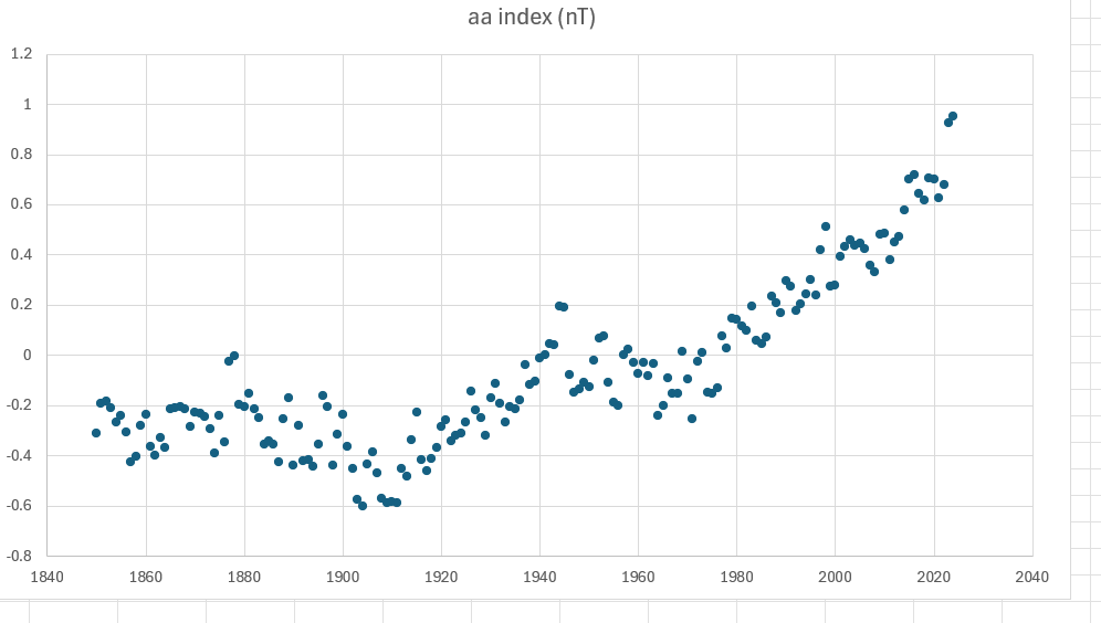
Andy’s spreadsheet has SST data, not aa.
Hi Willis,
I sent your comment (and mine) to Frank to see if he had anything to add, this is what he sent me:
This is a very tricky area to work in. We have intriguing data, but we don’t understand how it all works, only that there are correlations we cannot explain. Certainly the aa index, the AMO, and TSI all seem to affect climate, but in different ways. That is really all we can say at this time.
Andy,
One need be careful when smoothing. I noticed that when asking some of NOAA’s products to do the smoothing that was available for choosing I got some curves that just didn’t fit the raw data properly.
It was most noticable with Tavg, probably because that has two unique distributions that create it. Seasonality also comes into play when looking at monthly data.
It is what got me interested in time series analysis.
“First, it’s not clear where he’s getting his data.”
A bit late to this, but I think the paper says it gets the post 2010 data from the British Geological Survey – but that’s very tedious as you have to get each year separately, and then it only gives you a web table.
However, after much searching I found this page from the ISGI
https://isgi.unistra.fr/data_download.php
Which allows you to download 3 hourly data going back to 1868. You can only download 100 years at a time and you need to provide an email address each time.
Here’s my graph of annual averages along with an 11 year running average.
Your annual average hides uncertainty and the smoothed average hides even more uncertainty. You have not provided any error bars showing the uncertainty derived from the original individual measurements carried forward.
You should begin going through W. M. Briggs classes, they are illuminating.
The Second Biggest Error In Time Series, Class 81
The first quote applies to your assumption that annual averages are real data. They are not. Consequently, you ignore some uncertainty. When you smooth, what you get is not real data, uncertainty is ignored.
“Your annual average hides uncertainty and the smoothed average hides even more uncertainty.”
Do you ever have anything relevant to say? This whole article is about using aa as a forcing to sea temperatures. I mearly pointed someone to where the data can be found. No uncertainty is given. and the 11 year average is the smoothing the paper uses.
“You should begin going through W. M. Briggs classes…”
I see why you keep spouting so much nonsense.
“The first quote applies to your assumption that annual averages are real data.”
It’s not my assumption that this is real data. I have no idea if this particular index is more useful than any other indicator of solar activity. I am mearly showing where you can get the data and what it looks like. I could show you the daily averages or even the 3 hour values if you like, but it’s very messy.
“Consequently, you ignore some uncertainty.”
I am not showing any uncerainty. There are no uncertainty values given in this data source. Showing annual averages makes no difference to that, except the averages will have less uncertainty than the 3 hourly values.
If you think the uncertainty if the data invalidates yhe conclusion of the paper. take it up with the author or Andy May. My own suspicion is the paper is wrong for far bigger reasons than the uncertainty of the aa data. My only interest in downloading the data is to test this for myself.
Exactly! That is my point and it is relevant to what is being discussed.
You posted it as evidence, meaning you accept conclusions made from it.
I don’t accept it as scientific evidence because of the methods and due to the lack of uncertainty. You should consider the value of the evidence before you post.
“You posted it as evidence,”
As evidence that I had downloaded the data. You really demonstrate your obsesion with me – when a simple help in response to request for data leads to these forever disussions about uncertainty.
“I could show you the daily averages or even the 3 hour values if you like, but it’s very messy.”
Here is the 3-hourly index for 2024.
The scale is dominated by spikes caused by solar storms. The two largest spikes were both accompanied by aurora in southern England. This illustrates a problem with the aa index – it’s based on just two positions on the globe. Also it’s evident that the scale has low resolution.
But none of this matters too much when the purpose of the index here is to provide a proxy for solar activity. All that really matters here is to what extent global temperatures change as the average aa changes.
You think that maybe the sun affects the temperature more than 4/10,000ths of the atmosphere that is CO2? Dah! You think that 4/10,000ths CO2 is dangerously high, when the average since life crawled up onto land has been about 37/10,000ths, and as high as 70/10,000? What do you think happens when the atmospheric CO2 drops to 1/10,000? The biosphere begins to die.