By Christopher Monckton of Brenchly
Joe Born (March 12) raises some questions about our paper Why models run hot: results from an irreducibly simple climate model, published in January in the Science Bulletin of the Chinese Academy of Sciences.
To get a copy of our paper, go to scibull.com and click on “Most Read Articles”. By an order of magnitude, our paper is the all-time no. 1 in the journal’s 60-year archive for downloads either of the abstract or of the full text.

Mr Born says that he is not sure he should take on trust our assertion that the Planck or instantaneous climate-sensitivity parameter is about 0.31 Kelvin per Watt per square meter; that we “obscure” the influences on the fraction of equilibrium temperature response attained in a given year; that we have used that fraction “improperly”; that we have incorrectly assumed a steep initial increase in temperature response; that we have relied on a model generated by a step-function representing the effects of a sudden pulse in CO2 concentration rather than one in which concentration increases by little and little; that it is “not clear” how we have determined that the 0.6 K committed but unrealized global warming predicted by the IPCC was not likely to occur; that our model should have taken more explicit account of the fact that different feedbacks operate over different timescales; that we were wrong to state that in an electronic circuit the output voltage transits from the positive to the negative rail at loop gains >1; and that our discussion of electronic circuitry was “unnecessary”.
Phew! I shall answer each of these points briefly.
First, however, Mr Born’s essay is predicated on a fundamental assumption that is flat wrong. He says that increasing CO2 concentration raises the optical density of the atmosphere, in turn raising the effective altitude [so far so good],
“and, lapse rate being what it is, reduces the effective temperature from which the Earth radiates into space, so less heat escapes, and the Earth warms”.
No. The characteristic-emission layer – the “altitude” from which the Earth appears to radiate spaceward, and at which, uniquely in the climate system, the fundamental equation of radiative transfer applies – is the locus of all points at or above the Earth’s surface at which incoming and outgoing radiation are equal. In general, the mean altitude of the locus of these balance-points rises as a greenhouse gas is added to the atmosphere. Thus far, Mr Born is correct.
His fundamental error lies in his assertion that the increase in the Earth’s characteristic-emission altitude reduces the effective temperature at that altitude, “so less heat escapes, and the Earth warms”.
The truth, which follows from the definition of the characteristic-emission layer and from the fundamental equation of radiative transfer that applies uniquely at that layer, is that the Earth’s effective radiating temperature is unaffected by a mere change in the mean altitude of that layer. It is not, as Mr Born says it is, “reduced” as the altitude increases.
The radiative-transfer identity, first derived empirically by the Slovene mathematician Stefan and demonstrated theoretically five years later by his Austrian pupil Ludwig Boltzmann, equates the flux density at the characteristic-emission layer with the product of three parameters: the emissivity of that layer; the Stefan-Boltzmann constant; and the fourth power of temperature.
Now, the flux density is constant, provided that total solar irradiance is constant (which, averaged over the 11-year cycle, it broadly is), and provided that the Earth’s albedo does not change much (it doesn’t). Emissivity is as near constant at unity as makes no difference; and the Stefan-Boltzmann constant is – er – constant. It necessarily follows that the temperature of the emission layer is constant unless any of the other three terms in the equation changes – and none of them changes much, if at all, merely in response to an increase in the mean altitude of the characteristic-emission layer.
Precisely because the effective radiating temperature at the characteristic-emission layer is near-constant under an increase in the mean altitude of the characteristic-emission layer, and precisely because the lapse rate of atmospheric temperature with altitude is very nearly constant under that increase, it is the surface temperature, not the effective radiating temperature at the characteristic-emission altitude, that rises in response to that increase in altitude.
Many of the subsequent errors in Mr Born’s understanding appear to flow from this one.
So to the individual points he makes.
First, the value of the Planck parameter. We stated in our paper that we had accepted the IPCC’s stated value. We might also have explained that we did not take it on trust. Indeed, the first of many fundamental errors in the climate modelers’ methodology that I identified, back in 2006, was the mismatch between the official value 0.31 K W–1 m2 and the Earth’s surface value 0.18 K W–1 m2 that was implicit in Kevin Trenberth’s 1997 paper on the Earth’s radiation budget.
As our paper explains, to a first approximation the Planck parameter is simply the first differential of the fundamental equation of radiative transfer – i.e., 0.27 K W–1 m2. However, allowance for the Hölder inequality obliges us to integrate the differentials latitude by latitude, based on variations in both radiation and temperature. That brings the value up by about one-sixth, to 0.31 K W–1 m2.
To verify that the modelers had done this calculation correctly, I asked John Christy for 30 years’-worth of satellite mid-troposphere temperature anomaly data in latitudinal steps of 2.5 degrees and spent a weekend doing the zenith angles, frustal geometry and integration myself. My value for the Planck parameter agreed with that of the IPCC to three decimal places. And, precisely because all of the parameters in the fundamental equation of radiative transfer are as near constant as makes no difference, the Planck parameter is not going to change all that much in our lifetime.
Next, Mr Born says we “obscure” the influences on the fraction equilibrium temperature response attained a given number of years after a radiative perturbation. Far from it. We begin by making an elementary point somehow not stated by Mr Born: that if there be any feedbacks (whether net-positive or net-negative) operating on the climate object, then the instantaneous and equilibrium temperature responses to a given radiative perturbation will not be identical, and there will be some pathway, over time to equilibrium, by which the temperature response will increase (with net-positive feedbacks) or decrease (with net-negative feedbacks) compared with the instantaneous response.
We continue by explaining the IPCC’s values – in its 2007 and 2013 reports – for the principal temperature feedbacks. We further explain that the response to feedbacks over time is not linear, but (assuming the IPCC’s strongly net-positive feedbacks) follows a curve in which, typically, half the approach to equilibrium occurs in the first 100 years, and the remainder occurs over the next 3000 years (see e.g. Solomon et al., 2009). We also provide a simple table of values over time that are unlikely to introduce too much error. The table was derived from a graph in Gerard Roe’s magisterial paper of 2009 on feedbacks and the climate. Far from obscuring anything, we had made everything explicit.

Mr Born goes on to say we had used the fraction of equilibrium temperature response “improperly”. However, it is trivial that in all runs of our model that concerned equilibrium sensitivity (and most of them did) that fraction is simply unity. In those runs that concerned instantaneous sensitivity (some did), that fraction is simply the ratio of the Planck to the equilibrium sensitivity parameter. In those runs that concerned transient sensitivity, we were dealing with sub-centennial timescales, so that up to half of the equilibrium response should have been evident. All of this is uncontroversial, mainstream climate science. Admittedly, it is very badly explained in the IPCC’s documents: but not the least value of our paper has been in explaining simple concepts such as this one.
Next Mr Born says we have incorrectly assumed a steep initial increase in temperature response (one can see this steep initial response quite clearly in Roe’s graph). Mr Born may or may not be right that there should not be a steep initial increase; but, like it or not, that is the assumption the IPCC and others make. We provided worked examples in the paper to show this. In short, Mr Born’s quarrel on this point is not with us but with the IPCC.
Furthermore, once we had calibrated the model using the IPCC’s assumptions and had obtained much the same sensitivities as it had published, we then adopted assumptions that seemed to us to be less inappropriate, and ran the model to reach our own estimates of climate sensitivity: around 1 K per Co2 doubling.
One of those assumptions, attested to by a growing body of papers in the literature, some dozen of which we cited, is that temperature feedbacks are probably net-negative. Here, for instance, is a graph from Lindzen & Choi (2009), showing the predictions of 11 models compared with measurements from the ERBE and CERES satellites:

Given the probability that temperature feedbacks are net-negative, we ourselves had not assumed a strong initial temperature increase: for that assumption, made by the IPCC, depends crucially on strongly net-positive feedbacks, some of which – such as water vapor – are supposed to be quick-acting. However, the ISCCP data appear to suggest no increase in column water vapor in recent decades, and even something of a decrease at the crucial mid-troposphere altitude:

Mr Born complains that in determining the fraction of equilibrium temperature response at any given year we relied on a model generated by a step-function representing the effects of a sudden pulse in CO2 concentration rather than one in which concentration increases by little and little. So we did: however, as the paper explains, we tested the model to ensure that the results it generated over, say, 100 years were much the same as those of the IPCC. It generated broadly similar results.
As it happens, I had first come across the problem of stimuli occurring not instantaneously but over a term of years when studying the epidemiology of HIV transmission. My then model, adopted by some hospitals in the national health service, overcame the problem by the use of matrix addition, but sensitivity tests showed that assuming a single stimulus all at once produced very little difference compared with the time-smeared stimulus, merely displacing the response by a few years. Similar considerations apply to the climate.
Besides, our model is just that – a model. If Mr Born does not like our values for the fraction of equilibrium temperature response attained after a given period, he is of course free to choose his own values by whatever more complex method he may prefer. But, unless he chooses values that depart a long way from mainstream climate science, the final sensitivities he determines with our simple model will not be vastly different from our own estimates.
Next, Mr Born says it is “not clear” how we have determined that the 0.6 K committed but unrealized global warming predicted by the IPCC was not likely to occur. On the contrary, it is explicitly stated. We assumed ad argumentum that all warming since 1850 was anthropogenic, ran our model and found that the variance between its predicted warming to 2014 and the observed outturn was nil, implying – as explicitly stated in the paper, that there is no committed but unrealized global warming in the pipeline. See table 4 of our paper.
Interestingly, the official answer of the “hokey team” to our point is that we should have assumed that more than all the warming since 1850 was manmade. On that point, we disagree. For They cannot at once argue that the hefty increase in solar activity between the Maunder Minimum 0f 1645-1715 and the near-Grand Maximum of 1925-1995 had no influence on global temperature, but that the decline in solar activity since its peak in 1960 is so great that it would have caused significant cooling in the absence of anthropogenic forcings over the period.

Mr Born also complains that our model should have taken more explicit account of the fact that different feedbacks operate over different timescales. Well, our transience fraction may be tuned at will to take account of that fact. And we even presented a table of values of that fraction over time to take account of a mainstream, conventional distribution of temperature feedbacks and their influences over time. If Mr Born disagrees with Dr Roe’s curve, he is of course entirely free to substitute his own. We presented not tablets of stone but a model.
Next, Mr Born devotes much ink but not much light to his assertion that we were wrong to state that in an electronic circuit the output voltage transits from the positive to the negative rail at loop gains >1. We consulted the reviewed literature; a process engineer with three doctorates, who also consulted the literature; a doctor of climatology specializing in feedback analysis as applied to the Earth’s climate; and a Professor ditto (the last two being among the top six worldwide in this highly specialist field). I also discussed the question of the response-versus-loop-gain curve with a group of IPCC lead authors at a talk I gave at the University of Tasmania three years ago.
Not one of these eminent advisers agrees with Mr Born. That, on its own, does not mean he is wrong: but it does mean that the point we raise is at least respectable.
The Bode feedback-amplification equation is entirely clear: at loop gains >1 the equation mandates that the temperature response becomes negative. In an electronic circuit one can of course – as Mr Born does at rather tedious length – find ways of making the circuit oscillate even in the absence of loop gains >1, and one can find ways of making it not oscillate even at loop gains >1.
However, the equation actually used in the climate models (including ours) is, like it or not, the Bode system-gain equation. Mr Born carefully plots only that part of the graph of the equation below a loop gain of 1:

However, our paper plots the graph both sides of a loop gain of unity. A loop gain of 1 is equivalent to the feedback sum of 3.2 Watts per square meter per Kelvin in Mr Born’s graph, for in the climate the loop gain is the product of the feedback sum and the Planck parameter, and the Planck parameter is the reciprocal of 3.2.

On reading Mr Born’s piece one would think the point we had raised was both trivial and inappropriate. However, the specialists whom we consulted, and the equation itself, suggest that our point is both non-trivial and substantial.
Indeed, the Professor, until I debated the issue with him before a learned society somewhere in Europe a couple of years back, was a true-believer in the profitably catastrophist viewpoint. When I displayed the full plot of the Bode equation he went white.
He wrote to me afterwards, sending me a paper in which he had himself urged caution in the use of Bode in climate modeling. A few weeks ago he got in touch again to say he has thought about the matter ever since and has now concluded – damn you, Monckton – that I am right, and that in consequence climate sensitivity cannot be more than 1 K and may be less.
He has submitted a paper for peer review. If that paper is published, and if it proves correct, the science will indeed be settled – but in a direction entirely uncongenial to the profiteers of doom.
One of the IPCC lead authors in Tasmania interrupted my talk when I showed the full Bode graph and said: “Have you published this?” No, I replied. “But you must,” he said. “This changes everything!” Yes, I said, I rather think it does.
If the Bode equation is inappropriate for loop gains >1, then it may also be inappropriate for loop gains <1. It may – at least in its unmodified form – be the wrong equation altogether. And without it one cannot get away with claiming the absurdly high and unphysical sensitivities the IPCC profits by asking us to believe in.
At minimum, tough asymptotic bounds to constrain the behavior of the equation at the singularity should be imposed. That, at any rate, is what the very small variability of global temperature over the past 810,000 years would suggest: and, on that point, Mr Born surely agrees with us.

The hokey team have responded to this point by saying that the paleoclimate record (showing temperature varying by only 3.5 K either side of the long-run mean over the past 810,000 years) demonstrates high net-positive feedback in response to very small forcings over the period.
Accordingly, I consulted an eminent geologist who said the positive and negative forcings over so long a timescale were very substantial. So I consulted another geologist. He said the same.
Mr Born’s final point is that our discussion of electronic circuitry was “unnecessary”. Not so. The models use an equation taken from electronic circuitry, where it represents a real event, the phase-transition of the voltage from the positive to the negative rail at a loop gain of unity, and misapply it to the climate, which is an object in a class to which that equation does not apply, especially at the very high loop gains implicit in the IPCC’s estimates of climate sensitivity.
There are two principal reasons why the Bode equation – unless it is modified in some fashion analogous to Mr Born’s modification of a circuit to prevent its output from behaving as it would otherwise do – does not apply to the climate.
First, as temperature feedbacks and hence loop gain increase, there comes no moment at which the effect of the feedbacks is to reverse the output and push temperatures down, though that is what the Bode equation in the form in which it is applied to the climate models mandates.
Secondly, in an electronic circuit the output [voltage] is a bare output: it does not act to equilibrate the circuit following the perturbation amplified by the feedback. In the climate, however, an increase in surface temperature is precisely the mechanism by which the object self-equilibrates, and the Bode equation simply does not model this situation.
For these reasons, we considered it important to raise an early red flag about the applicability of the Bode equation. We are not the first to have done so, but as far as we know our brief treatment of the problem is more explicit than anything that has been published before in the reviewed literature.
I have a further paper on the Bode question in the works that has passed review by an eminent expert in the field (I don’t know who, but the journal is in awe of him). The paper will be published in the next few months.

At no point did that reviewer (or any reviewer) question the validity of the point we raised. On the contrary, he said that the paper was a good definition of a real problem. The paper describes the problem in some detail and raises questions designed to lead to a solution.
Readers who have struggled through to this point may now like to read our paper in Science Bulletin for themselves. There is, perhaps, not a lot wrong with it after all.
http://jennifermarohasy.com/2013/12/agw-falsified-noaa-long-wave-radiation-data-incompatible-with-the-theory-of-anthropogenic-global-warming-2/
AGW enthusiast are in denial of the data once again.
For once it would be nice to see them reconcile their theory with the data.
ANTHROPOGENIC Global Warming (AGW) theory claims the earth is warming because rising CO2 is like a blanket, reducing Earth’s energy loss to space. However, data from the US National Oceanic and Atmospheric Administration (NOAA) shows that at least for the last 30 years, Earth’s energy loss to space has been rising.
From the article.
The blanket analogy troubles me. Would not increasing CO2 in the upper atmosphere also act as a reflective shield? If shortwave radiation strikes CO2 in the upper atmosphere it seems as likely to radiate long wave radiation back into space as it would to radiate towards earth? Would this not cause less Albedo effect at the surface?
Monckton of Brenchley
Your very first equation presents &lambda0 as the constant of δT vs δF, this is effectively a classic first order linear ODE, of the simplest kind. It describes a linear feedback and &lambda0 “sensitivity parameter” is that feedback.
The ODE would normally have a negative sign which defines the feedback as negative but this is simply a case of the convention of which direction is considered positive heat flux in climate. In engineering the greater heat flux opposes the increased temperature so it would be negative.
This is mainly a problem of adopting the rather unscientific language of IPCC: talking of “net positive ” feedbacks when they really mean “less negative” feedback, but it is important if you are writing scientific papers to clear about the terms and what they represent physically.
This term represents how “sensitive” climate is, because it is a feedback.
&lambda0 “sensitivity parameter”: the Plack feedback is indeed a feedback. It is the main feedback. which stabilises the climate system and that is why all other feedbacks are considered relative to the Planck feedback.
All your other feedbacks are stated as a proportion of Planck sensitivity: &lambda0 ft
This purely linear approximation to T^4 is fine for deviations of the order of 0.1K, in equilibrium temperature. The guts of the models will be using T^4 for actual spot temperature physics.
However, if they start to discuss 2K deviations or some of the more fanciful figures like 4-6 kelvin of warming then the non linear form will be required. A supposedly linear sensitivity will start to reduce if such a significant warming is produced. This was found to be the case by Paul_K whose article I linked above. Models do not display fixed linear sensitivities at higher dT.
This is where the asymptotic rise to infinity falls apart. Like in the electronic amplifier, the continued rise is irrelevant because it is physically meaningless and will not happen. Any discussion of going over the top *through infinity* to re-emerge the other side and flipping sign is nonsense.
Whatever any particular electronic circuit does when you try to drive it like that is entirely determined by the undocumented, NON-linear behaviour it exhibits when driven beyond its design parameters. Whether it latches up, burns out or oscillates, tells us nothing about climate nor the linear system it follows under normal operation. Your electronics experts should have explained that to you.
The Planck “feedback” is not a feedback. It is not treated as such in the standard equations of climate sensitivity. It is better regarded as a zero-feedback climate-sensitivity parameter, by which a direct forcing is multiplied to obtain the temperature change caused by that forcing in the absence of any feedbacks. The product of the feedback-sum and the Planck parameter is then the loop gain in the system.
When sufficient feedback occurs in an electronic circuit to drive the loop gain above unity, the current goes around the circuit the other way, so that the output voltage that had been positive suddenly becomes negative. I have seen this explicitly mentioned in the specialist literature, and it was confirmed by the eminent process engineer whom I consulted in detail. Also, my paper providing a more detailed consideration of this question has passed peer review at the hands of another even more eminent specialist and will be published next month.
The climate, in various fundamental respects, does not behave like an electronic circuit. See the head posting. The Bode equation, therefore, is the wrong equation and requires to be modified or replaced to remove the absurd exaggerations of climate sensitivity to which its use gives rise.
Thanks for your reply but I think you have a misunderstanding here.
Climate sensitivity, as defined in the simple linear equation is a diagnostic of model ( or climate ) behaviour. Climate models at the detailed physics level of thier calculations at each grid point use T^4 S-B derviced equations. It is in analysing the model output that attempts are made to characterise its behaviour in terms of a simplified constant linear parameter.
Thus climate sensitivity is an emergent property, not one that is programmed in.
You suggested the GISS model does this, can you provide a direct link to the Hansen papers from which you say you got this conclusion?
” It is better regarded as a zero-feedback climate-sensitivity parameter”
That is self contradictory. with zero feedback there would be no “sensitivity”. The slightest δF would cause continual warming and the system would be unstable. It is better to call it what it is : the greatest f/b which ensures the system is stable.
Again you are falling for IPCC linguistic games. Like perfectly normal temperature deviations are called “anomalies” in order to imply from the outset that any change is “abnormal”, the idea of “net positive” feedbacks implies instability, when in fact it is just a misrepresentation of “less negative” feedback, or *slightly* less stable.
This leads to the idea of “tipping points” which is non-sense. Nothing is going to overpower a T^4 neg. f/b. You should challenge this language not adopt it.
Planck IS a feedback and it is the sole reason we are here to have the this discussion.
“When sufficient feedback occurs in an electronic circuit to drive the loop gain above unity, the current goes around the circuit the other way ….”
As I explained in detail above, this kind of talk is meaningless. It depends totally upon how a particular circuit design FAILS to remain linear when run outside it’s design parameters. It tells you nothing about linear systems because it is no longer linear. This is akin to speculating what happens on the other side of the mathematical singularity at a blackhole ( should such a thing exist ).
A nuclear fission explosion is probably the most dramatic illustration of a positive feedback and even that eventually is constrained by negative feedbacks. The explosion is localised. The whole world does not explode and we don’t pop out of the other side with energy flowing in the other direction !
I suggest you limit yourself to pointing out there are limits as to how far linearity can be used as a reasonable approximation. You are going well beyond what you understand here and risk destroying any credibility that you may have accrued by your efforts.
The paper is apparently stirring a few thoughts among simplistic climatologists and is probably a useful explanation of the use of the linear model. Try not to undo that.
What you are calling the Bode equation is not specific to electronics. It can be applied, simplistically to many physical systems. Knowing when it fails to apply, either in electronics or any other application is essential to proper use. It is not more or less applicable to climate because it is used in electronics.
This is another logical error that you have been promulgating for some time.
Best regards.
Mr Goodman is misunderstanding various matters. First, the equation for climate sensitivity is non-linear in that the fundamental equation of radiative transfer is a fourth-power relation, and again non-linear in that the CO2 forcing function is logarithmic; and again non-linear in that most feedbacks are non-linear (see the appendix to our paper for this), and again non-linear in that response times are non-linear, and again non-linear in that the object under discussion behaves as a chaotic object.
Next, climate sensitivity may be an input to or an output from the model, depending upon its design. In our model, climate sensitivity is an output.
Next, it is incorrect to say that in the absence of feedbacks there would be no climate sensitivity, and additionally incorrect to say that without feedbacks the object must be unstable. The mean value of the Planck or zero-feedback sensitivity parameter is about 0.3125 Kelvin per Watt per square meter of direct radiative forcing. Multiply that parameter by the forcing and the climate sensitivity in the absence of temperature feedbacks emerges: thus, where the forcing in response to doubled CO2 concentration is 5.35 times the logarithm of 2, or 0.69 Watts per square meter, the zero-feedback climate sensitivity is about 1.16 K – not exactly an unstable result.
It is where the feedbacks are imagined to be strongly net-positive that the instability arises, as the plot of the singularity in the Bode equation makes clear.
The Bode equation also shows what happens to the output voltage in an amplifier where the closed-loop gain exceeds unity. What was a drive towards positive infinity becomes a drive towards negative infinity in the voltage. Circuits can thus be made to oscillate by driving the loop gain above unity and then relaxing it back below unity again. There is plenty of literature on this. Try search for “from the positive rail to the negative rail”, for instance, or study “feedback-induced oscillation”. Or build a robust circuit and try it out.
However, in the climate a loop gain of more than 1 would not produce a plunge in temperature. In this and in other respects (see my forthcoming paper), the Bode equation does not – whether you or I like it or not – satisfactorily model the climate. We are not the first to have pointed this out in the literature, though we have been more explicit than anyone to date in expressing our concerns.
The Bode equation requires modification or replacement before it can be legitimately applied to the climate object. If peer review of a paper by an eminent professor who specializes in this field is successful, the extent to which Bode does not apply to the climate will become clear to all.
I am well aware that the Bode equation applies not only to electronic circuits but also to a class of dynamical systems. The climate is not, repeat not, in that class.
Monckton of Brenchley March 18, 2015 at 9:47 am
Mr Goodman is misunderstanding various matters. First, the equation for climate sensitivity is non-linear in that the fundamental equation of radiative transfer is a fourth-power relation, and again non-linear in that the CO2 forcing function is logarithmic; and again non-linear in that most feedbacks are non-linear (see the appendix to our paper for this), and again non-linear in that response times are non-linear, and again non-linear in that the object under discussion behaves as a chaotic object.
As you admitted in an earlier conversation that Appendix doesn’t exist, perhaps you can make it available here?
The Bode equation also shows what happens to the output voltage in an amplifier where the closed-loop gain exceeds unity. What was a drive towards positive infinity becomes a drive towards negative infinity in the voltage. Circuits can thus be made to oscillate by driving the loop gain above unity and then relaxing it back below unity again.
No, the loop gain does not change, the nature of the stationary point changes to an unstable focus and follows an oscillatory path to a stable limit cycle. See the Wien bridge oscillator for an example, gain of 0.99 = stable operation, 1.01 = oscillation (sine wave), 1.50 = distorted oscillation.
There’s actually nothing wrong with using the electronic analogy since the linear description of such circuits is a simplified model as is that of climate. The same degree of understanding of the limits of the linear approximation are required but within that limit there is no reason to suggest it is not proper because it only applies to electronics. This is not the case. Many other systems are modelled and analysed as linear simplifications.
What you need to model is an operational amplifier ( op-amp ) with strong negative feedback. The discussion of climate sensitivity is then adding a little more neg. f/b or a little +/ve f/b. This can be done in couple of minutes with a 741 on a bit “breadboard” or on paper. It’s first year electronics.
The deviations of the output voltage caused by a predefined disturbance at the input can be studied. In the case where some +ve f/b is added the output voltage will vary more than the untampered “Planck” amplifier: it more “sensitive”. Conversely, with more negative f/b the amp output will change less: it is less “sensitive”.
One could then add some RC networks into the circuit and make an analogue computer model for the climate system, with single slab, or multiple slab ocean heat capacities. Three such amps could be set up with different sensitivities, one for the tropics an one each for NH SH extra-tropical zones. Suitable linkage between the outputs to reflect inter-zone heat transfer.
Add a resistor chain and an push button to simulate volcanoes. You can take the analogy as far as you like.
Just realise what the Planck term is before you start. 😉
What a fantastic thread!
Slightly off topic, but I cannot help myself:
Where are the trolls?
In thread after thread we are inundated with trolls explaining to us how stupid we are, most quote the much worn out 97% consensus meme or similar appeal to authority, some claim to be “teachers” of climate science, but wilt when asked to discuss the actual science. So where are they? Here the science is being debated at its most raw level, with heavy weights, light weights, and interested observers arguing, supporting, refining, discussing the science.
But from the trolls, not a peep. You’d think with their vaunted superiority they’d be thick as thieves in this thread, explaining the facts to us. Seems when actual science is on the table… they scurry away in fear of making fools of themselves by entering the fray.
Mr Hoffer is right. This thread has been a real pleasure because on all sides there has been a willingness to discuss the science. Indeed, the object of our paper was to make climate – sensitivity math widely accessible without excessive simplification.
Isn’t gain in electronics the same as infinite series in mathematics?
for example:
1/2+1/4+1/8+1/16…..
this infinite series has a finite answer.
while a series like:
1/1+1/2+1/3+1/4+1/5 …
does not.
and a series like
1+3+9+27….
most definitely does not!
So for feedback to be stable, it seems it must at the limit be an infinite series with a result that is less than infinity.
correction, isn’t feedback gain the same …
Exactly.
The particular series that’s analogous here is a power series like your first and last, which take the form 1 + r + r^2 + r^3 + . . . .
Lord Monckton’s theory is analogous to saying that the sum is negative if r > 0; your last series 1 + 3 + 9 + . . . sums to a negative value according to Lord Monckton’s way of looking at things.
Why? Well, if S = 1 + r + r^2 + r^3 + . , then rS = r + r^2 + . . ., so S – rS = (1 – r) S = 1, so S = 1 / (1 – r), which is negative for r > 1.
Math is tricky, especially when you work with infinities.
My final say on this thread. We have directly measured the potential affects of TSI on global warming. This is not a model. This is a measurement from satellites. The change in watts per meter squared of incoming solar radiation from a busy Sun to a quiet Sun is known. Physics then tells us the possible change in temperature in Celsius and Fahrenheit the change in watts/m2 can possibly have on our temperatures here on Earth.
The above various proponents of Solar-driven reasons for the recent warming know this so they instead depend on a variety of unobserved amplification mechanisms. It smacks of the CO2 water vapor amplification mechanism proffered from the other camp. Which is also unobserved.
http://phys.org/pdf129483836.pdf
So to both I say, you are ignoring an incredibly variable and complex planet. One that can strike out incoming solar irradiance change to its knees and home-run the change up pitch of CO2 over the fence. Earth wins the game. Not CO2 and not Solar variation.
Pamela Gray wrote, “My final say on this thread. We have directly measured the potential affects of TSI on global warming. This is not a model. This is a measurement from satellites. The change in watts per meter squared of incoming solar radiation from a busy Sun to a quiet Sun is known.”
Your statement is not actually correct. TSI has been measured from what was deemed an active sun and what was deemed a quite sun. TSI HAS NOT been measured when the sun was in grand minimum with no sun spots most years. Perhaps TSI does drop predictably as the number of sun spots declines. But how much does it drop when sun spots hit zero for a time?
No one knows how low the solar emissions are in a grand minimum. Some solar physicists think that the sun probably is not very variable and put an estimate to the variation that they think is possible and most have used that kind of estimate. But the problem is that stars that are deemed by astronomers to be very similar to ours have shown quite a bit more variation than the solar physicists are deeming possible for our sun.
A grand minimum could have TSI dropping quite a bit more than has ever been measured in modern times.
No one knows how low the solar emissions are in a grand minimum
This cuts both ways. If correct you cannot assume that TSI was much lower during a grand minimum.
And there are other ways of getting at this, e.g. http://climateaudit.org/2007/11/30/svalgaard-solar-theory/
lsvalgaard wrote, “And there are other ways of getting at this, e.g. http://climateaudit.org/2007/11/30/svalgaard-solar-theory/ ”
I studied the information in the link. From a scale of 1 to 10 where 10 is a fairly strong scientific conclusion, I would rate it as a 1 only because there is no lower number. On the other hand, your solar sunspot number reconstruction – I would rate it at a 10.
From the link to Svalgaard Solar Theory “The existence of floors in IMF and FUV over ~1.6 centuries argues for a lack of secular variations of these parameters on that time scale. . The five lines of evidence discussed above suggest that the lack of such secular variation undermines the circumstantial evidence for a hidden source of irradiance variability and that there therefore also might be a floor in TSI, such that TSI during Grand Minima would simply be that observed at current solar minima.”
No it doesn’t! You have one very short sample time period in the “life” of the sun. It is not significant. Especially when solar physics models of the sun are not able to determine yet how variable the sun is or what the changes in TSI will be based on variability.
To form meaningful lines of evidence in the way you tried, the theoretical background needs to be much more settled.
Especially when solar physics models of the sun are not able to determine yet how variable the sun is or what the changes in TSI will be based on variability
On what do you base that? We measure how variable the Sun is on time scales of interest [centuries].
Well, you may have studied the link, but you failed to appreciate the information given. The radiative output [TSI] is observed to have two component: (1) that comes from the core of the Sun and (2) one that due to the magnetic field at the surface. Some spectral lines are very temperature sensitive. Such lines have been carefully monitored for many decades in areas where there were no sunspots and no observable magnetic fields. The results show that there is no solar cycle variation of this ‘basal’ temperature, it is indeed constant, so would not be expected to be any different during a grand minimum. If you disagree, then you have to produce evidence that there would a difference. The magnetic component of TSI has also been carefully monitored for decades and show that it is accounted for by the observed magnetic field and that there is no mystery about this.
lsvalgaard wrote, “On what do you base that? We measure how variable the Sun is on time scales of interest [centuries].”
The time period “of interest” that has been observed still does not include a grand solar minimum similar to the Maunder Minimum. In fact, without having a robust theoretical understanding of solar variability, it is not scientifically robust to simply pick a time period and from that time period, be able to make robust determinations of what may happen in longer time period given the current knowledge of solar physics.
lsvalgaard wrote, “Well, you may have studied the link, but you failed to appreciate the information given. The radiative output [TSI] is observed to have two component: (1) that comes from the core of the Sun and (2) one that due to the magnetic field at the surface. ”
The information suffers from the same problem as above. You really can’t determine how much time you must observe the sun in order to determine if you have a good sample of it’s variability.
lsvalgaard wrote, “The results show that there is no solar cycle variation of this ‘basal’ temperature, it is indeed constant, so would not be expected to be any different during a grand minimum.”
That it would be no different in a grand minimum is an untested hypothesis based on very little.
lsvalgaard wrote, “If you disagree, then you have to produce evidence that there would a difference.”
No, it is your hypothesis. You need to find a better way to test it. Although the next couple solar cycles might help with that if there is a long period with no sun spots.
I am pointing out that your hypothesis is based on insufficient data and lacks a firm theoretical (solar physics) foundation. In my opinion, it is more conjecture than hypothesis.
Well, I think we have a good understanding of how this works. I spelled it out for you, but to no avail. The null hypothesis must be that there are no unknowns lurking about. All the data we have say that the basal temperature [and thus base TSI] does not change, and that the additional irradiance is simply that due to magnetic activity.
That it would be no different in a grand minimum is an untested hypothesis based on very little.
The untested hypothesis is that it would be different. On what do you base that?
lacks a firm theoretical (solar physics) foundation
I explained to you what the firm theoretical foundation is. Here it is again: TSI has two components: one that comes from the energy producing core taking hundreds of thousands of years to make it to the surface and therefore must be constant on time scales of centuries, and one [a very small part: 1/1000 of the base] that is driven by the magnetic field which varies in the well-known sunspot cycle. Taking away the latter at most changes TSI by 1/1000th as we saw it in 2008-2009.
Yet another example I fear of folks who talk Solar, but who have not availed themselves of a basic current education in solar mechanics and physics. And I do mean from a proper textbook, not the internet.
lsvalgaard, “Well, I think we have a good understanding of how this works. I spelled it out for you, but to no avail. The null hypothesis must be that there are no unknowns lurking about. All the data we have say that the basal temperature [and thus base TSI] does not change, and that the additional irradiance is simply that due to magnetic activity.”
Being interested in the topic, I follow astronomical papers on what has been found with respect to changes in TSI and irradiance in similar stars to our own. I also would note that I’ve read a large number of papers and many have stated explicitly that it is unknown if TSI varies enough to explain the temperature changes seen in the Maunder Minimum.
Example paragraph 1, page 29 of a PHd dissertation by William T. Ball:
” In Fig. 1.2, taken from Hall and Lockwood (2004),
the S-index from 3709 observations of 57 Sun-like stars are plotted as the black histogram.
Measurements of the Sun are plotted as the white histogram outline, with the
y-scale reduced by a factor of 3; the grey histogram are a subset of stars with essentially
flat time series, as discussed in Hall and Lockwood (2004). The implication from this plot
is that the Sun may vary more than current observations suggest, as the S-index from the
stars in this plot lie outside the Sun’s observed range approximately a third of the time
(Haigh et al., 2005). Since magnetic activity is related to changes in luminosity, this has
implications for the amount of energy received from the Sun at Earth. Therefore, solar
analogs and their properties need to be accurately determined over long periods of time
to precisely place the Sun among them. The conclusion from solar analog studies is that
the range of possible fluctuations in the Sun may be very much greater than that currently
observed. However, cosmogenic isotopes suggest that the Sun has been unusually active
in recent decades (Solanki et al., 2004; Steinhilber et al., 2008). These results lead to the
question, how significant an effect on terrestrial climate can the Sun have, and over what
time scales?”
http://wwwf.imperial.ac.uk/~wtb08/files/phd_will_ball_2012.pdf
It is a recent dissertation which is why I picked it as the author has recently looked over the available research.
The dissertation also happens to discuss at length the pros and cons of your position – that base TSI varies little and discusses most of your “evidence”.
I could post various papers supporting the same points. There supporting evidence is that the earth does cool more than would be expected during periods like the Maunder Minimum if TSI varies little below the base value. And the fact that other similar stars to ours are more variable also is more circumstantial evidence. The fact that other stars are less variable may simply be due to the the fact that the period over which stars vary could be greater than the few decades of time astronomers had instruments capable of doing this type of study.
To restate my viewpoint. I’m a skeptic about this. I don’t know if TSI varies much below the “base” case that has currently been established. The evidence you present is unconvincing and circumstantial. Especially given there is no direct measurements of TSI or irradiance during a Maunder minimum type period and the fact that there is direct evidence that the temperature of the earth tends to be colder than normal in grand minumum type periods and the direct evidence that other similar stars to ours have been observed to vary more than our own sun – I think the matter is still undecided.
There are VERY few really sun-like stars that are well observed. The general consensus is that the stars in question are later in their evolution than the Sun.
I think the matter is still undecided
Indeed, some people have a hard time giving up cherished views.
However, cosmogenic isotopes suggest that the Sun has been unusually active in recent decades
The cosmogenic proxies are hard to calibrate and are influenced much by climate and are different at different locations, e.g. http://arxiv.org/ftp/arxiv/papers/1004/1004.2675.pdf and http://arxiv.org/ftp/arxiv/papers/1003/1003.4989.pdf
From direct solar observations it is now clear that there was no such Grand Modern Maximum. Even the Steinhilber paper you cite in support of this shows that, e.g. Slide 20 of http://www.leif.org/research/Does%20The%20Sun%20Vary%20Enough.pdf
As Ball points out:
“all variations in solar irradiance are caused by changes in surface magnetic flux emergence”
which is an observed quantity and cannot go below zero implying a floor or basal value.
The Ball paper compares the [heavily tweaked] SATIRE model with observations of TSI and concludes: “The most important result is that the model recreates the change in TSI between the solar cycle minima of 1996 and 2008, in agreement with the change estimated by the PMOD composite”
However it is now clear that the PMOD composite is wrong in asserting such a decrease, there is uncompensated degradation in the PMOD instruments as first pointed out by me here http://www.leif.org/research/PMOD%20TSI-SOHO%20keyhole%20effect-degradation%20over%20time.pdf and continuing to this day. This degradation was eventually admitted to by the experimenters, e.g. Slide 29 of http://www.leif.org/research/The%20long-term%20variation%20of%20solar%20activity.pdf [Schmutz, 2011]. Bottom line: TSI at the recent minimum was not lower than at previous minima, in addition a good proxy for EUV [and thus the magnetic flux] shows that all the way back to the 1830s the flux at every minimum has been constant, see http://www.leif.org/research/Reconstruction-Solar-EUV-Flux.pdf
so it seems that people will go to great length to try to conform with current dogma.
Now, it is possible that solar magnetic activity as observed is larger on average than on most solar-like stars, but that does not mean that the basal value of TSI follows suit. Different Chemical composition and evolutionary history including formation of planetary systems are likely to cause differences in the level of TSI, but since on century [or even millions of years] timescales those parameters don’t change for the Sun we don’t need to worry about them.
BobG March 18, 2015 at 6:46 pm
I also would note that I’ve read a large number of papers and many have stated explicitly that it is unknown if TSI varies enough to explain the temperature changes seen in the Maunder Minimum.
And yet, you use such a relationship as support for your large variation of TSI. In spite of the difficulty of finding solar analogs [same age, composition, planetary systems, etc.] progress has been made. This paper http://arxiv.org/pdf/1207.0176v1.pdf is a good review of the current state of the art. They conclude “This consequence exclude the possibility for the existence of a considerable fraction (e.g., ∼ 1/3) of “Maunder-minimum stars” such that having activities significantly lower than the current solar-minimum level as once suggested by Baliunas and Jastrow (1990).” and “This excludes the once-suggested possibility for the high frequency of Maunder-minimum stars showing appreciably lower activities than the minimum-Sun”. and “our Sun belongs to the group of manifestly low activity level among solar analogs, the fraction of stars below which is essentially insignificant”. Thus, the Sun does not vary a lot more than commonly thought, it already belongs to a class of low-activity stars.
lsvalgaard wrote, “The difference between us is that you think that because something is undecided it is legitimate to assume that it is true.”
What I believe is that if there is not enough evidence, there is not enough evidence. Generally speaking, most new hypothesis and ideas people come up with can be ruled out with logic and science. I look at any new hypothesis or scientific view from the point of view of can I disprove it or rule it out?
lsvalgaard wrote, ” Al Gore, it is rumored, once said “if you don’t know anything, everything is possible”. ”
Well, if you told Al Gore your hypothesis, then I’m sure he would think it is true.
lsvalgaard wrote, “The physical basis of SATIRE-S is that all variations in solar irradiance are caused by changes in surface magnetic flux emergence
which means that given [we see that observationally] that all variations are caused by changes in surface magnetic flux emergence that is a good basis for the model. Your accusation of ‘out of context’ is thus misplaced. I’ll assume that was just based on ignorance without further intentions.”
You obviously didn’t read his entire thesis. The point of view of the view of the author is that SATIRE-S was a model which quite possibly is wrong.
lsvalgaard wrote, “”You should read the paper I directed you to. http://arxiv.org/pdf/1207.0176v1.pdf that concludes that “our Sun belongs to the group of manifestly low activity level among solar analogs, the fraction of stars below which is essentially insignificant”. ”
I had read it. And this is one of my points. The sun AT THIS TIME seems to be a star that has low activity among solar analogs. Is this observational bias (due to when the observations have been made)? That is a common possibility listed in similar papers. My point is that the fact that there are many stars that are more active and about 10% or so (from the same paper you cited) seem to have lower activity fits right in with what would be expected if periods of low activity where the solar cycle is low happens periodically. Which means that we may not have seen our sun in a period of lower activity.
I do think this question though will be answered in the next 20 years to my satisfaction with more stars that are observationally similar to ours being observed for longer periods. Also, if the next two solar cycles are small and with low numbers of sun spots, we will see evidence if TSI trends below the “base” or not.
The point of view of the view of the author is that SATIRE-S was a model which quite possibly is wrong.
He certainly hides that well when he says that the model “provides an unbiased comparison of the composites of direct radiometric observations of total solar irradiance (TSI), which began in 1978. The excellent agreement with, in particular, the PMOD composite supports the simple model assumptions.”
The point of the stellar connection paper was that “our Sun belongs to the group of manifestly low activity level among solar analogs, the fraction of stars below which is essentially insignificant”. So the chance that the Sun would jump down to become part of that ‘insignificant’ fraction would be insignificant. The Sun is essentially as low as it can go at sunspot minimum. This is also the finding [from helioseismology] of the Goode & Dziembowski paper [confirmed observationally by Berger et al. 2007] concluding that the Sun cannot have been any dimmer than it is now at activity minimum, and the Schrijver et al. paper (2011) that “therefore, the best estimate of magnetic activity, and presumably TSI, for the least‐active Maunder Minimum phases appears to be provided by direct measurement in 2008–2009.”
Now, I realize that probably no amount of argument [or data] can move you off your position, but I think I have demonstrated that a score of ‘1’ that you opened with is a bit unjustified. The observations have moved me to my present view, much to my chagrin.
lsvalgaard wrote, “There are VERY few really sun-like stars that are well observed. The general consensus is that the stars in question are later in their evolution than the Sun.
I think the matter is still undecided
Indeed, some people have a hard time giving up cherished views.”
When I read that last sentence of yours, I had to laugh because I was thinking the same thing about you.
I disagree with you about the general consensus. I think the general consensus is that this point is undecided. Also, the evidence I’ve read indicates at least a couple of the very few stars studied that are more variable are not farther in their evolution than the sun. Should this be further substantiated, it only takes one counterexample to destroy the most finely wrought hypothesis. Of course, a more robust understanding of the physics involved which might be determined in the future would be a good way to settle it also.
Lastly, you wrote – perhaps somewhat wickedly to see if it would be noticed, “As Ball points out:
“all variations in solar irradiance are caused by changes in surface magnetic flux emergence””
This statement is out of the correct context – as I’m sure you knew. He is talking about the model. Putting it in the correct context, he wrote, “The physical basis of SATIRE-S is that all variations in solar irradiance are
caused by changes in surface magnetic flux emergence.”
My views have been arrived at after a long struggle, and grudgingly at that. The difference between us is that you think that because something is undecided it is legitimate to assume that it is true. Al Gore, it is rumored, once said “if you don’t know anything, everything is possible”. With knowledge [which I in all modesty profess to have on this subject] the possibilities shrink dramatically and one may be forced to accept something, much against one’s will.
The physical basis of SATIRE-S is that all variations in solar irradiance are caused by changes in surface magnetic flux emergence
which means that given [we see that observationally] that all variations are caused by changes in surface magnetic flux emergence that is a good basis for the model. Your accusation of ‘out of context’ is thus misplaced. I’ll assume that was just based on ignorance without further intentions.
Also, the evidence I’ve read indicates at least a couple of the very few stars studied that are more variable are not farther in their evolution than the sun
You should read the paper I directed you to. http://arxiv.org/pdf/1207.0176v1.pdf that concludes that “our Sun belongs to the group of manifestly low activity level among solar analogs, the fraction of stars below which is essentially insignificant”. Thus, the Sun does not vary a lot more than commonly thought, it already belongs to a class of low-activity stars. I.e. the sun does not vary much, unlike some stars that do. This is precisely the point: It is not the case that the existence of stars that vary more means that the sun also does, indeed, it does not, contrary to what was thought earlier by some people.
http://www.google.com/url?sa=t&rct=j&q=&esrc=s&source=web&cd=1&ved=0CB4QFjAA&url=http%3A%2F%2Fiopscience.iop.org%2F2041-8205%2F781%2F1%2FL7%2Fpdf%2F2041-8205_781_1_L7.pdf&ei=LFkLVbS8NZa1sQTmh4HYBA&usg=AFQjCNEW4wlbTpJ6LDCUhjHi084GjOnSvw
Bob , this shows the latest work by Professor Lockwood which lends much support to your position and mine on variability of the sun. This is very recent research and less then a year old.
Professor Lockwood estimates solar wind speeds less then 300 km/sec during the Maunder Minimum.
It may be less than a year old, but they still didn’t get it quite right, see
http://www.leif.org/research/Confronting-Models-with-Reconstructions-and-Data.pdf
On the positive side, Lockwood et al. are finally catching up with our 2003 paper
http://www.leif.org/research/Determination%20IMF,%20SW,%20EUV,%201890-2003.pdf
and for that glorious achievement they should be congratulated.
Bob G. Professor Lockwood study validates many of the points you have brought up, and as this prolonged solar minimum continues we will find out where matters stand.
It is difficult to sort out the issues in a discussion of a particular (mathematical) feedback equation which is clear, and the performance of a particular electronic circuit which only feels “obliged” to obey that equation within a certain realm. This is why we do EXPERIMENTS (easy in electronics!); to find the truth.
Back in November of 2013 (motivated by some feedback issue – probably here) I set out to write up a “few pages” and post them on my Electronotes site. It did get out of hand, 24 pages, but NOT lost in technical details (in my opinion). I think it is quite readable. It is here:
http://electronotes.netfirms.com/EN219.pdf
Calling attention to Fig. 12, a positive feedback of +2, I have a test circuit (similar to others there). This one has what looks like a correct analysis, suggesting a resulting gain of -1, CROSSED OUT with orange lines! The analysis was BOGUS (see green measured numbers) because the first op-amp failed as a “virtual ground” because the NEGATIVE feedback (on which the op-amp summer is based) failed.
Just a warning note from the test bench – nothing more.
Thank you for the link.
I haven’t read it yet, but a quick scan confirms–as if confirmation had been needed–that I wasn’t breaking new ground by discussion a loop gain g > 1 circuit.
Incidentally, although I responded to your previous question by saying that because frequency analysis wasn’t germane I hadn’t looked at it much, that question made me think about what it was his consultants told Lord Monckton that made him take away the circuit misapprehension from which none of us has been able to budge him. As often happens, I got distracted before I really completed the math, but I think I would have found found that the result isn’t too surprising.
For non-zero frequencies, I believe, the overall gain remains finite through g = 1 but undergoes a phase reversal there. And, of course, the homogeneous solution blows up beyond g = 1. That’s probably what Lord Monckton heard, and he conflated the two concepts: there’s a phase reversal at g = 1, and the non-driven response component causes the amplifier to get pinned to the supply rail.
What I think I’d also find is that theoretically the sign of the homogeneous solution–i.e., the rail the amplifier gets pinned to–depends on the phase at which the sinusoidal stimulus starts, with one particular phase resulting, only theoretically, of course, in no homogeneous component at all. (In practice, of course, the stimulus is never precisely what we think, and the circuit isn’t either, so which rail it gets pinned to in practice is probably unpredictable.)
Joe – thanks for all you write.
I did see your response comments on your original circuit. You were (too?) quick to note that I got the zero position right. This was a surprise to me because I had just concluded that I got it wrong! I think it depends on A, so that’s why we both see different answers. Anyway, your original circuit has that capacitor so it does have a pole and a first-order low-pass filter in the feedback loop. [The DC “gain” is the resistive voltage divider and the “RC time constant” is the parallel combination of the two R’s, times C. Thevenin equivalent. Thus the magnitude of the feedback rolls off below the attenuation of the voltage-divider, and phase approaches 90 degrees so that the feedback is no longer purely positive. I need to work this out and verify experimentally. ] As you noted, we are probably not particularly interested in frequency response. Step response is more revealing here. Yours seems a good way to represent a delay.
None of my ANALOG circuits has a capacitor so no frequency dependence. Just gain changes. The discrete-time networks DO have a frequency dependence (a pole) because they have a delay, and the delay is a “phase shift” according to frequency.
Still more to learn. Email me (Google my name or Electronotes) if you want to know if I am posting anything. I guess the main lesson is to be careful.
Bernie
Someone still needs to address my fundamental point that the effective emission height and surface temperature need not change at all in the presence of radiative gases radiating direct to space from within the atmosphere because less kinetic energy must then be returned to the surface in convective descent than was taken up from the surface in convective ascent.
That reduced kinetic energy returning to the surface in adiabatic descent offsets the potential surface warming effect of GHGs so that no change in surface temperature or effective emission height is required
Anyone?
The line in the sand you draw is an imaginary one, one in which the theoretical EEH is where its temperature matches that of Earth’s surface. Your conjecture is based on something that cannot be measured.
Pamela,
I don’t follow that at all.
The surface at 288K is obviously higher than the temperature that radiates to space (255K) and the lapse rate slope separates the two and then continues on to the cold of space.
That ‘extra’ surface 33K is constantly cycled up and down adiabatically and retained within the mass of the atmosphere in the form of potential energy in the less dense gases above the surface layer.
Stephen,
There is no ‘Earth temperature’ radiating to space at all. There is only an average final/total radiative flux from the system as a whole of 239 W/m2. This flux is what it is, not because of the physical temperature of some 2D layer somewhere inside the 3D volume of the radiating system, but because the system in question happens to absorb an average flux coming in from the Sun. Heat out simply balances heat in. On average.
A 239 W/m2 emissive flux density is simply mathematically related to a blackbody surface temperature (through the Stefan-Boltzmann equation) at 255K. IF the Earth radiated its entire emission flux to space from ONE specific 2D blackbody surface, then this surface would have to be at 255K.
But the Earth doesn’t radiate its entire emission flux to space from one such BB surface. It radiates from its entire 3D volume, from solid/liquid surface to the ToA, and from all gassy layers in between. Only the final, accumulated flux, the one moving out through the ToA to space, amounts to 239 W/m2. Everywhere below, it’s less, starting out as ~53 W/m2 escaping the actual surface, but also, up through the tropospheric column, turning the energy brought from the surface into the atmosphere by way of conduction and evaporation (24+88= 112 W/m2) into radiative heat to space and finally the solar heat absorbed by the atmosphere on its way down (75 W/m2). Everything is safely radiated back out to space after having done its heating job. To balance the incoming. All that enters also exits. There is nothing of the incoming from the Sun brought back to the surface to do more heating, to somehow raise temperatures ‘further’, neither by “back radiation” nor by “adiabatic descent”.
Kristian said:
“Heat out simply balances heat in. On average.”
That is correct but additonally one has an energy exchange between the mass of the surface and the mass of the atmosphere. The energy content of that exchange (KE low down and PE high up) remains in place for as long as the mass of the atmosphere is suspended off the surface.
To find actual surface temperature as opposed to the S-B radiative calculation one has to add the kinetic energy being exchanged between surface and atmosphere at the surface to the kinetic energy at the surface derived from the S-B equation.
For Earth that results in a surface temperature elevated above S-B by 33K.
The fundamental equation of radiative transfer specifies the relation between radiation at the characteristic emitting surface of a planetary body and the effective radiating temperature of that body. If the atmosphere warms, for whatever reason, the mean altitude of the characteristic emission surface must rise as long as the cause of the warming does not materially alter the lapse rate.
Lord Monckton,
I gave you a reason why the atmosphere and surface does not warm and so the radiative equation shows no change.
Please consider that reason for the atmosphere not warming.
The reduction of kinetic energy returning towards the surface in adiabatic descent negates the warming effect of GHGs that would otherwise have occurred.
The data show the atmosphere has warmed over the past 150 years. So the reasons for the atmosphere not warming did not apply.
The reason for the atmosphere not warming applies to the radiative characteristics of the atmosphere.
The warming that did occur was caused by a solar induced albedo (cloudiness) change which mimics the effect of a change in TOA insolation and so that can cause the temperature of the atmosphere to change.
Lord M
From you: “The fundamental equation of radiative transfer specifies the relation between radiation at the characteristic emitting surface of a planetary body and the effective radiating temperature of that body.”
From Mickey H Corbett at http://www.bishop-hill.net/blog/2015/3/20/the-ipcc-versus-stevens.html
“Nicol argues that if you look at relaxation rates alone, adding more Co2 won’t affect this initial absorbtion . It will only effect the secondary bulk emission of IR radiation from the Co2 column to space”
I think we need to settle something important. What is the radiating surface – the surface of the earth, or the effective radiating layer of the atmosphere – a mathematical construct that presents the radiating atmosphere as the source of emissions to space? Above I feel you dodged my main point. Mickey H Corbett provides support for my contention that the effective emitting surface is not the Earth, but is the atmosphere.
That established, the albedo of the Earth is not directly relevant to the discussion (an in any case it doesn’t change), but the albedo of the atmosphere itself is. The radiating capacity, the ‘secondary bulk emission of IR radiation from the CO2 column to space’ is altered by adding CO2 to the atmosphere. I agree with Mickey. Because the albedo of the atmosphere is altered by the addition of CO2, the temperature of a balanced system, energy in/energy out requires that the emission from the emitting ‘layer’ be at a lower temperature than before the addition of CO2 because its efficiency has risen.
This requires a change in your equation which is using the emissivity of the surface of the Earth as the emissivity of the emitting layer of the atmosphere. It cannot be assumed to be constant then the motivating change, the disturbance, adding CO2, changes the emissivity of the radiating layer. While the total amount of energy emitted will be the same, net, the albedo of the ‘layer’ increases and thus to achieve equilibrium, the temperature reduces. Not by as much as our fellow contributor far above this comment says, but it reduces nonetheless.
That’s it, melord. Top-down. Include all factors, not jut the ones you can calculate closely. Drop ’em in as they arise. Modify or drill them down them as needed. Be that top-down puppeteer. You don’ need no stinkin’ billion-dollar baby; a desktop will do just fine — with your parameters laid out in beer on a used cocktail napkin. Game theory at its practical finest.
You may or may not get all of your inputs right (one never does, of course), but you can plug-and-play with them in a bottom-line way that no abstruse, obtuse bottoms-up still-wet model designer can get close to. Keep up the excellent work, Lord C.!
Mr Jones appears uncomfortable with the idea of using a simple model to illuminate the shortcomings of more complex models. He should not imagine that “simple” means “naive”. Nor should he imagine that a complex model must necessarily outperform a simple model in determining climate sensitivity. There is much that a simple model cannot do, but the complex models are also constrained by the fact that the climate behaves as a chaotic object. See IPCC (2001, para. 14.2.2.2).
Much as I would love to participate in the usual slugfest regarding solar activity and climate (an issue that I think nature will settle for us fairly soon if in fact the next two or three solar cycles are comparatively low as “expected” by at least some) I instead would like to point out a seriously neglected theorem that may be relevant to Mr. Monckton’s thesis.
http://en.wikipedia.org/wiki/Fluctuation-dissipation_theorem
This is a classic and quite general theorem associated with open systems that obey detailed balance. The Earth’s climate system is precisely such a system — it is an open system with inputs (e.g. solar energy, limited input from tidal and geothermal/nuclear energy) and output (overwhelmingly radiation, but with a small component from outgassing from the atmosphere).
The point of the FDT is that it relates the spectrum of the response function to the modes through which the input energy dissipates in a very general way. In particular, if one makes a “sudden” change in the drivers of an open system, one learns a lot about the way it dissipates energy from the way it relaxes to a new equilibrium (in particular, from the spectrum of that relaxation). However, even at dynamical equilibrium, a chaotic system generates its own fluctuations — they need not be a substantial external forcing. The way the system fluctuates around its stable mean behavior contains a wealth of information about its dissipative modes.
This is why nobody should take (most of) the climate models at all seriously, and should categorically reject the assertion put forth by the IPCC that if one takes the chaotic trajectories from 36 models and forms an envelope from them, that envelope is a reasonable picture of the probability distribution of future Earth trajectories within the chaotic regime.
If one takes any one of those model trajectories (and here’s the point and the reason I bring it up here) and look at its fluctuations, one can easily generate its power spectrum. That spectrum is basically a fingerprint of the dissipative dynamics implicit in the model. One can then compare the spectrum to the spectrum of the actual climate and determine whether or not the model does, in fact, realize the correct dissipative dynamics, which in the case of a chaotic turbulent nonlinear highly multivariate open system in detailed balance like the Earth, means whether or not the model establishes the correct self-organized quasiparticle structures that act as dissipative modes. If the fingerprints do not match, at least within some reasonable bounds, the game is over for that particular model. It cannot be said to correctly incorporate the physics that describes the actual climate.
A mere glance at the trajectories produced by many of the climate models is sufficient to instantly reject them on this basis. They exhibit too much positive feedback (there, finally, the point) and the fluctuations in the model consequently are much too large — causing the Earth’s model temperature to rocket up and down in an entirely nonphysical way. They also have the wrong small time-scale spectrum with broad oscillations with little small scale structure, unlike the actual climate. One imagines that they have the wrong spectrum at longer times as well, but with only 165 years of signficantly tampered data to work with, it will be hard to tell.
rgb
In climate science, they don’t match detail. They match low ordered polynomial behavior over finite intervals and declare victory. Then, when the behavior fails to track beyond the interval, they insist it will rebound to it any day now, and call you nasty names.
Yeah, that’s about it. Briggs’ website has a whole thread of articles on the evils of fitting timeseries of non-stationary processes with low order polynomials (including but not limited to straight lines). And there are a few bright lights on this list (HenryP for example) who fit a quadratic and consider it to be predictive.
It’s as if the last fifty or hundred years of mathematical progress never happened.
Sigh.
rgb
Professor Brown has provided a fascinating method of testing the reliability of the complex climate models. It would be very interesting to see the results, model by model.
What one has to keep pounding away at is the data and the data does not support not support AGW theory but it does support a solar /climate connection.
Bob G- I am in agreement with what you expressed in your recent post.
Bob G- You may find this of interest.
PART TWO
HOW THE CLIMATE MAY CHANGE
Below I list my low average solar parameters criteria which I think will result in secondary effects being exerted upon the climatic system.
My biggest hurdle I think is not if these low average solar parameters would exert an influence upon the climate but rather will they be reached and if reached for how long a period of time?
I think each of the items I list , both primary and secondary effects due to solar variability if reached are more then enough to bring the global temperatures down by at least .5c in the coming years.
Even a .15 % decrease from just solar irradiance alone is going to bring the average global temperature down by .2c or so all other things being equal. That is 40% of the .5c drop I think can be attained. Never mind the contribution from everything else that is mentioned.
What I am going to do is look into research on sun like stars to try to get some sort of a gage as to how much possible variation might be inherent with the total solar irradiance of the sun. That said we know EUV light varies by much greater amounts, and within the spectrum of total solar irradiance some of it is in anti phase which mask total variability within the spectrum. It makes the total irradiance variation seem less then it is.
I also think the .1% variation that is so acceptable for TSI is on flimsy ground in that measurements for this item are not consistent and the history of measuring this item with instrumentation is just to short to draw these conclusions not to mention I know some sun like stars (which I am going to look into more) have much greater variability of .1%.
I think Milankovich Cycles, the Initial State of the Climate or Mean State of the Climate , State of Earth’s Magnetic Field set the background for long run climate change and how effective given solar variability will be when it changes when combined with those items. Nevertheless I think solar variability within itself will always be able to exert some kind of an influence on the climate regardless if , and that is my hurdle IF the solar variability is great enough in magnitude and duration of time. Sometimes solar variability acting in concert with factors setting the long term climatic trend while at other times acting in opposition.
THE CRITERIA
Solar Flux avg. sub 90
Solar Wind avg. sub 350 km/sec
AP index avg. sub 5.0
Cosmic ray counts north of 6500 counts per minute
Total Solar Irradiance off .15% or more
EUV light average 0-105 nm sub 100 units (or off 100% or more) and longer UV light emissions around 300 nm off by several percent.
IMF around 4.0 nt or lower.
The above solar parameter averages following several years of sub solar activity in general which commenced in year 2005.
If , these average solar parameters are the rule going forward for the remainder of this decade expect global average temperatures to fall by -.5C, with the largest global temperature declines occurring over the high latitudes of N.H. land areas.
The decline in temperatures should begin to take place within six months after the ending of the maximum of solar cycle 24.
Secondary Effects With Prolonged Minimum Solar Activity. A Brief Overview.
A Greater Meridional Atmospheric Circulation- due to less UV Light Lower Ozone in Lower Stratosphere.
Increase In Low Clouds- due to an increase in Galactic Cosmic Rays.
Greater Snow-Ice Cover- associated with a Meridional Atmospheric Circulation/an Increase In Clouds.
Greater Snow-Ice Cover probably resulting over time to a more Zonal Atmospheric Circulation. This Circulation increasing the Aridity over the Ice Sheets eventually. Dust probably increasing into the atmosphere over time.
Increase in Volcanic Activity – Since 1600 AD, data shows 85 % approximately of all major Volcanic eruptions have been associated with Prolonged Solar Minimum Conditions. Data from the Space and Science Center headed by Dr. Casey.
Volcanic Activity -acting as a cooling agent for the climate,(SO2) and enhancing Aerosols possibly aiding in greater Cloud formation.
Decrease In Ocean Heat Content/Sea Surface Temperature -due to a decline in Visible Light and Near UV light.
This in turn should diminish the Greenhouse Gas Effect over time, while promoting a slow drying out of the atmosphere over time. This may be part of the reason why Aridity is very common with glacial periods.
In addition sea surface temperature distribution changes should come about ,which probably results in different oceanic current patterns.
Seems to me the theme of this thread is how, how much, and how do we know GHGs warm what parts of the earth/atmosphere. I’m going to take a road apparently less traveled.
According to IPCC AR5 Figure SPM.5 the incremental RF due to anthropogenic causes between year 1750 and year 2011 (261 years, 26.1 decades) is: CO2, 1.68 W/m^2; GHGs, 2.29 W/m^2. Decadal equivalent: 0.0644 W/m^2; 0.0877 W/m^2. A paper posted earlier on WUWT determined CO2 RF as 0.20 W/m^2 decadal.
I searched through IPCC AR5 trying to find a comparable RF for natural water vapor. As we all know, it isn’t there because: 1) it’s not anthropogenic and 2) it can’t be blamed on coal fired power plants. So I looked around. Ok, so it’s Wiki.
http://en.wikipedia.org/wiki/Cloud_forcing
Clouds increase the global reflection of solar radiation from 15% to 30%, reducing the amount of solar radiation absorbed by the Earth by about 44 W/m². This cooling is offset somewhat by the greenhouse effect of clouds which reduces the outgoing longwave radiation by about 31 W/m². Thus the net cloud forcing of the radiation budget is a loss of about 13 W/m².[1] If the clouds were removed with all else remaining the same, the Earth would gain this last amount in net radiation and begin to warm up.
Per Wiki the net cloud RF is 13 W/m^2. The time frame is not listed, however after comparison to a couple of popular annual global heat balances, from the magnitude I take it to be annual. 130 W/m^2 decadal.
0.0644/130 = 0.050%; 0.0877/130 = 0.0675%
So the net water vapor cycle RF could fluctuate .1% and the RF of the GHGs would simply vanish.
So what’s the problem again?
The global net CRE according to CERES (2000-2014) is -21 W/m2 (LW effect +26 W/m2, SW effect -47 W/m2). This is also realised directly at the surface.
21/14=1.5 W/m^2 per year or 15 W/m^2 decadal.
Is this RF for water vapor?
LW contains less energy that SW. Don’t understand.
CRE? Link?
CRE means ‘cloud radiative effect’. The ‘net’ CRE is the sum of the ‘cloud LW effect’ (what the climate establishment calls their ‘greenhouse effect’) and the ‘cloud SW effect’ (what the climate establishment calls their ‘albedo effect’).
http://ceres-tool.larc.nasa.gov/ord-tool/jsp/EBAFSelection.jsp?
The ‘albedo effect’ of clouds is substantially larger than their ‘greenhouse effect’, globally by about 21 W/m^2. Still the IPCC and their followers claim that clouds make up about 25% of the total GHE, considerably more than CO2. Which means that, even though freely admitting that clouds in radiative terms exert an overall cooling influence on Earth’s climate, one still manages to argue that one fourth of the 33K extra warming of the global surface due to the radiative GHE – that’s about 8-8.5K – is caused directly and specifically by the atmospheric presence of clouds.
How is this possible? How can something that clearly cools still end up warming? In reality, of course, it can’t. But in the ideal model world constructed by the climate establishment, it can.
One simply needs to get hypothetically rid of the largest part of the ‘net effect’, that is, the ‘cloud albedo effect’ (the ‘cooling’ one). What is postulated is that if you remove the clouds from the atmosphere, then global cloud cover drops from 60 to 0%, but global albedo somehow stays exactly the same. If you put the clouds back in, you will then naturally introduce their ‘greenhouse (LW) effect’, but not their countering ‘albedo (SW) effect’. That’s how they get their 255K surface temp with a non-reflecting, non-absorbing atmosphere; 239 solar W/m^2 in through the ToA, 239 W/m^2 in to the surface.
Clever, isn’t it? Completely detached from reality, of course. But still pretty clever …
https://okulaer.wordpress.com/2014/11/10/the-greenhouse-effect-that-wasnt-part-1/
All too often I see W/m^2 referred to as energy.
That is incorrect.
A watt is a power unit: Btu per English hour or kJ per metric hour.
A generating station operating at a POWER level of 500 MW for one HOUR generates 500 MWH of ENERGY. In fact (500,000 kWh*3,412 Btu/kWh) = 1,706 E6 Btu.
A watt without a specified time frame is useless.
A ‘watt’ [W] is equal to a ‘joule’ per second [J/s], that is, energy output per unit time. So the time frame is already an integral part of the power concept.
W/m^2 is simply energy per time per area, normally called ‘power density’ or ‘energy flux density’.
There is no inherent problem in working with flux densities when analysing an energy budget. As long as you know the time frame and the size of the study area, then it’s quite easy to translate measured flux values into absolute energy values.
It’s easy to convert inches to mm, but if your summer intern screws it up your Martian lander goes down in a canyon instead of sitting on a plateau.
Lord Monckton has repeatedly referred to his consultants who disagree with me and others with regard to the circuit issues my post raised. I’m just a retired lawyer, so the reader has no reason to take my word for this over those of “a process engineer with three doctorates, who also consulted the literature; a doctor of climatology specializing in feedback analysis as applied to the Earth’s climate; and a Professor ditto (the last two being among the top six worldwide in this highly specialist field).” Frankly, though, I doubt that Lord Monckton actually consulted such eminences on the specific issues that I (as well as many others before me) raised. If he had, he would have been able to mount a more creditable defense of his thesis. and Monckton et al.’s Table 2 values for
  equal to
  . Just as the circuit’s is, the model’s response to a sinusoidal stimulus
 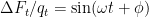 is simply
  , where
  ,
,  ,
, ![D=\frac{(1/\tau+i\omega)[\sin(\phi)-i\cos(\phi)]}{(1-\lambda_0f)/\tau+i\omega}\lambda_0](https://s0.wp.com/latex.php?latex=D%3D%5Cfrac%7B%281%2F%5Ctau%2Bi%5Comega%29%5B%5Csin%28%5Cphi%29-i%5Ccos%28%5Cphi%29%5D%7D%7B%281-%5Clambda_0f%29%2F%5Ctau%2Bi%5Comega%7D%5Clambda_0&bg=ffffff&fg=000&s=0&c=20201002) , and
, and  . This is true independently of whether the loop gain
  exceeds unity.
 the response to a sinusoid stimulus is itself a finite-amplitude sinusoid. This is true both for the circuit and for Monckton et al.’s model. In particular, the response for
  , where Monckton et al.’s Fig. 5 plot goes infinite, is a sinusoid whose magnitude when
  is only
  times the stimulus’s and lags it in phase by 45 degrees.
 the response sinusoid’s magnitude approaches infinity. Moreover, the stimulus and response polarities are the same just below
  but opposite just above it. This is no doubt where Lord Monckton got his impression that “voltage that was doing its best to become infinitely positive tries its best to become infinitely negative.”
 parameter as not part of the feedback makes a distinction without a difference to the equations), it is not true that “In the climate, however, no such reversal is physically possible.” In the real climate, of course, the departure
  from some reference temperature won’t become infinite, but neither will the circuit’s response voltage; in both cases the parameters that would dictate such results will in real life so change as no longer to require them.
 exhibit a reversal of the temperature-departure response
  with respect to the radiative stimulus, a reversal exactly analogous to the circuit output voltage’s reversal with respect to its input voltage.
 crosses unity. So one might think this tells us something about the response to a step stimulus, which some would characterize as a zero-frequency stimulus. But that would be incorrect, as my post demonstrated.
![\frac{\lambda_0\omega\cos(\phi)-(1-\lambda_0f)\sin(\phi)}{[(1-\lambda_0f)\omega]^2/\tau}\lambda_0e^{(\lambda_0f-1)t/\tau}](https://s0.wp.com/latex.php?latex=%5Cfrac%7B%5Clambda_0%5Comega%5Ccos%28%5Cphi%29-%281-%5Clambda_0f%29%5Csin%28%5Cphi%29%7D%7B%5B%281-%5Clambda_0f%29%5Comega%5D%5E2%2F%5Ctau%7D%5Clambda_0e%5E%7B%28%5Clambda_0f-1%29t%2F%5Ctau%7D&bg=ffffff&fg=000&s=0&c=20201002) : the homogeneous component is an exponential that dies out for
: the homogeneous component is an exponential that dies out for  .
. approaches unity from the left, that exponential eventually dies out. And, on the right, the direction in which it grows without bound is not indicated by Monckton et al.’s Fig. 5 plot but rather dictated by the phase of the sinusoid that starts at time zero.
Be that as it may, I have been spurred by Bernie Hutchins’ comments to look at the response of my post’s amplifier to sinusoidal signals and thereby have perhaps put my finger on how Lord Monckton has arrived at his erroneous view of circuit analysis. In any event, I will use this comment to memorialize the results and perhaps give Lord Monckton something to refer to in case he actually does consult experts on the specific objections that I and many others have raised.
Although I showed a differential amplifier, i.e., one that has an inverting input port, nothing depends on that feature, and it probably avoids confusion to apply a positive signal to a non-inverting port rather than a negative signal to an inverting port. Assuming such a simplification, the resultant circuit’s equations are exactly the same as Monckton et al.’s model with
In theory, that is, even with
So, what does that plot’s infinity mean? Rather less than it seems to. True, as the stimulus sinusoid’s frequency approaches zero for
To the extent that this is true of the circuit, though, it is also true of the climate model; the same equations govern, so the same outputs must result. Barring some difference in the equations that Lord Monckton has studiously avoided identifying (and his insisting on characterizing the
Despite what Lord Monckton imagines, the reason for not following “the Bode equation” blindly doesn’t lie in the distinction between circuits and climate. It lies in a factor common to both of them: there are limits. In the case of the amplifier circuit, the limit is the amplifier’s limited output range. In the case of the climate, it’s probably that the feedback becomes more negative as temperature rises. So long as the systems operate within regimes where the model equations apply, though, the climate model will indeed for
Even the low-frequency behavior just mentioned, moreover, does not mean what some may think. As was just observed, the output at low frequency does indeed switch from in phase to 180 degrees out of phase as the loop gain
The problem, both for the circuit and for the climate, is that the foregoing analysis holds only when the stimulus is a perfect sinusoid. Even if it were the same as a perfect sinusoid from some time zero onward but had been equal to zero at all times before, the response would differ from the perfect-sinusoid case in that it would include not only the sinusoidal component set forth above but also a “homogeneous” component equal to
No matter how closely
In short, the mathematics requires considerable interpretation, and care must therefore be taken in drawing inferences from it. Now, circuits are more likely to be fairly linear in the region of interest than the climate is, so there are indeed good reasons to be particularly careful in applying linear-systems techniques to the climate. But distinctions such as failure to “transit to the negative rail” are not among them.
Although I don’t know Lord Monckton, I’ve followed the debate for years. Lord Monckton is one of the most colorful, interesting, knowledgeable and well spoken commentator for the skeptic position. I have not always agreed with everything he says or writes, but I do respect him and admire him. One thing I do believe to be true about Lord Monckton is that he is honest. If he wrote he consulted certain experts, I believe that he did. You have written that you doubt this – which to me is falling back on skills you learned as a lawyer. It is a great court room tactic to begin by denigrating the opposing sides honesty before talking about specifics.
I can’t imagine Lord Monckton “outing” people who have helped him or agree with him on some fact without them agreeing to this and them also actually wanting to enter the “fray”. Because if he identifies them, it is possible that they would be harassed and attacked depending on where they work or even denied promotions. There is the movement from liberals and progressives to find ways of “punishing” skeptics. And skeptics have suffered in various ways due simply to not sharing a viewpoint.
Unfortunately, he is not. He e.g. claimed that the peer review of his model paper was ‘double blind’. It was not.
A little exert from Professor Lockwood’s recent conclusions
from the activity minima in the MM, the (unsigned) OSF falls
to about 1014 Wb, which should be compared to values around
1015 Wb at the peaks of recent solar cycles. Thus the Earth’s
residence times in fast or intermediate flows would be an order
of magnitude shorter in the MM than during recent solar cycles
and enhancements in mean solar wind speeds would therefore
be of order a tenth that in recent cycles, i.e. of order 25 km s−1, if
fast and slow solar wind speeds remained the same and changes
are all caused by variations in Earth’s residence times in such
flow regimes. Therefore we conclude that solar wind speeds
would be relatively uniform in theMM(between about 250 and
275 km s−1, i.e. roughly half the average seen in modern times).
The authors are grateful to many scientists for
Oh, I don’t doubt that he’s consulted experts at some point; indeed, I suspect I know who one of them is. I just don’t think he got input from them regarding the specifics of my post or understood them if he did. If he had gotten that input and understood it, his response would have been better.
We had no idea who the reviewers were, and the reviewers had no idea who we were. That is double-blind review.
Your second claim is most unusual. I know of no reputable journal that practices that, and the website of the Chinese journal you submitted to does not mention [or as far as I can see] support that the reviewer does not know the authors. You may wish to restate your ‘misspoken’ [I think that is the current euphemism] comment.
Mr Born says my response would have been “better” if I had agreed with his mistakes, of which there were many, as the head posting demonstrates.
BobG is very kind. One of those with whom I have discussed the Bode problem has indeed asked to be kept anonymous, because he wants his paper to be peer reviewed and published before anyone plays politics with his scientific research. I am content to wait till that important paper appears. It could be the silver bullet that slays the bloodsucking global-warming vampire.
Joe is quite correct in that his original circuit did not have to be a differential amplifier. It would have been much better if he avoided the (-) input. It does however offer me an opening to make the point that feedback is neither positive or negative according to whether a non-inverting (+) or an inverting (-) terminal is used for the feedback. Instead, everything that happens around the loop (gains, phase shifts) matters. My write-up from Nov. 2013 has several relevant examples of multiple inversions leading to positive feedback (the concept is VERY well understood):
http://electronotes.netfirms.com/EN219.pdf
As for a frequency-dependent feedback loop, if you start out with what you believe is pure positive feedback, any amplitude attenuation in the loop (or course) reduces the degree of positive feedback. Any phase shift will, initially, also reduce positive feedback. ENOUGH phase shift will make the feedback negative. (Joe’s low-pass feedback will have a max phase shift of 90 degrees however).
More alarming for EE’s is the case where (intentionally implemented) pure negative feedback starts to become less negative because of unintended phase shift. This can cause oscillations. Often such oscillations ARE in fact rail-to-rail ugly trapezoids (non-linear effects). And it matters not if you intended to input such frequencies or not, and you can’t just ignore them. Noise will always set them off.
On the other hand, this sort of oscillation need NOT be rail-to-rail (power supply limits may not matter). For example, if you hang a scope cable (a capacitor) on the output of a unity-gain op-amp “follower” it can set off oscillations because of the phase shift due to the probe capacitance (perhaps 100 pF) and the output resistance (perhaps 100 ohms) of the real op-amp. This can be up around, say, 3 MHz, and is a small superposition on the desired waveform. The waveform looks very “fuzzy”. The oscillation is small and does not get to the rails because the op-amp output can’t “slew” anywhere near fast enough (limited by dV/dt for a particular op-amp type).
Analog electronics is complicated in itself. At least it sits neatly on a lab bench!
Here are the frequency response (magnitudes) and the step responses for Joe’s circuit.
http://electronotes.netfirms.com/JB.jpg
I did make the input non-inverting, and set the two resistors equal (just to make an example). Thus the feedback gain from the resistors is 1/2 (for DC frequency, and for long time) so the response at these points is A/(1-A/2). The critical gain A for sign change is thus A=2.
In the figure, the top two panels are for A=1 so the DC and long-time gains are 2, 1 on the opposite ends. The middle two panels are for A=1.9 (still stable), and is similar except for much larger gains with feedback. If we try A=2.1, the gain should be -42. This is the frequency response MAGNITUDE (bottom left panel). But not the exponentially ramping step response!
Usually the freq. resp. is calculated as the product of all distances, from a frequency point on the j-omega axis, to each zero, divided by the corresponding product of distances to the poles. Thus unstable right-half-plane poles do not show – unless someone codes in an alarm. But the step response ramps up to warn us.
What happens at A=2 where 1-(1/2)*2 = 0? The first freq. resp. point (DC) gives a divide-by-zero error. The step response is a LINEAR ramp.
All makes sense.
Mr Born’s continuing failure to grasp the very simple point I am making about the inapplicability of the Bode system-gain equation to the climate seems to arise from one error and one misinterpretation on his part. The error was his assumption that a change in the altitude of the characteristic-emission surface consequent upon a radiative forcing would cause the temperature of that surface to change. No. As previously explained, under the assumption that insolation, emissivity and albedo are near-constant, so will the temperature of the characteristic-emission surface be constant.
The misinterpretation – commonplace, but wrong – is in his assumption that the Planck parameter is a feedback just like all the others. No. In fact, it plays a special role in the determination of climate sensitivity, is not summed with the true feedbacks but is, uniquely, instead multiplied by their sum, is separately multiplied by the initial forcing to determine zero-feedback warming, again unlike any of the true feedbacks, and is better expressed in Kelvin per Watt per square meter of forcing as part of the reference frame for the determination of climate sensitivity (see Roe, 2009, for a discussion).
So to his criticisms of those of us who question the applicability of the Bode system-gain equation, which he seems to believe is of universal applicability in dynamical systems. No. It was not designed for systems – such as the climate – in which the output (temperature change, in the climate) is the instrument by which the system self-equilibrates. Nor is it applicable to systems, such as the climate, in which the feedbacks do not cause a reversal in the direction of the output at a loop gain of unity. In an electronic circuit, the singularity in the Bode equation has a physical meaning, though even there it should be treated with caution. In the climate the singularity does not represent physical reality.
The matter is actually very simple. The Bode equation appears to suggest that at loop gains much above the process engineers’ rule-of-thumb design limit of 0.1 a very rapid amplification of the original perturbation occurs. In electronic circuits, that is indeed what happens, unless they have been specifically designed to act homeostatically and to resist feedback amplification.
The climate, on the other hand, is pronouncedly thermostatic, so that no curve remotely resembling the Bode equation at or near the singularity can apply. Yet in the models (see e.g. Hansen, 1988 for some worked examples) the equation is applied strictly, and without even making the obvious allowance for the fact that asymptotic upper and lower bounds on temperature change must apply, just as they must apply to an electronic circuit, in which generating an infinite voltage is not possible.
It is all very well for Mr Born to say airily that the input parameters would change to prevent climate sensitivities approaching infinity, but the modelers do not sufficiently change the parameters in their models to reflect the homeostatic real world.
Those worked examples, incidentally, demonstrate that the modelers apply the Bode equation naively to the direct warming to obtain the amplified warming. As so often, Mr Born should really be taking issue with them and not with me. They are applying the Bode equation in a fashion in which it cannot legitimately be applied. Mr Born has so far been silent on how they actually use the equation: it is in their manner of using it that climate sensitivity ends up being prodigiously exaggerated.
And, though Fourier analysis in the frequency domain is sometimes useful, in the present instance it is not really helpful.
Absurd papers such as Murphy (2009) claim that climate sensitivities of 10+ K are possible: but the sole reason for that conclusion is their misapplication of the Bode equation to an object to which – in its unmodified form – it simply does not apply.
Interestingly, on seeing our paper the climate extremists did not even attempt to suggest that there is nothing wrong with a strict application of the Bode system-gain equation to the climate. As soon as they saw the output curve, they realized that that curve does not apply to the climate. So, instead, one of them tried to deny that the equation is used in the models. He said, “I’m a GISS modeller: I know the equation is not used in our model.” But it is used in his model, though he had not realized this. And it is used in a fashion that is calculated to generate the absurdly high climate sensitivities that the output curve as it approaches the singularity would seem to suggest.
Another commenter – at the World Federation of Scientists’ annual conference two years ago – said that the equation works well enough up to a loop gain of 0.8 – which, conveniently, is the IPCC’s implicit upper bound on its central climate-sensitivity interval. However, it is likely that in the real world all values >>0.1 there should be a toning-down of the equation’s output.
Mr Born is entitled to his opinion that the voltage in an electronic circuit does not change direction at the singularity in the Bode equation: but, if he will put “feedback-induced oscillation” or “from the positive to the negative rail” into a search engine he may learn otherwise.
However, the central point is that the models do not at present adjust the Bode equation even to the extent of attempting to model the effect of the necessary asymptotes on the output of the equation not only at the singularity but also across quite a substantial interval either side of it. For this reason, among many others, they are prone to exaggerate climate sensitivity. Any reasonable correction of the Bode equation would cause climate sensitivity to fall by two-thirds to four-fifths.
That is why researchers far more versed in these matters than Mr Born or me have realized that the problem I have drawn to their attention is serious and requires attention. And, whether Mr Born likes it or not, they will now address the real problem that the Bode equation represents, a problem that has appeared previously in the literature, and – if current indications are confirmed – they will find climate sensitivity considerably lower than the overheated values currently in vogue.
Lord Monckton –
You wrote: ” but, if he will put “feedback-induced oscillation” or “from the positive to the negative rail” into a search engine he may learn otherwise.”
I tried both these on Google. Found nothing relevant – or so it seemed to me. Can you give actual links?
Lord Monckton. Addendum. The problem remains your saying:
“ Mr Born is entitled to his opinion that the voltage in an electronic circuit does not change direction at the singularity in the Bode equation: but, if he will put “feedback-induced oscillation” or “from the positive to the negative rail” into a search engine he may learn otherwise. ”
Searching with these terms leads mainly to OSCILLATORS. No one is suggesting that oscillators do not go negative (or at least become less positive), over and over in a cycle. That’s what an oscillator is all about. There are many MECHANISMS of achieving electrical oscillations going back more than 100 years.
Sitting exactly on the singularity of the Bode equation is one theoretical CONDITION to achieving oscillation. [In practice one must exceed that singularity ever so slightly, impose limiting (or rely on the limiting of power supply rails), and accept a small measure of harmonic distortion.] The Bode singularity is not a mechanism that causes the individual reversals. It is a condition that indicates the circuit polarity reversals can occur.
Is it possible that you are conflating the condition with the mechanism?
Joe’s circuit is first-order and not an oscillator (see my graphs above). Well – it does “oscillate” at DC – it is an integrator at the singularity. Its impulse response is a step. Its step response is a linear ramp (as I stated).
I am talking electronics here – nothing about climate. But I think we have to get the electronics (cowering on a lab bench) understood first.
All we need to do is understand how the Bode equation is actually used in climate models. It represents a physical reality in an electronic circuit; it does not represent a physical reality in the climate.
You said “It represents a physical reality in an electronic circuit; it does not represent a physical reality in the climate.”
Likely so. But, sorry to say, it appears you don’t understand the electronics.
It would be easier to instead note where the climate models have gone right, its a much shorter list, e.g. they spell “climate” correctly. Not sure there is anything else for this list.
Leif , your opinion is your opinion but apparently many do not agree with it.
Lockwood does as far as calculating V and B [his Figure 2]. He is finally admitting that I was right all along. This is a healthy development on his part.
http://www.leif.org/research/Lockwood-Agrees.png
I had not read any of Lockwood’s recent papers. However, out of curiosity, I read http://www.eiscat.rl.ac.uk/Members/mike/publications/pdfs/2014/308_OSF1_jgra51127.pdf
“5. Conclusions
We have studied the putative discontinuity in the international sunspot number record in around 1 January 1946. Our results confirm the conclusion of Svalgaard [2011] that the discontinuity is present in the widely used data set that is available from most data centers. However, Svalgaard’s estimate that a 20% correction is here shown to be an overestimate. Using the RGO/SOON spot area, Svalgaard [2011] actually found an 18% correction (it is not clear from his paper how this was quantified) that he rounded up to 20%, but both values are far out on the far tail of the probability distribution found here. We suggest preferred value should be based on sunspot data alone, maintaining its independence from geomagnetic data: we have demonstrated problems with early IDV data caused by a failure to maintain that independence. Hence, we recommend an optimum correction of 11.6%, with the 2σ uncertainty range being 8–14%. The geomagnetic data provide broad confirmation of this with IDV giving and optimum correction of 10.3% and IDV(1d) giving 7.9%. “
Lockwood is usually behind the curve with usually flawed papers and this one is no exception. He knows quite well [but pretends not to] that the Locarno sunspot overcount is determined by direct comparison between the weighted and unweighted sunspot counts, as explained here:
http://www.leif.org/research/Locarno-Overcount.png
But not to worry, give him a few years and he will catch up as he always does. It is just a pity that he carpet bombs the field with bad papers.
We disagree. Have a good night.
so, you disagree with Lockwood when he shows that he agrees with me? His Figure 2.
Now, probably we are both a bit wrong in the derivation of the solar wind speed [V]. The slow increase from 1870 until today is likely to be an artifact caused by not taking into account [we don’t precisely know how to] the decreasing main field of the Earth, which causes geomagnetic activity to be a bit higher than it should be for equal solar wind.
I say let us see how this prolonged solar minimum plays out before saying with 100% certainty this is how it is ,this is how it will be.
If this prolonged solar minimum becomes established going forward answers should be coming? At least I hope so.
Right now for me it is wait and see. I think unexpected scenarios will arise going forward. However ,I have no thought if it will favor any ones particular stance or not.
The more I look into this the more I feel that is not known rather then what is known. To much gray area is out there for my taste.
Would anyone care to explain what they mean by the phrase “global warming”?
Mike:
Thanks for taking the time to respond. How would one measure the “global warming” or is it, as I understand the issue, immeasurable?
Mike Borgelt
Electromagnetic energy, eh? Are you sure that’s not long wave thermal energy emitted from the earth into space?
Lord M: Grist for another of your mills:
Climatic Change
DOI 10.1007/s10584-015-1343-
“The social cost of atmospheric release” by Drew T. Shindell
http://download.springer.com/static/pdf/498/art%253A10.1007%252Fs10584-015-1343-0.pdf?auth66=1426965671_834f21d7c410f4d1f1bd3906430c9cce&ext=.pdf
His arguments are entirely based on a ‘high discount rate’. As you have shown several times, mitigation is much cheaper when the discount rate is high. A response from you to this paper would invite an animated discussion here. I look forward to it!