Guest essay by Joe Born
In Monckton et al., “Why Models Run Hot: Results from an Irreducibly Simple Climate Model,” the manner in which the authors used their so-called transience fraction raised questions in the minds of many readers. The discussion below tells why. It will show that the Monckton et al. paper obscures the various factors that should go into selecting that parameter, and it will suggest that the authors seem to have used it improperly. It will also explain why so many object to their discussion of electronic circuits.
The discussion below will not deal with how well the model performs or whether the Monckton et al. paper interpreted the IPCC reports correctly. It will be limited to basic feedback principles that are obvious to most engineers and to not a few scientists. But there are circumstances in which stating the obvious is helpful, and I believe that Monckton et al. have presented us one.
Equation 1 of the Monckton et al. paper provides us laymen with a handy back-of-the-envelope model by which we can perform sanity checks on things we hear about the climate system. If we concentrate on equilibrium values and assume that carbon dioxide is the only driver, we can drop the  ‘s from that equation’s penultimate line and take the
  and
and  parameters to be unity to obtain:
The expression on the right can be recognized as the solution to the equation illustrated by Fig. 1, namely,  .
.

Here  is a temperature-change response to the initial radiation imbalance
  , or “forcing,” that would result from a carbon-dioxide-concentration-caused optical-density increase. The optical-density increase raises the effective altitude—and, lapse rate being what it is, reduces the effective temperature—from which the earth radiates into space, so less heat escapes, and the earth warms. The
  ‘s represent departures from a hypothetical initial equilibrium state of zero net top-of-the-atmosphere radiation, and the forcing is considered to keep the same value so long as the increased carbon-dioxide concentration does, even if the consequent temperature increase has eliminated the initial radiation imbalance and thus returned the system to equilibrium.
Without any knock-on effects, or “feedback,” the response would simply be  , where
  is a coefficient widely accepted to be approximately 0.32
  . The forcing produced by a carbon-dioxide-concentration increase from
  to
to  is stated by the last line of Monckton et al.’s Equation 1 to be
  , where it is widely accepted that
  , i.e., that a doubling of the CO2 concentration would cause a forcing of about
  .
.
So the model’s user can readily see the significance of the main controversial parameter, namely, the feedback coefficient  , which represents knock-on effects such as those caused by the consequent increases in water vapor, the resultant reduction in lapse rate, etc. In particular, the user can see that if were positive enough to make
  close to unity—i.e., to make the right-hand-side expression’s denominator close to zero—the global temperature would be highly sensitive to small variations in various parameters.
Fig. 2 depicts this effect: approaches infinity as approaches 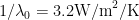 , i.e., as
  approaches unity. (That plot omits
  values that exceed unity; for reasons we discuss below, Monckton et al.’s discussion of that regime in connection with electronic circuits is questionable.)

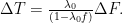
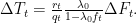
The quantities discussed so far are those that occur at equilibrium, i.e., in the condition that prevails after a given forcing has been constant for a long enough time that transient effects in the response have died out. To arrive at a value for times when the forcing has not been remained unchanged long enough to reach equilibrium, the model includes a “transience fraction” to represent the ratio that the response at time bears to the equilibrium value. Other subscript ‘s are added to indicate that for different times the various quantities’ effective values may differ. Finally, to arrive at the response to all forcings, a coefficient representing the ratio that carbon-dioxide forcing bears to all forcings is included:
As we mentioned above, the transience fraction is of particular interest. As the Monckton et al. paper’s Table 2 shows, the ratio that the response at time bears to its equilibrium value depends not only on time but also on the feedback coefficient . Of course, it would be too complicated for us to investigate how such a dependence arises in the climate models on which the IPCC depends. But we can get an inkling by so modifying the block diagram of Fig. 1 as to incorporate a simple “one-box” (single-pole) time dependence.
Fig. 3 depicts the resultant system. The bottom box bears the legend “ ,” which in some circles means that the rate at which that box’s output changes is the product of its input and a heat capacity
  . (The
  is the complex frequency of which Laplace transforms are functions, but we needn’t deal with that here; suffice it to say that division by in the complex-frequency domain corresponds to integration in the time domain.)
What the diagram says is that a sudden drop in the amount of radiation escaping into space causes the temperature response to rise as the integral of the stimulus divided by . That temperature rise both increases the radiation escape by  and partially offsets that radiation escape by
  .
.

Now, Fig. 3 can justly be criticized for wildly conflating time scales; it does not reflect the fact that the speed with which the surface temperature would respond to optical density alone is much greater than, say, the speed of feedback due to icecap-caused albedo changes. But that diagram is adequate to illustrate certain basic feedback principles.
The output of the Fig. 3 system is a solution to the following equation:

For example, if  equals zero before
  and it equals
  thereafter, that solution for
  is:
is:
where  . That is, the equilibrium value of
  is the same as it was before we added the time dependence, but the added time dependence shows that the equilibrium value is approached asymptotically.
Fig. 4 depicts the solution for several values of feedback coefficient . What it shows is that a greater feedback coefficient yields a higher temperature output .

Another way of looking at the response is to separate its shape from its amplitude, and that brings us to transience fraction , which is our principal focus. Fig. 5 depicts this quantity, which is the ratio at time of the response to its equilibrium value. That plot shows that, although greater feedback results in a greater equilibrium temperature, it also results in the equilibrium value’s being reached more slowly.

Of course, those plots give the relationship between current and equilibrium output only for our toy, one-box model. Monckton et al. instead employed the relationship set forth in their Table 2 and depicted by the dashed lines in Fig. 6 below. In a manner that their paper does not make entirely clear, they inferred the Table 2 relationship from a paper by Gerard Roe, who explored feedback and depicted in his Fig. 6 (similar to Monckton et al.’s Fig. 4) how a “simple advective-diffusive ocean model” responds to a step in forcing for various values of feedback coefficient.

As Fig. 6 above shows, the Monckton et al. values initially rise more quickly, but then approach unity more slowly, than the ones that result from our Fig. 3 one-box model. As to the specifics of his model, Roe merely referred to a pay-walled paper, but in light of his describing that model as having a “diffusive” aspect we might compare the Table 2 values with the behavior of, say, a semi-infinite slab’s surface, as Fig. 7 does. Except for the  value, the curves are similar over the illustrated time interval, but the slab thermal diffusivity used to generate Fig. 7’s solid curves was about 2000 times that of water, so the nature of the Roe model remains a mystery. Monckton et al. may have had a reason for following Roe’s model choice instead of any other, but they did not share that reason with their readers. For all we can tell, that choice was arbitrary.

More troubling, though, was the fact that they chose only a single transience-fraction curve for each value of total feedback, whereas we would expect that the curve would additionally depend on other factors. Let’s return to a simple lumped-parameter model like Fig. 3 to discuss what some of those factors may be.
Recall that in Fig. 3 the two feedback boxes were the same except for their values and  ; the feedbacks they represent did not operate over different time scales. But the IPCC models can be expected to employ feedbacks that operate with different delays. Feedback effects such as water vapor may act quickly, whereas the albedo effects of melting icecaps may become manifest only over long time intervals.
To illustrate such a difference, we divide the feedback represented by Fig. 3’s upper feedback box into two portions, as Fig. 8 illustrates:  and
and  ,
,  . The legend
  in the uppermost box means that its output asymptotically approaches times the input with a time constant of
  . In other words, if that box’s input were a step from zero to
  at time zero, its output would be
  at time .

Now we’ll compare the responses of Fig. 8-type systems that differ not only in feedback but also in the portion  of the feedback that operates with a greater delay. Fig. 9 compares such different systems’ responses, and we see that, as we expect, the magnitude of the higher-feedback system’s response is greater. In contrast to what we saw before, though, Fig. 10’s comparison of the systems’ curves shows that it is the higher-feedback system that responds more quickly. This tells us that the curve depends not only on the value of total feedback but also on the nature of that feedback’s particular constituents. And it raises the question of what feedback-speed mix Monckton et al. assumed.


Or maybe it raises the question of just how simple their model is to use. Let’s return to that model and note the dependencies on :
Of the five subscript ’s, three simply represent the time dependence of the stimulus or response, leaving the subscripts on the feedback coefficient  and transience fraction to represent the time dependence of the model itself. That equation might initially suggest a rather complicated relationship: transience fraction depends not only on time but also on the feedback coefficient—which itself depends on time.
But Monckton et al.’s Table 2 suggests that the relationship not quite as convoluted as all that: the transience fraction actually depends not on time-variant feedback but only on  , the value that the feedback coefficient reaches after all feedbacks have completely kicked in. One may therefore speculate that, although the transience-fraction function depends on the feedback’s ultimate value, that function was not intended to account for feedback time variation; one might speculate that the feedback time function serves that purpose.
But that would make the §4.8 discussion of the transience fraction puzzling, since it begins with the observation that “feedbacks act over varying timescales from decades to millennia” and goes on to explain that “the delay in the action of feedbacks and hence in surface temperature response to a given forcing is accounted for by the transience fraction .” So Monckton et al. did not make it clear just where the feedback’s time variation should go. Also, separating the feedback’s final value from its time variation in the manner we just considered doesn’t work out mathematically, particularly in the early years of the stimulus step.
And that brings us to another problem. Note that the forcing used as the stimulus by the Roe paper from which Monckton et al. obtained their Table 2 values was a step function: the forcing took a single step to a new value at and then maintained that value. That’s the type of stimulus we have tacitly assumed in the discussion so far. But the CO2 forcing in real life has been more of a ramp than a step, so we would expect the function to differ from what we have considered previously.
In Fig. 11 the dotted curves represent step and ramp stimuli, while the solid curves represent a common system’s corresponding curves. Obviously, the values are lower for the ramp response than for the step response.

For all that is apparent, though, Monckton et al. failed to make this distinction. In their §7 and Table 4 they appear to use the step-response values of their Table 2 to model the response to a forcing that rose between 1850 and the present, and that forcing was not a step; it was more like a ramp. The Table 2 values could have been used properly, of course, by convolving them with the forcing’s time derivative, but nothing in the Monckton et al. paper suggested employing such an approach—which, in any event, does not lend itself well to pocket-calculator implementation.
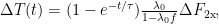
Moreover, it’s not clear how Monckton et al.’s §7 statement that “the 0.6 K committed but unrealized warming mentioned in AR4, AR5 is non-existent” was arrived at. That section refers to their Table 4, which shows that the values computed for the model result from multiplication by a transience fraction , supposedly taken from Table 2. The values 0.7, 0.6, and 0.5 respectively given in Table 4 for f values 1, 1.5, 2.2 suggest that in fact the central estimate leaves (1 – 1/0.6) * 0.8 = 0.53 K of warming yet to be realized.
So Monckton et al. have chosen a family of curves based on a model cited by Roe that for all they’ve explained is no better than the toy models of Figs. 3 and 8. Those curves apparently result from applying to that model a step stimulus rather than the more ramp-like stimulus that carbon-dioxide enrichment has caused. Although their discussion did refer to the fact that some feedbacks operate more slowly than others, they did not clearly tell where to incorporate the mix of feedback speeds to be assumed. And, as we just observed, it’s not clear that they properly used the transience-fraction curves they did choose in concluding that “the 0.6 K committed but unrealized warming mentioned in AR4, AR5 is non-existent.” In short, their selection and application of values are confusing.
That doesn’t mean that their model lacks utility. If one keeps in mind that various factors Monckton et al. do not discuss affect the curve, their model can afford insight into various effects that we laymen hear about. In particular, it can help us assess the plausibility of various claimed feedback levels. A particularly effective use of the model is set forth in their §8.1. If the authors’ representation of IPCC feedback estimates is correct, their model helps us laymen appreciate why the IPCC’s failure to reduce its equilibrium climate-sensitivity estimate requires explanation in the face of reduced feedback estimates. And note that §8.1 doesn’t depend on at all.
Despite the confusion caused by Monckton et al.’s discussion of , therefore, Monckton et al. have provided a handy way for us laymen to perform sanity checks. And their model helps us understand their reservations regarding the plausibility of significantly positive feedback. It shows that, generally speaking, one would expect high positive feedback to cause relatively wild swings, whereas the earth’s temperature has remained within a narrow range for hundreds of thousands of years.
Unfortunately, they compromised their argument’s force with an unnecessary discussion of electronics that did more to raise questions than to persuade. Specifically, their paper says:
“In Fig. 5, a regime of temperature stability is represented by  , the maximum value allowed by process engineers designing electronic circuits intended not to oscillate under any operating conditions.”
Although that lore may make sense in some contexts, it’s quite arbitrary; parasitic reactances and other effects can result in unintended oscillation even in amplifiers designed to employ negative values of  . Even worse is the following:
“Also, in electronic circuits, the singularity at  , where the voltage transits from the positive to the negative rail, has a physical meaning: in the climate, it has none.”
And Lord Monckton expanded upon that theme as follows
“Thus, in a circuit, the output (the voltage) becomes negative at loop gains >1.”
Although one can no doubt conjure up a situation in which such a result would eventuate, it’s hardly the inevitable consequence of greater-than-unity loop gains. To see this, consider the circuit of Fig. 12.

The amplifier in that drawing generates an output  that within the amplifier’s normal operating range equals the product of its open-loop gain
  and the difference between signals received at its inverting (-) and non-inverting (+) input ports. In the illustrated circuit the non-inverting input port receives a positive fraction of the output from a resistive voltage-divider network so that, in the absence of the capacitor, the non-inverting port’s input would be
  . A negative voltage at the inverting port would result in a positive output voltage, which, because it is positively fed back, would tend to make the output even more positive than the open-loop value
Now, that is not a particularly typical use of feedback. More typically feedback is designed to be negative because the open-loop gain undesirably depends on the input—i.e., the amplifier is nonlinear—yet for  (and typically is much, much larger than the value 5 we use below for purposes of explanation), the closed-loop gain
 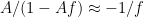 : the relationship
  is nearly linear despite the amplifier’s nonlinearity.
In principle, though, if is independent of input, there are no stray reactances to worry about, we are sure that the feedback coefficient will not change, the lark’s on the wing, etc., etc., then there is no reason why positive feedback cannot be used. If  and
and  , for example, the loop gain
  would be +0.5, which would make the output
  : that feedback would double the gain.
But in that example the loop gain is less than unity. What about  , which makes
  negative? I.e., what about the situation in which Monckton et al. tell us that “in a circuit, the output (the voltage) becomes negative”? Well, despite what they say, it doesn’t necessarily become negative.
To see that, let’s change the feedback coefficient to 0.4 and keep amplifier open-loop gain equal to 5 so that the loop gain  , i.e., so that the loop gain exceeds unity. And let’s make the inverting port’s input
  a time step from 0 volt to -0.1 volt. That value is inverted and amplified, the result appears as the output , and an attenuated version of that output appears at the non-inverting input port.
But propagation from output port to input port is not instantaneous, and, to enable us to observe what may happen during that propagation (and avoid tedious transmission-line math), we have exaggerated the inevitable time delay by placing a capacitor in the feedback circuit. (In a block diagram like those above, the legend on the feedback-circuit block would accordingly be  ).
).
As Fig. 13’s top plot shows, the output is initially (-0.1)(-5) = 0.5 volt and then rises exponentially as the feedback operates. If the amplifier had no limits, the output would grow without bound; despite what Monckton et al. say about in electronic circuits, the output would not go negative.
But we have assumed for Fig. 13 that the amplifier does have limits: its output is limited to less than 15 volts. Accordingly, the output goes no higher than 15 volts even though the signal at the non-inverting input port still increases for a time after the output reaches that limit. Still, the output does not go negative.

We could characterize that effect as the total loop gain’s decreasing to just under unity, as the middle plot illustrates, or as the small-signal loop gain’s falling abruptly to zero, which the bottom plot shows. (That is, no input change that doesn’t raise above +3 volts would result in any output change at all.) No matter how we characterize it, though, the  formula doesn’t apply in this case.
Why? Because it’s the solution to an equation 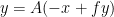 that says the output is equal to the product of (1) the amplifier gain and (2) the sum of the input
  and a fraction of the output. And in the
  case that equation is never true: delay prevents from ever catching up to
  until the amplifier gain has so decreased that the loop gain no longer exceeds unity.
Now, none of this contradicts Monckton et al.’s main point. Increasingly positive loop gains  make a system more sensitive to variations in parameters such as open-loop gain and feedback coefficient , so in light of the earth’s relatively narrow temperature range it’s unlikely that climate feedbacks are very positive—if they are positive at all. But the authors would have made their point more compellingly if they had avoided the circuit-theory discussion. And they would have made their model more accessible if their discussion of the transience fraction hadn’t raised so many questions.
Like this:
Like Loading...


“The optical-density increase raises the effective altitude—and, lapse rate being what it is, reduces the effective temperature—from which the earth radiates into space, so less heat escapes, and the earth warms.”
I look and I look and I have self-doubts but this just doesn’t make sense to me. The effective altitude of radiation is NOT set by the lapse rate. It is set by the ability to expel heat energy. As soon as that happens, whatever the altitude is, that is what it is. There is a missing ingredient in the explanation which is that while the altitude of effective emission has increased and the temperature at that altitude has decreased, there is MORE CO2 doing the radiating and the ability to radiate is permanently increased.
That this will self-stabilise is obvious. As soon as the more efficient radiator can dump the heat it will. The system is not depending on a less efficient radiator at a lower temperature, or a same-efficiency radiator, it is a more efficient radiator.
Combined with the thunderstorm transport system starting earlier in the day, the bypassing of the major portion of the atmosphere is easily and continuously accomplished.
Until the point is reached when thunderstorms would have to start before sunrise, to transport ‘additional heat’, we are going to see, on average, a remarkably stable temperature regime. Looking at the old behaviour that is going to be above 7000 ppm(v).
“Combined with the thunderstorm transport system starting earlier in the day, the bypassing of the major portion of the atmosphere is easily and continuously accomplished”
Nice model, and it makes the most sense to me. Feedback theory does not capture the chaotic feedback of this vertical heat transport.
“The effective altitude of radiation is NOT set by the lapse rate. It is set by the ability to expel heat energy.”
Well, I’m not a scientist; I’m just reporting what I think they think they’re modeling. But I believe you’re right that the lapse rate doesn’t set the effective radiation altitude. It’s the optical density; the lapse rate is what sets the temperature at the resultant altitude.
On the other hand, while it’s true that more carbon dioxide provides more radiators, it also provides more absorbers between those radiators and space. So the explanation I gave (well, regurgitated) seems plausible to me.
As to the ultimate result, I personally tend to agree with you that, encountering more resistance in the radiative path, more heat will be squeezed into the evaporative-convective path; latent heat will tunnel through the added resistance to become sensible heat where the optical path to space is shorter.
But, as I say, I’m no scientist; I’m just pointing out the logical issues that arise from the way Monckton et al. use their model. That is, if you compare a step-stimulus-derived output with ramp-stimulus-produced observations, the equilibrium value you infer is likely to be too low.
Joe Born March 13, 2015 at 6:53 am
“The effective altitude of radiation is NOT set by the lapse rate. It is set by the ability to expel heat energy.”
Well, I’m not a scientist; But, as I say, I’m no scientist;”
say that again, more loudly? I cannot hear you.
Perhaps the relationship between radiation, conduction, and convection is not properly accounted for, and their co-dependence is not properly modeled. Conduction and convection may lag radiation affects, but may also in time neutralize them.
“The optical-density increase raises the effective altitude—and, lapse rate being what it is, reduces the effective temperature—from which the earth radiates into space, so less heat escapes, and the earth warms.”
I look and I look and I have self-doubts but this just doesn’t make sense to me. The effective altitude of radiation is NOT set by the lapse rate. It is set by the ability to expel heat energy”
The ERL is set by the OPACITY of the atmosphere above it. Once the opacity reaches a low enough level
then the system can radiate freely to space. This opacity is fixed.
When you riase the amount of C02 the height at which this opacity is reached is raised.
how much has the “height” raised since 1950 Steven?
Can we actually measure that height? Or is it just a mathematical construct?
Steven – yeah we know that already and he says it above, but he was missing the part about there being more radiators. The difference in implication is simple enough: if the surface were heated by some other means, the altitude would rise ‘accordingly’. If the Cause of the increase is an increase in the mechanism by which heat is lost, then the altitude is reduced because it sheds heat more effectively. It goes up, but not nearly as much.
Any discussion of this model that does not mention transport of large amounts of heat vertically by thunderstorms is a diversion from the main task. Those thunderstorms have a concomitant cooling set of clouds to go with them.
So far it does not appear that the CO2 can get close to overpowering the negative feedback of the storms. Thermals beat thermalisation every time.
Good on you Steve.
Now explain to him how the amount of energy going out into space remains the same as before the CO2 increased.
Sure it is going out at a higher level with more CO2 in the air, and the air is warmer but there is no extra energy in the system because it all has to go back out, doesn’t it?
The air can be warmer but only at the expense of other layers being cooler.
Steven Mosher
March 13, 2015 at 2:00 pm
//////////////////////////////////////////////
Steven, your argument remains as inane as it ever was. You are essentially arguing that adding radiative gases to the atmosphere will reduce its radiative cooling ability.
It’s pointless arguing that if the IR opacity was 100% the surface average temp would be 255K. Empirical experiment proves this inane claim utterly false.
There’s no way out Steven. Every activist, journalist or politician who ever sough to promote or profit by this sorry hoax gets their public face, metaphorically speaking, punched to custard. You’re not up against sceptics any-more. The general public wants names. Sceptics know all the names….
When deriving a model whose purported purpose is to show “why the [CIMP] models run hot”, it seems perfectly reasonable to assume feedback effects whose time constants are large with respect to the time frame under consideration (a few decades) are constants folded into f. Also, I’m not sure why the author focused so much attention on the circuit analogy but his comparison seems apples-to-oranges. Lord Monckton confined his analogy to the region of stability with real (i.e. non-reactive) feedback while the author’s critic illustrates operation in an unstable regime with reactive feedback. Both conclusions are correct but about different things.
critic should read critique.
“When deriving a model whose purported purpose is to show “why the [CIMP] models run hot”, it seems perfectly reasonable to assume feedback effects whose time constants are large with respect to the time frame under consideration (a few decades) are constants folded into f.” and transience fraction is just what in some circles is called a step response. And, if
  is a constant, then transience fraction is just a normalized version of the step response. And that step response incorporates the feedback, including its reactive aspects.
The best way to implement the Monckton et al. is to make f a constant and use r_t to provide the time dependence, including the feedback delay. I didn’t show it here, but the choice of time function for f can be highly counter-intuitive if you try to put that time dependence into the f parameter. You can do it, but, instead of making the feedback coefficient grow gradually, you initially have to make it decrease gradually. Hardly what the pocket-calculator user would expect. So I’m guessing they used a constant f, which makes the subscript t on the f confusing.
“Also, I’m not sure why the author focused so much attention on the circuit analogy but his comparison seems apples-to-oranges.”
The reason for the circuit is that Lord Monckton often refers to electrical circuits, and he seems to think that the negative value for overall gain when the loop gain exceeds unity means that the voltage “transits to the negative rail.” He has often been called on that, but he doesn’t seem to understand the nature of the objection. This was my attempt to make him see it.
“Lord Monckton confined his analogy to the region of stability with real (i.e. non-reactive) feedback while the author’s critic illustrates operation in an unstable regime with reactive feedback.”
Although it’s true that the feedback values Monckton et al. listed in their Table 2 fell within the region of stability, my purpose was to respond to their statements about the lower-right region of their Fig.5, where they contrasted the its unphysical meaning for climate with what they contended is a physical meaning for circuits. Lord Monckton has said this kind of thing a lot, and he may benefit from understanding why he meets resistance when he does. So far he has defied enlightenment.
I’m not sure what you mean by the feedback’s being non-reactive; it operates with a delay.
Look, their product of
Joe,
Yes, I believe you’ve nailed it. Making f a time-dependent parameter overly complicates things and, to me, simply makes no sense.
If you don’t know of it, Knutti & Hegerl (2008) is a quite accessible general overview for estimating ECS: http://www.iac.ethz.ch/people/knuttir/papers/knutti08natgeo.pdf
I particularly like the Figure 1 cartoon, which steps through the immediate response to a forcing perturbation from near instantaneous all the way through to millennial-scale feedbacks, resulting in the “final” equilibrium response.
There are only two equations in the entire paper:
(1) ∆Q = ∆F – λ∆T, where λ = ∆F/∆T
(2) S = ∆T₀/(1 – f)
Quoting the paper: … where f is the feedback factor amplifying (if 0<f<1) or damping the initial blackbody response of ∆T₀ = 1.2°C for a CO2 doubling.
If I’m understanding the body of the paper correctly, I can write:
(3) ∆Q = ∆F – ∆T∆T₀/(1 – f)
Which is about as succinct a way to express net change in energy retained due to a change in atmospheric CO2 (or most any “well-mixed” GHG) concentration as I can conceive, and I believe the most “proper” way to think about it. Problem is, we don’t experience joules, we feel temperature. Same for large masses of landed ice.
Or course, the practical problems are that ∆Q eludes a complete accounting, f is not very well-constrained and ∆T is fiendishly difficult to tease apart from ∆T₀ observationally. ∆F is about the only thing in this model which I’d call all but bombproof.
I don’t think Monckton, et al. (2015) propose an irreducibly simple model for ECS with their two gain loops … they’re actually attempting to derive TCR, so of course they come up with a “models are too sensitive” conclusion. For ECS, the time-independent expression S = ∆T₀/(1 – f) should be sufficient, and so long as f < 1, process engineering best practices need not enter into the discussion.
There is also much confusion in these parts about f needing to be negative to “ensure” a stable system. MSLB (2015) mentions an oft-overlooked relevancy in their eq. (4): F = εσT^4
Were that also a linear relationship — or even approximately linear like most of what K&E (2008) are discussing — yes, I’m pretty sure all sorts of hell would break loose if f were anything BUT exactly dead zero.
Final note directed at the general audience here: the IPCC themselves say in AR5 that CMIP5 is likely 10% too hot.
And again, while Monckton was being sloppy, I think you are missing the point. For positive changes in temperature (voltage), the output of the model will go negative. To make the absurdity more apparent, the model will go to the opposite rail to the input signal sign. In the case of temperature (starting at ‘0’ at equilibrium), that means an increase in temperature will actually make the Earth freeze and a decrease in temperature will make the Earth roast. I would tend to call that pretty unphysical.
“I’m not sure what you mean by the feedback’s being non-reactive; it operates with a delay.”
Note the y-axis of his figure 6 is “Equilibrium Climate Sensitivity” so by implication the reference is to the _final value_ of the step-response of the system. By the final value theorem (in the limit as t->infinity, vo = vin * H(s) as s->0) reactive elements take on there DC values (caps become opens, inductors and series delays are shorts etc.)
“Look, their product of \lambda_\infty and transience fraction is just what in some circles is called a step response. And, if \lambda_\infty is a constant, then transience fraction is just a normalized version of the step response. And that step response incorporates the feedback, including its reactive aspects.”
This is incorrect. LM’s statement: “Bode mandates that at a closed-loop gain >1 feedbacks will act to reverse the system’s output. Thus, in a circuit, the output (the voltage) becomes negative at loop gains >1 ” is uncontroversial if in-artfully phrased (I would state that that loop gains >1 result in a phase reversal to cover both possible input polarities).
Again, by the final value theorem the ECS is just the transfer function (Laplace transform of the impulse response) of the system evaluated at s=0 (becase the s in the numerator introduced by the FVT is canceled when we integrate to get the step-response from the impulse response). In your (non) analogous circuit, the capacitor is inconsequential to the final value (it become an open) and thus to the analysis. In your circuit if f is the feedback fraction (f= R1/(R1+R2), Vof/X = A/(A*f-1) = A/(OLG-1), where Vof is the final voltage and OLG is the open loop gain. This system has an singularity at OLG = 1. Below that OLG value the denominator is negative and no phase inversion occurs (the sign of the output is the same as the sign of the feed-forward gain, in your case negative), above that value (non-physical region for real-world components) it’s positive and phase inversion occurs. As LM stated, this is a fundamental result of the Bode feedback formulation and the final value theorem. Are you really arguing that the Bode or FVT is wrong?
Jeff Patterson: “Again, by the final value theorem the ECS is just the transfer function (Laplace transform of the impulse response) of the system evaluated at s=0.” as set forth in one of the Table 2 rows the model’s response to a unit step? If not, what is it?
Believe me, I understand your difficulty; the same thing troubled me when I looked at this initially. But the experience I’ve had when I’ve dealt with experts in this area is that you have to be really careful about how you interpret the math, particularly when you’re dealing with feedback and/or complex numbers and/or taking limits. In those contexts, I’m told, you have to do a reality check.
Yes, if you apply a low-frequency signal, the output will blow up in the negative direction; I get that. But, as I said, you have to do a reality check when you’re taking limits.
So I did one, and the head-post analysis is what I got. There’s no mechanism I can identify that results in a simple step’s making that circuit’s output go negative. If you can identify one, I will be happy to be enlightened; I’ve been wrong before. But blindly following magic formulas doesn’t do it for me.
Jeff Patterson: “This is incorrect.”
Isn’t
Only Monckton’s conclusion is correct.
The other conclusion is drawn with so much waffle that no one here could understand the conclusions because they are riddled with assumptions and putting words into people’s mouths.
eg
“More troubling, though, was the fact that they chose only a single transience-fraction curve for each value of total feedback, whereas we [read Joe Born] would expect that the curve would additionally depend on other factors.”
They chose a simple single transience-fraction curve, Joe, to input into a simple model.
Which by the way works.
Why do you not congratulate him for this?
”Why do you not congratulate him for this?”
Still not getting it? Because Monckton is wrong. Adding radiative gases to the atmosphere will not reduce the atmosphere’s radiative cooling ability.
You are a warmist and therefore a scientifically illiterate socialist. What does it matter to true sceptics if Monckton the fool plays his “warming but less than we thought” games? Nothing. You are a collectivist. You cannot understand. This is not about left or right. This is not about “sides”. This is about right or wrong.
In defeat, it is no good trying to side with the foolish and wet “sceptics” that are most favourable to your failed cause. This is not politics. This is science. You came to a science fight armed only with propaganda. Your Alinsky techniques are powerless here. Right or wrong. Black or white. There is no “nuance”.
Your political games can never work. You seek to align sceptics behind the ludicrous lukewarmers? Bwahahahaha…
Herding sceptics would like trying to herd cats. You are not going to win. Not now. Not ever.
Konrad says:
You are a warmist and therefore a scientifically illiterate socialist.
C’mon, Konrad, that doesn’t necessarily follow. And then you added the comment about herding skeptics? I agree with that one. But it sort of contradicts what you said above.
Also, LM may or may not be wrong. I don’t know in this case. But he is not a fool.
dbstealey,
I disagree with K-rad on many things, but his mockery of WUWT’s closet Slayers for lapping up Monckton, et al. (2015) isn’t one of them. They tow the IPCC party line on the theoretical basis almost 100%, the main difference is in application and conclusion, which hinges on the notion that no engineer in their right mind would design a system with a closed-loop feedback gain > 0.1 if stability were the goal. That’s the kind of thing which has no business being presented as an a priori in an empirical physical science. A working assumption to develop a hypothesis, sure. A basis for conclusion, no. As you ironically say, it does not necessarily follow. The maths are that the system will be stable so long as closed-loop feedback gain is < 1. Monckton and crew are rightfully mocked to argue otherwise.
I am afraid I don’t see the point of this. Why should climate behave like an electric circuit? Is there any justification for the idea?
The point of simple energy balance models is right there is the name: they are simple and they are based on a fundamental physical principle, the conservation of energy. Those are very useful characteristics that make such models worthwhile in spite of their not representing anything close to the complexity of the climate system.
Proper climate models start with the same principles but distribute the energy among many “boxes” rather than one big box and, to the extent possible, use basic physical laws, such as those governing radiative energy transfer and fluid flow, to constrain the flows of energy. The result still leaves much to be desired, but at least it is a physics based attempt to make the model more realistic.
But this electric circuit business adds complexity with no reason, at least that I can see, to believe that the result is any more realistic. It may well be less realistic. So what is the point?
Electric circuits are wonderful. They are easy to build and test. They are amenable to mathematical analysis because it’s really easy (relatively) to isolate variables. That means that people doing systems analysis probably learned their math in circuits class.
At its heart, the argument about CAGW is an argument about feedbacks. Without feedbacks, a doubling of carbon dioxide will increase the planet’s temperature by a little more than one degree C. Positive feedback is required to get warming which would be catastrophic.
How could you prove that positive feedback existed (or not) in the climate system? You could try to use the math you learned in circuits class. If you do that, you’re making (whether you realize it or not) a bunch of simplifying assumptions. The problem is that we simply don’t understand the climate system well enough to know which simplifying assumptions are valid.
Au contraire, it’s actually an attempt to simplify the problem … believe it or not.
“Au contraire, it’s actually an attempt to simplify the problem”
For every complex problem there is an answer that is clear, simple, and wrong – H. L. Mencken
In my EE classes we started out by changing electronic circuit elements in to physical entities, e.g. resistors behave like dashpots (ideally, something where friction is proportional to velocity), inductors behave like masses, and capacitors behave like springs. So it’s easy to visualize an oscillating system made out of a weight and a spring. Add a dashpot and you can talk about car suspension systems.
You pretty quickly get to a point where it’s easier to just deal in electrical terms. After all, it’s easier to change a resistor in an oscillating circuit than to use an adjustable shock absorber. With active elements, it’s easy to add an amplifier to a circuit than to add a governor to an motor drive.
Ultimately, it becomes easier to design mechanical systems by first emulating them as electrical circuits and then build the mechanical system.
Mike M. March 13, 2015 at 9:00 am
I am afraid I don’t see the point of this. Why should climate behave like an electric circuit? Is there any justification for the idea?
Back in the day such simulations were called analog computers, in the 60’s they were better for modeling simultaneous differential equation networks than digital computers. The flight simulator used for the moon landings was an analog computer.
I teach a lab class where I use an integrated circuit system to demonstrate how negative and positive feedback can interact to cause oscillations, following that we set up a biological system where e.coli show oscillations in the same way. It’s a lot easier to control the oscillations in the electrical circuit than in the culture.
Phil,
One of my fellow grad students used an analog computer to solve a complex chemical kinetics problem represented by a set of stiff differential equations. But it was mathematically demonstrable that the system of differential equations governing the output of the analog computer was the same as the system of differential equations governing the kinetics model.
Such a demonstration is lacking here.
Guess my comment was redundant .
Yes m, my thesis was related to kinetic equations, particularly ‘stiff’ sets. We did some work with an analog computer which was much faster than the digital simulations, so you could use it to get a good feel of what the changes in parameters would do before doing the calculations.
But it was mathematically demonstrable that the system of differential equations governing the output of the analog computer was the same as the system of differential equations governing the kinetics model.
Such a demonstration is lacking here.
It should be possible to make such a demonstration for Monckton’s model.
I am way over my head here, because I have forgotten most of what I learned, when I was in school a very long time ago. Our Electrical Engineering department obtained a new EIA Pacer hybrid computer, and we got to play with it. The digital computer part controled the analog computer part, and I was told that Boeing used the same computer??? to design their wings and test them out, since it was too hard to directly solve the math equations for air flow. Additionally, all the Physics classes I sat through, watching the professors derive equations for the laws of Physics, left me with the impression, that you could write equations, but you couldn’t solve them, unless you knew what terms were trivial enough in the real world, that you could throw out and simplify the equations enough, so that they were solvable. So, maybe there is some merit in using the circuit/analog computer approach for climate modeling??? The equations must be at least as difficult (probably a lot more difficult), than the equations for airflow around a wing section. Just a thought.
Dan Sage
Old enough to remember analog computers ?
They were ( are ) just electrical circuits of op amps plugboarded to implement any sufficiently simple diff eq .
noone has successfully modelled the climate as a circuit.
its a bad metaphor
…..but great mental masturbation.
Judith Curry’s “Stadium Waves” don’t count?
Lots of things are like electric circuits! Water is a great analogy for electric flow in many cases. Water circuits can have feedbacks amplification too. My father worked with water based programming in the 60’s from an applications point of view. There were cards a little bigger than a credit card with circuits carved into them. They were analogue computer circuits as I recall.
The field of fluidics includes digital elements. My father experimented with some devices as they came out in the 60s, he brought a sample RS flipflop home to show me and experiment with. It was a lot like the bistable flipflop described in http://cad.uthm.edu.my/wisdom/courseware/FluidPower2003/chapter12/Chap12.5.html
Control Theory doesn’t care if you’re talking about an electric circuit or a flywheel engine or a waterwheel. It happens to be easy to build circuits that are a 1:1 map of any of those systems and so many times people will talk about the problem that way, but exactly the same rules apply to all feedback systems whether they use electrons or not.
Mike M. asks why the climate should behave like an electronic circuit. The point made in Monckton et al. is that there are several classes of dynamical systems, and the Bode system-gain equation that the climate models borrow from electronic circuitry and use as the pretext for multiplying the small direct warming from CO2 by 3, 5 or even 10 is not applicable to the class of dynamical systems in which the climate falls.
I believe both the author and Monckton are using simplified, linearized equations in place of the real nonlinear equations for the systems under discussion. Radiative heat transfer through a translucent material (the atmosphere) is governed by a system most accurately described nonlinear equation — not the simplified stuff above. Use of the linearized equations leads to incorrect, non-physical results — and endless arguments when two groups differ in their interpretation of which incorrect equation to use.
—- a system most accurately described by a nonlinear equation —-
The appendix to our paper provides the relevant equation for non-linear feedbacks. Furthermore, our time-series for the transience fraction is non-linear.
Monckton of Brenchley: “[O]ur time-series for the transience fraction is non-linear.”
Perhaps Mr. Hansen was referring to the models defined by the Table 2 transience-fraction functions, not to whether the transience fraction is a linear function function of time. Linear systems, of course, routinely produce outputs that are non-linear functions of time.
“I believe both the author and Monckton are using simplified, linearized equations in place of the real nonlinear equations for the systems under discussion.”
Then perhaps you should work on your reading comprehension. I wasn’t using linearized equations; I was showing that, to the extent that using them has utility, Monckton et al. used them incorrectly.
If you compare your model’s step response to the climate’s response to something more like a ramp, you’re doing something wrong. If your model says that the observed temperature increment is only 60% of what your model says the equilibrium value will be but conclude there’s no warming in the pipeline, you’re doing something wrong.
No one believes that the climate is linear. Its nonlinearity is not the news flash you perhaps believe. But many do believe that studying how feedback works in linear systems, which are much easier to compute, may give insight into what we might expect in non-linear ones. To the extent that they are correct, they should use those techniques correctly.
Monckton et al. didn’t.
.
Reply to Joe Born ==> Don’t get me wrong, I enjoyed your piece about the Monckton et al application — I was just pointing out something that is obvious but often needs to be pointed out over and over lest people begin to believe that the linearized climate models (or linearized models of any real world dynamical systems) can inform us of anything approaching reality, when the results are important. Two people using the wrong equations to find wrong results don’t make a right. Or, to put it another way, using the wrong equations the right way to correct the incorrect use of the wrong equations doesn’t arrive at the right or accurate answer either.
As you undoubtedly already know, the behavior of a nonlinear systems can be entirely different than that of its linearized analog. The fact the Monckton repeats the common error incorrectly, in your opinion, does not make repeating the error ‘correctly’ any more accurate.
Linearized analogs for dynamical systems do have some uses…arguing about the possible uses of them to model, however inaccurately, the climate system seems to be the most popular.
When we’re just fooling around, doing back-of-the-envelope sketches, thinking out an idea — they are adequate but can leave us with our behinds hanging out if we make the mistake of believing the results so obtained. No matter how many times your fuselage design passes through your Computational Fluid Dynamics (CFD) software, don’t fly an airplane design that hasn’t passed actual wind tunnel tests — which is where the unexpected, unpredicted turbulence brought on by the nonlinearities in the real fluid flow dynamics equations shakes your new design apart.
“Then perhaps you should work on your reading comprehension.”
What a great throw away line.
Perhaps you should work on your understanding of English.
Another great throwaway line.
” I wasn’t using linearized equations; I was showing that, to the extent that using them has utility,”
So you were using them mate, only he did it first.
This continual attack on Monckton, using semantics instead of real, provable arguments is disgusting.
Furthermore,
“If you compare your model’s step response to the climate’s response to something more like a ramp, you’re doing something wrong.”
Models are allowed to have steps in, it’s called data entry.
Steps have little lines drawn between them, this makes them into a a linear representation.
virtually all measurement is broken into steps or ramps if you focus in with a microscope./
“If you compare your model’s step response to the climate’s response to something more like a ramp, you’re doing something wrong.”
No you are the one breaking a simple argument down so far to where error can occur, on a microscopic scale.
But if a microscopic error is your reason for existence go for it
My detailed reply to Mr Born, once it is posted, will demonstrate that he, not I, is in error. For instance, since we consider temperature feedbacks to be net-negative, and since our model calculates that on assumption that all warming since 1850 was anthropogenic precisely the warming that has occurred should have occurred, it follows that there is no warming in the pipeline as a result of our past sins of emission.
Contrary to Mr Born’s assertion in the head posting, all of this is carefully explained in our paper: see, e.g., Table 4.
Actually, I’m assuming that I have indeed misinterpreted Table 4; I’d just like someone to explain where I went wrong.
In particular, I infer from the fact that Table 4’s third-last column was arrived at by multiplying by an r_t of 0.6 that 40% of the response remains to be seen. I also infer from Monckton et al.’s statement that no warming is left in the pipeline that my interpretation of Table 4 is somehow erroneous. But I’ve yet to see how.
An explanation would be helpful.
Joe Born –
“Still, the output does not go negative.”
I have not looked too deeply into the paper, and may be interpreting things inappropriately. However, is it possible that the case of loop gain > 1 is in the context of the system being embedded within a greater system with dominant negative feedback enforcing stability?
As a simple example, I could have a transfer function
1/(s – a)
with a greater than zero, embedded within an outer loop with feedback b, such that the entire transfer function is
1/(s -a + b)
This entire system would be stable if b is greater than a, and if you checked the output of the 1/(s-a) block versus its input, it would indeed invert it.
Forgive me if you already know everything in the following preface, but I don’t recall all my interlocutors. , radiative feedback, which exceeds the net of the other feedbacks to the extent that the net is positive: the overall feedback is negative, and I doubt that there’s any serious disagreement about that.
Actually, the loop gain > 1 discussion merely concerns a gratuitous comment by Monckton et al.–but one Lord Monckton often engages in, at the expense of his credibility in the eyes of those who know this stuff–regarding the difference between electrical circuits and the climate. Certainly there are differences, but the one he asserts isn’t among them. That was the only reason for the circuit discussion: Lord Monckton should abandon that branch of his argument.
With regard to feedback in the actual climate, Lord Monckton confines himself to loop gains less than unity–which is why the electrical-circuit distinction is gratuitous as well as wrong. The “positive” feedback usually discussed in climate circles is exclusive of the
Now, just in case that hasn’t made your question moot in your view, the answer is, Yes, feedback can turn a positive pole into a negative one. If the open-loop transfer function is 1 / (s – a), then negative feedback of magnitude f will make the overall transfer function 1 / (s – a + f), which puts the pole in the left half plane if f > a.
But I’m not sure where that fits into the discussion; I probably misunderstood your question.
“The “positive” feedback usually discussed in climate circles is exclusive of the -1/\lambda_0, radiative feedback, which exceeds the net of the other feedbacks to the extent that the net is positive: the overall feedback is negative, and I doubt that there’s any serious disagreement about that.”
English needed.
This is really the joke form of “all models are wrong, some models are useful”
Electron: “Are you sure about that?”
Positron: “I’m positive.”
Mr Born says he “knows this stuff” and implies that we don’t. As will be seen when my full response is posted, his assumption in this regard is incorrect. The reciprocal of the Planck parameter is not a temperature feedback, but is part of the reference frame within which all the true feedbacks operate. See Roe (2009) for a discussion.
The high-end estimates of feedback values in several IPCC reports, if taken together, would indeed exceed 3.2 Watts per square meter per Kelvin, implying a loop gain exceeding unity. Ross McKitrick made this point in a recent lecture. So this is no mere theoretical matter.
Mr Born says I should abandon this branch of my argument. Fortunately, it has now been taken up by one of the world’s top six experts on the application of feedback mathematics to the climate object, who has concluded that there is indeed a serious problem with the application of the Bode equation to the climate. He has also concluded that in consequence climate sensitivity cannot exceed 1 K and may well prove to be less. His paper saying so is out for review at present. Mr Born will then have the opportunity of submitting an attempted refutation of the Professor’s math to the relevant journal.
“But I’m not sure where that fits into the discussion…”
If that is the case, then it probably doesn’t. As I said, I have only glanced at the material in question.
I would caution against this, however:
“The “positive” feedback usually discussed in climate circles is exclusive of the -1/\lambda_0, radiative feedback, which exceeds the net of the other feedbacks to the extent that the net is positive: the overall feedback is negative, and I doubt that there’s any serious disagreement about that.”
It is not, in general, true that even an effectively unbounded negative feedback in one portion of the system confers stability on the system as a whole. For example, the system
dx/dt = -a*x + b*y
dy/dt = c*x
is unstable for a, b, and c positive, no matter how large a is. Such a system description is of importance in the climate debate. If x is temperature T and y is CO2, and the sensitivity b of temperature change to CO2 is positive, and sensitivity c of CO2 to temperature is positive, then the system would be unstable.
“It is not, in general, true that even an effectively unbounded negative feedback in one portion of the system confers stability on the system as a whole.”
Indeed. I should have specified that by “feedbacks” in “net of the feedbacks” I meant the different feedback paths’ respective DC gains. In your example, of course, one feedback path has an origin pole so that its DC gain is unbounded. The net would therefore not be negative.
But I would think that the rate at which the oceans emit carbon dioxide is more like proportional to the difference between the current atmospheric concentration and the equilibrium atmospheric concentration for the current ocean temperature. If so–and I’m no scientist, so don’t take my word for this–that particular feedback path would indeed be bounded; its pole would be in the left half plane, not on the origin.
Monckton of Brenchley: “Mr Born says he “knows this stuff” and implies that we don’t.”
I apologize if I seemed to imply that my knowledge in the area is superior to Monckton et al.’s; certainly, my modest credentials don’t compare to his colleagues’. Unfortunately, I was forced during my working life to operate extensively in fact situations where others’ expertise far exceeded mine, so I can assure you that I have come honestly by my modesty regarding any possible scientific or mathematical expertise.
Still, I like to think that my trade did give me a passable ability to recognize a good argument, and I have not yet seen one in Lord Monckton’s discussion of Bode equations.
Monckton of Brenchley: “Fortunately, it has now been taken up by one of the world’s top six experts on the application of feedback mathematics to the climate object, who has concluded that there is indeed a serious problem with the application of the Bode equation to the climate.”
I have no doubt that a good argument for that proposition can be made, and I await it with interest. My objection is only that making it with statements like “the voltage transits from the positive to the negative rail” generates heat but no light.
Joe Born @ur momisugly March 15, 2015 at 5:48 am
“But I would think that the rate at which the oceans emit carbon dioxide is more like proportional to the difference between the current atmospheric concentration and the equilibrium atmospheric concentration for the current ocean temperature.”
That makes
dCO2/dt = f(T)
for some function f(). A first order Taylor series expansion then results in
dCO2/dt = f(T0) + k*(T – T0)
where k is the partial derivative of f(T) evaluated at T0. If we are starting at some equilibrium point T0, then f(T0) = 0, and
dCO2/dt = k*(T – T0)
and, that is in fact what is observed:
http://www.woodfortrees.org/plot/esrl-co2/from:1979/mean:12/derivative/plot/uah/from:1959/scale:0.22/offset:0.14
“In your example, of course, one feedback path has an origin pole so that its DC gain is unbounded.”
Please note that the system
dx/dt = -a*x + b*y
dy/dt = -d*y + c*x
has apparent negative feedback in both paths, but this system is still unstable unless a*d-b*c is greater than zero. So, not only would the rate of removal of y have to be non-zero, it would have to be substantially so to produce a stable, well-behaved system.
But, if the rate of removal of CO2 were substantial, there would be no AGW debate. Something’s got to give. The aggregate response of temperatures to CO2 must be negligible in the present climate state. There is no way around it that I can see.
Bart: “dCO2/dt = k*(T – T0)”
That should be dCO2/dt = k_2 * (k*(T – T0) – CO2)
The k * (T – T0) is the equilibrium CO2 concentration, which CO2 tries to reach.
That makes it essentially the top feedback path in my Fig. 8.
As to your last comment, I’m sorry, but I didn’t understand where those equations came from, and they seem to reduce to a single second-order homogeneous equation in either of the variables. Can you explain that a little more?
Joe Born @ur momisugly March 15, 2015 at 5:36 pm
“That should be dCO2/dt = k_2 * (k*(T – T0) – CO2)”
That equation is incompatible with significant accumulation of CO2 in the atmosphere for significant k_2. Indeed, if there is a feedback of CO2 in this manner, it is very small. It hasn’t been observable in 57 years.
I started with x and y just to have a starting point of agreement. If you agree that
dx/dt = -a*x + b*y
dy/dt = -d*y + c*x
is unstable for a*c-b*d less than zero, then we can move on to applying it to the climate variables of interest.
The time evolution of absolute T, call it Tabs, should be something like
dTabs/dt = -alpha*Tabs^4 + beta(GHG)*S
where alpha is essentially emissivity times SB constant divided by heat capacity, beta(GHG) is a function of albedo and greenhouse gases, and S is solar forcing.
Define the temperature anomaly as T = Tabs – Teq, for some baseline temperature Teq. Let a = 4*alpha*T0^3, and b = partial derivative of beta(GHG)*S with respect to CO2 relative to some equilibrium level CO2eq such that a*Teq+b*CO2eq = 0. We have
dT/dt := -a*T + b*CO2
It is observed that
dCO2/dt = k*(T – T0)
but T0 is an arbitrary baseline, and we can easily redefine the baseline and CO2eq such that, substituting a constant c = k, we have
dT/dt = -a*T + b*CO2
dCO2/dt = c*T
which is exactly the form of the (x,y) system above.
If you want to tack on an unobserved feedback term such that
dCO2/dt = c*T – d*CO2
you just have to realize that A) the d term is too small to be discernible in the data of the last 57 years and B) that a significant d would not allow even human inputs to accumulate.
There is more I could add at this point, which would model the human inputs and elucidate how and why they could have negligible impact. But, I think this is probably a good stopping point for now, until and if you feel inclined to ask for more.
Bart: “If you agree that
dx/dt = -a*x + b*y
dy/dt = -d*y + c*x
is unstable for a*c-b*d less than zero, then we can move on to applying it to the climate variables of interest.”
Actually, I would have thought the stability criterion to be ad – bc > 0, but let’s move on anyway; I’ll re-check my math later.
My real problem lies in your equation dCO2/dt = k*(T – T0). Let’s say for the moment that T > T0 and we have a way to keep T constant; say we set a and b to zero temporarily. What that equation then says is that the CO2 concentration would increase without bound despite everything else’s staying the same.
Is that really what you intend to say?
“Actually, I would have thought the stability criterion to be ad – bc > 0…”
Yes, that is why it would be unstable for the opposite condition, as I stated.
“What that equation then says is that the CO2 concentration would increase without bound despite everything else’s staying the same. “
Well, yeah. Any differential equation dx/dt = f(x) will increase without bound if you keep f(x) constant but incongruently allow x to change. That’s a bit of a trivial observation, but it is essentially the same as what you have stated. If, however, I take the set of equations
dT/dt = -a*T + b*CO2
dCO2/dt = c*T
and set b negative with a and c positive, then the system will be stable. If I set b to zero, and add a small d such that
dT/dt = -a*T
dCO2/dt = c*T – d*CO2
then the system will be stable. Here is another stable configuration:
dT/dt = -a*T + b*CO2 – e*F
dCO2/dt = c*T
dF/dt = g*T
This set of equations can be simplified to
dT/dt = -a*T + G
dG/dt = (b*c-e*g)*T
where G = b*CO2 – e*F. This system is stable if b*c-e*g is less than or equal to zero. F is other ameliorative feedback from, e.g., cloud cover, or convective exchange of surface heat with atmospheric greenhouse gases which radiate the convected heat away.
The problem with the AGW hypothesis is that it has taken it as axiomatic that b is greater than zero, and there are no countervailing processes. While it is true that, all things being equal, the radiative imbalance induced by increasing CO2 should increase T, it is by no means assured that it will do so when all interactions are taken into account. The aggregate response to increasing CO2 must be stable, or we would not be here to question it.
And thats all –
some 2, 3 variables, ‘my’ variables,
condensed to constants, ‘my’ preferred constants’:
here ‘my’ preferred feedback loops!
a comic /a silent movie/ + ‘cascadeurs’ + sounds:
not even a picture of the world – but able to take it’s breath.
We’ve come a long way. Hans
Thanks Mr.Monckton, Joe Born, WUWT for clearing sight.
Hans
Joe Born, in your comment at 3:09am this morning, you stated that you had not performed a steady state analysis on your op amp model and that it was not germane to the discussion about Lord Monckton. I do not understand why. Could you expand on that part of the analysis for us?
The reason it wasn’t germane is that the step response was adequate to show why the “transit” doesn’t necessarily occur.
Frankly, though, I wanted to avoid the confusion that inevitably results from such discussions. The fact is that the g > 1 regime does in fact have a meaning when you’re dealing with frequency response, but it requires more interpretation than I cared to spend the time trying to express correctly.
The bottom line, though, is that, to the extent that models such as Monckton et al.’s apply to the climate, the interpretation that part of the graph has for electric circuits is precisely the same as it has for the climate. Of course, we can argue all day about the differences between electric circuits and the climate, but in my opinion Lord Monckton would be well-advised to drop this part of his argument, which is unnecessary and unnecessarily draws criticism.
I have prepared a detailed reply to Mr Born’s commentary on our paper, which I am hoping Anthony will publish shortly.
Monckton of Brenchley, I am unable to get to a copy of your paper from the link at the very beginning of this page. Is it accessible anywhere?
http://wmbriggs.com/public/Monckton.et.al.pdf
Thanks, Joe
Major Portions in Climate Change: Physical Approach by Kauppinen et al. (2011) also has RC-circuit analogy for the climate system. The paper is available at http://butler.cc.tut.fi/~trantala/opetus/files/FS-1550.Fysiikan.seminaari/Fileita/KauppinenJ-IREPHY-21Nov13.pdf
Thanks a lot for the link.
Although I generally agree with many of my (and Lord Monckton’s) critics that the these linear models’ limitations are severe, I believe they can afford some insight if one exercises judgment in using them. To that end, having at my fingertips the parameters provided by that paper will be helpful.
Thanks again.
3.7K per doubling? Curry and Lewis found it to be about 1.35K as a central estimate. This is vastly different. There is, btw, not enough accessible fossil fuel in the world to achieve such a doubling. Arrant nonsense.