
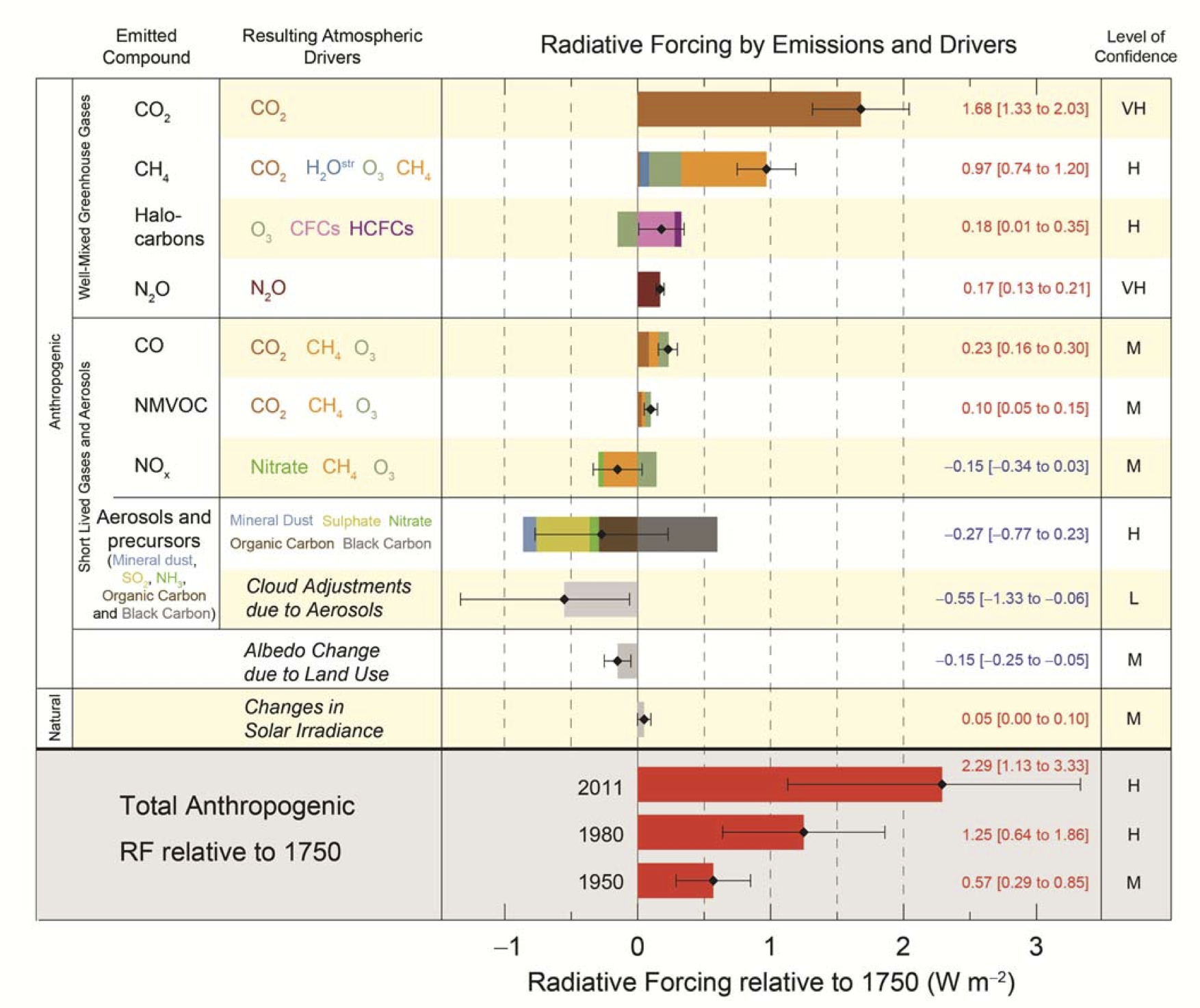
It was just yesterday that we highlighted this unrealistic claim from CMIP5 models: Laughable modeling study claims: in the middle of ‘the pause’, ‘climate is starting to change faster’. Now it seems that there is a major flaw in how the CMIP5 models treat incoming solar radiation, causing up to 30 Watts per square meter of spurious variations. To give you an idea of just how much of an error that is, the radiative forcing claimed to exist from carbon dioxide increases is said to be about 1.68 watts per square meter, a value about 18 times smaller than the error in the CMIP5 models!
The HockeySchtick writes:
New paper finds large calculation errors of solar radiation at the top of the atmosphere in climate models
A new paper published in Geophysical Research Letters finds astonishingly large errors in the most widely used ‘state of the art’ climate models due to incorrect calculation of solar radiation and the solar zenith angle at the top of the atmosphere.
According to the authors,
Annual incident solar radiation at the top of atmosphere (TOA) should be independent of longitudes. However, in many Coupled Model Intercomparison Project phase 5 (CMIP5) models, we find that the incident radiation exhibited zonal oscillations, with up to 30 W/m2 of spurious variations. This feature can affect the interpretation of regional climate and diurnal variation of CMIP5 results.

Why wasn’t this astonishing, large error of basic astrophysical calculations caught billions of dollars ago, and how much has this error affected the results of all modeling studies in the past?
The paper adds to hundreds of others demonstrating major errors of basic physics inherent in the so-called ‘state of the art’ climate models, including violations of the second law of thermodynamics. In addition, even if the “parameterizations” (a fancy word for fudge factors) in the models were correct (and they are not), the grid size resolution of the models would have to be 1mm or less to properly simulate turbulent interactions and climate (the IPCC uses grid sizes of 50-100 kilometers, 6 orders of magnitude larger). As Dr. Chris Essex points out, a supercomputer would require longer than the age of the universe to run a single 10 year climate simulation at the required 1mm grid scale necessary to properly model the physics of climate.
The paper: On the Incident Solar Radiation in CMIP5 Models
Linjiong Zhou, Minghua Zhang, Qing Bao, and Yimin Liu1
Annual incident solar radiation at the top of atmosphere (TOA) should be independent of longitudes. However, in many Coupled Model Intercomparison Project phase 5 (CMIP5) models, we find that the incident radiation exhibited zonal oscillations, with up to 30 W/m2 of spurious variations. This feature can affect the interpretation of regional climate and diurnal variation of CMIP5 results. This oscillation is also found in the Community Earth System Model (CESM). We show that this feature is caused by temporal sampling errors in the calculation of the solar zenith angle. The sampling error can cause zonal oscillations of surface clear-sky net shortwave radiation of about 3 W/m2 when an hourly radiation time step is used, and 24 W/m2 when a 3-hour radiation time step is used.
But the error would not be cumulative, so would not impact the trend.
Obliquity variability should not impact total annual TOA input into the climate system, but the actual impacts are significant.
But that variability is cumulative at the locations where it matters.
Spurious variation is not to be confused with consistent variation. Is the trend spurious and or are the outliers truncated via model interpretation or aggregation?
We do not know that without seeing the source and type of error.
If the error ‘let in’ more energy than was really there, that energy might be captured by another formula and retained inside the toy atmosphere.
I have always been unimpressed by the initial claim that there would appear a tropical hot spot 8-16km above the ground. When that was first mooted, there was no polar amplification. When measurements showed that there was no hotspot but one of the poles was warming, ‘polar amplification’ appeared from the models. Rather convenient.
What has always amazed me is that, like a monopole, polar amplification has a North but no South. Physics is more interesting than I thought.
The errors are accumulating, and that is the trend.
it would most certainly affect the variance and thus the standard error.
Fifty quatloos says that when it’s sorted out, the fixes make CAGW even worse than we thought!
They are no doubt even now writing the letter demanding that they need an even bigger computer.
But, but … wouldn’t that mean the models were even more usel … ahh, less accurate?
And we base energy policy on this type of output? No other place in society would this type of issue be tolerated.
Ask yourself why?
Just amazing.
Queue up Kraftwerk “The Model” metaphorically speaking 🙂
If you had said “on this type of model” I could have made witty comment about women’s fashion.
It might have been witty, but it would have been appropriate.
this whole thing reminds me more and more of a “Bugs Bunny” cartoon … cue the Acme climate computer 2000 and dial the results for Elmer…..”ahhhh what a maroon.” wish it were truly just for comedic affect rather than sucking productivity and wealth redistribution.
Cheers,
Joe
Here you go, direct from Bug’s mouth:
http://www.entertonement.com/clips/nsvdjzkfdz
Hear, hear!
Were you thinking of Drs Richard Betts and Tamsin Edwards when you wrote of “comedic effect” and “sucking productivity and wealth distribution”?
Reminded me of:
1) Richard Betts;
2) Crediton solar farms;
3) Tamsin Edwards on Twitter ( and how more women should have careers in science so they can be full-time tweeters. )
ossqss, “No other place in society would this type of issue be tolerated.”
You really need to read more widely. This very same problem exists in every “science guided” policy area in the western world, from climate to diet to health. The problem is not the scientists necessarily, but rather the non-scientists, especially lawyers and politicians, who jump on “scary” scenarios and set policy on a basis of expecting the catastrophically worst case, and making policy based upon the precautionary principle. Very little public policy makes any kind of sense, and in general the rule will be that the squeaky wheel will get the grease. That is how Prohibition was passed, how current governmental guidelines on diet were established, and why despite any scientific support silicone implants were banned. Anecdotes and scary scenarios (watch The Day After Tomorrow for climate example) are what drive policy, not science. All science offers is the “possibility.” Your average policy maker could careless about the quality of the science.
Hi,
In simple to understand terms… What does this mean…
Can I say the warming that shows up in the models is overstated by X and what we have actually observed is what we should go by..
The Earth will not be in flames in 2 or 5 or 10 years
Is that the takeaway…
I am NOT a SCIENTIST. But all of the fearmongering and alinsky tactics of the Alarmists led me to believe that they were hiding something (not in this instance)
While i have your attention the Earth could be warming because we are still coming out of an ice age 10,000 years ago. But for me it is the almost religious zealotry of the Alarmists that makes me uncomfortable…
/Soapbox off
Nope. We finished comming out of the Late Glacial Maximum about 10,000 years ago. The planet continued to warm for about another 2,000 years. The earth has been generally cooling for the last 8,000 years or so. The present is not the coolest moment in the late Holocene, but considering that the warming covers the rebound from the LIA, the present is still cooler than about the Roman Warm Period, which in turn was cooler than the warm period that preceded it.
Coldest in ~8,200 years, is what we are:
http://www.oarval.org/Foster_20k.jpg
Graphic by Don J. Easterbrook
John,
“…tactics of the Alarmists led me to believe that they were hiding something…”
These days they are hiding from something.
Doug Proctor wrote “Judith Curry seems to accept the Zeke explanation they are reasonable, i.e. their net effect is zero.”
Compensating errors is not the same as accuracy. In the real world this type of mistake would get you a huge wrist slap, you might even be walking the beach afterwards.
Suppose the spurious fluctuations propagate?
It is very likely that the errors cancel each other out. I don’t think this finding is important. It would be, if the models were being used to predict regional climate. But that’s not the case. If a cell incorrectly receives 20W/m2 that should have been received by the neighbour cell instead, this is not even a change as significant as the move of a cloud from cell to cell. And models do not model clouds or general cloudiness properly.
As the case may be, is this the kind of error one would expect from ‘state of the art’ climate models ?
Yes, it is, given that the art is in an abysmally primitive state.
Cave art.
If, as I suggest below, the problem comes from sampling every three hours, then the peaks in the error would occur every 45 degrees of longitude. That’s sort of like adding heat to California and Florida while freezing the plains states. Hey, perhaps reality is tracking the models!
” 30 W/m2 of “spurious variations” from incorrect calculation … is up to 18 times larger than the total alleged CO2 forcing since 1750.”
Couple in proponents of Climate Change were using CMIP5 models to back Global Warming and what do we got?
We have proponents proving by way of this incorrect calculation – “It’s the Sun”.
Etruscan Adage: “Where bug (is), bugs (are).” This is probably not the only significant error in the models. Warmists will immediately counter this discovery with a devastating barrage of ad hominem arguments* and other such nonsense.
* E.g., “Psychological studies show that Deniers have homo sapiens tendencies.”
This is just another example of why I continue to push for an open , well factored and therefore understandable , APL language level planetary model , see , eg , http://cosy.com/y14/CoSyNL201410.html#Need .
Such modern notations are generally as or more succinct than those in traditional textbooks . But they have the enormous advantage of being efficiently executable on any scale hardware so anybody can “play around with” the concepts . For example , in http://Kx.com ‘s K , which is the greatest influence on my own ongoing work on 4th.CoSy a dot product is defined as
dot : +/ *. But unlike the typical definition ofdotas the sum across the products of corresponding elements of two lists , it will sum across arbitrary arrays of pairs of lists of arbitrary length . Thus that simple expression can compute the dot products of an entire spectral map of the planet with the solar spectrum or a Planck thermal spectrum at once . Mean planetary temperature is , of course , ultimately determined by our spectrum as seen from the outside .A rather detailed competitive model of the planet can be written in not more than a few pages of APL definitions — and again , run on anything from a smart phone to a super-computer .
There would be no place for stupidity or mendacity to hide for very long .
Bob,
Dude, write the app! Get it started and invite others Who Know to add, subtract, multiply and divide. It would be one of the great group learning experiences in history.
You might ping David Evans as a collaborator – he’s really good with F’s Ts.
It is interesting that all the CMIP5 and CESM models exhibit the same error. I’ve long suspected that the modelers all borrowed code from one another. This would explain why there is such conformity in their results. It isn’t that they are all very about the right answer, it’s that they are all wrong together because they all use the same faulty code.
Yes but if you put all the wrong ones together by averaging their output they are more accurate than reality and the UKMO can then accurately predict the movement of every weather front. /////////sarc off
…sharing code probably also makes it easier to test (well, test is a relative term) your model with other models…
Sorry, that should be “they all vary” not “they are all very”.
Don’t apologise. You were clear.
And you make vary important point.
Seriously, you do.
Agreed.
I have spent many weeks now poring over the assertions of astronomer Duncan Steel, cited by a posting on the thread about insolation and ice ages back in early February, that insolation and albedo are much more complicated topics than the climate modelers admit and the models may incorporate incorrectly; and I have found what he has said to be true. This particular problem appears to be a sort of aliasing error and a separate issue from Steel’s concerns, but how many climate change “shoes” might eventually drop?
The impact on Albedo during the ice ages from all that extra glacier, extra sea ice, decline in forest cover, rise in deserts, rise in grassland, increased land surface with higher albedo due to sea level decline and reduced cloud cover according to the theory, has been vastly understated by the climatologists.
The reduction in net solar forcing is four or five time higher than the climatologists use when they try to simulate the ice ages with a climate model. Remember they need to keep the CO2 forcing impact at a high level so they have to reduce the ice-Albedo impact to keep the numbers close to reality. Increased Albedo during the ice ages reduces net solar forcing by at least -12 W/m2 if you actually run the numbers versus the amount Hansen used of just -3.5 W/m2.
That makes what? Explanation 64 or 65 for The Pause? `The Models got it wrong.’
I saw this on a FaceBook post yesterday. My comment there:
From what I can glean from the abstract, the models compute the incoming ToA radiation once per time increment, either one hour or three hours. In three hours, on the equator at the equinoxes, the sun moves 45 degrees. In the course of the daylight, the elevation of the sun could be computed at 0, 45, 90, 45, and 0 degrees above the horizon at one point and 22.5 longitude degrees away, it would be computed at 22.5, 67.5, 67.5, and 22.5 degrees. In terms of full sun, that would be the sine of the sun’s altitude, or 0, 0.71, 1.0, 0.71, 0 (total 2.42) and 0.38, 0.92, 0.92, 0.38 (total 2.60), a 7.5% difference.
In 2009 Trenberth et al. revised the 1997 vesion of their famous energy budget diagram. Vincent Gray posted a discussion of the changes on ICECAP http://icecap.us/index.php/go/icing-the-hype/the_flat_earth/
Since each of the two diagrams – 1997 and 2009 – contain the best estimates by the best and brightest scientists in the universe, I figure that any changes between the two estimates are an indication of the actual uncertainty in our understanding of what the actual energy amounts are.
So I created a diagram of the energy budget changes between the 1997 and 2009 versions, and here it is: http://icecap.us/images/uploads/EnergyBudgetTFed3.jpg
Note that at the surface of the earth, the major components, such as sunlight and IR absorbed and reflected, are unknown to plus or minus 6 to 9 W/m2. That gives an uncertainty of 1.3 W/m2 for the net surface energy balance. That means it will be difficult to find “the radiative forcing claimed to exist from carbon dioxide increases is said to be about 1.68 W/m2”.
Also note that at the bottom of the energy budget charts there’s a “Net Absorbed 0.9 W/m2”, which is the excess heat that goes to warm the earth. The actual uncertainty of this number is +/- 1.3 W/m2, so the actual net absorbed in indistinguishable from zero. That tells us where Trenberth’s missing heat is. It’s in the statistical uncertainty of the energy budget, and likely does not exist.
Ouch.
There is a 2012 redo by Stephens et. al. TOA imbalance 0.6+/- 0.4. Surface imbalance 0.6+/- 17!
Implications for sensitivity explored in essay Sensitive Uncertainty.
Ouch indeed, especially considering where they got that 0.9 W/m2 of “missing heat”. There’s no way they could have calculated it from the input numbers – the individual amounts shown on their energy budget chart aren’t accurate enough to come up with a fraction of a Watt per meter squared. And since that 0.9 W/m2 is supposedly Infrared heating from GHG and not sunlight, the number must have been pulled from a warm dark place where the sun doesn’t shine.
Ouch!
The ‘Settled Science’ seems to be in greatly in flux….
Trenberth’s 342 W/m2 is a global average. http://earthobservatory.nasa.gov/Features/EnergyBalance/page3.php
The Earth’s climate is created by the fact that solar radiation is far more intense (per square meter) in the tropics than in the higher latitudes and also varies diurnally and by season. The climate is driven by heat balancing through various physical and radiative mechanisms (many of which are also incompletely modeled). It is not driven by a simplified global average.
IMO, the global average TOA radiation can be as misleading and subject to error as the global average temperature.
Perhaps like Lake Wobegon’s children, all climate models are above average…
Thanks, “Icing The Hype” is an important article.
Your sort of thinking appears almost satirical. Do you work for The Onion? What you say in effect is that there maybe large errors in our models, but they don’t amount to much on net because they probably cancel out–I give many students a ‘D’ when they calculate a correct value through large offsetting errors. Irving Langmuir noted that one sign of pathological science is a tendency toward ad hoc explanations of contrary observations. This looks pretty ad hoc to me.
Kevin, the most important thing is to get the total incoming energy right, and also right for a given latitude band. which seems to be done correctly. We are dealing with prediction of GLOBAL temperatures, not local temperatures. The error here presented may cause a given place to be slightly, very slightly, more cold or more hot than it should, because of receiving too little / too much sun. But there will be another place next to it which will be more hot or more cold because of receiving too much / too little. The average doesn’t change, Also keep in mind that it is not just the incoming solar energy that afects a cell’s temperature. If it were like that, Europe would be a much colder place than it currently is. It is not, because we also get heat from other sources, mainly, the gulf stream. So if a cell does not receive the right ammount of solar but the neighbour cell receives extra, you can be sure that there will be some exchange of energy between them.
Nylo,
Surely it’s just as important to get the outgoing energy right too?
And that depends on how hot the area the heat is in, is.
As that depends on how spread out the energy is getting the wrong cell is very significant.
If you’re in one with a jet stream moving away from the equator the heat will spread out more than if it’s over a desert land cell.
Question: How many iterations before you’re model is worthless?
Answer: 1
Let us suppose that the current calculation methods mis-allocate the incoming radiation. The total is correct, but it is altered so that one area is modeled too warm and another area is modeled too cool. Remember that the radiative properties of an object are not based on the average temperature of the object, but on the sum of all the various small areas on the object. This means that a model with some areas too cool and some areas too warm will radiate more strongly than a model with temperatures which are more evenly distributed — even if the second model has the same average temperature. The CAGW crowd claims that the Earth is warmed by back radiation from extra CO2. If their models have the wrong numbers (too high) for the outgoing surface radiation, won’t they also have the wrong numbers (too high) for the CO2 back radiation?
Nylo
It is not as simple as ‘averaging’ because calculated heat loss from the over-warmed model spot has a non-linear response to a change of 1 degree. What you are saying is that the net enthalpy is the same but spread a little differently from reality.
The problem is while that may be true, it does not result in no difference in effective total heat because the hot spots are calculated to have cooled faster than they really did. Put in +28 W/m^2 extra heat into one cell and -28W into an adjacent cell. The combined energy is lost to space is larger that would be the case if the two were both at the average. The loss is minimised when the whole system is the same as the average. The loss is maximised by having all the available heat concentrated onto one spot.
The reasons for this are that space is below the lowest cell temperature and radiation is a function of T^4.
The models having this flaw will estimate that the heat left the system sooner, and because they are tuned to measurements, a fudge factor will have been entered. An incorrect fudge factor. I do not think this has anything to do with anyone’s ‘missing heat’, however. It is impossible to tell how the model outputs will be affected by it. Maybe they all react differently. But it is a lot of heat.
How many “local temperatures” do we need to calculated the “GLOBAL temperatures”?
The Earth being ‘spherical’, eventually the error will catch up with its offset.
I guess if we do a time average of glacier thickness on the great lakes in the USA then they are currently covered by a glacier 250 metres thick.
Kevin, the most important thing is to get the total incoming energy right
Climate models are inherently chaotic. It is very important to get the details as right as you can. “On average correct” can affect the flows. And the flows can affect the clouds. And the clouds can affect the flows.
Catching on yet? You don’t average Navier-Stokes.
Hi all,
I didn’t mean that having the wrong amount of solar at TOA for every cell cannot have an impact despite the average is kept correct. It probably has some impact. I just don’t think it is a BIG impact, and in fact, I think that the impact will be much smaller than getting the cloud cover of a particular cell slightly wrong. And current GCMs get the cloud cover at particular cells, not just wrong, but VERY wrong. And if cloud cover is wrong, then having the exact amount of solar energy at the top of the atmosphere or a 1% variation from the exact value at some places starts to become… irrelevant. Move a cloud a little bit, from a cell to the next one, and the energy entering the system will be correct again.
Comparing those 20 Watts to the 1.68 Watts of the CO2 forcing is sensationalist. One is a permanent forcing additional to existing ones and affecting every cell all the time, the other is a forcing that you take from here to put it there keeping the total the same. They cannot be compared.
From the paper it seems that the error may be limited to about 8 CMIP5 models, with 20 or so identified as not affected:
“It is seen that the distributions of radiative flux in many models (bcc-csm1-1, BNU-ESM, CanAM4, CCSM4, CESM1-CAM5, EC-EARTH, inmcm4, NorESM1-M) exhibit longitudinal oscillations. The same type of biases was also reported in some climate model in AMIP-2 in the dezonalized anomalies plot [Raschke et al., 2005]. This variation would not be visible in zonally averaged plots or in spatial plots when the color scale has a large range. Other CMIP5 models are found to exhibit little or no zonal oscillations (ACCESS1-0, ACCESS1-3, CMCC-CM, CNRM-CM5, CSIRO-Mk3-6-0, FGOALS-g2, FGOALS-s2, GFDL-CM3, GFDL-HIRAM-C180, GISS-E2-R, HadGEM2-A, IPSL-CM5A-LR, IPSL-CM5A-MR, IPSL-CM5B-LR, MIROC5, MPI-ESM-LR, MPI-ESM-MR, MRI-AGCM3-2H, MRI-AGCM3-2S, MRI-CGCM3.”
They propose a fix: “We applied a revised algorithm in the CESM that corrects the bias from both spatial and temporal sampling errors, guarantees energy conservation, and is easy to implement.”
As Rud says above, the impact for the 3-h averaging time is on clouds (about 2% in amount, which is not negligible, about 2 W/m^2), temperature (0.2K), and precipitation (0.5 mm/day).
Paper is available here:
https://dl.dropboxusercontent.com/u/75831381/zhou%20error%20in%20CMIP%20models%20solar%20zenith%20angle.pdf
Thanks for the paywall end around. Had not yet got around to looking myself.
I second that Lance, thank you.
Am I correct in understanding that the magnitude and sign of the (total) error is currently unknown? It may be huge or it may be in the noise?
Magnitude is on order of positive 2w/m^2 clouds plus whatever humidity feedback equates to 0.5mm rainfall.
Thanks!
This just proves we need to spend billions more on settled climate science to get it right. Fork it over™.
[You must use a legitimate email address to post here. ~mod.]
Sounds like one of those “adjustments.”
So will the IPCC be 99% certain now? /sarc….
The solar averaging error is repeated vertically as well as horizontally…
In other words the models model stacked flat bottomed boxes, which they call a grid system.
What is modeled is certainly a failed and stacked system..
“Stacked” is the right term.
..are you talking about indian internet trolls who get paid by blue-chip companies to fight for their right to use the atmosphere as a dumping ground for free??
[Reply: Are you an Indian internet troll paid to post here? If not, please use a legitimate email address. ~mod.]
“Rigged”?
It doesn’t matter if the error is large. We need extremes to get people to the middle ground.
The principle remains the same humans are to blame. ( favorite excuse #12 of leftist kooks).
Facts and other key discoveries after the fact do not matter with religions either.
[You must use a legitimate email address to post here. ~mod.]
This reveals that substantial manipulation must have been required to get ‘reasonable’ results out of the models. Pampered is, I think, the appropriate word for them.They are not vehicles for discovery. Their core purpose seems to have been PR-support for fundraising and scaremongering. Part and parcel of the corruption of climate science for political ends.
[You must use a legitimate email address to post here. ~mod.]
Exactly.
“Richard Bettsism” = “PR-support for fundraising and scaremongering”;
“Tamsin Edwardsism” = “Part and parcel of the corruption of climate science for political ends.”
Copyright Betts/Edwards 2015.
Well played, guys!
I would just advise people to be cautious in the conclusions they draw from this one paper — or one review article about it. Even if the apparent model error turns out to be real and pervasive, a separate inquiry is required to determine how — or even whether — it affects estimates of climate sensitivity and projections of future warming.
Marlo, waiting is good and I will wait for folk like Rud to report more. However we already know the IPCC models are GIGO, compared to the observations.
David and Marlo, final report from the front on this. WE did us all a favor by downloading top line CMIP5 for all 42 models (ensemble means, not the 107 individual runs) into Excel. Posted here IIRC 12/22/14. Others have since noted the the model ‘closest’ to observed GMST is number 31 (series 31 in Willis’ spreadsheet). I just went to KNMI to see which model. It is IPSL-CM5A-MR, which interestingly is one of the ones that does not contain the error.
It is not possible to speculate on sensitivity, since the Chinese authors only ran the atmospheric portion of CESM for 4 years in order to test their code correction. One would need at least a coupled slab ocean plus (traditionally) 150 years with and without the code fix to get that information.
Don’t think this is the biggest problem with CMIP5. Smallest in CMIP5 is 110km. Means subgrid processes like tropical convection cells have to be parameterized. That is unavoidable, and is the root cause for them running hot. See essays Models all the Way Down for illustrations of the issue, and essay Unsettling Science for Akasofu’s (IMO correct) understanding of the parameterization consequences. If Curry’s stadium wave or Tisdale’s PDO -AMO are close to correct (they are related, and are IMO), it is going to be a very embarassing AR6 WG1. Regards.
Rud states, ” Others have since noted the the model ‘closest’ to observed GMST is number 31 (series 31 in Willis’ spreadsheet). I just went to KNMI to see which model. It is IPSL-CM5A-MR, which interestingly is one of the ones that does not contain the error.
==========================================
Thanks. I have long been curious as to what was different about the model runs closest to the observed T.
My guess was that those few models were predicting less warming because they contained input parameters that would make the IPCC uncomfortable. It would appear to be basic science to want to know why those models have been more accurate, but I have yet to see details on this.
[You must use a legitimate email address to post here. ~mod.]
The authors state that the error they identified would affect use of the models at regional levels (“This feature can affect the interpretation of regional climate and diurnal variation of CMIP5 results.”) So, the fact that the errors may approximately cancel out globally seems to me not to be the major thrust of the paper. It is that this mistake makes the models useless with regard to modifying them in the future with the goal of understanding regional climate changes. Right? I would be interested in Judith Curry’s basis for concluding the errors would approximately chancel out globally. The word “approximately” is a little disturbing when speaking about models that do not work very well. “Approximately” can also be applied to CO2 feedbacks (though I think “wild speculation” would be more accurate) and to estimating the role of clouds, which even the modelers admit is not handled well in current models. Even so, there are hundreds of papers that start with outputs from these models and use them as though they were actual data, which are then fed into other unvalidated models to predict that squirrels will become cannibals, dogs and cats will live together, and the dead will rise from the grave (h/t Ghostbusters, which includes my favorite line, “Back off man, I’m a scientist”) – with 99% certainty
The errors approximately cancel out globally which is why the models so accurately have projected the last 20 years or so of atmospheric temperature.
/sarc