Guest Post by Willis Eschenbach
I was wandering through the fabled land of X yesterday and came across the following post:

Figure 1. Post on X showing a shortened version of the original Figure 6 from the paper linked below.
Hmmm, sez I … looks like an interesting study. Paleo CO2 levels back to about 65 million years ago, which peaked at about 2000 ppmv.
I was reminded of an earlier graphic I’d done, showing paleo CO2 levels over a much longer time span. Figure 1 above only covers the Tertiary and Quaternary ages, the far right two boxes on Figure 2 below.

Figure2. Full history of CO2 since the Cambrian Explosion of life.
So I went to the source listed in Figure 1, a study yclept “Atmospheric CO2 over the Past 66 Million Years from Marine Archives” by Rae et al. The graphic below is a shortened version of Figure 6 of the Rae et al. study.

FIgure 3. Panels a) and c) of Rae et al., Figure 6
The authors have fully bought into the “CO2 Roolz Climate” theory, saying inter alia:
Changing levels of atmospheric CO2 have long been implicated in the well-documented cooling of the climate through the Cenozoic; however, outside of a handful of well-studied climate transitions, it has been hard to make a close link between CO2 and climate. Our new combined marine-based CO2 compilation shows, more clearly than in previous studies, a close correlation between CO2 and records of global temperature (based on either geochemical reconstructions and/or the state of the cryosphere) through the entire Cenozoic (Figure 6).
…
Nonetheless, it is clear, even with these caveats, that atmospheric CO2 and temperature are closely coupled, both across the data set as a whole and within shorter time windows. While the data set as a whole suggests a relatively high climate sensitivity, much of this temperature change is apparently accomplished by jumps between different climate states.
Hmmm, sez I … I wondered why they didn’t mention the value of what they claim is “a relatively high climate sensitivity” for the data set as a whole. So I figured I’d take a look at their data.
For the CO2 data, that was easy. They provide it in an Excel file in their Supplemental Material.
For the temperature data, the total opposite. They say “Surface temperature estimated from the benthic δ18O stack of Westerhold et al. (2020), using the algorithm of Hansen et al. (2013)” … except they don’t give you the relevant links to the data or the algorithm.
Grrr. I did that, dug out Westerhold’s data, found and applied the Hansen algorithm, links above, and dang, it took a while.
In any case, here’s their CO2 data.

Figure 4. Paleo CO2 levels to 66 million years ago
Our current levels are far from the highest even in just the last 5 million years, let alone 60 million years. (Note that I haven’t added a LOWESS smooth of the data as they did, because that effectively invents tens of millions of years of data.)
So my next question, of course, was how well the temperature corresponds with the log of the CO2 levels. Figure 5 shows that relationship.

Figure 5. Paleo temperatures, and linear fit of the base 2 log of the CO2 levels.
I have to say that is a very good agreement by climate and paleo standards, where measurements are always uncertain.
Next I looked in detail at the cluttered area at the lower right. That’s the time of the “ice ages”, periods of glaciation followed by periods of warmth. Figure 6 shows the ice ages.

Figure 6. Paleo temperatures, and linear fit of the base 2 log of the CO2 levels. I’ve added lines between the temperature and fitted CO2 values for each measurement time.
Once again, by the standards of paleo and climate, these are good fits.
So … what’s not to like? Does this actually show that CO2 at 0.04% of the atmosphere is really the secret global temperature control knob as the authors claim?
Perhaps not.
Let’s start by looking at the math. I’ll divide the math off so as not to bother folks who are math-averse … for you, just jump over this section. Here is the summary of the linear fit of log2(CO2) and temperature.
Coefficients:

             Estimate   Std. Error   t value    P-value
(Intercept)    7.4810     0.1954       38.3      <2e-16
log2_CO2       6.3137     0.1087       58.1      <2e-16

Residual standard error: 2.468 on 644 degrees of freedom
Multiple R-squared: 0.8398, Adjusted R-squared: 0.8395
F-statistic: 3375 on 1 and 644 DF, p-value: < 2.2e-16
“log2_CO2” is the base 2 logarithm of the change in CO2. The “Estimate” of 6.3 in bold above is the climate sensitivity, the estimate of the temperature change corresponding to a doubling of CO2.
So yes, as the authors say above, this does show a “relatively high climate sensitivity”. The climate sensitivity of 6.3 is the third highest of 172 various past estimates of climate sensitivity. Here’s a look at previous estimates.

Figure 7. Estimates of climate sensitivity from theory and reviews, observations, paleoclimate, climatology, and GCMs.
Another problem, beyond the climate sensitivity being one of the highest of the 173 estimates, is the much higher CO2 values earlier in the past shown in Figure 2. If climate sensitivity is 6.3°C per doubling, that would put the global average surface temperature at around 40°C in the Cambrian and around 36°C in the Devonian … seems unlikely.
However, there’s a larger problem. The CO2 theory is that a rise in CO2 absorbs more upwelling longwave radiation. This causes an imbalance in the net radiation at the top of the atmosphere by redirecting some of the upwelling longwave back to the surface. The amount of this increased downwelling radiation is called the CO2 forcing.
The surface temperature then warms, increasing the upwelling surface longwave radiation to restore the balance.
Figure 8 below shows the difficulty factor. When the earth’s surface warms, it emits more radiation following something called the Stefan-Boltzmann equation. Figure 8 below shows the increased forcing due to increased CO2 levels in the past, along with the corresponding increase in surface upwelling longwave radiation from the temperature increases.

Figure 8. Changes in upwelling surface longwave radiation, and downwelling atmospheric longwave radiation due to CO2.
Yikes. So there’s the perplexitude—we’re told to believe that a change in CO2 forcing of 13 W/m2 causes a corresponding 128 W/m2 in upwelling surface longwave radiation.
But where does the extra energy come from? Seems like the tail is wagging the dog. After allowing for the 13 W/m2 of CO2 forcing, there’s another 115 W/m2 of extra energy leaving the surface … but where did it all come from?
By comparison, solar energy absorbed by the surface is 164 W/m2. So the surface needs to be getting another three-quarters of a sun’s worth of energy from … somewhere …
It would have to be some extraordinarily large feedback to the warming if that’s what caused more warming. The feedback factor would have to be ~ 0.9 … and if the feedback factor is greater than 1.0, it grows without end. And that would suggest that at some point in the past, the natural fluctuations in this feedback would have led to endless growth.
And it’s difficult to think of a physical process that would supply that 115 W/m2 to the surface. For example, total cloud albedo reflects about 75 W/m2 back to space. So if the positive cloud feedback led to the complete disappearance of the clouds, that would only increase the surface absorbed solar by 66 W/m2 after adjusting for increased surface reflection … and we’re looking for 115 W/m2.
The same is true for the positive water feedback. The numbers aren’t big enough. The IPCC AR6 WG1 Chapter 7 Section 7.4.2.2 estimates a combined water vapor and lapse rate feedback at 1.12 W/m2 per °C of warming. The warming back to 60 million years ago is about 15°C. So water vapor+lapse rate feedback would be on the order of 15°C * 1.12 W/m2 per °C = 17 W/m2 … and we’re looking for 115 W/m2.
What else … the paleo temperature or paleo CO2 might be incorrectly calculated, in which case none of this shows anything.
A final possibility, of course, is that the warming has little to do with CO2 and that the CO2 levels are a function of temperature and not the other way around …
I titled this post “A Curious Paleo Puzzle”. That’s the puzzle. How can an increase of 13 W/m2 in CO2 forcing cause an increase of 115 W/m2 of upwelling surface longwave radiation?
All suggestions welcome.
Here on our redwood forested northern California hillside, there’s a small triangle of the Pacific Ocean visible between the far hills on a warm sunny day after a long string of storms. The wind brings us the sound of the surf gnashing and gnawing on the coast six miles (ten km) in the distance. The grandkids, two and four years old, play and laugh in the next room.
With best wishes for sun, rain, and the joys of family in your life,
w.
You May Have Heard This Before: When you comment, I ask that you quote the exact words you are discussing. It avoids endless misunderstandings.
Data: I’ve made two CSV files containing the data used in this analysis so they can be used in Excel or the computer language of your choice. One contains the temperatures, 23,722 different paleo measurements.
The other contains the paleo CO2 data, 646 measurements. That one also contains the temperatures from the other dataset, interpolated at the dates of the CO2 measurements. This allows for the calculation and graphing of the relationship between the datasets.
The datasets are “Rae CO2 and Interpolated Temps.csv” and “Rae Temperatures.csv“, available at the links from my Dropbox.
Thanks for the first chart, it struck in my mind, something completely unrelated to temperature … that is ocean acidification. If the change from 280 to 420 ppm in atmospheric CO2is causing dangerous drop in ocean pH which will kill off all shelly ocean life, what to think of Cambrian ocean pH and shelly life evolving when atmospheric CO2 level was 6,000 ppm?
Simple answer. During the Cambrian, as now, ocean was highly buffered. Something AR4 ‘forgot’ when inventing ‘ocean acidification’. The scary ‘acidification’ degree prognosticated by alarmists could never happen from first principles of physical chemistry.
How can one expect to get an accurate measure of CO2 in the oceans, or the pH of the oceans, when large parts of the ocean are always getting downpours of rain to mix in with the near-surface waters that are commonly measured?
Remember that rain is often mildly acidic.
And recall that the obvserse, evaporation, is of equal magnitude to get the rain back up into the sky.
Yet people calling themselves scientists insist that there has been a decrease of about 0.1 pH in near-surface waters in the last century or so.
Hardly scientific. Probably rather noisy to measure pH, big error envelopes.
Geoff S
Another example of ignoring measurement uncertainty. All averages have all uncertainty cancel and end up as 100% accurate depictions of the measurand.
“All averages have all uncertainty cancel and end up as 100% accurate depictions of the measurand.”
Hard to believe that you believe that anyone actually believes that. What we know is that more measurements of a parameter, with either similar or differing techniques, all with error bands, but with or without similar error bands, that are not correlated, will tend towards as accurate description of the measurand as can be estimated within their systemic errors.. Yes, there are unknown unknowns w.r.t. these methodologies that might introduce systemic errors, which is why we have many different ways to try find and correct for them.
The rest of the world does just fine with these evaluative processes. But when climactic trends don’t go your way you seem to have no problem disregarding them.
“But when climactic trends don’t go your way you seem to have no problem disregarding them.”
The involuntary irony meter is max-pinned
Remember, averaging a whole bunch of numbers results in all errors canceling and 100% accurate means.
SOS. All uncertainty is Gaussian and cancels.
You need to study metrology better. When you are measuring the property of a measurand and there are single measurements that are collected under non-repeatable conditions then the uncertainty is the standard deviation of the various measurements.
The GUM at 4.2.2 calls this the experimental standard deviation and it is the dispersion of the measurements that can be attributed to the measurand.
Read lesson 3.2 at this site, it is from an online analytic chemistry course on uncertainty.
https://sisu.ut.ee/measurement/32-mean-standard-deviation-and-standard-uncertainty
Here is one of the statements it makes.
Do everyone a favor and stop making assertions without references. You are not a metrology expert and your interpretations are meaningless without support.
I always show the references for my assertions.
You also never show how standard uncertainties are propagated throughout the calculation of a global average. If you want to be considered an expert, show how that should be done.
“SOS. All uncertainty is Gaussian and cancels.”
Repeated misstating of what no one believes. No one believes that it completely cancels. What we know is that it tends to, as the number of measurements increases. Search for asympotes.
As for “gaussian” just another straw man. Mix and match gaussian and non PDF’s as you please, they still tend towards the mean as the number of them increases, unless the PDF’s with wider range are intentionally added in later.
No, not “we”, only you. Where is your reference that supports this?
This only occurs with measurements of the same thing, multiple times, under repeatable conditions. Then and only then is the sample means a good estimate of what that same measurand truly is.
Read Section 5.7 of Dr. Taylor’s book. Note carefully the assumption of multiple measurements of the same thing with all experiments with multiple measurements, all having the same distribution.
Temperature measurements on different days at different stations don’t meet the repeatable conditions for the sample means to be considered a good estimate.
Your assertions are worthless without any supporting references that refute those I have shown you.
All you are doing is blathering.
All you are saying is that if you go to a scrap yard and measure the wheelbase for all the various cars there you can calculate a very accurate mean value. So what?
It won’t tell you a darn thing without an accompanying statistical descriptor named “variance”. What is the variance of your mixed and match gaussian and non-PDF”s?
Variance *is* a direct metric for the accuracy of the mean. I think you are confusing “precision” with “accuracy”. A large set of samples enables a “precise” calculation of the mean, even for non-gaussian distributions. But that tells you nothing about the “accuracy” of that mean!
Mr. bob: You present here as an expert on all things oil. Here, you are plainly out of your depth. You wouldn’t know a “trend” in climate from a dry hole. Evidently, you are on board with a climate math crowd, people who think CO2 overwhelms physics and math.
bigoilbob is correct. Spending just a few minutes using the NIST uncertainty machine should be enough to convince you of that. If you have lingering doubts I’d be happy to go through the derivation using the law of propagation of uncertainty with you.
Here are real measured temperatures. Show us the inputs you use in the NIST Uncertainty Calculator – all of them.
3.3, 1.1, -0.6, 5, 11.1, 3.9, 1.7, 7.8, 16.1, 9.4, 12.2, 17.8, 19.4, 18.3, 10, 20, 16.7, 15, 17.2, 28.9, 22.8, 11.1, 14.4, 5, 11.7, 14.4, 16.7, 18.3, 20.6, 25, 11.7
I’ll be interested to see how you get more than one input value if you define the measurand as the average of all the values as you have in the past.
In the instructions, they use a mean and standard deviation for a distribution. How do you get that from one measurand?
Remember, you should get something similar to TN1900 Example 2. I calculate ~2.68.
Your “derivation” is crap!
You define A = (x1+x2+…+xn)/n
This becomes A = x1/n +x2/n + … xn/n
u(A)^2 thus becomes the sum of the (u(x1)/n)^2 +*u(x2)/n)^2 + ….
The uncertainty of x1/n is *NOT* (1/n) u(x1), it is u(x1) + u(n) = u(x1)
Thus you get u(A)^2 = u(x1)^2 + u(x2)^2 + …..
The same thing as the uncertainty of the data set x1, x2, …..
x1/n is *NOT* a function. There is no f(u(x1)/n). There is no f(u(x1). u(x1) is a value, not a function. Values don’t have a slope (actually they do, it is 0 (zero). Taking a partial derivative of u(x1)/n is meaningless.
What do YOU* think the slope of u(x1)/n is in the x-plane? How does a value of +/- 0.5/n have a slope of 1/n? You have a constant divided by a constant. What slope does a constant have in any plane?
Again, what do *YOU* think the slope of u(x1).n is in the x-plane?
ALGEBRA MISTAKE #29: Incorrect substitution.
The terms are x1/n, x2/n, and so on. Therefore the formula is u(A)^2 = u(x1/n)^2 + u(x2/n)^2 + … u(xn/n)^2.
ALGEBRA MISTAKE #30: Incorrect factorization
(1) u(A)^2 = (u(x1)/n)^2 + (u(x2)/n)^2 + … + (u(xn)/n)^2
(2) u(A)^2 = u(x1)^2/n^2 + u(x2)^2/n^2 + … + u(xn)^2/n^2
(3) u(A)^2 = (u(x1)^2 + u(x2)^2 + … + u(xn)^2) * (1/n^2)
(4) u(A) = sqrt(u(x1)^2 + u(x2)^2 + … + u(xn)^2) * sqrt(1/n^2)
(5) u(A) = sqrt(u(x1)^2 + u(x2)^2 + … + u(xn)^2) / n
Technically this mistake is moot since mistake #29 invalidates the starting position here. But in end you still get the same answer (assuming the algebra has been performed correctly) since u(x1/n) = u(x1)/n.
Nope. Fix the algebra mistakes and resubmit for review. Tip: use a computer algebra system to double check your work.
Please define what (xₙ) is and why are you dividing it by “n”?
You need to define your measurand and how multiple experiments of determining a value for it are done. If your functional description of a monthly average temperature is:
f(x) = (x₁ + …, xₙ) / n,
then for one month, you have ONE value for a measurand and ONE value for an uncertainty. That is all you have. You can not calculate either a mean or a variance for your measurand with only ONE value. Read Section 4 of the GUM one more time. Look for terms that discuss Xⱼ,ₖ. That tells you “k” experiments with “j” measurements per measurand. You have “k=1”.
Lastly you are trying to refute NIST TN 1900. Good luck! You are going to need more than some hokie way of defining a measurand. TN 1900 uses single measurements to create a random variable. Your method can not support that.
Here is another reference from an online course discussing measurements uncertainty.
https://sisu.ut.ee/measurement/uncertainty
Read Section 3.2 and recognize that it treats single measurements much like TN 1900 except it uses the standard deviation as the standard uncertainty.
YOU DIDN’T ANSWER!
A derivative is the slope of a function in a plane.
x1 is not a variable. x1 is a NUMBER. u(x1) is not a variable. It is a NUMBER.
2″ +/- .5″ is TWO NUMBERS, 2″ and .5″.
WHAT IS THE SLOPE OF x1?
WHAT IS THE SLOPE OF u(x1)?
WHAT IS THE SLOPE OF x1/n?
WHAT IS THE SLOPE OF u(x1)/n?
If you can’t answer these questions then your Avg and u(avg) stand as NON-FUNCTIONS.
Think about it. if x1 = Konstant1 = 2 and n = Konstant2 = 1 then what you are trying to say is that Avg = K1/K2 and the derivative of K1/K2 is 1/K2. Except the derviative of a constant is ZERO! And K1/K2 is a CONSTANT!
It’s worse than that.
If you define the measurand as M = monthly average, then the random variable M {K1, … Kn}, and:
μ_M = (Σ(K1 +… + Kn)) / n, and
σ_M = √((Σ(Kᵢ – μ)²) / (n – 1)).
Now if you define K1 = {T1, …, Tn},
μ_K1 = (Σ(T1 +… + Tn)) / n, and
σ_K1 = √((Σ(Tᵢ – μ)²) / (n – 1)).
“σ” is called the standard deviation of the data. It also can be used as the standard uncertainty.
There is basically no difference between the two ways of finding the standard deviation.
With μ_M you are declaring “n” single measurements. With μ_K1 you are also declaring single measurements.
bdgwx’s use of the combined uncertainty formula just doesn’t apply. These are single measurements. At best, one could devise an uncertainty budget for each measurement and combine the uncertainty items in that measurement, which NOAA has already done. However, that also requires multiple measurements of the components making up the measurand, i.e., Xⱼ,ₖ. The uncertainty they show for AOSS stations is ±1.8°F.
TN 1900 Example 2, GUM F.1.1.2, and https://sisu.ut.ee/measurement/uncertainty Section 3.2, and others all show that the uncertainty in μ includes the standard deviation.
TN 1900 removes the measurement uncertainty from each measurement by assuming it is zero. That leaves the dispersion of the measurements to be the uncertainty. It differs from https://sisu.ut.ee/measurement/uncertainty Section 3.2 by going on to find the Standard Deviation of the Measurement.
These all specify that one reason for using standard deviations for uncertainty is that it allows addition of uncertainty items weighted by the measurements contribution to the whole of the combined value of the measurand.
Ultimately the dispersion of the measurements is a predominate factor.
You recommended NIST Uncertainty Machine. Why have you not shown screen shots of your inputs to the machine and the outputs of the machine using the data I gave you?
When is it not? Perhaps when the nucleating particle causing condensation is calcite?
The pH of pure rainwater is 5.5, meaning that the equilibrium concentration of the hydronium ion (H3O+) is 10exp-5.5 moles per litre. This is getting on for 1000 times higher than that of seawater (pH ca. 8.2).
That rain is usually at a pH between 5.0 and 5.5 so about a thousand times more acidic than seawater.
yes, for similar reasons 1W/m^2 of GHG warming can’t be driving 2W/m^2 of cloud-induced warming
else the 2W/m^2 of cloud-induced warming would drive 4W/m^2 and so forth
but from CERES we know clouds are responsible for 2/3 of post-2000 warming, so…
anyways best estimate of ECS seems to be around 0.7 degrees per CO2 doubling
fits the known data nicely
also if you go back 1B years, incoming radiation from the Sun may have been about 14% higher due to Hubble expansion (fits the FYS paradox nicely)
Solar radiation gains 1% per 110 million years. So 1Ga, it was about 9% lower than now.
Going from memory, so check me.
That is correct. See [Gough 1981]. I typically use the approximation 1% every 120 million years. It’s not linear, but it is close enough to use that relationship over the last 1000 million years. If you go past that you’ll need to actually use Gough’s formula to get a better estimate.
Thanks.
Yes, in the prior 3.5 billion years the rate of radiation strength growth varied a bit.
yes that’s the increase in emitted radiation due to the Sun’s lifecycle (the FYS paradox)
but if the Earth receded at the Hubble rate at 1BYA it would have been 94% of its current distance and received 114% of the 91% leaving terrestrial solar incidence about 4% higher than today
this evidence suggests a WAP-explainable (preserving Copernicanism) coincidence that kept Earth in the warmish part of the Goldilocks zone back when the Sun was fainter
I haven’t yet heard any convincing reason why Hubble expansion should not apply to the Sun/Earth system (although there are many terrible ones like “because of gravity”)… there are apparently now direct measurements of the Moon/Earth Hubble expansion (google Mooniversal for the study)
Loeb and the CERES team says changes in clouds, water vapor, and albedo are the result of GHG induced warming. [Loeb et al. 2021]
Loeb also says the ECS for a doubling of CO2 is 4.8 C. [Hansen et al. 2023]
Incoming radiation from the Sun was about 8% less 1B years ago. The expansion of the universe does not alter the Earth/Sun distance significantly since dark energy (or whatever is responsible for the expansion) only has a negligible influence on the gravitational field in the solar system. The Earth-Sun distance is almost entirely modulated by the masses of the Earth and Sun which haven’t changed significantly in the last 1B years. There are some minor tugs by Jupiter and Saturn which causes the solar inertia motion (the wobble). But even this does not alter the Earth-Sun distance since the Earth is bound to the Sun itself and not the barycenter.
It is very difficult for Fig 3 surface temperatures to be correct if the Earth has clouds, oceans, rainfall, and winds.
If you plug 2000 ppm CO2 into Modtran, allowing for. Planck forcing by using the ground temp offset, you only get 3 C of warming compared to today’s 400 ppm. This is a long ways from fig. 3’s warming of 12 C in Paleozoic times at 2000 ppm. It is likely that the temperature proxy used in Fig 3 is simply incorrect.
Solar constant, atmospheric water vapor varying with sea surface temperature, cloud cover, rainfall, and Coriolis forces on weather patterns control planet Thera’s, oops, I mean planet Earth’s, average temperature within a couple of percent of mean and has for millions of years, even though specific locations such as equator or poles can be 20% away from the mean of about 288 K.
unphysical on all counts, will not read further replies
“Loeb and the CERES team says changes in clouds, water vapor, and albedo are the result of GHG induced warming. [Loeb et al. 2021]”
There are countless possible causes, planetary and cosmic, of changes in clouds, water vapour and albedo besides GHG-induced warming and I am amazed that any thinking grown-ups – let alone sophisticated so-called ‘climate scientists’ – could make such a sweeping, hyper-extravagant, scientifically insupportable claim. I do not need to read Loel et als’ paper to know that this claim is a risible fantasy and the product of immature minds that are incognizant of the vast depth and extent of their own scientific ignorance.
Then you probably aren’t going to be satisfied with many of Wills’ article here since they depend on Loeb’s work.
Thanks, bd, but my articles do NOT depend on Loeb’s work. They depend on the CERES dataset, but not on Loeb’s interpretation of the CERES dataset.
Regards,
w.
John is indicting Loeb of making a “sweeping, hyper-extravagant, scientifically insupportable claim” that is “risible fantasy” from an “immature mind” that is “incognizant” of his own “scientific ignorance”. He’s so convicted of this position that he won’t even read Loeb’s papers so he says. I don’t see how someone is going get any value from discussions of CERES data knowing that the developer is immature and scientifically ignorant and/or won’t even read the documentation regarding how it all works.
I do generally agree with you that you can accept someone’s data collection work without accepting their interpretation. I think that’s where I’m at with both Hansen and Loeb as well. I think GISTEMP and CERES are acceptable products, but I don’t necessarily think the ECS of 4.8 C per 2xCO2 they advocate for realistic. I think the consilience of evidence supports lower values maybe even lower than the generally acceptable 3 C figure.
BTW…I’d love have actual genuine discussions on what the true ECS is. That’s something I think I could easily engage with you over and we’d probably have more overlap in our positions than you might initially realize. Anyway, conversations like those have proven difficult for me on WUWT since they frequently descend into absurdly wrong claims about uncertainty, the laws of physics, and even algebra and calculus which then descend further into fraud and conspiracy.
Your physics is really bad. Stefan Boltzman applies to perfect black bodies–earth is far from that. Temperature changes can come from changes in reflectivity, for example–a black body has zero reflectivity. If you apply equations to condition they don’t apply, you get nonsense.
The climate sensitivity derived from data over millions of years also does not necessarily reflect what we will see over decades–energy sources and sinks operate at very different time scales. Over millions or even tens of thousands of years huge ice caps can form or melt, but not over decades.
Finally what the CO2 data alone shows is that whatever the heck you think about climate, doubling CO2 will push atmospheric conditions to those which have not been seen for 15 million years–long before any big-brained ancestors developed. In animals, metabolic efficiency is based on the Oxygen/CO2 ratio and cutting it in half is extremely unlikely to be good for animals in general or for humans in particular.
Or…
I see you can torture the best data until it confesses. WE’s “puzzle” still stands, it’s a puzzle.
elernerigc February 23, 2024 11:29 am
The earth’s average emissivity is 0.95 plus. For analyses like this, it is typically taken to be 1.0. You’re welcome to redo the analysis using emissivity = 0.97 or something. It changes none of the issues.
As to the temperature change coming from a change in “reflectivity”, the surface albedo is about 0.14, with the high albedo at the icy poles. If the poles had the same albedo as the temperate zone, the average albedo would drop to 0.09.
This means that if both poles melted, the change in reflectivity would increase absorbed solar at the surface from ~164 W/m2 to 172 W/m2, about 8 ppmv … and we’re looking for 115 ppmv.
In other words … your physics is really bad …
w.
On the topic of emissivity …
Air = 0.2
CO2 = 0.002
Where u read that caca? Or should I ask over what bandwidth ?
’your kung-fu is bad’
One really should specify the wavelength(s) associated with the emissivity. Typically, for most Earth materials (real world), the reflectivity is greater at visible wavelengths than at IR wavelengths.
1… doubling CO2 will have very little, if any measurable effect on the planet’s “temperature”.. whatever that is…. (no noticable effect of CO2 in 45 years of atmospheric temperatures)
2… The temperature drives CO2 levels , not the other way around
3… Plants, humans .. all animals developed in a period of much higher CO2 levels.
The current problem is not enough atmospheric CO2.
Doubling CO2 would be wonderful for the carbon cycle that supports all life on Earth.
Many plants require higher CO2 than 400 ppm to survive, so they became extinct, along with the fauna they supported.
As a result, many areas of the world became arid and deserts.
The current CO2 needs to at least double or triple to reinvigorate the world’s flora and fauna.
It is utterly shameful of the IPCC and self-serving co-conspirators to 1) advocate reducing CO2, and 2) denying fossil fuels are providing much needed CO2.
Your point 2 can’t be emphasized enough: the fact that the solubility of CO2 in water diminishes with temperature provides a simple, testable explanation of the correlation of these two variables over tens of millions of years. No need for handwaving or specious, unphysical explanations.
Not only that, but as frozen areas warm a little, they become “active” in the Carbon Cycle again..
… any dead matter can start to decay, plants can start to grow..
… termites can start to chomp.
Carbon in the carbon cycle increases.
And respiration from roots of dormant trees increases with an increase in Winter temperatures.
As Englebeen has shown here, Henry’s Law doesn’t account for all the CO2 increase with increasing temperature. However, I suspect that increased biological activity with warming will make up the difference.
So, humans evolved from ape-like ancestors (for instance chimpanzees are 98% human dna) at 1,400 ppmv CO2, and now it is 440 ppmv, suggesting devolution back into ape-like creatures. In the case of (above) it looks like the process is underway. I saw this movie series, it doesn’t end well.
Big brains evolved in mammals more than 30 million years ago, when the air enjoyed plant food levels at least more than twice today’s basement concentration.
Proboscideans’ and cetaceans’ brains were larger than our own now in the Oligocene, if not Eocene. They suffered no problem with CO2/O2 ratio.
https://www.ncbi.nlm.nih.gov/pmc/articles/PMC6597534/
CO2 was high in Earth’s atmosphere then because climate was warm. It wasn’t balmy because of the abundant plant food. You confuse cause and effect. There might be a slight positive feedback effect.
“In animals, metabolic efficiency is based on the Oxygen/CO2 ratio and cutting it in half is extremely unlikely to be good for animals in general or for humans in particular.”
elernerigc, do you have any science-based evidence—any at all—to support that absurd assertion?
It is oxygen consumption and carbon dioxide production that are used as an indirect measure of metabolic rate (know as the respiratory quotient, RQ), NOT the ratio of O2/CO2 breathed in by animals that determines their metabolic efficiency . . . at least for ambient CO2 levels less than 10,000 ppmv.
elernerigc actually believes humans need to absorb CO2 rather than exhale it as a waste product.
Perhaps that is true of Vulcans like Spock.
You guys really got to take some basic courses or read some basic texts. Our ability to metabolize with oxygen and emit CO2 is based on the atmosphere being extremely far from equilibrium, which would be almost all CO2 and nitrogen, no oxygen. The ratio of O2 to CO2 measures the distance from equilibrium–the further the distance, the more efficiently animals can use the O2. This is really basic chemistry and thermodynamics–any text book will tell you the same. If you are in a room at 800 ppm CO2, you will feel increasingly sleepy the longer you are there, because your brain is not being provided with sufficient energy. You have plenty of O2, but you are not metabolizing it efficiently. If such levels were reached outdoors, you would never feel well. How sensitive other animals are is not known but they have been evolving for 25 million years to function at 500 ppm or below.
How do submariners cope with levels three to four times higher? Are you saying we should distrust the capability of our submarine fleet because their brains are being starved of oxygen?
“. . . is based on the atmosphere being extremely far from equilibrium, which would be almost all CO2 and nitrogen, no oxygen.”
Hah, hah . . . sez who? What the heck “equilibrium” are you referring to?
BTW, what would you consider to be the equilibrium atmosphere for the Moon?
Now, you started off saying something about “take some basic courses or read some basic texts” . . .
“If you are in a room at 800 ppm CO2, you will feel increasingly sleepy the longer you are there, because your brain is not being provided with sufficient energy.”
Gibberish!
To expand upon Tim Gorman’s comment about this:
“Data collected on nine nuclear-powered ballistic missile submarines indicate an average CO2 concentration of 3,500 ppm with a range of 0-10,600 ppm, and data collected on 10 nuclear-powered attack submarines indicate an average CO2 concentration of 4,100 ppm with a range of 300-11,300 ppm,” according to a 2007 National Research Council report on exposure issues facing submarine crews. The NRC noted that a “number of studies suggest that CO2 exposures in the range of 15,000-40,000 ppm do not impair neurobehavioral performance.”
Separately, NASA has set the maximum allowable 24-hour average CO2 concentration on board the manned International Space Station at 5,250 ppm (4.0 mmHg). NASA used to have an even higher maximum such limit of 7,000 ppm on the manned ISS.
I believe the the pragmatism and responsibilities of Navy submarine operations physicians and NASA/aerospace physicians carry more weight than your idle musings.
This is how to refute assertions, WITH REFERENCES. Great job!
Too bad so many warmists just make unsupported assertions as if they are experts.
Earth’s rectification effect is only 6 W/m2 out of 396 W/m2. [Trenberth et al. 2009] For this reason the raw application of SB law using the average surface temperature is a very good approximation to the true UWIR flux. Willis’ physics here is not bad.
“rectification effect” ? WTH in more specific technical terms are you referring to ?
To correct or make things right! It’s how climate science works!
And here I thought he was talking about changing someone who flip-flopped back and forth to walking the straight and narrow path. 🙂
“In animals, metabolic efficiency is based on the Oxygen/CO2 ratio and cutting it in half is extremely unlikely to be good for animals in general or for humans in particular.”
Denied.
Chemical thermodynamics. ΔG° =-RTlnK and all that tedious stuff.
The Gibbs Free Energy equilibrium constant, K, for the formation of CO2 from carbon and oxygen is roughly 1/10^69
My dirty calculation may be in error by many orders of magnitude and I still win the argument that a factor of 2 (doubling CO2) will make any significant difference.
From ~420/210,000 ppm to ~840/210,000, ie from about 2% to around 4%.
But we’re only supposed to get to 570 ppm or so by AD 2100.
It is hard to imagine any metabolic problem if atmospheric CO2 doubles, as we exhale CO2 at a concentration of about 40,000ppm. The allowable limit on submarines is somewhere around 5000ppm, and is highly conservative. Not sure what the concentration is in greenhouses, but that is also enhanced to be quite high. That is probably why your houseplants look great in the nursery, but now so much when you have had them at home for a while.
“The allowable limit on submarines is somewhere around 5000ppm”
Might be now , but in the 70s , we exceeded that most of the time .On one run , due to scrubber failure , we exceeded 20,000 ppm for days .
Good to get some ‘ground truth’ that isn’t filtered through the prevailing paradigm.
Human exhalation has 40,000 ppm. Your sub was half that. Was the crew breathless while working during those days?
No , but there were more headaches than usual …
😉
and when we were able to ventilate , things quickly returned to normal .
Thanks, interesting to know.
I talked to another submariner who said they routinely got the air changed from the surface(via snorkel) at the end of the day and were barely able to function at all right before the air change. Lots of studies of actual cognitive performance on standard tests show deterioration starting around 800-1000 PPM. I work in a lab where we must monitor CO2 and we can reliably notice decreased attention at 700-800 ppm(yes, we notice it before we check the CO2). Today, we can easily bring that down to 400 PPM. If the outdoors was at 800 ppm, that would be extremely difficult to say the least. And humans are very adaptable compared to most other animals–who knows what levels will prove disastrous for them.
“I talked to another submariner who said they routinely got the air changed from the surface(via snorkel) at the end of the day and were barely able to function at all right before the air change ”
sounds like an older diesel boat ….
do you really believe SSNs and SSBNs snorkel every night ??
“Lots of studies of actual cognitive performance on standard tests show deterioration starting around 800-1000 PPM.”
all those poor greenhouse workers …..
“I work in a lab where we must monitor CO2 and we can reliably notice decreased attention at 700-800 ppm(yes, we notice it before we check the CO2).”
Total BS . Maybe you might measure the PPM in any crowded room …
Do those working in a CO2-enhanced greenhouse have a reason to sue their employers for depriving their brains of needed energy leading to decreased cognitive ability over time?
Yes, scientific peer-reviewed studies do show cognitive declines with just 2.5 hours exposure: https://www.ncbi.nlm.nih.gov/pmc/articles/PMC3548274/
Now of course the US government would not expose our armed forces to anything harmful like , ooh Agent Orange or repeated detonations of too-loud ordnance or toxic gases or… of course not! Just like employers would not expose employees at greenhouses to anything bad, and employers at meat-packers in the US would never use 12 year olds to clean dangerous equipment on the night shift. Just because people are exposed repeatedly to bad things does not mean they are not bad. Biological harm is determined by scientific tests, and yes, they show thinking is impaired.
You didn’t answer my question. So you think we should distrust the capabilities of our submarine fleet to make decisions based on being able to think deeply about situations?
Scientific knowledge is based on observations of nature and controlled experiments–not on who you trust. It is understanding of aerodynamics by aircraft designers that keeps the plane in the air, not your trust in the CEO of the company. Basing beliefs on trust in authorities –like US admirals or the people who wrote the Bible–is religion.
If this O2/CO2 ratio is as important as you want to believe, then increasing CO2 from 280ppm to 420ppm should have had a major impact on all life on the planet.
Since this impact is not to be found, your wishful thinking is disproved.
Yep, the Geological record is all that is required to dismiss the entire CAGW garbage.
However, you are in error to state that the recent increase in CO2 has not had a major impact on Life. It has – the Earth has greened substantially, causing the Sahara and other deserts to retreat, and increasing agricultural productivity.
Not at all. The range in the past 25 million years has gone as high as 500, perhaps 600 ppm–but it has not gone beyond. Animals, including us, adapt to certain ranges of conditions. It takes a very long time to adapt to ones outside that range. You will not notice when CO2 hits 600 ppm in a room. But you certainly will when it hits 800 ppm.
Demonstrably wrong, as usual. Commercial growers routinely inject 1200ppm or so of CO2 into their greenhouses to fertilise the plants. No one working in there notices a thing. CO2 levels in submarines can reach 5000ppm.
Two things:
Which brings us to the inevitable conclusion:
Let me try to explain the basic physics. Not sure where you got the 164W/m^2 reaching the earth’s surface from the sun. I found about 340W/m^2 reaching earth (average over entire surface) 29% reflected by clouds, so 240 W/m^2 reaching the earth’s surface. If we assume that the earth’s surface is roughly a black body, at a temperature of around 12 degrees C, it radiates 448 W/m^2. But, obviously, if it is receiving only 240 W/m^2, the net emittance must be the same 240 W/m^2. The difference is the reflectance back to the ground of the atmosphere. So at present roughly 47% of the radiation is reflected back.
What would be the situation with an average 35 degree C surface temperature? Gross emittance would be 611 W/m^2. Only 60 million years ago, the sun was almost the same, so again net emittance was 240 W/m^2 and thus back then 61% of the radiation was reflected back. In other words total reflectance was 30% higher then, than now. Based on the increased water vapor in the air at the higher temperatures, this is not at all incredible.
It does indicate more sensitivity to CO2, if that is indeed the main driving factor—there is also higher albedo with no ice anywhere on the earth. But, as I said, right now climate is moderated by lags in changes in big reservoirs like the oceans. It is also accelerated by non-CO2 drivers like tropical deforestation, which may be far more important right now than CO2. But again, with the hugely different time scales of decades vs millions of years, it is not surprising that the correlations should differ by a factor of 2 or so.
“So at present roughly 47% of the radiation is reflected back.”
Not sure what you think this causes to happen. That 47% was already radiated away from the earth’s surface. All it is going to do is be absorbed again by the atmosphere and either thermalized and radiated away again or just plain radiated away again. In addition, the higher in the atmosphere this occurs the less “reflected” radiation will be incident on the earth’s surface because the earth will subtend a smaller angle in the sphere of radiation.
You also need to remember that W/m^2 is a *rate”, not an amount. To find the amount of heat loss you actually need to integrate that rate over the time period in question – which also means you have to consider the shape of the radiation curve. Since the amount radiated over time is related to the fourth power of the temperature the shape of that curve is *very* important.
You know, people do know basic physics who use it every day in their jobs. Think about why your clothes keep you warm. Think about why Venus has such a high temperature with its heavy CO2 atmosphere. Above all, think!
So people like Dr. Soon, Dr. Happer, Dr. Clauser should be believed when they talk physics?
Why do those living in Middle Eastern deserts wear head to foot robes? To keep warm? To trap body heat?
You speak of physics but you don’t have the slightest idea of what you are speaking about!
“Think about why your clothes keep you warm.”
Your kidding right? Even high school physics teaches that clothes suppress the major heat loss mechanism for the human body, which is convection with the atmosphere. The human body, at an average surface temperature of 99 deg-F or less, loses very little energy via surface radiation.
Look guys, I’m signing off. But I think it’s funny that you think the basic science of thermodynamics that underlies a good part of our technology is something that is just made up. Working physicists like me who publish peer-reviewed papers and do experiments that develop new technology rely on physical principles developed over two centuries. You think you can forget all that and just rely on something you read on the web, if it supports your love of fossil fuels. But you are kidding yourself if you think any of what you believe is science–it’s religion. You want science, crack a text book and learn some.
“ But I think it’s funny that you think the basic science of thermodynamics that underlies a good part of our technology is something that is just made up.”
No one thinks that. What they think is that you are unable to apply those physical principles to the real world in a believable manner. E.g. clothes are NOT just to keep you warm. E.g. The average radiation *rate* will *NOT* tell you anything about actual heat loss/gain, the rate must be integrated over time in order to determine that.
You remind me of the high school physics teacher I had that tried to teach us about lever arms – all the while assuming the lever was infinitely strong so that any length of lever could be used to raise any size of mass. He knew the physics behind levers but was unable to relate it to the real word.
elernerigc 25, 2024 8:43 pm
elernerigc, you could the poster child for why I ask people to QUOTE THE WORDS YOU ARE DISCUSSING.
Who is this mysterious “you” that you are accusing of all kinds of heinous scientific malfeasance? Me? Tim? Jim? Hivemind?
And what is it you are accusing the mysterious “you” of, specifically? You’re making claims about what they think without giving us even the slightest clue just where you think they went wrong.
That kind of scattershot handwaving is ludicrous, and it totally contradicts your claim that you are a scientist. Your whole comment is a pathetic ad hominem argument without a scrap of science in it anywhere.
And announcing you are leaving? You think this is an airport where your departure is important? Leave or don’t leave, but standing at the door and telling some unidentified “you” just how dang much smarter you are than everyone in the room goes nowhere. That just makes you look like a petulant child.
Come back when you want to discuss science and can leave the personal attacks alone.
w.
Willis, Thank you.
I try when I can, to support my assertions with references. Too many here postulate about subjects as if they had years of training and experience in any number of fields of study, yet they never post a reference at all.
I grew up with inside/outside mics, measuring piston ring end gaps, plastigauge, lapping valve seats and torque wrenches. I have designed and built numerous RF circuits and hours tweaking them (EE by training). Measurements I do understand.
” I found about 340W/m^2 reaching earth (average over entire surface) 29% reflected by clouds, so 240 W/m^2 reaching the earth’s surface. If we assume that the earth’s surface is roughly a black body . . .”
It looks like you forgot to account for:
(a) the percentage in incoming solar radiation that is absorbed by the atmosphere (i.e., distinctly apart from “earth’s surface”,
(b) the outgoing radiation (LWIR) from earth atmosphere (include the thermal radiation emissions from clouds) that is distinctly NOT blackbody in characteristic nor coming off “earth’s surface”, and
(c) the fact that earth’s surface radiation is distinctly NOT blackbody in characteristic, with about 25% of that surface being land with emissivities ranging between 0.6 and 1.0, plus the fact that earth’s atmosphere thermalizes IR radiation energy with atmospheric N2 and O2 molecules before reaching TOA; that is, it’s nothing at all like BB radiation directly to space vacuum.
In other words: garbage in, garbage out.
As to the rest of your post, pfftptfttp!
But thank you for “trying to explain the basic physics” (your words) to us less-educated folks at WUWT.
Willis,
Thanks for some thought-provoking analysis as ever.
Over the long term (I.e. tens of millions of years or more) to what extent do you think that Henry’s Law can explain the apparent connection between surface temperature and CO2 level? After all, we do live on a “water planet” so there must be at least some impact of how much CO2 is dissolved or released when temperatures fall or rise.
“. . . do you think that Henry’s Law can explain the apparent connection between surface temperature and CO2 level?”
Henry’s law does not apply when chemical reactions occur between the gas and the liquid solvent, in this case CO2 and seawater; ref: the Bjerrum plot as presented in Graphic A in the article https://wattsupwiththat.com/2024/02/24/why-climate-scientists-were-duped-into-believing-rising-co2-will-harm-coral-and-mollusks/
Shouldn’t that be the natural log?
No, because we’re looking at the change per doubling of CO2. To be fair, you could use the log to any other base with an appropriate adjustment, but using log2(CO2) is simpler.
w.
It’s your graph, so you can draw it however you like.
The “forcing” is proportional to the natural log of the CO2 concentration, though, so that seems a better log base to use.
It doesn’t matter much since log-e(x) = 0.69 * log-2(x). The difference is always a factor of 0.69 so the only thing it would do is adjust the plot down, but it wouldn’t change the shape of the plot. The “forcing” formula uses a sensitivity coefficient already so it’s easy enough to adjust that parameter.
Thanks. Yeah, you’re right, but the same applies to any log base.
Now you’ve brought back the memory of the book of log tables from high school, curse you.
CO2 dissolution in pure water reaches a maximum just above freezing. In some displays of short-term CO2-temp data (decades) it seems as though the peak CO2 in the dataset follows the peak in the temp (Al Gore’s presentation in front of his TN home many years ago, for example). With the vast reservoir of oceanic CO2, the main mechanism for atmosperic CO2 increases might be increases in ocean temps. I don’t know what effect ocean salinity may have on CO2 disolution. Nor do I know if alarmists already claim this as a feedback mechanism. Comments please.
James, I came here to ask the exact same question as you.
Assume the Earth is in a theoretical flask, and does NOT have plant processes as sinks for increasing CO2.
Does anyone have a ballpark estimate for the CO2 increase of the earth system (starting in equilibrium) if incoming solar radiation increased sufficiently to raise the temperature of the oceans by 1 degree, or by 10 degrees?
Also, how would the response differ if starting atmospheric CO2 was at 400 PPM compared to 800 PPM?
Thanks!
See [Takahashi 1993]. The formula is d[ln(C)]/dT = 0.042 which after some algebra can be written as C/Ci = exp(0.042 * ΔT) where C is the new atmospheric concentration and Ci is the initial atmospheric concentration. Thus for ΔT = 1 C we find C/Ci = exp(0.042 * 1) = 1.04 meaning that there is expected to be a 4% increase in atmospheric CO2 given 1 C temperature change. Assuming SSTs have indeed increase by 1 C since the preindustrial period (a good first estimate) that means of the 305 ppm humans injected into the atmosphere the carbon cycle buffered 17 ppm less than it would have if the ocean had not warmed.
Thanks.
Leckner did some actual real measurements, and found that the absorption by CO2 appeared to level off above 280ppm.
I don’t know how Leckner collected his data or does his calcs, but something is wrong…doubling of CO2 from 280 to 560 ppm, or 400 to 800 causes 3 or 4 watts of forcing according to vanW & Happer, and others, so his flat line above 200 is in question.
Following is from ocean measurements, close to the surface….
As you can see, the partial pressure of dissolved CO2 (green) generally follows the partial pressure of CO2 above the surface. The wide sweeps are the result of sea surface temperature changes (with the “weather”).
Pillage, here’s how it works basic engineering principle-wise. Following is a plot of the vapor pressure of water based on Clausius Clapeyron, Antoine’s law, measurements, whatever, (they match). Since atmospheric pressure is 100 kPa, the vertical axis of kPa vapor pressure is also the same as the % of water molecules in air at equilibrium with the water surface (at the x-axis temperature). So at 15 C about 1.8% or 18,000 ppmv. And about 7% increase in water content per degree of water temperature increase. This applies to a “Flask” of water with atmospheric air a few mm above it’s surface.
I’m not sure where Bdgwx (mentioning Takahasi) gets his 4% from for the total atmosphere….
oops forgot the graph
The 4% is the result of the calculation which I included in my post.
The absurdity comes because the top trace in Fig 1 (also Fig 3) is garbage.
i.e. There is completely No Way that average surface temp could ever be greater than 25°C
Why: Because temps directly below the sun can never get higher than 31°C
Stefan says why: (For an Earth completely made of water and no atmosphere)
Solar constant = 1370W/m²
Normally incident albedo of water = 0.06
Peak absorbed pwr = 1288W/m²
Sun follows a sinewave so daytime average = 1288/sqroot(2) = 911W/m²
Sun goes dark for 12hrs so average = 911/2= 455W/m²
Emissivity water = 0.95
Via Stefan, water temp = 303.225Kelvin = 30°C
Which is exactly what is recorded – how many times has Willis himself told us that?
Aha you say, The Green House Effect will make it hotter
OK I say, where is the Green House Effect?
The Earth does have an atmosphere and it is full of green house gases yet the water temps seen are exactly what you calculate from no atmosphere and no GHGs
There is no green house effect
That was for the surface of the Earth. NOT the place where thermometers are put or what/where Sputniks observe.
Yes, the temp of the atmosphere can and does get much higher than 30°C.
It’s been known for millennia, all the famous winds are named after the effect.
e.g.i.e Chinook, Diablo, Santa Ana, Scirroco, Mistral, Berg, Cape Doctor, Khamsin, Haboob, Elephanta, Loo, Sundowner, Wreckhouse etc etc etc
They are all Foehn Effect winds (Katabatic winds) and are typical of Dry Places
So, if temps are observed to be rising and the GHGE is proven (as above) to be nonsense, surely that means that these winds (and there are dozens more than that list) are becoming either hotter or more persistent or both.
Does that not suggest Global Drying, as opposed Global Warming
It’s beyond absurd to suggest that the ocean is ‘globally drying’ so what is the only conclusion possible…..
Is that or is that not, A Good Thing and should we be concerned about it?
Emissivity of planet practically offsets the bond albedo (reflectivity). Call it what you want. Nothing weird going on observed from space. It only seems weird when observed from inside of it.
“There is no greenhouse effect”
WTF, Peta ?
The planet radiates at an average 240 Watts/sq.M, same as average solar input…Corresponds to about 255 K, an approximate average of the mosaic of ground, ocean, cloud tops, and some water vapor IR emissions as viewed from outer space.
Meanwhile the surface itself radiates to the atmospheric sky at about 390 watts corresponding to about 288 K.
There you have a sane definition of the quantity of the greenhouse effect.
The planet looks super reflecty out in space, no matter where you are on the spectrum. And so we know it can only be hotter than that signal received by our spectroradiometer. By adjusting the emissivity dial to 1 minus reflectivity, we get a setting about 0.7. Two hundred and fourty Watts per metre square at our radiometer w/ emissivity dial set to 0.7 makes for a radiating temperature at 279K. 279K is exactly equal to the blackbody radiating temperature of an object at Earth position relative to the Sun. And so, the planetary body is not behaving in any peculiar way. The sensor records the signal coming from complex radiating surface including land, ocean, air, and suspended condensate.
Part of confusion I think maybe is that the conversion of low-entropy-high-energy solar photons to high-entropy-low-energy thermal IR is a non-equilibrium thermodynamic flux configuration even if EEI is zero. Stefan Boltzmann requires assumption thermodynamic equilibrium when using to compute these things. However, the non-equilibrium nature of the system, and the associated entropy production, stems from the conversion (shift) of spectra from the solar beam to the emitted thermal IR.
This seems to escape so many in climate science. SB is only good for a brief instant in time unless at equilibrium. To accurately describe the earth would require using sines for latitude (the earth rotates) and cosines for longitudes (the earth isn’t flat) all integrated over a 24 hour period. Include the heat moved by water vapor (no temperature increase) and you might have a chance of accurately describing a day in the climate of earth.
That may be true. However, my focus is on the transformation of a small number of high-energy photons from the sun into numerous low-energy photons in the outgoing longwave radiation (OLR). When the 240 Watts per square meter is absorbed and subsequently re-emitted, this occurs at a considerably lower temperature. It’s obvious I know, but rarely contemplated. This process is fundamental and constitutes the largest contribution to the entropy budget. It is expressed as, and constrains, system dynamics. Exploring climate from first principles offers valuable insights, providing an alternative to the current trend in climatology.
Yes, dmackenzie, but this assumes that 200 years of thermodynamics and other physics are correct. The proof of that is merely the enormous technology built on that science that supports 8 billion people on earth. Balanced against that flimsy proof is the majority opinion on this website is that physics is whatever the hell you think you read on the web that supports fossil fuels. So, who you gonna believe?
WE, near the end of your Paleo Puzzle post you said ‘paleo temperature or paleo CO2 may be incorrectly calculated, in which case none of this shows anything.’ Your intuition serves you well. There is no puzzle to solve.
It is true that alkenones have been widely used as a SST proxy for over 40 years. And your third figure proves that Ray’s paper used exclusively alkenones.
But a recent paper in Geochemica and Cosmochemica Acta, v 328 pp207-220 (2022), itself trying to reduce alkenone temperature proxy uncertainty by using better mass spec chemistry (and failing for several biological reasons given in the abstract), concluded based on applying the improved analysis to 171 global alkenone ocean floor sediment cores that:
” (alkenones) found unsuitable for paleooceanographic applications.”
Admittedly an obscure reference (maybe why it hasn’t been attacked yet by alarmists) but a very damning result.
All the best to you and yours.
Quick correction to my comment. Rae Figure 3 shows d11B as a second T proxy, but with obviously much higher uncertainty than the alkenones.
Rud, did you catch the comment linked below?
w.
https://wattsupwiththat.com/2024/02/23/a-curious-paleo-puzzle/#comment-3872206
Don’t confusing the concept of “forcing” with the concept of “response”. The “force” is the imbalance at TOA. The way the DWIR changes is called the “response”. The “force” and the “response” have two very different values.
The University of Chicago’s graphical depiction of the RRTM helps visualize what is happening. For example, select land and hover your mouse over the purple DWIR. It is 281 W/m2. Now double CO2 from 400 to 800 ppm. You’ll see that the “force” is 4.2 W/m2. Now increase the surface temperature to 286.9 K to achieve a new balance. Notice that the purple DWIR is now 300 W/m2. So a “force” of +4.2 W/m2 caused a response of +19 W/m2.
The answer to your question of where the energy comes to increase the surface temperature is the GHE response to the force. The RRTM suggests the ratio of the response to the force is 4.5:1 at least for the doubling from 400 to 800 ppm. This is not a static thing. Additional doublings yield higher and higher response ratios.
The crux of your answer must suppose that “down welling radiation” is NEW energy and ADDS to the sun’s energy. That is the only way that the surface temperature can increase.
Stefan-Boltzmann and Planck deny that this can occur as does the 2nd Law of thermodynamics. Cooling of the surface will never stop and reverse as long as the atmosphere is colder than the surface!
Does this mean the atmosphere can’t warm through thermalization by contact with the surface and CO2? Gosh no. But it does mean that radiation is not the only factor involved and that CO2 is not a control knob absolutely determining the atmosphere’s temperature.
Reread what Willis has shown.
W/m^2 is (joule/second)/m^2. It is a *rate*, not an amount. Once again we see the handwaving magic of averaging in climate science. An average *rate* can’t tell you the total heat in joules gained or lost which is what you need to know in order to actually determine the temperatures involved. Since the heating and cooling of the earth are *NOT* constant and are not linear, i.e. sinusoidal during the day and exponential at night, it’s impossible to relate an “average” flux value to the total amount of joules lost or gained.
Cli-sci meme 1: The global average temperature tells you something meaningful.
Cli-sci meme 2: The average flux tells you something meaningful about tempeature.
Cli-sci meme 3: All measurement uncertainty is random, Gaussian, and cancels.
None of these are actually related to the real world in any way.
I have decided that if/when you comment on something I will not need to. I can save my time and energy. So thanks for that.
I have agreed with just about all you have written like this comment.
Are you and Jim brothers?
Yes.
In other words, one must integrate with respect to time to get the correct answer. One might get lucky if the distribution of flux over time is symmetrical with respect to the average. However, the greatest ‘sin’ in science is to get the right answer for the wrong reason because it is shear luck and can’t be expected to always work.
It should be obvious that the radiation curve simply cannot be symmetrical. I even question what the “average” flux value *is*! Is it actually the median value (i.e. Flux_max + Flux_min divided by two) or is it the half-life value of an exponential?
Neither would be a good proxy for total heat radiated. Kind of like saying temperature is a good proxy for enthalpy. Typical of climate science.
My figures were actually for the default setting of “No aerosols”.
RRTM doesn’t do line by line IR, so its instructive to play with, but at its heart it is a parameterization of the GCM’s….whereas Modtran’s non-IR modelling is a parameterization of climate observations….
And when saturation is reached, i.e., when a given level of CO2 is reached, where is the additional energy coming from. The linear regressions being used assume saturation will never be reached. Why is that?
“…where does the energy comes..” – there is no new or extra energy, it’s just more concentrated near the surface – note how sometimes it’s mentioned that thete is supposed to be cooler in the stratosphere if CO2 theory is correct.
‘Don’t confusing the concept of “forcing” with the concept of “response”. The “force” is the imbalance at TOA. The way the DWIR changes is called the “response”. The “force” and the “response” have two very different values.’
I have to admit to having a problem with this. The IPCC defines the GHE as the difference between IR emitted by the surface and IR emitted to space, which is about 159 W/m^2 on average (depending on whose numbers are used). Yet the IPCC also says under SSP3-7.0 (ref. AR6, Figure spm.4) that a total radiative forcing of 7.0 W/m^2, including all GHGs, aerosols and land use changes, will result in an additional 20.0 W/m^2 of IR being emitted by the surface.
Can you explain this, and more specifically, provide some detail on what a modified ‘Trenberth-type’ diagram would look like for such a scenario?
Screaming About Climate Disaster.docx
In that case 7.0 W/m2 is the “force” and 20.0 W/m2 is the “response”.
Great! Can you complete the rest of the entries?
Planetary Energy Budget in W/m^2:
SW_incoming_TOA… [340] / [340]
SW_absorbed_ATM… [80] / [ ]
SW_absorbed_SURF… [160] / [ ]
SW_reflected_ATM… [75] / [ ]
SW_reflected_SURF… [25] / [ ]
LW_emitted_SURF… [398] / [418]
LW_absorbed_SURF… [342] / [ ]
LW_emitted_TOA… [239] / [ ]
EVAP_from_SURF… [82] / [ ]
SENS_from_SURF… [21] / [ ]
IMBAL… [0.7] / [0.0]
The force and the response cannot be identified from that set of data alone.
It’s from SSP3-7.0. Are you telling me that GCM projections must be taken seriously as the basis for our kowtowing to some central-planning Net Zero dystopian authority, but are unable to provide the basis for a simple radiative energy balance? Surely, with all of the billions spent on modeling, somebody must have done this.
No. I’m saying that you cannot identify what the “force” and/or “response” is from that dataset alone. I’m not making any other statements implied or otherwise.
From above,
‘In that case 7.0 W/m2 is the “force” and 20.0 W/m2 is the “response”.’
So, climate modelers, working with the IPCC have ‘modeled’ SSP3-7.0 where total forcing (their definition) of 7.0 W/m^2 resulted in an increase in surface temperature consistent with 20.0 W/m^2, but are unable to specify attendant changes to any of the components comprising the Earth’s radiative balance?
How do we know any of the IPCC’s projections are plausible if there’s no way to check them internally for consistency?
“How do we know any of the IPCC’s projections are plausible if there’s no way to check them internally for consistency?”
Because you are supposed to have faith in the climate science religious dogma!
They were able to specify 20.0 W/m2.
We could apply a “force” of 7 W/m2 and see if 20.0 W/m2 is the surface “response”.
I’m not sure how helpful that is in explaining the difference between “force” and “response” though.
‘They were able to specify 20.0 W/m2.’
Actually, they weren’t even able to do that – the 20 W/m^2 comes from applying S-B to their projected 3.5C surface temperature increase.
Are you not bothered by the fact that the IPCC throws up surface temperature projections without providing any corroborating details on how their ‘forcings’ effect the Earth’s radiation budget vs the so-called pre-industrial base case?
Seems like a pretty small ask given what our governments have in store for us.
Correct. Though I fail to see the point here. 20.0 W/m2 is still the “response”.
First…your question is loaded with a factual error. The IPCC does consider Earth’s radiation budget and the effect forcings have on it. In fact, they usually dedicate an entire chapter to the discussion which for AR6 WGI is chapter 7. They use the word “response” 431 times. There is even the breakout box 7.1 titled “The Energy Budget Framework: Forcing and Response”. Second…the minutia of details of how a “force” modulates a “response” is not the point of my post above nor is likely to provide any insights that will assist others in understanding what “force” and “response” are.
Thanks for the suggestion to nose around AR6 WGI Chapter 7. I assume you are referring to this:
https://www.ipcc.ch/report/ar6/wg1/chapter/chapter-7/
Unfortunately, nowhere in this impressive example of desktop publishing do I see anything that looks remotely like a pro-forma energy budget by component similar to that show in Figure 7.2, which, of course, is only representative of where we supposedly are today, not after 2xCO2.
I’m trying to be helpful – there are a lot of conflicting claims surrounding climate ‘alarmism’, e.g., wetter / drier, more / less clouds, etc., which a ‘pro-forma’ energy budget might help rectify, as opposed to just telling everyone to get in line because ‘scientists say’ 7.0 W/m^2 will cause 20 W/m^2.
I know I’m not the only one who wonders why, with all the effort to model climate, there’s no effort to produce such a diagram. (See the link to the article I provided above). If anything, failure to do so invites criticism along the lines of the following:
https://www.drroyspencer.com/2023/08/sitys-climate-models-do-not-conserve-mass-or-energy/
I want to think that the great carboniferous coal beds were made when C02 was very high, but apparently not! That trees and plants could grow fast and get huge and fall over to have others grow on top of the fallen trees, I mean, how do you get a 90 foot coal seam as in Powder River? Mystery!
Look up white fungus. The Carboniferous began when plants learned to make lignin (so could grow to large size and volume), and ended about 50 million years later when nature evolved white fungus to decompose both lignin and cellulose. During that Carboniferous era, plant stuff could really pile up without decomposing.Today, that only happens in very acidic peat bogs where white fungus cannot survive.
Okay, thanks, interesting – mystery solved!
90 feet thick, AFTER being compressed.
The Carboniferous in North America is considered two periods. It started with high CO2, around 2000 ppm, then plummeted to 200 ppm during the Late Carboniferous ice age.
https://www.nps.gov/articles/000/mississippian-period.htm
“Climate scientists” attribute the ice age to falling CO2, but they confuse cause and effect. In the Late Carboniferous, Earth’s land was concentrated in the Southern Hemisphere, with Gondwana over the South Pole. This caused glaciation spreading to ice sheets, so CO2 naturally fell and the prior vast coal swamp forests shriveled.
The ice age lasted into the Early Permian Epoch.
Willis, nice look at data.
It always amazes me how climate science ignores this kind of analysis. Instead, they start with the conclusion, CO2, and find (or massage) data to get what they want. Very much like p-hacking or data dredging.
The only answer I have ever received when asking about CO2 levels in the thousands of ppm is that it occurred in a different environment and does not apply to current conditions. When faced with the fact that extraordinary conclusions like that requires extraordinary evidence, it is always “prove me wrong”.
Simple answers to the ‘prove me wrong’ thingy:
Up to 1300 ppm.
Just as a curiosity Rud, as I continually learn from this site and want to know more, I googled C3 plants. You may be amused with the answer, well I was anyway…
”C3 plants are limited by carbon dioxide and may benefit from increasing levels of atmospheric carbon dioxide resulting from the climate crisis.’
I understand what you say but the answer back is that the models are wrong but that doesn’t disprove that CO2 is the big control knob that determines the temperature of the earth through back radiation.
The data itself shows that CO2 isn’t the climate control knob. CO2 is assumed to be ~280ppm preindustrial by IPCC and others – accepting that, and knowing that temperatures fluctuated widely (a lot more than the measly 1.5 or 2°C currently panicking scientists and governments) during the ice ages and interglacials – but even in the recent past, i.e. the Minoan, Roman and Medieval Warm periods and the Little Ice Age – all that greatly causing prosperity or disaster documented in history.
The past half century of increasing CO2 levels have seen minor changes in temperature not directly correlated with CO2 because of the drop in temps in the decade or so before ~1975 and the relative pause for more than a decade after 1998 -but huge increases in greening and crop yields.
If CO2 affects the climate, it will be due to plants reflecting more light than the previous bare ground and increasing evaporation, which would be dampers on runaway temperatures.
The entire discipline of Geology is founded on James Hutton’s principle that processes and conditions which occurred millions or hundreds of millions of years ago continue to this day (Uniformitarianism). CAGW Alarmists seem unaware of this.
Another issue with today’s climatology is that its practitioners have a decidedly two-dimensional view of Earth. Because of the lapse rate, tall mountain chains have climates that are very different from a near-sea level peneplain. When terrestrial fossils are found, they don’t come with elevation markings. They typically have a binary assignment: marine or terrestrial. So, any estimates of temperature based on terrestrial fossils are ambiguous because we know little about the elevation in which they evolved. 18O ratios are useful for marine fossils, but tell us nothing about terrestrial temperatures associated with nearby land. So, all the paleo-temperatures have to be taken with a grain of quartz. In the case of the Eocene, the ubiquitous lateritic paleosols indicate deep chemical weathering resulting from high temperatures. However, that doesn’t mean that all land was hot. Some skeptics complain about an average temperature having no real meaning today. That problem is exacerbated with ancient terrains.
+100!
It is easy to think of at least two sources of rising CO2 as a consequence of rising global temperatures:
I do not know if the scale of these factors meet the scale of CO2 rising as global temps rise.
Kwinterkorn, a reply to deepen your knowledge. WUWT value add.
There are of course your two effects (Henry’s law and permafrost thaw), but not on the ‘fast’ IPCC multidecadal time scales.
There is a simple definitive way to show that most of the recent CO2 rise (since the Keeling Curve) is anthropogenic from fossil fuel consumption.
At Earth’s formation, its ratio of carbon isotopes 12C and 13C were fixed (as both are stable). Fossil fuels all derive from plant photosynthesis (there is very minor abiogenic methane only exception, for example some methane clathrate at the bottom of Framm Strait).
Photosynthesis chemical kinetics preferentially uses the lighter 12C. So as fossil fuels were sequestered, the 13C atmospheric ratio increased as 12C decreased. Since the Keeling curve, it is fairly rapidly decreasing as fossil fuel sequestered C12 is re-added to the atmosphere. QED.
Please post some references – the scientists can’t even measure basic temperatures and pH levels without controversy so I imagine a lot of fiddling possible with measuring C isotope ratios.
Also it seems that nature has been able to keep up with absorbing all but 2-3ppm CO2 every year even though emissions are growing rapidly (up ~10ppm Oct-April, and then down 8ppm during the growing season). Hopefully the Earth continues to warm – eventually the increasingly greener Earth will eventually be able to match human emissions, especially since they will level off when the population is expected to level off later this century and the world reaches the same level of development and prosperity.
Not that there is anything bad about CO2 but just to shut up the eco mob.
Except that isotopic fractionation of CO2 will favor the light CO2 that out-gases from the oceans. Also, the respiration from dormant trees in the Winter will also be enriched in 12 C. The biological material that is increasingly decomposing in the Arctic is similarly enriched in 12C. Therefore, it isn’t just fossil fuels that are contributing to modifying the 12C/13C ratio.
Clyde,
The contribution of the incremental CO2 to the atmosphere in terms of its 13C/12C ratio has been a constant δ13C on average since 1760 (apart for short term fluctuations related to ENSO and Pinatubo, which are of course interesting in themselves). The value of that constant is -13‰, which is nowhere close to the value for fossil fuel additions at -28‰.
Are you saying that the net change for the atmosphere is so different from fossil fuels that it can’t be the major contributor?
I would say that this would be the Occam’s razor solution. Keep in mind that the -13‰ is the net effect of all source/sink interactions, so it’s not just the specific value that is important, it is also the consistency through time and the response to ENSO/Pinatubo that must be explained. The consistency through time, which is demonstrated by the application of the material balance equations and linear Keeling plots based on direct measurements and the Law Dome ice core data, is very hard to envisage occurring if fossil fuels are an ever-increasing material contributor.
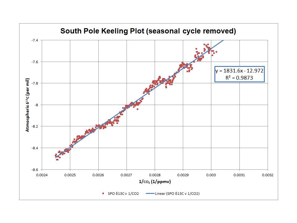
Here is a Keeling plot of the South Pole data (data source: Scripps CO2 program). The linearity reflects the constant value (on average) of the δ13C of the incremental CO2 and the value itself is given by the intercept of the line (-13.0‰, r2 0.99).
A second possible solution was given to me by Ferdinand: “it must be a coincidence”. This seems to me to be ‘rather unlikely’ given the near-identical results between the South Pole data and the Keeling plot for Law Dome (-13.1‰, r2 0.96), ref. Figure 1B in Kőhler et al (2006).
The third possible solution is the current (as far as I know) climate science model as published by Keeling et al (2017) which included the comment: “A further difficulty is that the global δ13C budget does not balance convincingly.” [Note: I downloaded this paper many years ago, but my links no longer work. This link appears to work: https://www.ncbi.nlm.nih.gov/pmc/articles/PMC5625891/ ] The authors highlight in the abstract that: “Using updated records, we show that no plausible combination of sources and sinks of CO2 from fossil fuel, land, and oceans can explain the observed 13C-Suess effect unless an increase has occurred in the 13C/12C isotopic discrimination of land photosynthesis.”
The problem in this case was that with the updated observations their ‘initial model’ did not match the observed rate of decline of atmospheric δ13C. After extensive analysis they found a possible solution was to introduce an increasing trend in one key parameter leading to a much-improved match of the model trend to observations. If you can access it from the reference given above, I strongly recommend reviewing the isotopic mass balance values as published in their Table S5. This is in the supplemental information to the paper.
However, I can show that simply assuming that the net δ13C of incremental atmospheric CO2 has remained at -13‰ since the start of their model (1765) actually fits their updated observations (both start point and trend) just fine, and hence provides a far better match than their initial model did. Interesting.
Or, to put it more succinctly … yes.
No, it does not. To learn what CO2 forcing means read my article..
https://greenhousedefect.com/unboxing-the-black-box
Ice core data suggests 800 to 900 years lag of CO2 increase after temperature increase, CO2 decrease following temperature decrease by some hundreds of years. Some of the criticism of this interrelation is various ideas about the difficulty of establishing either CO2 or temperature to that fine a distinction in time because of the things that happen to fallen snow and ice under pressure. This is for periods of thousands of years to 10s of thousands of years to totals of several hundred thousands of years. Some other paleo data has been reported as showing an even longer lag of CO2 change after temperature change.
With the data of this article might the difference in time between a CO2 measure and a temperature measure be much longer, perhaps a million or more years? If that possibility exists, then declaring leading or following might be an extremely biased conception.
AndyH, there is a very simple explanation for your correct observation. The estimated deep thermohaline return time is 800-900 years. So winter sea ice formation brine enhanced seawater with whatever CO2 sinks, and doesn’t get back to the surface to release its CO2 for that period of time. Covered in an essay (don’t remember which) in ebook Blowing Smoke.
Rud’s “Blowing Smoke” is a must-read.
Well that happens when people have no clue what they talk about.
First of all: which “extra energy”? The GHE is not about energy, or the “production” of energy, or the transfer of energy. The most important component of the GHE is the property of gases to heat adiabatically under pressure. Adiabatic means without heat transfer, or without energy addition if you will.
It is because of this specific property of gases that planetary atmospheres (or protostars btw.) become the hotter, the higher the pressure, the deeper within. It is also the reason why water can not generate a GHE btw., although it is way more transparent to SW than to LW radiation. Equally if an atmosphere was isothermic, you will still have plenty of “back radiation” towards the surface, but zero GHE.
Following the figures named above, consensus science would assume something like this..
13W/m2 of forcing equates to some 3.9K directly, or an elevation of about 600m in emission altitude. Then, in this instance, there would be very strong feedbacks increasing the temperature by a factor of 5. Equally the forcing would be enhanced to 65W/m2 and the emission level raised by about 3.000m in total.
At the surface the temperature would increase by almost 20K (=6.5 x 3), though a bit less once you consider negative lapse rate feedback. Because of this elevated temperature both at the surface and the very low troposphere, both now would exchange substially more radiation, like ~115W/m2. However, that is completely irrelevant, as it is a function of surface temperature, not the cause for it.
Thanks again Willis for “looking behind the curtain”.
I don’t think I’m alone in struggling to get my head around understanding all the permutations of push-pull factors in our “coupled, non-linear chaotic” climate system(s).
But speaking of ‘chaos’, it reminds of some points in my notes from a lecture series I attend – the current one being on “Chaos”.
• Scientists used to think that knowing the current state very, very accurately; we will almost always be close enough to predict a later state
• Chaos theory showed that even a very tiny uncertainty can grow exponentially fast to create completely different outcomes.
Many simple systems are quite predictable.
Complex systems are likely unpredictable.
Slight uncertainties in initial conditions
= Huge differences in long-term outcomes
Differences increase exponentially (non-linearly)
» Difference may increase 100-fold in 10X the time
I wrote perhaps the very first serious peer reviewed paper on the ‘business’ consequences of chaos theory. Had to do with explaining differential factory productivity.
Mathematically, a system is chaotic if it fulfills just two conditions :
Quality problems requiring factory rework fulfill both conditions. QED.
Thanks Rud.
This whole ‘chaos’ concept has now got me looking at everyday things and experiences through that particular prism.
A few sleepless nights ago, I re-watched that old classic movie “The Dam Busters”, and found myself trying to work out what of Sir Barnes Wallis’ considerations were ‘deterministic’, and what fell into the realm of ‘chaos’
Things that keep you awake at night, hey? 🙂
Do they even consider the question of whether instead, the climate controls CO2 levels? I mean clearly CO2 doesn’t control climate from around 15M years ago where CO2 spiked but the temperature barely moved. It could easily have been a million years or more. Right there is all the proof needed that CO2 isn’t the control knob.
Temperature DOES control CO2 levels via Henry’s law. That’s a simple explanation. What causes the temperature changes in the first place? Perhaps we’re still just missing something.
But I like Willis’ assessment of what this result means
There is simply no self doubt any more. The entire narrative is to find reason why CO2 is to blame and there is no reflection as to whether a result is valid.
Yes. And it does. Technically it works both ways. Temperature modulates CO2 levels and CO2 levels modulate temperature.
That only tells you that CO2 isn’t the only thing modulating temperature on those timescales which isn’t controversial at all.
Correct. Though Henry’s law is only part of the explanation.
There are a lot of things that modulate the temperature.
That only tells you that CO2 isn’t the only thing modulating temperature on those timescales which isn’t controversial at all.
The timescale could be millions of years. How is that not controversial? That’s what a control knob is, you turn it and there is a response. You can argue there is a lag but millions of years or even thousands of years isn’t a lag.
And once you acknowledge there are “other things” that can control the climate then you need to understand them before blaming CO2.
Maybe my wording was confusing. CO2 is a control knob. It’s just not the control knob. There are a lot of control knobs.
What evidence do you has that CO2 has any effect on temperature?
“have” rather than “has”, of course.
“CO2 is a control knob”
There is no evidence of that whatsoever.
But in GCMs, CO2 is the control knob. By design.
Aerosols, ENSO, dust, volcanic activity, tropical cyclone activity, biological activity, solar output, CFCs, HCFCs, CH4, NOx, ozone, contrails, stratospheric water vapor, ocean currents, land use changes, clouds, sea ice, etc. are examples of things that can modulate the atmospheric temperature in GCMs and other model types.
Lots more than that. Orbital, UHI, mountains, jet stream, tides, topography, uncertainty in measurements, and on and on.
Modulate is the wrong descriptor to be using. Temperature is not the signal being modulated. That is where too many climate scientists go off the rail. Temperature is only one component of a complex signal called climate. Think of it as more like a large orchestra where each instrument contributes rather than controlling. None are modulating others. This is where Fourier analysis originated.
Freeman Dyson said:
Notice the “tail”, the tail does not wag the dog.
Aerosols, yes. The rest, no in GCMs. GCMs running control runs don’t have climate change beyond about 17 years. They are literally designed to be climate change neutral.
They are in the GCMs that scientists look at plus a bunch of other stuff I didn’t mention because of the post length limit. I’m curious…do you know what a GCM is?
Anyway if I have at least convinced you that aerosols have a modulating influence then that should have been enough by itself to falsify your hypothesis that CO2 is the only modulating influence.
When they spin up, they do so to come to an equilibrium to iron out any inconsistencies in their startup values. That becomes a control run. Then they bumble along forever without creating climate change. At all. Its only when a forcing is added that anything changes.
So no, ENSO, cyclones, currents, ice cover, cloud cover changes, etc are NOT drivers and are NOT controlling features.
Aerosols are, yes but they’re tuned to best create historical correlations whilst remaining in justifiable/believable concentrations.
And do you actually believe anyone can project volcanic activity or even biological processes?
You don’t think ENSO has an effect on the atmospheric temperature?
You don’t think cyclones have an effect on the atmospheric temperature?
You don’t think ice cover has an effect on the atmospheric temperature?
You don’t think cloud cover has an effect on the atmospheric temperature?
Typical statistician response. Temperature is NOT CLIMATE. CO2 concentration IS NOT climate. There are causes and results. Climate science pointedly mixes these together. They see one thing with data, temperature, and determinedly focus on it since simple statistics allows sciencey conclusions.
I know they aren’t drivers in GCMs. They ONLY impact the temperature after the forcing. That’s why CO2 is the (only) control knob in models.
Yes aerosols too, but in their case they’re mainly used to reproduce historical changes.
If they impact the temperature in any way they are a driver, control knob, modulating influence, or whatever term you prefer. There are many factors (far too many to enumerate in a single post) that affect the atmospheric temperature and which GCMs capture. Don’t hear what I’m not saying. I’m not saying GCMs perfectly capture these factors. I’m not saying that GCMs capture all of them. The point I’m making is that CO2 isn’t the (as in singular) control knob. That’s just not how reality works.
You keep showing your lack of training in physical science.
To you temperature is the be all and end all of what climate is. IT IS NOT. It is your focus on radiative temperature that misleads you to forgetting that capital CLIMATE is the only important factor.
Climate encompasses many factors and radiation temperature is only one factor in climate.
Dyson had much to say about climate researchers using models to frighten people and reap consequent financial gain.
The folks at Oak Ridge lost out to the CO2 modeling folks for research money but it doesn’t mean their approach was wrong.
You keep mixing up results with drivers. Many of what you consider as drivers aren’t, they are results of temperature, not drivers of temperatures. As such the “results” are built into the CGM’s as factors that must be matched.
With a multiplicity of “drivers” it is beyond belief that they would all combine to generate a linear output from the CGM’s, i.e. the climate models. If some did and some didn’t generate linear outputs then there could be some argument about it. But they *ALL* generate nothing but linear outputs, only the slopes differ slightly.
Nope. That’s not what a control knob is, or does. Certainly not in this context.
Temperature is THE issue amongst warmists as they believe it is a good proxy for heat. It is why they use radiant flux since it has a direct effect based on temperature. When was the last time you saw a paper discussing enthalpy? They ignore the fact that dew point controls the minimum temperature which makes Tavg a joke.
Then you are using a different definition than everyone else. When I and others say “control knob” we are talking about an agent/actor that has a modifying or controlling influence on something. I often use the word modulate instead so as not to imply that a knob actually exists. I’m reminded of a time I used “control knob” once and someone actually thought I was implying there was a physical knob somewhere someone was turning.
So just know that if you disagree with me when I say something is a control knob or modulating influence I’m interpreting that as statement that you don’t think it “has a modifying or controlling influence”.
BTW…if you don’t think “control knob” is equivalent to “a modifying or controlling influence” then how are you defining “control knob”?
Irony
A control knob has an immediate and defined change in the property of what is being controlled. It is equivalent to a volume control setting the listening level via a deterministic functional relationship.
Think of turning a volume control and nothing happens until sometime later after another knob has been jockeyed with. That’s what CO2 does with climate.
bdgwx says
But the paper that brought the concept of the control knob Atmospheric CO2: Principal Control Knob Governing Earth’s Temperature has something to say about that. And its this:
That paper does not say that CO2 is the (as in singular) control knob. In fact, in no uncertain terms it contradicts your claim that no other control knob is considered. Citing a paper which says there are control knobs other than CO2 is not a great way of convincing me that CO2 is the (as in singular) control knob.
It kinda does though, doesn’t it. I gave the quote. CO2 is the one that controls the climate. That’s what they mean by control knob and that’s how the models work. Climate doesn’t change, they add the CO2 and it does.
Do aerosols impact climate? Yes. Are they the control knob? No.
Perhaps you’re sceptical of the AGW claim about CO2 being the control knob. I sure as hell am.
I think you’re overextending the interpretation there. I say that because the publication considers other control knobs with the title saying it is a “Principal Control Knob”. And if there is any linger doubt then surely figure 1 would put the nail in the coffin.
So if the CO2 control knob is turned up, temperature goes up. Somehow, this doesn’t seem to work very well, re, USCRN.
Lingering doubt? None at all. Its CO2 that they say controls the climate and that’s clearly reflected in Figure 1. That’s the control knob. The other things do not control the climate. They’re not control knobs.
Its not rocket science, its just that you want everything to be a control knob but in AGW parlance, they’re just not.
Does figure 1 not have an entry labeled “Other”?
It’s not about what I want. It’s an unequivocal and indisputable fact that there are many control knobs that effect atmospheric temperature. Just because CO2 may be the principal control knob on very long timescales in no way means it is the only control knob. And on short timescales it is not even the principle control knob.
The only thing here that’s indisputable is that you don’t understand what control means. Show me where a reputable someone has referred to another driver of climate in the other pile of Figure 1 as the control knob. Or even a control knob.
Your own citation does that.
Quote?
I looked for “knob”s in the paper and there are indeed a couple of references.
But not in control today. And
As a historical control.
So I’ll grant you that other influences have been considered as control knobs but they’re not in control of the climate today. CO2 is definitely the control knob in GCMs.
ENSO affects atmosphere temperature.
Cyclones are a RESULT of temperature, not a cause of temperature.
Ice cover is a RESULT of temperature, not a cause of temperature.
Cloud cover is a RESULT of temperature, not a cause of temperature.
You have your causality arrow backwards.
From AR4 (2007, WG-I report, Figure 10.36, page 828).
For some reason the IPCC didn’t provided results for such “overshoot” inputs to their climate model runs, on similar timescales at least, for either AR5 (2013) or AR6 (2021).
I’m not getting the relevance here which is unusual because all of your responses before have been spot on relevant. What am I missing?
Please provide a reference (or, even better, a link) to a peer-reviewed paper that includes a graph similar to AR4 Figure 10.36 for any “forcing” of the Earth’s climate system “driving” (at least) temperature and precipitation on decadal / century timescales, both up and down, other than CO2.
If you’re looking for proof that the IPCC considered factors other than CO2 then look no further than the FAR in 1990. I’m not sure why you need a graph to convince that CO2 is not the only considered, but assuming it is there are many of them in the FAR that can be reviewed. The SPM has several graphs of CH4, CFC11, CFC12, HCFC22, and NOx. The chapters discuss things other than GHGs including the Sun, aerosols, ENSO cycle, etc.
Going back to the historical works we see that Adhemar was the first to hypothesis that Earth’s orbit had a significant influence on the climate back in 1842. And, of course, Pouillet hypothesized that the Sun itself had a significant influence on the temperature of the atmosphere back in 1837. Both are early examples of scientists considering factors other than CO2 which are widely accepted as true today.
Make that 1827. And rereading his work I see he also considered geothermal energy as well though he felt that it was insignificant. Regardless we can add the geothermal to the list of non-CO2 factors considered before the turn of the 20th century and even before CO2 was considered.
You speak of modulation. Have you ever studied modulation? Modulation occurs to a carrier signal, either adding or subtracting depending on the phase and frequency.
To achieve the changes shown by Willis in the graphs on this thread, CO2 would have an extremely long frequency to achieve a modulation waveform whose frequency is shown in millions of years.
A control knob implies a direct effect on the value (normally an amplitude) of a signal. Climate science likes to show a direct correlation between temperature and CO2. What Willis is trying to show you is that there is no functional relationship where CO2 can directly increase or decrease temperature.
If you are going to use signal processing terms, use them as they are intended.
Does the reduction in CO2 cause the oceans to cool or does the cooling oceans cause the reduction in CO2.
Over the last 100,000 years or so, it’s always been the case that temperature changes precede change in CO2 levels.
The resolution of the longer data proxies is not sufficient to see whether the two changes were concurrent, as these “scientists” claim, or if the modern pattern continues into the past.
The data presented does not prove the claim that temperatures changes are perfectly matching CO2 changes.
“Does the reduction in CO2 cause the oceans to cool or does the cooling oceans cause the reduction in CO2.”
You put your finger on it, Mark. Rae, et al., pretty much assumed the direction of causality. More to come in comments.
There is a Youtuber calling himself Potholer56 who has come up with an ingeniously contrived way of explaining away this Inconvenient Fact.
I have a problem with this parts per million (ppm) thingy.
At 400 ppm, CO2 is 0.04% of the atmosphere.
At 4,000 ppm half a billion years ago, CO2 was 0.4% of the atmosphere.
Then there is nitrogen, at 780,000 parts per million. OMG!
Now here is the fundamental problem that I am sure is a concern of critical theory experts. CO2 plant food is 400 ppm. O2 animal food is 210,000 ppm. Can you spell injustice?
“How can an increase of 13 W/m2 in CO2forcing cause an increase of 115 W/m2 of upwelling surface longwave radiation?”
Obviously the magic of the GHE at its multiplicative finest.
Whatever happened to C02 being a lagging indicator of global heating? Am I that far behind the curve? Probably.
It is a lagging indicator – the method of paleo temp measurement in the article that Willis examined has been found to be unsuitable to the task by other researchers – please see the other comments way above for the link.
In the comments there is some confusion. The boron isotope and alekenone data are not used to estimate palaeotemperatures but palaeo-CO2 levels. The temperature estimates are largely based on the oxygen isotope record of benthic formaninifera. The oxygen isotope fractionation factor between carbonate and water varies by about -0.25 parts per thousand (-0.25 per mille) per degree rise in water temperature. This is the ‘temperature’ record shown in Javier Vinós plot.
It’s still there, and still ignored as an Inconvenient Fact by CAGW proponents.
Interesting article saying GW is caused by the sun not CO2. Hooray for our side!
https://www.theepochtimes.com/article/fixation-on-co2-ignores-real-driver-of-temperature-say-experts-5588495?utm_source=RTNews&src_src=RTNews&utm_campaign=rtbreaking-2024-02-24-1&src_cmp=rtbreaking-2024-02-24-1&utm_medium=email&est=AAAAAAAAAAAAAAAAceM4dwpahMPLzKoPtmpWRbd1xiQDb3kUvtLRGztEDsX37uQ%3D
It’s convenient that they had all those prehistoric mercury themometers so they know what global temperature was 60 million years ago.
The supposed relationship between CO2 and temperature for the past 60 million years is not such. They both decrease but do it at different times and rates. Particularly troublesome is the Oligocene, when a 10 million years warming trend started at a time when CO2 concentrations halved from 600 ppm to 300 ppm, constituting the bulk of the entire CO2 decrease for the Cenozoic.
I have used the data from a 2020 Science article with 22 authors:
Westerhold, T., et al., 2020. An astronomically dated record of Earth’s climate and its predictability over the last 66 million years. Science, 369(6509), pp.1383-1387.
This is their Figure 2D showing the CO2-temperature relationship:

I redid their figure for the past 52 million years using their data, shifting the axis and using the temperature data they provided instead 18O data. It shows the same but more clearly:

Their own data refutes what they conclude. Both CO2 and temperature are decreasing, but they do it at different times and rates. There is no correlation between them, and without correlation, there cannot be causation.
And both CO2 and temperature look like they are pretty much at a MINIMUM over the life of the planet !
The Holocene is in the bottom 10% of the Earth’s temperature range over time, with the Pleistocene being in the bottom 5% together with the Karoo ice age. About the same for CO2. The planet is incredibly cold and quite CO2-deprived even in 2023 (a record year), and this isn’t going to change significantly.
The future of this planet is the end of the interglacial in 1500-4500 years, followed by 70,000 years of glaciation. Humans are going to miss the ole times of global warming.
I have read on some Quora: At 400 ppm CO2 about 5% of the peak spectrum radiation is absorbed pr m. Average distance before absorption is 20 m. So within 100 meters longwave radiation will be thermalized, I think. And opposite with downwelling radiation. Most of the radiation will come from the 100 meters close to surface. With 2000 ppm this distance will be much smaller.
I think that this will make the numbers in Figure 8 physically impossible. It would mean a temperature gradient that show many degrees cooling from surface to the air above.
Easy. Air at 26 C holds twice as much VW as air at 15 C. One source says DWLW from current level of VW is around 75 W/m2.
The VW/Temp relation is exponential so the sensitivity will increase with temperature. Indicated in your fig.5.
WV (water vapor) of course, not VW
Air has the potential to hold more water vapor as it warms. However, that doesn’t mean that it will always be saturated with water vapor. To wit, a descending air mass will warm from compression. However, if there is no water available to supply additional water vapor, the relative humidity will decrease.
So what? It isn’t saturated today neither. The point is the different content then and now and the corresponding W/m2, which is probably less than 75 but impossible to know exactly.