by Javier Vinós & Andy May
“The complicated pattern of sun-weather relationships undoubtedly needs much further clarification, but progress in this field will be hindered if the view prevails that such relationships should not be taken seriously simply because the mechanisms involved in explaining them are not yet identified.”
Joe W. King (1975)
For those that prefer it, Christian Freuer has translated this post into German here.
2.1 Introduction
As shown in Part I of this series, the early 1980s saw a reversal in the consensus about an important sun-weather effect and studying the topic was discouraged. The adversarial academic environment resulted in very few scientists dedicating their research efforts to this subject. Despite the difficulties, important advances have been made regarding the sun-climate effect. Lack of interest and disregard for a competing climate change mechanism hypothesis by mainstream climatologists has resulted in these advances being ignored. They remain under-cited and unknown to most supporters and skeptics of the CO2 hypothesis. More importantly, they are not discussed in most climate papers, they are simply ignored.
These advances refer to climate phenomena that typically are not properly included in climate models due to lack of knowledge of how they happen or what causes them. They are not, or only weakly, reproduced by models, yet in most cases they can be detected in climate reanalyses where the models are constrained by a huge number of real observations.
Importantly, no hypothesis for a sun-climate effect can be correct if it cannot explain or accommodate the relationship between these phenomena and solar variability. The sun-climate relationship, at present, represents a black hole in modern climatology that keeps growing without anybody seeing inside it.
2.2 Effects on temperature and paleoclimatology
Paleoclimatology is the only subfield in climatology where a belief in an important sun-climate effect is considered. This is because the data obtained from proxy climate records of the Holocene often display a clear association with solar activity data obtained from proxy solar records. When one of us (JV) researched the climatic effects of the 2500-yr sun-climate cycle discovered by Roger Bray in 1968 (Fig. 2.1), he quickly found 28 articles studying proxies that clearly displayed this cycle (Vinós 2022). Of those, 16 (57%) explicitly state that changes in solar activity are likely the cause of the observed climatic changes, and only one explicitly rules the solar connection out. We are talking about profound global climatic changes of the distant past, similar in magnitude to the Little Ice Age (LIA) or modern global warming. Most paleoclimate researchers studying them conclude they were caused by changes in solar activity. Modern climatology cannot explain them since they took place at times when greenhouse gas radiative forcing changed very little.

In Fig. 2.1 the major Holocene subdivisions are labeled. The stratigraphic subdivisions are on top. The biological subdivisions are immediately below, showing a c. 2500-yr spacing (after Ammann & Fyfe 2014). Classical subdivisions based on temperature are across the bottom. The black curve labeled (a) is a global temperature reconstruction from 73 proxies (after Marcott et al. 2013; using original proxy dates and differencing average), expressed as distance to the average in standard deviations (Z-score). The black curve and the labels show the major climate changes during the Holocene. The blue/purple curve labeled (b) is the IntCal13 radiocarbon calibration curve used to convert radiocarbon dates (vertical, axis not shown) into calendar dates (horizontal). The blue/purple curve shows the major solar changes during the Holocene, they are after Reimer et al. (2013). The curve deviates from linearity during solar grand minima.
The Spörer, Homeric, Sumerian and Boreal 1 grand minima (blue ovals) are separated by multiples of c. 2500-yr, marking the lows of the Bray solar cycle B-1 to B-5, except B-4. These lows have been identified in radiocarbon data back to B-9 at 20,500 BP (Vinós 2022). Human population data is shown by (c), the red thick curve, a summed probability distribution of anthropogenic radiocarbon dates from Britain and Ireland as a proxy for human population. The red thin curve is a fitted logistic model of population growth and plateau, after Bevan et al. (2017). Significant downside population deviations generally match the lows of the 2500-year Bray cycle of solar activity (wide vertical blue bars labeled B-1 to B-5). The vertical pink bars are the 8.2 and 4.2 kyr abrupt climatic events (ACE).
The 2500-yr sun-climate Bray cycle constitutes a good example of the effects of solar variability on paleoclimatology, as it produces the most dramatic climate cycle observed in the Holocene. In terms of solar activity, it is defined by a sequence of Spörer-type grand solar minima that last 200 years and display a 20‰ increase in radiocarbon, spaced at 2500 ± 200 years with only a gap at c. 7,700 BP in the last eight periods since 20,500 BP (Fig. 2.1b; Vinós 2022). In terms of climate all the lows of the cycle are marked by periods of severe climate deterioration lasting over a century and reflected in multiple proxies, of which the LIA constitutes the most recent and the coldest example during the Holocene (Fig. 2.1a). In terms of the effects on human societies of the past, the Bray cycle lows are marked by periods of upheaval, population decrease (Fig. 2.1c), and civilization collapse, followed by societal advance afterward in response to a difficult situation.
The correspondence between past solar activity and past climate at the centennial and millennial timescales has caused authors like Rohling to say:
“In view of these findings, we call for an in-depth multi-disciplinary assessment of the potential for solar modulation of climate on centennial scales.”
Rohling et al. (2002)
Magny et al. write:
“On a centennial scale, the successive climatic events which punctuated the entire Holocene in the central Mediterranean coincided with cooling events associated with deglacial outbursts in the North Atlantic area and decreases in solar activity during the interval 11700–7000 cal BP, and to a possible combination of NAO-type circulation and solar forcing since ca. 7000 cal BP onwards.”
Magny et al. (2013)
Hu et al. express:
“Our results imply that small variations in solar irradiance induced pronounced cyclic changes in northern high-latitude environments. They also provide evidence that centennial-scale shifts in the Holocene climate were similar between the subpolar regions of the North Atlantic and North Pacific, possibly because of Sun-ocean-climate linkages.”
Hu et al. (2003)
Those three articles, between them, have 50 co-authors, among them some of the most respected in paleoclimatology. Either the current understanding of the sun-climate effect or the current understanding of paleoclimatology is wrong, as they are incompatible. In science when in doubt go with the evidence. Paleoclimatology has the evidence, while the current consensus on the drivers of climate change is based on computer models that reflect programmers’ ignorance and biases.
The increase in solar irradiance during the 11-yr cycle is about 1.1 W/m2. The expected surface warming for such a change in energy is only 0.025 °C and therefore below detection (Wigley & Raper 1990). Temperature data and reanalysis consistently show that the solar signal in global temperature is c. 0.1 °C, four times larger than expected from the energy change alone (Lean 2017) thus the need to find amplifying mechanisms. A very small energy increase from the sun is expected to result in a very small evenly distributed temperature change at the surface. This is not what is observed. The change in surface temperature manifests itself in an unexplained, but significant, regional and hemispheric variation and some regions cool when more energy is coming from the sun (Fig. 2.2). These differences can only be attributed to significant dynamic changes in the atmosphere and oceans when the solar output varies by only 0.1%.

Fig 2.2, (a), is a surface temperature change map during the 11-year solar cycle on a 5×5° grid from the 1996 solar minimum to the 2002 solar maximum using multiple regression. A pattern of discontinuous Southern Hemisphere mid-latitude warming is indicated by circles. The main western boundary currents in the Northern Hemisphere are shown by black arrows. Examples of long-term climate change responses to increasing solar activity obtained from paleo evidence or long climate records are labeled at their locations. Zonally averaged change in surface (b, black line) and 20 km height (b, red line) temperature, without a cosine area adjustment for latitude, after Lean 2017.
While the global average surface temperature increase with the solar cycle is only 0.1 °C, at 60°N it reaches 0.4 °C (above 1 °C at some areas). This general pattern of increased surface warming in the Northern Hemisphere extra-tropics and reduced warming in the tropics and Southern Hemisphere produced by increasing solar activity is not unlike the observed surface warming over the past 50 years. The surface temperature effect over North America confirms Currie’s (1993) finding that the solar effect on temperatures is opposite on both sides of the Rocky Mountains (see Part I). Another feature of solar induced warming is a pattern of alternating Southern Hemisphere (SH) mid-latitude warming and minimal change or cooling with a spacing of c. 7000 km (Fig. 2.2a circles). They are a tropospheric-ocean phenomenon and are more conspicuous at 5 km altitude (see Lean 2017) and probably reflect the global wavenumber-4 atmospheric wave whose importance for SH climate has been recently observed (Chiswell 2021).
This solar modulated atmospheric wave-train phenomenon could be related to the baroclinic annular mode (Thompson & Barnes 2014). As the atmosphere is intrinsically unstable, large-scale periodic atmospheric variability is very rare outside the tropics, as most atmospheric phenomena display red noise characteristics. One of the few examples is the baroclinic annular mode, a 25–30-day oscillation in the SH extratropical eddy kinetic energy associated with variations in the amplitude of vertically propagating waves, that has important effects on regional climate. The strong periodicity in the baroclinic annular mode, that coincides with the solar rotation period, together with the wavenumber-4 pattern over the 11-yr solar cycle, are suggestive of the baroclinic annular mode being modulated by changes in solar activity.
Lon Hood demonstrated that solar UV peaks modulate the Madden–Julian Oscillation. Daily changes in Madden–Julian Oscillation amplitude are modulated by UV changes, as the amplitude increases following UV minima. This amplitude modulating effect is greater during the winter and spring and is strongest during the easterly phase of the Quasi-Biennial Oscillation (Hood 2018). Given that the solar rotation period is close to one month, in the four solar cycles for which there is satellite data there are c. 500 solar rotations, allowing a much better statistical evaluation of this short-term solar effect on climate.
Another feature of the surface temperature pattern associated with the solar cycle is the warming displayed at the extra-tropical western boundary currents, particularly in the NH (Fig. 2.2a, black arrows). These are the preferred sites for transferring energy from the ocean to the atmosphere (Yu & Weller 2007). The incoming energy difference associated with the solar cycle is very small, but the change in ocean-atmospheric energy flux at those sites suggests that oceanic-atmospheric dynamic processes are regulated by changes in the solar cycle. Finally, the surface temperature pattern is essentially the reverse of the near-tropopause (20 km; Fig. 2.2b) pattern, except at NH high latitudes. Surface temperature changes are not the result of direct changes in TSI, since they are regionally very diverse and four times higher than the TSI energy budget allows. This suggests that the contrasting surface and tropopause zonal temperature patterns arise from troposphere-stratosphere coupling.
Not only the surface, but also the upper ocean displays a puzzling quasi-decadal change in temperature of c. 0.1 °C. White et al. (2003) analyzed the global tropical diabatic heat storage budget and found that the anomalous heating of the upper layer of the ocean to the depth of the 22°C isotherm yielded a value of ± 0.9 W/m2, that is nearly an order of magnitude larger than the surface radiative forcing of ± 0.1 W/m2 associated with the solar cycle (solar radiative forcing is ΔTSI/4 x 0.7). Even more, the quasi-decadal temperature change in the upper ocean is phase-locked to the solar cycle, something that modern climatology cannot explain.
The near total lack of interest by modern climatologists in the sun-climate effect neglects the abundant evidence from paleoclimatology and recent climate variations that correlate with the solar-cycle. This reveals our poor knowledge of the solar effect on climate change. We are all born ignorant, but some scientists choose to remain so regarding the sun-climate question.
2.3 Effects on the polar vortex
As reviewed in Part I (Sect. 1.6), it has been known since 1980 that the QBO modulates the strength of the polar vortex (Holton & Tan 1980). Seven years later, Labitzke (1987) discovered that changes in solar activity affected this modulation. It was the first solid, indisputable and climatically relevant sun-climate effect found in a 180-year-old quest. It also explained why the quest had been so difficult, as the effect is non-linear (not proportional to the total irradiance difference) and indirect, depending on the direction (QBO phase) and strength of the equatorial stratospheric winds.
The North Pole stratospheric temperature that Labitzke measured reflects the state of the polar vortex. A strong polar vortex is surrounded by strong winds, keeping inside an area of low pressure, low geopotential height (height of a given pressure), and low temperature due to radiative cooling. Higher temperatures denote a weaker and/or displaced polar vortex. When the polar vortex becomes weaker and/or displaced during the winter (i.e., higher North Pole stratospheric temperature), warmer air enters the Arctic, pushing the colder air below towards lower latitudes. A warmer North Pole with a weaker polar vortex indicates more severe winters in mid-latitudes. A higher frequency of colder winters in northern mid-high latitudes was a feature of the LIA.
Labitzke’s data showed that stratospheric North Pole temperature correlation to solar forcing depends on QBO state. During easterly QBO years stratospheric polar temperature is lowest when solar activity is highest, and highest when solar activity is lowest. The opposite occurs during westerly QBO years (Fig. 2.3a). Since the lowest easterly-year and highest westerly-year temperatures are similar, the largest temperature differences for the two different QBO states take place during solar minimum years. The average winter North Pole stratospheric temperature difference between both QBO phases during solar minima is an astounding 20 °C (Fig. 2.3b). The winter climatic effect of low solar activity over ample regions of the North Hemisphere is clearly disproportionate to the total irradiance energy difference. A difference that becomes irrelevant over the North Pole during the boreal winter, when it is in constant darkness.

Fig. 2.3 shows the effect of solar activity on winter North Pole stratospheric temperature. In panel (a) the black curve and light grey area show the winter (DJF) 10.7 cm flux average and standard deviation between Dec. 1955 and Feb. 2013. It is a proxy for solar activity, adjusted to an 11-year solar cycle. The colored curves correspond to winter temperature at 30 hPa (stratosphere) over the North Pole calculated as the average of the three more central values among DJFM monthly average temperatures (outlier discarded) and plotted according to the position in the 11-year solar cycle. The dark-red thick curve is the temperature for winters when the QBO presented average DJF values lower than –5.8 ms–1 (negative values denote easterly wind) corresponding to QBOe (easterly). Dark-red thin curve is the quadratic regression. Light-blue thick curve is the temperature for winters when the QBO presented average DJF values higher than 1.1 ms–1 (positive values denote westerly wind) corresponding to QBOw (westerly). The light-blue thin curve is the quadratic regression.
Fig. 2.3 panel (b) is a scatter plot of 30 hPa winter North Pole temperature, determined as in (a) versus tropical 30 hPa winter wind speed, for years with very low solar activity, corresponding to years 9 to 11 in the solar cycle as defined in (a), and indicated in the graph. Dark-red-filled dots are QBOe/temperature values used for the same color curve in (a). Light-blue-filled dots are QBOw/temperature values used for the same color curve in (a). Black thin curve is the quadratic regression. Strong El Niño years are labeled. The open circles are periods of low to slightly negative (easterly) wind speed. Data on North Pole stratospheric temperature is from the Institute of Meteorology at the Freie Universität Berlin. Data on the 10.7 cm solar flux is from the Royal Observatory of Belgium STAFF viewer.
According to Peixoto and Oort’s (1992) important book Physics of Climate, the unusually high correlation between solar activity and sea-level pressure or surface temperature over extensive areas of the NH, when the QBO phase is considered, appear to explain an important fraction of the total interannual variability in the winter circulation. But solar activity is not the only factor affecting polar vortex strength, it also depends on the QBO through the Holton-Tan effect (see Part I, Sect. 1.6) and on El Niño/Southern Oscillation (ENSO). El Niño years destabilize the vortex, and tropical volcanic eruptions stabilize the vortex which produces a warmer northern mid-high latitude winter.
Since Peixoto and Oort (1992), modern climatology appears to have forgotten about the important solar effect on the polar vortex and winter circulation. Dennis Hartmann’s Global Physical Climatology (2nd ed. 2016) does not mention Labitzke or her finding of a solar effect on winter circulation, and even fails to mention the polar vortex (not in the subject index). Surprisingly, it is the same situation with the more specialized An Introduction to Dynamic Meteorology (5th ed. Holton & Hakim 2013). Let’s remember that James Holton (1982) reviewed the possible physical mechanisms of solar variability’s effect on climate via dynamic atmospheric coupling, so it isn’t as if he didn’t know about it. Modern climatology is deliberately ignoring known evidence of a sun-climate effect.
2.4 Effects on El Niño/Southern Oscillation
The solar effect on ENSO is also ignored by modern climatology. A recent review on ENSO complexity by 45 prominent ENSO experts (Timmermann et al. 2018) completely fails to mention any solar implication despite the abundant bibliography on the subject (Anderson 1990; Landscheidt 2000; White & Liu 2008; Wang et al. 2020; Leamon et al. 2021; Lin et al. 2021). Deser et al. (2010) analyze the power spectrum of the Niño-3.4 (5°N–5°S, 170–120°W) SST time series and only mention the 2.5–8 years range, completely ignoring the distinct 11-yr peak in the series (Fig. 2.4b).
One of the authors (JV) recently studied the association between increasing solar activity and La Niña conditions in the Niño-3.4 region Oceanic Niño Index (ONI). A Monte Carlo analysis showed that the La Niña occurrences, which took place during times of rising solar activity (from 35 to 80 % of the ascending phase of the solar cycle), between 1950–2018, have only a 0.7% probability of being due to chance, demonstrating that ENSO is modulated by solar activity (Vinós 2019; 2022). The recent La Niña conditions since 2020 after the December 2019 solar minimum can only have reduced the already low probability that the association is due to chance.
The solar-ENSO modulation is uncovered by a simple frequency analysis of ENSO modes. ENSO displays three temporal modes: El Niño (warm mode), La Niña (cool mode), and Neutral. The ENSO system is usually considered to be an oscillation between El Niño and La Niña modes due to their opposing temperatures. This view appears to be incorrect. NOAA’s Climate Prediction Center classifies ENSO winter modes (year corresponding to January) according to SST data in the Niño-3.4 region (Domeisen et al. 2019). Using this classification, it is trivial to demonstrate that La Niña years strongly anti-correlate to Neutral years, not El Niño years (Fig. 2.4a) for the 1960–2020 period (1962–2018 shown using a gaussian filter).

In Fig. 2.4, (a) is the frequency of Niña years (medium blue thick line) and Neutral years (light brown thick line) in a 5-year centered moving average (gaussian filtered) between 1962–2018 showing an almost perfect anti-correlation for the entire period. The small boxes along the bottom are the ENSO mode classification after Domeisen et al. 2019, with dark red boxes for Niño years, and colors matching the curves for Niña and Neutral years. Asterisks mark strong Niño and Niña events with ≥1 °C anomaly in Oceanic Niño Index. The fine grey line is the number of yearly sunspots.
Fig. 2.4 panel (b) is the power spectrum of the 1900–2008 Niño-3.4 SST anomaly time series after Deser et al. 2010. An arrow marks the 11-year frequency peak that might correspond to the solar cycle effect. Panel (c) is the Dec–Feb average warm water volume anomaly above the 20 °C isotherm between 5°N–5°S, 120°E–80°W. The data is from the TAO Project Office of NOAA/PMEL.
Los Niños typically take place every 2–3 years (range 1–4 years), so there are always 1–3 Niños in a 5-year period. La Niña and Neutral years are more variable, as there can be 0–4 of each in a 5-year period. The strong anti-correlation between La Niña and Neutral years indicates ENSO has been profoundly misunderstood and even its naming is incorrect, as it should be La Niña/Southern Oscillation. Analysis of the warm water volume in the equatorial Pacific (Fig. 2.4c) indicates that energy tends to accumulate during Niña years, and it is released during Niño years, with Neutral years somewhere in between. Energy tends to accumulate in the equatorial Pacific, one of the major solar energy entry points into the climate system. The ENSO system oscillates between accumulation (Niña years) and inefficient distribution (Neutral years). When the system accumulates excess energy, Los Niños occur to efficiently spread the excess through the rest of the climate system.
The La Niña/Neutral oscillation is phase locked to the solar cycle (Fig. 2.4a). El Niño frequency is also affected by the solar cycle, as other authors have noted (Landscheidt 2000), but not so strongly, and the occurrence of Niño years slightly perturbs the Niña/Neutral fit to the solar cycle. This solar effect on ENSO explains the 11-year frequency peak in the Niño-3.4 SST power spectrum. It also explains why multidecadal periods of high solar activity, like the modern solar maximum, tend to display less Niñas, and why the period of reduced solar activity since 1998 has displayed more frequent Niñas with less negative warm water volume anomaly values. Coinciding with the Pause in global warming, warm water volume anomalies have significantly fewer negative values, reaching less than one fourth of previous negative values (Fig. 2.4c). El Niño is the odd one out in the Niña/Neutral oscillation, which explains why El Niño comes in different flavors (Central Pacific versus Eastern Pacific) and displays an enormous variability during the Holocene (Moy et al. 2002), with Niño activity very reduced during the Holocene Climatic Optimum. El Niño flavor, frequency, and intensity respond to the requirements of the poleward meridional energy transport process.
One can only wonder that, if modern climatology wasn’t so blind to the sun-climate effect, the solar modulation of ENSO would be common knowledge and discussed in reviews like Timmermann et al. (2018) and Domeisen et al. (2019). It is embarrassing, and an indication that modern climatology has lost its way, that it has taken a molecular biologist to notice.
2.5 Effects on Earth rotation
Solar activity affects the Earth’s speed of rotation. The effect is small, but it has been measured since the advent of atomic clocks in the late 1950s. This solar effect has been noticed periodically by researchers, reported, ignored, and forgotten, only to be noticed again by another researcher believing it was an original discovery. The first report appears to be by René Danjon in 1962. In 1971 Rodney Challinor, with 14 years of data, related the annual changes in the length of day (LOD) to the sunspot cycle. He suggested that changes in the global atmospheric circulation induced by solar activity changes might be responsible for the effect on Earth’s rotation rate (Challinor 1971). Jan Vondrák (1977) and Robert Currie (1980) also rediscovered the solar-Earth rotation relationship. In the 1990s Daniel Gambis (Gambis & Bourget 1993) and in the 2000s Rodrigo Abarca del Río (Abarca del Río et al. 2003) continued the studies on the solar-Earth rotation relationship. More recently Le Mouël et al. (2010) and Barlyaeva et al. (2014) investigated possible mechanisms of this relationship.

In Fig 2.5 (a) the monthly ΔLOD for the 1962–2018 period is plotted. The inset shows two years of data with four semi–annual components corresponding to northern (NH) and Southern Hemisphere (SH) winters. The panel (b) black curve is the 3-point smoothed amplitude of the NH winter change in ΔLOD from weekly data after 31-day smoothing. Lower values indicate a larger change in Earth’s rotation speed. The red curve (right scale) is solar activity as determined by 10.7 cm flux (solar flux units, gaussian smoothed). The dotted curve (right scale) is a Fast Fourier Transform with a 4-year window of the time derivative 0.5-yr component of LOD, 30-month smoothed, after Barlyaeva et al. 2014.
It has been demonstrated that, for periods of time between 14 days and 4 years, changes in the atmospheric angular momentum (AAM) of the troposphere and stratosphere account for over 90% of the changes in LOD (Rosen & Salstein 1985), as the Earth’s rotation rate must adjust to keep the total momentum of the Earth system constant. Seasonal variation in ∆LOD has been known for decades to reflect changes in zonal circulation (Lambeck & Cazennave 1973). For a discussion of zonal winds, mostly from UCLA, see here. The biennial component of ∆LOD reflects changes in the QBO (Lambeck & Hopgood 1981), while the 3–4-year component matches the ENSO signal (Haas & Scherneck 2004). The 2015–16 El Niño produced a ∆LOD excursion reaching 0.81 ms in January 2016. A very close fit between the semi-annual component in ∆LOD and solar activity should not be expected given these other causal agents.
The link between changes in ΔLOD, changes in AAM, and solar variability is very straightforward, and necessarily must go in the direction “solar → atmosphere → rotation.” The momentum of the Earth system is conserved at the scales involved and it is not possible that changes in the speed of rotation of the Earth affect solar activity. A relationship between multidecadal changes in ΔLOD and changes in climate was proposed by Lambeck and Cazenave (1976). Without considering a solar implication, they reported on the similarity between the trends of numerous climate indices for the past two centuries and changes in ∆LOD. In particular, Lambeck and Cazenave noted that LOD variations correlate well with global temperature and ground pressure, both of which are indicators of global wind circulation. They concluded that periods of increasing zonal winds correlate with accelerating Earth rotation while periods of decreasing zonal circulation correlate with deceleration. They found a lag of 5–10 years in the climatic indices. Their result has been reproduced multiple times (e.g., Mazzarella 2013).

The AAM can be reconstructed back to 1870, and its decadal changes in the annual and semiannual components (related to the annual and semiannual components of ∆LOD) display a correlation with the 11-yr solar cycle. Interestingly the correlation between the annual component and the sunspot number underwent a phase shift c. 1920 (Fig. 2.6B). This is a time when multiple sun-climate correlations inverted (see Part I, Fig. 1.3), discrediting sun-climate correlation studies. We do not know what causes these inversions in the climate response to solar activity and probably we will not know until a new inversion takes place, since we need to know what happens in the stratosphere during them. They appear to occur every 80–120 years (Hoyt & Schatten 1997). However, we can conclude two important things from the existence of these sun-climate inversions. First, that solar activity affects climate through its effect on atmospheric circulation (AAM), not through differences in total irradiance. And second, when the solar effect on the annual component of the AAM shifts phases, the solar effect pattern on surface temperature and precipitation inverts. The simultaneous occurrence of the phase shift in AAM (Earth rotation) and the sun-climate pattern inversion at c. 1920 demonstrates that these shifts are an intrinsic feature of the sun-climate effect.
Since the solar effect on Earth’s rotation rate and global atmospheric circulation are deliberately ignored by modern climatology, they are not included in general circulation models. This allows the IPCC to wrongly conclude that solar variability has no significant effect on climate change since 1850. The reality, however, is that a great part of the climate change that has taken place during the 20th century has been due to the modern solar maximum.
2.6 Effects on planetary waves
In 1974, Colin Hines proposed that the sun-climate effect could be accomplished by modulating the planetary waves propagation properties of the atmosphere, and James Holton agreed that such mechanism was viable, but objected that little evidence existed for it at the time (Hines 1974; Holton 1982). This was not entirely correct. Geller and Alpert (1980) not only demonstrated the viability of the Hines mechanism but showed that changes in the sun’s ultraviolet (UV) emissions, by changing the stratospheric thermal structure, could be responsible for changes in the mean zonal wind, resulting in inter-annual variations in stationary planetary wave patterns that could induce very significant changes in regional climate. Their modeling results not only quantified the magnitude of the expected effects but indicated that the tropospheric planetary wave response to solar-induced changes in the zonal mean state of the stratosphere ought to be regional, very evident at some longitudes and latitudes, and absent in others (Fig. 2.2).
Waves in the atmosphere (Fig. 2.7) are oscillatory motions that result from a balance between the inertia of a parcel of air that has been set in motion and a restoring force. These oscillatory motions produce periodic changes in atmospheric variables (pressure, geopotential height, temperature, or wind velocity) that may remain stationary or propagate horizontally or vertically. Atmospheric waves transmit energy and momentum without material transport of air parcels to remote regions on time scales much shorter than the transit time for air parcels. The momentum and energy are fed into the background flow as the wave dissipates or breaks, altering it. Most weather disturbances are associated with one or more types of atmospheric wave (Holton 2003).

In Fig. 2.7, (a) is a photo of atmospheric waves made visible by Saharan dust off the northwestern coast of Africa. The photo is from NASA. Photo (b) are of atmospheric waves caused by the Tonga 2022 eruption that circled the globe. The photo was captured by NOAA’s GOES-West satellite IR channel. Tonga is located at the bottom left of the image. From Mathew Barlow and after Duncombe (2022).
Vertically propagating planetary (Rossby-Haurwitz) waves are generated by flow over continental-scale topography, by continent–ocean heating contrasts, and by nonlinear interactions among transient tropospheric wave disturbances. Their restoring force is the potential vorticity latitudinal gradient induced by the Coriolis parameter due to planetary rotation. Planetary waves zonal wavenumber is an integer designating the number of waves around a latitude circle, thus at 60° a wavenumber 1 planetary wave has c. 12,000 km meridional scale. The vertical propagation of stationary planetary waves requires the presence of mean westerly winds of speed lower than a critical value, in what is known as the Charney–Drazin criterion. In practice, zonal wavenumbers 1–3 account for over 96% of wave propagation into the extratropical stratosphere, and this happens only in the winter hemisphere.
Small changes in solar UV energy can cause big changes in the energy and momentum delivered by planetary waves to the stratosphere. These are then reflected in changes in the troposphere, through stratosphere-troposphere coupling, as suggested by Hines (1974), and shown by Geller and Alpert (1980). This process constitutes the basis of the “top-down” mechanism of sun-climate effect. This process or mechanism bypasses the problem of the small change in solar energy output during the solar cycle, as the energy to affect climate is provided by planetary waves, which alter the global atmospheric circulation in regionally diverse patterns. Kodera and Kuroda (2002) showed that with the arrival of winter, the stratospheric circulation changes from a radiatively controlled state to a dynamically controlled state, and the transition is modulated by solar activity, with the solar maximum prolonging the radiatively controlled state. This modulation affects the strength of the stratospheric sub-tropical and polar night jets, and the Brewer–Dobson circulation.

Perlwitz and Harnik (2003) provided evidence that planetary waves reflected in the stratosphere on certain winters had a tropospheric effect. Nathan et al. (2011) showed that the zonally asymmetric ozone field was very important in mediating the effects of solar variability on the wave-driven circulation in the stratosphere. The study of planetary waves in the stratosphere is recent and difficult to carry out. Powell and Xu (2011), using two reanalysis datasets and satellite microwave sounding unit observations, constructed a planetary wave amplitude index for the 55–75°N stratosphere and showed it was associated with the Arctic Oscillation. They found substantial shifts in the stratospheric state due to changes in wave amplitude and pattern anomalies. The main ones were associated with a 2-year oscillation that was in phase with the solar cycle. During solar maxima planetary wave amplitude was reduced, while during solar minima changes in the meridional temperature gradient and vertical wind shear lead to an increase in planetary wave amplitude (Fig. 2.8). The detected solar cycle effect may account for 25% of the variability in wave amplitude (Powell & Xu 2011).
The Powell and Xu (2011) finding provides direct observational evidence for the Geller and Alpert (1980) study. In their study, Geller and Alpert showed that a 20% change in the mean zonal flow at 35 km height or lower would be the required order of magnitude to produce the observed interannual variability in the tropospheric wave pattern at middle and high latitudes. The finding by Powell and Xu that the solar effect might explain 25% of stratospheric wave amplitude indicates that the UV solar effect, coupled with ozone variability, can explain the important sun-climate effect on winter atmospheric circulation first detected by Labitzke and van Loon (1988).
2.7 Conclusion
This part (2nd of the series) demonstrates the existence of a wealth of knowledge about the sun-climate effect, laboriously produced by scientists who have not received proper credit for shining light on what is probably the most complex, most controversial problem in climatology. This knowledge provides sufficient clues about the sun-climate effect mechanism.
It is no longer acceptable to say that solar variability in total irradiance is too small to have a significant effect on climate, when there is so much evidence that variations in total irradiance are not how solar variability mainly affects climate.
It is no longer acceptable to say that indirect effects of solar variability are too uncertain since their mechanism is unknown when clear evidence for the mechanism is published and ignored.
It is no longer acceptable to only consider changes in total irradiance in model studies and then declare that the modern solar maximum did not contribute to modern global warming.
It is no longer acceptable to reject a sun-climate effect based on the lack of a simple correspondence between surface temperature and solar activity, when evidence suggests that the solar effect on climate works through changes in atmospheric circulation.
If it remains acceptable, then we are building the foundations of climate change science on a false premise that prevents us from understanding it. It will set back the scientific advancement of climatology by decades, just as the refusal to accept the evidence for continental drift set geology back four decades. And it will have huge repercussions for the reputation of science, as most climatologists provide a justification for expensive socioeconomic policies while ignoring an important, well-documented, solar-climate connection.
The bibliography can be downloaded here.
A list of abbreviations used can be downloaded here.
This post was first published on Climate Etc.
Tremendous piece of work. But the warming of the past 40 years was not due to the sun.
I explain it here.
https://breadonthewater.co.za/2022/03/08/who-or-what-turned-up-the-heat/
Global maxima are falling from ca. 1996 or 1997.
Obviously it was also not due to more CO2….That is just crazy nonsense.
Regarding your investigation of waste water impacts on ocean release of CO2. While it is certainly true that cumulative plant emissions have significant local impacts, in aggregate, when compared to the bulk of the ocean water they are a drop in a bucket.
Nothing is linear when it comes to climate. But you can only explain the heating during the instrumental record by studying the adjustments done to them.
Nonsense. Temperature gradients are linear as is easily seen by looking at the divisions on a thermometer.
My, my, I don’t think you understand what Robert is saying.
Good to see some serious science is being done in addition to all the ridiculous climate change fear mongering.
More importantly, they are not discussed in most climate papers, they are simply ignored.
standard practice for major problems
minor problems are explained or adjusted away
major problems are waved or eye-rolled away
“The increase in solar irradiance during the 11-yr cycle is about 1.1 W/m2. The expected surface warming for such a change in energy is only 0.025 °C and therefore below detection (Wigley & Raper 1990)”
First, why use a 30y old estimate made before the TSI industry matured?
Second, it’s wrong. Recent solar cycles net changed SST anywhere from 0.1°C – 0.3°C:
http://climate4you.com/images/SunspotsMonthlySIDC%20and%20HadSST3%20GlobalMonthlyTempSince1960%20WithSunspotPeriodNumber.gif
Solar cycle #24 TSI was responsible for a ~0.35°C annual rise from 2008 to 2016 [~0.6°C monthly] the ~1 yr lags shown with annual data are really on the order of months:
HadSST3 during SC24 exhibited growth with rising TSI and particularly after 2013 when annual TSI exceeded my decadal sun-ocean warming threshold. Then it declined with declining TSI, predictably.
Now we await a SST increase from SC #25, as I predicted back in 2018 in my AGU poster. During this solar cycle, temperatures will likely increase to and exceed the 1.5°C ‘limit’, as I expressed here in a comment several months ago.
I defined the solar modern maximum back in 2014 as being from 1935-2004, when sunspot activity averaged 108.5 SN. Javier knows about the 70y Mod Max, which is why he repeats it, but he denies it’s true power over the ocean.
Climate changed due to sunspot activity higher than 95 SN, the sun-ocean warming threshold I also determined back in 2014. Nothing has changed. The climate is driven by TSI, not by the tail wagging the dog, ie, atmospheric changes.
There is a 2-month lag between the UAH troposphere temperature and HadSST3 global, so the atmosphere doesn’t drive the ocean. Since the ocean clearly drives the troposphere, there’s no point in pretending the even higher atmosphere controls the ocean at all.
I was going to wait to read more parts before commenting. But part two points to something I personally experienced before (consulting to a heavy truck assembly plant). Even built a computer model of it and ran a sales experiment to prove it.
Climate is a nonlinear dynamic system. Precise definitions. Nonlinear means there are feedbacks. Dynamic means feedbacks are not instantaneous. Both statements are trivially obvious about weather and hence climate (envelope of at least 30 years of weather).
ALL nonlinear dynamic systems are mathematically chaotic. Sensitive dependence on initial conditions is only one of many hallmarks of mathematical chaos. Strange attractors in N-1 Poincare space is another. Many books delve into this, from the layman’s CHAOS to serious math treatises.
One hallmark of chaotic systems is ‘amplification’, commonly known as ‘the butterfly effect’. That is, a very small change of state (butterfly flapping its wings) can result in very big differences down the line (a hurricane). That is what we found with heavy trucks needing rework (parts missing or wrong at the end of the assembly line, parked awaiting rework before delivery).. A small shift from 39% custom orders to 41% custom orders caused the expensive rework backlog to more than double within two months. Wrote it up as part of a peer reviewed paper about 1991.
What Javier and Andy discuss in part two here is something very similar, and they are positing ‘butterfly effect’ mechanisms no different in principle than the ‘magical’ 40% custom truck orders threshold we proved both via math models (using the systems dynamics visualization language STELLA), and experimental observation.
So please pay close attention. Judith hosting this is serious stuff.
Run,
you seem to have completely mis-understood the post. The amplification mechanism they describe must be linear and has nothing to do with the butterfly effect. If Javier and Andy want to claim that they and others have detected a clear signal from the sun in the climate record then the response has to be linear since all they are doing is looking at aligning different periodic cycles. Fig 2.6 is a clear example of solar cycles aligned to climate cycles. In a nonlinear system the output frequencies will be different from the input ones and so this simple approach would not work.
Secondly if the amplification was the same as the butterfly effect then it could never be seen since it would be different every time (sensitive dependence on initial conditions). Hence if your claim was true sometimes solar variations would lead to increases in temperatures and other times they would lead to decreases in temperatures. And there would be no way to distinguish that from noise in the historical data.
Nope. Nothing they say implies linearity, which implicitly means monotonic changes. Their charts are not generally monotonic.They are exponential amplifications except in certain amplification/deamplification midrange portions.
Rud,
linearity does not imply monotonic changes. If the input to a linear system is changing periodically then the output will change periodically as well. A linear system will have the same frequency content at the output as the input signal while a nonlinear system can have different frequency contents. Javier and Andy are looking for periodic signals in the climate record that match the periodic output of the sun and so implicitly they are assuming that the climate is a linear system.
You are totally out in left field. Frequency changes due to a non-linear system just don’t compute. A non-linear system can result in harmonics of the fundamental being generated but almost impossible for the harmonics to be larger than the fundamental without filtering and amplification. Again, see Fourier.
If what you say it true, Fourier analysis of a complex signal would never reveal the fundamental frequencies in any non-linear system. You could kiss off any circuit using non-linear devices like inductors or capacitors. Non-linear doesn’t mean changing frequencies, it can also and most probably does, result in a complex amplitude changes. Variance in frequencies will result in phase changes that result in various amplitudes. This may look non-linear but is fully analyzable.
Jim,
A nonlinear system can become unstable through a Hopf bifurcation and start to oscillate the moment it is driven past some threshold. At which point it oscillates with its own characteristic frequency than is independent of any driving frequency. It can also further undergo a period doubling if driven harder meaning that the frequency will change again. So there is no obvious relationship between the input and output frequencies.
I think this covers your criticism.
Again, if true, the earth’s climate system that responds in this fashion will probably never be analyzable due to the number of factors at play. it could only be displayed in a probability space which would preclude any predictions being deterministic. That may be what is at work. But, CO2 would certainly be a small piece of the puzzle.
I’m not mad at you Rud, I just want you to think about this a little.
“So please pay close attention. Judith hosting this is serious stuff.”
Would you say the same exact thing someday about my or someone else’s work if she hosts my sun-climate discussion, or someone else’s?
Haven’t you realized Javier’s entire preposition is based on first putting TSI down?
His method is no different than inverted IPCC climate science propaganda. Enough said.
The reality is I have already solved the sun-climate problem with TSI, years ago, and not with butterfly nor secondary or tertiary solar effects, so Javier’s promotional book blitz is going to end up being largely in vain as something that might move the climate consensus.
“A small shift from 39% custom orders to 41% custom orders caused the expensive rework backlog to more than double within two months.”
You just unwittingly described threshold and accumulation theory, which is how TSI works on the ocean [climate]. 40% custom orders was your threshold above which your rework accumulated significantly. Perfectly analogous to how TSI above the threshold warms the ocean, above which the ocean accumulates heat. Exact. same. principle.
Tell you what, BW. Explain your theory as clearly as Javier has (I am not saying I agree, only that his is not implausible.)
After only 2 of 5 of his posts, do you already clearly know what his theory is?
Javier’s exact theory is so far unclear. Further I’m not sure it’s a very original idea, as WUWT commenter ren has already posted here and elsewhere many times over many years about the winter polar vortex effect re stratospheric intrusions, and with respect to the solar cycle, so how do Javier’s ideas differ from ren‘s posts or others in the literature with possibly similar themes?
We are just setting the background for what needs to be known to fully understand the hypothesis in four posts. However, enough information has already been given so sharp people can see where the solar effect on climate resides. Fifth part will discuss the hypothesis and sixth part will discuss what is really the climate change “control knob.”
As I said, in a comment at Judith’s place, there are several hypotheses for a solar effect on climate. Without being exhaustive, the “top-down”, the “bottom-up”, David Evans’ “Notch delay”, Stephen Wilde’s based on ozone, Bob Weber’s based on TSI, some Finnish researchers on particles, Ulric Lyons on solar wind, and Svenmark’s cosmic ray effect on clouds. Obviously they cannot all be correct, even if they all contribute to the effect, as they all claim to be the main one. Only the first two have significant support in the scientific bibliography.
My hypothesis has been built on top of the “top down” hypothesis, completely incorporating it, but has a different explanation for the climate effect, supported by evidence. So it is much more ample and focuses on the so far ignored effect on the most important climate variable. Since the “top down” hypothesis is the best supported hypothesis by data, models, and reanalysis, I start from an advantageous position.
My perspective is top down, how the Sun drives heat and cold waves, or rather Northern Annular Mode anomalies. It’s hard to imagine anything other than the solar wind variability doing that. The solar wind explains the AMO very neatly too, it is colder when the solar wind is stronger, like the mid 1970’s, mid 1980’s, and early 1990’s:
“Obviously they cannot all be correct, even if they all contribute to the effect, as they all claim to be the main one.”
Alarmists buzz each other up with their baloney, like team work, and maybe collective narcissism. While sceptics often bicker, suffer from not invented here syndrome, and resist accepting anything which makes their hypothesis redundant, the irrefutable hero syndrome. When what we really need is team work.
“ALL nonlinear dynamic systems are mathematically chaotic”
Northern Annular Mode anomalies are driven at daily to weekly scales by changes in the solar wind. That is not chaotic.
I wish I could get some of my “settled science” friends to spend some time here. That last discussion on Putting it into reverse article really showed what a high caliper group we have here. This article may not be quite as much “fun” but we’ll see. I’m out gunned here, I am more just a WUWT groupie.
How about adding skepticism to your arsenal.
So Mr. Oliver is not certain that the science is settled, and you suggest he should add some skepticism?
I think your Trollbot 5000 comment generator may be broken.
Funny how the guy who wants others to be skeptical, refuses to ever question the claims of his masters.
Some people give good advice but don’t follow it themselves.
A common human failing.
Perhaps follow some of your own advice?
Look at the mirror.
This “high caliper [sic] group” have brains like a vice grip ! 🙂
Appropriate for examples using truck manufacture until someone puts the brakes on,
Calibre, not all of us have leg braces..
It is not correct to say that evidence for sun/weather/climate effects are deliberately ignored for non-scientific reasons. They are ignored as they should be because the evidence is too weak and most of the claims [including the ones trotted out in the post] are too poorly documented or presented [e.g. no error bars or poor statistics]..Once the evidence becomes good, scientists very rapidly accepts the effects [e.g. that stones can fall from the sky or that continents move around, but until then, it is good science to be skeptical. As Sagan reminded us: “extraordinary claims require extraordinary evidence”. And such is simply not there.
Leif, you may be right and Javier wrong. I am not and never will be a solar expert to sort that out. All I said was, the ‘butterfly effect’ mechanisms they posit cannot be ruled out by first principle mathematics of chaos theory. I gave a supporting general proof. Are these post posits real,dunno.
Leif, don’t you think the people promoting CO2 theory have made many many extraordinary claims without providing extraordinary evidence? No matter how you slice it they have very assiduously ignored the fact that CO2 lags SST.
The problem is CO2 theory was entrenched politically at a time when TSI was in it’s infancy, and decisions were made without the benefit of our better modern data, both solar and climate.
The evidence I have provided for simple TSI forcing, albeit without error bars but with decent statistics, is better than what the CO2 side offers, better than convoluted atmospheric theories.
What is the current global average temperature with error bars? What was it 100 years ago, 500, 1000, 2000, 3000, 6000, years ago, etc. with error bars?
There’s really not much to see here.
Leif,
There is plenty of evidence presented in this post. I notice you do not try and refute any of it. Why? Your comment falls flat due to lack of specifics. Arm waving is not evidence. Give us extraordinary evidence we are wrong. We only claim that solar variability has a role in climate change, as all the palaeoclimatological evidence tells us, how is that wrong? Be specific.
We also present evidence that solar activity and the QBO affect the polar vortex, winter circulation, temperature, and SLP in the NH high latitudes. What contrary evidence do you have?
What about the correlation between ENSO and the Sun? What contrary evidence do you have?
Finally, what about the evidence we present relating solar activity and the length of day?
“Give us extraordinary evidence we are wrong”
The shoe is on the other foot.
Clearly all you present has not managed to convince the majority of scientists.
If the evidence were good, acceptance comes easily. But it is not good and does not convince. You say so yourself as you bemoan that your ‘evidence’ has not led to general use of the claimed relationships.
Willis has in these pages debunked many of the claimed effects. No need to repeat that effort, as nothing can get true believers to see the errors of their ways.
Now, personally, I would love you to be correct as that would do wonders for funding of solar science, but, alas, I don’t see that coming any time soon.
Leif, I must note that you are inflating Willis’s excellent contributions. What he has done (quite well) is to disprove the notion that there is a <i>simple</i> and <i>direct</i> relationship between solar variability and terrestrial climate changes.
This hypothesis by Javier and Andy is not positing any such relationship – and is therefore not “debunked” by anything that Willis has posted.
Leif, I believe this is true of you – and probably the colleagues you work with. You are a fortunate man.
But there are far too many for which the rallying cry is “profitable claims require fraudulent evidence.”
The “Greenhouse Gas Hypothesis” for climate has been quite thoroughly disproven. Not just weak evidence – false evidence. Not just poor statistics – deliberately manipulated statistics.
Javier and Andy may, or may not, manage to make a convincing case for their “Solar Variability Hypothesis” – but at least I can be confident that they will not present lies as truth.
“Once the evidence becomes good, scientists very rapidly accepts the effects”
Pull the other one, history is littered full of pompous authority figures who resisted the emergence of new findings for decades. Given the money invested in the green agenda, the last thing they want to know right now is about how the Sun discretely drives all the big heatwaves they say will be happening every other year by 2050 because of CO2.
“It is no longer acceptable to say that solar variability in total irradiance is too small to have a significant effect on climate…”
Well if you’re talking about a few decades, yes it is. This whole article is attempting to confuse the reader, talking about Holocene scale Milankovitch cycles and centuries long sunspot cycles and a few other red herrings, which are far too weak to have any but the smallest effect over decadal time frames. Anything, anything, but CO2, eh?
Meantime the elephant in the room keeps expanding and the denial factory keeps chugging along. Shame.
Straw man alert: “an intentionally misrepresented proposition that is set up because it is easier to defeat than an opponent’s real argument” (Oxford).
You’re going way over his head. He can’t even follow simple grammatical rules.
The elephant in your room. Loydo, is the following:
Loydo provided a criticism of this article. You ignored that criticism and responded with a character attack unrelated to the original comment
Loydo made a character attack – which Rud replied to with factual information. Here is a character attack – you are completely ignorant of what ad hominem means.
Loydo criticized the article
Istvan responded with a generic character attack: Essentially saying many climate alarmist predictions have been wrong in the past, so who cares what you think.
Now both you and Istvan have failed to respond DIRECTLY to what Loydo actually wrote.
Refute what he said, or why respond?
You two treat Loydo the same way most climate alarmists treat climate realists — attack their character and then ignore what they said = they are not worthy of debate. Both pf you should be ashamed of yourselves for leftist style “non-debate”.
Loydo did not criticize the post – he REJECTED the post. Because “CO2 is the control knob, and anyone who disagrees is a shameful lying denier.”
For the very tiny bit of actual relevance to the discussion – one phrase is the only thing necessary. Cherry-picking.
As for Rud, listing the FACTS that debunk Loydo’s obsession is not a “character attack” – except to a committed Leftist.
Richard,
From Loydo:
We will be presenting much more evidence of a solar effect over the past 30 to 60 years, the modern solar maximum, in future posts, but there is enough in this post to show Loydo is wrong. As we will show, solar changes affect climate, but through a complex chain of atmospheric processes that mask the mechanism. The mechanism has remained hidden for so long because it cannot be detected without modern tools. More later.
As for the evidence in this post that Loydo is wrong I refer you to Figures 2.5 and 2.6, and especially 2.7. The Sun’s initial impact on the climate system is via the stratosphere where it changes O3, which changes wind speed, then it modifies the planetary waves, then the energy is transferred to the troposphere, where it regulates meridional transport. This is not an easy chain of events to tie together. It is not surprising that it remained undiscovered for so long.
Of all the possible explanations for climate changes, CO2 is by far the weakest. Indeed it’s completely disproven.
The simple fact remains that throughout the history of the planet, temperatures have never tracked CO2 levels, and they haven’t during the last 200 years either.
Milankovitch cycles also do not track temperature changes over the last 10,000 years.
Baloney
You are conflating natural and manmade causes of climate changes.
Adding manmade CO2 to the troposphere is a relatively recent event — perhaps for the past 150 years, and mainly the past 70 years. Global average temperatures have tracked CO2 levels since about 1975 — 47 years ago.
Milankovitch cycles are irrelevant for 50 to 100-year periods.
CO2 is a greenhouse gas.
Adding +50% more CO2 to the atmosphere (estimated increase since 1850) should impede Earth’s ability to cool itself. And a warmer troposphere will hold more water vapor, an even more powerful greenhouse gas. So the assumption that CO2 is one cause of global warming is reasonable, even if the amount is unknown. But your comment is not reasonable. You need to learn more climate science.
Are you under the impression that prior to 150 years ago, CO2 levels had been constant?
If so, you really need to read up on natural history.
Loydo made the claim that the temperature changes over the last 10K years could be explained by the Milankovitch cycles, which is of course complete nonsense for the reasons I gave and others.
Finally, while the belief that CO2 warming will cause an increase in atmospheric water vapor may sound reasonable, it’s only the case if everything else is held constant. Unfortunately for you, everything else is never constant.
Out in the real world, water vapor levels have not been increasing. In some places it has actually been going down.
Your problem is that you spend too much time concentrating on climate science and not enough time reading up on real science.
Several items of disinformation in your comment:
CO2 levels were in a narrow range in the Vostok Antarctica ice core climate reconstructions. Nothing approaching a +50% increase from 1850 to 2022, and no manmade CO2 increases.
You are wrong.
Water vapor levels
Data from satellites, weather balloons, and ground measurements confirm the amount of atmospheric water vapor is increasing as the climate warms. (The United Nations’ Intergovernmental Panel on Climate Change Sixth Assessment Report states total atmospheric water vapor is increasing 1 to 2% per decade.).
You are wrong again.
Mark W claimed:
“Loydo made the claim that the temperature changes over the last 10K years could be explained by the Milankovitch cycles,”
FALSE
Loydo made no such claim, and never mentioned 10.000 years. You are lying.
Your trouble is you spend too much time typing disinformation, such as:
Mark W. claim:
“Of all the possible explanations for climate changes, CO2 is by far the weakest. Indeed it’s completely disproven.”
No one knows that. Especially not you. It is not disproven. You are presenting a personal opinion as a fact.
How much disinformation can you add to one thread? Is there a limit?
Richard,
The only evidence presented by the consensus that CO2 drives climate change comes from models. It is the same for the CO2 driven climate catastrophe idea. The models that provide this evidence have been disproven at a statistically significant level by McKitrick and Christy, read more here: Comparing AR5 to AR6 – Andy May Petrophysicist
Remember, no one denies that additional CO2 probably has some influence on global temperatures, but the effect has never been observed or measured, only modeled. Having an opinion that the effect is too small to measure is quite reasonable and cannot be refuted.
There are measurements of downwelling long wave radiation radiation, but they are relatively short term data, and could not distinguish among the various greenhouse gases.
There are too many climate change variables to know exactly what each one does and whether it does enough to have a measurable effect on the global average temperature. They include CO2 levels and solar energy and clouds. They also include (manmade) errors in global average temperature measurements and (manmade) “adjustments” to raw temperature data (including infilling) that deliberately create a rising temperature trend. The people creating the global average temperature have predicted rapid global warming for many decades and must have some bias to make their predictions seem more accurate. I doubt if anyone who claimed global warming has been mild and harmless (the truth) could even get a job as a government bureaucrat scientist.
Richard,
Good reply and quite reasonable. I like this:
It is very likely that most of the misinformation in AR6 is in their assessment of the certainty of their man-made warming causes and prediction.
“Having an opinion that the effect is too small to measure is quite reasonable and cannot be refuted.”
That’s my opinion, and it certainly hasn’t been refuted by anything I’ve seen after watching this climate change clown show for many decades.
CO2 levels have been over 7000ppm in the past.
Loydo mentioned the Holocene, that covers the last 10K years.
Stating that CO2 is a weak, at best influencer of climate is not disinformation, it is reality.
Speaking of disinformation, I leave that to the experts, such as yourself.
If you hadn’t been so eager to be disagreeable, you might have been able to pick up on the fact that you had completely missed what the rest of us have been talking about.
Richard,
Would appreciate your description of what causes this measures temperature stability while CO2 keeps on rising. Geoff S
http://www.geoffstuff.com/uahaug2022.jpg
10 years of Australia weather is data mining a local temperature trend, not a global climate (30+ year) trend.
There are many causes of climate change.
During the GLOBAL temperature rise since the cold 1690s, there have been many short term flat trends and even a 35 year global cooling trend from 1940 to 1975, yet the warming trend continued after 1975, even faster than before. A 10-year cherry picked local weather trend very likely has no predictive ability for future global climate change trends
Any comments on these papers covering the MWP? Global coverage and with pre-industrial CO2 levels.
Papers covering MWP
They are local climate reconstructions with very likely large margins of error.
When combined to create a global average the temperature range tends to narrow,
The result may not be significant relative to the reasonable margin of error.
If you tell me the MWP was +1 degrees C. warmer than the average century, i will say “Do climate reconstructions with no real time measurements have accuracy better than +/- 1 degree C.?”
The local reconstructions consistently show the local temperatures are always changing — both higher and lower — and no trend has even been permanent.
So there must have been warmer and cooler periods in the past, even though in the past 5000 years the changes appear to be small. The Holocene Climate Optimum from 5000 to 9000 years ago appears to have been warm enough so that climate reconstructions consistently detect it, beyond any reasonable margin of error.
Even climate alarmists admit that.
Nothing you say about CO2 has been proven. To date, most climate science has been concentrated on statistical analysis along with curve fitting two unrelated independent variables. Independent temperature and CO2 vs time statistical analysis WILL NEVER PROVE causation.
Functional relationships are what is needed and to do that data that can be used to generate actual and verifiable results are needed. This hypothesis is part of identifying possible variables that may work together to determine how the earth’s climate functions.
You can not develop a functional relationship that has CO2 as the sole independent variable and temperature as the dependent variable. Past data shows that temperatures vary while CO2 does not. That is a dead giveaway that more variables are necessary.
When complete we will have temperature following a functional relationship with multiple variables. T = f(CO2 + f(H2Oice) + f(H2Oliquid) + f(H2Ovapor) + f(TSI) + …
I didn’t read in this paper where solar irradiance is the sole determinate of global temperature. just the opposite. Saying that it does play a role doesn’t seem out of the range possibilities.
“There are many causes of climate change.
During the GLOBAL temperature rise since the cold 1690s, there have been many short term flat trends and even a 35 year global cooling trend from 1940 to 1975, yet the warming trend continued after 1975, even faster than before.”
From Hansen 1999,
you can see that the period from 1979 to the present (well, 1999) is just one leg of a cycle that happens to correspond with modern CO2 emissions, but CO2 emissions were increasing during the period from the 1930’s to the 1970’s, yet the temperatures cooled about 2.0C during that period.
And you say the warming trend after 1975 was “even faster” but that’s wrong. The warming was of the same magnitude as previous warmings in the Early Twentieth Century and before, and the temperatures today are no warmer than they were in the recent past. And now the temperatures are cooling with more CO2 going into the atmosphere.
There’s no evidence CO2 is a control knob of the Earth’s temperatures.
“Global average surface temperature” is not quite meaningless, but it is a silly attempt to manufacture an extensive property from intensive local estimates.
It IS silly. One must first believe that somehow a time versus temperature graph in conjunction with a time versus CO2 graph will somehow convince people that a casual relationship exists without any further evidence.
Then one must believe that the GCM models that use CO2 as a major driving factor are accurate. HO, HO, HO. They are as accurate as Santa Claus is real!
It should be obvious that you can’t manufacture an extensive property from just one variable when examining climate. The extensive property of a system is made up from the sum of its parts. The sum of the parts vary as you travel around the globe so trying to use averages is nothing more that statistical masturbation. You will never get to the heart of the system.
RG
“Adding +50% more CO2 to the atmosphere (estimated increase since 1850) should impede Earth’s ability to cool itself.”
The extra CO2 added has to stay in the system RG.
There is a difference between adding CO2 to the atmosphere and it staying there.
Yes we measure higher levels but there is constant turnover and an equilibrium system that you have not taken into account.
The amount of CO2 the atmosphere can hold is set by 3 major parameters.
Pressure, Temperature and the availability of substrate CO2 compounds that bind or release CO2.
Note when CO2 increases due to volcanoes, biomass turnover (of which fossil fuel burning is a part) or temperature change (outgassing) or pressure change the amount that can be held in the atmosphere is restricted, not added to.
It is clear that you did not read or understand the article. Of the 5 parts that present results:
Only one part deals with paleoclimatology, and it also deals with the temperature effects of half a solar cycle that took place between 1996-2002.
So, you really don’t know what you talk about, as usual.
Annual, seasonal, these are weather cycles arn’t they? Not multi-decadal long climates forcings. Doubt-mongering red herrings all the way down.
“So, you really don’t know what you talk about, as usual.”
I talk about elephant, as usual. You talk about anything but elephant, as usual.
The only longer term temperature change over the last 200 years, started almost 100 years before CO2 started rising significantly.
In other words, CO2 could not be responsible for it.
Again you don’t seem to understand. Solar activity affects weather and climate at all timescales, because it affects atmospheric circulation in the short and the long term.
During the LIA the proportion of winters where high latitude conditions were affected by low solar active was very high during most of the time for centuries. During the Modern Solar Maximum the proportion of winters affected by low solar activity has been very low, leading to a contribution to modern global warming.
I suppose most of what I write is above your level, given that you don’t seem to understand it. You should try to open your mind and learn. You desperately need to learn more about climate change, considering the time you expend writing about it.
There are +50 chapters by Erl Happ on the topic of mass movements being cause of change and observations highlighting deficiencies in the co2 radiative theory. Strong references to ozone/polar vortex role too.
Check it out, although many won’t like the SH focus in preference for NH where there are people and land.
https://reality348.wordpress.com/
IPCC Fourth Assessment Report (AR4) 2007:
‘Most of the global average warming over the past 50 years is “very likely” (greater than 90% probability, based on expert judgement) due to human activities’.
IPCC Fifth Assessment Report (AR5) 2014:
‘It is extremely likely (95–100% probability) that human influence was the dominant cause of global warming between 1951 and 2010’.
The Sixth Assessment Report (AR6) 2022 summary seems to have dropped references to the post 1950 net warming but does include this graph.
From a lay perspective it is absurd to claim all past external and internal climate factors on century-to-century time scales virtually ceased operating in 1950 and human emissions took over.
This IPCC is a wild guess climate astrology political organization, and 95% probability is a meaningless number. It is likely that added CO2 caused some “global warming” How much is unknown. There are far too many climate change variables to determine exactly what each one has done. The IPCC arbitrarily dismissed all natural causes of climate change as “noise” in 1995. That’s how we know for sure they are not a science organization.
Politics + Science = Politics
“How much is unknown.”
Yes.
However, observations suggest an amount indistinguishable from zero.
Percentage changes in the type of weather patterning forming that leads to increased sunshine amounts and warmer southern winds along with man made effects like UHI and changes in the way temps have been recorded. Would far better explain the warming trend in English Springs over the last 50 years then CO2 ever would.
Is there any way to make this understandable to the layman? Short , sweet and non technical.
Ok, here it is:
“Nobody really knows what’s going on.”
You can quote me on that.
I wish I had written that !
Einstein said something like, ‘If you can’t explain it to a child you don’t understand it.’
Bob,
The ideas presented here are mostly from Javier, and mostly very new. He and I are working on a more digestible version. But it is still a way off. Patience will be rewarded. Unfortunately, simple answers, like CO2 will doom us all, are rarely correct. The right answer is usually more complicated than that, especially regarding climate.
In climate science the right answer is often “We don’t know”
Andy whether this idea is right or wrong isn’t as important to me as trying to understand what is being said. As little as I understood I figured Leif would weigh in, my problem with Leif is he declares stuff wrong but doesn’t offer an alternative that I can see. But again if it is chock full of technical jargon I struggle to understand it.
Bob,
I know the language needed to explain the process is difficult. I will work hard to lessen it and carefully define the terms in our upcoming book. In the meantime, Javier and I worked hard on a glossary and abbreviation list. It is linked at the bottom of the post and here:
Vinos&May-AbbrevGlossary (andymaypetrophysicist.com)
There are few systems we know of that are as complex as the atmospheric processes effecting our planet.
Others of a similarly complex nature might include human cognition, and the immune system.
None of these is ever going to be readily explained or understood in simple terms using simple language that is free from complex or topic specific jargon.
Some things can only be understood by understanding the immense and intricate complexity involved.
Probably, trying to make such topics into simple sound bites or digestible to people with no background in the relevant disciplines, will just wind up making it mostly wrong.
There is too much going on for it to ever be simple to understand.
Maybe it is like trying to make a pill version of a Thanksgiving dinner with all the trimmings. It will not work because distillation/dehydration/levigation eliminates too much of what makes it what it is.
Better you than me! I’m surely going to have to read these posts several times to untangle the multiple factors that you address in my mind. (I’m sure that you also realize that even your set is only a small subset of what actually runs things.)
Andy,
We have not yet been able to create simple or comprehensive models of the human body, including how it maintains such a near constant, near universal small range in billions of people. Some scientists might consider such a model among the top achievements of innovative mankind.
While applauding your efforts with Javier to explain how climate understanding is poised, one has reason to be pessimistic that an answer will soon occur that is better than “42”. Geoff S
“Unfortunately, simple answers, like CO2 will doom us all, are rarely correct. The right answer is usually more complicated than that, especially regarding climate.”
This doesn’t even make sense. You want try and make this some kind of a weird binary between ‘doom us all’ and complicated. Total bs. The simple question the post is really posing is: what contributes to modern warming? Then, bizarrely, CO2 doesn’t figure in all the twisted tangle of alt-theories and red-herrings and irrelevancy. Thats why I continue to accuse you and your ilk of playing this disingenuous ABC, Anything But CO2 game. It’s either blind delusion or shameless disinformation.
“CO2 doesn’t figure in all the twisted tangle of alt-theories and red-herrings and irrelevancy. Thats why I continue to accuse you and your ilk of playing this disingenuous ABC, Anything But CO2 game.”
The CO2 does everything theory and the CO2 does nothing theory are both unlikely possibilities.
Good thing only a small handful of people push the CO2 does nothing theory.
RG
“The CO2 does everything theory and the CO2 does nothing theory are both unlikely possibilities.”
Theories are not always distributed in even possibilities.
The ECS Range is a good example with a long tail.
correct is simply to say that both are possibilities.
Then you can apply a rating to them.
CO2 is a GHG and in looking at an earth style atmosphere can be assigned a connection to a certain amount of the GHG and atmosphere amplification of the temperature at what in an airless planet would be the surface
Even more unlikely is that these two bozos upend 50 years of climate science and share a Nobel prize – because they certainly would if they showed the whole CO2 thing was, you know, a mistake because, you know, a “Lack of interest and disregard for a competing climate change mechanism hypothesis by mainstream climatologists has resulted in these advances being ignored.”
“…50 years of climate science…”
Haha!
You so funny!
What is 100% for sure is that a day will come when those who are the High Priests of the Warmista religion are recognized for what they are: A collection of outright liars, duped fools, gullible rubes, and criminal fraudsters. They are not scientists, and what they do is nothing like what science is.
They are mathematicians trying to curve fit separate temperature and CO2 versus time into a correlation of “1” so they can hopefully declare one causes the other!
That isn’t science. It is game playing.
“Even more unlikely is that these two bozos”
Such an ignorant comment! Loydo, you are getting more extreme with each post. One personal attack after another. That’s the sign of someone who thinks, in the back of their mind, that they are losing the argument. You *are* losing the argument, by the way. Getting nasty won’t change that.
50 years of climate science?
Models are not science. Models that can’t hind cast even more so.
CO2 does plenty.
Like for example, it is the basic building block of every single molecule in every single living thing that ever has, currently does, and ever will exist on the entire planet.
Which is a good place to start to understand CO2.
Bob, there are a host of effects in Earth’s climate system that follow the solar cycle.
All these effects are well reflected in the scientific bibliography and have not been refuted. Although they are not incorporated into the current understanding on how solar activity affects climate, they clearly support that it has an outsized effect on winter atmospheric circulation, that is not proportional to the small change in energy that takes place with the solar cycle.
As this small change is the only effect accepted by the IPCC, it is clear that the ruling out of the sun as a cause for climate change has been premature.
The IPCC ruled out everything but manmade greenhouse gas emissions BEFORE THEIR FIRST MEETING.
They started with a conclusion.
That’s junk science.
Every IPCC report says the same thing:
Assuming global warming is manmade and dangerous,
we predict future global warming will be manmade and dangerous.
The circular reasoning logical fallacy every time.
The IPCC ruled out everything but manmade greenhouse gas emissions BEFORE THEIR FIRST MEETING.
Extraordinary claims/extraordinary evidence?
Javier, have you given any thought to the effect of the earth’s rapidly declining magnetic field? I am very surprised at how little attention it gets. I am concerned that solar flares and the like will play havoc on the earth’s climate in the years ahead. We are overdue for another Carrington Event. I am also worried about a more powerful solar eruption. Almost all ancient societies left tales about the sun as a destroyer. Leif clearly has forgotten more than I will ever know about the sun, but I can’t help thinking that as new data on recurring novas of various strengths get recorded, the sun may have some surprises in store.
I checked the climatic records for the Laschamp event. Unless you know when it took place you cannot find it, because it didn’t leave enough mark in the record. A climatic effect cannot be ruled out, but if the Laschamp event did not left a recognizable mark, less intense geomagnetic anomalies are less likely to have a severe effect.
Regarding a really powerful solar flare hitting the Earth, obviously our civilization would take a hit. However, it appears to be a millennial-type event, so the risk is almost unquantifiable, and the chances of living one very low.
“it appears to be a millennial-type event”
Major solar storms which could compromise a lot of satellites and damage power grids happen most centuries. There is an 863 year cycle, but it’s not like a sine wave. Big storms occur between centennial minima in a series over centuries, 775, 994, 1052, then repeating close to 863 years later, 1639, 1859, 1921.
Thank you Javier. When I complain about how difficult it is for me to wrap my head around scientific papers I am not suggesting they be dumbed down for the common guy. That wouldn’t make any sense. For me what would really be useful is some sort of summary separate from the scientific work. It wouldn’t have all the justifications and proofs just a simple straight talking overview of your ideas for the average guy.
“a host of effects in Earth’s climate system that follow the solar cycle.
……..
Changes in temperature and pressure, linked to the strength of the polar vortex”
The NAO/AO follows the solar wind, but the solar wind does not follow solar cycles that well.
The warmistas made it simple to understand: CO2 = planet killing poison, therefore more CO2 means we all roast to death.
The only problem is, they are completely full of crap and every idea they have is 100% wrong.
Simple to understand everything they say, except none of it is true.
Exactly my point Nicholas, the other side has gotten miles and miles ahead of us before we even got out of the gate. Did they do it with proper science and hard work? Hell no, they did it with bumper sticker slogans that even a third grader can understand. They don’t care if they are spreading misleading information or lies because their goal is power, nothing more and nothing less. I am not asking for that kind of mindless simplification, far from it. I don’t want to be anything like the green devils promoting this trash. I have been saying for a long time that this battle will be won but not the way we are fighting it currently. It will be won when the average person has been shown that they have been lied to, cheated and manipulated. You can be as right as the day is long but if you don’t get your message out it doesn’t matter. Up till now we have had our ass handed to us with nothing more than bumper sticker slogans. We need to try something different. Can you imagine me trying to convince my friends that their belief in the bumper sticker slogans is wrong and I am only armed with information like what Andy and Javier have written? It is impossible. A summary for the layman is what is needed, sort of like the summary for policy makers put out by the IPCC only I would demand our summary be truthful and not chocked full of lies.
Well, not exactly. As someone who was around, briefly, as an undergraduate in the pre-plate tectonics era, in a time when free discussion between students and academics was vigorously encouraged, I can report that it was not really a “refusal” to accept continental drift. It was more like an acceptance that continental drift was probably real, but, without a viable hypothesis as to what makes it happen, what can you do with it? Much of the evidence that would be incorporated into the plate tectonic theory was gathered in the 1957 IGY, but it wasn’t until 1965 that the Matthews-Vine hypothesis (new oceanic crust is created at mid-ocean ridges) was published. Then Tuzo Wilson realised “if new oceanic crust is being created over here, then it must be destroyed over there”. And almost overnight, the plate tectonic model was created and within a year, the whole model was fully formed and universally accepted, with details to be filled in over the ensuing decades.
In 1965, there was no global network of academics and government department scientists whose entire careers and their sources of funding depended on refusal to accept continental drift. In those days, scientists were mostly a lot more open minded than we give them credit for. And I suspect it’s not much different today in non-climate science.
In the fervid world of climate science, the forces and interests, both personal and political, arrayed against studying the role of anything other than CO2 in climate, are immensely powerful and supported by torrents of public money. There are shadowy figures behind the scenes that orchestrate the whole enterprise, whose motives have nothing whatsoever to do with science, and the punishment for those who dare to think for themselves can be dire. No, I don’t see a big change coming any time soon. No scales will be falling from their eyes.
Many thanks to Javier and Andy for this work. It’s going to take a good few evenings for me to digest it, but it’s already given me arguments to use in discussions with family and friends who might be ready for a lesson in reality.
Smart Rock,
How true. The evidence that government money has totally corrupted climate science is before us. When politics and science are mixed, only politics emerges. Only the end of government funding of research will save us from this mess.
The Canadian Lawrence Morley had the same idea independently, and it is now Vine-Mathhews-Morley…
In 1965 I was studying undergrad geology and in 1973 I took on a challenging position in exploration geochemistry. Our group was close to Prof Sam Carey, Uni of Tasmania, who was a primary researcher of the Expanding Earth hypothesis so we were often updated about related plate tectonics.
From our viewpoints, we felt that plate tectonics was academically interesting, but so were academics! We gained inside views about emerging cancel culture and resistance to new ideas.
As practical geological working types, plate tectonics did not much affect our work. We went on to make a number of original new mine discoveries whose total product sales to date are about $ 100 billion Australian in 2022 values. Some of us think that sum to be more important to general society than plate tectonics with its several, severe, unanswered questions. But, we applaud those with the skills and originality to formulate the plate tectonics hypotheses and the expanding Earth ideas. Geoff S
Smart Rock,
You are quite correct, the concept change was almost instantaneous.
I met a colleague in the Geological Survey who had spent a study year in Antarctica during the transformation. He went away in a static geological world and came back to a totally different geoscience dynamic. His question to me at the time was “What happened?”.
It was interesting to note how long it took for some parts of the discipline to catch up. Published paleoenvironmental maps of Paleozoic rocks in their modern ocean/continental configuration comes to mind.
Javier: I googled you. I see you have written a book on climate:
Climate of the Past, Present and Future: A Scientific Debate 1st ed. 2020 Edition by Javier Vinós
https://www.amazon.com/Climate-Past-Present-Future-Scientific/dp/3030189503
Sadly, Amazon says it is out of stock.
A second edition should be coming out next month.
I’d like a better explanation of the link between solar activity and ENSO. The change from cool ENSO to warm and back can happen quite rapidly, compared to the total 11 year solar cycle. Does the change in solar activity direction (from down to up, for instance) have a different effect on SOI than the reverse?
“I’d like a better explanation of the link between solar activity and ENSO.”
You’ve come to the right place. The link between solar activity and ENSO is established over the last 9 solar cycles, when there was an asymmetrical step-up in the ENSO region of about 1C between each solar minimum year and the following solar maximum year, followed by a similar asymmetrical step-down from the solar maximum year to the next solar minimum year.
The odds of this pattern happening 9x are 1.9(10^11):1, ie, impossible without solar forcing.
This doesn’t preclude El Nino happening in the first few years of the solar cycle, but most of them happened between solar max and the next solar min. One good example is the ’97/98 ENSO which coincided with the increase in SC23 TSI under clearer skies (high CP OLR).
“Does the change in solar activity direction (from down to up, for instance) have a different effect on SOI than the reverse?”
Yes, SOI anomalies increase positively into solar minima and during La Nina, and decrease into the negative to the solar max and during El Nino.
Except when they don’t like 1996-97.
Bob, Nice illustration of the 1997 climate shift! We will have more on this shift in later posts.
See here for more information:
ENSO predictions based on solar activity | Climate Etc. (judithcurry.com)
What about Henrik Svensmark’s pioneering work on the effect of cosmic rays on cloud-cover and the associated modulation of solar influence? This is really important.
It is not discussed. I have found no evidence for it.
I find Svensmark and Shaviv’s work very interesting and compelling, but like Javier, I’m not convinced yet. It needs more work.
The solar wind has weakened since 1995, and low cloud cover has declined since 1995, the reverse of what Svensmark predicts.
Why are winters in mid-latitudes unpredictable? There is a coupling of the stratosphere and troposphere in winter. Weather starts “from the top,” i.e. from the stratospheric vortex pattern in the lower stratosphere. This pattern strictly depends on the amount and distribution of ozone in the lower stratosphere. Yes, as written in the article, small changes in stratospheric ozone (especially over longer periods of time) lead to changes in stratospheric circulation and the polar vortex pattern. The polar vortex, which develops in autumn, tends to perpetuate the circulation pattern, which manifests itself in the shifting of planetary waves along the edges of the polar vortex.

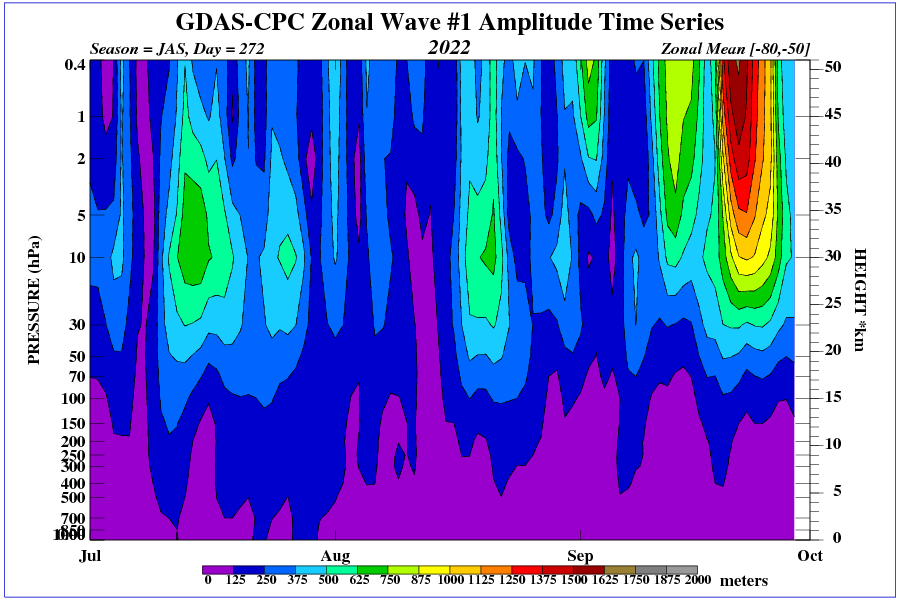
What do the current stratospheric temperature anomalies over the southern polar circle and the decrease in geopotential height tell us?
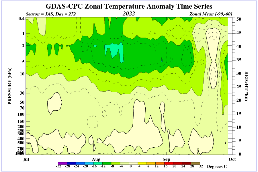
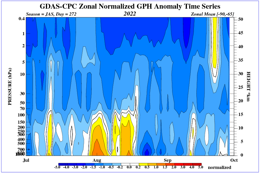
As the solar cycle progresses, the southern polar vortex strengthens.
The prolonged periods of weak solar wind (low velocity and temperature) seen in this cycle may affect the ripple of the jet current (whose pattern dynamically develops in the tropopause and reaches up to the 500 hPa level) over the Atlantic. The blockage of the zonal (westerly) circulation over the Atlantic has brought drought to Western Europe, and even the easterly circulation is seen periodically in Eastern Europe.

In North America, the circulation is typical of La Niña. La Niña can last up to the peak of solar activity (an increase in the strength of the solar wind over an extended period of time).

Reading the comments I was reminded of the ocean’s tides.
From first principles the tidal range should be something like 6 inches.
But because the forcing is in phase with a natural frequency the effects are much greater.
The Bay of Fundy for example being the correct length to turn 6 inches of forcing into 50 foot tides.
Tidal prediction isnt something that can be done the way climate models try and predict climate. That approach would not work.
The strong negative temperature anomaly of the western equatorial Pacific continues. Will the upcoming La Niña peak be the strongest?

QBO, did I miss what this stands for in the text
The Quasi-biennial Oscillation (QBO) is a tropical, lower stratospheric, downward propagating zonal wind variation, with an average period of ~28 months. The importance of the QBO is that it dominates the variability of the tropical lower stratospheric meteorology [Wallace, 1973]. The QBO is also important for seasonal forecasting, and the QBO controls stratospheric ozone and water variability that can modulate surface ultra-violet (UV) and infrared (IR) radiation.
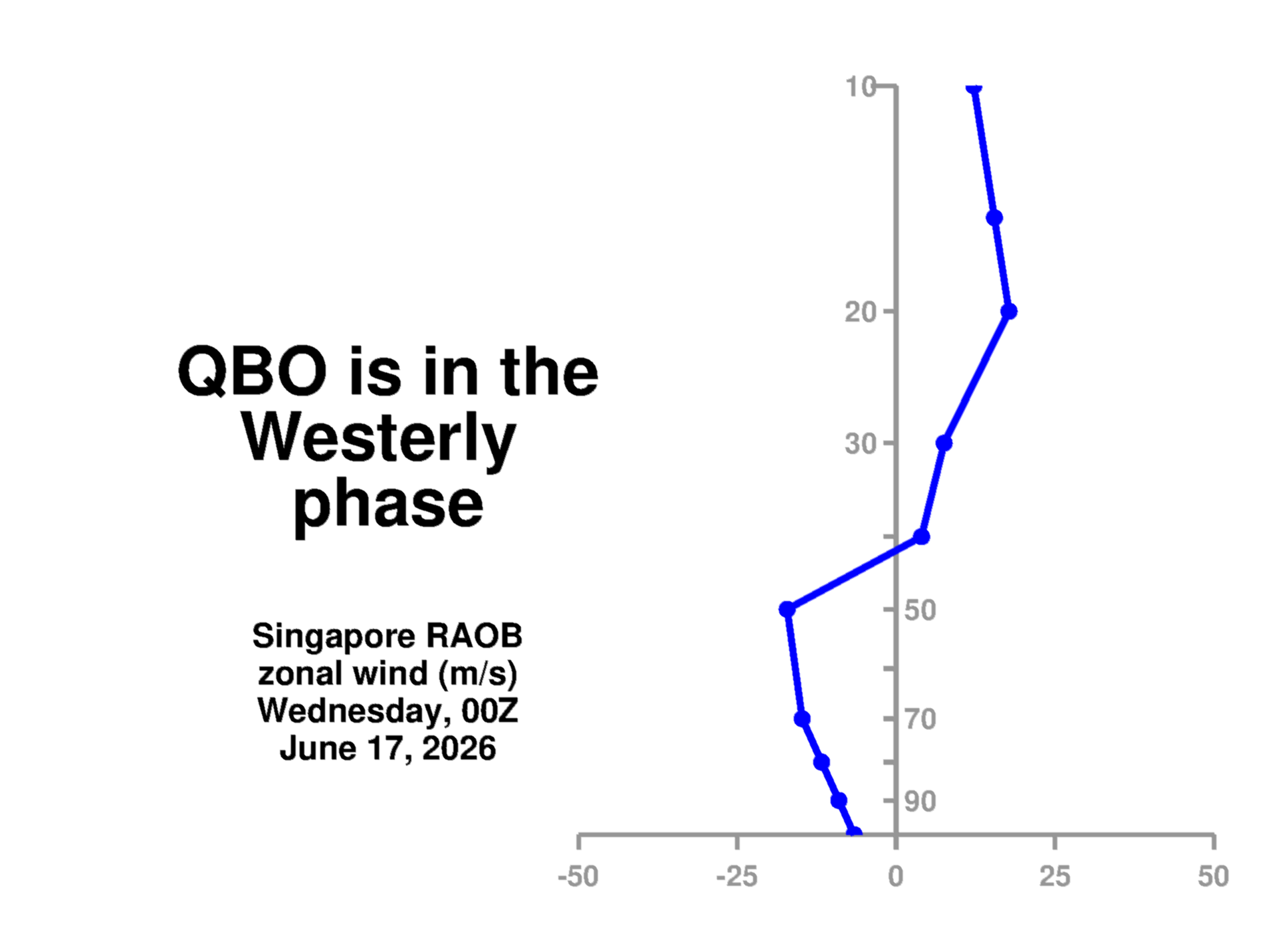
https://acd-ext.gsfc.nasa.gov/Data_services/met/qbo/qbo.html
I want to know more about the QBO. I find it interesting that it changes direction in a regular pattern.
I would love to see a video of how the QBO moves.
You missed the abbreviations-glossary document for the entire series linked at the end of every part.
Greeting Javier and Andy
Some basic questions.
1 – Is the total heat from oceans via convection measured annually ?
2 – What method is used to measure these volumes other than SST ?
3 – Does the volume vary annually ?
4 – Is there a variation in volume between the NH and SH annually ?
5 – Is the location of ocean heat release identified annually ?
Answer to these questions is – no one knows.
Facts
1 – The Zonal winds rotating around the poles are controlled by the level of convection at lower lattitudes.
2 – It is the strength of and convection volume and location that dictates the temperature anomaly variations.
3 – When you do research into the monthly regional anomalies you would find that the most prominent change in that location was wind direction.
4 – There are convection pulses that drive the anomaly variances.
Regards
Martin
Ask for my email address from WUWT and I will send you a draft copy that will identify what influences the temperature anomalies in strong convective years.
A slow increase in the strength of the solar wind’s magnetic field can be seen. Measuring the level of neutrons near Earth (secondary galactic radiation) is a very good indicator of magnetic activity in the solar disk.
