The first version of this post had an error in Figure 1. It has been fixed along with the associated text (7/5/2021).
By Andy May
The IPCC claims, in their AR5 report, that ECS, the long-term temperature change due to doubling the atmospheric CO2 concentration or the “Equilibrium Climate Sensitivity,” likely lies between 1.5° and 4.5°C, and they provide no best estimate (IPCC, 2013, p. 85). But their average model computed ECS is 3.2°C/2xCO2. Here, “°C/2xCO2” is the temperature change due to a doubling of CO2. They also claim that it is extremely unlikely to be less than 1°C. ECS takes a long time, hundreds of years, to reach, so it is unlikely to be observed or measured in nature. A more appropriate measure of climate sensitivity is TCR, or the transient climate response, or sensitivity. TCR can be seen less than 100 years after the CO2 increase, the IPCC claims this value likely lies between 1° and 2.5°C/2xCO2, their model computed average is 1.8°C/2xCO2 (IPCC, 2013, p. 818).
The CO2 climate forcing, or the net change in radiation retained by Earth’s atmosphere associated with these scenarios is 3.7 W/m2 (IPCC, 2007b, p. 140). Using these values, we can calculate a surface air temperature sensitivity to radiative forcing (RF) of 1.8/3.7 = 0.49°C per W/m2. These values are inclusive of all model-calculated feedbacks.
The IPCC explicitly state that they believe cloud, water vapor and albedo feedbacks are all positive and claim both model and observational evidence for this (IPCC, 2013, p. 82). They admit that cloud feedback, especially low cloud feedback, is poorly constrained and the source of most of the spread in model results (IPCC, 2013, p. 817). Cloud feedback is poorly understood; but it can offset the entire estimated human impact on climate. According to CERES satellite measurements, the net RF of clouds has recently varied from -13 to -25 W/m2 as shown in Figure 1. Both numbers are negative, which means that overall clouds cool the earth. If the IPCC claims that doubling CO2 will increase RF about 3.7 W/m2 at Earth’s surface are true, this is less than the change in yearly cloud RF. For more on clouds and global warming, see here.
The IPCC wants us to be concerned about a CO2-caused change about 100 years from now, when we see a larger change in radiative impact every year. Their computed impact of doubling CO2 is tiny compared to natural changes. The uncertainty in the impact of CO2 on climate is the difference between two tiny numbers, both too small to measure. One might reasonably conclude they have a screw loose.

It is worth repeating that the AR5 report does not provide a best estimate of ECS because of a lack of agreement in their various estimates. It is also significant that they think that TCR is extremely unlikely to be more than 3°C/2xCO2, but they do not offer a lower limit they are confident in. A summary of the IPCC estimates of ECS and TCR is presented in Box 12.2 of AR5 (IPCC, 2013, pp. 1110-1112).
There are several peer-reviewed estimates of climate sensitivity, based on observations in the real world, that are less than 1°C/2xCO2. These estimates are the focus of these posts. Some of these estimates are of ECS and some of TCR, or similar to the quantity that IPCC labels TCR. In this post we will not distinguish between the two. The IPCC has specific model-based definitions of ECS and TCR that do not translate to the real world. Here we focus on real-world estimates, not abstract model constructions. The IPCC tries to ignore these lower estimates and claims they are discredited (IPCC, 2013, p. 923), we think this is inappropriate.
The lower estimates come from Richard Lindzen (Lindzen & Choi, 2009), Sherwood Idso (Idso, 1998), Reginald Newell (Newell & Dopplick, 1979), and Willie Soon (Soon, Connolly, & Connolly, 2015). Lindzen’s estimate is about 0.5°C/2xCO2, Idso’s is 0.4°C/2xCO2, and one of Soon’s (he offers four) is 0.44°C/2xCO2. Newell and Dopplick derive 0.25°C/2xCO2 for the tropics. The researchers use a variety of datasets and methods, but all are observation-based. We will get into the details below and in a second post that will appear in a day or two.
There are other observation-based estimates, such as the well-known estimate by Nic Lewis and Judith Curry using historical CO2 and global temperature records. Lewis and Curry estimate TCR to be 1.2 (5%-95% range: 0.9-1.7) °C/2xCO2 (Lewis & Curry, 2018). Lewis and Curry’s work is excellent, but we will focus on the lower estimates in this post. We mention their work only to show that many, if not most, observation-based estimates of TCR are lower than the model-based estimates. Models that do not track observations should be ignored.
While AR5 does address Lindzen and Choi’s work, they ignore Idso’s estimate from 1998, Newell and Dopplick’s estimate from 1979, and Soon’s estimate was not yet published.
Lindzen and Choi
In a series of papers Lindzen and his colleagues have developed a robust hypothesis that rising sea surface temperatures (SST) cause some high-level tropical cirrus clouds to disappear, opening the sky so that more infrared radiation can escape into space, cooling the tropical atmosphere and surface. As mentioned above, the IPCC claims that net cloud feedback to warmer surface temperatures is positive and further warms the surface. CERES tells us that the overall impact of clouds is negative, but how cloud cover changes with surface temperatures is unclear. Lindzen’s investigation into this problem is illuminating.
Most tropical cirrus clouds, but not all, originate in the upper reaches of cumulonimbus towers. The hypothesis is that higher surface temperatures cause the precipitation efficiency within the cumulonimbus towers to increase, as well as the number of towers, therefore, there is less water vapor available high in the towers to form cirrus clouds (Lindzen & Choi, 2021). High-level cirrus block outgoing infrared radiation, but allow most incoming shortwave radiation in, so reducing cirrus covered area cools the surface.
Lindzen calls the reduction of cirrus cloud cover, due to rising surface temperatures, the “iris effect;” since it is analogous to opening an eye’s iris. This negative feedback is not part of most climate models, but Thorsten Mauritsen and Bjorn Stevens added it to their ECHAM6 climate model and found it caused the model’s results to move closer to observations (Mauritsen & Stevens, 2015). A one-degree increase in surface temperature reduces the cirrus cloud cover by 22% in the tropical Pacific, so it is significant.
The standard ECS, computed from the ECHAM6 model output, is 2.8°C/2xCO2. When the iris effect is added to the model, ECS always becomes smaller, and can fall to 1.2°C/2xCO2 in some scenarios. As mentioned above Lindzen computed an ECS of 0.5°C/2xCO2 from the cloud feedback parameter derived from ERBE (Earth Radiation Budget Experiment) satellite data. The precise impact of the iris effect has yet to be determined, but once incorporated, it always lowers both TCR and ECS.
Despite severe criticism over the past 20 years, including a paper entitled “No Evidence for Iris” in the Bulletin of the American Meteorological Society (Hartmann & Michelsen, 2002), the cooling iris effect is generally accepted today. What is still being debated is the magnitude of the effect. While in theory, the ECS can be computed from the total feedback, the calculation has many unknowns, these are described in Lindzen’s papers, especially the first one in 2001 (Lindzen, Chou, & Hou, 2001). Depending upon the assumptions made, Lindzen’s iris effect results in an ECS between the purely observation-based 0.5°C/2xCO2 (Lindzen & Choi, 2009) and the model-based 2.5°C/2xCO2 (Mauritsen & Stevens, 2015). While the range of possible values is large, they are all smaller than calculations that exclude the iris effect using the same assumptions.
Lindzen emphasizes that the cirrus cloud response to SST warming is essentially instantaneous, data lagged a month, or more are not usable and misleading. There are also factors other than SST that affect the area covered by cirrus clouds complicating the calculation. Statistically the longwave infrared (LW) feedback response to the iris effect is a reliable -4 W/m2K-1. That is, as SST goes up one degree, it results in 4 Wm-2 of LW RF cooling. But the loss of clouds also means more shortwave radiation (SW) hits the surface from the Sun, so the net amount of cooling is in doubt. The estimates in the increase of SW as a function of cirrus cloud cover are less precise than the cooling effect of escaping LW, but probably between 3 and 3.5 W/m2K-1. So, the exact amount of cooling due to the iris effect remains unknown, but there is general agreement that the iris effect exists, results in cooling, and reduces ECS and TCR.
Soon, et al., 2015
No one knows precisely how Earth’s surface temperature varies with insolation. Just like the weather, the energy flux at the top of the atmosphere changes, so long-term small changes, whether due to changes in the Sun, or the CO2 concentration, are obscured by short-term natural variability. Likewise, the surface temperature record has measurement problems, both systematic problems and instrument problems.
Willie Soon and colleagues were concerned that urbanization may have contaminated the global temperature network, so they created a record of Northern Hemisphere (NH) temperature using predominantly rural weather stations (Soon, Connolly, & Connolly, 2015). Their new record was compatible with NH SST trends and records of glacier advances and retreats. The record was combined with a NH SST record and compared to the Hoyt and Schatten TSI (Total Solar Irradiance) reconstruction as modified by Scafetta and Willson (Scafetta & Willson, 2014). The match was quite good as you can see in Figure 2.

The least squares fit of the curves in Figure 2 results in a set of residuals that is quite small. The R2 is 0.48 to 0.5 and the slopes are 0.1 to 0.211°C/Wm-2. Soon and colleagues assumed that the temperature variation that was unexplained by the change in TSI was due to increasing the CO2 concentration and, depending upon how they did the calculation, resulted in a climate sensitivity between 0.44°C/2xCO2 and 1.76°C/2xCO2 (Soon, Connolly, & Connolly, 2015).
The TSI reconstruction shown in Figure 2 is similar to many others, as shown in Soon, et al., but the IPCC generally ignores the more active TSI reconstructions and favors more invariant reconstructions that make it appear that CO2 is the dominant factor in recent warming. The key point is that the climate models are tuned to the various global temperature records, which may very well be contaminated by the rapid urbanization that took place in the 20th century. The tuned IPCC models of natural warming assume a nearly invariant Sun, so when the natural-only modeled temperature is subtracted from the anthropogenic plus natural model to extract the human (or CO2) component of warming, all the warming is assigned to humans and CO2. This IPCC process is described here. The post also displays plots of various peer reviewed TSI reconstructions, those used by the IPCC and those they ignore.
Conclusions
In this post we compare the IPCC view of climate sensitivity to two modern observation-based estimates that are lower. In particular the low-end of the ranges that Lindzen, Soon and their colleagues calculate are much lower than the low-end estimate by the IPCC, yet they are based on reasonable assumptions and observations.
In the next post we will look at older, but still valid, observation-based estimates of climate sensitivity. The next post will also investigate estimates of surface air temperature sensitivity to radiative forcing. One main point, is that the impact of doubling CO2 is tiny compared to natural changes. As you can see in Figure 2, very small changes in solar output, 4W/m2 or 0.3% of 1361 W/m2 can make nearly as much difference as all the CO2 emitted to the atmosphere by humans. Likewise, yearly observed changes in cloud RF are larger than the impact of human-emitted CO2. The impact of CO2 on climate is too small to measure, thus we are arguing and panicking over something that likely doesn’t matter.
Download the bibliography here.
How can there be a ECS for CO2 when there is no equilibrium? How can there be a TCR for CO2 when it always follows SST?
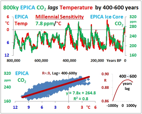
Endless repetition of inherently flawed ECS/TCR numbers for CO2 won’t change the facts.
“How can there be a TCR for CO2 when it always follows SST?”
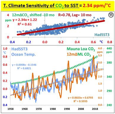
Always? Your graph says sensitivity of CO₂ to SST is 2.34ppm/°C. But CO2 is increasing at about 2 ppm/year. And the sea isn’t warming at 1°C/year.
The answer is, of course, that we are putting CO₂ directly into the air. That doesn’t follow any kind of temperature.
“And the sea isn’t warming at 1°C/year.”
It doesn’t have to. The sensitivity is for the 12mo change in CO₂, which doesn’t produce a constant 2.34 ppm/year as you implied because the SST changes vary each year, with no two years the same, leading to different ppm for each particular year, not a set “2 ppm/year’. The 2.34 value is an average over all variations.
I’ve done further work indicating the area and SST of the ocean at or above the CO₂ outgassing threshold temperature I derived of 25.6°C is a better metric than just the HadSST3 global ocean, an area that has grown significantly since the 1850s, along with decreasing area of CO₂ ocean sinking in colder waters than 25.6°C due to the overall warmer ocean.
“we are putting CO₂ directly into the air. That doesn’t follow any kind of temperature.”
Man-Made CO₂ emissions also lag Mauna Loa CO₂:

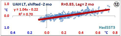
The ocean temperature sets the atmosphere temperature trend:
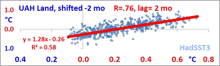
The ocean temperature sets the land temperature trend:
Therefore man-made emissions can’t control the climate.
Why should that be the case?
“Climate scientists” know nothing about the climate effects of clouds. They got it all wrong from the get go..
https://greenhousedefect.com/the-beast-under-the-bed-part-1
You should also look at Philippe De Laminat’s book Climate Change :Identification and Projection. In this book he uses system identification of 4 temperature reconstructions to determine the significance of solar input, CO2 concentration and volcanic activity. From these he has determined the sensitivity of temperature to each of the last 3 parameters. He finds that the temperature is very sensitive to solar activity and to major volcanic activity but relatively insensitive to CO2 Concentration (log of concentration as per the accepted theory). Using assumption free identification, the influence on temperature of solar activity was found to be several times greater than that of CO2 concentration and volcanic activity was marginal but not negligible.The relative figures for sensitivities were
CO2 doubling 1.28C/W/m2
Solar irradiance 17.5C/W/m2
Temperature was also highly sensitive to volcanic activity but had little overall effect on historical temperature because it is inconstant.
When these figures were used to predict temperatures for times after the identification had been done, it was found that the predicted temperatures were well aligned to the measured temperatures. Indeed when the sensitivity to CO2 was set to the mean value of the IIBCC (1.6C/w/m2) it was found that the predicted temperatures still aligned well with those that were measured. This is not surprising given that the identified sensitivity to solar irradiance is more than 10 times the IIBCC estimate for CO2 doubling.
The current reduction in solar output as we are in a solar minimum seems to me to be reflected very well in the current cold spell where global temperatures have dropped significantly in the last several years.
As a final note system identification is used to determine the sensitivity of the output of industrial processes to changes in input parameters. For example one could identify the outputs of a cement kiln such as the quality of the clinker with the input feed rate, fuel consumption, chemical composition of the feed etc. System identification is used to determine the significance of the parameters and to design control algorithms to produce a particular desired output.
Sounds very interesting, thanks!
I don’t care what anyone says. We have no idea what total solar irradiance was in 1860. No proxy would be able to evaluate that to any useful certainty. This is all voodoo science predicated upon believing infallibility of proxies.
“ECS takes a long time, hundreds of years, to reach” No it doesnt. Every day the sun comes up, and the surface tempresponds in a few hours to its forcing. And every afternoon it cools a few hours later as the forcing dies off.
If the sun went out within a few days the land surface would be below zero. In a few years the oceans would start to ice over.
The suggestion that todays high temperature is due to heat stored by a GH gas a few centuries ago is ridiculous.
It takes a long time for the ECS to play out because of the thermal inertia of the climate system. ECS does not complete until the Earth Energy Imbalance (EEI) is driven back down towards 0 W/m2. There is a lot of mass in the climate system so it takes a lot of energy to raise the temperature and drive OLR up thus reducing EEI. A lot of this energy goes into phase changes (like that of ice to water or water to vapor) or possibly increases in kinetic energy (like that of winds or ocean currents) which don’t result in a temperature increase and don’t reduce the EEI. Then you have the feedbacks to consider as well which can put more upward pressure on the EEI. It can decades, centuries, or even millennia (if slow feedbacks are considered) for the ECS to fully play out.
GHGs do not store energy in the way you are thinking. I mean they do store energy like any substance proportional to the amount of mass and the specific heat capacity. They just don’t store it in the way you are thinking here. The planet is not warming today because GHGs stored energy a few centuries ago and are just now releasing it. The planet is warming today because GHGs impede the transmission of energy to space creating a positive EEI. And as I glossed over above it can take a really long time for the EEI to stabilize close to 0 W/m2. What that means is that even if GHG concentrations stabilize at present day levels it will take decades or longer for the EEI to return to something close to 0 W/m2. In that context the GHG emissions from decades ago are still causing the climate system to accumulate energy.
Hand-waving.
Thanks, bdgwx. This exemplifies a common misunderstanding, that a top-of-atmosphere energy imbalance can only be rebalanced by surface warming. In fact, there are a number of ways it can be rebalanced.
First, of course, the amount of energy entering the system can be reduced by a relatively trivially small change in the albedo. This will happen if the amount, type, or timing of the emergence of the clouds changes.
Second, the amount of energy radiated out by the atmosphere is a function of the amount of energy absorbed by the atmosphere … and GHGs are only a part of that. There’s also the amount of sensible heat absorbed by the atmosphere, the amount of latent heat absorbed by the atmosphere, the amount of sunlight absorbed by the atmosphere, and the amount of advected energy that is absorbed in one location and radiated in another location. So a change in any of those can rebalance the energy budget.
Finally, thunderstorms move immense amounts of energy from the surface to the upper troposphere without interacting with CO2 in any way. From the surface to the inside of the thunderstorm it’s moved as latent heat, and from there it goes up the inside of the thunderstorm tower to the upper troposphere. In neither case does it interact with CO2. So an increase in the number, strength, and/or timing of the thunderstorm emergence can re-balance the budget.
In short, your idea that an energy imbalance can only be re-balanced by a long, slow process of the globe warming is simply not true.
Best regards,
w.
Yes, of course, I agree that energy balance can restored by a change in ASR as well like would occur with a change in albedo from ice or cloud coverage changes, aerosol changes, or solar radiation changes. The question is…which is a more likely pathway for a positive EEI to reduce back toward zero…a decrease in ASR or an increase in OLR? And a crucial if not related question is whether the cloud feedback is positive or negative? And based on the observation that OLR is increasing at least suggests that ASR may actually be increasing too keeping the EEI fairly stable. This means the cloud feedback could be positive. Or at the very least we cannot eliminate that possibility. Either way though I do think any feedback based on temperatures will play out slowly due to the thermal mass of the climate system. There is plenty of room to debate what “slowly” actually means…years…decades…centuries?
Let me repeat, if the sun when out the land surface would be ice in a few days and the oceans iced over in a few years.
Thats your inertia, right there, and it amounts to very little.
The fact is that even if it is 3 C warmer, like during the Holocene Climatic Optimum, when Climate Change consisted of the Sahara being green, it is beneficial.
Any warming within this ECS range, and increase in CO2 is beneficial. Climate Change is good, CO2 is good, green deserts are good, more plant growth is good, greater drought resistance in plants is good.
It is all good. We should produce a lot more CO2.