From the Friends of Science Society Newsletter, where they give our own Willis Eschenbach props and suggestions for his important recent work – Anthony
The Clouds and the Earth’s Radiant Energy System (CERES) project provides satellite-based observations of Earth’s radiation budget and clouds. CERES instruments on several satellites measure longwave and shortwave radiation from the Earth. The longwave radiation is the radiation emitted upward to space from the Earth’s surface and clouds. The upward shortwave radiation is the reflected solar radiation which doesn’t enter the climate system. If the outgoing longwave radiation is less than the absorbed solar radiation, there is a positive top-of-atmosphere radiative imbalance (imbalance) which increases the global average temperature.

Willis Eschenbach used the CERES database, which gives the monthly radiative fluxes in each 1° latitude by 1° longitude starting March 2000, to calculate the equilibrium climate sensitivity (ECS) to greenhouse gases. He produced a graph of imbalance versus the surface temperature by 1° latitude by 1° longitude with time averaged over 24 years. Eschenbach applied a lowess fit to the data. He calculated the slope of that fit and calculated the area weighted imbalance per degree of temperature change. Eschenbach asks “How much does the earth have to warm up to restore the 3.7 watts per square meter (W/m2) of TOA radiation imbalance that is said to result from a doubling of CO2 (2xCO2)?” Willis says the amount of warming required to rebalance the imbalance is called the ECS, but I believe that isn’t correct. The imbalance is not at an equilibrium state but is the result of a continual increase of greenhouse gases.
The transient climate response (TCR) is the change in temperature after a doubling of CO2 at a constant increase of a 1%/year, which would result in a doubling in 70 years. The actual average CO2 increase from 2000 to 2024 was 0.567%/year. Willis calculates the imbalance at 6.6 W/m2 per °C of surface temperature change. This equates to a TCR 3.7/6.6 = 0.56 °C, which is the TCR at 0.567%/year CO2 increase. I call this the “slowTCR”, to distinguish it from the normal TCR with a 1%/yr CO2 increase. Using a simple 1-D climate model tuned to 3-D models, with CO2 increasing at the actual rate, I calculated that the slowTCR of 0.56 °C corresponds to an ECS of 0.68 °C, which seem much too low compared to other observation-based estimates.
I did a similar calculation using the same CERES data. Each data point is 1° latitude by 4° longitude. I applied a 4th-order polynomial fit to the average 25-year data (16200 data points) as shown in this graph. I made another graph of the slope of the fitted curve and calculated a global average imbalance of 3.95 W/m2 per °C of surface temperature change, which corresponding to a slowTRC of 0.94 °C and an ECS of 1.14 °C. The lowess fit heavily discounts data further away from the mean to discount outliers. The polynomial fit might be better as all the data is of equally high quality. Changing the best fit method has a large effect on the results.
Several papers, see here and , here, argue that cloud cover can change due to atmospheric circulation changes caused by a temperature change. The analysis by Eschenbach and myself using time averaged CERES data doesn’t account for this possible effect and assumes that any potential temperature-caused air circulation changes will not significantly change the relationship between imbalance and temperature over the next few decades of climate change. Therefore, I did the same calculation using the four coldest years of the CERES data (2000, 2001,2008, 2011) and the four warmest years (2018, 2019,2023, 2024). The global average temperature difference between these year groups is 0.68 °C. If the air circulation changes were causing more warming, the result of the warm years would show a lower imbalance change per temperature change than the cold years. In fact, the warm years analysis has a slightly smaller change of 0.13 W/m2/°C, so it appears that this effect is leading to more warming. Therefore, the method we used to estimate ECS is likely inaccurate. It is not a simple task to estimate the ECS.
I know damn little about the science and equations used here but if these guys want to compare their work to Willis’ shouldn’t they use the same one degree longitude and one degree latitude that Willis used?
For “estimates based on observations” some other process would be needed. No thermometers exist to fill in the 1×1 blocks over the planet, so some version of what this site routinely lambastes as nonsense assumptions and regional uniformity is needed. ECS is degrees C per doubling. Actual, accurate, long term temperature measurements are not available for most of Earth.
The problem is easy to poke fun at and difficult to solve because there is not enough data to say much of anything (except the planet is estimated to be very old and shows no evidence I know of having runaway hot yet)
The figure is wrong.
The 1979 Charney Report presented an ECS range of 1.5 to 4.5 degrees C, with central value of 3.0 C, which became “canonical”.
Charney derived this from the first two GCMs of Manabe, whose model found 2.0 C., and Hansen, who computed 4.0 C. Charney added an arbitrary error margin of 0.5.
Based upon observations rather than GIGO models, Lindzen et al have shown ECS to lie in the range of 0.0 to 1.0 C.
There is plenty of scientific rational to support the conclusion that the climate sensivity of CO2 is effectiely zero.
Agree . . . and further comment that most calculations of ECS or even TCR do not properly account for the Beer-Lambert law “extinction coefficient”, aka linear attenuation coefficient, (see https://en.wikipedia.org/wiki/Attenuation_coefficient ) for greenhouse gases in Earth’s atmosphere, particularly that for CO2. Many notable scientists, particularly Prof. William Happer, have noted that at CO2 concentration levels above 300 ppm (and Earth’s atmosphere is currently at about 420 ppm global average), increasing levels of CO2 do not significantly increase the total amount of LWIR CO2 absorbs from Earth’s surface.
This is commonly referred to a reaching an asymptotic “limit” on a given physical effect, such as the limit for how much salt can actually be dissolved in a fixed mass of water at STP.
There most likely WAS a time long ago when variations of lower atmospheric CO2 concentrations did meaningfully affect atmospheric temperatures via the “greenhouse effect”, but that was then and this is now.
So there is really no sense in now discussing what “doubling atmospheric CO2 levels” might mean in terms of any associated, (mis)calculated effect on global temperature.
“The great tragedy of Science — the slaying of a beautiful hypothesis by an ugly fact”
— attributed to Thomas Henry Huxley
It take a very long time to double the amount of CO2. See this graph;
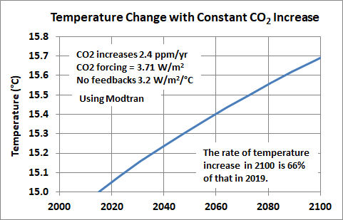
It shows that with a constant CO2 increase of 2.4 ppm/yr, which is the current rate, the rate of temperature change per year in 2100 is 66% of that in 2016. Climate models and Modtran take into account the CO2 logarithmic saturation effect. That effect is small over the time frame of interest to 2100.
Ahhhh . . . 66% of “essentially zero” is still “essentially zero”. That’s one of the great misunderstandings that results from carelessly applying a mathematical equation to physical processes, especially via “models”.
Besides which, there is no credible science evidence beyond a reasonable doubt that “CO2 forcing”, as noted on the graph you posted, is currently at 3.71 W/m^2. Consequently, this graph is GIGO.
The only way that adding CO2 to the atmosphere can cause warming of the Earth’s surface would be to increase the thermal insulation properties of the atmosphere. The temperature profile of the atmosphere is a measure of the atmosphere’s thermal insulation propertiues. A doubling of CO2 will cause a slight decrease in the dry lapse rate in the troposphere which is a cooling effect. Then there is the issue of H2O feedback. Because the wet lapse rate is significantly less than the dry lapse rate in the troposphere, the adding of more H2O to the atmosphere by evaporation from the surface has a net cooling effect and not a warming effect. Hence H2O must act as a negative feedback to any possible CO2 based warming. Negative feedback systems are inharently stable as has been the Earth’s climate over at least the past 500 million years, enough for life to evolve because we are here.
This is only partly true.
The temperature profile of the atmosphere, 99% comprised of the non-IR-active gases N2 and O2, directly indicates how efficient IR-active “greenhouse gases”, predominately water vapor and CO2, are in equilibrating LWIR energy emitted from Earth surfaces throughout the bulk of the atmosphere. They do this because the rate of their collisions with other atmospheric molecules is some 6 to 9 orders-of-magnitude faster than are their rates of photon re-emission resulting from their absorbed LWIR-photon-induced higher energy state (aka “photon relaxation time constant”).
This is the fundamental reason that molecules of water vapor and CO2 are found to have effectively the same temperature distribution as do nitrogen and oxygen at any given altitude in the troposphere, despite them temporarily absorbing LWIR energy.
BTW, long term (years to hundreds of years), the atmosphere only “insulates” Earth’s surfaces to the extent that TOA thermal radiation power (globally averaged W/m^2) balances the total incoming solar radiation (globally and temporally averaged W/m^2) that is absorbed by the atmosphere and Earth’s surfaces.
No, I am entiely correct. All gases in the Earth’s atmosphere are thermally active which is what really counts. Convection dominates over LWIR absorption band radiation in the troposphere. When a greenhouse gas malecule absorbs an LWIR absorption band photon it tauses thermalization, I slight increase in the apparent temperature of the molecule. That temperature affects the temperature profile. If adding CO2 to the troposphere really caused surface warming then we should see the effect in an increase in the dry lapse rate but instead adding CO2 to the atmosphere causes a very slight decrease in the dry lapse rate which has a cooling effect on the surface.
True, but I never stated or implied differently. Instead, I made a distinction between those atmospheric gases that were IR-active (water vapor and CO2) and those not IR-active (N2 and O2). Reading comprehension.
Not so. If there were no “greenhouse gases” to intercept and re-distribute LWIR surface radiation energy throughout the entire mass of atmospherice gases (predominately nitrogen and oxygen) then the direct escape of such radiation to deep space would result in much colder surface temperatures on Earth, likely below 32 deg-F, the freezing point of water. This is true independent of surface-to-atmosphere heat transport due to conduction, convection and enviro-transpiration (i.e., the hydrodynamic cycle of Earth).
FYI, Trenberth-type calculations of Earth’s “energy balance” (e.g., see attached diagram), indicate that only about 43% of Earth’s steady state-averaged net thermal radiation emissions to deep space involve conduction, convection, and enviro-transpiration processes transferring heat energy into the atmosphere from where it is then radiated to space. Atmospheric convection does not in fact “dominate over” direct LWIR surface-to-atmosphere-to-space transport when accurately accounting for all energy transport processes occurring.
This is an illogical statement, one commonly fronted due to misunderstand of the basic physics involved. Adding CO2 to the troposphere could only (hypothetically) cause additional surface warming to the extent the atmosphere first experienced additional warming (via “back radiation” coupling). In such a scenario, the atmosphere would, of course, warm more than the surface would warm and this would then lead directly to a “a very slight decrease” in the dry adiabatic lapse rate . . . there is no “instead” there.
Your self-declared
“No, I am entiely correct.” (with its misspelling)
is duly noted for what its worth.
About that Manabe GCM. It has the worst comparison to temperature observations, even in its current iteration.
I believe you directed this comment to the wrong person.
“Lindzen et al have shown ECS to lie in the range of 0.0 to 1.0 C.”
Lindzen works on the “radiative” theory.
Thing is, radiation is just a bit player when it comes to energy movement in the atmosphere.
David Dibbell has shown many times that bulk air movement transfers magnitudes more energy than any possible CO2 radiative effect.
Any mythical CO2 radiative effect is little more than a flea on the elephants posterior. !
Thanks for mentioning this. That “vertical integral of energy conversion” parameter from ERA5 certainly shows that the minor incremental radiative effect turns out to be vanishingly weak within the dynamic operation of the atmosphere. Here is a link to the Google Drive folder where this point is explained and supported with plots, histograms, and references.
https://drive.google.com/drive/folders/1PDJP3F3rteoP99lR53YKp2fzuaza7Niz?usp=sharing
Thanks for the Google Drive link, David. I’ve become a fan.
Considering the atmosphere as a heat engine (it was Carnot’s inspiration for the concept, BTW):
The “fuel” of the engine is sensible heat. This comes from three sources.
The “radiative equilibrium” models do not account for either 2 or 3. Either will destroy a “radiative equilibrium” which cannot exist in the Earth’s atmosphere. Schwarzschild’s understood this.
The “exhaust” of the heat engine is the radiation that escapes to space. Because the “atmospheric window” radiation does not interact with the atmosphere, it doesn’t add fuel and passes through. The radiation that escapes to space is not propagated through the atmosphere, it is generated by the atmosphere via collisions. The radiation can escape when the rate of spontaneous emission exceeds the rate of collisional de-excitation plus the rate of absorption. The H2O emission bands span the entire spectrum, and emit from the mid-troposphere to the tropopause. Look at an H2O only spectrum generator and this will be more clear. H2O accounts for almost all of the emission to space.
Ozone emits in the stratosphere.
CO2 captures a fraction of the water vapor emissions around the Q-band creating the “notch” centered at 667/cm. This absorbed energy is thermalized and returned to the “heat engine” energy pool. Emission from CO2 occurs near the mesopause and is represented by the tiny peak at the bottom of the “notch.” It is tiny because there is very little energy left to drive collisional excitation.
ERA5 captures the “work” of the heat engine. It’s a beautiful thing.
The transport of energy within the engine through the atmosphere is not via radiation, it is via convection. It is on the order of 10e-9 the speed of light. That is why the Earth is temperate rather than frigid.
The description above is for “clear skies”, of course.
The dynamics of the atmosphere cannot be captured vis a radiative model.
Tom
“The dynamics of the atmosphere cannot be captured vis a radiative model”
You are correct. However the dynamics of the atmosphere are very evident in the temperature anomaly method. In fact that’s pretty all that is being recorded.
The heat source / store is primarily the ocean, the ocean moves, the cloud determines where the heat enters the ocean etc etc, and the use of the anomaly method records where the heat went for the day, month, year. The UAH and other charts record this. Is the UAH chart Earth’s temperature ?. There is a strong argument for saying NO. And changing the base line every 3 to five years, really, the scientific method is not very scientific.
Regards
Martin
The average temperature/temperature anomaly as used in “climate science” is, for practical purposes, meaningless. First, temperature is an intensive quantity that applies only to the point where the measurement is made. I can create many different “average temperatures” in a space by the choice of locations and the number of measurements that I choose to make. Cohler discusses this in some detail here:
https://youtu.be/QRzAV8PVUws?si=ir2KURrDCHJbv_D8
Second, temperature is not a universal proxy for energy.
Thanks for your reply, Tom, and for being interested in the material I put together.
I would add to your numbered sources of heating of the atmosphere, that ~23% of incident solar energy is absorbed directly in the atmosphere without first being absorbed at the surface (from NASA as of 2009). So it’s a pretty big deal.
And that leads me to mention this reference about “horizontal heating gradients” as the main mechanism which produces the heat-engine-driven general circulation and maintains its overall kinetic energy state. See the first page of the pdf.
https://a.atmos.uw.edu/academics/classes/2010Q2/545/545_Ch_1.pdf
The rotating surface + atmosphere experiences incoming solar energy as daily pulses at each location, which implies a constant generation of those horizontal heating gradients. The Band 16 images help visualize the diurnal heating response.
There’s more to be said about the longwave radiation aspects, but suffice it for now to say that in any case the incremental effects from rising CO2 concentration, as computed from the widely used radiative transfer coding (e.g. RRTM-G), turn out to be entirely inconsequential to the climate system after properly considering the dynamics, as the “energy conversion” plots demonstrate.
Great description of a pulse. It’s not a square pulse normally used to obtain a transfer equation. That would solve a lot of issues in determining what is exactly occurring if we could actually do it. It is a sine shaped pulse which climate science never deals with..
I fully concur regarding the shortwave. I’ve been a bit myopic on the longwave side if you hadn’t noticed. My reference to convection is intended to include the coupled horizontal circulation as well.
And those flashes as insolation enters the picture in the Band 16 animations…CO2 emission is not effected by incoming solar. From cloud tops and deserts, that’s water vapor blooming and radiating, driven by collisional excitation. John Tyndall figured that out and wrote about it 150 years ago, though I expect few have read it. It’s the so-called “trapped” energy radiating to space.
It boggles my mind that the radiation “experts” haven’t figured out that above the clouds there is copious water vapor that can radiate to space, not part of a “clear sky” spectrum. The deserts likewise accumulate H2O near the surface at night. It flashes off in the morning.
Thanks for your further reply, Tom. Sorry for the delayed response here.
“And those flashes as insolation enters the picture in the Band 16 animations…CO2 emission is not effected by incoming solar. From cloud tops and deserts, that’s water vapor blooming and radiating, driven by collisional excitation.”
It makes more sense to me that the rapid daytime rise of the Band 16 “brightness temperature” visualized as yellow and red in the images is mainly the response of the skin surface to absorbed sunlight. This is strongest where there is little water vapor to attenuate the emission to space, as in the Atacama Desert.
While I understand your perception,
I will try to explain in more detail.
The perception that the desert is devoid of water vapor is common, but false. The lowest concentrations of surface water vapor are on the Antarctic plateau. Similar conditions can be found on high mountain peaks.
I’ll mention that in van Wijngaarden and Happer’s paper discussing the five most abundant greenhouse gases (2019, I believe) if you look at their spectrum for the Sahara Desert the water vapor concentration was 21000 ppm, 2.1 percent.
i live in the desert. As an example, this morning as I was enjoying my coffee, it was 80F and 29% RH. That corresponds to an absolute humidity of about 7 g/m^3 of water vapor. At 3 pm, the temperature is 107F, RH 8%. That’s about 2 g/m^3. In the desert, water tends to accumulate near the surface and overnight, and it begins to evaporate once morning insolation provides adequate energy.
This phenomenon has been studied in the Atacama. You can read this article where it describes this phenomenon.
https://blog.uni-koeln.de/awares/2024/04/25/the-paths-of-moisture-in-the-atacama-desert/
The concentration where IR active molecules can actually radiate to space is quite low. For the Q-band of CO2 at 15 microns which radiates in the mesosphere, the concentration would be comparable to less than 1ppm at the surface. Expressing concentrations in ppmv (relative) makes this less than obvious. The reason for this is that at higher concentrations re-absorption by neighboring molecules becomes a limitation factor.
Water vapor does not emit until the mid troposphere because the concentration is too high at lower altitudes. Condensation, which controls the lapse rate, also reduces the concentration of free water molecules, and only the free molecules can radiate to space. Any “blooming”of water vapor from the surface will, above a critical altitude, radiate to space.
GOES band 16 looks at a window of 13-13.6 microns, about 735-770/cm. This is on the right shoulder of the CO2 notch, between the bottom
of the CO2 “divot” and the atmospheric window.
I don’t know MODTRAN’s capabilities. I use NASA’s Planetary Spectrum Generator (PSG). If you look at this region in high resolution, it is a combination of minor CO2 bands and H2O bands. On PSG you can also look at the separate contributions of the two components. The CO2 concentration is constant. What will change the overall amplitude of the signal is a change in the concentration of water vapor.
Tom, Band 16 includes the near-black-body radiation from the rapidly warming solid surface, which will warm and emit much more, and more quickly, than the air above it. So it makes good sense that most of the rapid rise is because of the solid surface. Same idea for the rapid decay late in the day.
Be well. Lots to think about.
Here’s what UChicago Modtran says the 2x C02 warming at surface will be for clear sky, equatorial, humidity adjusted for ground level temp conditions…so worst case…1.21 C…so try runs at some cloudy conditions, add in some temperate zones till you get an average TOA of about 240 Watts/sq.M like the average of Planet Earth….and Voila…ECS somewhere around 0.7
The Earth’s atmosphere is governed by air movement not radiation.
The transfer of energy but bulk air movement totally dwarfs any radiative effects as to make them absolutely insignificant.
The only way that energy can significantly leave the planet is by radiation.
Only at the extremities.
All energy movement within the troposphere is governed by air movement.
When you use Modtran’s clouds, rain, humidity, locality, surface temp offset features…. these are parameterized quite well to match the various weather balloon models you are suggesting. Please provide the name of one such model we can run to compare.
“When you use Modtran’s clouds, rain, humidity, locality, surface temp offset features”
But not bulk air movement.
Balloons show that the atmosphere follows the gas laws.. ie bulk air movement.
CO2 is a gas and is governed by the gas laws.
H2O is not always a gas in the atmosphere, but is also a large part of bulk air movement.
Obviously parameterizations include “average” bulk air movement. That’s why various “localities” are included in Modtran…modifying the lapse rate primarily.
Anyone who has flown model gliders as I have will attest to the power of thermals on a sunny day.
Do the models incorporate the dominant effect of convection in atmospheric heat transport? I sincerely hope so since such models are utterly worthless otherwise.
CS is an abstraction not a prediction of reality. Like how far you can throw a feather in a vacuum. In reality the CO2 concentration does not determine the temp so CS does not exist. Moreover the weather system that climate is the average of is a far from equilibrium system so ECS is not even meaningful. The system cannot equillibrate.
Of course. The atmosphere is chaotic, and the Earth itself has cooled from the molten state – slowly continuing to do so.
To your point, “CO2 concentration does not determine the temp” – I am still impressed with how Sir George Simpson and Professor David Brunt explained this to Guy Callendar in their comments to his 1938 attribution of reported warming to rising concentration of CO2. More here.
https://wattsupwiththat.com/2025/04/06/open-thread-138/#comment-4058322
One of my favorites as well.
The good old days when meteorologists understood weather was a thermodynamic process, not a radiative process.
ECS and TCR definitions can only be realized in a computer simulation. However, we are using real data to estimate what those values are. If one has a good estimate of the value, it can easily be used to make reasonably good short term prediction of the temperature change effect of increasing greenhouse gases using only a simple 2-box 1-D model. CO2 changes DO affect temperatures by causing an radiative imbalance at the top of the atmosphere. More energy entering the climate system than leaving results in the difference accumulating in the climate system, thereby increasing temperatures. However, the rate of temperature increase is small the the effects are mostly beneficial!
The question is rapidly becoming – How many different ways can we torture the data to get the results we want?
Let me count the ways?<g>
When I searched “ECS” on WUWT, it came back with 30 pages of articles. 🙄
Per awful wikipedia: “Watts Up With That? (WUWT) is a blog promoting climate change denial that was created by Anthony Watts in 2006”
That’s 19 years of commentary by dozens of writers and millions of readers, with ECS being a central discussion point and here we still are with similar range and uncertainty. Rather than “what new way do we have to look at the data?” one has to start asking “what new data are we looking at?”.
“Per awful wikipedia: “Watts Up With That? (WUWT) is a blog promoting climate change denial that was created by Anthony Watts in 2006””
You get that same kind of negative comment about WUWT from Artificial Intelligence searches incorporating WUWT in the search. The AI’s sound just like Climate Alarmists. No doubt, they got some of their “training” from Wikipedia.
The science seems to have become – How many different ways can we torture the data to get the results we want? at least 25 years ago. The pioneers of this form of data torture have been selling their knowledge to undergraduates since then, because data torturers also have bills to pay.
There will be a generation of bitter middle class ecologists if the jig is finally up.
True. The presence of an atmosphere results in lower maximum temperatures, and reduced diurnal variations compared with the airless Moon, as it prevents about 30% of the Sun’s radiation from reaching the surface, whilst slowing the rate of nighttime cooling.
Increasing the proportion of either CO2 or H2O in the atmosphere exacerbates both effects.
Additionally, climate is just the statistics of weather observations, so talk of “climate sensitivity” is just meaningless word salad, uttered by those who should know better (no offense intended, the misuse of the term ECS is widespread, and rarely challenged).
As to any notion notion of “global warming” occurring as a result of the mythical GHE, I can only point out that no consistent and unambiguous description of this fabulous creature exists (unlike the the unicorn, say). Once again, a fairytale designed to impress the ignorant and gullible, put about by those who have no idea about reality.
People can choose to believe whatever they like, of course. Maybe I’m wrong, and we are all about to be fried, roasted, toasted and grilled unless we mend our evil CO2 ways, retreating to pre-Neolithic times, where we can all starve, while we freeze in the dark!
Who knows?
Graph links do not work. I get an error message.
Seem okay to me.
There is plenty of scientific rationale to support the conclusion that the climate sensivity of CO2 is effectively zero. For example adding CO2 to the troposphere actually slightly decreases the thermal insulatting properties of the atmosphere which is a cooling effect. Because the wet lapse rate is significantly less than the dry lapse rate in the troposphere, adding H2O to the atmosphere through any CO2 based warming would have a cooling effect. Hence H2O must act as a negative feedback to any posisble CO2 bassed warming. It is well known that negative feedback systems are inharently stable as has been the Earth’s climate for at least the past 500 million years, enough so for life to evolve because we are here.
“where they give our own Willis Eschenbach props”
Not really. He says:
“Willis says the amount of warming required to rebalance the imbalance is called the ECS, but I believe that isn’t correct. The imbalance is not at an equilibrium state but is the result of a continual increase of greenhouse gases.”
He’s right, and right again when he says:
“Therefore, the method we used to estimate ECS is likely inaccurate. It is not a simple task to estimate the ECS.“
These methods based on short term, local observations ignore the E in ECS.
The addition of CO2 into the atmosphere is far too slow to show measurable upset in the equilibrium. In that sense, the atmosphere would be in ”equilibrium” or ”balance” at all times. In other words, it’s all academic waffle.
The main disequilibrium is the time it takes to warm the sea.
Mr. Stokes: So the warming from CO2 that causes negative outcome is the heat moving from the low atmosphere into the sea?
No, that movement delays warming. But not forever.
Mr. Stokes: Doesn’t the “delay” you describe diminish and delay the negative effects of AGW?
That argument would rely on the ocean covering a large part of the surface under a liquid with huge heat capacity relative to the air that reflects, circulates, expands and evaporates.
Due to a side effect of saturation and the mechanisms of the boundary layers, CO2 cannot warm the surface (which includes “the sea”). It violates the 2nd Law. Why do climate cultists always deny basic physics?
Probably because they won’t keep getting paid if they start accepting basic physics…
“The second law of thermodynamics essentially states that in any natural process, the total entropy of a system and its surroundings will always increase. This means that the disorder or randomness of the universe tends to increase over time. A key aspect of this law is that heat will not spontaneously flow from a colder region to a hotter region.”
Heat goes from hot sun into cold space as radiation.
Radiation carries heat from cold space to warm earth.
Net transfer is from hot sun to warm earth.
2nd law says as long as earth remains colder than the sun, the sun will keep trying to warm it. Trouble is:
Heat goes from warm earth into cold space as radiation.
Radiation carries heat from cold space to warm ?.
Net transfer is from warm earth to ?.
Result in _a_long_time_ would be sun, earth, space, ? all getting cold like space.
As an aside, Google AI’s summary of standard language shows how math gets sloppy when translated to language. Who decides what a “natural process” is except to say it would violate the rule. e.g. All red herrings that are red must be red. Also “essentially states”: Can one state a thing “unessentially”? Maybe that’s what comment sections are for.
Between the Sun at 5800K and outer space at 3 K and the transparency of the atmospheric widow between 8 and 14 microns….there are lots of available phenomena for surface heating and cooling in our world that don’t break the 2nd law….just sayin’…
And the 30 years +/- it takes for ocean currents to mix the surface water and the 500-800 years it takes to mix the deep waters, and the unknown number of years it takes fresh water rain and snow melt to affect the halocline in any given ocean basin.
When has the Earth ever been at equilibrium? I would suggest never.
What is the exact scientific definition of ECS Nick ?? Is there one ??
According to WUWT (this article):
“Equilibrium climate sensitivity (ECS) is a measure of how much the Earth’s global average surface temperature will eventually increase in response to a doubling of atmospheric carbon dioxide concentration. Image by Anthony Watts”
The definition is WRONG
ECS is not a “measure”.. has never been measured….. it is a fantasy
As long as nothing else changes. But it does.
Look! A squirrel!
“E” is always trying to established itself by bulk air movement.
CO2 is a total zero when it comes to “E”.
If it weren’t for bulk air movement, (and subsidies) wind turbines would not exist.
… and they are correct to do so.
As the IPCC put it way back in 2001, on page 91 of the WG-I assessment report for the TAR, and has not seen fit to “correct” since then :
The real-world “Earth’s Climate System” is not now, has never been, and will never be, in an “equilibrium” state.
.
ECS is a derived parameter from “2xCO2” (and/or “4xCOZ”) model runs.
In the AR6 WG-I assessment report the IPCC made the following observation in Box 7.1, “The energy budget framework – forcing and response”, on page 933 :
In AR6 the IPCC also checked just how (in-)accurate those various models were against actual measurements (20th and 21st century) and GMST proxies believed to be relatively accurate for paleo-climate reconstructions.
A copy of Figure 7.19 from page 1009 of the AR6 WG-I report follows (hopefully, with the caption added manually) :
Figure 7.19 | Global mean temperature anomaly in models and observations from five time periods. (a) Historical (CMIP6 models); (b) post-1975 (CMIP6 models); (c) Last Glacial Maximum (LGM; Cross-Chapter Box 2.1; PMIP4 models; Kageyama et al., 2021; Zhu et al., 2021); (d) mid-Pliocene Warm Period (MPWP; Cross-Chapter Box 2.4; PlioMIP models; Haywood et al., 2020; Zhang et al., 2021); (e) Early Eocene Climatic Optimum (EECO; Cross-Chapter Box 2.1; DeepMIP models; Zhu et al., 2020; Lunt et al., 2021). Grey circles show models with ECS in the assessed very likely range; models in red have an ECS greater than the assessed very likely range (>5°C); models in blue have an ECS lower than the assessed very likely range (<2°C). Black ranges show the assessed temperature anomaly derived from observations Section 2.3). The historical anomaly in models and observations is calculated as the difference between 2005–2014 and 1850–1900, and the post-1975 anomaly is calculated as the difference between 2005–2014 and 1975–1984. For the LGM, MPWP and EECO, temperature anomalies are compared with pre-industrial (equivalent to CMIP6 simulation ‘piControl’). All model simulations of the MPWP and LGM were carried out with atmospheric CO2 concentrations of 400 and 190 ppm respectively. However, CO2 during the EECO is relatively more uncertain, and model simulations were carried out at either 1120ppm or 1680 ppm (except for the one high-ECS EECO simulation which was carried out at 840 ppm; Zhu et al., 2020). The one low-ECS EECO simulation was carried out at 1680 ppm. Further details on data sources and processing are available in the chapter data table (Table 7.SM.14).
.
Note the tendency for “hot” (ECS > 5 [ °C per CO2 doubling ] ) models to be outside the “observations” ranges while the “cool” (ECS < 2) models tend to be within those ranges, especially against the recent “empirical measurements with actual thermometers / thermistors” numbers.
Any parameter derived from the climate models, especially the “known to run hot” CMIP6 ensemble, should be taken with a very large pinch of salt.
“Therefore, the method we used to estimate ECS is likely inaccurate. It is not a simple task to estimate the ECS.”
This statement holds only if there is a positive significant cloud feedback to GHG radiative forcing – which is by no means certain. The two references cited by the authors certainly don’t demonstrate this.
The fact is, CERES data shows that most or all of the warming post 2000 has been caused by a reduction in earth’s albedo due to low level cloud cover changes, particularly tropical marine cloud cover. So if we are to attribute all or even most warming post 2000 to GHGs, then the positive cloud feedback due to a negligible direct radiative warming must be orders of magnitude greater than the radiative forcing itself, which to me sounds absurd.
It is rather more likely that, quibbles aside, TCR and ECS are very much lower than models suggest (<1.5C) and in fact decadal, perhaps even centennial variations in total cloud cover are principally due to internal variability and/or solar/volcanic forcing. The Hunga Tonga eruption in Jan 22 is a likely cause of the acceleration of penetrating short wave solar radiation due to the disruption of global circulation (dynamics) caused by the injection of the unprecedented amounts of water vapour into the stratosphere. We don't need an unanticipated acceleration of cloud feedbacks from GHG warming to explain the sudden spike in warming 2023/24, which is now rapidly fading.
All the temperature data sets used to guage ‘pre-industrial’ temperature normals already show in the region of ~1.3C temperature rise from 1901, and no sign of any reduction in the long-term rate of warming (0.2 – 03 C/dec).
The suggestion that there’s only a further ~0.02C at most to come in total is already risible.
“long-term rate of warming “
The biggest problem is that your definition of “long-term” is not really long-term at all. Some of the periods on earth with the greatest abundance of life had CO2 levels much higher than today. Where and how are these included in your “long-term”? Once of Freeman Dyson’s main criticisms of the climate models was that they are not holistic at all. They simply don’t consider the positive impacts of higher CO2 (and perhaps temperature) at all. The assumption of climate science is that higher temps are *bad*, totally and utterly *BAD*. No justification for the assumption at all. No holistic analysis at all. Climate science is just like Teyve in “Fiddler on the Roof” – the old ways are best, change is bad.
I’m not saying warming is good, bad or indifferent; just that it is a thing.
By long-term rate of warming I refer to the most recent 30-years, which across the surface data sets averages to +0.23C per decade.
So at that rate, assuming no further acceleration, we will fly past 1.5C above pre-industrial in about a decade.
Whether anyone considers that detrimental or beneficial or otherwise, it hardly supports the idea the ECS is less than 1.5C.
Your logic is based on an assumption that warming from pre-industrial times is BAD. What would your logic say if temperatures higher, maybe several degrees higher, is the optimum temperature? Should we be subsidizing additional CO2?
Don’t ask counterfactual hypotheticals. It makes their brains explode.
None of the warming in the last 45 years is from enhanced atmospheric CO2
If you think it is then show us the CO2 warming in the UAH data.
You have failed completely so far.
It is not that hard, but one needs to know the basics. And if you know them and read stuff like this, there are lots of “fingernails on chalkboard” moments.
There is no way to get 3.7W/m2 like this. Well actually there is, if you remove all other GH-agents, only keep CO2 and then double it, it gives you about 3.7W/m2 TOA. One can try that out in modtran. But that is only because there are no more overlaps with other GH-agents, mostly clouds and WV.
https://climatemodels.uchicago.edu/modtran/
With clear skies, thus no overlaps with clouds, you will get 3W/m2. Again, everyone can test that out on modtran, or read Wijngarden, Happer. Not a secret. With clouds (and their overlaps) eventually this figure drops by a 1/3, so that you get ~2W/m2. Not hard to do, if you know what you do, still Wijngarden, Happer did not manage to do it, although Wijngarden hinted to the 2W/m2 figure in his Tom Nelson interview.
“Consensus science” names 3.7W/m2 based on “radiative fluxes” at the tropopause, NOT TOA!!! So their calculation consists of 2.4W/m2 less upwelling there, and 1.3 more downwelling, sums up to 3.7W/m2. Already in SAR you have this definition:
I explained it all 2 years ago already..
I haven’t had tome to totally read and digest your link. I will note some things that jumped out at me.
I don’t find anything wrong with your paper, at least on the surface. At the very least it shows just how badly climate science analyzes the biosphere by making so many simplifying assumptions that violate physical reality.
“Heat loss from earth is higher during the day than it is at night because the temperature is higher when the sun’s insolation is intersecting the earth.”
Really! The Sun’s insolation intersects the Earth 24/day!
It’s not daytime 24 hrs per day.
Bah, but it is 5 o’clock somewhere.
It is now at the North Pole! Of course I wasn’t referring to a specific location on the Earth but the Earth as a whole and my statement was correct!
It may be, but the absorption at an angle of, let’s say 80°, is about (1370)(cos 80)(0.7) = ~ 167 W/m². ==> ~40C. Not much heat from the sun.
Don’t forget to multiply by 24 hrs!
Don’t need to. The SB equation will provide an instantaneous temperature value. Any point at 80° latitude will receive the same amount.
Nighttime lack of insolation also intersects the earth 24/day!
Phil thinks the Earth is flat.
No, I know it’s spherical which is why the Sun’s insolation intersects the Earth 24 hrs per day! The author of the paper referred to appears to think the Earth is flat though.
At any point on the Earth, the temperature goes UP less than 12 hours per day. The temperature goes DOWN more than 12 hours per day. This means that any point on the Earth spends more time losing heat than it does in gaining heat. It isn’t a matter of the period of daylight, it’s a matter of how much insolation is received. While in Chicago daylight is about 18 hours during the summer, it’s maximum temperature (determined by the insolation-in vs heat-out) is less than in Dallas which is closer to the equator and thus gets more insolation from the sun.
The sun follows a daily path located between the Tropic of Cancer and the Tropic of Capricorn. That path defines the path of maximum insolation from the sun. All locations not on that path always receive less than maximum insolation.
It’s why the GAT is such a joke. If you *really* want an average temperature for the globe then just use measurements from the 60° latitudes where cos(60°) = 1/2.
This was the quote I was referring to, it’s about the Earth as a whole not specific locations!
“Heat loss from earth is higher during the day than it is at night because the temperature is higher when the sun’s insolation is intersecting the earth.”
As I pointed out, the Sun’s insolation intersects the Earth 24/day!
By the way, what was meant by this?
“~ 167 W/m². ==> ~40C. Not much heat from the sun.”
40ºC in the North of Greenland would be very hot!
Blame my old eyes. I meant for it to say ~-40C.
You need to elucidate what you think this means. Show some math.
To me, under simple conditions, i.e., perfect sphere, the sun is always at the equator, etc., all that means is that every point on earth and at the same latitude will receive a similar amount of insolation. The insolation starts at sunrise at any given point, peaks, and falls to zero at sunset, a sine function from 0 to π.
As you move away from the equator the amount of insolation is also controlled by a cosine function from 0 to π/2.
There are many complications to deal with in the real world like a tilted axis, an oblate spheroid, and various and sundry variables. However, the basics are still there.
I don’t know what the sun shining 24 hours a day as the earth rotates has to do with the temperature profile at any given point.
Blame my old eyes. I meant for it to say ~-40C.”
Where did you get -40ºC from?
The Stefan-Boltzmann equation. Remember, this is only an estimation. I don’t claim it is entirely accurate, hence the approximate symbol.
(167 ÷ 5.67×10⁻⁸)¹/⁴ – 273 = 233 – 273 = -40
That gives you the temperature of a blackbody that emits that amount of heat. It’s certainly not a good approximation of the local temperature! Take for example the Freya glacier situated at about 75ºN, the webcam shows steady melting throughout July, most days were sunny and temperature was above 0ºC every day, most highs were over 10ºC (and that’s at ~1,000m altitude)!
Those are very nice temperatures. But you don’t mention what the surface temperature was. You don’t mention the albedo at that location
I do know that is a black body calculation. Remember I said it is only an estimation.
Air movement can have great effects on air temperatures. Do you have access to surface at the 5 cm depth? That would be enlightening. It is hard to believe that the surface is at 10ºC, since it melt ice quite rapidly.
Lastly, you haven’t addressed how much insolation is actually reaching the ground which is what I was addressing.
Well the ice there has been melting quite rapidly, here’s what it looked like about a week ago:
https://forum.arctic-sea-ice.net/index.php?action=dlattach;attach=384915;image
And a couple of weeks before:
https://forum.arctic-sea-ice.net/index.php?action=dlattach;attach=524257;image
The first image was the wrong date, here’s one from a couple of days ago:
https://www.foto-webcam.eu/webcam/freya1/2025/08/02/1030
“As I pointed out, the Sun’s insolation intersects the Earth 24/day!”
And again, so what?
With regard to Anthony’s figure, in the current Open Thread I discussed several models based on boundary values. If GHGs raise only the surface temperature, a 3.7W/m2 flux increase requires an 0.844±0.045K surface increase. If both tropospheric boundaries are equally increased 3.116±1.254K. In the first case the lapse rate is GHG dependent. In the latter, it is fixed as if by Convective Equilibrium.
“In the latter, it is fixed as if by Convective Equilibrium.”
As it is. DALR=-g/Cp. Nothing there about GHG.
Gee, Nick I think the A in DALR stands for AIR and a component of AIR is CO2 which has been named as a GHG. And D is DRY and dry air can contain a % of H20 which is also a GHG.
No, the A in DALR stands for Adiabatic.
And indeed the formula for it is -g/cp.
g= 9.81 m/s^2
Cp= specific heat of air = 1.005 kJ/kg·K
Precisely. CO2 does not affect the natural cooling gradient..
No atmospheric science of the cooling lapse rate contains a component from CO2.
H2O yes.. but not CO2.
No, the A in DALR stands for Adiabatic.
And indeed the formula for it is -g/cp.
g= 9.81 m/s^2
Cp= specific heat of air = 1.005 kJ/kg·K
-g/cp is a simplification of ideal gas law formulae that have a “gamma=Cp/cv” in them. Technically speaking CO2 is not an ideal gas and shows radiation absorption and emission effects that slightly affect “gamma”…nowhere near as much as water condensing though….
Why is it always about the sun’s energy and never the energy of the Earth?
Leo AI says this:
The temperature of the Earth itself has a significant effect on the temperature of the atmosphere. Here’s a brief explanation:
The average temperature of the atmosphere is 14C according to Wikipedia (yes I know).
Seems to me then that any Greenhouse Effect if it exists is of no concern and basically the atmosphere is cooling the Earth like anyone within 3 seconds of thought would have concluded since space is extremely cold.
Please don’t push AI stupidity.
The central climate issue is ECS, even tho it is a concept not a thing.
Guy Callendar’s famous 1938 curve implies 1.68. All the century long EBM studies produce a range around about 1.7. The only CMIP6 model that does NOT produce a spurious tropical troposphere hotspot (INM CM5) produces 1.8. The shorter term CERES stuff produces a significantly lower number, as does the Bejan constructal model. Willis Eschenbach has covered both of those.
The only ECS estimates suggesting a future problem are climate models that provably run hot, and provably produce a spurious tropical troposphere hotspot.
Ergo, we should call off the climate alarm.
Harold The Organic Chemist Says:
ECS is zero and is so much nonsense!
Shown in the chart (See below) is plot of the annual average temperatures at Adelaide which shows a cooling from 1857 to 1999. In 1857, the concentration of CO2 was probably ca. 280 ppmv (0.55 g CO2/cu. m) and by 1999, it had increased to ca. 370 ppmv (0.73 g CO2/cu. m.), but there was no increase in surface air temperature as might be expected due the increase in the concentration of CO2. Thus, it can be concluded that CO2 has little or no influence on surface air temperature and ECS is zero. Please note that there is very little CO2 in the air.
The Chart was obtained from the late John Daly’s website: “Still Waiting For Greenhouse” available at:
http://www.john-daly.com. From the home page, page down to the end and click on “Station Temperature Data”. On the “World Map” click on region or country to access temperature data from over 200 weather stations which show no warming up to 2002. Be sure to check the charts for all the weather stations in Oz, and especially the chart for Boda Island.
PS: If you click on the chart, it will expand and become clear. Click on the “X” in the circle to return to comment text.
Lowess is one of many types of regression. Regressions are designed to use an independent variable and a dependent variable. Neither temperature nor CO2 concentrations plotted using time as an independent variable will provide any relationship between the two. A relationship should provide a smaller and smaller range of possibilities.
One only needs to plot each on the same graph to see that there are other variables at work.
Who is the author of the text of this piece?
I am, Ken Gregory! You can click on the link to Friend of Science Society at the top of the article, then click “Contact Us”, or email me directly at kbgregory3 at gmail dot com. The article is here , 4th item CliSci #434 of 2025-07-27.
I can complete the analysis by adding the difference in the TOA imbalance-temperature relation between the warm and cold years group, which accounts for temperature caused air circulation changes, to the rate of imbalance change implied by the relationship of local imbalance to surface temperature of the 25-year analysis. The 25-year analysis gives an ECS of 1.14 C with a global average imbalance relationship of 3.95 W/m2 per °C. However, the imbalance difference between warm and cold years is -0.13 W/m2/°C with a temperature difference of 0.68 °C, equating to -0.19 W/m2/°C for a 1 degree temperature difference. Combining these gives 3.95 – 0.19 = 3.76 W/m2/°C. This give a slowTCR of 3.71/3.76 = 0.983 °C. My I-D model shows that is equivalent to an ECS of 1.20 °C. I don’t know how the recent reduction in aerosols (China cleaning up aerosols from its coal-fired plants and clearer fuel used in shipping) and the 10% increase of water vapour in the stratosphere due to the Hunga Tonga-Hunga Ha’apai volcanic eruption would affect this result.
This result [ECS of 1.20 °C] is very close to my estimate based on correcting the Lewis-Curry 2018 ECS estimate for the millennium climate cycle and the urban heat island effect, see here. Lewis-Curry-2018 gave an ECS best estimate of 1.66 °C. That analysis was deficient as it failed to take into account the millennium cycle (natural recovery from the Little Ice Age) and the UHIE. It is improper to ignore two well established known effects that would cause a significant change to the results of their paper. I asked Judith Curry to publish my results, a correction to Lewis-Curry-2018, which determined a ECS best estimate of 1.19 °C with a likely range of 0.90-1.57 °C. Curry rejected my article writing 2021-05-29; “Hello Ken, I’ve read this more closely. I think you use a value of ECS that is far too low. LC is already very low, at the bottom end of what people are willing to accept as plausible. The Gregory values look much too low.” She didn’t explain who are the people not willing to accept the result or why this should have any bearing on her decision not to publish it.
Ken Gregory
Harold The Organic Chemist Says:
ATTN: Ken
RE: Saturation of CO2 IR Absorption.
You should download:
https://climateatglance/carbon-dioxide-saturation-in-atmosphere
https://arixv.org/pdf/2004.00708v1 or https://arxiv.org/abs/2004.0078
The title of the above paper: The Saturation of the Infrared Absorption by Carbon Dioxide in the Atmosphere.
Author: Diether Schildknect.
When the concentration of CO2 in the atmosphere reaches 300 ppmv the absorption band at 667 wavenumbers, the absorption of out-going long wavelenght IR light becomes saturated. What this means is that an increases in the concentration of CO2 above 300 ppmv will not result in an increase of surface air temperature. Thus, you should not wastes anymore time and energy of these calculations.
Shown in the chart (See below) are plots of temperatures at the Furnace Creek weather station in Death Valley from 1922 to 2001. I922, the concentration of CO2 was ca. 303 ppmv (0.59 g CO2/cu. m.) and by 2001 it had increased to ca. 371 ppmv (0.73 g CO2/cu. m.), but there was corresponding an air surface air temperature at this remote arid desert. The reason there was no increase in surface air temperature is that the absorption band at 667 wave numbers has become saturated.
The chart was obtained from the late John Daly’s website:
“Still Waiting For Greenhouse” available at http://www.john-daly.com. From the home page, page down to the end and click on “Station Temperature Data”. On the “World Map”, click on “NA” then page down to
“U.S.A.-Pacific. Finally scroll down and click on “Death Valley”
PS: If you click on the chart, it will expand and become clear. Click on the
“X” in the circle yo return to comment text.
Dear Harold,
The CO2 absorption band at wavenumber 667 is saturated in the lower troposphere at 300 ppm, but that is not the part of the spectrum that now contributes to the greenhouse effect, so you comment is irrelevant. See this graph of Modtran showing the absorption spectrum at 300 and 600 ppm. It clearly shows that the difference of absorption is not at the centre of the main CO2 band but at the edges of the band. This isn’t saturated at all. I posted a graph of temperature change vs time with CO2 increasing linearly at 2.4 ppm/year at comment here. The rate of temperature in response to this current rate of CO2 increase by 2100 is 66% of that in 2019, so the overall effect of CO2 saturation is very slow.
Ken Gregory
What is MODTRAN? How does it work?
Shown in Fig. 7 (See below) is the IR absorption spectrum of a sample of Philadelphia inner city air from 4000 to 400 wavenumbers (wns). There are some additional peaks for H2O down to 200 wns. The gas cell was a 7 cm Al cylinder with KBr windows. In 1999, the concentration of CO2 at the MLO in Hawaii was ca. 370 ppmv (0.73 g CO2/cu. m.).
Only the CO2 and H2O absorption peaks from 400 to ca. 700 wns are involved in the greenhouse effect. The absorbance of the CO2 peak is 0.025. If the gas cell was 700 cm (23 ft) in length the absorbance would 2.5 and 99+% of the IR light would be absorbed. Thus, the absorption of the light by CO2 is saturated.
Why is the CO2 peak in the IR absorption spectrum of the Philadelphia city air so narrow? Why in the MODTRAN spectrum it is so broad?
Ref for Fig 7.: “Climate Change Reexamined” by
Joel M. Kauffman. The essay is 26 pages and can be download for free. The spectrum was first published in
“Water in the Atmosphere”: Journal of Chemical Education vol. 81 No 8 August 2004 pp1229-1230.
PS: If you click on the Fig. 7 page, it will expanded and become clear. Click on the “X” in the circle to return to comment text.
I have a basic conceptual issue with the entire notion of ECS. It is an attempt to simplify a chaotic system through basic curve fitting. Sometimes this can be done IF the data you are fitting to is only characterized by your independent variable. If you don’t have all the inputs, your output is garbage.
It is pretty apparent that atmospheric temperature changes are a bit more complicated given the fact that an HVAC engineer needs to use this to just size the heat removal system for a small building.
The second last paragraph contains two links to graphs discussed in the article.
This lne includes the links;
“points) as shown in this graph. I made another graph of the slope of the fitted curve and
Those links don’t work as the Friends of Science website doesn’t allow hotlinking. Here is the first graph.
Here is the second graph.
From the article:
“Original [ECS] range in 1979 = 2.0C to 3.5C
So that’s where we got the 2.0C original ECS estimate.
But the Climate Alarmists didn’t think the odds were good that the temperatures would increase by 2.0C, so they arbitrarily lowered the “climate crisis” limit to 1.5C.
And the Climate Alarmists were probably right to lower the number because it may be a LONG time before we see the original 2.0C estimate, if ever.
Every time we get a new estimate of the ECS, it gets lower. It’s now in the “Benign” range.
This summary makes good sense.
At equilibrium, the amount of heat radiated to outer space equals the amount of heat absorbed from sunlight.
• The amount of IR emitted to outer space is less than the amount of IR emitted by the surface, and the spectrum of IR emitted to space is a jagged one, unlike the smooth spectrum of IR emitted by the surface. The greenhouse gases in the atmosphere, H2O, CO2, O3, and others are responsible for those differences.
• About 20% (30 W/m2) of the greenhouse effect (160 W/m2) is due to CO2; most of the rest is due to H2O.
• The warmth of the surface is not due to atmospheric pressure; however, the decrease in temperature with altitude (the lapse rate) is due ultimately to the decrease in pressure with altitude.
• Predictions made by climate models invariably overestimate future temperatures; in all cases (no exceptions!) • The increase in surface IR emission far exceeds the radiative forcing that supposedly suppresses that radiation.
• The CERES project, specifically designed to measure the heat balance of the earth, has found that the present imbalance (leading to warming) is primarily caused by a decrease in albedo, NOT by the increase in atmospheric CO2.
• The CERES project specifically proves an increase in outgoing IR.
http://www.sepp.org/science_papers/A%20Few%20Notes%20about%20Climate.pdf