Guest Post by Willis Eschenbach
I’ve been pointing out for some time that the current warming of the globe started about the year 1700, as shown in the following graph from the work of Ljungqvist:
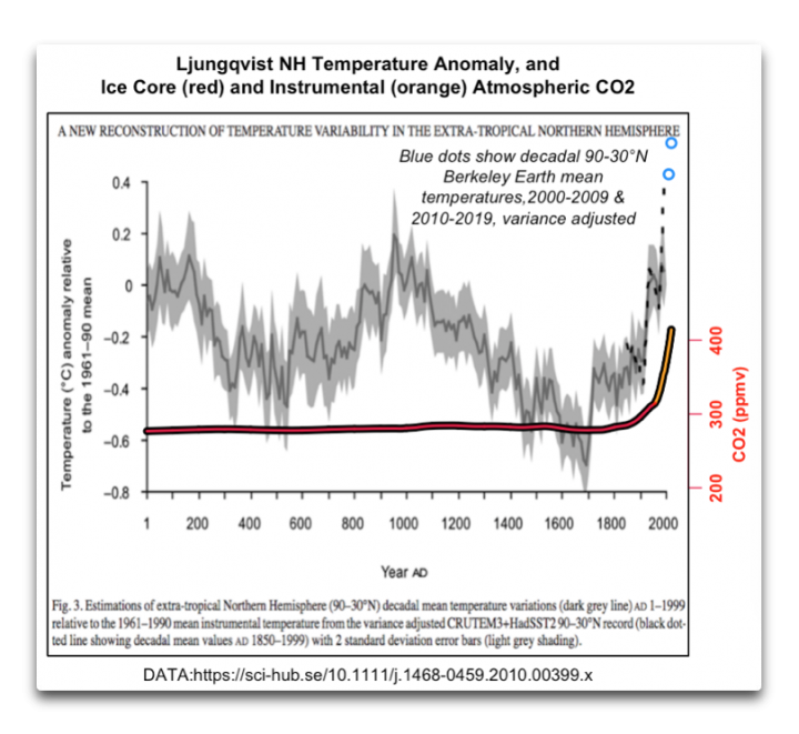
Figure 1. 2,000 years of temperatures in the land areas from 30°N to the North Pole, overlaid with ice core and instrumental CO2 data. Data source: A New Reconstruction Of Temperature Variability In The Extra-Tropical Northern Hemisphere During The Last Two Millennia
However, some folks have been saying things like “Yeah, but that’s not global temperature, it’s just northern hemisphere extratropical temperature”. I hear the same thing whenever someone points out the Medieval Warm Period that peaked around the year 1000 AD. And they’re correct, the Ljungqvist data is just northern hemisphere. Here are the locations of the proxies he used:
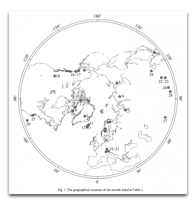
Figure 2. Location of all of the proxies used by Ljungqvist to make his 2000-year temperature reconstruction. SOURCE: Op. Cit.
So I thought I’d look to see just how closely related the temperatures in various parts of the globe actually are. For this, I used decadal averages of the Berkeley Earth gridded temperature data, file name “Land_and_Ocean_LatLong1.nc”. I chose decadal averages because that is the time interval of the Ljungqvist data. Here is a graph showing how well various regions of the globe track each other.
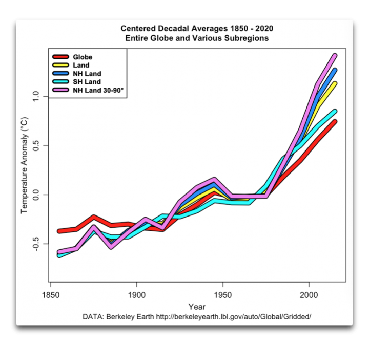
Figure 3. Centered decadal average temperatures for the entire globe (red) as well as for various sub-regions of the globe.
As you can see, other than the slope, these all are in extremely good agreement with each other, with correlations as follows:
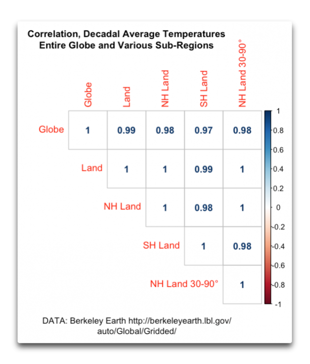
Figure 4. Correlations between the decadal average global temperatures and the decadal average global temperatures of various subregions. A correlation of “1” means that they move identically in lockstep. Note the excellent correlation of the extratropical northern hemisphere with the entire globe, 0.98.
This extremely good correlation is more visible in a graph like Figure 3 above if we simply adjust the slopes. Figure 5 shows that result.
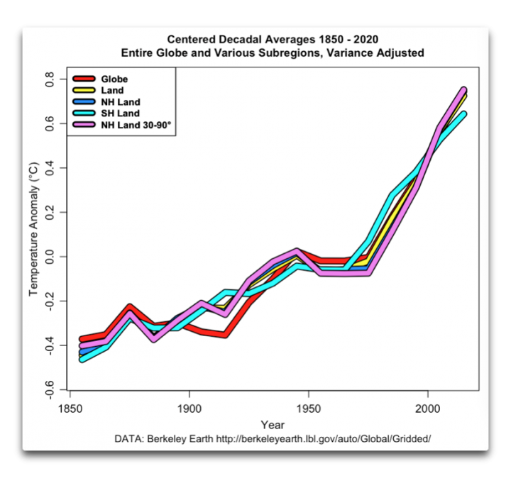
Figure 5. As in Figure 3, but variance adjusted so that the slopes match
Conclusions? Well, in US elections they used to say “As Maine goes, so goes the nation”. Here, we can say “As the northern hemisphere land 30°N-90°N goes, so goes the globe”.
Simply put, no major part of the globe wanders too far from the global average. And this is particularly true of large land subregions compared to global land temperatures, which is important since the land is where we live.
And this means that since per Ljungqvist the NH 30°N-90°N temperatures peaked in the year 1000 and bottomed out in the year 1700, this would be true for the globe as well.
As I mentioned in my last post, my gorgeous ex-fiancée and I will be wandering around Northern Florida for three weeks starting on Tuesday June 29th, and leaving the kids (our daughter, son-in-law, and 23-month old grandaughter who all live with us full-time) here to enjoy the house without the wrinklies.
So again, if you live in the northern Floridian part of the planet and would like to meet up, drop me a message on the open thread on my blog. Just include in the name of your town, no need to put in your phone or email. I’ll email you if we end up going there. No guarantees, but it’s always fun to talk to WUWT readers in person. I’ll likely be posting periodic updates on our trip on my blog, Skating Under The Ice, for those who are interested.
Best of this wondrous planet to all,
w.
“….started about the year 1700….”
interestingly the present day glass capillary thermometer was invented in 1714. And wasn’t accurate over a long term because the glass of the day slightly dissolved in mercury.
The 1690s were the coldest decade in the CET and probably the world. The Maunder Minimum lasted from about 1645 to 1715. But it also included the coldest winter, ie 1708-09.
There was another Great Frost in 1740-41, with associated famine. This ended the long, strong early 18th century warming cycle coming out of the MM.
Yep, History , the subject that is forgotten in schools
Forgotten or revised, or even fabricated.
As George says, although I would use the word corrupted to indicate the evil it represents.
As Maine goes …. and As California goes, so goes the nation for a lot of stuff, and regulating methane in new construction and other insanities will no doubt affect a lot of people in the near future. OK. That was off topic.
One day of hot weather in one city and we are told it is climate change, but, the Ljungqvist data is just weather.🤔
Who’s saying the Ljungqvist data us just weather? No one is saying that.
Thank you for a nice post! You are quite correct in pointing out that these warming events were in fact global. This has also ben documented by Yair Rosenthal(2013) evaluating proxies for OHC in the Pacific.. from the abstract: “Observed increases in ocean heat content (OHC) and temperature are robust indicators of global warming during the past several decades. We used high-resolution proxy records from sediment cores to extend these observations in the Pacific 10,000 years beyond the instrumental record. We show that water masses linked to North Pacific and Antarctic intermediate waters were warmer by 2.1 ± 0.4°C and 1.5 ± 0.4°C, respectively, during the middle Holocene Thermal Maximum than over the past century. Both water masses were ~0.9°C warmer during the Medieval Warm period than during the Little Ice Age and ~0.65° warmer than in recent decades. ”
REPORT Science 01 Nov 2013:
Pacific Ocean Heat Content During the Past 10,000 Years
Something does not seem right in figure 3 starting about 1975. I have no doubt that WE has correctly graphed BEST; the problem probably lies with BEST. It is not mathematically possible that the global result is appreciably lower than each and every of its constituent parts. And that divergence grows as today is approached.
Rud, the reason for the difference is simple—the ocean. I left it off because it isn’t really relevant to the question of land temperatures.
Best regards as always,
w.
My bad. I assumed Global was just land global. Duh!
It would however, be very interesting to see the ocean temperatures plotted too along with the rest just to illustrate how little they must be warming compared to the land areas.
Yes, I’d noted the same thing as Rud and was going to post to ask if you forgotten to point out this also included SST, since I’d guessed that was what was going on.
In fact BEST was always a land only analysis, at some stage they grafted in someone else’s SST so they could be “global” players.
It’s a great shame Muller did not stick to his original engagement and keep the skeptic players like Watts and Curry on board instead of going back on his word. It could have been a game changing unifying move.
Question: Isn’t the “land” temp primarily the air temp 1 meter above the surface while the “Sea” temp (SST) is not the air temp 1 meter above the sea surface?
We know that it’s irrational to claim the entire rise in the industrial age is man’ fault. The only valid hypothesis would only look at temperature above the ~1000 A.D peak. The fact that “97%” don’t do this tells you everything you need to know.
How is that rational? It assumes that the peak at 1000 AD is as high as natural warming can achieve. (Even though we know that the Roman warm period was warmer than the Medieval). And we also know that it was natural factors alone that resulted in the depths of the Little Ice Age.
You could have warming above the MWP that is still all-natural. Or you could have natural factors that would result in cooling if it were not for anthropogenic factors preventing cooling.
Your recommendation makes no sense at all. The only way to attribute temperature change to natural or anthropogenic causes is to understand the physical mechanisms. (So-called forcings).
Rich, if you were more familiar with our freind Zoe, you would not be so naive as to expect a rational statement. Just trust me, you do not want to spend too much time trying to explain anything to her.
Ha ha! Alas I have had a number of “friendly discussions” with the contrarian Zoe.
This was just my way of blowing her a kiss.
This coming from people who believe there’s a handful of beam-splitting layers in the sky.
Not only does Zoe have no idea what she’s saying, but she has no idea what other people are saying either.
Eemian. Much warmer.
Rich Davis
“Reply to
Zoe Phin
June 27, 2021 1:39 pm
How is that rational? It assumes that the peak at 1000 AD is as high as natural warming can achieve. ”
I see it better than comparing it to coldest earth been in about 8000 years- which was the Little Ice Age {which alarmist are frantic to erase from history].
Only thing about MWP is it peak for short period and cooled- I don’t think we start cooling that fast. So in that comparison one might imagine higher CO2 maintains the warmer temperatures, which I think is false.
Replacing one wrong answer with a wrong answer more to our liking?
How about putting 10% of the money swirling down the Climastrology toilet toward research into understanding the physical processes that control natural climate change?
I repeat myself, but the only way to ascribe natural or anthropogenic causes for climate change is to understand the physical processes involved.
Can we explain the Holocene Climate Optimum, and the Egyptian, Minoan, Roman, and Medieval Warm Periods? Then can we explain the Modern Warm Period in light of those five warm periods? What caused those natural oscillations? Why, in light of uniformitarian principles would we expect a sudden termination of those causes?
The null hypothesis should be that the Modern Warm Period would be caused by the same factors as the prior five warm periods. But until we explain what those causes really are, all we have is “nobody knows”.
Rich, the point is to give your opponents the chance to take the first step. They can’t even do that. Of course we can go back farther.
To use a financial markets analogy, i’s not “technical” analysis, it’s fundamental analysis that is needed here.
Good post. More confirmation that the MWP was global.
But the real question is… would Griff prefer living in 1700 to 1775 when CO2 was so benign, or this terrible time of over-carbon 1950-2025?
Griff?
Berkeley uses 1950-1980 as base for normals. There was no global data until 1979.
Berkeley has like 90% coverage (mostly interpolated) in 1940. It then averages only those available grid cells, and somehow calls this whole exercise global.
Would you please provide more detail about what you mean by “simply adjust the slopes”? Exactly what did you do to accomplish that, and why? Thanks…
Easy. If you ignore the fact that the NH Land warmed about 50% faster than the globe, the two metrics are identical.
In the HADCRUT data, trend in NH Land = 0.87C/century, Globe=0.53C/century.
https://www.woodfortrees.org/plot/hadcrut4gl/mean:120/plot/crutem4vnh/mean:120/plot/hadcrut4gl/trend/plot/crutem4vnh/trend
No idea what your point is here, John. In warming times, the land warms more rapidly than the ocean. In cooling times, the land cools more rapidly than the ocean … and?
My point was that although as you show, the slopes are different, the changes in the slopes occur at the same time, and differ only in value. For example, each of the changes from warming to cooling in both of your datasets occurs simultaneously in each dataset.
And thus, the same is almost certainly true about the changes from warming to cooling and vice versa in the Ljundqvist dataset being reflected in a corresponding change in global temperature.
w.
I used linear regression, which matches the variance of the two datasets. I did it to show that although the slopes of the trend are different, the changes in slope occur in tandem.
And this means, for example, that although the Ljundqvist data only shows the NH extratropical temperature bottoming out in 1700, it is clear that the entire world would bottom out at the same time.
w.
All data in climate science is “adjusted.”
Yes, Berkeley Earth is a bogus Hockey Stick. It doesn’t reflect the actual temperatures of the Earth in the early Twentieth Century.
Willis writes: Simply put, no major part of the globe wanders too far from the global average.”
What that says to me is we don’t need no stinkin’ bogus Hockey Sticks to measure the global temperatures. All we need are the regional surface temperature charts to find the global temperature profile.
All the unmodified regional surface temperature charts from around the world have the same temperature profile where they all show temperatures were just as warm in the Early Twintieth Century as they are today, which means the Earth is not experiencing unprecedented warming as the alarmists claime, and CO2 is a small, insignificant factor.
All the regional surface temperature charts have the same temperature profile as the U.S. regional chart which shows the 1930’s to be just as warm as today:
Hansen 1999:
So the actual temperature readings from around the world put the lie to the bogus, bastardized, computer-generated, fraudulent Hockey Stick charts of the world.
The real temperature profile of the globe is a benign one in which CO2 is a minor player. And Willis shows that regions of the Earth correlate, so we should dump the computer-generatied science fiction and go with the actual temperature readings for our global temperature profile, and we can forget about trying to reign in CO2. It’s unnecessary.
All data is adjusted, however some do their adjustments behind closed doors.
Of those who permit others to view their adjustments, some can be justified, some can’t. Most warmistas fall in the first category.
UAH is an example of a dataset in which adjustments are done behind closed doors.
GISS is an example of a dataset that is transparent. You can download their source code here and run it on your own machine.
If you find an adjustment GISS is making that you don’t feel is justified let us know which code file the adjustment is in and we can take a look together.
Dadburnit, Willis, that Ljungqvist chart up top looks almost like Mikey Mann’s hockey stick chart!! 🙂
Looks like Marcott’s also
Yes, the CO2 line looks similar — to Mann’s temperature line! Maybe that’s where he got the idea.
“Maybe that’s where he got the idea.”
Yeah, baby! He saw his goal and he matched it.
Now all we need to do is show where the CO2 came from in 1700 to accomplish the warming. It can’t be additional energy from the sun, because TSI doesn’t vary enough as we are always told.
Since CO2 is in fact the thermostat that controls global warming, according to modern climate science, it shouldn’t be too hard to locate the source. Of course, fossil fuels did not exist then and we are also told volcanoes are not important sources. So it must come from some other source, unless the physics decided to change between 1700 and now.
CO2 is a thermostat; not the thermostat. CO2 is likely not a significant factor in the 1650-1750 period since it didn’t change all that much. Aerosol and solar radiation likely dominated over CO2 as significant EEI influencers. Ocean circulation change the transport and distribution of heat in the climate system so they have to be considered as well in the context sub-global warming/cooling trends. In fact, the AMOC remains a viable candidate to explain the observations Lamb first noticed in the NH and especially in and around the North Atlantic where the MWP and LIA were most acute. Remember, there are a lot of factors that can modulate hemisphere and global temperatures. These factors ebb and flow so you cannot assume that a set factors that dominated in the past will be the same as those dominating today.
Wrong terminology. CO2 concentration is a factor, not a thermostat. A thermostat is a mechanism for maintaining a static temperature by turning on heating when temperature falls below a setpoint or turning on cooling when temperature exceeds a setpoint, or both. CO2 is certainly not that.
Alarmists have a doctrine of faith that CO2 is the master control knob which determines temperature. This is what drives them to desperately try to disprove that there have been millennial-scale warm periods and/or to claim that the warming was regional and offset by cooling in another region where conveniently there is no historical record one way or the other. Willis shows evidence that temperature in all regions move in concert, arguing that natural warm periods were global. This blasphemy offends the religious sensibilities of the alarmists.
Proxy data doesn’t show the substantial changes in CO2 that could explain a warming or cooling period. Therefore since their motivation is to prove that modern period increases in CO2 are the sole cause of warming, alarmists must deny the evidence of any past temperature change. They deny any significant warming and/or claim that volcanic eruptions which modern evidence shows to have only a marginal short-term effect, explain any cooling periods.
Settlements in Greenland, tree stumps revealed by receding glaciers, frost fairs on the Thames are all denied in order to sustain their article of faith.
Natural climate change deniers abound.
Can’t speak for ‘alarmists’, but this is not my understanding of the current climate science consensus (as expresed by the IPCC). CO2 is considered to be the current main determining factor. It is not considered to be the only factor determining global temperatures over the longer term.
Nonsense, any time you speak, you speak for alarmists, TFN.
Mann and others have long labored to “disappear” the MWP and falsify the temperature record to keep it consistent with a world where rising CO2 causes rising temperatures—without any examples of warming or cooling that is not the result of CO2 change. Volcanic and aerosol pollution deus ex machina explanations need to be employed since some aspects of history are undeniable.
Temperature started rising 250 years before CO2 really started to change. So what caused that and why is that cause no longer active?
CO2 has a minor warming effect, maybe 1.7K per CO2 doubling. This is not denied on the climate realist side. We are not climate change deniers like you and Nick.
1.7K for equilibrium climate sensitivity is inside the IPCC AR5 likely range (1.5-4.5K with medium confidence). I guess that makes them climate realists too.
Yes, many of the real scientists in group 1 are climate realists. It’s the extremist politicians and activists who drive the >4.5 ECS estimates.
Ummm … no. Mostly it’s climate models driving the high estimates, particularly the CMIP6 models.

w.
I think one thing you and I would agree on is that the higher CMIP6 ECS should be considered with a healthy dose of skepticism. From what I hear the newer cloud microphysics scheme may be the cause of the higher ECS. The schemes work well for operational numerical weather prediction so I can understand the impetus for porting them to climate models. But when those schemes are ported to paleoclimate models they seem to reduce the skill of the model in explaining things like the glacial cycles. I think that is a clue that these newer schemes may have a long term time dependent bias that is not evident in the time scales involved with operational weather forecasting. We’ll see how this plays out in the coming years.
Deducing ECS from these models is a crock.
And who gets to decide what constitutes “equilibrium”?
Nah. They chronically miss cold air beyond a week or so. Long-term forecasts are pitiful — always too warm.
“work well” is objectively defined as an anomaly correlation coefficient >= 0.6. NWP maintains >= 0.6 for 500mb heights out to about 8 days now. The useful skill range has been slowing increasing with each passing decade as the cloud microphysics, other physical schemes, and the numerical cores in general improve.
https://www.emc.ncep.noaa.gov/gmb/STATS_vsdb/
Well yeah, climate models created by politically-motivated pseudoscientists to gather grant money. But there are still some non-alarmists involved with the IPCC don’t you think?
Thanks, Rich. Perhaps you could name say a half-dozen of them, instead of speculating?
w.
OK, I will stand corrected if that’s your considered opinion. Back in the old days there were some realists in group 1. Maybe they have been fully purged.
Willis: Any change in the regional temp data related to the 1815 Tambora volcanic explosion that caused a “year without a summer” in 1816 and much hardship in Europe and North America Atlantic Coast?
You can discern a confidence interval from a tri-modal distribution?
Show your work, please.
Just barely, at the low end.
However it provides yet more data to show that the high end, 4.5K is utter nonsense.
Regardless of what the consensus of climate “scientists” is, there isn’t a shred of data to support the belief that CO2 is the current main determining factor in determining climate.
You’re pulling our legs, right?
“consensus” and “IPCC” and “considered”?
Next you’re gonna quote Al Gore and Gretha Thurnberg, and use that to ‘prove’ Michael Mann is a direct decendant of Mother Mary?
How old are you, child? Time to gather some logical understanding, instead of just memorising enough “facts” to pass the test.
I shall not ask who you think is setting the test you seem to be swotting for…
There are two IPCC’s. The first is the actual data, and even after filtering to make sure that known skeptics are not permitted in, it still doesn’t support the alarmist mantra.
The second is the Summary for Policy Makers, which in many cases was written even before the individual chapters were finished and bears little relationship to the science developed in the chapters themselves.
No argument here on preferring the term factor over thermostat. And I agree that CO2 does not have the ability to turn on/off it’s radiative effect in a binary manner like a thermostat. Don’t hear what I didn’t say though. I didn’t say that CO2 has no radiative effect. It does. And it’s effect changes in proportion to the amount of it in the atmosphere.
Willis presents evidence that global and some regional temperatures are correlated from 1850 to present. It is evidence that I do not reject.
Others present evidence that global and some regional temperatures are not always correlated. It is evidence that I do not reject.
I think everyone (alarmists, contrarians, and mainstream alike) accept that there were substantial warming/cooling periods in the past both regional and global in scale.
Paleoclimate records DO show that substantial changes in CO2 are a modulating factor in many warming/cooling eras. The PETM, other ETMx events, glacial cycles, the faint young Sun problem, and many other events and topics cannot be explained without invoking CO2 to some extent. Don’t hear what I didn’t say. I didn’t say that CO2 is the only factor that modulates the climate or that it is the only thing that dominates in every climatic change episode.
Anecdotes that Greenland was habitable is consistent with Lamb’s original research, recent research, and the AMOC hypothesis.
I think everyone (alarmists, contrarians, and mainstream alike) accept that there natural factors that modulate the climate system.
“Paleoclimate records DO show that substantial changes in CO2 are a modulating factor in many warming/cooling eras.”
Like what?
The PETM, other ETMx events, the glacial cycles, and the faint young Sun problem were the examples I gave.
The PETM effect is assigned using climate models. Undemonstrated.
In the glacial cycles, CO2 trails temperature. No modulating factor there.
In the earliest Paleocene (post Hadean), the atmosphere was ~60 bars of CO2 and 0.8 of nitrogen. Hardly an apt comparison with CO2 and the modern climate.
When multicellular animals evolved up, about 700 million years ago, the sun was well on its way to modern brightness.
CO2 both leads and lags temperature. It leads when it is the catalyzing agent for the temperature change and it lags when another catalyzing agent is in play. But in both cases temperature modulates CO2 and CO2 modulates temperature. And although the blogosphere likes to promulgate the myth that CO2 only ever lags using the Quaternary Period glacial cycles the reality is far more nuanced (see Shakun 2012). But even if it did wholly lag the temperature (it may not have) the glacial cycles still cannot be explain without invoking CO2’s modulating effect on the temperature.
The solar forcing 700 million years ago was about -14 W/m2 (see Gough 1981). CO2 would have had to have been 6000 ppm with +14 W/m2 of forcing just to offset the lower solar output.
I’m not sure what the challenge is with the PETM. Can you post a link to a publication coming to a significantly different conclusion than that of a large carbon release followed by a large temperature increase?
Okay, I’ll bite:
Now, please explain in detail, how exactly do you (or your climastrologist seers) decide when CO2 was the catalyst, and when it was something else.
Also, define that ” ..another catalyzing agent..”
Ad hominem: I bet you ‘win’ a lot of arguments by saying: “oh, that’s just whataboutism”.
By “another catalyzing agent” I mean anything that can perturb the EEI directly or indirectly other than CO2. Milankovitch cycles, grand solar cycles, and volcanism would be obvious examples here.
CO2 is a catalyzing agent for a temperature change when no other agent acts first to perturb the EEI. This occurs when CO2 is released independent of the temperature like would be the case with volcanism or extraction of carbon from the fossil reservoir.
Give evidence of it being catalyst, you can’t because other then the climate models there is none.
Somehow I don’t think the time resolution of the data you’re looking at really allows you to determine whether a CO2 increase came before or after a temperature increase, especially from multi-million years ago.
Shakun 2012 is a crock. See also Liu, et al., 2018 who show that change in CO2 was a feedback, not a driver, of the last deglaciation.
The notion that “CO2 modulates temperature” is an artifact of physically meaningless climate modeling.
With no adequate physical theory of climate, no one can say how the climate was clement during the fainter sun. You’re just imposing your stock deus ex machina did it! explanation. False precision as a cover for ignorance.
Fake diversion on PETM. The question is not about gas releases or temperature change. The question is whether CO2 drove temperature. Climate models can reveal nothing about it.
That Liu publication is good. It’s already in my collection. It’s definitely falls more in line with the consensus view that Milankovitch cycles were the primary trigger the initial temperature change and it does so using data provided by Shakun. So if you think Shakun is a crock then you’ll probably think Liu is a crock as well. Anyway, the publication discusses the Shakun 2012 conclusion and reasons for disagreement which I do not reject. Note that Liu definitely agrees with the consensus that CO2 modulates the temperature and that there were periods in Earth’s past where it was the initial trigger. He just doesn’t think the evidence supports it for the last deglaciation which I happen to agree with. Definitely read his other publications though. He definitely sides with the mainstream view that CO2 is a significant contributing factor to current warming era.
The PETM is far from a diversion. It is an event in Earth’s past where there was a large increase in both temperature and airborn CO2. That makes it spot on relevant to the question of the lead-lag behavior of the two. However inconvenient it may be it is still one example of where CO2 was the initial trigger for the temperature change.
“a large increase in both temperature and airborn CO2. That makes it spot on relevant…”
You’re arguing correlation = causation; a very naive mistake.
Liu, et al., 2018 say this in conclusion: “Overall, the results of breakpoint analyses on global and hemispheric scales show a clear DCI lead over aCO2 at the early stage of the deglacial warming, suggesting that aCO2 is an internal feedback in Earth’s climate system rather than an initial trigger. (my underline)”
where DCI is their “deglacial climate index.” Liu, et al.’s conclusion opposes your claim.
Liu, et al., appear to have accepted Shakun 2012 at face value; now known to be a big mistake.
Kiehl, 2007 showed that climate models vary by 2-3 fold in their respective ECS and all still manage to reproduce the 20th century trend in air temperature through the magic of off-setting errors. And yet he “agrees with the consensus that CO2 modulates the temperature...” Such agreement is likely a sine qua non of publication. It means nothing.
“Propagation …” demonstrates that there is zero scientific evidence that CO2 modulates air temperature.
“Negligence …” demonstrates that the entire consensus position is artful pseudoscience; a subjectivist narrative decorated with mathematics.
Liu et al. 2018 concludes that DCI leads CO2. This is consistent with my personal position that CO2 was not the initial trigger or catalyzing agent for the glacial cycles.
Liu et al. 2018 does NOT conclude that CO2 always follows temperature. In fact, other Liu publications make it clear that he accepts that CO2 sometimes leads the temperature.
Liu et al. 2018 does not accept Shakun et al 2012’s interpretation at face value. In fact, they present their own interpretation. That is the whole point. But they still use the Shakun database.
It is not possible from these two publication alone to adjudicate between the Liu and Shakun interpretations.
Both Shakun and Liu accepts that CO2 modulates temperature and that temperature modulates CO2.
I’m not saying that correlation = causation. I’m saying that the PETM is an event in which both CO2 and temperature increased. That alone, regardless of which was driving which, is enough to make it relevant to lead-lag discussions. That necessarily means it is the opposite of a diversion. The fact that CO2 was the trigger for the temperature increase for this event is not based on correlation. It is based on the causative mechanism that was first identified in the 1800’s and verified time and time again ad-nauseum since. The PETM is a test of the hypothesis “CO2 only ever lags the temperature”. It turns out that this hypothesis is false as evidenced by the PETM.
“That alone, regardless of which was driving which, is enough to make it relevant to lead-lag discussions.”
Tendentious. You have no idea whether either was driving the other. Neither does anyone else.
Your demurral of CO2 as trigger is gainsaid by your own prior text, namely, that the “Liu publication is good,” and it “agrees with the consensus that CO2 modulates the temperature and that there were periods in Earth’s past where it was the initial trigger.”
Clearly, by logical adherence you agree with the position that CO2 has been a trigger.
No “causative mechanism that was first identified in the 1800’s” because no physical theory of climate existed in the 1800s. Only the idea of radiative forcing by CO2 was first developed in the 1800s. A causative physical theory is not in hand today, either.
Furthermore, it is fully demonstrated that there is no evidence that CO2 radiative forcing can play any role in air temperature. The only relevant ad nauseam is the willful disregard of that demonstration by CO2 cultists.
The 10 My timestep of PETM CO2 and air temperature disallows any resolution of a lag, mooting your entire argument along that line.
It doesn’t matter which is driving which. Any event in which CO2 and temperature are correlated is relevant to lead-lag discussions. The PETM is not a diversion. It is spot on relevant to what we are discussing.
Yes. I absolutely agree that CO2 has catalyzed temperature changes. Liu agrees. Shakun agrees. Pretty much everyone including even the most vocal skeptics universally agree.
We don’t need a comprehensive physical theory of the climate system to know that certain gas species impede the transmission of radiant energy. That mechanism was decisively demonstrated in the 1800’s. This knowledge is used successfully in operational meteorology to detect water vapor in the atmosphere. It is also used in fields unrelated to weather or climate. It is not challenged or controversial in the slightest. Just because you reject the body evidence or are unfamiliar with it does not mean that the mechanism is nonexistent. BTW…the radiative forcing and radiative transfer schemes were pioneered by Gilbert Plass in the 1950’s; not the 1800’s.
One paper published by you and criticized here, here, and here with even “skeptics” challenging it does not constitute “fully demonstrated”. To my knowledge your research has not be replicated.
And I have no idea why you would post a link to that Gehler et al 2015 publication. That one is in my archive as well so I’m familiar with it. And note what the conclusion is: “Our results are consistent with previous estimates of PETM temperature change and suggest that not only CO2 but also massive release of seabed methane was the driver for CIE and PETM.”
“It doesn’t matter which is driving which.”
Yes, it does. T driving CO2 reflects standard solubility. No big deal. CO2 driving T is your be-all and end-all of global warming.
“Any event in which CO2 and temperature are correlated is relevant to lead-lag discussions”
No, it isn’t. For the reason noted above.
“Yes. I absolutely agree that CO2 has catalyzed temperature changes.”
With zero justification.
“We don’t need a comprehensive physical theory of the climate system to know that certain gas species impede the transmission of radiant energy.”
Irrelevant. Neither you nor anyone else knows how the climate responds to the K.E. CO2 injects into the atmosphere. You need a comprehensive physical theory to describe that. You’ve not got one. Neither has anyone else.
No AGW cultist seems to have the remotest notion of how science works.
“BTW…the radiative forcing and radiative transfer schemes were pioneered by Gilbert Plass in the 1950’s; not the 1800’s.”
Lightfoot & Mamer (2014) Calculation Of Atmospheric Radiative Forcing (Warming Effect) Of Carbon Dioxide At Any Concentration E&E 25 8, 1439-1454,
p. 1439: “In 1896, Arrhenius identified C02 as a greenhouse gas and postulated the relationship between concentration and warming effect (radiative forcing) was logarithmic.”
Oops.
You didn’t read my debate with Patrick Brown below his video, did you. Or maybe you did read it and didn’t understand it.
He’s a nice guy, and sincere, but showed no understanding of physical error analysis, or of the meaning of systematic error, or of calibration.
And like every climate modeler I’ve encountered, Pat Brown showed no understanding even of the difference between an uncertainty in temperature and a physical temperature.
I showed the poverty of Nick Stokes’ attack here.
And Ken Rice, Mr. ATTP, couldn’t figure out where the ±4 W/m^2 cloud forcing error came from, even though I spent 3 pages in the paper explaining that very point. His criticism is hopelessly inept.
“To my knowledge your research has not be replicated.”
Several people have done so. You could do so.
And I’ve replicated it right here. And with CMIP6 models. They’re useless, too.
If you understood “Propagation …” , you’d know it demonstrated the case that air temperature projections are physically meaningless.
“And note what the conclusion is” Consistent with physically meaningless modeling results.
I noticed you did not address this from Rich Davis, above:
“Temperature started rising 250 years before CO2 really started to change. So what caused that and why is that cause no longer active?”
His post was not meant for me. Though I suppose I can address it now. The leading hypothesis is a combination of a new solar grand cycle, reduced aerosol loading, and an increase in the AMOC. These factors are still active just in different proportions and generally with opposite signs. Since 1960 solar radiation has decline, aerosol loading has increased, and the AMOC has slowed down. This puts downward pressure on the NH temperature.
bdgwx posted: “The leading hypothesis is a combination of a new solar grand cycle, reduced aerosol loading, and an increase in the AMOC.”
Now that’s a real witch’s brew if I ever saw one.
There’s nothing magic about solar forcing, aerosol forcing, or the AMOC.
bdgwx posted “There’s nothing magic about solar forcing, aerosol forcing, or the AMOC.”
I never said there was. It was you that used the words “combination” and “and”, thereby tying all together.
“Noun 1. witch’s brew – a fearsome mixture . . . assortment, miscellanea, miscellany, mixed bag, motley, potpourri, salmagundi, smorgasbord, variety, mixture – a collection containing a variety of sorts of things . . .”
—source: https://www.thefreedictionary.com/witch%27s+brew
Aerosol forcing is the adjustable fudge that makes the rest fit.
Along with a liberal dose of hand-waving word salad.
That’s the rub. Nobody has any idea what kind of or how much aerosols were in the atmosphere decades ago, much less hundreds of years ago.
This provides the flexibility to adjust the aerosol mixture and concentration until your model produces the output you were looking for.
Translation: We don’t know, but we gotta come up with something to defend the notion that only CO2 is impacting temperatures now.
CO2 isn’t the only thing impacting temperatures now.
A meaningless statement. No one knows whether CO2 is impacting temperatures now. Or whether it ever did so.
Word-salad hand waving.
1700?
.
https://www.reference.com/history/invented-first-steam-engine-year-1c5f5b863560d363
..
https://www.18thcenturycommon.org/tags/coal/
Volume matters.
The increase at the time was on the orders of single parts per billion over many decades.
If those tiny increases in CO2 was enough to drive the temperature seen back then, than today’s increases in CO2 should have increased temperatures by 10’s of degrees.
” Of course, fossil fuels did not exist then . . . “
The intent here is clear enough, but the statement is still wrong.
Coal was used as a fuel in Britain since Roman times.
“And this means that since per Ljungqvist the NH 30°N-90°N temperatures peaked in the year 1000 and bottomed out in the year 1700, this would be true for the globe as well.”
The rise in the last century has been due to a global effect – increasing GHGs. There is no guarantee that would be true for those earlier temperature movements. The cause may have been local.
Nick, as shown in Figs. 3 & 5, the temperatures have gone up, flat, and down during the period, and those movements of the global temperature match those of the NH extratropical temperature with 0.98 correlation. If you think that’s due to CO2, you need professional help.
w.
Is the 0.98 correlation not for the 1850 to present period though? What is the figure from 0 to 1850? I think given what we now know about ocean circulations like the AMOC we need to eliminate it as a significant contributing factor to the NH temperature swings during this era before we assume the NH and SH swing in tandem especially considering research like that of Shakun et al. 2012 and others indicates the NH and SH have exhibited seesawing behavior in the past.
Willis,
In those figs, apart from a pause following 1950 due to aerosols, it is rising all the way. Not linearly, but the rise of CO2 wasn’t linear either.
But the trend was rising and so that is the null hypothesis. Rising.
Also it means anyone who believes all the warming is anthropogenic in nature is coming from a place of ignorance.
Using the Ljungqvist proxy data, the trend from 1660 – 1900 is 0.14°C / century, the trend from 1900 – 2000 is 0.38°C / century, with a standard error of ± 0.01°C / century.
The warming in the 20th century is significantly faster than the previous warming.
Bellman, the fastest warming in the Ljungqvist data is the thirty years after the bottom in the LIA when it warmed 0.36°C in less than a third of a century. There is nothing in the post-industrial era that even comes close to this.
w.
Let’s assume it is a fourth of century. That is 1.4C/century. The instrument record from 1979 has a trend of about 1.8C/century.
No difference between the two.
I think you are reinforcing my point. It’s claimed that there was a warming trend over the last 300 years, in reality most of the pre-20th century warming happened in just those 3 decades, and starting in an exceptionally cold decade. After this temperatures hardly changed until the early 20th century, a 150 year pause.
It’s difficult to argue that the 20th century warming was a continuation of a warming trend that ended in 1740.
The significant rise in CO2 didn’t start until around 1950. Why don’t you use some realistic dates?
“Using the Ljungqvist proxy data, the trend from 1660 – 1900 is 0.14°C / century, the trend from 1900 – 2000 is 0.38°C / century, with a standard error of ± 0.01°C / century.”
Yes, as MarkW said, the date ranges to compare are 1660 – 1955 and 1955 – Current.
Why would you choose 1900?
I chose 1900 because the discussion I was responding to was talking about warming in the 20th century.
But I’d be dubious about basing any shorter test on the this data given it doesn’t reflect 20th century instrumental records very well, and anything looking at just the last few decades won’t have much significance.
I’m also not really sure why you think 1955 is the magic place to start. CO2 was rising throughout the 20th century and temperatures mid-20th century were likely being effected by atmospheric pollution.
Still for the record
“Using the Ljungqvist proxy data, the trend from 1660 – 1950 is 0.16°C / century, the trend from 1950 – 2000 is 0.11°C / century, with a standard error of ± 0.21°C / century.”
Note, the large uncertainty given this is based on just 5 data points. Also note that whilst the trend since 1950 isn’t significantly different from the trend up to 1950, the actual temperatures are somewhat higher than expected.
For comparison CET gives a trend from 1660 – 1954 of 0.18°C / century. 1955 – 1999, 1.68°C / century.
(That’s using annual rather than decade data)
I thought the IPCC attributed from 1955 but in fact they attribute the anthropogenic warming influence of CO2 from 1950
From IPCC AR5 we have
So regarding
Again, the null hypothesis is rising. And attribution of CO2 is far from “all of it”
Belief that the warming since 1950 is mostly attributed to CO2 has come from the models and the models are not fit for purpose of climate projection except as a fit to their tuning. I dont expect you to believe or even understand that.
You probably dont even realise models played a key role because the whole attribution certainty has been lost in a relatively short history of AGW memes such as “we cant predict 10 yearly climate but we can predict 100 year climate” which is utter nonsense but put out there strategically IMO.
Nick knows better, I am not sure why he keeps up the BS. It’s one of the things that baffles me the most here.
If the global warming scam collapsed, Nick would have to find a new job.
The cause for the peak in year 1000 was what?
Well, it was likely the same cause as for year 200…the Roman warming period….and the one before that ….Egyptian Warming Period…and the one before that….and as for those interim cooling periods…the inverse? Really, if the warm-mongers cannot explain the past, including 1941 to 1980 cooling…then why do they have any credibility? And, not to mention why 1930s warm(hot) period has been doctored by NASA.
Why would all warming and cooling periods necessarily have to be caused by the same thing?
So, what are your suggestions? The fact that there have been cycles of climate for the last 8000 t0 10000 years suggests Nature will continue the cycles until it doesn’t. Another deep Ice Age is on the calendar in the next few thousand years if Nature repeats again. Don’t worry….the ultimate climate in the future is warm really warm….when the sun really starts running out of fuel and becomes a red giant.
My suggestion is that of mainstream climate science theory. That is that there are many factors that modulate the climate. These factors ebb and flow. No two periods of warming/cooling are caused by the same set of factors in exactly the same proportions. And certainty no one factor is always the dominant cause for all climatic change episodes.
Fair enough. I endorse that statement. And the effect of CO2 currently is modest and likely to be beneficial up to and including any practical level of emissions, given that empirical evidence shows that ECS is around 1.7K.
It could be 1.7K, but that is looking less likely by the decade. It could also be 3K or 4.5K. The most comprehensive research to date puts the 95% range at 2.3-4.7K. See Sherwood 2020 for details.
The fact that more and more politically-motivated “studies” and models that vastly overestimate actual temperatures is in your mind evidence that actual measurements won’t prove to be accurate?
The fact that ECS estimates have diverged in the 42 years since Charney gives you confidence somehow to weight models over empirical evidence?
Help me out here. I’m just an old fool denier.
If you know of a global mean temperature dataset which you trust we can use it to compare the others and see just how much they overestimate actual temperatures to relative to it. And if you can provide supporting evidence for using that selected dataset as a gold standard then we be able to consider the overestimation in error especially if this gold standard dataset can be reviewed for significant mistakes and replicated.
The fact that the confidence intervals of ECS estimates have not improved significantly is unfortunate. Though that may finally be changing (see Sherwood 2020). Anyway, the biggest problem is on the right hand side tail from the mean/median. It’s easy to constrain the left hand side tail using observations. The right hand side…not so much. The spread on the right hand side and why there is such a long tail is the feedbacks and tipping points.
FWIW I don’t think you’re a fool or denier.
There are no confidence intervals for ECS, the distribution is garbage.
I agree that there are many factors that influence climate. There is no evidece that CO2 is one of those factors.
To be fair, there is at least theoretical evidence based on lab experiments that, being a gas that absorbs IR in certain bands, it must be a factor in reducing the rate of radiative cooling. Whether it’s a major factor that dominates over other factors is where there is not a shred of evidence. The theory of positive feedbacks far exceeding the direct effect is in my view already falsified by 40+ years of empirical evidence.
Sorry to be so late here. Reducing the rate of cooling doesn’t equate to an increase in maximum temps. Daytime temps do not appear to be driven by minimum nighttime temps. The sun drives maximum temps, not minimum nighttime temps.
That being the case, mid-range temps going up are basically meaningless insofar as trying to use them to claim the their increase means we are all going to die.
Tim,
Your point that most warming occurs at night (and btw therefore most significantly during winter and outside the tropics) is certainly true.
Radiation doesn’t know about day or night, though. It follows the Stefan-Boltzmann law 24/7. The surface radiates more when it is hotter (sun is shining) than when it is cooler (at night). The upwelling IR is still inhibited during the day. Convection usually dominates cooling during the day, so it’s a complex question, but Tmax should theoretically still increase somewhat when there is more GHG in the atmosphere. The right question is “Is it significant?”, and the answer is no.
God doesn’t play dice with the universe and you have just described a dice game.
I described no such thing.. What I did was communicate the conclusion of Sherwood 2020. I encourage to you read the publication. If you have questions I’ll do my best to answer them.
You basically outlined sceptic’s position. Until you can disprove that other factors are NOT at work, then you can not rule them out! That still leaves CO2 as a minor player and spending trillions upon trillions on a whim is unforgivable.
That same bar of skepticism cuts both ways. All possibilities including CO2 remain candidates as significant contributing factors until falsified. It turns out that for the current warming era (at least since 1960) we can eliminate the Sun since solar radiation is has declined, aerosols since the loading has increased substantially, Milankovitch cycles since they work on really long scales far longer than the 100 or even 10 year scale embodied by this round of warming, and the AMOC since it is declining to provide a few examples. One other powerful observation that any hypothesis must survive is the cooling stratosphere. That eliminates a vast array of possibilities right there.
Hand-waving.
Until you can demonstrate what caused the earlier warm periods, you can’t demonstrate that the same forces (whatever they are) are not causing the current warm period.
Exactly
Nah. Science does not require 100% perfect understanding to be able to provide useful explanations and predictions of past, present, and future events. We don’t have to explain every event to be able to explain some events and to predict future events with reasonable confidence. This is true for all disciplines of science. It’s one of the things makes science…science. But steering this thread back on point we can eliminate forces for the current warm period. We can eliminate solar radiation since it is declining, we can eliminate aerosols since they are increasing, and we can eliminate the AMOC since it is declining. So yes, we can eliminate some possibilities for the warming today even though our understanding of the paleoclimate era is imperfect.
What warming are you seeing? Warmer minimum temps? Warmer maximum temps? Both?
Both. But the warming is most apparent with minimum temps.
The warming and cooling periods match up very well with Atlantic Ocean salinity changes. They might very well be all caused by the same thing.
https://www.nature.com/articles/s41467-018-02846-4/figures/2
The salinity variability could be due to the MOC bringing different levels to the surface starting way back as melt pulses. That would make them aftereffects of Milankovitch cycles.
In recent decades this effect could also be enhanced by microplastics. Both will lead to reduced evaporation driving warming. Difficult to assess since increased CO2 likely drives more evaporation instead of warming.
That publication says anthropogenically caused warming is one factor responsible for changing ocean circulations that contribute salinity changes. Milankovitch cycles are not suggested as factor in the publication. So the “same thing” you seek is AGW at least according to the publication you linked to here.
Would that not imply that all or almost all local causes were correlated in a warming direction and that they all stopped working 100 years ago so fossil fuels could take over?
No, nothing stopped 100 years ago. AGW is added to all the other sources of variation. But it’s big.
Now all you gotta do is find some empirical evidence and prove it. Should be easy.
There are published graphs of CO2 and temp going back millions of years…how accurate?….don’t ask me but there is no correlation on those graphs…in fact, it is the opposite of correlation…almost.
It is the same with the Sun. On time scales of millions of years the solar factor has no correlation with temperature. In fact, it is the opposite of correlation. This is the essence of the faint young Sun problem. But, a composite of the solar forcing and the CO2 forcing together provides a far better correlation than either of them alone. It is a testament to the fact that no one thing can adequately explain global mean temperatures on this time scale or any time scale really. All factors must be considered.
If the AGW warming is on top of the already happening warming, then there doesn’t seem to be much room for CO2 to have caused any warming.
Since the increase in the rate at which temperatures have increased over that period is small to non-existent.
If CO2 is big, and being added to whatever was going on before, then we should see a huge increase in the rate of warming once CO2 levels started rising.
No such rise is evident in the record.
Now there’s a quantitative analysis! “It’s big”
So you are arguing that whatever caused the warming since 1700, conveniently stopped as soon as CO2 started rising.
Really?
Care to prove that conjecture?
No. He is saying that all factors matter. In other words GHGs and aerosols have the exact same effect in the exact same proportions regardless of whether those elements were naturally modulated or anthropogenically modulated.
But the models that “show” the warming start out flat. That’s what the control runs show. No warming. So your statement of factors excludes natural warming.
Mark, since CO2 has been increasing at an accelerating pace and temperatures have not then their “big” most be happening while natural cycle are in a cooling phase otherwise natural temperature increase plus “big” CO2 affect should be causing a dramatic increase in temperature. So for Nick and Bdgwhatever to acknowledge that there is a natural increasing cycle invalidates their own CO2 “big” affect BS.
Again Nick knows it’s all BS there is something else going on with him, it’s only a matter of time until he admits it.
If that is true, then you are defeating the very Global Average Temperature you rely on. You are postulating that CO2 is not a well-mixed gas that is THE main factor in determining temperature. The conclusion is that “local” conditions do not determine GAT.
If the sea temperatures are held constant, and you play with the land temperatures, you will quickly see that northern hemisphere land temperature changes dominate the resulting ‘average temperatures’.
Simply put, there is much more land north of the equator than there is south of the equator. Sea temperatures aren’t fixed, but they vary much less than land temperatures do. This means that the northern hemisphere land temperatures are going to drive the resulting averages.
I still don’t know what averaging temperatures really means. What does it mean to average desert temperature with mountain temperatures above one kilometer above sea level? (beware of overlap). What does it mean to average sea temperatures with land temperatures?
I don’t know, but I do know that the resulting averages can say things that mean absolutely nothing. These averages are like that song about war. What are they good for? Say it again! Keep saying it until people start to see.
You are correct about averaging actual temperatures. South Florida isn’t Chicago. In climatology, the problem is avoided by globally averaging only the anomalies computed from from some actual average baseline (say 1980-2000) for each station separately.
You haven’t solved the what does it mean question. It applies to time series too.
But now that you bring it up, there is much more hidden. Chicago is a lot smaller than south Florida. Miami might be a better comparison, but there are going to be large variations in the spread of measuring devices, so the readings of sparser devices will have greater contributions to any average weighted by area.
And what happens when we add or take away a measuring device to or from the everglades? How do we correct for somebody pointing out that such a device is poorly maintained, or has lost good siting? Or it has been moved? Once you start working in differences little things have big effects.
Frankly, I can drive around and see the temperature go up and down depending on my position. And I can watch local news show a map of these local variations based upon measuring stations they set up in viewers yards. Yet only the one at the airport counts?
What you are describing is a license to make up whatever they want with a nice gloss of ‘see all were doing to make it look real’ thrown on top to cover up what they are doing.
I have sat in rooms where experimenters were tearing each other apart over issues affecting and sometimes even flaws in their experiments. Some had clearly thought things through better than others, and it showed quite clearly. It really shows.
Introducing a phony calculation – “anomalies” – does not serve the “science” of climatology well as long as the presumed effect of a 2K increase in the anomaly changes the “climate” the same whether it results from a 4K change in Tmin with no change in Tmax or the inverse, or whether it occurs in a region with daily (Tmax- Tmin) <10K or >50K. “Climate” is not meaningfully measured by average temperature in any guise.
““Climate” is not meaningfully measured by average temperature in any guise.”
The problem is that the temps being used are not even “average” temperatures. They are mid-range temperatures. Since daily temps are a time varying series, resembling a sine wave, the average temperature is *not* the mid-range temp.
Absolute anomalies are not usually shown with a variance. The variance in absolute temperatures and anomalies are identical. What does that mean? It means the variance can be larger than the anomaly being used. Taking the square root of the variance to get Standard Deviation doesn’t help much. The GUM specifies that uncertainty can be reported with the SD. So you end up with an uncertainty interval that dwarfs the average anomaly.
Secondly, you can not simply average anomalies and claim that the variance has been reduced. Variances add when combining populations, i.e. station averages. The variance is never reduced.
“Variances add when combining populations, i.e. station averages. The variance is never reduced.”
As far as I can tell you are talking about the variance of the sample. But so what? Assuming you really mean Standard Deviation here, all you are saying is how far from the mean an individual measurement is likely to be.And yes, the larger the sample size the more likely you are to get values that deviate more.
But the more appropriate value here is deviation from the mean (how far the sample mean is likely to be from the actual mean) and that does reduce as sample size increases.
“The variance in absolute temperatures and anomalies are identical.”
You need to be clear what sampling you are talking about here. If you mean the sample of different temperature readings across the globe, this is obviously false.
Duh, subtraction or division does not reduce uncertainty.
So you and the Gormans keep saying. And you’re still wrong. The formula for the standard error of the mean is
where N is the sample size. If you disagree, please point to evidence to the contrary, or show your workings.
Please show how the population from which you are sampling is unchanging over time (or anything else).
Of course the population changes over time. There’re be no point in talking of rising global warming if the temperatures weren’t changing.
Maybe I’m missing your point as it seems to have no relevance to the point you were making or my response.
Quite obviously, the population in question is the sensors and the regions around the sensors.
The population of temperatures are changing over time. They are also changing over space. That is irrelevant to the discussion of the uncertainty on monthly global mean temperature anomalies though because the standard error of the mean is invariant of the time or spatial location of the measurements. The standard error of the mean formula works for any sample regardless of the dimensionality of the elements within. The big caveat here is that your sample must adequately represent the population. In the same manner if you’ve used an unbiased sampling method then increasing your sampling size will also make that sample more like the population so the sampling uncertainty will decline just like the statistical uncertainty will (with caveats).
The “standard error of the mean” ONLY tells you how accurately you calculated the sample mean. It is an interval within which the mean may lay. IT DOES NOT tell you anything about the accuracy or precision of the measurements used.
I could use temperatures that are all known to be inaccurate by 10° C, use a sample size of 100, sample 1 million times, and get an extremely precise “standard error of the mean”. Does that somehow increase the accuracy of the individual measurements? Is your mean truly more accurate or precise than any of the measurements?
First, you must be measuring the same thing multiple times with the same instrument for the mean of the measurements to reduce random error. Temperature measurements are never, ever measurements of the same thing. They are labeled Tmax and Tmin for a reason. They are not labeled “T” because they are different.
Second, you need to say what you are declaring the “samples” to be. Also what the sample size is and how many samples are being taken of the sample population. Just taking an average of stations and then using the number of stations as the “sample size” is totally an incorrect use of sampling.
“The “standard error of the mean” ONLY tells you how accurately you calculated the sample mean.”
No. It tells you how accurate the sample mean is compared with the actual mean.
“IT DOES NOT tell you anything about the accuracy or precision of the measurements used.”
You keep changing the subject. Your original post was just about the variance of a sample, now you want it to say something about the accuracy of the measurements. But it doesn’t matter as long as inaccuracies are unbiased. The standard error of the mean simply uses the standard deviation of the sample, it doesn’t need to know the reason for the variance.
“I could use temperatures that are all known to be inaccurate by 10° C, use a sample size of 100, sample 1 million times, and get an extremely precise “standard error of the mean”.”
Depends on how you define “extremely precise”. Assuming the errors are random and for simplicity all temperatures are identical apart from the error then the SD of the sample is 10, then the standard error of your sample of 100, is 1°. I’m not clear what you mean by “sample 1 million times”. Do you mean take another sample of 1 million, or do you mean take the 100 sample 1 million times and combine the results, or what?
“Does that somehow increase the accuracy of the individual measurements?”
No. Of course not.
“Is your mean truly more accurate or precise than any of the measurements?”
Yes. The sample mean is likely to be closer to the actual population mean, than any individual reading is. See the above example. Each reading is out by 10°, but the average has a high chance of being within 2° of the true mean.
“First, you must be measuring the same thing multiple times with the same instrument for the mean of the measurements to reduce random error.”
Citation required. I keep being told this, but never get shown an evidence to back up the claim. If true it means the end of statistics as we know it.
“They are not labeled “T” because they are different.”
What do you think the “T” stands for. I just assumed it stood for “temperature” as in maximum temperature in a day.
“Second, you need to say what you are declaring the “samples” to be.”
I was speaking in general terms because you never specified what variance you were talking about.
“Just taking an average of stations and then using the number of stations as the “sample size” is totally an incorrect use of sampling.”
Agreed, the real world is complicated and calculating a global average isn’t a simple average. But the general point that the accuracy of a mean increases as sample size increases is generally true, and that’s all I’m arguing here.
People on this blog repeatedly seem to confuse estimation error (which can be estimated with the standard error of the mean, and which reduces as number of measures go up) and measurement error – “1 minus the correlation squared” between two alternate measures of the same thing. This is analogous to 1- Rsquare. Such error is a core concept in structural equation modelling, which strips away measurement error to get better estimates of statistical relationships.
I understand empirical studies suggest correlations between temperature measures only a few hundred km apart, even at the same height above sea level, can be around .6, so measurement error of individual thermometer readings that far apart would be high, at 64%. Measures under different conditions (eg airport vs city), at different heights/microclimates, and across thousands of kilometres will have lower correlations, hence higher measurement error.
Taking and averaging multiple measures DOES NOT reduce measurement error, which is a function of how reliable the indicators (individual thermometer readings) are in measuring the concept being measured : in this case, “local” temperature, where local might cover thousands of square kilometres, particularly in the Southern Hemisphere).
The literature typically refers to this as sampling error. It is the reason why global mean temperature uncertainty is higher than the standard error of the mean would imply on its own. Different groups model the total uncertainty (which includes sampling error) differently.
GISS uses a bottom-up approach where as BEST uses a top-down approach via the jackknife resampling method. All groups get pretty much the same result…about +/- 0.05 for months after 1950.
The point being made with the standard error of the mean is that it best embodies the high-level reasoning of why global mean temperature uncertainty is lower than individual instrument measurement uncertainty. That does not in anyway imply that these rigorous uncertainty analysis use this standard uncertainty and only this uncertainty as part for their total uncertainty. In fact, some don’t even use the standard error of the mean formula at all.
in regards to your statement that “multiple measures DOES NOT reduce measurement error” understand that this is misleading in the context of the global mean temperature. Everybody understands that more measurements does not reduce the error of the measurements. Scientists who publish GMT datasets are not trying to reduce the uncertainty of the measurements. They are trying to reduce the uncertainty of the GMT. And in this respect as the sample gets larger it more closely resembles the population. Following this through to its logical conclusion at some point the sample grows to become the population at which time the mean of the sample will exactly match the mean of the population and the sampling error will reduce to zero.
Jim Gorman said: Does that somehow increase the accuracy of the individual measurements?
No.
Jim Gorman said: Is your mean truly more accurate or precise than any of the measurements?
Yes.
Jim Gorman said: Just taking an average of stations and then using the number of stations as the “sample size” is totally an incorrect use of sampling.
That’s not how a global mean temperature is calculated.
Jim Gorman said: Each average of say monthly temps for a station is a population.
It is certainly a population, but it is not the population by which a global mean temperature is calculated. I’ve already explained to you how a global mean temperature is calculated. Do you remember how it is done? What is the population and sample being averaged? Hint…it’s not the stations.
Yes.
You don’t understand the meaning of “standard error of the mean” either. It is simply a statistical parameter that tells you the size of the interval where the mean may lay. In essence it is the SD of the sample means distribution.
You need to find an accepted metrology reference that uses averages and the standard error of the means to adjust the accuracy, precision, or uncertainty of the measurements.
I didn’t say it was. However, using the “standard error of the mean” for an increase in accuracy or precision automatically implies that sampling was used.
You continually invent straw men arguments. I didn’t say or imply that was the way global temps are calculated. However, when the “standard error of the mean” is used to justify increasing quotes of accuracy and precision then sampling must be taken into account. You can’t have it any other way. To calculate the standard error of the mean requires one to sample the “sample population” to obtain a sample means distribution first. Then a mean of the sample means can be calculated along with the standard error of the mean.
This assumes a normal distribution of errors and that what is being sampled is unchanging.
Neither assumption is true in this case.
No it doesn’t. CLT is true regardless of the population distribution.
It is also regardless of what is being sampled is unchanging.
If you don’t believe Bellman and I prove us wrong by doing a monte carlo simulation.
What’s a monte carlo simulation going to tell you about uncertainty?
When I was in long range planning for a major telephone company we would run monte carlo simulations for capital projects all the time. Their purpose? To tell you which variables had the largest impact on the overall return on the project. The runs didn’t *minimize* uncertainty. The uncertainty was an INPUT! You would make the runs with different values for interest rate growth/deflation, ad valorem tax max/min values, labor cost max/min values, etc. And see which variable made the most difference. All so the company execs could use their experience with the uncertainty associated with each variable to JUDGE which capital projects to fund and which one to round file!
You are obviously not an engineer or physical scientist. You are obviously a mathematician or statistician who thinks uncertainty can be calculated way.
It can’t. Just like you can’t tell where a bullet from a gun is going to hit the target. You can take a million sample firings, average them to whatever level of significant digits you want, and it still won’t tell you where the next bullet is going to hit. That’s called uncertainty and you cannot CALCULATE IT AWAY!
Each average of say monthly temps for a station is a population. The variance of that month’s population can not be combined with another month from that station or others to obtain a mean without also recalculating the variance.
If you combine populations to obtain a combined mean, then you must also calculate the combined variance. Combined variances always additive. They are not reduced by finding an “average”.
https://www.khanacademy.org/math/ap-statistics/random-variables-ap/combining-random-variables/a/combining-random-variables-article
https://apcentral.collegeboard.org/courses/ap-statistics/classroom-resources/why-variances-add-and-why-it-matters
“They are not reduced by finding an “average”.”
Again, I’m talking about the standard error of the mean, not the variance of the population. The standard error reduces as the sample size increases. Your links explain this, e.g.
AP Central:
Please take a statistics class. The accuracy spoken of in your quote is the interval within which the “mean” of the population may lay. What it means is that if you increase the sample size (the number of data points drawn each time you take a sample) the closer and closer you will be to having a Gaussian distribution of sample means. The standard deviation of that Gaussian distribution will become smaller and smaller as the sides get steeper and steeper. That is what it means by more accurate. The standard error of the mean has no relation to the accuracy, precision, or uncertainty of the measurements. IT IS A STATISTICAL PARAMETER OF THE SAMPLING DISTRIBUTION ONLY.
You do not even understand what the population versus the “mean of the sample means” really is do you? Why not tell us what you define as the population, the sample population, and the sample size.
To do a sample you do the following:
1) Determine the size of the sample population
2) Is it representative of the total unsampled population
3) How large is my sample size (usually N about 30)
4) Take a sample of size N from the sample population
5) Calculate the mean of that sample
6) Repeat #4 and #5 multiple times (like 1 million times)
7) Find the mean of all the 1 million sample means
The Central Limit Theory predicts that this will provide a Gaussian distribution regardless of the shape of the original population. The mean of the sample means should be very close to the mean of the original population. The standard error of the mean is calculated using N, not the entire number of entries in the sample population. That is why you need to define your sample size, and what the sample population is. You don’t know how many people think you divide by the sq root of the number of stations, or even the number of entries in the data population.
When done you can “estimate” the variance of the population by solving your equation for σ and then squaring it.
From: https://www.investopedia.com/ask/answers/042415/what-difference-between-standard-error-means-and-standard-deviation.asp
“The accuracy spoken of in your quote is the interval within which the “mean” of the population may lay.”
Yes, exactly what I’ve been saying.
“What it means is that if you increase the sample size (the number of data points drawn each time you take a sample) the closer and closer you will be to having a Gaussian distribution of sample means.”
Yes, that’s what the CLT says.
“The standard deviation of that Gaussian distribution will become smaller and smaller as the sides get steeper and steeper. That is what it means by more accurate.”
Yes, exactly my point.
So far I’m really not sure what you are disagreeing with me about. You said the variance doesn’t decrease as sample size increases. I said, no, but the important point was that the accuracy of the mean did increase with increasing sample size. Everything you’ve tried to educate me about above, agrees with the point I was making.
I wouldn’t mind so much, but I’ve spent the last few months being told by various people including yourself, that means become less accurate the larger the sample size.
“The standard error of the mean has no relation to the accuracy, precision, or uncertainty of the measurements.”
If by “measurements” you mean the individual measurements of the samples, that’s distinction I was m making at the beginning. But it’s nonsense to say the standard error has no relation to them – the standard error is directly calculated from the standard deviation. If I know the standard error and the sample size, I also know the standard deviation of the sample, and I can square it to get the variance.
“To do a sample you do the following:”
“1) Determine the size of the sample population”
What do you mean by “sample population”. Sample and population are two different things statistically speaking. The population is the whole from which a sample is taken.
“3) How large is my sample size (usually N about 30)”
That’s just repeating point 1), but N can be any size, there’s nothing magic about the number 30.
“4) Take a sample of size N from the sample population”
You could have just started here.
“6) Repeat #4 and #5 multiple times (like 1 million times)”
What!? Why are you repeating this like a million times? The point of taking a smaller sample is so you don’t have to take millions of samples. And if you are taking 30 million samples, why not just use them as one big sample?
“7) Find the mean of all the 1 million sample means”
The mean of all the million sample means will be the same as the mean of the 30,000,000 samples.
I think what you are describing is what the CLT says, that the distribution of sample means will approach a normal distribution as N tends to infinity, but you don’t literally take a million samples to determine that, it’s just a way of thinking about what the CLT means. To “do a sample” you just do a sample, and then estimate what the distribution would be depending on sample size and the population SD estimated from the sample.
“The standard error of the mean is calculated using N, not the entire number of entries in the sample population.”
Again, what do you mean by “sample population”? N is the the number of entries in the sample. The population size is irrelevant and could be infinite.
“You don’t know how many people think you divide by the sq root of the number of stations, or even the number of entries in the data population.”
I don’t know how you would go about calculating the confidence intervals of a daily global average, given that stations are not random samples and you cannot take a simple of average. But I’d expect divide the SD by the square root of the number of stations will be closer to the mark than multiple by the square root of the stations.
“When done you can “estimate” the variance of the population by solving your equation for σ and then squaring it.”
I still don’t know why you are interested in the variance of the population. Nor have you explained why you think this will be the same for anomalies as it is for absolute temperature.
Sampling is used when you can not measure each and every member of a total population. Instead you create a sample population by measuring only a certain smaller number of the entire population of members. From that smaller sample population you create numerous “samples” of size N, find each sample mean and create a sample distribution.
What!? Why are you repeating this like a million times? The point of taking a smaller sample is so you don’t have to take millions of samples. And if you are taking 30 million samples, why not just use them as one big sample?
You just confirmed that you need some study in statistics and more specifically, sampling. Here is a youtube link that will start to explain. There is also a follow up video that will cover more. Maybe after viewing you’ll understand the reason for asking about the population, sample population, sample size, number of samples, etc.
(918) Sampling distribution of the sample mean | Probability and Statistics | Khan Academy – YouTube
You do sampling to determine the statistical parameters of the total population. The variance of the real population describes the range of measurements around the mean. That range can the the variance and/or the standard deviation. You’ll notice from your formula, you can solve for σ once you know σsample. That is the whole purpose of doing sampling. Understand?
“Instead you create a sample population by measuring only a certain smaller number of the entire population of members.”
I’d just call that the sample, but I’ve noticed a couple of places on line where “sample population” is used, so I’ll give you that, but it’s still a confusing term.
However, you said “The standard error of the mean is calculated using N, not the entire number of entries in the sample population.”. So I’m still confused, how is N different to the entire number of entries in the sample?
“You just confirmed that you need some study in statistics and more specifically, sampling. Here is a youtube link that will start to explain.”
As I said in my previous comment, you are confusing the theory with practice. The video is not saying that in order to “do a sample” you have to do millions of samples in order to generate a distribution. It is saying that if you did do multiple samples, that is what the distribution would look like.
“The variance of the real population describes the range of measurements around the mean. That range can the the variance and/or the standard deviation.”
The variance of a population is not the range of measurements around the mean, it’s the expected square of the measurements around the mean. If all measurements are 10 from the mean, the variance is 100.
“You’ll notice from your formula, you can solve for σ once you know σsample. That is the whole purpose of doing sampling. Understand?”
Understand what? You keep making these confusing statements, along with suggestions that I take more statistics classes, yet all you seem to be doing is agreeing with me.
If by , you mean
  the standard error of the mean, then yes you can solve for this if you know the SD of the population and the sample size – that’s what the formula is saying. Of course, you don;t normally know the population SD, so have to estimate it from the sample SD, and yes taking a sample is how you determine the sample SD and the mean.
Now, what exactly is your point. Are you agreeing or disagreeing that as the sample size increases the Standard Error of the mean will decrease, and do you agree or disagree that this means the sample error will be more accurate or not?
You didn’t watch the video did you? N is the number of entries in A (as in the number one) sample. If you have a sample population of 1000 and use a sample size of 10, N = 10. You then take as many samples as you can in order to create a normal distribution of “sample means”. A “sample mean” is the mean of each unique sample. So if you do 1,000.000 samples, you would have a sample means distribution consisting of 1,000,000 entries.
From http://www.investopedia.com”
“The term variance refers to a statistical measurement of the spread between numbers in a data set. More specifically, variance measures how far each number in the set is from the mean and thus from every other number in the set. … In statistics, variance measures variability from the average or mean. It is calculated by taking the differences between each number in the data set and the mean, then squaring the differences to make them positive, and finally dividing the sum of the squares by the number of values in the data set.“
SEM = σ / √N
where
SEM –> standard error of the mean
σ –> Standard Deviation of the population (SD)
This equation when solved for σ, gives the following:
σ = SEM * √N
You will note that the GUM allows the SD to be used as an indication of uncertainty. This is not the SEM, the SEM must be increased by the √N in order to get the SD.
You have refrained from defining what the population is, what the sample population is, how the sample means is calculated, and what the variance of the population is.
Until you can describe these and the other statistical parameters, you have no hope of convincing people that you know what you are talking about. Here are pertinent questions. Are each station’s data average considered a sample mean? If so, does each sample represent a proper cross section of the entire population? What is the sample size if each station is a sample? If stations are considered to be samples, what is the variance of the total population?
“You didn’t watch the video did you?”
Yes I did. You didn’t read the bit where I explained the difference about thinking of the CLT in terms of taking multiple samples, and the practice of actually taking a sample. If you are taking a sample you only take one sample, not as you think: “take as many samples as you can in order to create a normal distribution of “sample means”.” You don’t need to do this because the CLT all ready tells you what the distribution will be. You can of course do this in a Monte Carlo simulation as bdgwx suggests, but there’s no point in doing it for real.
“From http://www.investopedia.com”
Note the part where it says “It [variance] is calculated by taking the differences between each number in the data set and the mean, then squaring the differences to make them positive”
As I said, variance is the square of the difference, standard deviation the actual expected difference.
“You will note that the GUM allows the SD to be used as an indication of uncertainty. This is not the SEM, the SEM must be increased by the √N in order to get the SD.”
Absolutely wrong. The standard error of the mean is just another way of saying the standard deviation of the mean. Standard deviation is a more accurate term, but standard error is often preferred to avoid the confusion between standard deviation of the population and standard deviation of the mean.
Multiply SEM by √N, simply gets you back to the standard deviation of the population. As I said right at the start I think you keep confusing the two. The the standard deviation of the population tells you how much certainty you have that a random individual element of the sample will be within the confidence interval. The standard deviation of the mean tells you how close the sample mean is likely to be from.the population mean. That is the value I’m interested in.
“You have refrained from defining what the population is, what the sample population is, how the sample means is calculated, and what the variance of the population is.”
Yes, because we are not talking about any specific mean, and there’s already too much effort to derail the conversation with specific details.
All I’m saying in general, if you take a random sample from any population, you can calculate the standard deviation of the mean if you know the standard deviation of the population (or an estimate it from the sample SD) and the sample size, and that this implies that as sample size increases the confidence of the sample mean increases. Until we can agree this fairly fundamental statistical result there’s little point in worrying about any specific population.
“ But it’s nonsense to say the standard error has no relation to them – the standard error is directly calculated from the standard deviation.”
You have 3 boards. 20 +/- 2. 25 +/- 2. 30 +/- 2.
The mean of the stated values is (20+25+30)/3 = 25.
When the physical uncertainty is considered you actually have a board that is somewhere between 18 and 22. A second board somewhere between 23 and 27. And a third board somewhere between 28 and 32.
That means the mean of those boards could be (18+23+28)/3 = 23 and (22+27+32)/3 = 27. So the mean should actually be stated as 25 +/- 2. The same uncertainty as the boards themselves. You cannot reduce that uncertainty no matter how accurately you calculate the mean or how much you reduce the standard error of the mean.
Uncertainty carries through to the mean. You can’t reduce it using the CLT. You can’t reduce it using any statistical processes.
I know that is hard for a mathematician or statistician to accept, but it is the physical truth in physical science.
When you talk about the standard deviation of the mean all you are doing is assuming that uncertainty is zero. And that is simply a poor assumption is physical science.
Patently False.
That +/- 2 figure is 2-sigma. So that means the odds of each board being either -2 or +2 is 1-in-20. And the odds that every board is -2 or +2 is 1-in-8000 not 1-in-20 as you claim. The uncertainty on the mean is (2/2)/sqrt(3) = 0.58.
I encourage to do a monte carlo simulation and prove this for yourself.
You *really* don’t get it at all, do you?
Uncertainty is *NOT* a probability distribution. It is an accumulation of all kinds of unknowns that factor into a measurement. You can’t assign a probability to an uncertainty. And the uncertainty associated with measuring different things add when you try jamming them into the same data set.
If you don’t like this example then use readings on a set of crankshaft journals. Your measurements can be off by .001mm just from differences in the force used when tightening the micrometer down on each of the journals. It’s why in critical situations micrometers costing thousands of dollars are used that have spring-loaded set points somewhat like those on a torque wrench. You simply can’t do away with the uncertainty associated with those measurements merely by dividing by the number of measurements you made.
The same accumulation of uncertainty applies in this case. If you are measuring something small enough then the uncertainty interval from measuring multiple things can wind up being larger than what you are measuring!
Standard error of the mean IS NOT UNCERTAINTY! Write that on a piece of paper 1000 times. Maybe it will finally sink in.
Wow! I am glad you don’t design the bridges we drive over or the buildings we live in!
“Standard error of the mean IS NOT UNCERTAINTY! Write that on a piece of paper 1000 times. Maybe it will finally sink in.”
You keep saying what “uncertainty” ain’t. Could you say what you think it is.
If it helps the GUM defines uncertainty of a measurement as
and goes on to note
To me it seems that, either this GUM applies to measuring means, in which case the definition of uncertainty describes the standard error or deviation of the mean. Or it doesn’t in which case you have to explain what you mean by the uncertainty of the mean.
“dispersion of the values that could reasonably be attributed to the measurand”
We are now back to considering multiple measurements of the SAME THING. It says measurand, not measurands.
The dispersion of values is speaking of the probability distribution of the measurements of the *same* measurand. In that case the mean can be *assumed* to be the true value. That word “assumed” is key, however. If your measuring device is not consistent the mean may or may not be the “true value”. It’s like a ruler that changes length based on the temperature at the time of the measurement. If the temperature is going up or down over the period the measurements during which the measurements are made then you have to take that UNCERTAINTY in the measurements of the same thing into account as well. Your calculated mean simply can’t be assumed to be the true value in such a situation.
“We are now back to considering multiple measurements of the SAME THING. It says measurand, not measurands. “
As I said, I don’t know if you consider the GUM to be appropriate for statistics or not. If you want to define the uncertainty for a mean, you can either use the above definition and assume the measurand in question is the true mean, or you can ignore the engineering text books and use the statistical definitions instead. I don’t think it makes much difference.
“Your calculated mean simply can’t be assumed to be the true value in such a situation.”
Nobody is saying the calculated mean is the “true value”, it’s an approximation of the true value, with the uncertainty describing the how approximate it is.
“As I said, I don’t know if you consider the GUM to be appropriate for statistics or not. “
I do. But you have to be sure you understand what the GUM is speaking of before you can apply it.
Multiple measurements of the same thing that represent a random distribution around the true value is subject to using the CLT to determine a true value. But you *have* to be sure that you have a random distribution. If the length of your ruler changes during the measurement process due to environmental changes then you won’t have a true random distribution of readings. It will be a conglomeration of random measurement readings plus some kind of calibration effect. The mean calculated from the measurements will *NOT* be true value, it will be a mean with an uncertainty.
“I don’t think it makes much difference.”
It makes a *big* difference in the real world. Maybe not so much in the world of a mathematician or statistician.
“Nobody is saying the calculated mean is the “true value”, it’s an approximation of the true value,”
Sure they are saying it is the true value. That’s the point of trying to reduce the uncertainty by dividing it by the number of samples.
You can run but you can’t hide.
The GUM expects you to use Standard Deviation using the following formula.
σ^2 = Σ(X – Ẍ) / (n-1) Please not “n” is not N (sample size)
SEM is σ(sample) = σ / √N
These are two different things. They are not the same statistical parameter that you are trying to equate.
The GUM states very specifically the Standard Deviation or a multiple of it. That is “σ”, i.e. about 68% of the values lie within 1σ of the mean and so on.
It simply does not allow you to use standard error or deviation of the mean, whatever those terms actually stand for. Standard Error usually means SEM, that is, the standard error of the sample means. That is NOT the variance or Standard Deviation (SD) of the population.
“You keep saying what “uncertainty” ain’t. Could you say what you think it is.”
Uncertainty is not being able to predict where the next bullet will actually hit on the target. There will always be an uncertainty interval associated with the next shot. You can’t minimize or eliminate that using statistics.
Uncertainty is *NOT* a probability density. It is an interval in which the true value might lie.
No amount of statistical analysis can eliminate the uncertainty interval associated with the next shot. And if that is the case then it also implies that the mean of multiple shots also has an uncertainty interval associated with it. And that uncertainty grows with each subsequent shot due to unknown factors that change the environment each time the next shot is taken.
Uncertainty is having to interpolate measurements between markings on the measurement device. That is not calibration error, it is uncertainty.
No measurement has zero uncertainty. Thus the mean of measurements of different things can’t have zero uncertainty. Even multiple measurements of the same thing can have uncertainty in the final result if the measuring device is not consistent, e.g. a micrometer which reads differently depending on how tightly it is clamped on the measurand.
The mean of a population of independent, random measurands may be calculated precisely using the CLT but that is not a “true value” of anything. Knowing how accurately you calculated the mean won’t help you buy t-shirts for all men in the US because the mean is not a “true value” of anything. And if there is uncertainty in the measurements of the men then the mean will also have uncertainty no matter how precisely you calculate the mean.
“Uncertainty is *NOT* a probability density. It is an interval in which the true value might lie.”
Yes, that;s how I would describe uncertainty. So if we are talking about a sample mean, and I calculate the standard deviation of it, and then produce confidence intervals from that, not a measure of uncertainty. If I say the mean is 100, with a 95% confidence interval of 2, how is that not saying the uncertainty range of the mean is ±2?
“The mean of a population of independent, random measurands may be calculated precisely using the CLT but that is not a “true value” of anything.”
It’s not a true measure of anything, it’s an uncertain estimate of the true mean.
“Knowing how accurately you calculated the mean won’t help you buy t-shirts for all men in the US because the mean is not a “true value” of anything.”
Correct, because that’s not the purpose of a mean. The mean tells you what the mean is, not what the individual elements are. I’m not sure what measurements you could do to buy t-shirts for all men in the US, apart from measuring every person in the US and making them a bespoke t-shirt.
If, on the other hand I want to make a range of t-shirts, knowing the average size and the general distribution of the population will help. I’m not sure how your uncertainty measure of the sum of all sizes would help in that. Your insistance that uncertainties increase as sample sie increases, suggests that I should base my plan on as few measurements as possible.
“And if there is uncertainty in the measurements of the men then the mean will also have uncertainty no matter how precisely you calculate the mean.”
But if I want to know the mean size of t-shirt in the US, the uncertainty in measurements is largely irrelevant, as it;s much smaller than the deviation in the population.
“f I say the mean is 100, with a 95% confidence interval of 2, how is that not saying the uncertainty range of the mean is ±2?”
You are *still* trying to conflate the confidence interval of the calculated mean with the uncertainty associated with that mean because of the uncertainty associated with the data members used to calculate the mean.
“It’s not a true measure of anything, it’s an uncertain estimate of the true mean”
That is true. But that is not exactly what you said above.
“Correct, because that’s not the purpose of a mean. The mean tells you what the mean is, not what the individual elements are. I’m not sure what measurements you could do to buy t-shirts for all men in the US, apart from measuring every person in the US and making them a bespoke t-shirt.”
If the mean doesn’t provide a practical purpose then of what use is it? You get closer to the truth with the last statement. As I pointed out in another message if the mean changes how do you know what changes in the individual measurements led to the change in the mean. If the mid-range temperature goes up did it do so because max temps went up? Because min temps went up? Because both min and max temps went up?
That’s the problem with the “global average temperature”. First, it is *not* an average temperature, it is a mid-range value, something totally different. It seems everyone *assumes* that the GAT went up because max temps went up and the earth is going to turn into a cinder. But they simply cannot know that because they don’t know what happened with the individual temperatures that is part of the data set. If the climate models would stop trying to predict mid-range temps and change to predicting minimum and maximum temps the models would be of much more practical use. But then it would be more difficult to scare the people!
“If the mean doesn’t provide a practical purpose then of what use is it?”
I didn’t say it had no practical purpose, I said it didn’t claim to do what you want it to do, namely predict how big any particular t-shirt needs to be.
We’ve been through this so many times before. You seem to think that if a mean doesn’t tell you everything it tells you nothing. I disagree.
The mean is a summary statistic. There’s no point summarizing data if you are not simplifying the data. No summary statistic will tell you everything about the data. But the fun thing is, summarizing data doesn’t destroy the existing data. You can still go back to it to home in on more details. Look at the monthly UAH posts here. They tell us what the global average was for each month, but that doesn’t stop Dr Roy Spencer from also telling us what the average for land or sea was, or producing maps to show how the anomalies varied across the globe.
“If, on the other hand I want to make a range of t-shirts, knowing the average size and the general distribution of the population will help.”
The mean simply won’t tell you anything but an average size. It won’t tell you anything about the variance or even the shape of the actual distribution.
“Your insistance that uncertainties increase as sample sie increases, suggests that I should base my plan on as few measurements as possible.”
Nope. It means you need to consider the uncertainty. If you fit a run of your t-shirts exactly to the mean when the uncertainty associated with the mean is +/- one size (for instance) then your going to throw away a lot of t-shirts that no one of medium build will buy. You *have* to consider your uncertainty of the mean.
If you don’t like t-shirts then consider bridge girders. If the load of girders you receive is 20feet +/- 1″ then what will happen when you start bolting them together? If you buy your joining fishplates based on the mean of 20′ then what will you do when you reach the end of a span and come up short? Or come up long? Go searching among your load for a girder that is longer than the mean? Search for one that is shorter than the mean? What if because of the growth of uncertainty none of the girders in the load are short enough or long enough?
You *have* to consider uncertainty is any physical process. You simply can’t assume that you can reduce the uncertainty of th mean by dividing by the sample size.
“But if I want to know the mean size of t-shirt in the US, the uncertainty in measurements is largely irrelevant, as it;s much smaller than the deviation in the population.”
The view of a mathematician or statistician and not the view of a t-shirt retailer.
“The mean simply won’t tell you anything but an average size.”
It will tell you what the mean average is, that’s rather the point. If you want a different average you can calculate that as well.
“Nope. It means you need to consider the uncertainty. If you fit a run of your t-shirts exactly to the mean when the uncertainty associated with the mean is +/- one size (for instance) then your going to throw away a lot of t-shirts that no one of medium build will buy. You *have* to consider your uncertainty of the mean.”
You’re losing me again. In this case you don;t want to consider the uncertainty of the mean, but the uncertainty of the population. But this gets back to what you think uncertainty is. If we have a sample of the population we are not measuring the same person multiple times, we are trying to establish the distribution of the population. In previous comments you seem to suggest that that isn’t what uncertainty means, uncertainty doesn’t have a probability distribution, that it’;s all about measurement error.
Uncertainty of measurement isn’t the relevant factor here. T-shirts are only sold in a very broad range of sizes. What I want to know is what percentage of customers will fall into what category of size. But the question again, is do I get a better understanding of that if I only measure a small sample of customers, or will I get a better understanding if I measure as many people as possible? Will the uncertainty of my distribution increase or decrease as the sample size increases.
Note this can still be seen as an averaging problem. If I want to know what percentage of customers are extra large, I take a random sample, count those who are XL as 1, those who aren’t as 0, and average the result. If the value is 0.1, then my sample says 10% of customers are XL. Is this result more accurate if my sample consisted of 10 people, than if the sample consisted of 1000?
“The view of a mathematician or statistician and not the view of a t-shirt retailer.”
Nor are the views of an engineer or physicists.
Uncertainty is what you don’t know, AND CAN NEVER KNOW.
It is not amenable to statistical or other mathematical analysis. If your data is recorded in integer numbers, the minimum uncertainty is ±0.5 because you don’t know what the 1/10th digit was, AND CAN NEVER KNOW what the 1/10th digit should have been. That uncertainty propagates through each and every mathematical operation you perform using that data.
“Uncertainty is what you don’t know, AND CAN NEVER KNOW.
It is not amenable to statistical or other mathematical analysis.”
Then what is your GUM talking about? It seems full of statistical analysis of uncertainty.
Your example would only be correct if all the errors where of the same size in the same direction, but as sample size increases that becomes increasingly unlikely.
As you said a few months ago “…uncertainty grows as root sum square as you add independent, uncorrelated data together…”. It follows that if the uncertainty of the sum increases with the square root of the sample size, and as the mean is the sum divided by the sample size, then uncertainty of the mean decreases by the square root of the sample size.
Still, there’s some progress. You are no longer claiming the uncertainty of the mean increases with sample size.
“When you talk about the standard deviation of the mean all you are doing is assuming that uncertainty is zero.”
No, just assuming that the uncertainty is part of the standard deviation.
“Your example would only be correct if all the errors where of the same size in the same direction, but as sample size increases that becomes increasingly unlikely.”
More malarky! This is why root-sum-square is used when adding uncertainties instead of direct sums. Although sometimes direct sums *are* appropriate.
Sample size doesn’t affect uncertainty. If it could then you wouldn’t need different sized fishplates to join girders on a bridge. You could just average away all the uncertainty and order one size fishplate that would fit all girders.
You would never need to grind a crankshaft to a specified diameter. You would just measure all of the journals, average them, and order bushings sized to fit the average. The uncertainties would all just average away!
“as the mean is the sum divided by the sample size, then uncertainty of the mean decreases by the square root of the sample size.”
Uncertainty is *NOT* divided by the number of samples, not when you have independent, random data points. Root-sum-square is *NOT* (root-sum-square)/n!
The accuracy of the calculated mean is *NOT* the same thing as the uncertainty of the mean.
When you have a data population of:
(x1 +/- u1), (x2 +/- u2) …. + (x_n +/- u_n)
you calculate the mean as (x1 + x2 + … + x_n)/n
you calculate the total uncertainty as
u_total = sqrt( u1^2 + u2^2 + … + u_n^2)
It truly is just that simple.
This comment intentionally left blank.
“Uncertainty is *NOT* divided by the number of samples, not when you have independent, random data points. Root-sum-square is *NOT* (root-sum-square)/n”
Yet that’s exactly what you did in your first example.
“That means the mean of those boards could be (18+23+28)/3 = 23 and (22+27+32)/3 = 27. So the mean should actually be stated as 25 +/- 2. The same uncertainty as the boards themselves.”
—
“you calculate the total uncertainty as
u_total = sqrt( u1^2 + u2^2 + … + u_n^2)”
You call that the total uncertainty. Correct, it’s the standard deviation of the sum of all your uncertainties. Now explain why you shouldn’t divide through by the sample size to get the uncertainty of the mean. Then explain why you don’t think it’s a problem that your calculation for the uncertainty of the mean is much greater than any individual uncertainty.
For example, if you take the average of 10,000 men, each with an uncertainty of ±1cm, do you really think the uncertainty of the mean should be ±1m?
————————
Yet that’s exactly what you did in your first example.
“That means the mean of those boards could be (18+23+28)/3 = 23 and (22+27+32)/3 = 27. So the mean should actually be stated as 25 +/- 2. The same uncertainty as the boards themselves.”
———————–
You still don’t get it, do you? The fact that the mean has a different uncertainty than the sum of the measurements is key!
When you lay the boards end-to-end their uncertainties add as root-mean-square. That is *NOT THE SAME THING* as the uncertainty of the mean!!!!!!
If each of the boards has a +/- 2 uncertainty then their sum, i.e. when they are laid end-to-end, will have an uncertainty of +/- sqrt(2^2 + 2^2 + 2^2) = +/- 3 (intermediate sum of 3.46).
The uncertainty in their sum has grown.
I have tried to show you TWO different conclusions.
In your scenario of laying boards end-to-end you are adding measurements. That is a different operation from averaging measurements.
Adding: 20±2 + 25±2 + 30±2 = 75±3.5
Averaging: (20±2 + 25±2 + 30±2) / 3 = 25±1.2
In the context of a global mean temperature we not adding the value of several grid cells. We are averaging the value of several grid cells.
You use RSS when you add measurements.
You use SEM when you average measurements.
“In your scenario of laying boards end-to-end you are adding measurements. That is a different operation from averaging measurements.”
So what? Do you not add the measurements in order to calculate an average?
You do *not* add in the uncertainty when calculating an average! I have *never* seen anyone do this! Not Taylor, not Bevington, and not the GUM.
Where do you come up with this stuff?
“You still don’t get it, do you? The fact that the mean has a different uncertainty than the sum of the measurements is key!”
Yes I get it. Mean has a different uncertainty to sum. It’s what I’ve been asking you to understand these past few months. Now you accept they are different, say what you think the uncertainty of the mean is.
“uncertainty grows by root-sum-square. It doesn’t matter if it is a sum, difference, multiplication, or division. They are only different in how the uncertainty is expressed.”
Division by another measurement, yes. But division by a constant divides the uncertainty by the same constant. We went over this months ago. The books you insisted I read all say the same thing.
How do you get an average? Isn’t it a sum divided by the number of data points?
What happens when you sum the data points, each with its own uncertainty?
“Division by another measurement, yes. But division by a constant divides the uncertainty by the same constant.”
You keep on making the same mistake over and over. Where does that constant come from? The number of samples? You do *NOT* divide the uncertainty by the number of samples when calculating the final uncertainty!
The standard deviation of the mean only approximates the uncertainty of the mean when you have multiple measurements of the same thing. You do *NOT* have multiple measurements of the same thing when you are measuring temperatures during the day or when you are measuring sea level at different times.
If you have Taylor’s book then look at pages 102-105. You have a table where the length is 24.245mm +/- 0.025% and the width is 50.368mm +/- 0.016% and you want to calculate the area of the table.
In the final analysis the uncertainty grows to +/- 0.03%. In other words it grows! It isn’t divided by a constant.
If you have a function y = (a +/- v)/(b +/- y) the standard propagation of uncertainty as explained by Taylor is *still*
u = sqrt( v^2 + y^2).
There is no division by a constant!
If the function is: y = [(x +/- u) + (y +/- u)]/C where C is a constant you *still do not divide u by C. The uncertainty propagation is *still* u_total = sqrt(u^2 + u^2)
“How do you get an average? Isn’t it a sum divided by the number of data points?”
Yes, for the mean. The divide by being the important point.
“You do *NOT* divide the uncertainty by the number of samples when calculating the final uncertainty!”
Argument by assertion and repetition is not helpful. Show some evidence as to why you don’t do that. You quote lots of authorities, surely one of them explicitly says that you don’t divide uncertainties when dividing the measure.
“The standard deviation of the mean only approximates the uncertainty of the mean when you have multiple measurements of the same thing.”
And again, quote some evidence rather than just stating this. And be aware that if true it means that every statistical text book is wrong.
“If you have Taylor’s book then look at pages 102-105. You have a table where the length is 24.245mm +/- 0.025% and the width is 50.368mm +/- 0.016% and you want to calculate the area of the table.
In the final analysis the uncertainty grows to +/- 0.03%. In other words it grows! It isn’t divided by a constant.
”
In that example the standard deviation of the mean is used in the measurement of the length and height, and yes he does divide the SD by the sqrt of the sample size for both of these.
Table 4.3 shows for example the standard deviation of l as 0.019, and the standard deviation of the mean (SDOM) as 0.006.
It’s not like you are even measuring “the same thing” here, whatever Taylor says. He’s specifically suggesting taking the average of different positions using different instruments. So what is the measurand being measured here? It can only be the average length of metal, and the average value of the calipers.
“If the function is: y = [(x +/- u) + (y +/- u)]/C where C is a constant you *still do not divide u by C. The uncertainty propagation is *still* u_total = sqrt(u^2 + u^2)”
Show me where in any of your books this is stated. It’s directly contradicted by Taylor 3.4, Measured Quantity Times Exact Number. See in particular the example of determining the uncertainty in the thickness of a single sheet of paper, by measuring the height of a stack of 200 sheets, then dividing the uncertainty by 200.
“Yes, for the mean. The divide by being the important point.”
You divide the sum of the values by the number of data points, not the uncertainty. The uncertainty grows by root-sum-square. The uncertainty associated with the sum of the values of the data points is what determines the uncertainty of the mean, at least for data points that consist of measurements of different things where you cannot assume the measurements represent a random distribution around the true value of one measurand.
“Argument by assertion and repetition is not helpful. Show some evidence as to why you don’t do that. You quote lots of authorities, surely one of them explicitly says that you don’t divide uncertainties when dividing the measure.”
Taylor says so. if you have a function q =Bx then the relative uncertainty |delta-q|/|q| equals the sum of the relative uncertainties of B and x.
|delta-B|/|B| = 0 because the uncertainty of a constant is zero.
So you wind up with |delta-q|/|q| = |delta-x|/|x|
The uncertainty of a constant is zero therefore it cannot contribute to the overall uncertainty.
“Taylor says so.”
We’ve been over this exact same equation before, and you were incapable then of understanding what your result means, and that it’s implying the opposite of what you are claiming. I doubt I’m going to be any more successful than last time, but here goes.
1st we need to define and agree on terms. In the equation , q is a measurement derived from multiplying two separate measurements B and X, both with known uncertainties. But for this example B is a constant with uncertainty 0.
I assume this relates to the idea that X is the sum of a number of quantities with a resulting uncertainty, and B us the value we will divide X by to get the mean, q
If that isn’t what you mean, could you say what you do mean, and what the point if the equation is?
Now, assuming I am interpreting your symbols correctly, your final equation is
Which mean the ratio of the uncertainty of q to q is equal to the ratio of the uncertainty of x to x. That is the ratio of the uncertainty of the mean to the mean, is equal to the the ratio of the uncertainty of the sum to the sum.
I find it difficult to understand why you cannot see that this can only happen if you multiply the uncertainty of x by B to get the uncertainty of q. In other words you have to divide the uncertainty of the sum by the sample size to get the uncertainty of the mean.
If you still cannot see it I could go over the simple algebra again, but it should be obvious that this leads to the first equation I said at the start.
Any response to my points about Taylor’s equation? Have I interpreted it correctly or do you still think it means that “You do *NOT* divide the uncertainty by the number of samples when calculating the final uncertainty!”?
I’m sorry. I’ve been busy wit family life. Probably for a week or more.
The uncertainty of q is *NOT* uncertainty of the mean. You keep confusing the two.
The formula you quote is called RELATIVE UNCERTAINTY. It is expressed as a percentage instead of an absolute value.
q is a function, not an average. q = Bx describes a dependent variable with respect to an independent variable. The uncertainty of B is ZERO. B is *not* the sample size.
Thanks for taking the time to respond.
I still think you are misunderstanding the equations you quote from Taylor.
q is a measure based on a measure x, scaled by a constant B. If x is a sum of N elements, and B is 1/N, then q is the mean.
The fact that your equation leads directly to the point that you have to divide the uncertainty of the sum by the sample size to get the uncertainty of the mean is explicitly stated in Taylor, in section 3.4 “Two Important Special Cases”, which states
He goes on to give the example of measuring the thickness of a sheet of paper by measuring the thickness of a stack of 200 sheets, and dividing both the thickness and the uncertainty by 200.
If x has uncertainty then q will have uncertainty., “x” will have uncertainty If =>
delta-q/q = delta-x/x
Since this whole discussion is based on temperature measurements or seal level measurements all three restrictions apply. It simply doesn’t matter what the standard error of the mean is if that mean has uncertainty associated with it. The uncertainty of “x” carries through to “q”.
x does have uncertainty, that’s the whole point. x is a measure with known uncertainty . The equation says that the uncertainty in x has to be multiplied by B to get the uncertainty in q.
Put your 20±2, 25±2, and 30±2 figures into a monte carlo simulation. Have the simulation randomly inject error per the ±2 (2-sigma) uncertainty or measurement error or whatever you are calling the ±2 figure. Take the average of the 3 boards from the errored sample and record the difference from the true average. Run the simulation at least 1000 times. Report the standard deviation of the difference between the true and errored averages.
I promise you it will not be sqrt(2^2 + 2^2 + 2^2) = 3.5. I know this because I just did it. I ran the simulation 1,000 times. The 2-sigma uncertainty on the mean came out to 1.1585 which is remarkably close to the expected value of 2σ^ = σ/sqrt(N) = 2*((2/2)/sqrt(3)) = 1.1547. Don’t take my word for it though. I want you to do it too. I want you to convince yourself that Bellman, Nick Stocks, myself, and the rest of the world is correct.
“Put your 20±2, 25±2, and 30±2 figures into a monte carlo simulation. Have the simulation randomly inject error “
When you are randomly injecting error – that is absolutely *NOT* the same thing as uncertainty.
Why is that so hard to understand? When you chose a value, be in randomly or purposefully, you are assuming that the value you inject is a “true value”.
In actual physical science, the value you inject will have its own uncertainty interval. You simply can’t say I am going to inject value x +/- 0 into a monte carlo simulation and expect to come up with anything physically meaningful.
If you make up a value that value has to be x +/- u. And that value of u will add to the uncertainty!
“Take the average of the 3 boards from the errored sample and record the difference from the true average.”
How do you know the “true” average when the measurements making up the average are uncertain?
You keep making the same mistake over and over.
Why do you never refute my example of the gun? It doesn’t matter how many samples shots you take. It doesn’t matter if you insert “error” into a monte carlo simulation with a million sample firings. It doesn’t matter how precisely you calculate the mean of all the million shots.
It won’t help you predict the bullet placement of the next shot! IT’S CALLED UNCERTAINTY!
Can you refute that in any way, shape, or form? If you can’t then you need to begin questioning your understanding of what uncertainty actually is!
“The 2-sigma uncertainty on the mean”
Unfreakingbelievable.
You and the rest are wrong. You know nothing about metrology. Uncertainty is not amenable to statistical analysis. It is not a probability distribution therefore you can’t reduce it with statistics.
Tell me where the next bullet is going to hit on the target using your statistical analysis. Again, if you can’t do that then it is an implicit acknowledgement that you don’t understand uncertainty.
In my monte carlo simulation I have an array of declared true values and a separate array of simulated measurements of those true values. The simulated measurements comply with ± 2 (2σ) of error/uncertainty.
Now if you are saying there are actually two sources of error/uncertainty then fine; we can model that too. We’ll say the first source of error is in regard to the actual length of the boards. This will be the uncertainty regarding what the length truly is. We’ll make that ± 2. We’ll say the second source of error is in the act of measurement itself. We’ll make that ± 2 as well. That means our total uncertainty of the board lengths is 2*sqrt((2/2)^2 + (2/2)^2) = ± 2.8. So now our standard error of the mean of 3 boards is 2*((2.8/2)/sqrt(3)) = ± 1.63. That is higher than ± 1.15, but still lower than the original ± 2.
Oh, and I did a monte carlo simulation of that as well. Guess what…the error was within a few thousandths of the expected ± 1.63 I computed above.
I’ll be happy to discuss to the bullet and target with you once you’ve understood what is going with your board scenario.
“n my monte carlo simulation I have an array of declared true values “
How do you know the “true values”? That’s what uncertainty is all about. You simply don’t know the true values. The “true value” may be anywhere in the uncertainty interval.
Write this down 1000 times, by hand.
UNCERTAINTY IS NOT ERROR.
Be sure to capitalize it!
I know they are true because I declared them to be so.
And if you read my post carefully you will have noticed that I also simulated the case where I was uncertain of the trueness.
In either case the simulation proves that the final uncertainty of the mean is a very close match to the expectation from the standard error of the mean formula and that it is less than the combined trueness and measurement uncertainty of the individual elements in my sample.
I even simulated taking the measurements with independent instruments with varying accuracy problems. I got the same result as expected per the CLT.
Note that my monte carlo simulations do not in any way use RSS or SEM to determine uncertainty of the mean. It is purely a natural manifestation of the simulation.
Let me know if there are different scenarios you want me to simulate.
Uncertainty of the mean *ONLY* applies if you have multiple measurements of the same thing and no systemic uncertainty rears its ugly head.
When you have multiple measurements of different things uncertainty of the mean is truly meaningless.
A temperature taken at 3pm and a temperature taken at 5am (typical times for min and max temps) are TWO DIFFERENT MEASURANDS! They are *not* multiple measurements of the same thing. Therefore no matter how precisely you calculate their mean you cannot reduce the uncertainty of the mean.
If you take a measurement of sea level at t0, t1, t2, …., tn then you have n measurements of different things. No amount of fiddling with the standard error of the mean will reduce the uncertainty of that mean due to the uncertainty in t0, t1, t2, …. ,tn.
I simply do not understand why it is so hard for mathematicians and statisticians to grasp this simple truth. You latch onto the CLT like it is a religious bible that applies in any and all situations.
It’s why you REFUSE to answer where on the target my next gun shot will hit after I have used 1,000,000 previous shots to calculate a mean with a standard error of the mean approaching zero. Until you can grasp the nuances of that simple exercise you will never even begin to understand uncertainty.
You are making the same mistake most people make. You can do all the changing you want with +/- values in a Monte Carlo walk. This is what is done when you take multiple measurements of the same thing with the same device. This is a well known way to “average” away random errors where you have as many “pluses” as “minuses” and you end up the true value for that device. You end up proving nothing about uncertainty.
You want to see uncertainty in your Monte Carlo? Plot your values with a line width the same as the uncertainty. Do the same with any average. Then tell us what the actual value is within that line width.
Here is uncertainty for you. I recorded a temperature back in 1960 as 77° F. Now you come along and say, hey I’ve got a new thermometer that measures to the nearest tenth of a degree. I need to change the old temperature to show tenths so all my data looks the same.
How do you make that change? Should the 77 be 76.5 or 77.5 or something in between?
That is uncertainty and is defined by what you don’t know, and can never know.
Yet we see it every day when anomalies are calculated and done so by ignoring significant digits rules. Anomalies calculated from integer recordings ALWAYS assume the tenths digit is 0 (zero) and the uncertainty is also 0 (zero) from that calculation.
Willis includes the chart for the whole earth, which includes the seas.
That curve matches quite well with the others.
That is the key point
–I still don’t know what averaging temperatures really means. What does it mean to average desert temperature with mountain temperatures above one kilometer above sea level? (beware of overlap). What does it mean to average sea temperatures with land temperatures?–
The average of entire global ocean which holds 1000 times more energy per 1 C increase in temperature is actually the global average surface temperature, which is 3.5 C.
Averaging ocean surface air temperature with land surface air temperature tells me, ocean surface warms land surface. It’s dramatic and obvious in regard Europe being warmed by Atlantic ocean, but land doesn’t warm ocean. Average ocean is 17 C and average land is 10 C [the warmer, warms the cooler} and hottest continent [Africa could be claimed to warming ocean coastal waters [or seas] but it can’t said warming the ocean. Or tropical ocean warms land such as Africa which in the tropical zone. The tropical zone is 80% land, and large part of this 20% of land is Africa. African land is why northern Hemisphere is about 2 C warmer, and Australia land does a lot to balance against the vast cold land of Antarctica. Or large land mass of Africa in northern hemisphere makes northern hemisphere land average about 12 C
and Australia causes southern land not colder than about 8 C. Both Australia and Africa are are not warming the tropical ocean, tropical ocean is warming them.
And tropical ocean warm entire world. It’s Earth’s heat engine. And the heat engine has controls- it can massive cool it’s and maintains average temperature of about 26 C. And tropical ocean roughly stayed same temperature whether in Ice Age or not, and if in interglacial or glaciation period. But one say the arctic ocean if cooler and warmer has huge effect upon the average land temperature of northern hemisphere an ice free Arctic ocean would prevent land near it, from having such cold winter temperature- but that should also cause more snowfall to occur.
Correct something:
“The tropical zone is 80% land,…” should be The tropical zone is 80% ocean and 20% land,…
With Africa, I would say comparative large dry land area, prevents ocean to cool it’s itself as it does in vast “open” ocean of tropical ocean [which is large portion of tropical ocean]. So large dry land sucks away water vapor, and water vapor can’t make as much clouds which is part the control mechanism of Earth’s heat engine.
One say land warms the seas, but land is preventing the surface water from cooling- the surface water evaporate a lot make ocean be more salty. Though dense salty water falls, heats entire ocean. Since warming the entire ocean which has average temperature of 3.5 C. One say that land dry land is actually increasing entire ocean temperature by a “fairly small amount”.
We in a 34 million year long Ice Age, because our ocean is cold [3.5 C]. So our global climate is called icehouse global climate.
The warmest global climate is called a hothouse or greenhouse climate [greenhouse= hothouse, it’s what brits call a greenhouse} anyways, a factor which could cause a warmer ocean, is this mechanism which causes surface water to become saltier/denser, causing warm waters to fall into the ocean. So this Africa region has this going on, but need a lot more of type ocean warming [or a lot less ocean cooling {falling colder dense water] – which making us be in an icehouse climate].
Average temperature is meaningless. It actually tells you nothing about heat content since you are missing the other factors like absolute humidity and pressure. Temperature is only a good proxy if you assume that the entire Earth is homogenous and the same conditions exist everywhere. They should be calculating enthalpy. But I guess that is too hard for a climate scientist to do or for a computer programmer to model.
We see world temperatures varied all over the place, but the CO2 ppm remained unchanged.
If it had not been for the additional CO2, with 280 ppm as the base in 1800, with only 1 billion of energy-sipping people, the world temperature would have stayed the same after 1800 with 7.5 billion people and a hugely greater Gross World Product 2020?
Is there some simple experiment that could determine if CO2 is some kind of thermostat? Apparently not, and people like Mikey Mann and Al Gore, et al are taking advantage of that fact…you can’t run an experiment and prove it wrong…maybe CO2 is some kind of thermostat, huh? Maybe? Of course Al and Mikey don’t want to discuss it…money is involved you see.
All very lovely – two take-aways from this corner
1) An exposition of how effective Earth’s waether/climate system is at moving heat around. Thus, if somewhere got cold for whatever reason, heat from elsewhere is gonna flow in to ‘fill the void’.
This being ‘Entropy in action.
Of course the contrary would happen if somewhere got especially warm. The extra energy would disperse around the globe – exactly as we are told happens with El Nino.
Thus, the Little Ice Age might have had a ‘local’ cause ##
2) A bit trivial and petty but rather puts a knife through the Green Gaga Gas Effect.
Because IF it is so omnipotent and powerful in Earth temperature control/regulation – why is anywhere ever any different temperature from anywhere else?
The GHGE is all about radiation and it moves around at Light-Speed. Thus, somewhere getting warm will be akin to switching on a light in a darkened room, it will instantly fill with light. How many ways is it possible to have and eat a single peice of cake (Joule of energy)
## Thus we get close to what really causes Climate Change – the timings of the LIA are all important.
Sugar Did It
Or especially as consumed by The Ruling Elite – King Henry 8 as it happens.
We know Henry liked sugar for many reasons but mostly how he went from a handsome virile young man to a bloated ulcerated (probably diabetic) wreck by the age of 50
Where else did his daughter get her fondness for the sweet stuff?
What sugar does and as we see contemporaneously, it makes folks, lazy, greedy, buck passing, belligerent, authority-appealing and prone to both magical thinking and paranoia.
Among the Ruling Elite, nothing else can happen but war will break out and so it was with Henry.
War with the Pope, Church, all his wives ** and his neighbours in NW Europe.
To operate the latter style of warfare required charcoal to make cannons and ammo and thus was seen the near complete destruction of the UK Forest.
Similarly across NW Europe
** There’s an epic documentary about Henry 8 and it describes how he (hah) treated his wives and ex-wives.
He was a perfect cowrd, wimp, douche-bag. he simply couldn’t find it in himself to have a civil word with them or ever again meet them face-2-face.
Classic chronic chemical depression
And when the forest went, so did epic amounts of water stored away not only in the trees themselves but especially the water contained in the litter-layer under the trees.
And when the water went, so did all the heat energy it stored and used to moderate the weather/climate. It got cold, esp at night and in the wintertime.
It happened across all of NW Europe.
Basically = a European (land based) La Nina lasting easily a century and, as Willis expounds here, spread out across/around the whole globe.
The temperature recovery of 1700 was in fact the gradual recovery of the forest (and its water retention), taking something like 50 to 100 years.
Trees don’t just ‘fall down out the sky’ as modern politicians seem to imagine.
The trees were helped along their way by the start of coal burning.
Never mind the CO2, the trees were lapping up the smoke, the soot and especially the sulphur coming off all the coal fires. Some NOx also.
Just as the forest of Scandinavia lapped up the ‘acid rain’ coming off UK power stations and their productivity dropped 25% when the power stations were ‘cleaned up’
We see reflected in modern politics those of Henry’s daughter Queen Bess.
Similarly sugar addicted – wrap almost any request you had of her in a box of sugar-coated almonds and she ‘Made It So’
Why all her teeth went black then fell out.
But especially during Bess’ reign – England was bankrupt. Just like now.
Everything was taxed until the pips squeaked Just like now
The ruling elite were perfectly paranoid. See her portaraits and note how they all have ‘Eyes Everywhere‘
Eyes painted into her clothes, the patterns on the wallpaper & curtains/drapes and the windows depicted in her portraits. She had ‘Eyes Everywhere’ watching watching watching.
(What’s the current count of ‘security cameras’ here in the UK. Anybody?
If there’s less than 3 per person then I’m ‘the king of England)
Just like now when we see absolute headless chicken paranoia of Government – leading to hasty, ill-conceived if not reckless actions powered by lazy thinking (junk science) and endless appeals to the authority of ‘experts’ and ‘scientists’
Just like the LIA when sugar changed the climate, so it does now.
CO2 being symptomatic…
edit to add..
When I say sugar, I mean Cooked Starch glucose – only a very slight chemical variation on sucrose & dextrose that unhinged Henry, his daughter and the climate of the time
An entertaining post. I think the impact of humans on forests and woodlands and the consequent flow on effects on regional rainfall and climate are conveniently ignored – along with draining of swamps and methane emissions. Blaming it all on CO2 is very handy. Of course, nothing is really in equilibrium, we have the awesome day-night cycle which isn’t ever quite equal even at the equator, and it gets worse from there.
For climate now…it’s all about the water and the ice, CO2 is just a side show.
Freeman Dyson made this observation years ago. Climate studies are not actually climate studies because they do not consider the entire biosphere which is what defines climate.
Top estimates for global population in 1700 is ~680 million, less than a tenth of today’s. The average intensity of carbon-based energy use per capita in 1700 was less than a 50th. So Anthropo CO2 emissions in 1700 were less than the generous estimate 0.02% of today’s.
Essentially, pretty green environment. That means, with earlier centuries emissions were less than 0.01% of today’s. It is a no-brainer to conclude that everything temperature from the Holocene Optimum was natural variability until after 1900 (even IPCC thought that humans only began to have an effect after 1950 in their confident, swashbuckling days before the ~2 decade Dreaded Pause and the crash of projected temperatures that were 300% too large).
Some ardent warm-mongers say man went astray thousands of years ago…when he started clearing land and beginning agriculture. Bad man…responsible for bad climate.
Humans have been modifying ecosystems for at least 50,000 years, likely a lot longer than that. I find it hilarious when people think the human influence on climate only started in the 1800s when we started burning coal.
Moorland in the UK is considered ‘natural beauty’, when it’s a landscape entirely created by humans grazing sheep.
Thanks Willis!
In figure 1, how was the scale of CO2 to temperature determined? It seems to be implying a sensitivity of 0.6°C.
“Ex fiancée?” Is she your wife, Willis?
You bet. See here for details.
w.
Of course, also ex-girlfriend, ex-acquaintance, ex-stranger…
fiance or wife, she’s still an acquaintance.
As any man married for long will know, she is never an ex-stranger.
Seriously? According to the proxy locations, most of the North American continent was inferred by two locations? One it appears to be close to the Chesapeake Bay and one on the eastern side of the Cascades? Please tell me I’m wrong.
Now, if only the various proxy records showed such high cross correlations …
Fig 7. Comparison of MDVM reconstruction in this study with previous reconstructions for Northern Hemisphere mean temperature. All reconstructions were 30-year low-pass filtered, and scaled to the smoothed instrumental series by the variance and mean over the common period 1865–1973 AD.
The Extratropical Northern Hemisphere Temperature Reconstruction during the Last Millennium Based on a Novel Method
https://journals.plos.org/plosone/article?id=10.1371/journal.pone.0146776#sec024
Common sense should tell us that some warming/cooling trends in the NH most likely will be present in the SH. In their desire to maintain The Establishment Narrative the warmists will abandon common sense using the most grotesque contortions of logic. Many of the CAGW claims can be discredited with just common sense.
I have seen the claims before that “It’s only the XXX region data”. Always without any justification as to why any parts/hemispheres of the planet should be very dissimilar to the rest given the diffusion effects of ocean and atmospheric currents.
I suppose if you believed in magic …
Fixed
I suppose if you believe in Manngic
Far too many climate scientists just “assume” that CO2 is well mixed in the atmosphere. NASA used to have up a site that showed CO2 concentrations around the world. Not unexpectedly the US had one of the highest concentrations. Siberia was also very high. Guess what? These are also two of the areas around the globe that are seeing declining Tmax values and cooling degree-day values. Tell me again how CO2 is going to cause the earth to burn up?
CO2 is a well-mixed gas. The spatial standard deviation is only a few ppm.
CO2 is not going to cause the Earth to burn up due to the Komabayashi–Ingersoll and Simpson–Nakajima limits (see Goldblatt 2012)
“The spatial standard deviation is only a few ppm.”
Stop swallowing all the bs you are being fed.
go here https://climate.nasa.gov/vital-signs/carbon-dioxide/
Play the graphic at the bottom of the page. The CO2 concentration can be different by more than 100ppm around the globe since 2002. E.g. varying from 315 to 415ppm at one point in time.
I honestly have no idea what you are looking at. I went to the page. I played the animation and see nothing even remotely close to 100 ppm. The color scale doesn’t even encompass 100 ppm and it is extra wide because it has to accommodate the CO2 growth from 2002 to 2016. Just eye-balling the animation it looks like the standard deviation is maybe 5 ppm or possibly 10 ppm if we’re being generous and those are monthly means. But instead of eye-balling things let’s put some real numbers on it from Cao 2019. For an annual mean the range (not the standard deviation) is about 5 ppm (see figure 2).
Please speak to a 1st grade teacher and learn how to read.
What does “The CO2 concentration can be different by more than 100ppm ” have to do with a ppm of 100?
In April, 2010 the variation in CO2 is >415ppm at the top of the graph and around 385ppm in South America (it’s hard to differentiate between the colors). That’s a difference of 30ppm.
In Feb, 2013 parts of Canada and Alaska are at 370 (blue) while parts of China are at 420 to 425 (dark red). A difference of 50-55ppm.
In Feb, 2014 you have blue areas (370-375) in South America with China once again at 425. A difference of 50-55ppm.
Maybe *you* consider this to be well-mixed. I don’t. Especially when CO2 is supposed to be the control knob for temperature. And this is in the face of about 2ppm annual growth in CO2 concentrations. The global variation in concentration appears to be 15-25 times the annual growth.
Assuming CO2 is well-mixed when it isn’t would seem to indicate that weighting all global temperatures the same is not very accurate. Each temperature in the data set should be weighted to reflect the CO2 concentration at that location at the point in time the temperature measurement is taken.
One more flaw in assuming a “global average temperature” is somehow meaningful!
Some say global temps are not a good proxie for the state of earths the energy budget.
https://reality348.wordpress.com/2021/06/14/the-linkage-between-cloud-cover-surface-pressure-and-temperature/