Guest post by Joe H. Born,
Here we simulate a “test rig” for illustrating the difference between Christopher Monckton’s approach to projecting equilibrium climate sensitivity (“ECS”) and what he says climatology’s approach is. (ECS is the change in equilibrium surface temperature that doubling carbon-dioxide concentration would cause, and we use climatology as Lord Monckton does to refer to proponents of high ECS values.) We will see that failure to employ standard feedback theory is not the cause of the high ECS values we see bruited about.
In a series of WUWT head posts that began with in March 19, 2018, and have continued through May 8, 2021, Christopher Monckton has been describing his theory that climatology makes the “grave error” of basing equilibrium-climate-sensitivity (“ECS”) calculations on perturbations rather than entire quantities. The theory in question had been adumbrated at 39:17 et seq. in a March 23, 2017, video billed as a mathematical proof that ECS is low. He has expended thousands of words on describing his approach, but a concise summary is what his August 15, 2018, WUWT post on the subject called “the end of the global warming scam in a single slide.”

The following plot illustrates that slide:

The 


Lord Monckton claims to have identified a “grave error” in climatology’s approach to inferring ECS (“


But according to Lord Monckton that’s not the right approach. The proper approach according to Lord Monckton is dictated by standard feedback theory and infers ECS from “entire” values 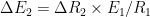
The reader will recognize the green cross as the result of standard extrapolation, which assumes little change in the curve’s slope. But Lord Monckton seems to believe that the feedback theory used in electronic-circuit design requires the abrupt slope change required to obtain the red cross.
We use the circuit below to test that proposition:

Without the feedback path in which the box at the bottom is disposed the circuit would be a linear amplifier, and, since we’re going to assume that R1 through R4 are all 1-kΩ resistors, its gain would be unity. Without the feedback path, that is, the output voltage Vout would equal the input voltage Vin. So Vin corresponds to Lord Monckton’s no-feedback values R, while Vout represents its with-feedback values E.
Note that the feedback path’s input is the entire output Voutvalue. As Lord Monckton put it, that is, “such feedbacks as may subsist . . . at any given moment . . . perforce respond to the entire reference signal then obtaining, and not merely to some arbitrarily-selected fraction thereof.” What we’ll see is that projecting from perturbations instead of entire values nonetheless yields a better estimate.
We could in principle use any nonlinear electronic component for the feedback element, but for the sake of expository convenience we’ll assume that the feedback component we’ve chosen conducts no current when the voltage 


The feedback element’s V–I curve is as follows:

That feedback curve gives the overall circuit the following relationship of input to output:

In a June 22, 2018, video, Lord Monckton contended that a government laboratory’s electronic “test rig” has shown that Lord Monckton’s theory “checks out,” i.e., that the ECS calculation should be based on entire quantities instead of perturbations. Before we use the “single slide” values in this circuit to show that they shouldn’t, we’ll apply a larger no-feedback change to it to show where Lord Monckton gets his extrapolation slope:

As the red dashed line illustrates, his use of entire quantities rather than perturbations means that his extrapolation line passes through the origin. The green dashed line represents using perturbations instead and therefore does not pass through the origin. This fact seems to be Lord Monckton’s basis for contending that climatology assumes the absence of a feedback response the sun’s radiation.
Now we’ll take a close-up view of the smaller, “single slide” change:

We see that the green cross, which represents what Lord Monckton tells us is climatology’s approach, projects the circuit’s output much better than his approach does. This is true even though “such feedbacks as may subsist” in our circuit “at any given moment . . . perforce respond to the entire reference signal then obtaining, and not merely to some arbitrarily-selected fraction thereof.” So nothing about feedback theory requires us to abandon ordinary extrapolation.
This isn’t to say that climatology is right. It’s just that climatology’s error isn’t what Lord Monckton imagines.
Note from Anthony: Personally I believe BOTH arguments to be wrong, for a couple of reasons. But I’ve allowed this post strictly for the purpose of debate.
1. The atmosphere has a chaotic component, with both long and short periods. Linear and nonlinear circuits can’t come close to modeling the atmosphere without having a noise component. It’s just as over-simplistic as the claims by some that we can model any planetary temperature from gravity and atmospheric lapse-rate.
2. Electronic circuits have additional non-linearity built in. For example, operational amplifiers themselves are non-linear internally. They vary their gain with ambient temperature as well as induced temperature from operation. Resistors often have tolerances of 5-10% from their assigned value (in the example above, 1Kohm +/- 10% = 900-1100 ohms) which unless you use special resistors that are high tolerance and temperature stable can’t really represent true linear response in the first place.
3. Seasonal and diurnal variation in Earth’s atmosphere, combined with weather, create a situation where trying to model the Earth’s temperature with an electronic circuit a fools errand. Just look at the variance on Dr. Roy Spencer’s recent graph of the lower troposphere. Looks like a resistor blew out in March and April 2021, doesn’t it?

On a smaller scale, the USA looks even more highly varied in March.

I simply don’t believe ANY simple electronic circuit is capable of accurately modeling atmospheric behavior. Hell, even uber-complex climate models can’t get it right.
I think that Chris Monckton is trying to encapsulate a certain non linearity: Its all very well to do partial differentials but in the grand scheme of things the size of a partial can be affected by the magnitude of the thing of which it is a derivative.
In climate terms, we know that radiated energy is a fourth power of absolute temperature: so the derivative of how much radiative losses vary with temperature changes, varies with temperature!
In similar vein the absorption of energy by greenhouse gasses varies as the log of gas concentration.
You cannot use the partial derivatives obtained at current CO₂ and temperture and extraploate them as constants…
..any more than the gain of a transistor is constant over a wide variation of voltages and currents.
The problem is that climate scientists are not mathematicians, engieers or physicists, They are essentially failures at hard science, looking to make a career out of mediocrity. I mean, really, Michael Mann is actually THICK.
And as for Greta Thunberg…
Mr Smith is right that we do not assume invariance of unit feedback response with temperature. We assume ad interim that it is invariant in the preindustrial era; we then derive the unit feedback response for the industrial era using different data by a distinct method; we find the two unit feedback responses to be a) very small and b) near-identical; and then we assume ad interim that unit feedback response varies considerably with temperature, and find that the latter assumption leads to a material contradiction.
Why so complicated?
https://virakkraft.com/GHE%20feedback.pdf
As I stated upthread, I used your simpler alternative before, at Fig. 12 of https://wattsupwiththat.com/2015/03/12/reflections-on-monckton-et-al-s-transience-fraction/, but some readers found the resultant inversion confusing.
lgl’s circuit inputs to the +ve in terminal rather than the -ve, so it doesn’t invert.
Thanks, and I hope both you and Nick agree using energy is the correct approach because it is meaningless talking about feedback fraction of a temperature and amplifying a temperature. Especially when using 255K as an input when it actually is a result, an output.
Indeed I do, although I have perhaps justifiably been criticized for not emphasizing that enough. I provided deeper and more-mathematical treatment at https://wattsupwiththat.com/2019/07/16/remystifying-feedback/, where I did most of the math in the forcing-to-temperature domain.
Oh – while reading that 5 times looking for an answer, I would appreciate your ‘judgement’ on the following.
Using the numbers from my pdf.
CO2 to 800 ppm -> ‘raw’ energy to the surface is 200+3.7=203.7 which is amplified to 407.4 (400 initially). -> temperature increase at the surface ~1.4 K
My problem is, this is from the ‘live’ system so fast WV feedback is included, and still just 1.4? Where am I derailing?
My apologies; I glanced too quickly at your PDF and saw what I expected: positive feedback. I now see that instead you provided negative feedback only, which limits gain to R_B / (R_A + R_B). Perhaps R_A is voltage-dependent to provide some positive feedback, but that’s just speculation. So my last answer was inapposite, and I’m afraid I can’t answer your last question, because I don’t understand the analogs.
What you call “feedback fraction” isn’t the same quantity Lord Monckton uses that term for. He tends to use it for what the pros I’ve discussed this stuff with call loop gain, which doesn’t mean much in your circuit but would technically be a large negative number.
Your analogs are neither what most folks usually use nor what Lord Monckton (and, for the sake of argument above, I) use. Usually V_in would correspond to forcing, W/m^2, but V_out would global-average surface temperature, i.e., kelvins, and the feedback at your inverting input port would correspond to additional forcing. Your analogs are different, and you seem to be asking me where water vapor is in your circuit. I’m guessing the R_A variation would reflect it somehow, although you use too many acronyms to make out exactly what you’re doing.
Sorry.
I feared that. My setup it too basic for your advanced brain.
It is a positiv feedback loop where the feedback fraction B is determined by R_A/(R_A+R_B) and Gain=1/(1-B) and I’m using energy throughout because that’s how the physics is. The surface warms and radiates energy, not temperature, so no need to convert to temperature and back to energy.
No, the reason why temperature typically gets into the loop is that evaporation responds to temperature, and the resultant water vapor and clouds are what provide the feedback forcing.
Fine, we need temperature to calculate the different energy components, but in a positive feedback loop we want to know how large fraction of the output is fed back to the input, and then we have to look at energy because feedback fraction of temperature is physically meaningless.
I agree with your point about not adding temperatures, and your circuit may be apt, but I can’t see it because I’m still not sure what your analogs are.
For example, I could see it if the signals at your inverting and non-inverting input ports were outgoing and incoming radiation and the output voltage were the surface radiation. That’s not what you’re doing, of course, but exactly what you are doing isn’t clear to me. You write in acronyms that don’t tell me precisely what quantities each of your signals are supposed to represent.
?
200 watts insolation is absorbed by the surface. The surface warms and emits LW. The greenhouse effect (GHE) induces a feedback, represented by RA and RB. (RA and RB is just a voltage divider to set the feedback fraction. You could make that circuit as complex as you like) In this example half of the LW is returned to the surface, resulting in a closed loop gain of 2 and 400 watts LW from the surface. Can’t get more basic imo.
I still don’t understand why Monckton keeps writing things like “the input signal as well as the perturbation is modified by the feedback block”. In a basic positive feedback circuit, which he also keeps referring to, the input does not change. The input is actually the insolation, not emission temperature. The feedback fraction is what changes when CO2 concentration changes.
Thanks for sharing, but, frankly, I’m still having trouble.
The model’s purpose is to study the climate response to a carbon-dioxide-concentration increase, so at least part of the non-inverting input port’s signal needs to be some carbon-dioxide-dependent radiation component. (I can’t say “forcing,” because my understanding is that you want your analogs all to be surface rather than top-of-the-atmosphere quantities.) From your last criticism of Lord Monckton’s exposition, it appears that this isn’t the way you look at it.
If I look upon the non-inverting input port’s signal as, say, net shortwave radiation plus that CO2-related component, then your circuit forces the (water-vapor-effect?) feedback signal at the inverting port to equal that sum. I can’t see how that describes the climate.
As I see it, all you’re doing is amplifying the input signal with a gain of 2. Simple, yes, but I’m not sure it models what we want. So obviously I’m missing something.
Still, there are only so many hours in a day, so I won’t trouble you for a further explanation.
“As I see it, all you’re doing is amplifying the input signal with a gain of 2”
Yes, and that’s all the GHE is doing. If GHE increases then feedback fraction and thereby gain and surface temperature increase.
Mr Born is more familiar with climatology than he is with control theory. If he imagines that temperature feedbacks (the clue is in the name) ought not to be denominated in Watts per square meter per Kelvin of the temperature or warming that triggered them, then he should address his concerns not to me but to IPCC, which will rightly pay him not the slightest attention.
Nick Stokes says –
” Feedback gives a ratio by which changes in the output vary with changes in the input. A necessary consequence is that if there is no change in input, there is no change in output.
But Lord M wants to count in the input the emission temperature, which is, was and always will be. So the output (warming) will depend on that in proportion. But it breaks the rule that unchanging input gives unchanging output. Instead, even if no input changes, emission temperature feedback will provide endless warming. And where does that lead? ”
I think that first statement is technically correct – I have rarely seen Nick get this sort of stuff wrong – but I think he, and many others, including perhaps the author here, are attacking a straw man. That’s not what Lord M is saying. If it looks like he is, it is because he takes as a starting point the assumptions of the modellers, explicit and implicit.
Let me put my understanding as simply as I can –
The water vapour feedback is already there, and operating, in the absence of non-condensing greenhouse gases. The perturbation due to increased CO2 only changes – increases by a small amount – the perturbation that already exists in its absence. Water vapour varies temporally and spatially quite dramatically, whether CO2 is there or not (example, tropical convective cooling cycle). Therefore any calculation of feedback due to a change in CO2 concentration should assume a change to an already existing perturbation, and not a new perturbation. Even more basically, regard temperature change itself as the perturbation, since that is the medium through which CO2 has effect. The input is just one thing – temperature. Not CO2, not WV. Just temperature.
In the real world, that’s self-evident.
Isn’t it?
“Therefore any calculation of feedback due to a change in CO2 concentration should assume a change to an already existing perturbation, and not a new perturbation.”
What is the difference? Every state has a history. The point is that you calculate a gain as the result of a prescribed perturbation to a prescribed state, however it came about.
The input is whatever was initially perturbed.
Mr Stokes knows perfectly well that the input signal as well as the perturbation is modified by the feedback block, and he knows perfectly well that control theory is of universal application to feedback-moderated dynamical systems. Mendacity, therefore, ought to be beneath him.
Mothcatcher is correct at all points. Mr Stokes is – as so often – wrong. And this time I have the impression that he knows he is wrong. The total greenhouse effect of 33 K comprises a) directly-forced warming of about 8 K from natural and 1 K from preindustrial greenhouse gases and b) a total feedback response of about 24 K. Of that 24 K, nearly all is attributable to the 255 K emission temperature, and very little is attributable to the 9 K direct warming from natural and anthropogenic greenhouse gases. But climatology attributes all of the 24 K feedback response to the greenhouse gases, thereby overstating equilibrium warming fourfold, the fraction of warming attributable to feedback tenfold and the unit feedback response 30-fold.
Mothcatcher is (mostly) correct except to assume that I, too, don’t believe that there would be feedback to the sun.
On that point I’ve always agreed with Lord Monckton and disagreed with, e.g., Roy Spencer. However, I think in most cases the disagreement is semantic rather than substantive. Specifically, I’m sure that Dr. Spenser agrees that the phenomenon that Lord Monckton and I call feedback to the sun exists; Dr. Spencer just doesn’t call it feedback. He restricts his use of the term to what I would call a change or disturbance of the feedback.
While I disagree with many aspects of Lord Monckton’s theory, I accept most of it in the head post for the sake of argument. I merely show by that first graph that his theory as summarized in his “end of the global warming scam in a single slide” boils down to bad extrapolation. And I show by the circuit that feedback theory doesn’t justify his bad extrapolation.
As to Mr. Stokes, relevance so infrequently coincides in his comments with intelligibilty that my practice is usually to skip them. I made an exception here because the head post is mine, but he lived down to my expectations.
Mr Born, in order to try to attack our position, takes out of context a slide from a 3-year-old presentation. At least he has now conceded explicitly that the emission temperature derived from the surely observable fact that the Sun is shining will itself engender a feedback response. Since the emission temperature is 30 times larger than the direct warming by natural and anthropogenic greenhouse gases, most of the feedback response currently allocated to greenhouse gases is actually attributable to the Sun. Therefore, final or equilibrium warming by greenhouse gases will be smaller than climatology currently admits, because climatology adds the emission-temperature feedback response to, and miscounts it as though it were part of, the feedback response to direct warming by noncondensing greenhosue gases.
Nothing in that description requires any assumption that the unit feedback response will be invariant with temperature. We begin by assuming ad interim that in the preindustrial era it is, and then we use an entirely distinct and well-established method, the energy-balance method, on entirely distinct data for an entirely distinct period, the industrial era, to derive a midrange estimate of the industrial-era unit feedback response. The two unit feedback responses are very small, and very close to one another, and they suggest that, if anything, unit feedback response is actually getting smaller with temperature – which is precisely what official climatology assumes. This comparison of the two unit responses suggests that there may not after all be much variance of unit feedback response with temperature.
Then we assume, again ad interim, that the unit feedback responses to emission temperature and to direct greenhouse-gas warming are different. It is then a simple calculation – which no one in official climatology seems to have bothered to attempt before – to show that to justify a midrange ECS of 3 degrees the unit feedback response to greenhouse gases would have to be 50 times the unit feedback response to emission temperature. There is no plausible physical reason for so large and rapid a growth in unit feedback response in what is a near-perfectly thermostatic system.
But we don’t stop there. We then actually calculate the apportionment between the feedback responses to emission temperature and to the preindustrial noncondensing greenhouse gases, using various assumptions of the rate of variance in unit feedback response with temperature.
Very nearly all of this research has not been published, for the good and sufficient reason that it has been under peer review at a leading journal for six months. If there were anything as obviously wrong with it as Mr Born would like us to imagine, the paper would have been thrown straight out at the beginning.
Mr Born has, therefore, attempted – not for the first time – not only mendaciously to mischaracterize our research, misleading Anthony Watts into thinking us half-witted, but also to attempt to review a very considerable body of research that he has not even seen. Anyone genuinely interested in the objective scientific truth would not misbehave as grossly or as dishonestly as that.
Now Lord Monckton objects that I’ve taken his slide above “out of context.” Well, let’s consider the context.
In 2018 WUWT ran a Lord Monckton post about his theory. It contained a long objection-and-response-style description, at the end of which he summed it up with that slide, presenting it thus: “Here’s the end of the global warming scam in a single slide. The tumult and the shouting dies: The captains and the kings depart … Lo, all their pomp of yesterday Is one with Nineveh and Tyre.”
That slide encapsulated two videos and six previous WUWT posts on his theory, in the first of which he had described the theory as the product of research that had been going on for eighteen months.
That’s the context. The slide wasn’t some throwaway. It was his triumphant summary of all that had gone before. It was “the end of the global warming scam in a single slide.”
Except that it was wrong.
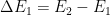
That slide showed how he said Hendrik Bode and control-systems theory dictated that ECS (“ΔE_2”) be calculated from pre-industrial and current temperature values E_1 and E_2, the values R_1 and R_2 that those temperatures would have taken without feedback, and the temperature change ΔR_2 that doubling CO2 concentration would cause without feedback.
As any high-school analytic-geometry student would be able to verify, the two black dots and the red cross on the first plot above represent that slide’s quantities graphically, the vertical distance ΔE_2 between the red cross and the lower black dot being the ECS value Lord Monckton said the “Bode equation” required. The student could also see that the method thereby illustrated boils down to bad extrapolation.
And what Lord Monckton called climatology’s “startling error of physics” is represented by the green cross. That “startling error” is what high-school kids all over the world would recognize instead as proper linear extrapolation.
Now that the plot above lays out for all to see that Lord Monckton is the one who made the startling error, he dismisses what he then called “the end of the global warming scam in a single slide” as being three years old.
Why does its age matter? What happened in the past three years to change things?
Did they repeal what Lord Monckton calls the “Bode equation”? If he no longer stands by his “end of the global warming scam in a single slide,” when did he discover his mistake? At what point did he tell his gushing fanboys they’d been misled?
Lord Monckton should have admitted his error a long time ago. It’s not as though no one had pointed it out. Many had, including me at, for instance, https://wattsupwiththat.com/2019/06/03/reporting-the-fraudulent-practices-behind-global-warming-science/#comment-2715071.
Lord Monckton’s past behavior has shown him to be a dishonest interlocutor, so I won’t take the time to correct the rest of his comment. But the fact that he could make so fundamental and clear an error in high-school math but persist in refusing to admit it after it’s repeatedly been pointed out to him tells you all about him you need to know.
Mr Born is, as usual, incorrect and his tone is malicious. His post here was a response to a posting by me a few days back. However, he could not fault that posting, so he decided to try to fault a slide from a three-year-old posting instead.
He has known, ever since I pointed out the large error in his earlier whigmaleerie posting, that we are right about the fact that the Sun is shining and that, therefore, it generates a substantial feedback response, which accordingly diminishes the greenhouse-gas feedback response.
He had not realized that his extrapolation voodoo implies a unit feedback response to greenhouse-gas warming that exceeds the unit feedback response to emission temperature by two orders of magnitude.
Even though he knew from my posting of a few days back that we derive the unit feedback response in two distinct ways and find that it varies very little, he was so childishly desperate to find fault where none existed that he ignored that context deliberately and with the characteristic mendacity of the Born Liar.
Still, his nasty style has shown many here that he is acting in the worst of bad faith, and shows no interest in the objective truth.
Note how Lord Monckton has ducked my questions about what had changed to make his slide from three years ago inapplicable. It’s obvious why he won’t admit the error in that slide I pointed out above. Contrary to what he claims, I have no trouble similarly finding fault with his most-recent post (https://wattsupwiththat.com/2021/05/09/why-models-cant-predict-temperature-a-history-of-failure/), because that post’s fourth, “feedback loop” diagram makes the exact same error I pointed out above: basing extrapolation on average rather than local slope.
If you go to that diagram’s lower left, you’ll see that it presents (255+8+24)/(255+8) as the “corrected” extrapolation slope. But that value is the average slope, whereas standard extrapolation would use local slope. As my last two plots above demonstrate, the local slope, whose use Lord Monckton denounces as a “startling error of physics,” does a much better job. In contending otherwise, Lord Monckton has for over three years been making an obvious error in high-school math.
Again, there’s no point in attempting a reasoned discussion with him, so I’ll probably ignore any further falsehoods he perpetrates in this thread. But here’s a tip: assume as a default position that he doesn’t know what he’s talking about. I became acquainted with control-systems theory when he was still a schoolboy, and I can assure you that he has been misrepresenting it for years now.
If those suspiciously unnamed controls-system theorists whose authority he invokes believe anything like what he says they do, they’re third-raters at best. Why doesn’t he let them and their credentials come out from behind the curtain? I’d be happy to take them on.
Mr Born is incapable of understanding the characteristics of a system overwhelmingly dominated by a large input signal and the feedback response thereto. Nor does he grasp his central error, which is to ignore the fact that in such a system the ratios of unit feedback responses provide useful constraints on system variance.
He treats the climate as an abstraction. We do not.
Worse, he continues to attempt to comment on research he has not seen – research that has been with a journal for peer review for six months. If there had been so obvious and so glaring an error in our research as that which he longs for, the paper would have been thrown back, but it has not been.
He has based his posting not on my own recent posting but on a three-year-old slide that indicates ECS is of order 1 K. Our continuing research confirms that result – and the near-invariance of unit feedback response with temperature – by several independent methods, most of which we have not published because they are under peer review.
The old radio operators would tune their transmitters for maximum smoke. 😉
“I simply don’t believe ANY simple electronic circuit is capable of accurately modeling atmospheric behavior.”
I think I understand the attempt as a metaphor, and I’ve seen better engineers than I make the analogy work in whatever it is that we call real life. But mixing digital electronic logic with logical reasoning is full of pitfalls. I think the author uses electronic/physics calculations to prove that his own circuit doesn’t look like Monckton’s description, without realizing that Monckton is stating that the metaphor is false. Electronic models of feeback aren’t applicable to climate modeling. The author proves what I understand to be Monckton’s point.
More at my own level of understanding is that positive feedback causes a system to cycle or amplify signal out of control, and negative feedback can be used to control output. Neither can be described precisely without an exact and thorough understanding of most of the overall system. Metaphors drawn outside of the system from inside the well understood system are most likely to fail because the systems are different. Climate seems to me a poorly understood, quite complex, and complicated system, that exhibits behaviors that are also poorly understood. I can’t get to understanding climate from electronic circuitry metaphors. I also can’t get an understanding of the climate system based on positive feedback from out-of-context calculations of esoteric properties of a trace element.
I can understand that a model test rig might be another software driven computer model, and not a bench device.
But I am just an retired obsolete specialist engineer, a specialist technision of retired equipment, an aspirational curmudgeon, a carbon demonology apostate, and a climate change infidel, what do I know?
“without realizing that Monckton is stating that the metaphor is false. Electronic models of feedback aren’t applicable to climate modeling.”
So who claims the metaphor is true? It seems to be the ultimate straw man. It doesn’t come from climate scientists; it has nothing to do with the way GCMs work.
It was Lord M who actually built a circuit, claiming that it disproved something or other.
I really thought that the test rig in Monckton’s description was shorthand for a simulated software climate model, and not circuitry. I stipulate that my impression is incorrect.
On the other hand, neither test rig circuit causes an output that reproduces the actual measured temperature data curve, so I still believe that Born proves Monckton’s point. The feedback formulation in climate modeling is based on a misapplication of principles that describe real electronic feedback, and have nothing to do with the climate.
Curmudgeonly yours,
dk_
“The feedback formulation in climate modeling…”
Climate models do not use any feedback formulation.
Dk_ is right and Mr Stokes – as so often – wrong. Our simple feedback-amplifier circuit was built to confirm that in the presence of non-negative feedback the feedback block will modify not only perturbations of the input signal but also the input signal itself. The emission temperature driven by the Sun is the input signal, and, yes, it drives a far larger feedback response than the direct greenhouse gas warming does, for emission temperature is 30 times larger than the direct warming by greenhouse gases. But climatology adds the large emission-temperature feedback response to, and miscounts it as part of, the actually minuscule feedback response to direct greenhouse-gas warming. An electronic circuit is more than capable of confirming that simple but important point.
Dk_ is not quite right. Control theory is of universal application to feedback-moderated dynamical systems. Therefore, certain aspects of all such systems may be demonstrated by one such system that is controllable and readily mensurable – an electronic circuit. Our electronic circuit was built to confirm what actually needed no confirmation: namely, that any feedback processes that subsist in a dynamical system will perforce act upon, and modify, not only a perturbation of the input signal but also the input signal itself. I am frankly baffled that Mr Watts would imagine for a single instant that the distinguished team of eminent researchers that I have had the honor to gather about me would be naive enough to think that a simple linear feedback amplifier would be capable of demonstrating all the nuances and irregularities of the chaotic object that is the climate. But it is capable of demonstrating the surely simple and surely undeniable point that there is a large feedback response to the fact that the Sun is shining; that that feedback response would be present even in the absence of any perturbations of the direct warming by the Sun; and that, therefore, it is a grave error to add the feedback response to the Sun’s heat to, and to miscount it as part of, the actually minuscule feedback response to the direct warming from the Sun.
And one more point in response to Dk_. He says he thinks positive feedback always leads to oscillation. No: it does so only where the feedback fraction – i.e., the fraction of the output signal that is represented by feedback – is close enough to unity. Since we find the feedback fraction to be more like 0.1 than 1, there is no expectation that feedback-induced oscillation will arise. There is no danger of the “tipping points” imagined by climate fanatics.
Accepted. I based my idea on admitted shaky and long-stored knowledge and probably an oversimplification of audio amplification. Attempting to reasoning “out loud” gets one noticed, is often embarrassing, but sometimes leads to learning, even occasionally in an aspiring curmudgeon. I will try to produce more. Thanks.
Ha ha ha. This thread is a train wreck of bullsh*t. What matters in the end is the statement at the end of the article….
”I simply don’t believe ANY simple electronic circuit is capable of accurately modeling atmospheric behavior. Hell, even uber-complex climate models can’t get it right”
To which I would add, no-one has the slightest clue what’s happening, but lots of people don’t have the slightest clue in a much more complicated way.
10/10 for trying though!
Mike appears to be laboring under the same delusion as our kind host, who – bafflingly – imagines that the distinguished team of climate researchers that I have the honor to convene would for a single instant think that a simple electronic circuit is capable of representing all the ins and outs and ups and downs of the complex, nonlinear, chaotic object that is the climate. A simple circuit is, however, capable of demonstrating the simple point we make – namely, that even in the absence of a perturbation in the shape of direct warming by greenhouse gases the emission temperature itself will drive a large feedback response that is currently and erroneously added to, and miscounted as though it were part of, the actually minuscule feedback response to direct warming by greenhouse gases. In consequence of climatology’s error, the system-gain factor and consequently equilibrium sensitivity is exaggerated approximately fourfold, the feedback fraction (the fraction of equilibrium temperature or sensitivity represented by feedback) is exaggerated tenfold, and the unit feedback response is exaggerated 30-fold.
So no arguments as to the validity of this or any other circuit model then? Wonderful!
It is not entirely clear that Mike is being serious, but I shall reply on the assumption that he is. We built our own circuit, and ran it, and it confirmed the long-established, definitively-proven theory relating to simple feedback amplifiers. In particular, it confirmed that there is a feedback response not only to any perturbation of the input signal but also to the input signal itself. Then we called in a government laboratory to design and build its own circuit and, after months of toing and froing so as to overcome the difficulties caused by the fact that the perturbation in such a circuit representing the climate is so very small in relation to the input signal (the operator’s presence in the room altered the way the circuit behaved), we were eventually able to obtain the required confirmation.
None of this was in any way necessary, because the relevant elementary linear algebra is straightforward. But we did it anyway, because every climatologist with whom we have discussed this has been astonished at the notion that nearly all of the feedback response in the climate system comes from the Sun and not from the noncondensing greenhouse gases.
The circuits were, therefore, validated by the government laboratory, which consented in writing to the conclusions we have drawn from the operation of its circuit.
For my money thr circuit shown in this article is more complex than it need be, which raises suspicions.
The circuit has two op amps with feedback on the inverting inputs. WHY???
All that is required is a single op amp with feedback on the non inverting input.
In point of fact, this circuit could be modelled with a single transister (or op amp), 1 fixed resistors, to simulate the earth and 2 variable resistorx to simulate the sun and CO2.
Add in a battery as a power supply and put an ammeter in series with the earth resister to measure temp, or place a voltmeter in parallel with the earth resister to measure temp.
Now vary the values of your two variable resisters. Record their values with an ohm meter and the resulting “temperature” of earth.
Plot values of sun, co2, and earth. This will tell you who has it right.
Or if you know excel, simply construct the whole thing on a spreadsheet., which alows you to completely remove any non linear response. Graph the result and you have solved the mystery.
Note: the second variable resistor represents ghg, not just co2, so it also includes h20.
I think it is because the feedback network is a current source, which can’t be jammed into the positive input of a non-inverting op amp.
But it can be jammed into the base of a transistor, because you can select PNP or NPN depending on the circuit.
Also it has been mant years, but i dont recall a problem using op amps one way or rhe other, depending on whether you are pulling the load high or low.
For planet earth resistor, ground would likely be space and you would try and pull this high to repeesent the sun and feedback, but really is just convention.
Electrons flow from ground to the positive supply, due to and error long ago that has never been changed. At one piint it was assumed electricity flowed from positive to negative, before the electron was discovered.
The input impedance of an op amp is extremely high because they are typically connected to the gate of a MOSFET. His circuit diagram shows the feedback current I_f=KVaf. If he had used the non-inverting topology, I_f would have been exactly zero. As drawn, the feedback current splits between R1 and R2.
The circuit is more complex than it need be which raises suspicions.
A positive feedback resistor 1/10 the value of the input resistor on the non inverting input wilk give you a pretty good model of the earth.
The input resistor being the sun, the feedback resistor ghg and the load resistor being the earth.
The biggest problem is the high gain on the op amp. You need to select something like a 100k resistor for the sum, a 1000k resistor for ghg. The earth resistor is less critixal, maybe 10k.
Another approach would be a single transistor with positive feedback. In this case you probably cant use DC because of the 0.6V diode drop across the junction.
Rather you probably need an AC signal and capacitors to remove the DC component.
Note2: since you are modelling temperature and radiation you probably need to take the 4th root of the current thru or voltage across the earth fixed resistor. But this wont change the results.
We should not lose sight of the real problem and the reality of its conditions. The argument that water vapour causes a positive feedback is a reasonable one. The logic that CO2 causes some warming and a warmer atmosphere holds more water vapour is not in doubt.
The argument that positive feedback is unlikely also has some merit. Over millions of years the atmosphere has had several thousand ppm of CO2. There is no evidence that the instability of positive feedbacks caused frequent frying of evolving life forms.
So what is going on? I keep pointing out that this is a spectroscopy matter and spectroscopy offers the answer. The absorption bands that matter are dominated by water vapour and to a lesser extent by CO2. The bands are effectively saturated. This means that most of the IR at these wavelengths has already been absorbed by these gases. Adding more of these gases is not going to make a huge difference. We are in the region of diminishing returns and that applies to water vapour as well as carbon dioxide. So, yes, there is some positive feedback but the impact (heating effect) is very small.
This is the reality of the situation and it is verifiable experimentally using IR spectroscopy. All the work has been done and the data is in the HITRAN database.
The wider implications are enormous. No matter how much of the common greenhouse gases enter the atmosphere, we will not get serious warming ( They share the bands with water vapour which dominates the absorption and almost no more IR absorption is available.)
This explains a great deal about the stability of our climate and the “goldilocks” suitability for life to thrive, especially when high levels of CO2 encourage plant growth. It also explains why climate models cannot deal with this matter. Their creators are incapable of contemplating that the all powerful greenhouse effect might actually be self limiting and that we have already reached that limit. Mother Nature runs rings around these people.
Yes, one can show by spectroscopy that ECS will be small: Will Happer has done so. However, one can also show why it is that the modelers thought it would be large. They forgot the Sun was shining and did not realize that the emission temperature of 255 K would drive a large feedback response. It is a great deal easier to prove climatology’s error in adding that large emission-temperature feedback response to, and miscounting it as part of, the actually minuscule feedback response to direct greenhouse-gas warming than it is to prove by spectroscopy that climatology has exaggerated ECS.
Sorry if it has already been pointed out, but Joe’s circuit if built would blow up. A small matter of positive feedback. Getting rid of the second amplifier, or adding a third, would solve the problem.
Such a howler does cast doubt on the argument that Joe is attempting to adduce.
Here is what I get from his diagram, hopefully the signs are correct:
R1=R2=R3=R4=R
V1 = output of op amp 1
V2 = output of OA2 = -V1 = Vout
current through R1: I1 = Vin/R
current through R2: I2 = V1/R
feedback current: If = KaVout
summing currents at the inverting input of OA1:
I1 + If = I2
Vin/R + KaVout = -Vout/R
Vout/R + KaVout = -Vin/R
Vout(R+Ka) = -Vin/R
Vout = -Vin R/(R+Ka) = Vin (-1(1 + Ka/R))
A very strange circuit.
Monte,
I see you were brought up in the transistor era. Op Amp computing technology was born in the valve era, using voltage as the basis for programming as opposed to current for transistor circuits. .
The point of an Op Amp is that the input represents a virtual earth, at the point of connection between an input resistor and a feedback resistor connected to the input of a very high gain linear amplifier. The ratio of the resistors sets up the gain of the circuit.
Taking an input of say +10 volts, and an input resistor of say 10k ohms, a gain of two requires the feedback resistor to be 20k ohms. The amplifier will then need to output -20 volts so that, the -ve input of the amplifier will then be at zero volts, or in other words a ‘virtual’ earth.
Note that the output polarity will be inverted.. a so-called ‘negative feedback’
If you look at Joe’s circuit, the whole thing will likely burn out straightaway, because a double inversion through the two amplifies will result in overall positive feedbaclk and a runaway condition.
All very straigntforward really, and it was a delight to work on the design and commissioning of analogue computers. including massively complex full mission flight simulators, because it was all understandable and obvious what was going on.
Not really—the high input impedances of the plus and minus inputs mean that the current into them is essentially zero, and when operating linearly, the voltage across the plus and minus inputs is essentially zero as well.
It is a “virtual earth” only if one of the inputs is connected to a zero voltage reference, but there is no requirement that this be so.
“If = KaVout”
No, KVout^a.
And it had to be a little “strange” to match the numbers in Lord Monckton’s slide.
Your writeup made this clear as mud.
What is the magnitude of a?
a = 2.626611
K = 1.140583e-08
I’m curious. Just what was it that you didn’t understand about the paragraph immediately that preceded the diode-resistor ladder and the V-I curve that followed it?
How do you calculate these values to seven significant digits?
Vout + RK(Vout)^a = -Vin
You can’t solve for Vout without doing something like a Taylor Series expansion.
This circuit doesn’t do what you think.
You forgot the negative sign on Vout.
And you don’t need to solve for Vout. Just assume Vout and solve for Vin. The only problem is that you could come up with some unstable-state solutions.
If you insist on going the other way, I suggest successive approximation. It has the advantage of detecting instability.
I remain of the opinion that the circuit does what I said.
You call this a non-linear feedback. Yet once the forward bias point of the diode is reached the current through the diode is essentially linear. For a silicon diode there is a small interval, typically between 0.6v and 0.7v where there is actually a curve associated with the forward current. After about .75v the current curve becomes linear.
Your graph shows the forward current to be a curve all the way from the forward bias point to the extreme of the graph. This just isn’t so in the real world.
The point of the post wasn’t electronics; it was that for extrapolation of a nonlinear function the local-slope use Lord Monckton criticizes works better than average-slope use he advocates and that nothing about feedback changes this high-school-math fact.
As I said in the head post, the particular nonlinearity chosen to demonstrate this fact doesn’t much matter, and a diode-resistor ladder would only approximate the particular V-I function I assumed for expositional convenience. I never contended that such a circuit would be very practical, at least without some voltage scaling. Moreover, since I haven’t so much as picked up a soldering iron since the Vietnam War, I didn’t intend to provide a tutorial on basic electronics.
That said, if someone (inexplicably) wanted to build such a ladder circuit, the approximation could be pretty good, although without scaling it would take over eight hundred silicon diodes and resistors.
I’m guessing that doing the Shockley-equation calculation for such a circuit could be tricky, but you could get a rough approximation by modeling the diodes as conducting negligible current below the diode drop and offering negligible small-signal resistance above it. What I think you’d find is that without scaling the resistances would decrease from about 28 megohms on the right to about 0.5 megohm on the left.
In operation, the current would largely flow only through the high-value resistors on the right when the voltage is low, because the lower-valued resistors on the left are connected in series with a large number of diodes and thus more diode drops. As the voltage increases it exceeds more diode drops and thereby causes significant flow through more lower-value resistors.
But there’s no need for readers who aren’t familiar with circuit analysis to worry about the electronics. Just concentrate on Lord Monckton’s “end of the global-warming scam in a single slide” and the plot I used about to illustrate it.
Don’t forget to mention how you used the graph way outside of its context.
You didn’t address my main point. What you have described is basically a step function, not a non-linear function. The function is essentially zero below the diode cutoff and linear above the diode cutoff.
You only get a difference in your graph because you assumed an exponential curve instead of a linear curve past the 0.6v breakover point.
It’s difficult to get a non-linear feedback loop with only passive devices. In fact, I’m not sure exactly how you would do it with only passive devices. You really need an active element whose transfer function is either exponential or is of a higher order than 1 (i.e. linear).
I’m not sure where in the Earth’s thermodynamic system you would find a non-linear feedback. The sum of linear components is still linear, just with a different slope. Different slopes on linear processes do not sum to non-linear results.
Look, I’ll try this once more, but that’s all, because it doesn’t appear that you’re going to get it.
Contrary to your assertion, I actually am approximating each diode by a “step function” as you call it: I assume that each diode’s dV/dI is infinite below one diode drop (I used 0.7, you used 0.6, but it doesn’t matter for present purposes) and zero above one diode drop.
With this idealized step-function component, consider a ladder consisting of three diodes in series shunted by respective 1k resistors. Now let’s apply an input voltage. Below 0.6 volt the total shunt current is zero because we assumed that dV/dI is infinite in that regime. But at 1.2 volts the total shunt current is 0.6 mA because the first diode is conducting. At 1.8 volts it’s 1.8 mA. At 2.4 volts it’s 3.6 mA.
So you see that the composite feedback component’s V-I characteristic is nonlinear.
As to other nonlinear passive devices, please look up tunnel diodes.
I’m sorry, but it doesn’t appear that further attempts on my part will be fruitful. We’ll just have to agree to disagree.
Sorry I failed to notice some of the electronics questions. Just in case anyone’s still paying attention, I’ll belatedly respond.
Actually, nothing much depends on the electronics, but, since Lord Monckton went on so much about his “test rig,” I provided one. All you really need to know to follow the argument is that the circuit’s output as a function of its input is as plotted above. Since some folks have put some electronics misinformation in this thread, though, a little explanation:
First off, I’m not sure I understand the complaints about complexity; the circuit is simply a single unity-gain amplifier and a nonlinear feedback element. By depicting the circuit at the op-amp level I made the analysis simpler than it would have been at the constituent-transistor level.
The only (mildly) tricky part was so picking a feedback-element characteristic as to match the numbers in Lord Monckton’s slide. The exponent a I used for that purpose was 2.626611, and the coefficient K was 1.140583e-08 .
Yes, I could have implemented the amplifier in a single op amp instead of two, but I know from experience that some readers would have objected to the resultant inversion.
And, no, unless the input voltage gets too high, the positive feedback won’t make the circuit “blow up.” Here’s the circuit analysis:
Let’s call the nonlinear element’s voltage-to-current ratio Rf (a variable quantity that depends on Vout). As was stated above, all the other resistances are equal to one another, making the two-op-amp combination a unity-gain amplifier. Therefore the first op amp’s output is the negative of the second’s, i.e., of Vout’s.
Also, the first op amp’s inverting input port is a virtual ground, so we can sum the currents flowing into that node as follows: Vin / R1 – Vout / R2 + Vout / Rf = 0.
Solving for Vout gives us Vout=Vin Rf R2 / (Rf – R2) / R1.
Consequently, Vout remains finite so long as Rf exceeds R2, as it will throughout the operating range of interest. Specifically, the loop gain won’t reach unity unless the input voltage reaches the value indicated by the output-vs.-input diagram’s vertical dotted line.
Again, my apologies for the slow response.
Mr Born’s circuit is entirely irrelevant, for it reveals absolutely nothing that in any way bears upon, let alone demonstrates any error in, our research.
He has long known that we relied upon the circuit built by a government laboratory to establish a few simple fact – facts that even he cannot deny. Chief among these is the fact, which the head posting somehow fails explicitly to state, that in any feedback-moderated dynamical system there will be a feedback response not only to any perturbation of the input signal but also to the input signal itself.
In the climate, the input signal is the emission temperature that would be present near the surface because the Sun is shining, even if, at the outset, there were no greenhouse gases in the air at all. Since that input signal is about 30 times larger than the perturbation by greenhouse gases, a substantial fraction of the total feedback response that climatology accords exclusively to the perturbation is in fact attributable to the Sun.
Mr Born has also long known that in the real climate – an essentially thermostatic system – there are very powerful constraints on the rate of variance of unit feedback response to the reference signal (direct temperature or warming) with temperature. Not the least of these constraints is the fact that emission temperature is at least 255 K and the perturbation by greenhouse gases is only 8 K.
If, for instance, there was no variance in unit feedback response, then the system-gain factor – the ratio of direct warming before feedback to eventual or equilibrium warming after it – would be about 1.1 after correction of climatology’s error in neglecting the large feedback response to emission temperature – the temperature that dominates the system. Then, since the direct warming by doubled CO2 is little more than 1 K, the final or equilibrium warming in response to doubled CO2 – ECS – would be about 1.1.
But let us suppose that the feedback response to direct greenhouse-gas warming is not just a little greater than the feedback response attributable to the observable but neglected fact that the Sun is shining but up to five times that emission-temperature feedback response.
In that event, ECS would not be more than 1.5 K, and only then on the assumption that emission temperature is as low as 255 K. But it can’t be as low as that, because, as Professor Lindzen pointed out a quarter of a century ago, climatology has forgotten there are clouds in the sky, which would not be there at emission temperature because, at the outset, there would be no greenhouse gases (and specifically no water vapor) in the air. Correct for that error and emission temperature becomes 271 K. Then, even if the unit feedback response to greenhouse-gas warming were five times the unit feedback response to emission temperature, ECS would be only 1.2 K.
Even if per impossibile the unit feedback response to direct greenhouse-gas warming were ten times the feedback response to emission temperature, and even if per impossibile emission temperature were as low as 255 K, ECS would be just 1.8 K, less than half the 3.7-3.9 K midrange estimate that current models imagine.
Mr Born knows all this because, in my response to his earlier article showing his favored curve of the evolution of variance in unit feedback response with temperature, I drew his attention to the fact that his curve implied, altogether impossibly, that unit feedback response to direct greenhouse-gas warming must be as great as 90 times the unit feedback response to emission temperature.
And what if we derive the system-gain factor and consequently ECS from the latest industrial-era data by the well-established energy-balance method? Note that both the data and the method are entirely distinct from the preindustrial data and method. Sure enough, the midrange ECS comes out at 1.1 K, exactly as it does using the preindustrial method corrected for climatology’s error.
That would suggest – to anyone other than Mr Born – that there is very little variance with temperature in the unit feedback response.
But we went further. We found that the original rate of medium-term anthropogenic warming predicted by IPCC in 1990 on the basis of climatology’s error was about 2.4 times the actual anthropogenic warming. Then we converted the predicted medium-term warming to degrees per century equivalent, so that we could compare it with climatology’s current predictions of ECS (which are broadly equivalent to a century of anthropogenic warming from all causes).
IPCC, instead of reducing its predicted midrange ECS by at least half, as it has done with its medium-term warming prediction, has actually increased it, so that it is now three or four times the 1.1 K warming that is our current best estimate (compared with our 1.2 K estimate of three years ago).
The horrifying truth is that Mr Born, who is not any sort of control theorist, has arrogantly assumed that he knows better than the team of control theorists, including a tenured professor in the subject, who are among my co-authors, and who keep us straight on the ins and outs of feedback formulism.
Worse, Mr Born has repeatedly sought to pass judgment on research that he has not even read. That, on its own, should alert the discerning reader to the regrettably malevolent but entirely valueless approach he has adopted.
If we had really perpetrated the crass error of which Mr Born continues – with increasing desperation and futility – to accuse us, one wonders why it is that the previous two journals to which we submitted our paper were not able to find any significant or uncorrectable fault with it; why it is that the editor of the latter journal wrote to us to say that we had answered all the reviewers’ comments to his satisfaction and thought that our paper merited publication but that his fellow editors would not allow this or any such paper to be printed; and why it is that the editor of the current journal to which we have submitted our paper, who has had it for six months and had previously publicly declared that skeptics have no credible arguments against the official catastrophist narrative, has not thrown the paper back at us.
Mr Born ought to have had enough common sense to realize that, even if it amuses him to imagine that I am as stupid as he suggests, my distinguished co-authors are not; the reviewers of our paper are not; the editor who accepted that our paper is sound is not; and the current editor, who has not rejected out paper, is not.
Little though the true-believing Mr Born may like it, in reality climatology has made a very large error indeed, and a strikingly elementary one. The fact that Mr Born, despite the evidence, cannot bring himself to admit this is regrettable.
What is more, climatology has perpetrated the very error of which Mr Born accuses us, and the fact that Mr Born, instead of directing his spite and ire at climatology, directs it at us instead does not speak well of his independence of mind, still less of his motives.
To take one example, of which we can prove Mr Born is aware, Lacis et al. (2010, 2013) state that three-quarters of the entire greenhouse effect is feedback response to the other quarter, which is direct warming, so that the system-gain factor is 4.
And climatology, for this very reason, imagines that today’s system-gain factor is about 4. Not much variance with temperature, then, is there? Mr Born has wasted his time and his hatred to no purpose. But we must love him dearly all the same, for he has provided harmless, if wrong-headed and ill-motivated, entertainment. And, in the economy of salvation, even evil has its place.
Even if you are right I don’t see why it would “end the climate emergency”. For that to happen you would have to show that this “grave error” is built into the models. I’m quite sure a simple feedback loop is not the fundamental building block of GCMs. The models estimate that feedback1 will add x, feedback2 will add y and so on to the temperature. Then we can take that output and calculate the implied feedback and gain, after simplifying the whole system down to a amplifying feedback loop. Using the mainstream definition of gain we will get one value. Using your definition we will get another value. So what? In Hansen et al 1984 they even managed to mix up feedback with gain, defining feedback as f=1(1-g), getting what they called feedback factors of 1.x and gains of 0.y.
Igl is not quite right. The feedback error is not “built into the models”, for they do not use feedback formulism at all: instead, as the head posting explains, they try – and fail – to solve the Navier-Stokes equations in computational fluid dynamics for half a million atmospheric cells in a succession of time-steps. And they fail to allow for propagation of error from each time-step to the next. Therefore, their predictions are mere guesswork.
Our method requires no knowledge of the internals of the models, which we treat as a black box. We know the key inputs to the models, and we know their key outputs. And those outputs are consistent with climatology’s error in ignoring the large feedback response to emission temperature, and inconsistent with the correct approach, which is to deduct the emission-temperature feedback response from total feedback response to yield the very much smaller feedback response to direct warming by greenhouse gases.
The corrected result thus serves as a yardstick or benchmark against which to measure the absurd exaggerations in the models. And that is why, when the Vice-Chancellor of the University of East Anglia saw an earlier version of our paper, he called a meeting of the entire environmental-sciences faculty and yelled at them that they had better refute it or the fat government grants for research into climate change would dry up. They couldn’t refute it, of course.
The reason why it matters that ECS is only 1 K and not 4 K is that the corrected value on any view harmless and net-beneficial, while the erroneous currently-imagined value might or might not be harmful.
Another value of correcting this particular error by climatology is that it is a very large and very simple error. Naturally, the army of true-believers, such as poor Mr Born et hoc genus omne, are doing their best to make it look very complicated. But it isn’t. The Sun is shining. The emission temperature is so large that even if its unit feedback response were less than the unit feedback response to the 8 K direct greenhouse-gas warming by a factor of ten ECS would only by 1.8 K, half the currently-imagined 3.9 K.
In fact, however, the system is thermostatic and, precisely because the feedback response to emission temperature is so large compared to the entire warming effect of greenhouse gases, ECS cannot be anything like as large as climatology imagines.
Monckton: +1 K IPCC: +3 K G=1/(1-B) B=-1/G+1
T0=255 T1=288 T2=289 or 291 T1: today T2: after 2xCO2
Today: G=288^4/255^4= 1.63 B=0.387
Monckton: G=289^4/255^4 =1.65 B=0.394
IPCC: G=291^4/255^4 =1.70 B=0.410
How can you use an electronic amplifier to prove B will increase from 0.387 to 0.394 and not to 0.410 ?
(I’m still using energy because to me it’s silly to amplify temperatures, and I still mean 255K is wrong but enough on that)
In response to Igl, we do not use an electronic feedback amplifier to prove what Igl says. We use it solely to demonstrate that even in the absence of a perturbation of the 255-271 K input signal, such as the 8 K direct warming by (or reference sensitivity to) preindustrial noncondensing greenhouse gases, the input signal itself will provoke a feedback response – and a substantial one.
Of course, there is no need for any such demonstration, for the elementary equations describing the feedback amplifier are sufficient in themselves. We got the national lab to build the test apparatus to demonstrate to climatologists, who were surprised by the notion of a feedback response to anything other than the perturbation, that there is such a response.
For R the 255 or 271 K reference signal, delta-R the 8 K direct warming by preindustrial noncondensing greenhouse gases, E the 287 K output signal, f = 1 – (R + delta-R) / E the feedback fraction (i.e., the fraction of E attributable to feedback response), A = E / (R + delta-R) the system-gain factor and B = E – (R + delta-R) = Ef the feedback response, the equations are as follows:
E = (R + delta-R) + B = (R + delta-R) + Ef
(R + delta-R) = E – Ef = E(1 – f)
A := E/ (R + delta-R) = 1 / (1 – f)
I have emboldened the input signal R, the emission temperature, throughout so that Igl can see exactly why it is that the feedback response B is a response not merely to delta-R but also to R itself.
Temperature feedbacks are denominated in Watts per square meter of the temperature or warming that triggered them, so that the feedback loop calculations are necessarily done in Kelvin, but if Igl would prefer other units his quarrel is not with me but with official climatology, all of which we have adopted ad argumentum except what we can prove to be in error.
Thanks. That bit is fine, but I still think you have to show the amplification of the 8K only to the full 33K GHE is built into the models.
IgL asks that I should show that the direct warming of 8 K by greenhouse gases becomes the 33 K entire greenhouse effect in the models.
Simple:
The doubled-CO2 forcing in the models is 3.52 W/m^2 (Zelinka et al. 2020, mean of the CMIP6 models)
The Planck sensitivity parameter is 288.5 K / (4 x 241 K) = 0.3 K/W/m^2.
The reference sensitivity to doubled CO2 is thus 3.52 x 0.3 = 1.05 K
The mean equilibrium doubled-CO2 sensitivity (ECS) in the CMIP6 models is 3.9 K (Zelinka op. cit.).
The system-gain factor, the ratio of 3.9 to 1.05, is 3.7.
The system-gain factor implicit in the whole-greenhouse-effect calculation is 33 / 8 = 4.1.
Therefore, the current models’ ECS estimate is within 10% of the estimate derivable from the whole-greenhouse-effect calculation.
Note, in the context of the head posting, that climatology’s unit feedback response 2.7 for doubled CO2 is less than the unit feedback response 3.1 for the whole greenhouse effect. Mr Born’s strictures against the assumption of near-invariance in unit feedback response with temperature should have been directed not at us (for we have demonstrate that near-invariance, which is an inevitable consequence of the dominance of the emission-temperature feedback response in the total greenhouse effect), but at official climatology.
Climatology’s whole-greenhouse-effect calculation is an impossibility because it ignores the fact that most of the feedback response is feedback response to the 255 K emission temperature, thus:
(255+33) / (255+8) = 1.1, not 4.1.
And that ends the climate “emergency”.
Like Born has shown the gain is not constant so you can’t imply a system gain like you do, over a large temperature range.
“Therefore, the August–Roche–Magnus equation implies that saturation water vapor pressure changes approximately exponentially with temperature under typical atmospheric conditions, and hence the water-holding capacity of the atmosphere increases by about 7% for every 1 °C rise in temperature.”
https://en.wikipedia.org/wiki/Clausius%E2%80%93Clapeyron_relation#Meteorology_and_climatology
So, 1 unit of vapor at 1 C, ~3 units at 16 C and ~6 units at 27 C
Using numbers from Lacis et al 2010 and some approximations;
Remove all non-condensing ghgs and we lose 37.5 W/m2. Temperature drops ~10 C and we lose half of the GHE from water vapor as well, another 37.5 W/m^2, 75 watts lost in total. Then there’s only enough energy to keep the surface at 1 C, and we lose most of the water vapor, and the GHE has dropped from 150 watts to a few tens perhaps, and other parameters will also change of course. This is my understanding of Lacis using some very approx numbers just to illustrate.
Because vapor is so dominating I guess the feedback factor will rise approx exponentially with temperature.
Again, I’m not going to bother with Lord Monckton’s various falsehoods. But I will provisionally agree with one thing. Lord Monckton said, “Mr Born, who is not any sort of control theorist, has arrogantly assumed that he knows better than the team of control theorists, including a tenured professor in the subject, who are among my co-authors, and who keep us straight on the ins and outs of feedback formulism.”
The head post says a simple thing: that, as the plot that followed it above illustrates, Lord Monckton’s “end of the global warming scam in a single slide” uses average slope for extrapolation instead of local slope, and that doing so is a rudimentary error in high-school math. Despite expending more words in a single comment than I did in the entire head post, he has disputed neither that plot’s accuracy nor my contention that the extrapolation technique it illustrates is a high-school math error.
Moreover, his post that perpetrated that slide cited Willie Soon, David Legates, Matt Briggs, Alex Henney, Michael Limburg, Tom Sheahen, William Rostron, James Morrison, John Whitfield, and Dietrich Jeschke, referring to them as “professors of climatology, applied control theory and statistics” and “an expert on the global electricity industry, a doctor of science from MIT, an environmental consultant, an award-winning solar astrophysicist, a nuclear engineer and two control engineers.” To the extent that those worthies agree with the slide’s extrapolation technique, which Lord Monckton had used in many posts and videos both before and after than post, then I agree with Lord Monckton that I think I know better than those guys.
In truth, I doubt that most of them are as familiar with that slide or much of what Lord Monckton has written about his theory as he would have us believe, so I doubt they’re as stupid as he’s making them seem. Still, if they do agree with what his slide says, then, yes, I know better than they do.
I also agree that I’m no control theorist—although I had already made a study of the subject when he was still a schoolboy. Yes, I was just a lawyer. But I practiced across the river from Harvard and MIT, had hundreds of one-on-one tutorials from scientists and engineers, and supervised a number of PhDs in the physical and biological sciences. So I think I’ve developed a better than average ability to distinguish pseudo-science from the genuine article.
And I’m confident that much of what Lord Monckton has posted here over the last three years is the former.
The Born Liar is lying yet again.
His nonsensical posting was a reply to a posting by me a couple of days previously. In that posting I had written:
“As can be seen from the quotation from Lacis et al., climatology in fact assumes that the system-gain factor in the industrial era will be about the same as that for the preindustrial era. Therefore, the usual argument against the corrected preindustrial calculation – that it does not allow for inconstancy of the unit feedback response with temperature – is not relevant.
“Furthermore, a simple energy-balance calculation of ECS using current mainstream industrial-era data in a method entirely distinct from the preindustrial analysis and not dependent upon it in any way comes to the same answer as the corrected preindustrial method: a negligible contribution from feedback response. Accordingly, unit feedback response is approximately constant with temperature, and ECS is little more than the 1.05 K RCS.”
The Born Liar, realizing that these paragraphs dispose of the notion that there is a significant variance of unit feedback response with temperature, decided, in his characteristically malevolent way, to take a single three-year-old slide out of context. Pathetic! And pointless. And flat-out wrong.
He is incapable of comprehending the characteristics of a feedback-amplifier system in which the input signal very considerably exceeds both the gain and the feedback response. Pathetic! Let him continue to whinge futilely on the sidelines while the big boys get on with the work.
I’ve commented on Monckton’s “whole signal” feedback concept before (quite some time ago), but I’m not so much into trying for any detailed insight on that very particular idea currently. Right now, I just have to mention an historical reference on warming theory, this is at
https://history.aip.org/history/climate/simple.htm
Note particularly the writeup under the heading “Arrhenius: Carbon Dioxide as Control Knob”. This ‘Arrhenius’ subsection is most easily found just by clicking the appropriate link directly below the head, italicized summary, or abstract summary, at the top ot the web page.
The article subsection there states that in Arrhenius’ day (around the year 1900), the feedback processes that he had in mind were sometimes referred to as “the mutual reaction of the physical conditions” — today we would call it “feedback.”. The article continues on to describe the key bit of logic that made CO2 in particular seem so important, as follows: “CO2 lingers in the atmosphere for centuries. So the gas acts as a “control knob” that sets the level of water vapor” . This “logic of the control knob” is also described in the article as “confirmed as a central feature of even the most elaborate computer models”.
So the whole control knob hypothesis was premised on the perception, really, that a gas such as CO2 could be counted on to linger in the atmosphere for a relatively long time! The result was that one had to look at that, the CO2, as a controller for temperature (also, the measuring instruments of the day could measure the IR effects of CO2 in high concentrations, but not the effects of oxygen, say). For a rough analogy, next time you go to the library, you could blame the exact temperature of the library on the books there, because firstly, books do tend to linger in the library, and secondly, because books are a hand held object, we are generally familiar with their temperature effects. Some unseen furnace (or whatever) is very unlikely to have the same control valve effect as those books, am I right?
Now in my own reading, or interpretation of this kind of history, I get a couple of points that seem more or less essential to me. In the first place, it would seem that the whole idea of positive feedback has definitely been right there in Arrhenius or Arrhenius-like conventional theory all along! Positive feedback, whether you call it by the name “the mutual reaction of the physical conditions”, or by any other name, is still positive feedback! Christopher Monckton has surely been correct to emphasize the importance of the role that the presumed overall feedback effect is supposed to have in conventional GHG theory (with his version of total positive feedback at the very least having some sort of plausible limiting characteristic — so that the effect of the overall presumed ‘beta’, or feedback fraction, is limited in some way). This is a bit different than the usual implication, where the IPCC, say, can seemingly assume almost any kind of high sensitivity to GHG’s, apparently just by tweaking feedback related parameters? With the clear background of history on this, how can anyone deny that the “mutual reaction of the physical conditions”, i.e., the feedback, is not of key importance in this kind of theoretical scheme? What seems odd here (in almost any version of this kind of theory) is that water vapor, a greenhouse gas, is basically treated just as a source of feedback for the CO2 “control valve” (since no one is willing to postulate any set amount of H2O vapor to act in *itself* as a valve, or as the actual ‘start’ of anything). Conventional theory is just like that, it seems!
The other point that has begun to seem pretty essential to me, is that it may be a great mistake to accept this idea of H2O as the great source of positive ‘reaction effect’, or positive ‘feedback’ (or whatever), in the first place! If this whole conventional premise is wrong, then all variations on this positive feedback idea may well deserve to crash and burn! Maybe it isn’t the earth’s heat regulation that is so flimsy, rather it is an uncorroborated feedback hypothesis that will fail in the end?
Mr Blenkinsop’s comment is most interesting. Water vapor is indeed imagined to be the big enchilada in climatology: at midrange all other feedbacks broadly self-cancel. But we know it is overestimated, because the predicted tropical mid-troposphere hot spot is in reality absent. And we know that most of the water vapor feedback is attributable to the Sun and not to greenhouse gases: it is the Sun that official climatology has forgotten.
And he is correct that our whole-signal feedback calculation is subjected to a number of constraining tests to ensure that the variance in unit feedback response with temperature is small – in fact, it proves to be a little net-negative with temperature at midrange. That means feedback, which currently accounts for three-quarters of officially-predicted warming at midrange and up to nine-tenths at the upper bound, may in reality be ignored altogether in climate-sensitivity calculations, cutting midrange sensitivity by three-quarters and ending the climate “emergency”.