Guest Post by Willis Eschenbach
Back in 2015 in a post called “Noise Assisted Data Analysis“, I described a way to decompose a signal into its underlying components. It’s known by the acronym “CEEMD”, hence the title of this post. The most common kind of signal decomposition is called “Fourier Analysis”. However, it decomposes a signal into regular sine waves, constant signals with no changes in strength or frequency over time.
CEEMD, on the other hand, decomposes a signal into empirically-determined groups of time-varying underlying components. “Empirically determined” means that the division of the groups is based on the nature of the signal itself. This lets us see how each group of underlying components varies in strength and frequency over time.
I find CEEMD much more useful than Fourier Analysis because among other reasons it lets me investigate the relationship between different climate datasets. To demonstrate how this is done, let me begin with a look at the result of a CEEMD decomposition. Here’s the CEEMD analysis of the El Nino index called the “ONI”, the Oceanic Nino Index.
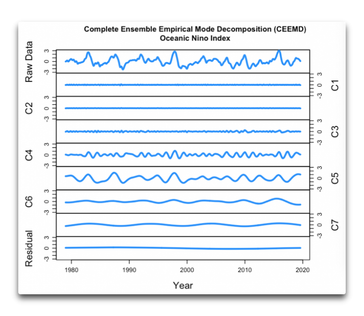
Figure 1. CEEMD analysis of the Oceanic Nino Index (ONI). Units are standard deviations of the underlying ONI signal.
From the top to the bottom, first you have the raw ONI data. Then you have the underlying signals, from the shortest period (highest frequency) signal group shown as empirical mode C1, to the longest period (lowest frequency) signal group shown as empirical mode C7. At the bottom you have the “Residual”, which is what’s left over after the removal of empirical mode signals C1 through C7. And if you add together all of those, C1 to C7 plus the residual … you reconstruct the original ONI signal exactly
As you can see, the strongest part of the signal is in empirical mode C5. This is the part of the signal with periods from about two to five years in length.
One of the most powerful uses of the CEEMD analysis is that it lets us see if two or more signals are closely related to each other. For example, Figure 2 below shows the empirical mode C5 for a variety of datasets. They include three temperature-based El Nino indices—the NINO34, ONI (Oceanic Nino Index), and MEI (Multivariate Enso Index).
Then there is one sea-level atmospheric pressure based El Nino index, the SOI (Southern Ocean Index). It is built around the difference in sea level pressure between Tahiti and Darwin, Australia.
There is one atmospheric temperature dataset, the UAH MSU satellite-based tropical lower troposphere temperature.
Finally, there are two total precipitable water (TPW) datasets. One is the tropical (23.5°N – 23.5°S) portion of the full ECMWF TPW dataset. The other is the RSS (Remote Sensing Systems) 20°N – 20°S ocean only TPW dataset. Here are the empirical mode 5 CEEMD results for all of them.
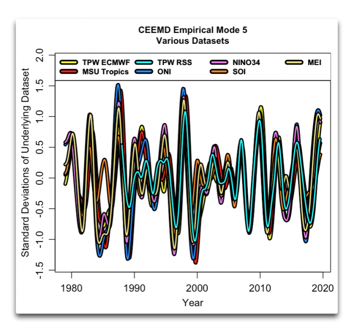
Figure 2. CEEMD empirical mode 5 results for a variety of datasets.
Interesting result, huh? You can see clearly that all of these datasets are moving in close harmony.
I got to thinking about this because in the comments to my last post, A Chain Of Effects, Matthew Sykes pointed out that the ECMWF total precipitable water (TPW) data was unlike the NVAP TPW data. To see who the outlier is, here are the CEEMD empirical mode 5 results for three different TPW results—the ECMWF, the RSS, and the NVAP total precipitable water datasets. The NVAP dataset starts in 1988, so I’ve started the comparison there.
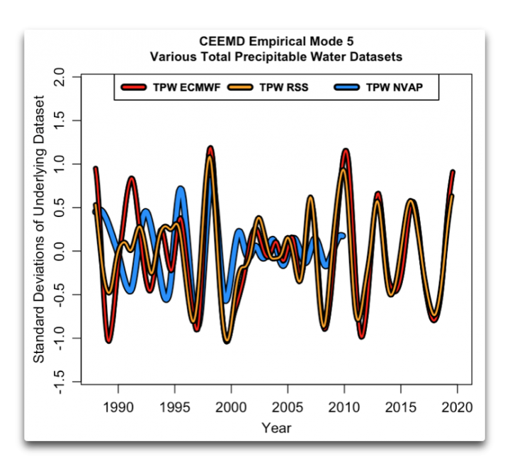
Figure 3. CEEMD empirical mode 5 results for three total precipitable water datasets.
From this, it seems clear that the NVAP dataset is the clear outlier. It goes into and out of sync with the other two, while the other two agree well throughout.
That answers the question that I came in on, as well as demonstrating the usefulness of the CEEMD analysis. And further deponent sayeth not.
Meanwhile, here on our Northern California coastal hillside with a tiny view of the ocean, we’re supposed to get big rain all week starting this morning (Tuesday) … fingers crossed. They say it will rain 2.7 inches (6.9 cm) today alone, which ain’t no ordinary rain, it’s a frog-strangler. But since we’ve only had about 40% of normal rain so far, I can only wish for a tropical downpour.
Best of this wondrous world to everyone,
w.
PS—I am happy to discuss and defend what I’ve said. However, I cannot defend or discuss what you think I said. As a result, I ask that when you comment you quote the exact words you are discussing so that we can all be clear on both who and what you are referring to.
CEEMS like a good idea.
My Mark 1 eyeball suggests the addition of a C8 1/2 sine periodicity c.22 years might even flatline the “residual.”
Willis, Thanks so much for this explanation of the CMEED process. I’ve been a bit puzzled and interested in your frequent use of it…it obviously is very powerful tool but I’d like to be able to fully understand it.
However as a mathematical drongo I still don’t quite get it. For example how are the C1-C7 categories chosen. You say they are ordered from the highest (C1) to lowest frequencies (C7) but how does one determine that there should be 7 categories not 27? Will each data set have a different number of C categories? Is the frequency range for each C class pre set or does that pop out of the data set somehow.
Could you please reply as if you’re talking to a 6 year old. Thanks.
Alastair, I spelled out the internal workings of the CEEMD process in my post linked above, “Noise Assisted Data Analysis“. Further details are in the paper “Ensemble Empirical Mode Decomposition: A Noise Assisted Data Analysis Method” linked in that post.
My best to you
w.
Thanks Willis, I’ll work through them and the comments tonight. If I still don’t get it (quite likely) I might get back to you if that’s OK.
Keep up the good work…we all appreciate it. Your posts add a lot of meat to WUWT rather than just political bickering and point scoring that some seem to love.
Much appreciated, Alastair. To be fair, it is totally counterintuitive to add noise to a dataset in order to understand it.
As always,
w.
From the Hilbert-Huange transform article in my other post (and I don’t pretend to fully understand this):
Mode mixing problemMode mixing problem happens during the EMD process. Straightforward implementation of sifting procedure produces mode mixing due to IMF mode rectification. Specific signal may not be separated into the same IMFs every time. This problem makes it hard to implement feature extraction, model training and pattern recognition since the feature is no longer fixed in one labeling index.
Ensemble empirical mode decomposition (EEMD)The proposed Ensemble Empirical Mode Decomposition is developed as follows:
The effects of the decomposition using the EEMD are that the added white noise series cancel each other, and the mean IMFs stays within the natural dyadic filter windows, significantly reducing the chance of mode mixing and preserving the dyadic property.
Looks like a form of Hilbert-Huang transform
https://en.wikipedia.org/wiki/Hilbert%E2%80%93Huang_transform#Definition
EMD is an iterative process to derive Intrinsic Mode Functions (IMFs) that are used to mathematically decompose non-stationary/non-linear data
EEMD somehow fixes the “mode mixing” problem of EMD by adding in white noise at the front end
However I’m not sure what the C=Complete for CEEMD means versus just plain EEMD
EEMD IMFs are by definition not generally mathematically complete (the E=empirical implies not complete, no?)
Maybe means completeness in this sense??…
https://en.wikipedia.org/wiki/Completeness_(order_theory)
whew way over my head though
CEEMD on the ONI just produces noise plots from a noisy signal. Tell me when the NEXT big El Nino is from those any of those modes and I might think it means something. Predicting the past is meaningless.
Looking at Figure 2, it seems to me that the primary mode for all of these datasets has a frequency of about 3.7 years. Interestingly, this is about 1/3 of a solar cycle.
Obviously, all of these data sets have the same primary driver, ocean temperatures. I would suspect that what controls, what seems to be a relatively stable frequency, is the mechanics of the circulation of ocean currents in the tropical Pacific.
When Paul Homewood posted an article on WUWT about Accumulated Cyclone Energy, on January 15, I found that there was a very good correlation between Global ACE and ENSO. I also found that the strongest peaks for Global ACE, like ENSO, occurred about 4 years after the solar cycle ramped up to its most active phase, i.e. what drives strong EL Ninos and active cyclone seasons is an interaction between ocean temperature cycles and the solar cycle.
So if you want to know when the next big El Nino will be, it is likely about 8 years off, ie. 2 1/2 ENSO cycles, and about 4 years or so after the current solar cycle ramps up to its most active phase.
Say what? CEEMD on the ONI reveals the underlying cycles just as it does with any signal. And if they are just “noise plots” as you claim, then why do they agree so well with the temperature and the TPW plots?
And no, it doesn’t predict the future, nor is it claimed to do so. Neither I nor anyone I know has made such a claim. You’re complaining that a table saw can’t dig post holes …
There are dozens of analysis methods out there that allow us to understand signals in greater depth … is Fourier Analysis “meaningless’ because it can’t predict the next big El Nino?
CEEMD good at what it’s good for. I use it, for example, to see if various climate signals have a sunspot-related component. And for that it’s far superior to Fourier Analysis … but that doesn’t make Fourier Analysis “meaningless” either. You need to pick the right tool for each job.
Sorry, amigo, usually your comments are meaty and full of interesting ideas, but as far as I can see this one totally misses the point of the whole post.
My best to you in any case,
w.
CEEMD isn’t necessarily used to predict future cycles. The prior cycles may have random length or amplitude. CEEMD is extremely useful for comparing plots of different variables to see if “two or more signals are closely related to each other“, as Willis explained and demonstrated. The only time it could “predict the future” is if the cycles were of predictable length. It is an extremely useful technique when dealing with seemingly random or chaotic data.
Just a Teuchter’s view here. This method is good at eliminating what it isn’t and possibly what it is that causes something to happen. But until we have something predictable as the cause we can’t predict anything. But if more than one unpredictable is involved then it’s down to a guess. As all things in nature are inherently unpredictable to then we’re talking long range weather forecasting.
Seems like a variant of the multi-resolution decomposition technique using wavelet basis functions (many different options of basis sets). One nice thing in this approach is the ability to decompose the data into the different 2^N levels and examine each level for the presence of stochastic noise. Then one can reassemble the data with the pure noise levels removed. This has been used for 20 year in oil field seismology. This is a great approach! Good work.
“They say it will rain 2.7 inches (6.9 cm) today alone, which ain’t no ordinary rain, it’s a frog-strangler.”
That’s a handy little scud, which I would have thought typical of a tropical thunderstorm.
I know this is way off the main topic, but the little asides such as “what counts as heavy rain in different areas” can be quite interesting as well.
This is extremely interesting. Most of the plots in figure 2 are so in line that my “suspicion” radar turns on…when something looks too good to be true…Makes me wonder if the data does not rely on each other somehow when they “adjust” it. That or it’s just really related.
I note there are two large discrepancies. 1) SOI around 1985 is inverted from the other data sets – given it’s behavior after that it makes me wonder why. 2) TPW RSS appears really out of phase in the early 1990’s. Again, I wonder why that is so? Did they replacee a satellite sensor in or around 1996?
Wouldn’t it be cool if you have found a new way to check for faulty or badly calibrated data senors.
This to me is one of the strongest points of CEEMD, which is that it can show where a signal changes.
w.
Early 1990’s yes, but that is just before 1985, think volcanoes.
Looks like W gets his wish
Thank you, Willis, for this excellent explanation and example of CEEMD. I’ve tried it myself on the UAH TEMP data set in R Studio to locate trends, but with very little understanding. This is extremely helpful, and the comparison with TPW is fascinating. Bookmarking this.
Looks like Wavelet analysis under a different name.
Willis, sorry to bother you but I was wondering if you could help me with CEEMD. I wanted to use it on some other data but I thought I’d try to replicate what you did with the sunspot data just to make sure I could get reasonable answers. I tried replicating your sunspot graphs but I don’t see how you were generating the formatting. Was they part of the hht package, another package or did you roll your own with ggplot? The periodograms that you show are in the time domain(1/f) rather than frequency but all I managed to find in hht was frequency in one graph rather than stacked like yours.
Another question I had was what you were using for the white noise parameter noise.amp since there’s no default and the doc for hht doesn’t give any hints. My results “look” close to yours but there are some differences. I am using the latest data which has six more years than the one you did in 2014 so I don’t know if that has an effect either.
This is the code I’m using
cresults = CEEMD(sig=spnum.std,tt=ts(spyear),noise.amp = 1, trials=100);
Thanks for any help
Barry
Bear, as is my usual habit, I’ve written R functions that make it easier to use and interpret CEEMD. And as is also common on my planet, they depend on other functions I’ve written, and on down the line. Hang on, this will take me a while … OK, I’ve put my CEEMD function and what I think are the other related functions in a zipped file here. It contains my main R functions file called “Willis Functions” which has a host of other functions including some needed for the CEEMD functions, you’re welcome to use anything you find.
Let me know if any functions are missing and I’ll send them along.
My best to you,
w.
Thank you so much.
Barry
“Deponement”? You made me look up a werd . . . Moncton makes me look up many more.