Guest Post by Willis Eschenbach
I got to thinking about the lack of progress in estimating the “equilibrium climate sensitivity”, known as ECS. The ECS measures how much the temperature changes when the top-of-atmosphere forcing changes, in about a thousand years after all the changes have equilibrated. The ECS is measured in degrees C per doubling of CO2 (°C / 2xCO2).
Knutti et al. 2017 offers us an interesting look at the range of historical answers to this question. From the abstract:
Equilibrium climate sensitivity characterizes the Earth’s long-term global temperature response to increased atmospheric CO2 concentration. It has reached almost iconic status as the single number that describes how severe climate change will be. The consensus on the ‘likely’ range for climate sensitivity of 1.5 °C to 4.5 °C today is the same as given by Jule Charney in 1979, but now it is based on quantitative evidence from across the climate system and throughout climate history.
This “climate sensitivity”, often represented by the Greek letter lambda (λ), is claimed to be a constant that relates changes in downwelling radiation (called “forcing”) to changes in global surface temperature. The relationship is claimed to be:
Change in temperature is equal to climate sensitivity times the change in downwelling radiation.
Or written in that curious language called “math” it is
∆T = λ ∆F Equation 1 (and only)
where T is surface temperature, F is downwelling radiative forcing, λ is climate sensitivity, and ∆ means “change in”
I call this the “canonical equation” of modern climate science. I discuss the derivation of this equation here. And according to that canonical equation, depending on the value of the climate sensitivity, a doubling of CO2 could make either a large or small change in surface temperature. Which is why it the sensitivity is “iconic”.
Now, I describe myself as a climate heretic, rather than a skeptic. A heretic is someone who does not believe orthodox doctrine. Me, I question that underlying equation. I do not think that even over the long term the change in temperature is equal to a constant time the change in downwelling radiation.
My simplest objection to this idea is that evidence shows that the climate sensitivity is not a constant. Instead, it is a function inter alia of the surface temperature. I will return to this idea in a bit. First, let me quote a bit more from the Knutti paper on historical estimates of climate sensitivity:
The climate system response to changes in the Earth’s radiative balance depends fundamentally on the timescale considered. The initial transient response over several decades is characterized by the transient climate response (TCR), defined as the global mean surface warming at the time of doubling of CO2 in an idealized 1% yr–1 CO2 increase experiment, but is more generally quantifying warming in response to a changing forcing prior to the deep ocean being in equilibrium with the forcing …
By contrast [to Transient Climate Response TCR], the equilibrium climate sensitivity (ECS) is defined as the warming response to doubling CO2 in the atmosphere relative to pre-industrial climate, after the climate reached its new equilibrium, taking into account changes in water vapour, lapse rate, clouds and surface albedo.
It takes thousands of years for the ocean to reach a new equilibrium. By that time, long-term Earth system feedbacks — such as changes in ice sheets and vegetation, and the feedbacks between climate and biogeochemical cycles — will further affect climate, but such feedbacks are not included in ECS because they are fixed in these model simulations.
Despite not directly predicting actual warming, ECS has become an almost iconic number to quantify the seriousness of anthropogenic warming. This is a consequence of its historical legacy, the simplicity of its definition, its apparently convenient relation to radiative forcing, and because many impacts to first order scale with global mean surface temperature.
The estimated range of ECS has not changed much despite massive research efforts. The IPCC assessed that it is ‘likely’ to be in the range of 1.5 °C to 4.5 °C (Figs 2 and 3), which is the same range given by Charney in 1979. The question is legitimate: have we made no progress on estimating climate sensitivity?
Here’s what the results show. There has been no advance, no increase in accuracy, no reduced uncertainty, in ECS estimates over the forty years since Carney in 1979. Let’s take a look at the actual estimates.
The Knutti paper divides the results up based on the type of underlying data upon which they were determined, viz: “Theory & Reviews”, “Observations”, “Paleoclimate”, “Constrained by Climatology”, and “GCMs” (global climate models). Some of the 145 estimates only contained a range, like say 1.5 to 4.5. In that case, for the purposes of Figure 1 I’ve taken the mean of the range as the point value of their estimate.

Next, I looked at the 124 estimates which included a range for the data. Some of these are 95% confidence intervals; some are reported as one standard deviation; others are a raw range of a group of results. I have converted all of these to a common standard, the 95% confidence interval. Figure 2 shows the maxima and the minima of these ranges. I have highlighted the results from the five IPCC Assessment Reports, as well as the Charney estimate.

The Charney / IPCC estimates for the range of the ECS values are constant from 1979 to 1995, at 1.5°C to 4.5°C for a doubling of CO2. In the Third Assessment Report (TAR) in 2001 the range gets smaller, and in the Fourth Assessment Report (AR4) in 2007 the range got smaller still.
But in the most recent Fifth Assessment Report (AR5), we’re back to the original ECS range where we started, at 1.5 to 4.5°C / 2xCO2.
In fact, far from the uncertainty decreasing over time, the tops of the uncertainty ranges have been increasing over time (red/black line). And at the same time, the bottoms of the uncertainty ranges have been decreasing over time (yellow/black line). So things are getting worse. As you can see, over time the range of the uncertainty of the ECS estimates has steadily increased.
Looking At The Shorter Term Changes.
Pondering all of this, I got to thinking about a related matter. The charts above show equilibrium climate sensitivity (ECS), the response to a CO2 increase after a thousand years or so. There is also the “transient climate response” (TCR) mentioned above. Here’s the definition of the TCR, from the IPCC:
Transient Climate Response (TCR)
TCR is defined as the average global temperature change that would occur if the atmospheric CO2 concentration were increased at 1% per year (compounded) until CO2 doubles at year 70. The TCR is measured in simulations as the average global temperature in a 20-year window centered at year 70 (i.e. years 60 to 80).
The transient climate response (TCR) tends to be about 70% of the equilibrium climate sensitivity (ECS).
However, this time I wanted to look at an even shorter-term measure, the “immediate climate response” (ICR). The ICR is what happens immediately when radiation is increased. Bear in mind that the effect of radiation is immediate—as soon as the radiation is absorbed, the temperature of whatever absorbed the radiation goes up.
Now, a while back Ramanathan proposed a way to actually measure the strength of the atmospheric greenhouse effect. He pointed out that if you take the upwelling surface longwave radiation, and you subtract upwelling longwave radiation measured at the top of the atmosphere (TOA), the difference between the two is the amount of upwelling surface longwave that is being absorbed by the greenhouse gases (GHGs) in the atmosphere. It is this net absorbed radiation which is then radiated back down towards the planetary surface. Figure 3 shows the average strength of the atmospheric greenhouse effect.

The main forces influencing the variation in downwelling radiation are clouds and water vapor. We know this because the non-condensing greenhouse gases (CO2, methane, etc) are generally well-mixed. Clouds are responsible for about 38 W/m2 of the downwelling LW radiation, CO2 is responsible for on the order of another twenty or thirty W/m2 or so, and the other ~ hundred watts/m2 or so are from water vapor.
So to return to the question of immediate climate response … how much does the monthly average surface temperature change when there are changes in the monthly average downwelling longwave radiation shown in Figure 3? This is the immediate climate response (ICR) I mentioned above. Figure 4 below shows how much the temperature changes immediately with respect to changes in downwelling GHG radiation (also called “GHG forcing”).

There are some interesting things to be found in Figure 4. First, as you might imagine, the ocean warms much less on average than the land when downwelling radiation increases. However, it was not for the reason I first assumed. I figured that the reason was the difference in thermal mass between the ocean and the land. However, if you look at the tropical areas you’ll see that the changes on land are very much like those in the ocean.
Instead of thermal mass, the difference in land and sea appears to be related to land and sea snow and ice. These are generally the green-colored areas in Figure 4 above. When ice melts either on land or sea, much less sunlight is reflected back to space from the surface. This positive feedback increases the thermal response to increased forcing.
Next, you can see evidence for the long-discussed claim that if CO2 increases, there will be more warming near the poles than in the tropics. The colder areas of the planet warm the most from an increase in downwelling LW radiation. On the other hand, the tropics barely warm at all with increasing downwelling radiation.
Seeing the cold areas warming more than the warm areas led me to graph the temperature increase per additional 3.7 W/m2 versus the average temperature in each gridcell, as seen in Figure 5 below.

The yellow/black line is the amount that we’d expect the temperature to rise (using the Stefan-Boltzmann equation) if the downwelling radiation goes up by 3.7W/m2 and there is no feedback. This graph reveals some very interesting things.
First, at the cold end, things warm faster than expected. As mentioned above, I would suggest that at least in part this is the result of the positive albedo feedback from the melting of land and sea ice.
There is support for this interpretation when we note that the right-hand part of Figure 5 that is above freezing is very different from the left-hand part that is below freezing. Above freezing, the temperature rise per additional radiation is much smaller than below freezing.
It is also almost entirely below the theoretical response. The average immediate climate response (ICR) of all of the unfrozen parts of the planet is a warming of only 0.2°C per 3.7 W/m2.
Discussion
We’re left with a question: why it is that forty years after the Charney report, there has been no progress in reducing the uncertainty in the estimate of the equilibrium climate sensitivity?
I hold that the reason is that the canonical equation is not an accurate representation of reality … and it’s hard to get the right answer when you’re asking the wrong question.
From above, here’s the canonical equation once again:
This “climate sensitivity”, often represented by the Greek letter lambda (λ), is claimed to be a constant that relates changes in downwelling radiation (called “forcing”) to changes in global surface temperature. The relationship is claimed to be:
Change in temperature is equal to climate sensitivity times the change in downwelling radiation.
Or written in that curious language called “math” it is
∆T = λ ∆F Equation 1 (and only)
where T is surface temperature, F is downwelling radiative forcing, λ is climate sensitivity, and ∆ means “change in”
I hold that the error in that equation is the idea that lambda, the climate sensitivity, is a constant. Nor is there any a priori reason to assume it is constant.
Finally, it is worth noting that in areas above freezing, the immediate change in temperature per doubling of CO2 is far below the amount expected from just the known Stefan-Boltzmann relationship between radiation and temperature (yellow/black line in Figure 5). And in the areas below freezing, it is well above the amount expected.
And this means that just as the areas below freezing are showing clear and strong positive feedback, the areas above freezing are showing clear and strong negative feedback.
Best Christmas/Hannukah/Kwanzaa/Whateverfloatsyourboat wishes to all,
w.
AS USUAL, I ask that when you comment you quote the exact words you are discussing, so we can all be certain what you are referring to.
A few thoughts…
1. Prof. Will Happer has found evidence that that 3.7±0.4 W/m² estimate for the average increase in ground level irradiance, before feedbacks, is overestimated by about 40% [also Happer 2014]. So:
(3.7 ±0.4) / 1.4 = 2.64 ±0.29 W/m² / doubling.
That seems to have been confirmed by the measurements of reported in Feldman et al 2015. They measuring downwelling LW IR spectrum directly, over a ten year period, during which average atmospheric CO2 levels rose 22 ppmv.
A 22 ppmv increase (+5.953% from 369.55 ppmv in 2000) in atmospheric CO2 level resulted in 0.2 ±0.06 W/m² increase in downwelling 15 µm IR from CO2. (5.953% is about 1/12 of a doubling.)
(1/log2(1.0593)) × 0.2 W/m² = 2.41 W/m² (central value)
(1/log2(1.0593)) × (0.2 – 0.06 W/m²) = 1.68 W/m² (low end)
(1/log2(1.0593)) × (0.2 + 0.06 W/m²) = 3.13 W/m² (high end)
So, we find that CO2 forcing is 2.41 ±0.73 W/m² / doubling, which is consistent with Happer’s result, and inconsistent with the commonly heard 3.7 ±0.4 W/m² estimate.
2. AR5 Table 9.5 gives the average ECS in the CMIP5 models as 3.2 ±1.3 °C/doubling (rather than the “Mean 3.3°C” shown in Fig. 1 from Knutti), using a 90% (instead of 95%) confidence interval:
pdf: https://sealevel.info/AR5_Table_9.5_p.818.pdf
source: http://www.ipcc.ch/pdf/assessment-report/ar5/wg1/WG1AR5_Chapter09_FINAL.pdf#page=78
spreadsheet: https://sealevel.info/AR5_Table_9.5_p.818.pdf (and I added one additional column)
3. I agree with your “heresy,” Willis, that climate sensitivity is not constant, but I don’t think that’s really very heretical. It’s pretty well understood that Global Warming disproportionately warms high northern latitudes. Climate activists call it “Arctic amplification,” and they all think that brutal northern climates becoming slightly less harsh is a terrible thing — which, IMO, is proof of insanity.
Arrhenius enthusiastically predicted it, and, sure enough, we’re enjoying “more equable and better climates, especially as regards the colder regions of the earth… [and] much more abundant crops… for the benefit of… mankind.”
In any event, we can finesse the objection by simply inserting the word “average” into the “sensitivity” definitions. E.g.,
TCR n. The effect on the Earth’s average global near-surface air temperature after seventy years, of increasing the atmospheric CO2 level by 1% per year (a rate of increase which would double the CO2 level in seventy years).
4. The most straightforward and obvious way of estimating climate sensitivity to a doubling of CO2 is by examining the result of the “experiment” which we’ve performed on the Earth’s climate, by raising the atmospheric CO2 level from about 311 ppmv in 1950 (or from 285 ppmv in 1850) to about 412 ppmv now. We simply examine what happened to temperatures when the atmospheric CO2 level was raised by 32% (or 45%), and extrapolate from those observations.
However, there are a few pitfalls with that approach. For one thing, natural global temperatures variations due to ENSO can be larger than the “signal” we’re looking for, especially for the earlier part of the record, when CO2 was rising very slowly, so it is important that we choose an analysis interval which avoids those distortions. For another thing, it would be a mistake to assume that all of the warming which the Earth has experienced since pre-industrial conditions was due to anthropogenic CO2, because much of that warming occurred when CO2 levels were still very low, and because we know of other factors which must have contributed to warming, such as rising levels of other GHGs, and probably aerosol/particulate pollution abatement.
I did that exercise, using the period 1960-2014, which encompasses most of the period of rapid CO2 level increases, while avoiding distortions from major ENSO spikes. I calculated TCR two ways:
1. Assuming 100% of the warming trend was anthropogenic (and 75% of that was from CO2). That yielded a TCR of 1.41°C per doubling of CO2.
2. Assuming 57% of the warming was anthropogenic. That yielded a TCR of 0.81 °C per doubling of CO2.
Details here:
https://sealevel.info/sensitivity.html
(Sorry for the botched a </a> tag.)
Does it not follow from the T>4 relationship, that it is far more difficult to warm the warmer equitorial regions of the planet than it is to warm the cool polar regions of the planet?
Given that relationship is it not inevitable that we will see the cool polar regions warming faster and by larger increments than the warm equitorial regions of the planet?
More difficult, yes, but I wouldn’t call it “far more” difficult.
In Guayaquil, Ecuador the average temperature is about 26°C.
At Prudhoe Bay, Alaska, the average temperature is -11°C.
The question is, how much more radiative emission do you get from one degree of warming at Guayaquil, compared to one degree of warming at Prudhoe Bay?
The S-B (T^4) rule applies to absolute temperatures. Absolute (Kelvin) temperature is Celsius temperature + 273.15.
Guayaquil: 26°C = 299.15K
Prudhoe Bay: -11°C = 262.15K
So, let’s compare the effect on radiative emissions of one degree of warming in each of those two places:
(300.15^4 – 299.15^4) / (263.15^4 – 262.15^4) = 1.485
So it’s 48.5% more difficult to raise temperature by a given increment in Equador than northern Alaska.
Or, rather, that’s what the difference would be, if radiation were the only way heat is lost by the surface. But, of course, it’s not. It’s not even the most important way. The water cycle is much more important, in most places.
Guayaquil and Prudhoe Bay are both harbors, so they’re at the same altitude, and both are next tot he ocean. But I’ll bet raising the air temperature from 26°C to 27°C would affect the evaporation rate at Guayaquil a lot more than raising the air temperature from -11°C to -10°C would affect the evaporation and sublimation rates at Prudhoe Bay.
s/their at/they’re at/
Sheesh, I can’t believe I wrote THAT. Must be bedtime.
Fixed. I hate typos and the like.
w.
Gracias, amigo!
I’m having trouble following the logic.
You say, “The ICR is what happens immediately when radiation is increased. Bear in mind that the effect of radiation is immediate—as soon as the radiation is absorbed, the temperature of whatever absorbed the radiation goes up.”
What do you mean by “immediately”? It seems to me that when you’re discussing absorption as opposed to emission some time duration must be involved for a given power to raise temperature by a given amount. Yet your only quantities are changes in powerdensity (W/m^2) and temperature; no time duration, at least not explicitly.
(In contrast, I suppose, emitted radiation changes immediately in response to a black body’s temperature.)
I cannot think of anything more tedious and futile than seeking this holy grail through mathematical calculation.
Please establish for me a constant for wing-tip velocity of a butterfly’s wing vs lift, in the natural environment.
How can so many intelligent people be blinded by their computer screens?
Willis:
Thought provoking as ever, Willis.
I know where TOA measurements come from but it is unclear from your presentation what you are using for the “surface” upwards LWIR. Could you explain where that comes from?
The one thing that strikes me about fig 5 is the step jump from about 0.2 K/2xCO2 to about 1K/2xCO2 which happens around zero deg C. What is the difference either side of that : the presence / absence of evaporation.
As you started pointing out years ago in relation to the tropics, it evaporation/advection/precipitation which controls tropical climate, not CO2.
The ramping as it gets much colder than zero points to the other key factor being absolute humidty. Air that cold has very little water vapour content and no open water.
As most here already know it is H2O which controls climate.
thx.
—————————-
Pangburn
Shows that temperature change over the last 170 years is due to 3 things: 1) cycling of the ocean temperature, 2) sun variations and 3) moisture in the air. There is no significant dependence of temperature on CO2.
https://globalclimatedrivers2.blogspot.com/
—————————–
Princeton researchers have uncovered new rules governing how objects absorb and emit light, fine-tuning scientists’ control over light and boosting research into next-generation solar and optical devices.
The discovery solves a longstanding problem of scale, where light’s behavior when interacting with tiny objects violates well-established physical constraints observed at larger scales.
described in https://phys.org/news/2019-12-illuminate-absorb-emit.html
Being a nuclear engineer (retired) I have always questioned why blackbody rules were applied to individual atoms floating in the atmosphere separated from each other, and these distances increase with height in the atmosphere.
There is also a great article on Space dot com https://www.space.com/ionosphere-science-roundup.html
That at an altitude of roughly 50 to 400 miles (80 to 645 kilometers), is full of strange physical phenomena that scientists are only beginning to understand. In the ionosphere, charged particles released by the sun interact with gases at the top of Earth’s atmosphere in intriguing ways.
“For one, it showed scientists that when a solar storm hits Earth, atomic oxygen becomes more common at low latitudes and rarer at high latitudes. At the same time, molecular nitrogen prevalence does the opposite, decreasing at low latitudes and increasing at high latitudes.”
This article tells me that there are still BIG questions about what happens to our atmosphere and just how energy moves in the atmosphere.
@ur momisugly Willis is Fig. 3 just showing that downwelling radiation is a constant fraction of the upwelling?
Jit December 26, 2019 at 1:50 pm
No. It’s showing the actual downwelling radiation, calculated as upwelling surface LW minus upwelling LW at the top of atmosphere, as described in the post.
Regards,
w.
A poorly phrased question! How about this: is the downwelling a constant fraction of the upwelling…?
No, it varies, both in space and time.
w.
Fig. 3 and 4: The colder the location (Arctic and especially Antarctic) the higher the warming effect. The colder the location, the less water vapor (and clouds) are present in the air. At very low concentrations each added water vapor molecule gives a very high temperature response. High and dry and super cold Antarctica, nearly void of water vapor gives the highest response: each added water vapor molecule counts.
Nobody lives in Antarctica there where we find the highest response. Temperatures still remain very very low. In the Arctic we don’t find many people either.
Fig. 5: interesting the small blue flag representing 71% of the surface of the Earth, the oceans. Nearly nothing happens. Long wave radiation cannot penetrate water surfaces deeply, just 0.01 mm or so. If the energy remains in the upper upper layer of the ocean (conduction by water is low) the extra energy probably leads to extra evaporation and some loss of sensible energy and both are cooling the surface.
ECS is nothing more than a pitiful attempt by those who don’t understand real-world thermodynamics to characterize climate-scale planetary temperature variations on the cheap.
… worse than astrology.
I think that trying to determine a single number (lambda) to predict future global warming resulting from a doubling of CO2 is an over-simplification of the problem. The approach is probably only valid for deserts (both cold and hot). That is, the inhibition of the loss of energy to space is a combination of the combined effects of water vapor and CO2 (actually all so-called Greenhouse Gases).
It is generally acknowledged that the Arctic is warming at a rate two or three times the average for the globe. I think that the most probable explanation is that there is negligible water vapor over the Arctic, so the only thing affecting absorption is increasing CO2. I suspect that one would find that the Sahara Desert is similarly warming at night more rapidly than the rest of the Earth.
However, I don’t know if anyone is looking because a warming Sahara won’t melt any ice or cause sea level to rise. My conjecture is that all climate zones will have a unique lambda, which may change over time. However, most of the world has substantial water vapor, which varies with the season and temperatures, but isn’t increasing as rapidly as CO2. Thus, focusing on CO2 in the definition of lambda implicitly uses CO2 as a proxy for all Greenhous Gases, including water vapor.
Thus, the proper approach to the problem would be to determine the unique Greenhouse Gas lambda for all Köppen Climate Zones, and do an area-weighting to determine a global average. It would be instructive to see what the predicted warming would then be for just the climate zones where most people live. As it is, it is naively assumed that whatever the calculated CO2 lambda is, it correctly predicts what people who live in humid areas can expect. Probably, the warming in the tropics and mid-latitudes will be considerably less than is predicted by the consensus CO2 lambda.
I’m reminded that after the Three Mile Island release of radioactivity, the government assured everyone that the average exposure to inhabitants in a circular area around the reactor, of a given diameter, was well below the threshold for concern. However, they failed to acknowledge that the radioactive releases were concentrated in plumes downwind of the reactor. Averages can be quite misleading!
The problem lies not only in the variability of lambda, as simplistically defined here, but also in the failure to specify any physically meaningful spatio-temporal scale for “climatic” temperature variations. Furthermore, the driver of surface temperatures on any scale is by no means simply “downwelling radiative forcing,” but involves the non-radiative mechanisms of evaporation and convection.
In the real world, heat transfer by moist convection from the surface to atmosphere exceeds all other mechanisms combined. That’s why attempts to find the “true” value of lambda invariably produce values so widely scattered as to render any claim of having established a critical physical ratio totally risible.
The IPCC has been systematically rejecting all rationale to support ideas that the climate sensitivity of CO2 is actually significantly less than the range of guesses that they have been publishing. I believe that the reason for this is politics. If the IPCC came out and declared that the the climate sensitivity is significantly less than previously thought, they would expect that their funding would be reduced significantly. Initial radiametric calculations came up with a value for the climate sensitivity of CO2, not including feedbacks, of 1.2 degrees C. Work by a group of scientists looking at temperature data from roughly 1850 to a few years ago showed that if all the warming were caused by CO2, the climate sensitivity of CO2 could not be more than 1.2 degrees C. A researcher from Japan pointed out the the original calculations neglected to take into consideration that a doubling of CO2 will cause a slight decrease in the dry lapse rate in the troposphere which would decrease the climate sensitivity of CO2 by more than a factor of 20 yielding a climate sensitivity of CO2 before feedbacks of less than .06 degrees C which is trivial. Then there is the issue of H2O feedback. Proponents of the AGW conjecture tend to ignore that fact that besides being the primary greenhouse gas, if you believe in such things, H2O is a primary coolant in the Earth’s atmosphere. The over all cooling effects of H2O are evidenced by the fact that the wet lapse rate is significantly less that the dry lapse rate. So hence instead of providing positive feedback, H2O provides negative feedback and retards any warming that CO2 might provide. Negative feedback systems are inherently stable as has been the Earth’s climate for at least the past 500 million years, enough for life to evolve. We are here. So there is rationale that the actual climate sensitivity of CO2 may be somewhere between .06 and 0.0 degrees C.
The basic issue is that there is no such thing as a climate sensitivity to CO2 or any other so called ‘greenhouse gas’. Radiative forcing can politely be described as climate theology – how does a change in the atmospheric concentration of CO2 change the number of angels that may dance on the head of a climate pin? The climate equilibrium assumption was used by Arrhenius in his 1896 estimate of global warming. In this paper he traced the concept back to Pouillet in 1838. Speculation that changes in atmospheric CO2 concentration could somehow cause an Ice Age started with John Tyndall in 1863. To get to the bottom of the radiative forcing nonsense it is necessary to go back to Fourier in 1827 and start over with the real physics of the surface energy transfer.
The essential part that almost everyone seems to have missed in this paper is the time delay or phase shift between the solar flux and the surface temperature response. The daily phase shift in MSAT can reach 2 hours and the seasonal phase shift can reach 6 to 8 weeks. This is clear evidence for non-equilibrium thermal storage. The same kind of non-equilibrium phase shift on different time and energy scales occurs with electrical energy storage in capacitors and inductors in AC circuits – low pass filters, tank circuits etc.
The equilibrium average climate assumption was used by Manabe and Wetherald (M&W) in their 1967 climate modeling paper. They abandoned physical reality and created global warming as a mathematical artifact of their input modeling assumptions. The rest of the climate modelers followed like lemmings jumping off a cliff. In the 1979 Charney report, no-one looked at the underlying assumptions. The radiative transfer results were reasonable –for the total long wave IR (LWIR) flux at the top and bottom atmosphere – and the mathematical derivation of the flux balance equations was correct. The increase in surface temperature was the a-priori expected result. Radiative forcing and the invalid equilibrium flux balance equations were discussed by Ramanathan and Coakley in 1978. The prescribed mathematical ritual of radiative forcing in climate models was described by Hansen et al in 1981. They also introduced a fraudulent ‘slab’ ocean model and did a bait and switch from surface to weather station temperatures. The LWIR flux interacts with the surface, not the weather station thermometer at eye level above the ground. Radiative forcing is still an integral part of IPCC climate models [IPCC, 2013]. Physical reality has been abandoned in favor of mathematical simplicity. Among other things, M&W threw out the Second Law of Thermodynamics along with at least 4 other Laws of Physics. The underlying requirement for climate stability is that the absorbed solar heat be dissipated by the surface. This requires a time dependent thermal and or humidity gradient at the surface.
The starting point for any realistic climate system is that the upward LWIR flux from the top of the atmosphere does not define an equilibrium average temperature of 255 K. Instead it is the cumulative cooling flux emitted from multiple levels down through the atmosphere. The upward emission from each level is then attenuated by the LWIR absorption/emission along the upward path to space [Feldman et al, 2008]. Another fundamental error in the radiative forcing argument is the failure to consider the molecular line width effects. Part of this was due to the band model simplifications that are still used in the climate models to speed up the calculations. The IR flux through the atmosphere consists of absorption and emission from many thousands of overlapping molecular lines, mainly from CO2 and water vapor [Rothman et al, 2005]. As the temperature and pressure decrease with altitude, these lines become narrower and transmission ‘gaps’ open up between the lines. This produces a gradual transition from absorption/emission to a free photon flux to space.
The radiative forcing argument has also obscured the fact that the heat lost to space is replaced by convection, not LWIR radiation. The troposphere is an open cycle heat engine that transports heat from the surface by moist convection. It is stored in the troposphere as gravitational potential energy. As a high altitude air parcel cools by LWIR emission, it contracts and sinks back down through the troposphere. The upward LWIR flux to space is decoupled from the surface by the linewidth effects. The downward LWR flux from the upper troposphere cannot reach the surface and cause any kind of change in the surface temperature. Almost all of the downward LWIR flux reaching the surface originated from within the first 2 km layer of the troposphere and about half of this comes from the first 100 m layer.
Near the surface, the lines in the main bands for CO2 and water vapor are sufficiently broadened that they merge into a continuum. There is an atmospheric transmission window in the 8 to 12 micron spectral region that allows part of the surface LWIR flux to escape directly to space. The magnitude of this transmitted cooling flux varies with cloud cover and humidity. The downward LWIR flux to the surface from the broad molecular emission bands provides an LWIR exchange energy that ‘blocks’ the upward LWIR flux from the surface. Photons are exchanged without any net heat transfer. In order for the surface cool, it must heat up until the excess absorbed solar heat is removed by moist convection. This is the real cause of the so called ‘greenhouse effect’. It requires the application of the Second Law of Thermodynamics to the surface exchange energy. There is no equilibrium average climate so there can be no average ‘greenhouse effect temperature’ of 33 K. Instead, the greenhouse effect is just the downward LWIR flux from the lower troposphere to the surface. It can be defined as the downward flux or as an ‘opacity factor’ [Rorsch, 2019]. This is the ratio of the downward flux to the total blackbody surface emission.
The surface temperature has to be calculated at the surface using the surface flux balance. The change in local surface temperature is determined by the change in heat content or enthalpy of the local surface thermal reservoir divided by the specific heat [Clark, 2013a, b]. The LWIR flux cannot be separated from the other flux terms and analyzed independently. The land and ocean surface behave differently and have to be considered separately.
Over land, the various flux terms interact with a thin surface layer. During the day, the surface heating produces a thermal gradient both with the cooler air layer above and the subsurface layers below. The surface-air gradient drives the convection or sensible heat flux. The subsurface thermal gradient conducts heat into the first 0.5 to 2 meter layer of the ground. Later in the day this thermal gradient reverses and the stored heat is released back into the troposphere. The thermal gradients are reduced by evaporation if the land surface is moist. An important consideration in setting the land surface temperature is the night time convection transition temperature at which the surface and surface air temperatures equalize. Convection then essentially stops and the surface continues to cool more slowly by net LWIR emission. This convection transition temperature is reset each day by the local weather conditions.
The ocean surface is almost transparent to the solar flux. Approximately 90% of the solar flux is absorbed within the first 10 m ocean layer. The surface-air temperature gradient is quite small, usually less than 2 K. The excess absorbed solar heat is removed through a combination of net LWIR emission and wind driven evaporation. The penetration depth of the LWIR flux into the ocean surface is 100 µm or less and the evaporation involves the removal of water molecules from a thin surface layer [Hale and Querry, 1972]. These two processes combine to produce cooler water at the surface that sinks and is replaced by warmer water from below. This is a Rayleigh-Benard convection process, not simple diffusion. There are distinct columns of water moving in opposite directions. The upwelling warmer water allows the wind driven ocean evaporation to continue at night. As the cooler water sinks, it carries with it the surface momentum or linear motion produced by the wind coupling at the surface. This establishes the subsurface ocean gyre currents. Outside of the tropics there is a seasonal phase shift that may reach 6 to 8 weeks.
This phase shift can only occur with ocean solar heating. The heat capacity of the land thermal reservoir is too small to produce this effect. In many parts of the world, the prevailing weather systems are formed over the ocean. The temperature changes related to the ocean surface are stored by the weather system as the bulk surface air temperature and this information can be transported over very long distances. Such ocean related phase shifts can be found in the daily climate data for weather stations in places like Sioux Falls SD.
Over the oceans, the wind driven evaporation can never exactly balance the solar heating. This produces the ocean oscillations such as the ENSO, PDO and AMO. These surface temperature changes are incorporated into the various weather systems and can be seen in the long term climate data, particularly the minimum MSAT. The whole global warming scam is based on nothing more than the last AMO warming cycle coupled into the weather station data [Akasofu, 2010].
A fundamental failure of the radiative forcing argument is the lack of any error analysis. Over the last 200 years, the atmospheric CO2 concentration has increased by a little over 120 ppm. This has produced an increase in the downward LWIR flux at the surface of about 2 W m-2 [Harde, 2017]. Over the oceans this is coupled into the first 100 micron layer of the ocean surface. Here it is fully coupled to the wind driven evaporation. Using long term ocean evaporation data from Yu et al, 2008, an approximate estimate of the evaporation rate within the ±30 degree latitude region is 15 Watts per square meter for each change in wind speed of 1 meter per second. This means that the radiative forcing from an increase of 120 ppm in the CO2 concentration amounts to a change in wind speed of about 13 CENTIMETERS per second. This is at least two orders of magnitude below the normal variation in ocean wind speed. Similarly, a reasonable estimate of the bulk convection coefficient for dry land is 20 Watts per square meter per degree C difference between surface and air temperature. Here a 2 W m-2 change in convection requires a change of 0.1 C in the surface air thermal gradient. Once the physics of the time dependent surface energy transfer is restored, global warming and radiative forcing disappear into the realm of computerized climate fiction.
The topic of radiative forcing was recently reviewed in detail by Ramaswamy et al [2019] as part of the American Meteorological Society monographs series. This review provides a good start for a scientific and criminal fraud investigation into the climate modeling fraud. To begin, the scientific community should demand that this particular monograph be retracted and all further work on equilibrium climate modeling be stopped. Any climate model that uses radiative forcing is by definition invalid. There is no need to try and validate the computer code of any equilibrium climate model. The use of radiative forcing alone is sufficient to render the results totally useless. These modelers are not scientists, they are mathematicians playing with a set of physically meaningless equations. They left physical reality behind when they made the climate equilibrium assumption. They are now members of a rather unpleasant quasi-religious cult. They believe that the divine spaghetti plots created by the computer climate models come from a higher authority that the Laws of Physics.
Any realistic climate model must correctly predict the changes in ocean temperature caused by the ocean oscillations. These must then be used to predict the changes in the weather station data. This must include the minimum and maximum surface air temperatures, surface temperatures and the phase shifts. There are no forcings, feedbacks or climate sensitivities, just time dependent rates of heating and cooling. It is time to welcome the Second Law of Thermodynamics back to the climate models. It has always been part of the Earth’s climate system.
References
Akasofu, S-I, Natural Science 2(11) 1211-1224 (2010), ‘On the recovery from the Little Ice Age’
http://www.scirp.org/Journal/PaperInformation.aspx?paperID=3217&JournalID=69
Arrhenius, S., Philos. Trans. 41 237-276 (1896), ‘On the influence of carbonic acid in the air upon the temperature of the ground’
Charney, J. G. et al, Carbon dioxide and climate: A scientific assessment report of an ad hoc study group on carbon dioxide and climate, Woods Hole, MA July 23-27 (1979)
Clark, R., 2013a, Energy and Environment 24(3, 4) 319-340 (2013), ‘A dynamic coupled thermal reservoir approach to atmospheric energy transfer Part I: Concepts’
http://venturaphotonics.com/files/CoupledThermalReservoir_Part_I_E_EDraft.pdf
Clark, R., 2013b, Energy and Environment 24(3, 4) 341-359 (2013) ‘A dynamic coupled thermal reservoir approach to atmospheric energy transfer Part II: Applications’
http://venturaphotonics.com/files/CoupledThermalReservoir_Part_II__E_EDraft.pdf
Feldman D.R., Liou K.N., Shia R.L. and Yung Y.L., J. Geophys Res. 113 D1118 pp1-14 (2008), ‘On the information content of the thermal IR cooling rate profile from satellite instrument measurements’
Fourier, B. J. B.; Mem. R. Sci. Inst., (7) 527-604 (1827), ‘Memoire sur les temperatures du globe terrestre et des espaces planetaires’
Hale, G. M. and Querry, M. R., Applied Optics, 12(3) 555-563 (1973), ‘Optical constants of water in the 200 nm to 200 µm region’
Hansen, J.; D. Johnson, A. Lacis, S. Lebedeff, P. Lee, D. Rind and G. Russell Science 213 957-956 (1981), ‘Climate impact of increasing carbon dioxide’
Harde, H., Int. J. Atmos. Sci.9251034 (2017), ‘Radiation Transfer Calculations and Assessment of Global Warming by CO2’, https://doi.org/10.1155/2017/9251034
IPCC, 2013: Climate Change 2013: The Physical Science Basis. Contribution of Working Group I to the Fifth Assessment Report of the Intergovernmental Panel on Climate Change Chapter 8 ‘Radiative Forcing’ [Stocker, T.F., D. Qin, G.-K. Plattner, M. Tignor, S.K. Allen, J. Boschung, A.
Manabe, S. and R. T. Wetherald, J. Atmos. Sci., 24 241-249 (1967), ‘Thermal equilibrium of the atmosphere with a given distribution of relative humidity’
http://www.gfdl.noaa.gov/bibliography/related_files/sm6701.pdf
Ramanathan, V. and J. A. Coakley, Rev. Geophysics and Space Physics 16(4) 465-489 (1978), ‘Climate modeling through radiative convective models’
Ramaswamy, V.; W. Collins, J. Haywood, J. Lean, N. Mahowald, G. Myhre, V. Naik, K. P. Shine, B. Soden, G. Stenchikov and T. Storelvmo, Meteorological Monographs Volume 59 Chapter 14 (2019), DOI: 10.1175/AMSMONOGRAPHS-D-19-0001.1, ‘Radiative Forcing of Climate: The Historical Evolution of the Radiative Forcing Concept, the Forcing Agents and their Quantification, and Applications’
https://journals.ametsoc.org/doi/pdf/10.1175/AMSMONOGRAPHS-D-19-0001.1
Rorsch, A. ‘In search of autonomous regulatory processes in the global atmosphere’, https://www.arthurrorsch.com/
Rothman, L. S. et al, (30 authors), J. Quant. Spectrosc. Rad. Trans. 96 139-204 (2005), ‘The HITRAN 2004 molecular spectroscopic database’
Tyndall, J., Proc. Roy Inst. Jan 23 pp 200-206 (1863), ‘On radiation through the Earth’s atmosphere’
Yu, L., Jin, X. and Weller R. A., OAFlux Project Technical Report (OA-2008-01) Jan 2008, ‘Multidecade Global Flux Datasets from the Objectively Analyzed Air-sea Fluxes (OAFlux) Project: Latent and Sensible Heat Fluxes, Ocean Evaporation, and Related Surface Meteorological Variables’, http://oaflux.whoi.edu/publications.html
Yes!
R. Clark, Nice rant. But, I must have missed your explanation for the positive lapse rate in the Stratosphere. Above the Tropopause (mol), the energy leaving the higher atmosphere to deep space must be the result of LWIR via the non-condensing greenhouse gases. Please describe how these processes function.
I have been saying this (to you and others) for years that lambda is a function of temperature. This is obvious from the non linear response of oceans to warming in the tropics where a saturation effect and hysteresis (storm Genesis and destruction occur at different temperatures) occurs in tropical depressions. If the response is non linear then there has to be a nonlinear function there somewhere.
Also the equation assumes that the energy supply F is unlimited, yet usable energy is strictly limited to what is emitted by the earth within the absorption band of the GHGs this implies to me that a complete other integral term describing energy availability within these bands is missing.
Since CO2 has increased about 120 ppm (= 50 C) since 1800 this implies that the entire world ocean was ice covered in the nineteenth century.
And this means that just as the areas below freezing are showing clear and strong positive [CO2] feedback, the areas above freezing are showing clear and strong [CO2] negative feedback.
The magic molecule is now a contortionist?
Here’s a better idea: there is no TCS or ECS to CO2 – the true sensitivity is of CO2 to T.
TCS of CO2 to HadSST3 = 2.34 ppm/C: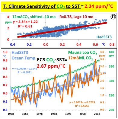
On second thought there is no ECS, because there is no observed equilibrium, it’s always transient (reference to my previous comment just posted.)
It is a shame and comical that the whole world is hung up on CO2.
Thank you very much Willis, for this indepth analysis of this vexing concept and for inspiring those very interesting comments by CO2ISNOEVIL.
a great discussion
Thanks to all participants.
oops
i was in such a hurry to submit my comment that i forgot to include the link i wanted to share
here it is ‘
https://tambonthongchai.com/2019/09/14/manabe-and-other-early-estimates-of-ecs/
it kind of goes along with the Dan Pangburn comment below where he writes about the water vapor issue
The concept of climate sensitivity ignores that CO2 is not the only ghg that has been increasing. According to NASA/RSS measurements, water vapor has been increasing about 1.5% per decade. Calculations using Hitran data show that each WV molecule is about 1.37 times more effective at absorbing the LWIR energy than a CO2 molecule. WV molecules have been increasing faster than CO2 molecules with the result that WV increase has been about 10 times more effective at warming than CO2 increase. (Forehead slap realization reduced it from 39 to 10)
A closer look at WV increase shows that the increasing trend for the last 3 decades is steeper than possible from feedback.
https://watervaporandwarming.blogspot.com
Willis, thank you again for a clear exposition of a well-focused, insightful analysis.
#comment-2879229 stuck in moderation for 4 hours now. sigh.
Willis, are you familiar with the Connolly and Connolly research?
https://andymaypetrophysicist.com/2017/08/21/review-and-summary/
the temperature profile of the atmosphere to the stratosphere can be completely explained using the gas laws, humidity and phase changes. The atmospheric temperature profile does not appear to be influenced, to any measurable extent, by infrared active gases like carbon dioxide.
Connolly and Connolly have shown, using the weather balloon data, that the atmosphere from the surface to the lower stratosphere, is in thermodynamic equilibrium. They detected no influence on the temperature profile from infrared active (IR-active) gases, including carbon dioxide. This is at odds with current climate models that assume that the atmosphere is only in local thermodynamic equilibrium as discussed by Pierrehumbert 2011 and others.
Toto, I’ve tried to follow their logic with no success. I’ve never been able to figure out how what they find with the balloons differs from what they claim it would look like if CO2 is involved.
They say, as you quote:
But I have no clue what “influence on the temperature profile” they expect. It seems they think that if CO2 affects the temperature, the atmosphere wouldn’t be in thermodynamic equilibrium … why not?
I also don’t understand what conclusion they are drawing. If it is that CO2 doesn’t absorb and emit LW, that’s clearly not true. But there’s no abstract, and no “Plain Language Summary” as we’d see in a normal journal paper, and I can’t find where they’ve laid that out.
If you have any clue where I can find the answers to those questions, I’d be interested. The paper you refer to doesn’t do it for me, at least.
Thanks,
w.
W.
I have trouble understanding them as well because I’m not qualified to. But from what I can make out, they are saying that due to the ideal gas law, the atmosphere cannot hold heat in and of itself so the extra modern heat we observe can only be due to an on-going external source. (be it from above or below) They do not say that co2 does not absorb or emit IR, only that this cannot be ”held” or ”stored” and cannot lead to a permanent increase in temps as it (co2) increases. In other words – no greenhouse effect (as it is currently understood) regardless of the composition of the atmosphere.
Probably the best starting point is a recent video of a talk and the slides from that talk:
https://youtu.be/XfRBr7PEawY
https://blog.friendsofscience.org/wp-content/uploads/2019/08/July-18-2019-Tucson-DDP-Connolly-Connolly-16×9-format.pdf
They have several levels: direct observations from weather balloons, and their interpretation regarding lapse rates, then on to new ideas about how heat energy gets transferred, and a proposed alternative to ozone heating. New ideas are of course controversial, but their weather balloon data is very interesting.
The talk goes into details about the gas laws, Boyle, Charles, Avogadro, and Ideal.
Then they talk about temperature profiles and lapse rates and why the climate models do not do these properly. And conclude that there is no need for CO2 heating to explain anything.
Their conclusions (edited):
1) The neglect of through air mechanical energy has led to the hypothesis that the atmosphere is only in local thermodynamic equilibrium i.e. conduction convection and radiation cannot transmit energy fast enough to maintain thermodynamic equilibrium with altitude . This was a mistake.
2) If the atmosphere can transmit energy quickly enough to restore thermodynamic equilibrium, our results say that it can, then […] the rate of absorption of radiation by IR active gases is equal to their rate of emission i.e. IR active gases ( so called greenhouse gases) do not trap or store energy for systems in thermodynamic equilibrium .
3) However greenhouse gases do absorb and emit radiation and can also absorb and loose energy due to collision with other gases . But […] where a thermal gradient exists, […] the net effect of greenhouse gases is to increase the flow of IR radiation from hot to cold and not the other way round.
4) […] increasing the concentrations of the so called greenhouse gases does not cause global warming.
So, I am presenting this without comment, leaving it up to readers to evaluate it themselves.
Heh heh. Who needs equilibrium, apart from climatologists?
“ain’t looking for the kind of man, baby,
Who can’t stand a little shaky ground” – Bonnie Raitt gets it…
It’s a tricky eyeball averaging process.
The raw data could give us the “correct” value for misrepresenting the data…for acquiring an ECS. But lacking that, a careful “eyeballing” can establish an upper limit…to the (probably incorrectly) calculated (estimated) ECS…and an approx upper limit to the uncertainty.
For starters, that dense patch of blue represents ~70% of the sample set and that blue blob’s average “grid cell ECS” is all well below 0.5 at around 0.25. The vast majority of the remaining 30% of the total set (the red dots) have “grid cell ECS’s” below 1.25 with far more below 0.5 than above 1.0.
So our probable misuse of the data from graph…while doing a moderately appropriate weighted averaging using ~equal area grid cells…produces a global average ECS of at most ~0.5 +/- 0.25 degrees C per CO2 doubling.
And that is likely closer to reality and less uncertain than “Charney and Onwards” 1.5 to 4.0.
“This “climate sensitivity”, often represented by the Greek letter lambda (λ), is claimed to be a constant that relates changes in downwelling radiation (called “forcing”) to changes in global surface temperature. The relationship is claimed to be:
Change in temperature is equal to climate sensitivity times the change in downwelling radiation.”
–
“The ECS measures how much the temperature changes when the top-of-atmosphere forcing changes, in about a thousand years after all the changes have equilibrated. The ECS is measured in degrees C per doubling of CO2 (°C / 2xCO2”
–
An interesting set of views encompassing the whole spectrum of Climate Sensitivity.
A lot of statements that seem to prove the different views which means that some of them must be right and some wrong
–
“There has been no advance, no increase in accuracy, no reduced uncertainty, in ECS estimates over the forty years since Carney in 1979″ consensus on the ‘likely’ range for climate sensitivity of 1.5 °C to 4.5 °C”
–
I think Willis wins with the last comment. I had thought Lewis and Curry had helped push it down but there are an awful lot of new papers trying to prove it is high. Whatever the range is ridiculous for science.
Implicit in such a wide range is that no-one agrees on a uniform description of downwelling radiation [forcing].
–
I agree with Javier in part
” While λ does not have to be a constant, if one takes a fixed point to start the doubling as Knutti does with the preindustrial value defined as the average between 1850 and 1900, that particular doubling should have a single value of λ. ”
Of course there is a constant for a specified set of circumstances.
It does have a definite value within a small range of uncertainty.
There are a few questions and a few comments further to make.
Surely with a logorithmic scale the doubling has to start at 1ppm, so how can it possibly be a constant?
Each doubling is less than the one before it, how can anyone say what the baseline for the starting was?
At low concentrations the effect of a GHG is linear, not logarithmic since the absorption lines aren’t saturated.
It is this that lies behind all those claims that various trace GHG’s like CH4 are “umpteen times stronger than CO2”.
The IR frequencies CH4 absorbs at are transparent to CO2 therefore CH4 absorbs all that IR! The fact alarmists keep prattling on about CH4 is x-times more potent a GHG than CO2 is totally bogus.
Not true if hysteresis exists within the climate system as it clearly does or say depends on the rate of change of T. The climate is not linear or invariant. Lambda can be different values depending on the direction and rate of temperature change IE dT/dt. No-one ever said that Lamba has to be directly proportional to T.
Concerning “well mixed CO2 at the surface” (Willis Eschenbach and KzTac discussion):
look here for a picture showing our surface CO2 measurements at meteoLCD (Luxembourg, Europe) where daily mixing ratio varies enormously. Mixing increases with air velocity (so it is higher, and CO2 levels lower, due to convection after noon); a long time ago I wrote a paper with the late E-G. Beck on how to estimate historic background CO2 levels from non-mixed surface measurements:
https://meteo.lcd.lu/papers/co2_background_klima2009.pdf
Thanks, Francis. The paper you linked to is quite fascinating, and answers a variety of questions that people have raised here.
Dr. Beck was kind enough to write a comment on one of my earlier posts, clarifying that his measurements were NOT of the CO2 background and could not be directly compared with it.
w.
Perhaps its because the sensitivity is so small compared to the dominant major factors that there is no way to improve what is so minute in the first place ( again in relation to the overall system) A look at saturation mixing ratios g/kg wv v temp explains, No such ratios exist for co2, because its effect on temps can not be correlated the way we can with WV
Generally the bigger, the more dominant a force, the more likely the solution lies with it
Question from a climate dummy. I keep hearing that the climate sensitivity of CO2 (not sure that’s the right phrase) is logarithmic. Skeptics say that but the supposed “consensus” is that it’s not true.
Otherwise, when I studied physics, I didn’t have much trouble with it. It all seemed so logical. To me, climate discussions are not so clear and logical. I can only conclude the subject is extremely complicated. It seems to this climate dummy that the science is not settled. If it was settled there would be few debates. I should think until it advances- we should be cautious in calling for spending trillions of dollars to fix “the problem”.
Joe
Great topic, well covered by comments – thanks
Modelling without a constant becomes a very different animal, right?
M