By Christopher Monckton of Brenchley
This will be a long posting, but it will not be found uninteresting.
Global warming on trial: Global warming goes on trial at 8.00 am this Wednesday, 21 March 2018, in Court 8 on the 19th floor of the Federal Building at 450 Golden Gate Avenue, San Francisco. Court 8 is the largest of the courtrooms in the Federal District Court of Northern California. They’re clearly expecting a crowd. The 8 am start, rather than the usual 10 am, is because the judge in the case is an early bird.
The judge: His Honor Judge William Haskell Alsup, who will preside over the coyly-titled “People of California” v. British Petroleum plc et al., is not to be underestimated. Judge Alsup, as the senior member of the Northern California Bench (he has been there for almost two decades), gets to pick the cases he likes the look of. He is no ordinary, custard-faced law graduate. Before he descended to the law (he wanted to help the civil rights movement), he earned a B.S. in engineering at Mississippi State University.

Don’t mess with me: His Honor Judge Alsup flourishing a tract by his mentor, the Supreme Court justice whom he once served as Clerk.
Six years ago, in an acrimonious hearing between Oracle and Google, the two Silicon-Valley giants were arguing about nine lines of computer code, which Oracle said Google had filched for its Android cellphone system. In preparation for the case, Oracle had tested 15 million lines of Android code, and had found that just nine lines – a subroutine known as rangeCheck – had been copied keystroke for keystroke. Oracle’s case was that these nine lines of code, though representing only 0.00006% of the Android software, were a crucial element in the system. Judge Alsup did not buy that argument.
Rumors gather about great men. In hushed tones, those who talk of Judge Alsup say he taught himself the Java programming language so that he could decide the rangeCheck case. In fact, he is not familiar with Java, but he does write computer code using qBasic, which used to be bundled free with MS-DOS. On the vast desk in his book-lined office sits a 2011-vintage Dell laptop, the only one he has that will still run qBasic. He has written programs for his ham-radio hobby, for the Mastermind board game, and for his wife’s bridge game.

The 18-year-old Bill Alsup at his ham radio console in Mississippi.
This, then, is that rarest of creatures, a tech-savvy judge. And he has taken the very rare but commendable step of ordering both parties to answer nine scientific questions about climate change in preparation for what he has called a “tutorial” on the subject next Wednesday.
Hearing of this case, and of Bill Alsup’s starring role, I wondered what line of argument might convince a scientifically literate judge that the plaintiffs, two Californian cities who want the world’s five biggest oil corporations to pay them to adapt to rising sea level, that there is no cause for alarm about manmade global warming.
Judge Alsup might well be moved to dismiss the plaintiffs’ case provided that the defendants were able to establish definitively that fears of global warming had been very greatly exaggerated.
Two propositions: If the following two propositions were demonstrated, His Honor might decide – and all but a few irredentists would be compelled to agree – that global warming was not a problem and that the scare was over.
1. It can be proven that an elementary error of physics is the sole cause of alarm about global warming – elementary because otherwise non-climatologists might not grasp it.
2. It can be proven that, owing to that elementary error, current official mid-range estimates of equilibrium sensitivity to anthropogenic activity are at least twice what they should be.
Regular readers will know that my contributions here have been infrequent in the past year. The reason is that I have had the honor to lead a team of eminent climatological researchers who have been quietly but very busily investigating how much global warming we may cause, known as the “equilibrium-sensitivity” question.
We can now prove both points itemized above, and we have gone to more than customary lengths to confirm by multiple empirical methods what we originally demonstrated by a theoretical method. The half-dozen methods all cohere in the same ballpark.
Three days before His Honor posted up his list of questions on climate science, my team had submitted a paper on our result to a leading climatological journal (by convention, I am bound not to say which until publication).
The judge’s question: When I saw His Honor’s eighth question, “What are the main sources of heat that account for the incremental rise in temperature on Earth?”, I contacted my eight co-authors, who all agreed to submit an amicus curiae or “friend-of-the-court” brief.
Our reply: Our amicus brief, lodged for us by a good friend of the ever-valuable Heartland Institute, concludes with a respectful recommendation that the court should reject the plaintiffs’ case and that it should also order the oil corporations to meet their own costs in the cause because their me-too public statements to the effect that global warming is a “problem” that requires to be addressed are based on the same elementary error as the plaintiffs’ case.
In effect, the oil corporations have invited legal actions such as this, wherefore they should pay the cost of their folly in accordance with the ancient legal principle volenti non fit injuria – if you stick your chin out and invite someone to hit it, don’t blub if someone hits it.
The judge has the right to accept or reject the brief, so we accompanied our brief with the usual short application requesting the court to accept it for filing. Since the rules of court require the brief to be lodged as an exhibit to the application, the brief stands part of the court papers in any event, has been sent to all parties, and is now publicly available on PACER, the Federal judiciary’s public-access database.
Therefore, I am at last free to reveal what we have discovered. There is indeed an elementary error of physics right at the heart of the models’ calculations of equilibrium sensitivity. After correcting that error, and on the generous assumption that official climatology has made no error other than that which we have exposed, global warming will not be 3.3 ± 1.2 K: it will be only 1.2 ± 0.15 K. We say we can prove it.
The proof: I shall now outline our proof. Let us begin with the abstract of the underlying paper. It is just 70 words long, for the error (though it has taken me a dozen years to run it to earth) really is stupendously elementary:
Abstract: In a dynamical system, even an unamplified input signal induces a response to any feedback. Hitherto, however, the large feedback response to emission temperature has been misattributed to warming from the naturally-occurring, non-condensing greenhouse gases. After correction, the theoretically-derived pre-industrial feedback fraction is demonstrated to cohere with the empirically-derived industrial-era value an order of magnitude below previous estimates, mandating reduction of projected Charney sensitivity from ![]() to
to ![]() .
.
Equations: To understand the argument that follows, we shall need three equations.
The zero-dimensional-model equation (1) says that equilibrium sensitivity or final warming ΔTeq is the ratio of reference sensitivity or initial warming ΔTref to (1 – f ), where f is the feedback fraction, i.e., the fraction of ΔTeq represented by the feedback response ΔT(ref) to ΔTref. The entire difference between reference and equilibrium sensitivity is accounted for by the feedback response ΔT(ref) (the bracketed subscript indicates a feedback response).
ΔTeq = ΔTref / (1 – f ). (1)
The zero-dimensional model is not explicitly used in general-circulation models. However, it is the simplest expression of the difference between reference sensitivity before accounting for feedback and equilibrium sensitivity after accounting for feedback. Eq. (1), a simplified form of the feedback-amplification equation that originated in electronic network analysis, is of general application when deriving the feedback responses in all dynamical systems upon which feedbacks bear. The models must necessarily reflect it.
Eq. (1) is used diagnostically not only to derive equilibrium sensitivity (i.e. final warming) from official inputs but also to derive the equilibrium sensitivity that the models would be expected to predict if the inputs (such as the feedback fraction f ) were varied. We conducted a careful calibration exercise to confirm that the official reference sensitivity and the official interval of the feedback fraction, when input to Eq. (1), indeed yield the official interval of equilibrium sensitivity.
The feedback-fraction equation (2): If the reference sensitivity ΔTref and the equilibrium sensitivity ΔTeq are specified, the feedback fraction f is found by rearranging (1) as (2):
f = 1 – ΔTref / ΔTeq. (2)
The reference-sensitivity equation (3): Reference sensitivity ΔTref is the product of a radiative forcing ΔQ0, in Watts per square meter, and the Planck reference-sensitivity parameter λ0, in Kelvin per Watt per square meter.
ΔTref = λ0 ΔQ0. (3)
The Planck parameter λ0 is currently estimated at about 0.3125, or 3.2–1 K W–1 m2 (Soden & Held 2006; Bony 2006, Appendix A; IPCC 2007, p. 631 fn.). The CO2 radiative forcing ΔQ0 is 3.5 W m–2 (Andrews 2012). Therefore, from Eq. (3), reference sensitivity ΔTref to doubled CO2 concentration is about 1.1 K.
The “natural greenhouse effect” is not 32 K: The difference of 32 K between natural temperature TN (= 287.6 K) in 1850 and emission temperature TE (= 255.4 K) without greenhouse gases or temperature feedbacks was hitherto imagined to comprise 8 K (25%) base warming ΔTB directly forced by the naturally-occurring, non-condensing greenhouse gases and a 24 K (75%) feedback response ΔT(B) to ΔTB, implying a pre-industrial feedback fraction f ≈ 24 / 32 = 0.75 (Lacis et al., 2010).
Similarly, the CMIP3/5 models’ mid-range reference sensitivity ΔTS (= 3.5 x 0.3125 = 1.1 K) and Charney sensitivity ΔT (= 3.3 K) (Charney sensitivity is equilibrium sensitivity to doubled CO2), imply a feedback fraction f = 1 – 1.1 / 3.3 = 0.67 (Eq. 2) in the industrial era.
The error: However, climatologists had made the grave error of not realizing that emission temperature TE (= 255 K) itself induces a substantial feedback. To correct that long-standing error, we illustratively assumed that the feedback fractions f in response to TE and to ΔTB were identical. Then we derived f simply by replacing the delta values ΔTref, ΔTeq in (2) with the underlying entire quantities Tref, Teq, setting Tref = TE + ΔTB, and Teq = TN (Eq. 4),
f = 1 –Tref / Teq = 1 – (TE + ΔTB) / TN
= 1 – (255.4 + 8) / 287.6 = 0.08. (4)
Contrast this true pre-industrial value f = 0.08 with the CMIP5 models’ current mid-range estimate f = 1 – 1.1 / 3.3 = 0.67 (Eq. 2), and with the f = 0.75 applied by Lacis et al. (2010) not only to the 32 K “entire natural greenhouse effect” but also to “current climate”.
Verification: We took no small trouble to verify by multiple empirical methods the result derived by the theoretical method in Eq. (4).
Test 1: IPCC’s best estimate (IPCC, 2013, fig. SPM.5) is that some 2.29 W m–2 of net anthropogenic forcing arose in the industrial era to 2011. The product of that value and the Planck parameter is the 0.72 K reference warming (Eq. 3).
However, 0.76 K warming was observed (taken as the linear trend on the HadCRUT4 monthly global mean surface temperature anomalies, 1850-2011).
Therefore, the industrial-era feedback fraction f is equal to 1 – 0.72 / 0.76. or 0.05 (Eq. 2). That is close to the pre-industrial value f = 0.08: but it is an order of magnitude (i.e., approximately tenfold) below the models’ 0.67 or Lacis’ 0.75.
There is little change that some feedbacks had not fully acted. The feedbacks listed in IPCC (2013, p. 818, table 9.5) as being relevant to the derivation of equilibrium sensitivity are described by IPCC (2013, p. 128, Fig. 1.2) as having the following durations: Water vapor and lapse-rate feedback hours; Cloud feedback days; Surface albedo feedback years.
The new headline Charney sensitivity: Thus, Charney sensitivity is not 1.1 / (1 – 0.67) = 3.3 K (Eq. 1), the CMIP5 models’ imagined mid-range estimate (Andrews 2012). Instead, whether f = 0.05 or 0.08, Charney sensitivity ΔTeq = 1.1 / (1 – f ) is 1.2 K (Eq. 1). That new headline value is far too small to worry about.
Test 2: We sourced mainstream estimates of net anthropogenic forcing over ten different periods in the industrial era, converting each to reference sensitivity using Eq. (3) and then finding the feedback fraction f for each period using Eq. (2).
The mean of the ten values of f was 0.12, somewhat higher than the value 0.05 based on IPCC’s mid-range estimate of 2.29 W m–2 net anthropogenic forcing in the industrial era. The difference was driven by three high-end outliers in our table of ten results. Be that as it may, Charney sensitivity for f = 0.12 is only 1.25 K.
Test 3: We checked how much global warming had occurred since 1950, when IPCC says our influence on climate became detectable. The CMIP5 mid-range prediction of Charney sensitivity, at 3.3 K, is about equal to the original mid-range prediction of 21st-century global warming derivable from IPCC (1990, p. xiv), where 1.8 K warming compared with the pre-industrial era [equivalent to 1.35 K warming compared with 1990] is predicted for the 40-year period 1991-2030, giving a centennial warming rate of 1.35 / (40 / 100) = 3.3 K.
This coincidence of values allowed us to compare the 1.2 K Charney sensitivity derived from f on [0.05, 0.12] in Eq. (4) with the least-squares linear-regression trend on the HadCRUT4 monthly global mean surface temperature anomalies over the 68 years 1950-2017. Sure enough, the centennial-equivalent warming was 1.2 K/century:

The centennial-equivalent warming rate from 1950-2017 was 1.2 K/century
Test 4: We verified that the centennial-equivalent warming rate in the first 17 years (one-sixth) of the 21st century was not significantly greater than the rate since 1950. We averaged the monthly global mean surface and lower-troposphere temperature anomalies from the HadCRUT4 terrestrial and UAH satellite datasets and derived the least-squares linear-regression trend (the bright blue line on the graph below).
The satellite data were included because they cover a five-mile-high slab of the atmosphere immediately above the surface, and have a coverage greater than the terrestrial measurements. The trend was found to be ![]() , equivalent to
, equivalent to ![]() /century:
/century:

Test 5: To confirm that we had understood feedback theory correctly, one of my distinguished co-authors, a hands-on electronics engineer, heard of our result and built a test rig in which we were able to specify the input signal (i.e., emission temperature TE) as a voltage, and also the direct-gain factor μ to allow for direct natural or anthropogenic forcings, and the feedback fraction β (we were using the more precise form of Eq. 1 that is usual in electronic network analysis). Then it was a simple matter directly to measure the output signal (i.e. equilibrium sensitivity ΔTeq).
The most crucial of the many experiments we ran on this rig was to set μ to unity, implying no greenhouse forcing at all. We set the feedback fraction β to a non-zero value and then verified that the output signal exceeded the input signal by the expected margin. Not at all to our surprise, it did. This experiment proved that emission temperature, on its own, induced a feedback response that climatology had hitherto overlooked.
This is where the elementary error made by climatologists for half a century has had its devastating effect. Look again at Eq. (1). The input signal is altogether absent. Although it is acceptable to use Eq. (1) to derive equilibrium sensitivities from reference sensitivities, the mistake made by the modelers was to assume, as Lacis et al. (2010) and many others had assumed, that the entire difference of 32 K between the natural temperature TN in 1850 and the emission temperature TE was accounted for by the natural greenhouse effect, comprising a direct greenhouse warming ΔTB = 8 K and a very large feedback reponse ΔT(B) = 24 K to ΔTB.
However, in truth – this is the crucial point – the emission temperature TE (= 255 K), even in the absence of any greenhouse gases, induces a large feedback response ΔTE. This feedback response to the input signal is entirely uncontroversial in electronic network analysis and in control theory generally, but we have not been able to find any acknowledgement in climatology that it exists.
Just as Lacis (2010) did, the modelers assumed that the industrial-era feedback fraction must be every bit as large as the pre-industrial feedback fraction that they had erroneously inflated by adding the large feedback response induced by emission temperature to the small feedback response induced by the presence of the naturally-occurring greenhouse gases.
It was that assumption that led the modelers to assume that there must be some very strongly positive feedbacks, chief among which was the water-vapor feedback. However, although the Clausius-Clapeyron relation indicates that the space occupied by the atmosphere can carry near-exponentially more water vapor as it warms, there is nothing to say that it must.
Suppose there were a water-vapor feedback anything like as large as that which the models have assumed (and they have assumed a very large feedback only because they are trying to explain the large but fictitious feedback fraction consequent upon their erroneous assumption that emission temperature of 255 K somehow induces no feedback response at all, while the next 8 K of warming magically induces a 24 K feedback response). In that event, atmospheric dynamics requires that there must be a tropical mid-troposphere “hot spot” [I had the honor to name it], where the warming rate should be twice or thrice that at the tropical surface. However, the “hot spot” is not observed in reality (see below), except in one suspect dataset that Dr Fred Singer scrutinized some years ago and determined to be defective.


Models predict the tropical mid-troposphere “hot spot” (top, IPCC 2007, citing Santer 2003; above left, Lee et al. 2008; above right, Karl et al., 2006).
However, the “hot spot” is not observed in reality (see below). Our result shows why not. The “hot spot” is an artefact of the modelers’ error in misallocating the substantial feedback response induced by emission temperature by adding it to the very small feedback response induced by the naturally-occurring greenhouse gases.

The model-predicted “hot spot” is not observed in reality (Karl et al. 2006).
Test 6: Even after we had built and operated our own test rig – as far as we know, this is the first time anyone has tried to test climatological feedback theory empirically rather than simply modeling it – we were not satisfied that anything other than tests performed under rigorous conditions at a government laboratory would be found widely acceptable.
Accordingly, based on the results of our in-house test rig, we drew up a more sophisticated specification for a new rig, together with four test groups comprising 23 sets of three quantities – the input signal, the direct-gain factor and the feedback fraction. Armed with the specification, I commissioned a government laboratory to carry out the experiments.
However, a problem at once arose – indeed, it was a problem with which our own engineer had wrestled. So very small were the feedback responses predicted by long-established control theory that even the presence of the operator in the same room as the test rig tended to bias the results.
Accordingly, I worked for months with a patient and amiable scientist at the government laboratory. Eventually, by somewhat altering the initial-state values specified for the 23 tests, I was able to give the scientist values that would yield results to the required precision but without loss of experimental integrity.
In due course the laboratory reported, and the results of all 23 tests – to within one-tenth of a Kelvin – were exactly as we had been able to predict theoretically. Again, the most important results were for the group of tests in which the direct-gain factor was set to unity, so that we could reassure ourselves that control theory was correct in predicting that, in the presence of a non-zero feedback fraction, even an unamplified input signal would induce a feedback response that would either amplify or attenuate it.
Another snag arose. When I had originally approached the laboratory, I had not mentioned that the research had anything to do with climate change, because all I wanted to do was to establish that we had understood the relevant control theory correctly.
When the laboratory reported, I sent it a copy of our draft paper, in which the lab results were mentioned. The laboratory panicked and said we were not allowed to use its report.
However, I had written into the contract a term to the effect that we intended to include the laboratory’s results, and a discussion of them, in an academic paper. A compromise was reached, by which we are free to include the laboratory’s results in our paper, as long as we do not mention either the name of the laboratory or the name of the scientist there who built and ran the high-specification rig for us.
The laboratory also kindly confirmed that we had represented its results fairly in our paper and had drawn justifiable conclusions from them. Furthermore, much to our pleasure, it promoted the scientist who had assisted us. He wrote us a charming letter to say that he had not allowed, and would not allow, politics to intrude into the work he had carried out for us.
With these results from a national laboratory (we cannot even mention which country it was in) we were at last content that we had established our conclusion with sufficient rigor.
The true picture: How should the 32 K difference between emission temperature and natural temperature be apportioned? Approximately 23.4 K of the 32 K is the feedback response to emission temperature; 8 K is the directly-forced warming from the presence of the natural greenhouse gases; and just 0.7 K is feedback response to that 8 K warming (panel b):

(a) Erroneous apportionment of the 32 K difference between natural temperature in 1850 and emission temperature in the absence of any greenhouse gases, given in Lacis et al. (2010).
(b) Corrected apportionment of the 32 K, allowing for the feedback response (blue) to emission temperature; the directly-forced warming from the naturally-occurring, non-condensing greenhouse gases (yellow); and the feedback response to that greenhouse warming (red).
Looking at it the other way about, if the feedback fraction were really as large as the 0.75 imagined by Lacis et al. (2010), then the Earth’s emission temperature of 255.4 K would induce a feedback response of 766.2 K, and the 8 K greenhouse warming would induce a feedback response of 24 K, so that the pre-industrial or natural temperature in 1850 would be 255.4 + 766.2 + 8 + 24 ≈ 1054 K, about three and a half times the true value of 287.6 K.
We also considered whether non-linearities in individual feedbacks might vitiate our result. However, to obtain even the 1.5 K minimum Charney sensitivity predicted by IPCC one would need to multiply at least fivefold the empirically-derived industrial-era feefdback fraction f = 0.05.
The reason why even a very large nonlinearity in the feedback sum and consequently in the feedback fraction makes little difference to equilibrium sensitivities is that the curve of equilibrium sensitivities in the presence of various feedback factors is a rectangular hyperbola (see below). Our result shows that the sensitivity calculation is not done, as now, rather close to the singularity at f = 1 (note in passing that for f > 1 Eq. (1) predicts cooling); instead, it is done at the left-hand end of the curve, where the sensitivity increases very slowly with f:

The rectangular-hyperbolic curve of Charney sensitivities in response to feedback fractions f, showing current predictions compared with the corrected result.
The outcome of the case: What will His Honor make of all this? My guess is that he will allow our amicus brief to be filed. With his engineering background, he will have no difficulty in understanding why we say that the notion of catastrophic rather than moderate global warming is rooted in the elementary physical error we have discovered.
Therefore, we hope His Honor will ask all parties to provide formal responses to our brief. On any view, it plainly raises a serious question about whether global warming matters at all – a question that strikes right to the heart not only of the case before him but of numerous other such cases now arising in several jurisdictions – and showing some evidence of careful co-ordination.
The parties will not be able to dismiss our result lightly. To refute it, they would have to show that our pre-industrial feedback fraction f = 0.08, obtained by theoretical means rooted in mainstream control theory, is incorrect; that our industrial-era value f = 0.05, obtained empirically from IPCC’s estimate of the net anthropogenic forcing to date and from the HadCRUT4 temperature record, is also incorrect; that our campaign of ten empirical calculations giving a mean feedback fraction f = 0.12, is incorrect; that the rate of observed warming over the past 68 years is either incorrect or irrelevant; that the rate of observed warming this century to date is also either incorrect or irrelevant; that the results from our test rig are inapplicable; that the results from a government laboratory are likewise inapplicable; and, above all, that it is justifiable to assume that control theory is wrong and that, per impossibile. 255.4 K of emission temperature generates no feedback at all, while the next 8 K of warming suddenly causes 24 K of feedback, as if by magic.
We do not believe in magic.
Conclusion: The anthropogenic global warming we can now expect will be small, slow, harmless, and even net-beneficial. It is only going to be about 1.2 K this century, or 1.2 K per CO2 doubling. If the parties are not able to demonstrate that we are wrong, and if His Honor accepts that we have proven the result set out publicly and in detail here for the first time, then the global warming scare was indeed based on a strikingly elementary error of physics.
The avowedly alarmist position too hastily adopted by governments and international bureaucratic entities has caused the most egregious misallocation of resources in history.
Ladies and gentlemen, we call time on a 50-year-old scam, in which a small number of corrupt and politicized scientists, paid for by scientifically-illiterate governments panicked by questionable lobby-groups funded by dubious billionaires and foreign governments intent on doing down the West, and egged on by the inept and increasingly totalitarian news media, have conspired to perpetrate a single falsehood: that the science was settled.
Well, it wasn’t.
Hello Lord Monckton and thank you for your post and your amicus brief.
I agree that some energy companies, and BP in particular, lack credibility because they have paid lip service to global warming alarmist nonsense. This happened because they had weak leadership.
I have included some comments below on:
1. The (alleged) Catastrophic Global Warming Hypothesis – dangerous human-made warming was grossly overstated and is disproved; Increasing atmospheric CO2 and moderate global warming are NOT catastrophic and are net beneficial.
2. The (alleged) Catastrophic Climate Change Hypothesis – a hypothesis so vague and ever-changing that it cannot be disproved – it is unscientific drivel.
Questions:
a. Is your estimate of ECS = ~+1.2C/(2xCO2) truly an average value, or is it an upper bound estimate (for example, assuming no natural variation)?
b. If in fact a significant part of the observed warming is later proven to be natural variation, does your ECS estimate decline below 1.2?
c. If CO2 continues to increase, and significant global cooling commences, what impact does that have on your estimate of ECS?
Regards, Allan
https://wattsupwiththat.com/2018/03/03/time-to-cool-it-the-u-n-s-moribund-high-end-global-warming-emissions-scenario/comment-page-1/#comment-2756457
[excerpts}
The hypothesis of “catastrophic manmade global warming” is already disproved by actual earth-scale data since ~1940, where atmospheric CO2 has increased while global temperature has gone down, up and sideways.
The upper-bound estimate of Transient Climate Sensitivity of ~1C/(2xCO2) by Christy and McNider (2017) is highly credible for the satellite era from ~1979 to mid-2017. This upper bound was calculated assuming (conservatively, for the sake of simplicity and clarity) that ALL the observed warming in the satellite era was due to increasing atmospheric CO2. This maximum climate sensitivity is so low that there is NO credible global warming crisis.
https://wattsupwiththat.files.wordpress.com/2017/11/2017_christy_mcnider-1.pdf
Furthermore, this maximum sensitivity of ~1C/(2xCO2) is probably about 5x to 10x too high, because we know that natural warming pre-1940 (before the rapid acceleration of fossil fuel combustion) was the same magnitude as the so-called “man-made global warming” from ~1977 to ~1997. Therefore NOT ALL the warming in the satellite era is due to increasing atmospheric CO2, and probably most or all of the observed warming was due to natural causes, just like it was pre-1940.
Within the bounds of accuracy, I suggest that the true sensitivity of Earth’s temperature to increasing atmospheric CO2 is near-zero.
The hypothesis of “catastrophic man-made climate change” is so vague it is unscientific – it is the hypo that increasing atmospheric CO2 causes everything – warmer, colder, wetter, drier, windier, etc., etc. It falsely alleges that CO2 is the “miracle molecule” that can cause everything that frightens the chronically fearful. In summary, it is utter drivel.
Regards, Allan
Lord Monckton wrote below:
“The deliberately cautious approach we took ad argumentum in preparing our paper and our brief was that all warming after 1850 was anthropogenic.”
OK – I thought so,
Therefore the ANSWERS to my questions (I think) are:
Questions:
a. Is your estimate of ECS = ~+1.2C/(2xCO2) truly an average value, or is it an upper bound estimate (for example, assuming no natural variation)? UPPER BOUND
b. If in fact a significant part of the observed warming is later proven to be natural variation, does your ECS estimate decline below 1.2? YES, SIGNIFICANTLY.
c. If CO2 continues to increase, and significant global cooling commences, what impact does that have on your estimate of ECS? IT BECOMES MUCH LOWER, OR COULD EVEN BE NEGATIVE.
I’m with Mr Macrae on a and b, but not on c. Whatever influence natural factors have on temperature, up or down, we find Charney sensitivity (i.e. equilibrium sensitivity to doubled CO2 in the air) to be positive. It is, of course, possible that, since we find Charney sensitivity to be only 1.2 K, and since solar activity is declining quite noticeably, after a sufficient period of lessened solar activity there might be net cooling. But, bearing in mind Leif Svalgaard’s estimates that the solar decline may not be as severe in the next cycle as in this one, I wouldn’t hold my breath. On balance, I expect around 1.2 K warming this century, on the assumption that there are no significant efforts to abate CO2 emissions.
Of course, if our result is correct, there will be no need to abate CO2 emissions. One less line-item of massive expenditure to unbalance the books of the nations of the West.
From the complaint:
11. The People seek an order requiring Defendants to abate the global warming-induced
sea level rise nuisance to which they have contributed by funding an abatement program to build
sea walls and other infrastructure that are urgently needed to protect human safety and public and
private property in Oakland. The People do not seek to impose liability on Defendants for their
direct emissions of greenhouse gases and do not seek to restrain Defendants from engaging in their
business operations. This case is, fundamentally, about shifting the costs of abating sea level rise
harm — one of global warming’s gravest harms — back onto the companies. After all, it is
Defendants who have profited and will continue to profit by knowingly contributing to global
warming, thereby doing all they can to help create and maintain a profound public nuisance.
——————–
So basically, at its core, this case is a money grab by cities to try and make oil companies pay for their infrastructure projects.
Why do I have the urge to yell, “bingo?”
Mr Shearer is as excited as we are. However, it will not be at all easy to get our paper through peer review. All the major climate journals have been working along different lines for decades; they have profited mightily by the error we have unearthed; and they will not go quietly into the night. But one value of discussing our idea in a leading public forum such as this is that the error is simple enough that most people with no vested interest in refusing to understand it will understand it. The idea is out now, and it can’t be put back in the bottle. The only hope the climate totalitarians now have is to find that we were wrong. But the attempts to derail our result in this thread do not even come close.
RockyRoad March 19, 2018 at 7:01 am
“Court cases typically include the process of discovery, which has been avoided by the CAGW crowd like the plague.”
If the lawyers for the Defence are competent, and with all that money behind them they should be, the Plaintiff’s documents “discovered” should be at least as illuminating as Lord Moncton et al’s killer paper.
I am not familiar with Californian or US law but, having acted as an expert in six other jurisdictions, I would be very surprised if, as already noted by Craig, Michael Mann or Hansen would be prepared to subject themselves possible cross-examination.
I will be following this case closely. I likewise am an engineer – MS/BSEE – started out in electronics building my own transmitters & receivers as a HAM operator much as this judge did. He will understand feedback and control systems based on his HAM experience and engr. background. I would imagine that given his education and experience he will probably wind up pro skeptic.
Mr Van Slooten nicely reflects the reasons why we thought it worthwhile to submit an amicus curiae brief to this particular judge. Regardless of his personal politics, he will be interested in proper scientific arguments. The judge will indeed understand the relevant principles of control theory and feedback amplification, and he will be shocked at the elementary error that has gone undetetected until now.
Judge has engineering degree = good
Judge lives in California = bad
Everyone knows
that people living in California
lose two IQ points per year.
In my day job I am styled “Her Majesty’s counsel, learned in the law” or “Q.C.” short, so let me offer this realistic comment to his Lordship.
The common law is biased against conservatism. A hundred cases dismissing a novel claim on established principles are ignored, while the outlying case allowing it will be pronounced as an “advance in the law” and become the new standard. It is this process by which the courts have turned human foetuses into lifeless protoplasm, marriage into an open source platform, and men into women or some novel gender. The post-modernists have overrun the courts, exactly like they said they would.
I sincerely hope that your truth seeking efforts bear fruit, but the chance that the learned Judge’s anticipated opinion will hold in the face of the onslaught is unlikely.
Mr Laurable should not despair. In moral questions, such as whether babies in the womb should be tortured before being dismembered, as is at present lawful, there are many possible viewpoints, though any Christiam msut oppose the torture of little babies before they are killed, by insisting that each baby earmarked for dismemberment should be given its own anesthetic first, which is not always the case at present.
But the global warming storyline is unusual in that it is allegedly based on a scientific argument – an argument that can now, for the first time, be proven to embody a significant error without which no one would expect much more than 1.2 K global warming per doubling of CO2. The courts are actually a good place to hear and examine such arguments and counter-arguments, so, in the opinion of my co-authors and me, the effort involved in submitting an amicus brief was worthwhile. If we are right, this is one judge who will come to understand that fact quite clearly, and my assessment of his character is that, whatever his previous prejudices, he will allow the scientific truth to prevail.
To confirm that we had understood feedback theory correctly, one of my distinguished co-authors, a hands-on electronics engineer, heard of our result and built a test rig in which we were able to specify the input signal (i.e., emission temperature TE) as a voltage, and also the direct-gain factor μ to allow for direct natural or anthropogenic forcings, and the feedback fraction β (we were using the more precise form of Eq. 1 that is usual in electronic network analysis). Then it was a simple matter directly to measure the output signal (i.e. equilibrium sensitivity ΔTeq).
The most crucial of the many experiments we ran on this rig was to set μ to unity, implying no greenhouse forcing at all. We set the feedback fraction β to a non-zero value and then verified that the output signal exceeded the input signal by the expected margin. Not at all to our surprise, it did. This experiment proved that emission temperature, on its own, induced a feedback response that climatology had hitherto overlooked.
I have used such an experiment to teach students how feedback works. However it doesn’t prove anything about the source of the feedback that you assert. When you assume that the pre-industrial scenario involves no GHG feedback it does not prove anything. There is no proof presented that emission temperature alone provides any feedback at all.
Phil. says “There is no proof presented that emission temperature alone provides any feedback at all.” Anticipating responses such as this, I recruited two electronic engineers and a professor of control theory to ensure that my understanding of the zero-dimensional-model equation was correct. Inherent in the correct form of that equation is the fact that, even in the absence of any direct amplification of the input signal, such as that which is driven by radiative forcings in the climate, a non-zero value of the feedback fraction will either amplify or attenuate the input signal (the emission temperature in the climate), so that the output signal is either greater or less than the input signal.
When I was in Moscow earlier this year to discuss our result with members of the Russian Academy of Sciences, I met Professor Mojib Latif, an IPCC lead author, who recommended that I should read Lacis et al. (2010), which I have cited in the head posting. Lacis’ paper actually describes the state of the climate without any greenhouse gases, and it is apparent from that description that two feedbacks – the ice-albedo feedback and the water vapor feedback, in order of importance to the pre-ghg climate – were present. However, Lacis et al. had not realized that they should explicitly account for that feedback.
Next, we built our own test rig, set the input value to 2.554 volts, gain block to unity and the feedback fraction to various non-zero values. In each instance, the output value measured on the test rig was exactly as theory had led us to predict. It was not the same as the input value. Therefore, an input signal – such as the pre-existing emission temperature in the climate – does indeed induce a non-zero feedback response in the presence of a non-zero feedback fraction.
We know that climatology would be unfamiliar with the relevant feedback theory. So we made assurance doubly sure by inviting a government laboratory to build a test rig to our specification. The laboratory revised our specification, built the rig and carried out the 23 tests we had requested, four of which were directed at establishing whether there was a feedback response to the input signal. The laboratory’s report, which is annexed to our paper now under peer review at a leading climate journal, makes it clear that there is indeed a feedback response even to an unamplified input signal.
Once we had established this fact, it was a simple matter to recast the zero-dimensional-model equation as in Eq. (4) in the head posting and then to derive the pre-industrial feedback fraction directly, but this time allowing for the feedback response to emission temperature.
Next, we used that feedback fraction in climatology’s form of the zero-dimensional-model equation, discovering that Charney sensitivity would then be 1.2 K and not the CMIP models’ 3.3 K mid-range estimate.
Then we derived the industrial-era feedback fraction from IPCC’s mid-range estimate of the net anthropogenic radiative forcing from 1850-2011 compared with the total observed warming over the same period. The result was a feedback fraction very close to the pre-industrial value – so close, in fact, that the Charney sensitivity derivable from it was near-identical to that derived from the pre-industrial value.
Then we checked that the centennial-equivalent warming rate since 1950, which is approximately the same as Charney sensitivity, for the reasons explained in the head posting. The result was again 1.2 K/century.
We do not think we have left very much wriggle-room except at the margins of our argument. A serious error has been made, discovered, exposed, proven and quantified, and, upon correction of that error, there is no longer a global-warming problem. The error caused the apparent problem.
Game, set, match.
i am really glad phil asked that question the way he did and for the response lord monckton .i was concerned that i understood what you propose far too easily. if i can understand the basics anyone can, especially after reading your response to phil.
Monckton of Brenchley March 19, 2018 at 12:19 pm
Phil. says “There is no proof presented that emission temperature alone provides any feedback at all.” Anticipating responses such as this, I recruited two electronic engineers and a professor of control theory to ensure that my understanding of the zero-dimensional-model equation was correct. Inherent in the correct form of that equation is the fact that, even in the absence of any direct amplification of the input signal, such as that which is driven by radiative forcings in the climate, a non-zero value of the feedback fraction will either amplify or attenuate the input signal (the emission temperature in the climate), so that the output signal is either greater or less than the input signal.
When I was in Moscow earlier this year to discuss our result with members of the Russian Academy of Sciences, I met Professor Mojib Latif, an IPCC lead author, who recommended that I should read Lacis et al. (2010), which I have cited in the head posting. Lacis’ paper actually describes the state of the climate without any greenhouse gases, and it is apparent from that description that two feedbacks – the ice-albedo feedback and the water vapor feedback, in order of importance to the pre-ghg climate – were present. However, Lacis et al. had not realized that they should explicitly account for that feedback.
Next, we built our own test rig, set the input value to 2.554 volts, gain block to unity and the feedback fraction to various non-zero values. In each instance, the output value measured on the test rig was exactly as theory had led us to predict. It was not the same as the input value. Therefore, an input signal – such as the pre-existing emission temperature in the climate – does indeed induce a non-zero feedback response in the presence of a non-zero feedback fraction.
Well water vapor feedback is a GHG feedback.
Your ‘test rig’ sounds like the one I use in my class, basically use an Op amp with an input of 2.554V and use a resistance feedback ratio of 10 kohm/100kohm gives you a gain of 1.1 so an output voltage of 2.809V. Fine but it doesn’t tell you anything about the source of the feedback in the system being modeled. If you wanted to model albedo feedback you’d need to add a positive feedback loop as well.
Phil. says water vapor feedback is a greenhouse-gas feedback. However, as the head posting (worth reading before commenting) makes explicit, we are considering the forcings from the non-condensing greenhouse gases. Water vapor is a condensing greenhouse gas; changes in its atmospheric burden are consequently expressed in climatology as feedbacks.
And of course our method tells us nothing of the sources of feedback in the system, except that the emission temperature itself induces a feedback response. We have adopted a top-down approach, taking all feedbacks as simply additive and thus working only with the feedback sum, which becomes the feedback fraction when multiplied by the Planck parameter.
It seems to me that if you look at this a little differently you can easily see that MoB is correct. Assume the sun only provided 200 K or 100 K or any level of emissions input. Let the system stabilize. Now, crank up the sun to 255 K. Would we expect feedback from the additional warming?
The answer is obviously yes. It looks like Phil. is digging.
Good Lord, Monckton of Brenchley! You’ve launched a legal and physics armed torpedo directly at the boiler room of the CAGW flagship People of California!
My sincere hope is the court accepts your amicus brief submission and further asks the litigants for critical response to the physics based arguments you present there. It will be very interesting to see what ‘evasive maneuvers’ are attempted by the People of California, as your physics armed torpedo closes in. We may all be witness to a true ‘tipping point’ in CAGW science….
J Mac is right. Time to order popcorn, sit back and watch the fun. Our multiple empirical methods, all confirming the original theoretical result, will make it uncommonly difficult for the plaintiffs to overthrow our result. The truth is that an elementary error of physics has been made; it is a serious and material error of physics; and, after correcting the error, there was and is no basis for alarm about global warming. We do not think the plaintiffs will be able to overthrow those conclusions at all – and certainly not convincingly enough to justify any order of the court against BP and the other large oil corporations.
please don’t argue that a temperature creates its own feedback. The proper way of saying it is that there had to be an initial feedback to get the temp up to the temp of 1850. That could not have been caused by the little amount of CO2 in the atmosphere immediately preceeding 1850. However the proper way of explaining it to the judge is this. In the beginning there was no water vapour in the atmosphere because the only physical way that it could get there in appreciable quantities is by evaporation. Evaporation can only happen if the air temperature is significantly higher than the ocean temperature. So to start the process of evaporation there were massive amounts of CO2 in the atmosphere 4.6 billion years ago . If the atmosphere did not have CO2 in it there would have been no way to increase the temperature. So CO2 enabled a temperature increase. Gradually as plants evolved on earth they absorbed the CO2 from the atmosphere and the CO2 levels went down to dangerous levels over time. so at the time of 1850 most of the K above the emission temperature was because of the H2O and not the CO2. The CO2 initially caused H2O forcing 4.6 billion years ago but since then it is the H2O feedbacks that keep the temperature moderate. Since 1950 mankind has caused slight increases of CO2 and we are getting a slight feedback from increased CO2 but it is so tiny that it is laughable. We need all the CO2 that we can get. The very slight temperature changes from the CO2 proves that the alarmist position is untenable. For their alarmist theory to work they need a massive feedback ( ie increase) of H2O vapour but H2O vapour has been constant in the atmosphere since 4.6 billion years ago. Tell the judge that James Hansen of the Goddard Space Institute shut down the water vapour measuring section after 20 years when he couldn’t show any increase of water vapour in the atmosphere. Without an increase of water vapour the tiny amount of CO2 cant force very much.
Mr Tomalty says I should not argue that a temperature creates its own feedback. But that is not what I am arguing. I am arguing that if feedbacks are present (denominated in Watts per square meter per Kelvin), then if a temperature is also present there will be a feedback response.
San Francisco has tide gauge data dating back to 1854. It shows a constant SLR trend of 1.96 mm / yr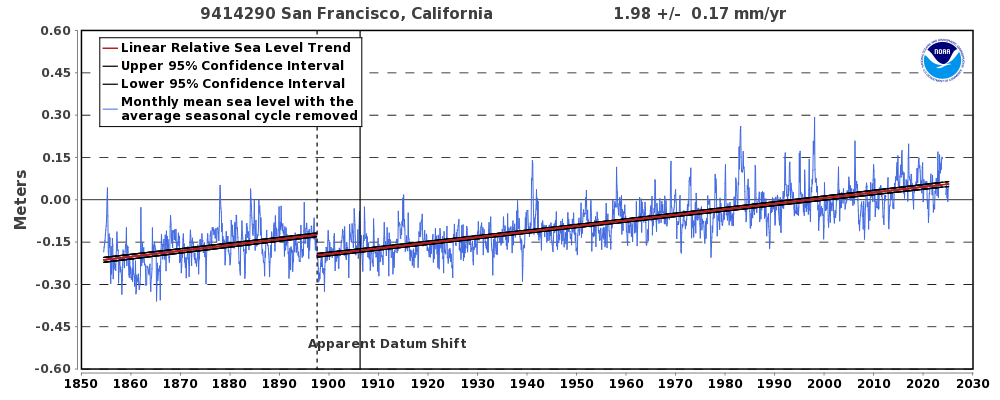
That will be a another bit of a problem for the goofy plaintiff cities.
Robin of White Rock – The approach of hoisting the AGW enthusiasts on their own petard is classic. Well done, best of luck!
A further thought to offer on this post, reconciling observational ECS (energy budget models and the like, see long comment upthread) to this new simpler more rigorous approach. The inherent problem in all the observational ECS approaches is they do not and cannot account for attribution—what part of the observed delta t is natural rather than AGW induced. See guest post Why Models Run Hot for a simple explanation not explicitly in an ECS setting. We know there is significant natural variation (MWP, LIA, comparing 1920-1945 to 1946-1975 to 1975-2000), but not why or how much. Removing natural variation was the essence of Manns infamous hockey stick. So ECS must be lower than ‘observed’ but that is all that could be said. This new approach ismindependent of natural variation and solves only for pure AGW induced ECS.
AND that suggests that if feedback free CO2 doubling ECS is 1.1 as given in this post, and with feedbacks it is 1.2, and observationally (energy budget method) with best current aerosol estimate it is 1.5, then (1.2-1.1=) 0.1 divided by (1.5-1.1=) 0.4 means 25% of the last century’s observed warming is AGW and 75% is natural variation. WOW!
IPCC AR5 WG1 has wrming since 1950 explicitly mostly AGW “with high confidence”. So this corrollary conclusion is a separate fatal body blow to the warmunist belief system.
Mr Istvan is, as always, most interesting. I shall think further about his suggestion that our result provides a method of deriving the fraction of post-1950 warming that is anthropogenic. The deliberately cautious approach we took ad argumentum in preparing our paper and our brief was that all warming after 1850 was anthropogenic.
Why guess,
and likely be wrong ?
Just use a range.
BEST CASE:
All post-1950 warming is natural, to
WORST CASE
All post-1950 warming is from man made CO2.
Wouldn’t the “correct answer”,
for CO2 effects alone,
likely be somewhere in that range ?
FEEDBACKS:
Unknown — not even whether negative or positive
so there’s no logical reason for any single guess,
or any range of guesses.
And please use weather satellite data when available
since 1979 —
— surface data are not even close to being global,
with all the wild guess infilling, and multiple “adjustments”.
“IPCC AR5 WG1 has wrming since 1950 explicitly mostly AGW “with high confidence”.”
Common sense ruled that out all along, imo,(1910 to 1940) but why were the authors of that statement so off base? MBs work provides a clear reason for how the models got it wrong. Great work.
SB, the explicit IPCC brief from the beginning was AGW. AR4 WG1 SPM fig 4 used the contrast between warming 1920-1945, explainable ‘naturally’ (not enough delta CO2 forcing in the period) and the warming 1975-2000 ‘explainable’ in models only with AGW forcings and not natural forcings to argue the later warming was all AGW. The fatal logical flaw in that figure is the two periodsare essentially indistinguishable. Natural variation did not magically stop in 1975. The attribution problem has been an IPCC Achilles heel. As suggested by my comment, on the surface from this post the new paper puts an arrow through it.
I’m very curious as to the crickets I’m hearing from the normal BEST commentator we get on this blog whenever the Lord posts.
Sun Spot
did you mean abnormal
BEST commentator ?
The claim that the First IPCC report predicted 1.35C warming from 1990 – 2030 was made in the previous posting from Monckton of Brenchley, and I disagreed with it then. Page xxii and graph make it clear that they their model assumes temperatures in 1990 were 1C above pre-industrial levels. This means that the stated rise of 1.8C from pre-industrial levels made on page xxiv is predicting 0.8C warming from 1990 to 2030, a rate of warming of 2C / century, not the 3.3C / century claimed here.
In response to Bellman, we did not need to accept IPCC’s assumption of 1 K warming from the pre-industrial era to 1990, since we know from the HadCRUT4 dataset, which IPCC said it was using, that only 0.45 K of warming had occurred since 1850.
Besides, the prediction on p. xiv of IPCC (1990) is not the only prediction made by IPCC. It also predicted 1 K warming from 1991-2025, a centennial-equivalent rate of 3 K.
You do need to know what the IPCC considered the rise since pre-industrial times to be if you want to know what they meant by 1.8C warming. They said (page 199) that there had been 0.45 ± 0.15C since the late 19th century, not “pre-industrial”. But this is irrelevant to how they expressed the projections.
As you say on page xxii the projection is 1C to 2025, “about 2C above that of the pre-industrial period.”. Similarly they say 3C warming to the end of the century, (about 4C from pre-industrial). And the companion graph clearly shows about 1C warming by 1990. Why would they be using a completely different base line two pages later?
I don’t know why there is a difference between the projected warming on the two pages, but you were the one who insisted on using the slower rate from page xxiv. But neither shows this claimed 3.3C / century.
The climate sensitivity is undoubtedly too large, but it’s not reasonable to use an absolute temperature for a differential feedback.
Scottish “Sceptic” should know me better than to imagine that I would use an entire temperature as the input and then not use an entire temperature as the output. The head posting makes it quite clear how we did the calculation. The method was recommended by a professor of control theory, and we tested it at a government laboratory as well. The simple point is that there is a feedback response of about 23.4 K to the 255.4 K emission temperature; that there is a feedback response of about 0.7 K to the 8 K directly-forced warming caused by the presence of the naturally-occurring, non-condensing greenhouse gases; and that, therefore, the pre-industrial feedback fraction is of order 0.08, and not the currently-estimated values an order of magnitude above that value.
I can’t say this is your strongest paper. As such I would recommend drawing the judges attention to the following:
1. The ~1C predicted effect of CO2 alone. I would also highlight the way this critical figure is all but missing from the IPCC report (It seems the IPCC denies the science in the biblical sense as it just doesn’t want to admit this figure exists – I have only found it as a footnote in one report – something that is truly bizarre as that ~1C is supposedly the “settled science”).
2. That the IPCC estimates are based on feedbacks – which are unproven and in no sense “settled science”.
3. That as a result of 1& 2 that the bulk of estimates for warming is not based on “settled science” but wishful/doomsday thinking of academics
4. That the satellites show a pause.
5. That the satellites are corroborated by radio sonde data.
6. That surface data has been heavily corrupted.
7. That there have been ~52 excuses for the pause and almost without except an potential cause for the, pause is also a potential explanation for the post cooling scare to pause warming. Therefore the common claim that “nothing but CO2 could have done it” is total non-science.
“it’s not reasonable to use an absolute temperature for a differential feedback”
Absolutely (no pun)!. I’m glad to see there is one at least sceptic in Scotland. Lord M’s error is in a para appropriately headed “The error”. It says
“Then we derived f simply by replacing the delta values ΔT_ref, ΔT_eq in (2) with the underlying entire quantities T_ref, T_eq, setting T_ref = T_E + ΔT_B, and T_eq = T_N (Eq. 4)”
I’m dubious about the claim that
f = 1 –T_ref / T_eq
if for no other reason that the claim that 8K of the 32K is due to non-condensing GHGs is very hard to establish. The effects aren’t just linearly additive. You can’t just take out one component of the gases and say the effect would reduce proportionately. It’s like trying to estimate what fraction of the effect of a traffic jam is due to the red cars.
But anyway, the effect could be rewritten
f = (T_eq –T_ref) / T_eq
Now you see what happens when you replace temperatures by absolutes (for which no justification is given). The numerator remains a difference, unchanged. But the denominator has 273K added to it. So of course f goes way down. And there is no role for absolute zero here. It’s just changing to a different scale. You could add anything, and make f anything you want.
f = 1 –T_ref / T_eq
But anyway, the effect could be rewritten
f = (T_eq –T_ref) / T_eq
Now you see what happens when you replace temperatures by absolutes
============================
Your rearrangement of the equation makes absolutely no difference to the result.
An absolute minus and absolute is still an absolute.
if one looks at Monckton’s posted work:
f = 1 –Tref / Teq = 1 – (TE + ΔTB) / TN
= 1 – (255.4 + 8) / 287.6 = 0.08. (4)
using Nic’s rearranged equation we get:
f = (T_eq –T_ref) / T_eq
= (287.6 – (255.4 + 8))/287.6
= (287.6 – 263.4)/287.6
= 24.2/287.6
= 0.08 !!!!
Perhaps we should rename this the “Stokes Effect” – absolutely no affect.
“Your rearrangement of the equation makes absolutely no difference to the result.”
Exactly. But it shows the difference that the unjustified switch to “entire” values makes. The first calc was a ratio between two differences, which could be C or K
f=24.2/32.2 = .75
The second just adds 255.4 to the numerator but not the denominator
f=24.2/(32.2+255.4) = .08
It is the ratio of a difference to an absolute.
“to the numerator but not the denominator”
other way round.
It isn’t clear how Monckton went from 2 to 4 (below), which I understand is what Scottish Sceptic is saying. Hopefully this is addressed in the full paper. However this isn’t what I read Nic’s algebra to be saying.
Question: how were the delta’s removed between (2) and (4)?
f = 1 – ΔTref / ΔTeq. (2)
f = 1 –Tref / Teq = 1 – (TE + ΔTB) / TN
= 1 – (255.4 + 8) / 287.6 = 0.08. (4)
“how were the delta’s removed between (2) and (4)?”
By hand-waving. No justification is offered. And none is possible.
In answer to Mr Stokes and Mr Berple, I begin with the observation that a temperature feedback is a response to temperature and not, as Mr Stokes imagines, a response to forcing. Accordingly, if the conditions precedent to the occurrence of a feedback response obtain in the climate system, then a temperature subsisting in that system will induce a temperature-feedback response.
Consider, first, a climate system which possesses something like today’s albedo but no non-condensing greenhouse gases. From the SB equation, the insolation and the albedo, we know that the temperature in the absence of any greenhouse gases or feedbacks will be 255 K or thereby. However, as Lacis et al. (2010) point out, even in the absence of the non-condensing greenhouse gases there would be open water at the equator, implying an ice-albedo feedback, and there would be some water vapor in the atmosphere, implying a water vapor feedback and a cloud feedback.
Let us, then, derive the feedback response to emission temperature, using the method that is standard in control theory. The input signal is 255.4 K; the direct-gain factor in the gain block is unity (for there are no greenhouse gases to amplify surface temperature yet); and the feedback faction is – illustratively – 0.084. Then the output signal is 255.4 / (1 – 0.084), which is 278.8 K. The difference between the input and output signals is the feedback response, i.e. 23.4 K.
Now add some greenhouse gases. Lacis et al. (2010) imagine that some 24 K, or three-quarters of the 32 K difference between emission temperature and the natural temperature that obtained in 1850 is the feedback response to 8 K of directly-forced warming attributable to the presence of the naturally-occurring, non-condensing greenhouse gases.
In fact, that 8 K of direct warming is the direct gain in the feedback loop. From this we may determine the direct-gain factor, labeled mu in Bode (1945). It is simply 1 + 8 / 255.4, or 1.0313. Now, assuming illustratively that the feedback fraction (beta in Bode) is constant throughout the pre-industrial era, one calculates thus: Equilibrium temperature after feedback (i.e., the output signal) is equal to the emission temperature before feedback (the input signal 255.4 K) multiplied by the ratio of mu to (1 – mu * beta). In this example, then, the equilibrium pre-industrial temperature after allowing feedback is 255.4 x 1.0313 / (1 – 1.0313 * 0.082), or 287.7 K, which is about right. Note that 0.082 is very slightly smaller than 0.084 because we have set mu to a value above unity to allow for the 8 K direct warming in response to the presence of the naturally-occurring, non-condensing greenhouse gases.
Or one could use the assumption implicit in official climatology that mu is equal to unity (this isn’t too bad an assumption, because mu is quite close to unity). Then equilibrium pre-industrial temperaturein 1850 is (255.4+8) / (1 – 0.084), or 287.6 K, which is about right.
It comes as a great surprise to the climatological community that a feedback arises even in the absence of a direct gain factor mu. You will see later in this thread that it was at this point that I lost Roy Spencer. Many other climatologists have expressed similar surprise. That is why I recruited not only two engineers with practical experience of feedback but also an adjunct professor of applied control theory (he gets tenure later this year) to assist in ensuring that the control theory was correctly represented in our paper.
It matters not that the models do not explicitly incorporate the zero-dimensional model. We calibrated the ZDM by taking the official CMIP5 inputs in Vial (2013), used by IPCC (2013), and plugging them in. We obtained the interval 3.3 [2.0, 4.5] K that is the CMIP5 models’ climate-sensitivity interval.
Likewise, it matters not that the difference between emission and surface temperature woulkd be 72 K rather than 32 K in the absence of convective processes. The ZDM takes the system as it finds it.
The key point in all this is a very simple one. If conditions precedent to a feedback response are present in a dynamical system, then any input to that system, whether or not it is amplified, will induce a feedback response. In this sense, there is no distinction (except at the margins) between the emission temperature that is the input signal and the directly-forced 8 K of additional temperature caused by the presence of the greenhouse gases. If one assumes that the 8 K induces a feedback response, it is inconsistent to assume that the 255.4 K induces no feedback response at all.
“how were the delta’s removed between (2) and (4)?”
By hand-waving. No justification is offered. And none is possible.
==============
Nic (and Monckton), I’ve gone through the arguments and after a long walk with the dog to think things through I believe Monckton is correct, with a small quibble. Here is the reason:
The 255K temperature is both an absolute and a delta!! This is obscured somewhat by the use of the words temperature and forcing to represent similar ideas by different people on this site, depending on background.
What the 255K temperature represents is effective temperature of the earth due to the sun. In the absence of the sun the earth’s effective temperature would be 0K. Thus the delta would also be 255K. So when people talk about temperature and forcing, they are really talking about the delta attributable to the sun.
So there is no problem in going from (2) to (4). For example: 255K – 0K = 255K
My small quibble is that the earth would not be 0K without the sun. It would be 3K due to CBR. Thus, the equation should probably have been written something like:
f = 1 – ΔTref / ΔTeq = 1 – (TE – CBR + ΔTB) / (TN – CBR)
= 1 – (255.4 – 3 + 8) / (287.6 – 3)
= 1 – 260.4/284.6 = 0.085. (4)
However, I don’t believe this alters the result significantly. I could well be that 3K was not considered previously in calculating 255K, and can be ignored. However, in the interest of completeness, Monckton may wish to review this small point.
ferd,
“In the absence of the sun the earth’s effective temperature would be 0K.”
If you want to include the effect of absenting the sun in the input, you have to include it in the response. But the response remains 24.2K. That obviously does not include the response to absence of sun.
The other thing about all this is that gain and feedback are responses to small changes. They represent derivatives of the state variables. Taking the notion of a single feedback coefficient to a 32K variation is a stretch. Taking it to a 255 K variation is ridiculous.
Lord M,
“The input signal is 255.4 K”
Again, just wrong. A signal is a change. If you want to think about a change from 0 to 255K, you need to divide it into the response to that change. And a feedback determines a proportional response. If the Earth had half as much GHG, it is reasonable to expect a 16K differential, of which 4K is due to GHG. Your arithmetic is going to give a feedback factor then of 12/(255+4)= 0.046, not 0.08. In fact, , if the GHG component was a small fraction g of what we do have , the feedback factor would be about 0.08*g. But the gain andfeedback factor should not depend on the size of signal, especially when small. It is a property of the control system.
Mr Stokes is, with respect, simply wrong about whether the emission temperature is a “signal”. It is. It is the “input signal” in the dynamical system that is the climate. And, even in the absence of greenhouse gases, it induces a feedback, whose magnitude we derived theoretically and then verified using not one but two test rigs. Bode (1945, ch. 3) applies the term “signal” to the input voltage and the output voltage in a feedback-amplifier loop. A temperature feedback is a feedback that arises owing to the presence of a temperature. The magnitude of the temperature feedback response is dependent upon the magnitude of the temperature.
Mr Stokes is also confused about the relative magnitudes of the constituents in the 32 K difference between natural temperature in 1850 and emission temperature in the absence of greenhouse gases or feedbacks. We know that the difference is 32 K. he question, therefore, is how to apportion it. Lacis et al. (2010) say 75% of it is feedback response, wherefore 25%, or 8 K, is the directly forced greenhouse warming. Suppose one thought that 8 K should really be 11 K. Then the feedback fraction would work out at 1 – (255.4 + 11) / 287.6, or 0.074. Suppose there were no greenhouse forcings at all. Then the feedback fraction would be 1 – 255.4 / 287.6, or 0.11, which is the impossible maximum pre-industrial feedback fraction. The truth is that we do not know exactly how large the directly-forced warming from the naturally-occurring, non-condensing greenhouse gases is, so we have simply taken Lacis’ estimate as an illustrative example. Other estimates might be made, but they do not much alter the value of the feedback fraction.
” It is the “input signal” in the dynamical system that is the climate. And, even in the absence of greenhouse gases, it induces a feedback”
So what is the response to the 255K “input signal” alone? That is then modified by feedback? I asked that before, and got no answer.
As I noted elsewhere, the arithmetic promoted here would say that the feedback factor is proportional to the amount of GHG added to the air, and would be zero if there were none (since the 255K provides zero response). But the feedback factor is a property of the system and should not be proportional to the signal.
here is the problem between Christopher and Nick
The real graph should be 31.4K due to clouds and H2O and 0.8K due to CO2,methane…etc
how do I get that For the longest time CO2 levels before 1850 were at dangerous levels for plant growth( they would die at 150ppm) Therefore the initial feedback 4.6 billion years ago was what caused the water vapour to be the level it is in the atmosphere. So Co2 is a minor player. However as long as Monckton stops saying that a temperature causes a temperature…….. he is completely correct. See below for complete explanation
Please don’t argue that a temperature creates its own feedback. A temperature isnt a real entity. It is only a measurement. The proper way of saying it is that there had to be an initial feedback to get the temp up to the temp of 1850. That could not have been caused by the little amount of CO2 in the atmosphere immediately preceeding 1850. However the proper way of explaining it to the judge is this. In the beginning there was no water vapour in the atmosphere because the only physical way that it could get there in appreciable quantities is by evaporation. Evaporation can only happen if the air temperature is significantly higher than the ocean temperature. So to start the process of evaporation there were massive amounts of CO2 in the atmosphere 4.6 billion years ago . If the atmosphere did not have CO2 in it there would have been no way to increase the temperature. So CO2 enabled a temperature increase. Gradually as plants evolved on earth they absorbed the CO2 from the atmosphere and the CO2 levels went down to dangerous levels over time. so at the time of 1850 most of the K above the emission temperature was because of the H2O and not the CO2. The CO2 initially caused H2O forcing 4.6 billion years ago but since then it is the H2O feedbacks that keep the temperature moderate. Since 1950 mankind has caused slight increases of CO2 and we are getting a slight feedback from increased CO2 but it is so tiny that it is laughable. We need all the CO2 that we can get. The very slight temperature changes from the CO2 proves that the alarmist position is untenable. For their alarmist theory to work they need a massive feedback ( ie increase) of H2O vapour but H2O vapour has been constant in the atmosphere since 4.6 billion years ago. Tell the judge that James Hansen of the Goddard Space Institute shut down the water vapour measuring section after 20 years when he couldn’t show any increase of water vapour in the atmosphere. Without an increase of water vapour the tiny amount of CO2 cant force very much.
“The real graph should be 31.4K due to clouds and H2O and 0.8K due to CO2,methane…etc”
That gives feedback f=39. Lord M says 0.08. I think Lacis is better, with something around 3.
In reply to Mr Tomalty, a temperature feedback is indeed a feedback to temperature. Temperature feedbacks are denominated in Watts per square meter per Kelvin of the temperature (or temperature change) that induced them. If Mr Tomalty wishes to take issue with official climatology in this respect, he should address his concerns not to me but to the IPCC. My policy has been to adopt ad argumentum all aspects of official climatology except those that now require correction as a result of the error of physics we have found.
“If Mr Tomalty wishes to take issue with official climatology “
No, “official climatology” doesn’t talk much about feedback at all. But when it does, it is feedback to a forcing.
Mr Stokes, who believes that official climatology hardly talks about feedback at all, may care to read the Fifth Assessment Report of the Intergovernmental Panel on Climate Change, where the word “feedback” occurs >1100 times. After all, official climatology imagines that feedbacks increase reference sensitivity by a factor 2 to 10, mid-range estimate 3.
He is, of course, correct that official climatology defines a feedback as a response not to an entire temperature but to a temperature change. But that, of course, is precisely the error that official climatology is making. It can attempt to define a temperature feedback that way till it is blue in the face, but that does not in any way alter the fact that, as the zero-dimensional-model equation makes quite clear, and as our two feedback-amplifier circuits confirm, the Earth’s emission temperature will itself induce a feedback response, since temperature feedback processes will necessarily respond in the presence of a temperature.
Thanks, Christopher, for an impressive effort. I hope it has the desired result.
My observations:
A. I appreciate the general thrust and logic, but in places there appears to be an implicit assumption that the feedback fraction (or ratio) is constant. That seems very unlikely to me. That part of the argument does still appear to be valid – it’s just that it can’t be given exact numbers.
B. Your “Conclusion: The anthropogenic global warming we can now expect will be small, slow, harmless, and even net-beneficial.” is misleading by omission. There is no reason to suppose that the higher rate of warming predicted by the IPCC would not also be net-beneficial. [Note: I deliberately use the word “predicted”, as per the duck look walk quack maxim.].
Typos? Or my misunderstanding?
1. “Abstract: In a dynamical system, even an unamplified input signal induces a response to any feedback.”. Should this be “… induces a feedback response”?
2. Just after equation (3), this doesn’t look right to me: “The Planck parameter λ0 is currently estimated at about 0.3125, or 3.2–1 K W–1 m2”. Should this be “-3.2 K W–1 m2”?
3. In the paragraph before “The new headline Charney sensitivity”, should “There is little change that some feedbacks had not fully acted.” be “There is little chance that some feedbacks had not fully acted.”?
Apologies if these comments have already been made. I haven’t yet read the comments.
I am most grateful to Mr Jonas for the trouble he has taken.
As to the assumed constancy of the feedback fraction, of course that is an jillustrative assumption. Lacis et al. (2010) explicitly assume it in holding that the feedback fraction induced by “the entire greenhouse effect” is 0.75 and that the feedback fraction “for today’s climate” is likewise 0.75,.
We derived the pre-industrial feedback fraction theoretically and found it to be of order 0.08. We separately derived the industrial-era feedback fraction empirically and found it to be of order 0.05. What these results, obtained by distinct methods, appear to indicate is that the feedback fraction is so small that any nonlinearities are de minimis.
As to the conclusion, I agree with you that even 3 K warming per doubling of CO2 would probably not be harmful, a point that the formidable Dick Lindzen has often made.
As to the wording of the abstract, it is as it is because there cannot be a feedback response except in the presence of some feedback.
As to the Planck parameter, 0.3125 is, as shown in the head posting, the reciprocal of 3.2, i.e. 3.2 to the power of minus 1.
As to “change” where “chance” is intended, I apologize for the misprint.
Naturally, Lord Monckton, this is a wonderful reading; however I wonder . . “If the following two propositions were demonstrated, His Honor might decide – and all but a few irredentists would be compelled to agree – that global warming was not a problem and that the scare was over.”
” . .that global warming . .'”
Why not always be more specific – saying, ” . . that man-made global warming, AGW, is not a problem.
I propose that we should always distinguish between what we believe to be naturally occurring GW and/or CC, and that, which they believe to be some serious issue, AGW and ACC, or CACC.
My response when someone asks me, if I believe in GW, or CC, always begins with – ‘can you be more specific, pls?”
In answer to Garyh845, I agree that one could be more specific about the conclusion that manmade global warming, rather than just global warming, is not a problem.
Thanks very much. Actually, Judith Curry wrote about this topic once a couple of years back.
PS – ‘one should,’ not ‘one could.’ That was the whole point. If folks are pressed into understanding the difference between naturally occurring climate change – constantly dramatic as it is – and the view that some additional bit of GW (potentially caused by AGHG emissions) is predicted – by some – to have an effect on that, then I propose that they might be more willing to engage themselves in an intelligent internal debate on the issue.
(;~> gary
I made it all the way through the comments and did not see any coherent objection. That means I am going to accept the argument as it stands. As always I am thrilled by Monckton’s erudition and rhetorical skills. This is what draws me back to WUWT. Well done and good luck!! A very commendable effort. Semelweiss, Wegener and Margulis will be watching.
I’d like to hear RG Brown weigh in on this. His endorsement would be gratifying, and his style would be a pleasure to read, like M’lud’s.
What is the actual experiment that illustrates that Co2 causes warming . If it is the co2 in the test tube experiment , how many ppm of co2 are used?
I’ll try to answer because you have
a wonderful first name, Richard:
After 20 years of reading about climate change
the lack of real science is stunning.
Simple lab experiments —
—using infrared absorption
spectroscopy (IRS)
— determined the infrared
absorption spectrum of CO2.
The lab experiments only prove
CO2 is a greenhouse gas.
A greenhouse gas should cause warming,
mainly at night.
No one knows how much warming,
and it is impossible to know.
We also don’t have accurate
surface temperature measurements
to make am accurate guess.
But the satellite measurements
are near global and better
— they start in 1979 —
but most of the warming attributed to CO2
by the IPCC is after 1975 ,
and 1975 is close to 1979.
We can guess a
WORST CASE warming,
from CO2 alone,
net of feedbacks,
which are a mystery
so there’s no need
to wild guess feedbacks
If you start by assuming
ALL all warming
in the satellite era,
since 1979,
was caused by CO2,
which is a worst case warming
from CO2 assumption,
then you could speculate
that a doubling of CO2,
in 125 years
(at +3 ppm per year)
to 200 years
(at +2 ppm per year),
would increase
the average temperature
by about + 1 degree C.
long after you are dead !
Mainly warming at night
in colder, dryer latitudes
= ho, hum, harmless !
I wrote an article titled:
“Climate Science is Missing the Science”
in simple, plain English,
because I believe I know enough
about the subject to keep it simple,
at the following URL
http://elonionbloggle.blogspot.com/2018/03/climate-science-is-missing-science.html
There is another issue that has never been acceptably addressed: What is the optimum temperature of the earth to support life?
Life has generally thrived at higher average temperature and suffered at lower average temperature. but what is the optimum? That has never been determined and would vary considerably depending on what criteria are used. Which lifeform or forms are the benchmark? Which area of the earth is also of concern. If warming opens up vast areas of unused land, isn’t that to the benefit of mankind. Canada would welcome a few degrees increase in average temperature.
I am dumbfounded by my fellow Canadian’s refusal to acknowledge the possibility of a net benefit to Canada from warming. The thoroughness of the brainwashing is frightening to witness.
the possibility of a net benefit to Canada from warming
===================
When you import a vehicle into Canada from the US, they charge you an extra $500 at the border if it has an air-conditioner installed. It is classified a “Luxury” item. There is no extra charge if there is a heater installed.
The argument goes you don’t need an air-conditioner in Canada, just open a window.
The optimum temperature on Earth
was on June 6, 1750 at 3:16 pm.***
It has been downhill ever since.
*** Source: The Internet
I’m afraid you lost me with, “However, climatologists had made the grave error of not realizing that emission temperature TE (= 255 K) itself induces a substantial feedback.”
The effective radiating temperature of the atmosphere (~255 K) is not a “forcing” and so cannot have a “feedback”. Maybe you mean it “involves” a feedback? If that is the case, then it has been known since at least 1964 (Manabe & Strickler) that any estimate of the greenhouse effect around 33 deg C. is NOT actually an estimate of the greenhouse effect, since it includes the surface cooling effect of convection. Any claims to the contrary in recent decades are just sloppy. Manabe & Strickler showed that the greenhouse effect is at least double that…is that what you are getting at? If so, Dick Lindzen pointed that out back in 1990 in his widely-read (and controversial) BAMS article “Some Coolness Concerning Global Warming”.
In any event, none of the forcing/feedback equations that approximate the climate system’s response to forcing are included in climate models. The models don’t even assume they are true…the forcing/feedback paradigm is not imposed upon the models in any way. (But the modelers assume it is true.) In fact, if the models had enough of the correct physics (probably in the ocean) to cause multi-century chaotic variations in the climate system, maybe the modelers would realize that the forcing/feedback paradigm is only a crude approximation, and they would abandon it.
Unfortunately, that would screw up politicians’ justification for stopping (or at least taxing) our “forcing” of the climate system with more CO2.
Lost me to we keep on pumping out Co2 but the damn climate refuses to respond amazing!
The effective radiating temperature of the atmosphere (~255 K) is not a “forcing”
==========
without the sun 255K would not be the effective radiating temperature of the atmosphere. It would be closer for 3K. thus it is a solar forcing.
perhaps the paper needs to make it clear that it is the solar forcing that is being referred to, and the 255K temperature is the result of this forcing.
since we are dealing with a solar fording, we must ask where is the accounting for the water feedback due to solar forcing? As I understand the 255K, this is fully accounted for by albedo and SB. No water feedback is included in the 255K number. This points to a fundamental error.
Thus it would appear that the water feedback for solar forcing is not included in the 255K, so it must be included in the 32K remainder. And once the significant feedback due to solar forcing is subtracted from 32K, you are left with much less CO2 warming.
Which would explain such things as the missing hotspot and why the models are running hot.
I like the idea of calling it “solar forcing”. This gets to the heart of the error.
Ferd Berple is quite right: the 255 K emission temperature is determined via the fundamental equation of radiative transfer solely by reference to insolation and albedo, assuming emissivity is unity. Therefore, by defnition emission temperature does not include any element of feedback response to the water vapor in the atmosphere. Accordingly, one must first derive that feedback response to emission temperature, and one must not, as now, simply assume that the entire difference between equilibrium temperature and the surface temperature in 1850 is accounted for by the 8 K direct warming from the non-condensing greenhouse gases and the imagined (and almost entirely imaginary) 24 K feedback response to that small direct warming,
Sorry you lost me there. How so? Why is that? Has the meaning of the word ‘feedback’ somehow been redefined? I do not care what they consider a forcing or not.
Feedback occurs when outputs of a system are routed back as inputs to that system, producing even more output. The system ‘feeds’ back into itself. The original output was produced by some base input.
That feedback does not distinguish between base input and some additional extra input from other sources (say just as a result of extra CO2), after the extra input there will not just be feedback from that extra input, but also from that base input.
The objection is that 255K is not an input. In the electrical analogy, it is the DC, or bias voltage. It isn’t a signal.
>>
Nick Stokes
March 19, 2018 at 3:13 pm
The objection is that 255K is not an input. In the electrical analogy, it is the DC, or bias voltage. It isn’t a signal.
<<
255K is an average. The 255K value is obtained by averaging TSI over the entire globe. i.e. dividing by 4 (the ratio of circular area to spherical area is 1:4); removing about 30% due to albedo effects; and then using the Stefan-Boltzmann law to calculate the average temperature.
In actuality, a specific location will experience from 0 to about 1368 W/m^2 (depending on local conditions) during the daylight hours and nothing during nighttime hours. There’s a signal–a rather robust one.
Jim
Look up DC coupled amplifiers. Your assumption is that the input is an AC signal superimposed on a DC signal and that the DC portion is blocked by using a “capacitor”. That isn’t necessary. Besides, what would function as a capacitor in the atmosphere?
I should add that your assumption is exactly the error Moncton is pointing out. Learn more about electronics and you’ll understand.
Jim M
“There’s a signal–a rather robust one”
Yes. But the “response” used in the calculation is 32.2K above snowball – ie a very long term average. If you are going to use diurnal variation to calculate a gain, or feedback factor, you need to relate it to the diurnal response.
Jim G
“Your assumption is that the input is an AC signal superimposed on a DC signal and that the DC portion is blocked by using a “capacitor”.”
No, not at all. I’m simply saying that if you want to calculate gain, you have to measure the output generated by a corresponding input. The power supply is not a corresponding input. The 32.2° excess over snowball is a response to an input which you can maybe (dubious) quantify as an 8° input. It isn’t a response to a 255° input. That 255° was always there, as ATTP says, it is just determined by TSI and Stefan-Boltzmann.
Mr Stokes continues to have difficulty in imagining that the Earth’s emission temperature cannot itself induce a temperature feedback response. Well, it can, just as a voltage input to a feedback loop can cause a voltage feedback response provided that there is a non-zero feedback fraction in the feedback block. We’ve tested that by building not one but two feedback-amplifier circuits to verify that this is the case. It happens.
Mr Titulaer is absolutely right to say that “feedback occurs when outputs of a system are routed back as inputs to that system, producing even more output. The system feeds back into itself. The original output was produced by some base input. That feedback does not distinguish between base input and some additional extra input from other sources, say, just as a result of extra CO2. After the extra input there will not just be feedback from that extra input, but also from that base input.” Admirably correct and clear.
Of course the 255 K emission temperature that would obtain at the surface in the absence of greenhouse gases or of feedbacks is dependent solely upon insolation and albedo. However, the feedback response it induces will be dependent upon the presence of feedbacks in the system. Either there are feedbacks in the climate system (notably the water-vapor/lapse-rate, ice albedo and cloud feedbacks), in which event the emission temperature will induce a feedback response, or there are not, in which case it won’t. As it happens, there are feedbacks, but they are small.
>>
That 255° was always there, as ATTP says, it is just determined by TSI and Stefan-Boltzmann.
<<
And minus the albedo. The 255K assumes the Earth is a perfect black body. It’s not a perfect black body. It’s not even a good grey body. However, an emissivity of 0.95 would result in a temperature of 258K and an emissivity of 0.9 would result in a temperature of 261K. The Sun, which on average never seems to affect surface temperatures, actually does warm the surface deferentially as its apparent motion moves between the tropics. In fact, it’s crossing the Equator now (Spring or Vernal Equinox) and will continue to cause massive global warming in the Northern Hemisphere–at least for another three months or so.
Jim
😎
In some computer programs you can “force” a value into the calculations.
One might honestly do that if they knew the original value was in error so as to reach accurate conclusion.
In Climate Seance, Man’s CO2 has been “forced” to reach the desired conclusion.
In answer to Roy Spencer, I have addressed his points further up this thread. Briefly, a temperature feedback is not a feedback in response to a forcing but a feedback in response to a temperature. If the conditions precedent to a feedback response subsist in a dynamical system, any temperature in that system will induce a feedback response. Thus, the 255.4 K emission temperature induces a feedback response.
I agree that the models do not specifically incorporate the forcing/feedback paradigm, but we did take more than a little care to calibrate the ZDM by informing it with official inputs from Vial (2013), whereupon we obtained precisely the 3.3 [2.0, 4.5] K interval of Charney sensitivites to be found in numerous CMIP5 authorities, including Andrews (2012).
It came to me as a shock that emission temperature could induce a feedback response: but a reading of CH. 3 of Bode (1945), taken with p. vii, and also of Black (1934), left no option. Then we tested the matter on our own rig and then got a government lab to do the tests as well. The result confirmed our understanding, which did not cause the lab any surprise at all, though it is a shock to climatologists.
“Briefly, a temperature feedback is not a feedback in response to a forcing but a feedback in response to a temperature. If the conditions precedent to a feedback response subsist in a dynamical system, any temperature in that system will induce a feedback response.”
I don’t think that’s accurate. Temperature is a state variable, and equilibrium temperature is just a temperature that a system settles on in response to a new change in input. I’ve heard climate scientists argue that secondary feedback effects (albedo, water vapor, methane) are caused by temperature CHANGES resulting from CO2 emissions, but I’ve never heard anybody argue that a temperature per se induces a feedback. In the electrical analogy, an input voltage signal (and the “signal” means a change in voltage) can have feedback applied to it to amplify or attenuate the signal, but there is no feedback applied to a mere “voltage” of say the 12V bias voltage of an amplifier about which the output signal oscillates to avoid clipping.
It seems to me you are trying to redefine feedback, Christopher. Feedbacks in the climate system are by definition in response to a *change* in surface temperature from its time-averaged value while in a state of energy equilibrium. If an energy imbalance is imposed upon a system originally in energy equilibrium, the average temperature will change. This is true of the human body, a car engine, the temperature in your house — everything.
So, adding CO2 to the atmosphere (at least theoretically) reduces the rate of energy loss to outer space, thus upsetting energy equilibrium, leading to warming, which then tries to restore energy equilibrium. I think we agree that in the absence of any other changes in the climate system except temperature, the warming from 2XCO2 would be around 1 deg. C for energy equilibrium to be restored.
But presumably there will be other changes, and all of the other changes that occur (clouds, etc) are the “feedbacks” that then cause the warming to be either more (or less) than that 1 deg. C base line value.
Setting aside the argument of whether climate change should even be phrased in terms of the forcing-feedback paradigm, are we in agreement regarding what I just said? I guess I’m trying to get you to phrase your argument as simply as possible starting from where the above is either right or wrong, in your opinion.
In response to Roy Spencer, feedbacks are denominated in Watts per square meter per Kelvin of any temperature that is present. Climatology has erroneously assumed that feedbacks only occur in response to a change in temperature, but the zero-dinemsional model equation and the two test rigs we constructed agree that if there is a temperature in the presence of feedback processes there will a feedback response, whether or not that temperature has been amplified.
Dr Spencer assumes that the Earth in the absence of the non-condensing greenhouse gases would be in energy equilibrium. So it would be, iff there were no feedback processes in the system. But there are. The water vapor feedback is the biggest of them. Because that feedback, and others besides, are present, the Earth at an emission temperature of 255 K without feedback would become warmer because the presence of feedbacks ensures that, until the temperature has risen to accommodate their effect, there is an energy imbalance in the system that the math behind the feedbacks will resolve by determining a rise in the 255 K emission temperature even before any non-condensing greenhouse gases have been added.
I think I know where he’s going wrong. Let’s say I have a black”feedback box” that I can insert into a system that applies feedback to an input in an unknown way, which I can’t directly observe. But I can compare the output of that system with the feedback box (255K) and without the feedback box (288K). From that comparison, I logically (but perhaps not correctly) conclude that the difference (33K) is due to the feedback from my magic box, and then move on to the much tougher issue of trying to figure out what might be in that box that would produce the empirical result I got.
But Monckton is trying to use the equation representing feedback, which is just an equation to calculate the sum of a geometric series, to try to take the first output measurement (255) – which was the system with no feedback in the system at all – and say that a part of the 33K difference resulting from adding feedback was due to some “inherent” feedback that resulted from the first 255K reading. which I think he is specifically arguing is the first term in the geometric series being summed. In other words, he is trying to bifurcate the 33K difference into a first feedback portion from the initial radiation that gets bounced back to the surface just from adding the feedback, and a second portion that sums up the rest of the feedback terms as the geometric series slowly vanishes toward zero.
But I can see what led him down this rabbit hole. Climate scientists invite the conflation of the GHG feedback system that causes the greenhouse effect in the first place, with the conceptually different feedback systems of say methane and ice-melt driven changes in albedo, let alone this hidden-heat-in-the-ocean nonsense. Conceptually, changes in CO2 concentrations are not a forcing, or input going into the climate system like changes in solar irradiance, but are instead a change in the climate system itself. I think climate modelers simplify things by pretending GHG emissions are an input, but they aren’t.
What he is saying is that the “feedback box” is in the circuit from the very beginning. Your analogy is what climate scientists have been claiming. Ask yourself if there was CO2 in the atmosphere pre-industry. Would this have caused a feedback just like CO2 added post-industry? Sure it would. So you have to account for that feedback before accounting for the feedback from manmade CO2.
“Climate scientists invite the conflation of the GHG feedback system that causes the greenhouse effect in the first place, with the conceptually different feedback systems of say methane and ice-melt driven changes in albedo, let alone this hidden-heat-in-the-ocean nonsense. Conceptually, changes in CO2 concentrations are not a forcing, or input going into the climate system like changes in solar irradiance, but are instead a change in the climate system itself.”
Climate scientists don’t “invite” that. People make up a whole lot of nonsense about what climate scientists say, but never actually quote them.
CHanges in CO2 are a forcing. An analogy is a FET, where the gate voltage controls the conductivity of the active channel. In climate the solar heat flux which comes and leaves corresponds to the channel current, and is modulated by GHG concentrations which vary the impedance, or conductivity, of the atmosphere. Since space is a high impedance sink, the flux doesn’t change, but the fluctuating impedance forces temperature variations.
CHanges in CO2 are a forcing
=========================
the problem lies in the use of the word “forcing”. It is a nonsense word invented for climate science to try and hide the fact that mathematics is not their strong suit.
Jim: If that’s what he’s saying, he’s wrong. Everyone understands that there is CO2, water vapor, and many other GHGs in the atmosphere irrespective of what fossil fuel consumption accounts for. The 33C estimate for the total effect of GHGs pre-industry was calculated as the measured pre-industry temperatures (and I make no statement here about the accuracy of those temperatures) and the theoretical black body temperature of the Earth, assuming no radiative feedback to the surface, In other words, the 33C figure is simply an estimate of what the air surface temperature would be if the Earth’s atmosphere could not radiate at all. There is nothing in that 33C figure to partition into “natural feedback” and “man-made feedback.”
Nick: You’re trying to criticize my opinion, but I think your own response proves my point. By your own analogy, a change in GHG concentration does not change the flux into or out of the system’s boundaries; it changes the temperature needed to balance the output with the input due to the feedback loop, It’s like turning a knob on a potentiometer in a circuit and trying to conceptualize it as the same thing as turning a knob on a voltage waveform that is input into the circuit, simply because both things affect current.
GHGs operate as a true feedback system. It takes a portion of the output and feeds it back internally before it leaves, and both the output and input are expressed in the same units (W/m2). The “feedback” generates its own “feedback” and on down the line, hence the equation A/(1-r) to get the total response to a change in an input. A change in the feedback factor changes the value of r in the equation above, and is not the same thing as changing the input.
Climate scientists refer to a “forcing” as this overarching, contrived term to represent some amorphous “initial drivers of climate.” (You just have to admire the scientific precision of that definition.) They lump changes in GHG concentrations together with natural effects like aerosols from volcanic eruptions and changes in solar irradiance. And the description of the GHG forcing states that the “greenhouse gases absorb and then re-radiate heat in Earth’s atmosphere, which causes increased warming.” That sounds just like feedback to me, but if climate scientists want to call it a “forcing” instead of feedback, then hey – whatever trips their trigger.
Climate scientists conversely define “feedback” as “processes that can either amplify or diminish the effects of climate forcings. A feedback that increases an initial warming is called a ‘positive feedback,’ A feedback that reduces an initial warming is a ‘negative feedback.'” That’s not feedback. “An initial warming” is not what is input to the climate system” and whatever happens to “increase” that initial warming might not do so by feeding an output back into the system. There also is no reason to expect that any or all of these “feedback” types will follow the textbook feedback formula of A/(1-r). It’s this muddled mess that makes it so easy to confuse what climate scientists call “feedback” and pretend that it mathematically behaves as real feedback would.
Incidentally, my quotes here are from “https://climate.nasa.gov/nasa_science/science/. Is NASA an acceptable source?
Kurt,
“Climate scientists refer to a “forcing” as this overarching, contrived term to represent some amorphous”
It is not amorphous. The clear distinction is between exogenous and endogenous. Think of a two-port network. Forcings are what is applied to the input. Feedbacks happen within the box. Typically the input is a flux W/m2, output is a temperature. You have some reference conversion, usually the Planck version. Circuitry that varies that is called feedback.
Volcanoes, solar fluctuations, CO2 emissions etc are autogenous. They happened outside the box. wv feedback is an inside box thing. It happens whenever some warming or cooling effect is applied at the input.
A GHG increase does not change the flux exiting Earth. That is because that is constrained to balance (at steady state) solar input. The Earth is outputting to high impedance. Flux is converted to temperature change.
” autogenous” I mean exogenous
In response to Kurt and to Mr Stokes, my point is a very simple one. It is that, where feedbacks exist in the climate, any temperature present in the system will induce a feedback. You can’t plausibly state that the 255 K emission temperature induces no feedback response at all and then that the next 8 K of temperature, driven by the presence of the naturally-occurring, non-condensing greenhouse gases, suddenly induces a feedback response of 24 K.
Look at it another way. How do the water-vapor feedback, the lapse-rate feedback, the ice-albedo feedback and the cloud feedback distinguish between the 255 K of temperature that is already there, driven by the sun and moderated by the albedo, and the further 8 K of directly-forced pre-industrial greenhouse-gas warming? The answer is that they don’t. They simply respond to the temperature they find – and that, like it or not, includes the emission temperature.
Nick, you are arguing that the full SB value of 255 K is a forcing. This means you are arguing that there would be NO FEEDBACK if that forcing was only 200 K (or any value less than 255 K).
So please, tell us what is magical about 255 K that eliminates any possibility of a feedback at lower values and why feedback starts precisely at this value?
“Nick, you are arguing that the full SB value of 255 K is a forcing. “
No, that is Lord M’s argument, which I dispute. There is very muddled talk of signals and forcings. In the snowball earth thought experiment, the earth sits with no GHGs in the air, at a temperature of 255 K. GHGs are introduced – their hindrance of IR is the forcing, or signal. The response, if nothing else happened, is said to be a temperature rise of 8 K. Along with everything else, the response is then 32 K. Those are responses to the introduction of GHgs, and the resulting f ratio is 0.75. The 255 K is not a forcing; it is, if anything, a response to sunlight. It is not a response to GHGs.
In response to Mr Stokes, I do not regard emission temperature as a forcing. I regard it as a temperature. Since feedback mechanisms subsist on Earth, in the presence of emission temperature those feedback mechanisms will deliver a feedback response to emission temperature.
Rupert Darwall The Green Tyranny Christopher Booker The Real Global Warming Disaster accurately record the origins of the hoax predicated upon the tenuous link between Co2 and temperature which has been exploited to promote the belief in man made global warming. Patrick Moore is on record saying that 540 million years ago atmospheric Co2 was 15 times more than today at 15,000 billion tons. If Co2 does influence temperature why after 39 years of satellite monitoring of the lower troposphere failed to detect that influence? Did the pause not happen and is the rate of warming not slowing down as Christopher as stated previously? Whether there was an elementary error in the basic physics or not surely is immaterial if observations continue to deny the hypothesis. Is there any indication that the IPCC or anyone else involved in hyping the belief that Co2 was about to cause a disaster even considered whether their equations were right or wrong because their only consideration was how to support the belief for purely political ideological purposes made evident by Rupert Darwall and Christopher Booker. Does it matter if its X or Y when observations continue to contradict the rhetoric SLR static, no statistically significant warming for 23 years with the IPCC confirmed no evidence that Co2 has caused more extreme weather. Prof Feynman “if observations contradict hypothesis then question hypothesis not observations”. If Co2 has theoretically warmed the planet but not so much then that helps to substantiate the myth not disprove it and for most people that is enough to believe the rhetoric. Patrick Moore would argue strongly that there is no historical relationship between Co2 high or low and temperature. 8,000 years ago 2C higher than today with Co2 at 200ppm today 2C lower with Co2 at 404ppm. 1910 – 1940 same as rise between 1970 and 2000. 100,000 billion tons nearly one third of all Co2 ever emitted was emitted between 2000 and 2010 yet that decade was within the 19 year pause. If Co2 influences temperature then where are the observations that support that belief? Acid rain hoax, Ozone hole hoax, Co2 and CAGW hoax don’t need equations observations are good enough.
…and the observations over the last 100 years suggest a climate sensitivity about 50% of what the IPCC claims (maybe even less), even using the “official” estimates of (1) forcing, (2) surface warming, and (3) ocean heat content increase (e.g. Otto et al; Lewis & Curry; Spencer & Braswell; Choi & Lindzen). This has even been published by IPCC authors (Otto et al.).
But you still have to use equations. If you can’t quantify it, you don’t really understand it.
Given the haphazard non-global, over 50%
wild guess infilled surface temperature data,
and the smarmy government bureaucrats
that compile the global surface average
temperature …
How much can we trust
measurements of ocean heat content ?
I believe data start in the 1950s,
and the expendable
bathythermographs (XBT)
were used from 1967-2002,
and we have the Argo floats
since 2003.
So we have a short-term record,
with multiple changes of the
measurement instruments / methodology,
with the data are being compiled
by smarmy government bureaucrats,
who want to see lots of global warming,
because that’s what they predicted …
… and that does not make me confident
in the data accuracy.
These government bureaucrats
continually claim nonsense
+/- 0.1 C. margins of error,
for their mainly infilled
surface temperatures,
and then announce to the public
that one year was
a few hundredths of a degree C.
warmer than the prior year,
COMPLETELY IGNORING
their own +/- 0.1 degree C.
hard to believe margins of error!
They people who have demonstrated
bad character, for the reasons above,
and their ClimateGate eMails too,
so do not deserve to be trusted,
IMHO.
Your opinion of the data accuracy?
I’m confused about this. As I understand it the Charney sensitivity is a response to a doubling of CO2. Between 1950 and 2017 CO2 has increased by about 30%, or 0.39 log2. But here you are saying that the rate of warming over a 68 year period gives a rate per century equal to the expected response to a doubling of CO2.
Ignoring the fact the warming since 1950 has not been linear, a warming rate of 1.2C / century over 68 years means a rise of around 0.82C, which would naively mean the sensitivity would be 0.82 / 0.39 = 2.1C.
Could someone more knowledgeable than me explain where I’m going wrong?
I have often posed the question to warmest scientists “if Co2 causes warming then how did enough Co2 leak out from under ice half a mile thick to warm the atmosphere sufficiently to melt ice half a mile thick” they all run away. We don’t even know with any degree of conviction exactly what causes ice ages but we can supposedly theoretically calculation to the umpteenth decimal place how sensitive or not the atmosphere is to Co2. The point has been made that 96% of Co2 emissions are natural so in effect the argument relates to just 4% which is the result of our total use of fossil fuels but electricity generation relates to just 0.0052% of that 4% so we could shut the whole planet down and make no difference whatsoever. In 2016 the UK generated 14% of its electricity from renewables so I asked BEIS how much CAGW has been averted at a cost of £400 billion to mitigate 0.0000037586% of global Co2 emissions. After 5 requests BEIS said “we will not communicate with you further on this subject”. Truth is no one knows whether Co2 at its current or more level will have any effect on our temperature climate or planet. Life on earth functions at minus 94.7C Antarctica and 51C India and the polar bears are really happy despite what the BBC says.
My Lords, Ladies and Gentlemen,
And thus now you see we have via previously established evidence shown the MINIMUM size of an angel to be > the maximum size of a pin-head and THEREFORE no dancing!
QED
Job Done
I don’t see how you can equate the matter at hand with an argument of the “reductio ad absurdum” variety.
Amen to that!
Rev Badger, I highly recommend the ‘paper’ titled A Quantum Gravity treatment of the Angels Pin problem (IIRC), in the Journal of Irreproducible Results, the same Harvard gang that stages the annual Ig Nobels. Googlefu will whisk you there.
This is still a lot more warming than Christopher Monckton was projecting 3 years ago
“No warming has yet arisen this century. Warming may be 0.6 K by 2100, could be as low as 0.4° K and will not exceed 1° K. Allowing for negative aerosol forcings in SAR to AR5, or for net-negative temperature feedbacks (Lindzen & Choi, 2011; Spencer & Braswell, 2011; Monckton of Brenchley, 2015), warming may well not reach these values, but is most unlikely to exceed them”
http://joannenova.com.au/2015/07/using-ipcc-numbers-we-can-expect-only-half-a-degree-of-warming-this-century-time-to-panic/
At this rate there could be a convergence between IPCC and Monckton projections within the next decade.
I don’t think I’ve ever been as thrilled by an article I didn’t fully understand. It’s the first time I’ve made it to the bottom of the comments! And, I believe I’ve got the gist of it to boot!
Two questions: First, I am not up on my scientific history as many others are here at WUWT… What are some of the other comparable, however-science-thought-things-worked-this-isn’t-how-things-truly-work moments? Like a Galileo going against geocentric, or heliocentric universe? An Einstein moment? Pasteur? I’m looking for some perspective of the enormity of potential change here.
Second, regardless of the rendered judgement, what if the Gore/Mann/Hansen power block simply says, “We don’t care what you think you may or may not have proven. We have an agenda, and we will ignore you”?
Again, hat tip to Mr. Monckton and his team. Good subject matter for a book or film of How They Did It.
“We don’t care what you think you may or may not have proven. We have an agenda, and we will ignore you”? Oh, that has been their attitude for decades now.
I might not agree with Lord Monckton’s argument, but there are certainly cases of the scientific establishment being wrong, even in modern times and in matters which we should have known WAY more than we do about the climate system, e.g. the bacterial basis for peptic ulcers. They had MILLIONS of patients to study. With global warming, we have only one. There are dozens of possible reasons for them being wrong.
But, as you say, they “have an agenda”.
The medical community still hasn’t got the Helicobacter pylori story right. The ecology of this bacterium and the human gut is way more interesting than the simple version that won the Nobel prize. https://academic.oup.com/jid/article/179/6/1523/964963
this post is a good example of why so many people respect your opinions whether they agree with them all or not dr. spencer. you are a true scientist and we are all the better for it.
Absolutely.
The history of science is basically the story of how one scientific consensus after another turned out to be hopelessly wrong e.g. Galileo, phlogiston, the ether, continental drift. The young Einstein was the sceptic, while perhaps the majority of scientists – perhaps 97% – attacked him and tried to rubbish his new ideas. But we know who won in the end.
Fortunately, despite often getting things wrong, science is self correcting as, at the end of the day, it depends on evidence and proof rather than concensus. Though I’m not so sure about much of climate science.
I’m confident that even climate science will eventually regain its integrity, and people will look back in horror at what happened. But I’m not holding my breath.
Chris
The history of science
is filled with many a scientific
“consensus”
that turned out to be wrong,
whether slightly wrong,
or completely wrong.
The battle of one brilliant scientist,
or a small team of scientists,
versus the majority consensus
has been repeated again and again.
It is safe to claim that every scientific consensus
is wrong — do so, and you are likely to be right most
of the time.
A meteorologist named Dr, Roy Spencer has provided
many good comments for this article.
You might think to yourself,
how is it possible that Dr. Spencer
is right, and all those government bureaucrats
with science degrees,
and Al “The Blimp” Gore,
bellowing “the science is settled”
are all wrong?
But the history of science suggests most progress
is made from individuals like Dr. Roy Spencer,
who take a lot of flak, simply because
they have different views !
In time, we find out who the brilliant scientists are,
and eventually their views become a NEW consensus.
Then the people who were part of the OLD,
wrong consensus,
claim they agreed with the brilliant scientists all along,
and some will claim
they were just about to publish a paper
saying the same thing the brilliant scientists said,
but they spent too much time proofreading it,
and then it was too late !
If Dr. Spencer’s satellite temperature data
showed more global warming
than the infilled surface “measurements”,
the the leftists would be using “his” satellite
data, and ignoring surface measurements !
Whatever data best fit
their pre-determined conclusion
are the data used by leftists
— that’s how they “think” !