Guest essay by Girma Orssengo, PhD
Orssengo at lycos dot com
What is the expected global warming if the atmospheric CO2 concentration doubles from 400 to 800 ppm? The answer to this question is essential for our understanding of the earth’s climate. Unfortunately, the estimates for the CO2 doubling global mean temperature (GMT) vary by a factor of three from 1.5 oC to 4.5 oC. Data analysis in the literature shows that this very large uncertainty is due to the multi-decadal oscillation (MDO) of the GMT, and when this oscillation is removed, we find a time-invariant CO2 doubling GMT of 1.4 oC.
The aim of this article is to determine the time-invariant CO2 doubling GMT using published results in the scientific literature for the GMT and the observed atmospheric CO2 for the Mauna Loa data (Tans and Keeling, 2017).
The CO2 doubling GMT T2x is a parameter in a linear mathematical model that relates the logarithm of the annual atmospheric CO2 concentration ln(C) to the GMT T given by (Caldeira et al., 2003; Knutti and Hegerl, 2008; Wigley and Schlesinger, 1985)
![]() Eq. 1
Eq. 1
where Co is the atmospheric CO2 concentration corresponding to a reference GMT of T = 0. Note that since Eq. 1 could also be written as ln(C/Co) = (ln(2)/T2x)T, when C/Co = 2, this equation gives T = T2x. As a result, T2x in Eq. 1 represents the CO2 doubling GMT.
To estimate the CO2 doubling GMT directly from observations, the reference atmospheric carbon dioxide Co could be removed from Eq. 1 by differentiation of this equation with respect to year y, which gives
![]()
![]() Eq. 2
Eq. 2
Solving for the CO2 doubling GMT T2x in Eq. 2 gives
![]() Eq. 3
Eq. 3
Using the mathematical model given by Eq. 3, if for a given middle year of a trend period, the GMT trend dT/dy and the relative atmospheric carbon dioxide trend (dC/dy)/C are known, the CO2 doubling GMT T2x could be estimated directly form observations.
Under what condition could we determine the time-invariant CO2 doubling GMT from Eq. 3? We may answer this question by looking at the annual atmospheric CO2 data for Mauna Loa shown in Fig. 1, which suggests a monotonically increasing smoothed curve for the annual atmospheric CO2. From Eq. 2 and Fig. 1, to obtain a constant CO2 doubling GMT T2x, the GMT trend dT/dy must be proportional to the relative CO2 trend (dC/dy)/C at all times, which is only possible if the GMT T is also monotonically increasing like the annual atmospheric carbon dioxide C.

Fig. 1. Annual atmospheric CO2 for the Mauna Loa data (Tans, P. and Keeling, R., 2017) and an average atmospheric CO2 concentration of 343.32 ppm and a least squares average CO2 trend of 1.46 ppm/year for the trend period middle year of 1983.
Several studies (Delsole et al., 2011; Knudsen et al., 2011; Latif and Keenlyside, 2011; Schlesinger and Ramankutty, 1994; Swanson et al., 2009; Wu et al., 2011) have reported that the annual GMT data has multi-decadal oscillation (MDO) having 55 to 70 year period. As a result, before the annual GMT could be used in Eq. 3, its MDO must be removed. Wu et al. (2011) have reported the secular GMT trend obtained after removing the MDO from the annual GMT data as given in Table 1, which approximately corresponds to the annual atmospheric CO2 data period shown in Fig. 1 and 2. Note that the annual atmospheric CO2 data for Mauna Loa starts from 1959.
From the results of Wu et al. (2011) for the secular GMT trend dT/dy for a given trend period middle year given in Table 1 and the observed relative atmospheric carbon dioxide trend (dC/dy)/C for the same trend period middle year, the CO2 doubling GMT could be calculated using the mathematical model given by T2x = ln(2)(dT/dy)C/(dC/dy) (Eq. 3).
Table 1. Secular GMT trends obtained after removing the multi-decadal oscillation from the annual global mean temperature data (Wu et al. 2011).
| Trend period
length (year) |
Trend Period | Trend Period Middle Year | Secular GMT Trend
dT/dy (oC/year) |
| 50 | 1958 to 2008 | 1983 | 0.0086 |
| 25 | 1983 to 2008 | 1995.5 | 0.0096 |
From Table 1, for the trend period middle year of 1983, the secular GMT trend dT/dy = 0.0086 oC/year. For the same trend period middle year of 1983, Fig. 1 shows an average atmospheric carbon dioxide concentration of C = 343.32 ppm and its average trend of dC/dy = 1.46 ppm/year. Substituting these values into Eq. 3 gives a CO2 doubling GMT of
![]() oC Eq. 4
oC Eq. 4
This result means that if the atmospheric CO2 were doubled from, say, 400 to 800 ppm, the secular GMT would increase by 1.4 oC.
To verify whether this CO2 doubling GMT of 1.4 oC determined for the trend period middle year of 1983 is time-invariant, we calculate its value for a different trend period middle year. From Table 1, for the trend period middle year of 1995.5, the secular GMT trend dT/dy = 0.0096 oC/year. For the same trend period middle year of 1995.5, Fig. 2 shows an average atmospheric carbon dioxide concentration of C = 363 ppm and its average trend of dC/dy = 1.67 ppm/year. Substituting these values into Eq. 3 gives a CO2 doubling GMT of
![]() oC Eq. 5
oC Eq. 5
The above results (Eq. 4 & 5) for two different time periods show that the time-invariant CO2 doubling GMT is 1.4 oC. This result is almost identical to the minimum possible CO2 doubling GMT of 1.5 oC reported in IPCC (2007): “The equilibrium climate sensitivity is a measure of the climate system response to sustained radiative forcing. It is not a projection but is defined as the global average surface warming following a doubling of carbon dioxide concentrations. It is likely to be in the range 2°C to 4.5°C with a best estimate of about 3°C, and is very unlikely to be less than 1.5°C.”
Regarding to the CO2 doubling GMT, in addition to its minimum possible value, IPCC (2007) had also reported: “It is likely to be in the range 2°C to 4.5°C with a best estimate of about 3°C”. How could we also determine these IPCC estimates using our mathematical model given by Eq. 3?
To determine IPCC’s CO2 doubling GMT estimates above using our empirical model, we use the GMT trends given in the same report (IPCC, 2007) : “Since IPCC’s first report in 1990, assessed projections have suggested global average temperature increases between about 0.15°C and 0.3°C per decade for 1990 to 2005. This can now be compared with observed values of about 0.2°C per decade, strengthening confidence in near-term projections.”
Note that these IPCC’s GMT trends of 0.02 and 0.03°C per year are much greater than the secular GMT trend of 0. 0096 oC per year reported by Wu et al (2011) given in Table 1.
The IPCC report quoted above suggests a central GMT trend of 0.02 oC/year. Replacing the secular GMT trend of dT/dy = 0.0096 oC/year in Eq. 5 from Wu et al. (2011) with IPCC’s central GMT trend of 0.02 oC/year gives
![]() oC Eq. 6
oC Eq. 6
Remarkably, this calculated value for the central IPCC GMT trend is identical to the central CO2 doubling GMT of 3 oC reported in IPCC (2007).

Fig. 2. An average atmospheric CO2 concentration of 363.00 ppm and a least squares average CO2 trend of 1.67 ppm/year for the trend period middle year of 1995.5 for the Mauna Loa data (Tans, P. and Keeling, R., 2017).
The IPCC report quoted above also suggests an upper GMT trend of 0.03 oC/year. Replacing IPCC’s central GMT trend of dT/dy = 0.02 oC/year in Eq. 6 with its upper GMT trend of 0.03 oC/year gives
![]() oC Eq. 7
oC Eq. 7
Remarkably, again, this calculated value for the upper IPCC trend is identical to the upper CO2 doubling GMT of 4.5 oC reported by IPCC quoted above.
Regarding the history for the range of values for the CO2 doubling GMT, Kerr has reported an interesting story (Kerr, 2004): “On the first day of deliberations, Manabe told the committee that his model warmed 2°C when CO2 was doubled. The next day Hansen said his model had recently gotten 4°C for a doubling. According to Manabe, Charney chose 0.5°C as a not-unreasonable margin of error, subtracted it from Manabe’s number, and added it to Hansen’s. Thus was born the 1.5°C-to-4.5°C range of likely climate sensitivity that has appeared in every greenhouse assessment since, including the three by the Intergovernmental Panel on Climate Change (IPCC). More than one researcher at the workshop called Charney’s now-enshrined range and its attached best estimate of 3°C so much hand waving.”
In this article, we showed that Charney’s range are not “so much hand waving” because they could be determined using the mathematical model T2x = ln(2)(dT/dy)C/(dC/dy) (Eq. 3), the observed relative atmospheric CO2 trend (dC/dy)/C (Fig. 2), and IPCC’s GMT trends dT/dy.
In conclusion, we found a time-invariant CO2 doubling GMT of 1.4 oC (Eq. 4 & 5). We also showed that the higher CO2 doubling GMT values reported in IPCC (2007) are for secular GMT trends of 0.2 and 0.3 oC/decade that are inconsistent with the observed secular GMT trend of about 0.1 oC/decade (Delsole et al., 2011; Wu et al., 2011). Note that as the annual GMT has been reported to have a multi-decadal oscillation (MDO) of about 55 to 70 years for the last 8000 years (Knudsen et al., 2011), a linear trend of at least a 70-year period should be used to remove the contribution of the MDO to determine the secular GMT trend, which gives about 0.1 oC/decade for the latest 70-year period from 1946 to 2016.
From about 1960 to 1990 with a trough in the mid-1970s, the MDO was in its cool phase, and it has been in its warm phase since 1990 that is expected to continue until about 2020. In the early-2020s, the cool phase of the MDO is expected to start with its trough in mid-2030s. The empirical evidence for this drop in global mean surface temperature would be the recovery of arctic sea ice and cooling of the Northern Hemisphere for the period from about 2020 to 2050.
When we start to see a steady increase in arctic sea ice in the 2020s that continues until the 2050s, what would happen to the “Theory of Man Made Global Warming”?
UPDATE: 1/29/18 This figure has been added to address questions posed in comments:

References
Caldeira, K., Jain, A.K., Hoffert, M.I., 2003. Climate Sensitivity Uncertainty and the Need for Energy Without CO2 Emission. Science 299, 2052–2054. https://doi.org/10.1126/science.1078938
Delsole, T., Tippett, M.K., Shukla, J., 2011. A significant component of unforced multidecadal variability in the recent acceleration of global warming. Journal of Climate 24, 909–926. https://doi.org/10.1175/2010JCLI3659.1
IPCC, 2007. Climate Change 2007: The Physical Science Basis, Contribution of Working Group I to the Fourth Assessment Report of the Intergovernmental Panel on Climate Change. Cambridge University Press.
Kerr, R.A., 2004. Three degrees of consensus: climate researchers are finally homing in on just how bad greenhouse warming could get–and it seems increasingly unlikely that we will escape with a mild warming. Science 305, 932–935.
Knudsen, M.F., Seidenkrantz, M.-S., Jacobsen, B.H., Kuijpers, A., 2011. Tracking the Atlantic Multidecadal Oscillation through the last 8,000 years. Nature Communications 2, 178. https://doi.org/10.1038/ncomms1186
Knutti, R., Hegerl, G.C., 2008. The equilibrium sensitivity of the Earth’s temperature to radiation changes. Nature Geosci 1, 735–743.
Latif, M., Keenlyside, N.S., 2011. A perspective on decadal climate variability and predictability. Deep-Sea Research Part II: Topical Studies in Oceanography 58, 1880–1894. https://doi.org/10.1016/j.dsr2.2010.10.066
Schlesinger, M.E., Ramankutty, N., 1994. An oscillation in the global climate system of period 65–70 years. Nature 367, 723–726. https://doi.org/10.1038/367723a0
Swanson, K.L., Sugihara, G., Tsonis, A. a, 2009. Long-term natural variability and 20th century climate change. Proceedings of the National Academy of Sciences of the United States of America 106, 16120–16123. https://doi.org/10.1073/pnas.0908699106
Tans, P., Keeling, R., 2017. Trends in Carbon Dioxide [WWW Document]. URL https://www.esrl.noaa.gov/gmd/ccgg/trends/
Wigley, T.M.L., Schlesinger, M.E., 1985. Analytical solution for the effect of increasing CO2 on global mean temperature. Nature 315, 649–652. https://doi.org/10.1038/315649a0
Wu, Z., Huang, N.E., Wallace, J.M., Smoliak, B.V., Chen, X., 2011. On the time-varying trend in global-mean surface temperature. Climate Dynamics 37, 759–773. https://doi.org/10.1007/s00382-011-1128-8
And then, just when you think you have Her game figured out, She changes all the rules.
Best to stay on your toes, cus the changes, they are coming.
This is already quite well known, kinda. Especially to cliamte so called scientists who reaaly don’t want to admit they ignored it in models. This lecture course confirms the agreement on the mechanisms involved. Rather tellingly, the logarithmic decay of CO2’s small effect on the overall greenhouse effect is rather telling.
https://www.coursera.org/learn/global-warming/lecture/CnAIV/the-band-saturation-effect
The answer is that its the same from 10-20 as 200-400ppm, or 400-800ppm.
Here’s a clip from the blackboard.
https://www.flickr.com/photos/33155983@N06/28174395149/in/album-72157663116338867/
Why not take the Album, it may come in handy?
https://www.flickr.com/photos/33155983@N06/albums/72157663116338867/with/28174395149/
No tipping point in this increasing negative feedback effect of the forcing due to increasing CO2, mosty all over at 400ppm, and in fact its only a tiny Watt or so/m^2 forcing in a natural and more widely varying 340W/M^2 of IR back radiation, mainly from the other “dangerous pollutant” H2O.
As far as I am aware, the modellers decided that this logarithmic roll off in effect was not really s understood in the discipline, as with the effect of plants, as their $3B pa was paid to build models that proved CO2 was the principal cause of any small global warming that could be detected, while minimising other effects so that any from CO2 would have to account for whatever change that could be detected – hence making CO2 appear as bad as possible. The harder science of open enquiry was clearly not part of this research, establishing a better understanding of the link between global temperature and its many drivers, mostly driven by solar and cosmic variation plus Milankovitch orbital variations in fact, is not the model for climate science..
In the video the prof makes an incredibly stupid statement right at the end by saying” Its a good thing that there already was CO2 in the atmosphere before mankind started adding it or else we would have totally melted down the climate.” or words to that effect. I had a big laugh at that one. And again his results are based on computer simulations.
This figure (from the site of Hans Erren) shows the calculated values for the relative absorption over the 15 micrometer band for several CO2 optical thicknesses. 300 atm.cm corresponds to 373 ppm in the air column.
The range 5 – 600 atm.cm CO2 shows a logarithmic response. At 20 000 atm.cm saturation is reached.
It is tempting to calculate from this figure a climate response. Wikipedia learns that GHGs enhance global surface temperature by 33 degrees C, CO2 is responsible for 9-26%, i.e. 3-9 degrees C. The response for doubling CO2 is then ~0.3-1.0 degree C, all other things kept equal.
summed_CO2_absorption
If the figure doesn’t show up, it’s the 5th figure in the following link:
https://klimaathype.wordpress.com/2015/12/14/over-de-verzadiging-van-het-co2-spectrum/
Fig 1. The red line runs below the blue dots at the beginning and at the end of the curve. Around the centre the line fits with the blue dots quite well but not around the edges. It doesn’t seem to me that the correlation coefficient is 99.70 % as stated. It doesn’t fit that well.
This graph is deceptive.
It may give you the impression of a poor fit at the beginning and the end.
However what you think is a “poor fit” is simply due to the exaggerated Y scale.
Urederra
It is not cherry-picking. The annual atmospheric CO2 curve is nonlinear. As a result if you want to calculate the linear trend with the highest possible correlation, you can not take more than a 25 year period. For longer periods than 25 years, the curve is non linear as shown in Fig. 1.
Urederra
The CO2 trend of 1.46 ppm/year and R^2 = 99.7% is for the period 1970 to 1996, not for the whole period from 1959 to 2008.
Ok, thanks for the info.
A bit misleading, though, cherry-picking the central period and throwing away the rest.
The basic underlying assumption here is that CO2 causes warming, but, as we know from ice cores and modern measurements, CO2 ALWAYS lags warming, both over hundreds of thousands of years and in recent times, proving that warming causes CO2 to rise, not the other way around. So if you make a model that assumes CO2 causes warming and assume that an increase in CO2 will result in a certain amount of warming, the result you get is totally meaningless. You would be better off trying to calculate how much CO2 will rise per degree of temp increase.
+1000
DE, true on scales of thermohaline circulation. See essay Cause and Effect for mor details than you will ever need. But the issue is on centennial time scales. Ice cores and thermohaline circulation tell us Al Gore was wrong but nothing about whether CAGW ‘science’ is right.
Oh but it does. There are many, many instances of global warming long before human emissions could possible have had any effect on climate. In all of thee cases, warming preceded CO2 increase.
“proving that warming causes CO2 to rise”
Warming can cause CO2 to rise, and that has been the cause in the past. There has been nothing much else to force a change in atmospheric CO2.
But what can also cause CO2 to rise is digging up Gigatons of fossil carbon and burning it. No-one has done that before. That can cause warming, and we need to know how much and when. And we have lots of information.
“digging up Gigatons of fossil carbon and burning it “
All that accidentally sequestered carbon being put back into the atmosphere where it belongs. 🙂
Which of course is ABSOLUTELY FABULOUS for all carbon based life on the Planet.
And the biosphere is LUVING IT. !!
No CO2 warming signature in the whole of the satellite data set.
No empirical evidence showing that CO2 causes warming in our convective atmosphere.
What do you get out supporting this farcical socialist AGW Agenda, Nick ??
Earth’s carbon cycle contains 46,713 Gt (E15 gr) +/- 850 Gt (+/- 1.8%) of stores and reservoirs with a couple hundred fluxes Gt/y (+/- ??) flowing among those reservoirs.
Mankind’s gross contribution over 260 years was 555 Gt or 1.2%. (IPCC AR5 Fig 6.1)
Mankind’s NET atmospheric contribution, 240 Gt or 0.53%, (dry labbed by IPCC to make the numbers work) to this bubbling, churning caldron of carbon/carbon dioxide is 4 Gt/y +/- 96%. (IPCC AR5 Table 6.1)
Seems relatively trivial to me with YUGE uncertainties.
IPCC et. al. says natural variations can’t explain the increase in CO2. With these tiny percentages and high levels of uncertainty how would anybody even know?
BTW fossil fuel between 1750 and 2011 represented 0.34% of the entire biospheric carbon cycle.
*** That can cause warming, and we need to know how much and when. And we have lots of information.***
Really. What information?
Show me ONE study that MEASURES warming caused by burning carbon.
“Show me ONE study that MEASURES warming caused by burning carbon.”
ummm.. you might want to rephrase that, Gerald… lol..
It is patently obvious the burning carbon is an exothermic reaction,. 🙂
But that has nothing to do with the many, many cases that occurred long BEFORE digging up fossil fuel and burning it.
“But that has nothing to do with the many, many cases”
Exactly. And the many many cases have nothing to do with the present circumstances.
Colds cause coughing. So does TB. If the doc says your is caused by TB, it’s no use saying that you’ve had coughs dozens of times before, and it’s always been cause been preceded by a cold.
Earth’s carbon cycle contains 46,713 Gt (E15 gr) “
5 sig fig? But that is a stretched definition. It includes deep ocean carbonates that take a long time to enter the cycle, and are not chemically free to do so without acidification. The air has about 500 Gt, so 240 Gt net is a big contribution. Biomass is of the same order. You can tell that we’re impacting the decadal cycle with your data that says that about half remained in the air.
Volcanoes have done that before. The Gt of fossil Carbon we burn were stolen from the atmosphere and sequestered by life forms. Our cold, Pleistocene oceans contain~40k Gt.
The Gt we burn origionally got in the atmosphere from volcanoes. If you multiply the current (IMO underestimated) .1 Gt/yr current yearly volcanic CO2 by, say, 4 billion years…you find there is a lot of Carbon missing from any reservoir assessment I have seen.
Many lines of evidence indicate that current volcanic CO2, whatever it may be, is below normal in earth history.
“1 Gt/yr current yearly volcanic CO2 by, say, 4 billion years”
No, that is just one side of the equation. Volcanoes emit CO2 by dissociating carbonates (CaCO3 is representative). That leaves basic oxides behind. Eventually (over 4 B yrs, say) those basic oxides left in lava react with CO2 after weathering, and the carbonates reform. It is a long term cycle, not a source of CO2.
What do you think comes belching out of volcanoes? Look at all of the carbon being consumed in subduction zones. It dwarfs what we’ve dug up.
And then ignore the most important part of it.
Strokes:
So little warming in the second half
of the 20th century that it is nearly
identical to the pre-CO2 warming
in the first half of the 20th century.
Of course warming is good news
for humans — the warmer nights.
Of course more CO2 is good news
for green plants too — faster growth
with lower water requirements.
Only 3,000 studies to prove that.
I’m sure you missed them all, Strokes.
So anyone with sense would want more
CO2 in the air (800 to 1,200 ppm),
whether or not is caused warming,
to optimize C3 plant growth, and
feed the poorest people on our
planet, who do not have enough food.
I know ‘greening the Earth’
is over your head, Strokes,
so get back to your
tenth of a degree
temperature anomalies
and don’t look up.
Don
I agree.
CO2 lags temperature by 5 months (https://www.nature.com/articles/343709a0), so CO2 is the consequence of the ocean warming. However, the two variables are correlated and when the secular GMT reaches 1.4 deg C, atmospheric CO2 will double to 530 ppm compared to its preindustrial value of 265 ppm.
The obvious problem, by what mechanism could that model explain the start of or end of an ice age? That model only allows for a gradual increase in temperatures. Temperatures would never stop increasing. How would we ever fall into an ice age, and once into an ice again, how would we ever get out?
Co2(and maybe a little variation in solar).
Our climate is run by water vapor. Because it is currently warm enough for the water cycle to run.
But maybe it needs some GHG’s for that to happen, and we were close to out of co2. That’s how an ice age starts, it freezes or of the water cycle.
It ends after an ice ball earth has enough volcanic activity to accumulate a lot of co2, then the water cycle starts back up.
That would mean volcanos are on a 100 year cycle. They aren’t. Also, we fell into an ice age when CO2 was 4000 ppm. There is no mechanism by which CO2 would increase before the ending of an ice age, and no mechanism for CO2 to decrease to end an ice age. Those are some pretty big unanswered questions for a settled science.
The mechanism to increase atm co2 to end an ice age, is that its not being absorbed into the ocean when irs covered by ice, so since it’s not going Into the ocean, it builds into the atm. Once the ice melts, co2 would enter the water again. But I’m not sure there isn’t additional tipping points, ie orbital influence.
And nothing I said has anything to do with a 100 year volcano cycle. We do not have 100 year ice age cycles.
The oceans never totally freeze, CO2 blankets the globe. Even so, that puts a floor on the temperature, it doesn’t provide a mechanism for it to increase. Even if I give you that the entire globe is a giant reflective white ball, how would CO2 ever trigger an increase in temperature? You say the ice melts, why? By what mechanism, using CO2, does the earth warm? The ice cores demonstrate that the earth warms, then CO2 increases. Your cause and effect are reversed.
I’m not talking about now, or anything like now, we’re running the water cycle now. My suggestion is that in an ice ball conditions, co2 would build in the atm, and maybe after millions of years of it building in the atm, co2 could be high enough to warm the planet, to melt the ice, where the water cycle would resume, which would draw down atm co2. And it would do it the same way it supposedly causes warming now. It just doesn’t have water helping.
“My suggestion is that in an ice ball conditions, co2 would build in the atm”
How? Volcanos? If that is your argument, how are Volcanoes on a 100,000/15,000 year cycle? Also, the earth doesn’t turn into an ice ball, the Glaciers make it down to about Kentucky, not the equator. Also. the glacier cycles isn’t millions and millions of years, it is 100,000/15,000. Your argument pretty much rules out CO2, you have to explain your cycle on a 100,000/15,000. You seem to be trying very hard to explain your theory. Don’t you think there must be a more obvious reason? BTW, CO2 doesn’t lead temperatures. That is game over for your argument.
The volcanoes don’t have to be on a cycle, if ice acts as a block to co2 uptake. And maybe it doesn’t have to freeze over the oceans, maybe they reduce uptake for other reasons.
You seem to be spending a lot of time trying to sink musings. That’s okay, I’m not that invested. I just think it’s interesring.
OK, even if ice blocks the CO2 uptake, where is the extra CO2 coming from? It is far more likely that the giant reactor in the sky is one some cycle, or the earth’s orbit is on some cycle. CO2 doesn’t lead temperature.
It would come from volcanoes. All the ice deforms the crust we get a run of volcanism with restricted co2 uptake. It is a greenhouse gas, and I also mentioned orbit/solar could have a part on both the start and finish.
But no one recorded what happened so we make guesses.
I think something like this could happen. Nothing more.
And it doesn’t now, because water vapor regulates temps at night.
Annual Global University of Alabama Hunstsville
Earth: https://www.nsstc.uah.edu/data/msu/v6.0/tlt/uahncdc_lt_6.0.txt
I plotted the monthly global values 12/78 thru 12/17 in an Excel spreadsheet and applied a trend line.
Y = 0.0011x – 0.2191 R^2 = 0.3925
The slope is 0.0011 C/month or 0.0132 C/y or 0.132 C/decade or 1.32 C/century.
Seems to me the R^2 value suggests applying a trendline to this data is slightly better than a Ouija board at predicting future trends.
yet another article misusing the relation for a change in equilibrium temperature to a sustained step change in forcing. That is what Eq 1 represents, based on a log relation between CO2 and forcing. It is not a “linear mathematical model that relates the logarithm of the annual atmospheric CO2 concentration ln(C) to the GMT T”. That cannot be separated from the time course of the evolution of the variables. So the ratio of trends over 50 years or so cannot tell you ECS. It doesn’t tell you much at all.
Really, climate sensitivity has been a major study for many years now. If it was really this simple, don’t you think someone would have thought of it before? Even the many who have developed theories at WUWT?
“If it was really this simple, . . .”
Stand an egg on its end
Just one example. Salt can work, too.
If simple, just about anyone can do it.
Cheers.
Nick, there are many approaches to ECS. Some simple, some complicated, some observationally based, some purely climate model based. What you need to do (as I have) is sort through them all, toss all the obviously flawed ones, and try to understand the differences or similarities in the rest. I did so in a simple comment above reconciling several,observational methods and discrediting models. A previous version with footnotes but without this new post method can be found in essay Sensitive Uncertainty in ebook Blowing Smoke. Cheap on Amazon Kindle. Read it then get back.
“toss all the obviously flawed ones”
It sometimes seems to me that means – toss all the ones that don’t give the answer 1.6 🙁
But the main advice is, toss anything that doesn’t come to grips with the E in ECs. Equilibrium! You can’t get it with 50 years of data. Not, at least, without very careful accounting for long term processes. Which generally means, estimating and allowing properly for flux into the oceans.
Nick: +1 . What the author did was a rough estimation (maturbation) of TCR, his result has nothing to with ECS.
Nick,
You are correct in saying that the author confuses TCR and ECS. However, you are wrong in your diagnosis. Specifically, Eq 1 has been used as a valid approximation for TCR by numerous authors -Otto et al for example. Analytically and empirically, for a linear increase in forcing, a crossplot of F vs T asymptotes after a short time to a straight line. So TCR is often estimated from observational data using simple linear extrapolation TCR = T * F2x / DeltaF where T and DeltaF are measured as the temp change and forcing change from arbitrary origin in time. If you substitute F = 5.35 * ln(C/Co) into this equation and rearrange, you will obtain Eq 1.
“Specifically, Eq 1 has been used as a valid approximation for TCR by numerous authors -Otto et al for example.”
Yes, but it depends on what TCR. It isn’t unique. And it isn’t an approximation; it is a definition.
The point is that Eq 1 does not represent a point by point relation of temperature and forcing, as people wrongly think. It couldn’t; no sensible person expects that temperature can immediately change if forcing does. What it says is that if you posit a particular evolution of forcing, such as a ramp, then a number which determines the scale factor is related to a defined number derived from the temperature response, like temperature at the end of the ramp, by a factor called the sensitivity. For ECS, the evolution is a step change, and the parameters are size of initial step change, and asymptotic temperature at long time.
So you can’t separate that relation between parameters from the assumed forcing evolution. And you certainly can’t use it to go matching trends of varying times and duration. That doesn’t return any definable TCR at all.
LOL Never been in the Sun when a cloud passes in front of it?
Ever wondered why you have to wait for the kettle to boil, when the gas is already on full blast? In fact, the passing cloud changes the heat flux impinging on you, with little effect on ambient temperature.
LOL, the thermal capacity of water is a few thousand times larger than air, My SW facing patio will drop 20F in a few minutes when the Sun goes behind clouds on a Sunny day.
“The point is that Eq 1 does not represent a point by point relation of temperature and forcing, as people wrongly think. It couldn’t; no sensible person expects that temperature can immediately change if forcing does.”
You are just wrong in this, Nick. You are being blinded here by your (correct) recognition that Eq 1 can be seen as a simple statement of an assumed linear relationship between equilibrated temperatures and step forcing, under the assumption that CO2 forcing varies logarithmically with atmospheric concentration. Yes. In this instance, the variable C represents the atmospheric concentration held fixed to yield a step value of forcing and the temperature term represents the equilibrated temperature response due to CO2 forcing.
What you are missing is that Eq 1 can also be derived ab initio as a statement of the instantaneous relationship between the (transient) forcing due to CO2 and the transient temperature response due to CO2 UNDER THE ASSUMPTION THAT THE CO2 FORCING IS INCREASING approximately LINEARLY WITH TIME.
Here you go…
Differentiate the energy balance for a statement of instantaneous flux:-
Net TOA flux = Rate of heat uptake = Forcing(t) – lambda*T
Two-body heating model with assumption of very slow change in deep ocean temperature (after Isaac Held and numerous others)
C*dT/dt + kT = F(t) – lambda*T (where T is the change in temperature from the arbitrary starting point)
Put rho = (k+lambda) for convenience.
We now wish to solve for T under the assumption that the forcing is increasing linearly with time.
We write F(t) = B*t where B is the rate of increase in forcing.
The solution can be obtained analytically { using the integrating factor exp(rho/C)}
The solution is then given by
T = B*t/rho – B*C*{1 – exp(-rho*t/C)}/rho^2
The exponential term disappears after a short time period and the equation asymptotes to a straight line of the form
T = B*t/rho – B*C/rho^2
But the B*t term is also equal to the forcing in this solution of the problem. Hence we expect to see a linear relationship between Forcing and Temperature response WHICH IS INDEPENDENT OF B, the rate of change of the forcing. Crossplots of GCM results confirm the validity of this approximation (numerous papers).
It is this fact which allows a statement of the now common formula for estimating TCR from transient data, via the simple equating of the linear gradients along the same straight line relationship between F and T, namely
TCR = (F2x/DeltaF) * T
Now we use the estimation that CO2 forcing varies logarithmically with atmospheric concentration.
We write F = 5.35 * ln(C/Co) (the C variable here is now changed to mean concentration rather than heat capacity)
F 2x = 5.35 * ln (C2x/Co)
DeltaF = 5.35* ln(C/Co)
Substitute into the expression for TCR and we obtain
TCR = {[5.35 * ln (C2x/Co)]/[ 5.35* ln(C/Co)] } *T
Rearranging this yields Eq 1 in the article.
In conclusion, despite your strong resistance, Eq 1 can be used as a valid statement of TRANSIENT temperature response due to CO2 forcing providing that we are dealing with an approximately linear increase in CO2 forcing with time.
Nick
you wrote, “yet another article misusing the relation for a change in equilibrium temperature to a sustained step change in forcing.”
However, we can see that a CO2 doubling GMT of T2x = 1.4 deg C is consistent with the observed secular global warming since mid-19th century.
Here is what Wigley (1983) reported: “Recent indirect data and direct measurements from ice cores point towards a ‘pre-industrial’ CO2 level of around 260-270 ppmv, considerably below the commonly assumed value of 290 ppmv. He also defined pre-industrial CO2 as: “the level which prevailed prior to the intense industrial activity which began in earnest in the mid-to-late 19th century” https://link.springer.com/article/10.1007/BF02423528
Wigley’s report indicates that the mid-19th century central atmospheric CO2 is Ci = 265 ppm. From Fig. 2 of my article, the atmospheric CO2 for 2008 is Cf = 383.93 ppm. From these initial and final atmospheric CO2, the global warming for 2008 could be calculated using Eq. 1, which gives T = (T2x/ln(2))ln(Cf/Ci) = (1.4/ln(2)) ln(383.93/265) = 0.75 deg C. This result is identical to the global warming for 2008 reported by Wu et al. (2011).
This result shows, a CO2 doubling GMT of 1.4 deg C is consistent with observation.
Regarding your “equilibrium sensitivity”, it is unobservable and unverifiable quantity so it is a useless concept for science.
I posted an empirical analysis at the Air Vent back in 2011, estimating the effect of CO2 doubling on global air temperature using AGW consensus data.
There is evidence of a 60 year oscillation in the temperature record. When that’s taken out, one is left with a linear temperature trend since 1880.
Squinting real hard at that data, the most generous empirical estimate of sensitivity to CO2 doubling implies about 0.4 C warming by 2100.
Be very afraid. 🙂
“the most generous empirical estimate of sensitivity to CO2 doubling implies about 0.4 C warming by 2100.”
And that is after all the known unknowns and all the unknown unknowns,
Well stated, btw,
….and certainly more likely to be correct than some linear or other calculation that assumes no other influences.
“There is evidence of a 60 year oscillation in the temperature record. When that’s taken out, one is left with a linear temperature trend since 1880. ”
I disagree. In my analysis, I also used the fit function T(t)= c0+c1*t+c2*t^2+c3*sin(c4*t+c5), where T ist the temperature, t the time, and ci are fitting parameters. These leads to better agreement with the data than the linear function c2=0.
“Be very afraid. :-)”
I agree.
[But how does that equation fit the 900-1000 year long-term climate cycle? /mod]
“But how does that equation fit the 900-1000 year long-term climate cycle? /mod]”
Reliable data for the global temperature anomaly exist only for the time interval 1850-2017 (HADCRUT 4.6.).
Girma,
A small addition:
The rise of CO2 is not linear (as the MLO curve already shows), but slightly quadratic. That can be seen in the derivative, the CO2 rate of change, which within the noise has an almost linear slope, as good as the human emissions are and the resulting net sink rate:
http://www.ferdinand-engelbeen.be/klimaat/klim_img/dco2_em2.jpg
If that will remain that way is a matter of ever increasing human emissions, which depends of industrial activity, transport and increasing wealth of people in general.
Another approach of estimating the influence of CO2 on temperature is that its influence on the cooling 1945-1975 was small (~35 ppmv increase since 1850), but on the 2001-current “pauze” substantial (~110 ppmv increase), thus the change in slope for the cooler period may be attributed to the CO2 effect.
That avoids a lot of non-CO2 influences.
There are a number of historical CO2 Graphs based around Geological Documents that clearly show that around 500 million years ago we had a CO2 rich atmosphere of circa 4,500 ppm.
Thus there is no way that the planet can have ever have been over-heated due to CO2. The reason is that the calculation regarding CO2 levels and heat is not a standard graph with lines up and down for it is in actual fact a Logarithmic Curve. You can double today’s 400 ppm and you may get an increase in temperature 1.5 deg C but if you double it again you it will be even less and so on.
Mother Nature will not be destroyed by a little more CO2 for it has coped with 4,500 ppm as noted above.
The plants that took hold over the Earth gorged themselves on so much CO2 that at the end of the last Ice Age 14,000 years ago, there was only 180 ppm left…scary, extiction level is 150 ppm. The warming of the planet saw re-growth up to 280ppm. Add in industrial production after WW2 and CO2 was on the right track again.
Double it from from today’s 400ppm to 800 pm you may well expect to see 1.5 C or so. Do it again and very little. as the measurement is as I said logarithmic..
If the moderator contacts me by email I have a copy of a Graph of Historical CO2.- I found the graph on the “Information Super Highway” and no doubt originaly came from a library.
I found this article interesting because the author does ask: When we start to see a steady increase in arctic sea ice in the 2020s that continues until the 2050s, what would happen to the “Theory of Man Made Global Warming”?
Well, what would happen? The “theory” could/would collapse under its own weight.
Possibly, the “adjustments” with which we are all familiar could/would start to show up and creative excuses abound for why the “warming” isn’t happening.
It’s a valid question, aimed right at the issue you have all been discussing: how to deflate this theory without engaging in rancorous quarrels. You have to remember that there are diehards in everything, including this pseudo-scientific political game.
We must be watchful. We might get a good laugh out of the whole thing, in the end.
Sara, climate change is already DOA. Nobody gives a damn about global warming except for climate change junkies. Politicians know this and, presumably, that’s why they crafted the paris paper tiger. (they know that if humanity is ever really going to have to pay for climate change, they’re going to be dumped like sack of potatoes)…
You are wrong. The EU is fining Ireland because they didnt meet their targets. Around the world companies are going bankrupt because of the extra costs of carbon credits. Canada is also bringing in the carbon credit scam. We are doomed to the carbon credit trading scams under this scenario. All because of computer simulations.
AAAAAAAAAAAAAAAAAAAAAAAAAAAAAAAAAAAgh
The essential equation derived by the author does not incorporate a mass of CO2, merely a ratio of concentrations. If this ratio is set to 2 for a doubling, we have a general case where a change from 1 to 2 molecules in the whole atmosphere produces a change the same as would occur for 1,000 to 2,000 ppm CO2, or even 10% to 20%. This is counter-intuitive. We might benefit from lab measurements of temperature effects with different masses of CO2. Can readers give references to modern experiments of this type? They are of direct and high importance. Geoff.
Geoff, Konrad Hartmann has done many experiments. The ‘Berthold Klein Mylar balloon’ Experiment is a modern classic. Tallblokes blog is a good place to find and discuss your query.and answers.
Model bias.
How do we know that CO2 is the independent variable? Historically, it is the other way round – temperature increase leads to CO2 increase. The “Young Earth” theory, implicit in most Climate Change research,,may not be correct.
Walt D.,
The historical influence of temperature on CO2 levels is about 16 ppmv/K. That means about 13 ppmv sicne the depth of the Little Ice Age, while we see an increase of ~110 ppmv since about 1850 (ice cores) or 90 ppmv since the accurate measurements at Mauna Loa.
At this moment CO2 levels lead the temperature increase, which is rather unknown territory. the article tries to estimate the influence of the extra CO2 on temperature, by attributing all increase to the rise in CO2. That can be seen as a maximum influence…
The whole guest post & the whole blog thread are now saturated in comments and arguments and assumptions which have not been experimentally tested. Considering the vast sums of money being spent it would only take a tiny fraction of 1% to get some very useful lab experiments up and running, and probably less than 0.5% of the budget to get some full scale field ones going too.
And as I am getting rather disappointed in seeing certain contributors (you know who you are) engaging in disrespectful banter towards those whose theories they “dislike” I am going to insist , in the spirit of fairness, that ALL alternative theories of atmospheric physics be subject to the same experimental testing. This includes dragonslaying, gravity, pressure and planetary infuences.
Lets actually test them all and then when the work is done properly you can all stop insulting one another and actually get on and make some real progress on this stuff for the benefit of mankind using your knowledge of which bits are true from EXPERIMENTAL VERIFICATION (How Freaking novel!!!).
And while we are waiting could you PLEASE try to not be so disrespectful to one another. Most of us are here to try to understand things better, it distracts if we have to fend off insults and other chidlike behaviour.
The IPCC AR4 SPM report section 8.6 deals with forcing, feedbacks and climate sensitivity. It recognizes the shortcomings of the models. Section 8.6.4 concludes in paragraph 4 (4): “Moreover it is not yet clear which tests are critical for constraining the future projections, consequently a set of model metrics that might be used to narrow the range of plausible climate change feedbacks and climate sensitivity has yet to be developed”
What could be clearer? The IPCC itself said in 2007 that it doesn’t even know what metrics to put into the models to test their reliability. That is, it doesn’t know what future temperatures will be and therefore can’t calculate the climate sensitivity to CO2. This also begs a further question of what erroneous assumptions (e.g., that CO2 is the main climate driver) went into the “plausible” models to be tested any way. The IPCC itself has now recognized this uncertainty in estimating CS – the AR5 SPM says in Footnote 16 page 16 (5): “No best estimate for equilibrium climate sensitivity can now be given because of a lack of agreement on values across assessed lines of evidence and studies.” Paradoxically the claim is still made that the UNFCCC Agenda 21 actions can dial up a desired temperature by controlling CO2 levels. This is cognitive dissonance so extreme as to be irrational. There is no empirical evidence which requires that anthropogenic CO2 has any significant effect on global temperatures.
Forecasts can only be tested against actual future outcomes.
RE Dr Page
**There is no empirical evidence which requires that anthropogenic CO2 has any significant effect on global temperatures.**
Correct. The only problem is that politics dominates the Summary for Policymakers and in the last Report they were very certain of human influence. The next report should be interesting. Will the certainty exceed 100 Percent?? At their rate of progression it has to very soon. And all without any scientific measurements!!
REV, in previous debates, lukies have shown they have no respect for empirical or straight experimental evidence. They just make things up like the defunct or nearly-so warmista blogs. But I will not return the sneers of those few here, because I know that time is telling the tale. Not my problem. Cheers, Brett
Reverend Badger
The coming climate catastrophe
has nothing to do with real science.
It is junk science —
such bad science
that it is laughable.
You can’t “verify” what CO2 does
when you don’t know what causes
climate change, beyond a simple
list of likely variables, with no
knowledge of how important each
variable is.
The lab experiments are done.
CO2 is a greenhouse gas.
Might cause some harmless warming,
or maybe not — a closed system
lab experiment, with no feedbacks,
is not real life.
There are many things in life
where our understanding of them
is “We don’t know”, and
climate change is one of them.
But humans have a strong desire
to have answers — so they
jump to false conclusions.
Scary, and wrong,
wild guess predictions
of the future climate
stated with great confidence
every year,
for thirty years in a row
(ignoring the coming ice age
predictions in the 1970s)
are not real science.
Climate change is a political
strategy used to scare people
into wanting MORE GOVERNMENT
to fight the imaginary problem
of runaway global warming.
When, in fact, the actual climate
is better than it has ever been in
hundreds of years, for humans
and animals … and would get
better yet, especially for plants,
if we keep adding CO2 to the air.
I imagine everything I’ve just
typed is way over your head.
And I consider your comment
to be nothing more
than a science-free
smarmy scolding.
We skeptics face
a huge amount
of ridicule and character attacks
from leftists — we must practice
speaking to them in their own
language of ridicule
and character attacks,
because polite science
discussions do not work
(they won’t debate us).
Character attacks are
the Saul Alinsky method,
and in case you didn’t realize it,
that method made Trump president.
He fought back, and won.
So, in the Alinsky spirit,
I have re-read your comment,
and here’s what I say to you Badger:
Up your nose
with a rubber hose.
To understand where Orssengo and the majority of establishment climate scientists go wrong in their projections and calculations see Fig 12 at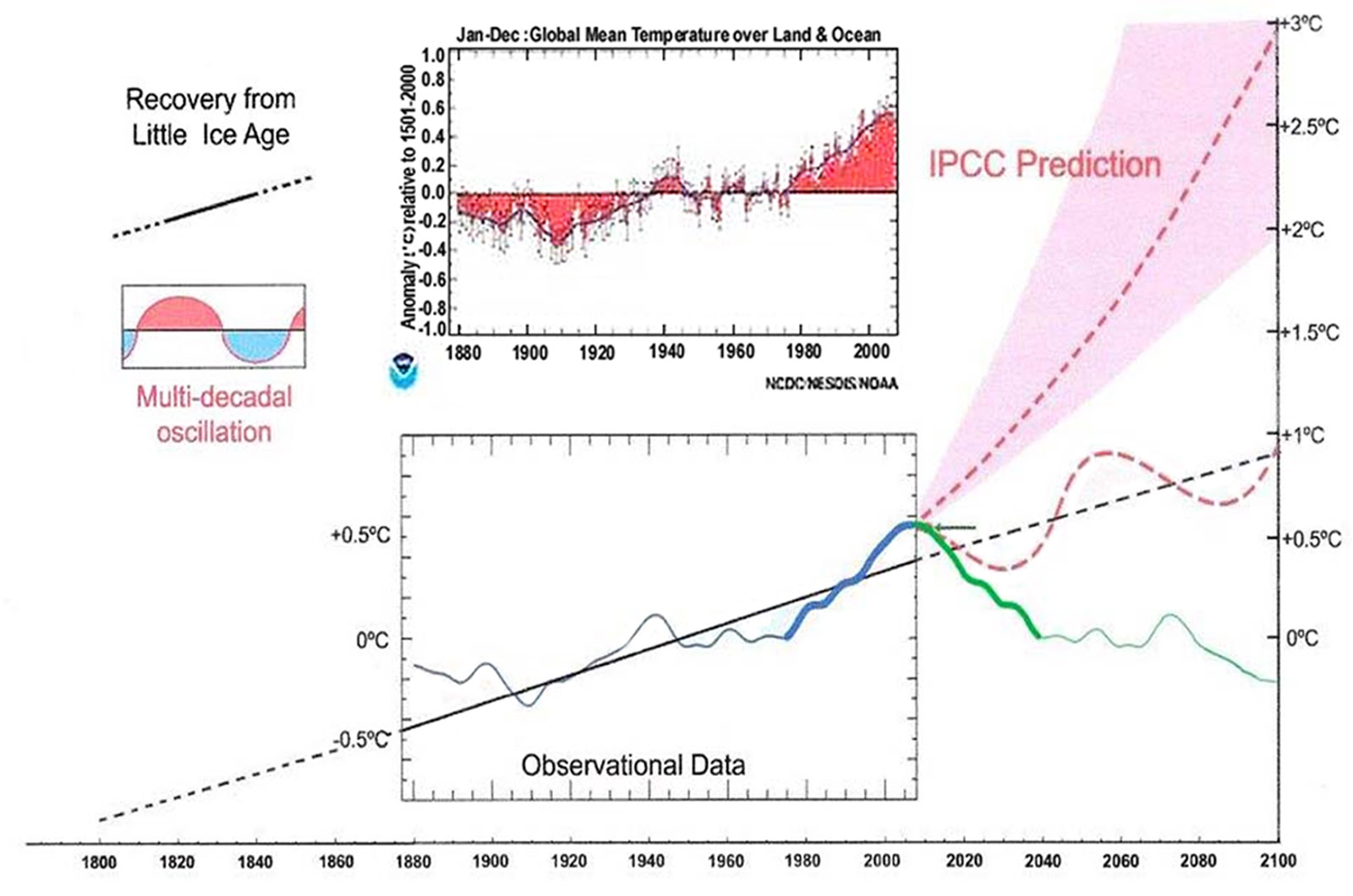

http://www.climatedepot.com/2018/01/26/analysis-the-coming-cooling-sea-surface-temp-data-confirms-cooling-is-on-the-way/
They make the two fatal schoolboy errors of first, using too small (short) a sample size ie ignoring the millennial cycle and using only 50 – 150 years of data and second of projecting straight ahead across the 2004/5 millennial peak and trend inversion
Fig. 12. Comparative Temperature Forecasts to 2100.
Fig. 12 compares the IPCC forecast with the Akasofu (31) forecast (red harmonic) and with the simple and most reasonable working hypothesis of this paper (green line) that the “Golden Spike” temperature peak at about 2003 is the most recent peak in the millennial cycle. Akasofu forecasts a further temperature increase to 2100 to be 0.5°C ± 0.2C, rather than 4.0 C +/- 2.0C predicted by the IPCC. but this interpretation ignores the Millennial inflexion point at 2004. Fig. 12 shows that the well documented 60-year temperature cycle coincidentally also peaks at about 2003.Looking at the shorter 60+/- year wavelength modulation of the millennial trend, the most straightforward hypothesis is that the cooling trends from 2003 forward will simply be a mirror image of the recent rising trends. This is illustrated by the green curve in Fig. 12, which shows cooling until 2038, slight warming to 2073 and then cooling to the end of the century, by which time almost all of the 20th century warming will have been reversed.
Here is Orssengo’s version -which is very similar to Akasofu
Orssengo is better than most in that he has amazingly discovered the 60 year cycle !! The establishment remain blind to the obvious millennial cycle.
I was wrong in this figure because I did not realise then that the secular GMT is quadratic, not linear.
Haven’t read all the comments, so I may be repeating what soemone else has said. If so, apologies.
Girma quotes Wu et al 2011 as having determined the secular rate of warming by subtracting the 55-70 year MDO form “observed” GMT. As if that were the only periodicity in GMT. Oh, come on, please.
Anyone who’s looked at ice core paleotemperature reconstructions can see (no fancy fourier analysis needed, just eyeballs) that there’s a roughly 1,000 year cycle. That’s why we talk of the Medieval, Roman and Minoan Warm Periods.
We’re close to the top of a 1,000 year cycle now (assuming that it is a cycle and is continuing).
So, how do you distinguish, in 120 years of data, between a secular variation and being on the up-slope of a 1,000 year cycle. You can’t. It’s just not possible.
Also, the premise that all changes in GMT are due to CO2 is totally unjustified. It appears that the only “justification” is a set of models that were written assuming that CO2 is the only driver of temperature.
And I haven’t mentioned the dreaded “adjustments” yet. No need. Girma’s otherwise fairly rigorous analysis is based on two very flawed assumptions.
I agree with the “Smart”,
Mr. Smart Rock:
Just wanted to add
the “1,000” year cycles
from ice cores
are really more like
1,000 years +/- 500 years.
Not as precise as you imply.
If you take unadjusted data from NOAA, apply a 1.2TCS CO2, a small solar input, small aerosol input, and a 0.23C variation from PDO/AMO with a 60 year period. You can simulate the entire historical record with almost zero error from 1880 to now. Using corrected data produces a horrible fit. I couldn’t get any value of TCS or other parameters to produce a good fit.
The way you have calculated this is the only way you can do it with any scientific legitimacy. The 70 year period from 1945-2015 shows a 0.4C change which is consistent as well with a TCS ~ 1.2. To suggest 2.2-2.8 as a recent paper suggested means that somehow over the last 70 years heat has been lost or stored in the system
Yes….Trenberth’s Lament, the missing heat.
The climate change religion is lost in the wilderness, stranded by the obviousness of the failure of their cherished hypothesis. The climate alarmism cult is unable to cope with the fact that anthropogenic CO2 is a complete non-problem.
nologic nologic nologic
What “unadjusted data” from NAAO?
What are you drinking?
Very few southern hemisphere
measurements before 1900.
Few southern hemisphere
measurements from 1900 to 1940.
Over half the grids, even today,
have no measurements.
So, a large majority of our planet’s surface
before 1940 had no measurements,
.
So, a majority of our planet’s surface
after 1940 had no measurements.
Substitute the phrase “no data”
for “no measurements”.
The majority of the average surface
temperature compilation
is derived from wild guess numbers
from government bureaucrats
who want to show more warming!
So, even if you could get
“real raw data”
from NAAO,
which I doubt,
a majority of the numbers
would still be wild guess infilling,
and wild guess infilling,
especially by biased bureaucrats
is not real scientific data.
Wow. What rigor. Mortis.
Doesn’t temperature lead, by a decade, the historical increase in CO2?
No. Per ice cores, it leads by ~800 years, the thermohaline circulation round trip. Makes sense.
ristvan,
Depends of the depth and speed of the change and the processes involved…
Seasonal: 2-3 months (vegetation dominant), CO2 opposite to temperature
Year by year: 6 months (vegetation dominant), CO2 parallel to temperature
MWP-LIA and other millennials: decades (ocean -surface- currents?), CO2 parallel to temperature
Glacial-interglacial: centuries to millennia (deep oceans), CO2 parallel to temperature
“Using the mathematical model given by Eq. 3, if for a given middle year of a trend period, the GMT trend dT/dy and the relative atmospheric carbon dioxide trend (dC/dy)/C are known, the CO2 doubling GMT T2x could be estimated directly [from] observations.“.
No it couldn’t. The statement assumes that temperature (GMT-MDO) is driven solely by CO2.
It is just, that the global warming target of +2°C, or only +1.5 is from “pre-industrial” averages, whatever that means. With the claim, that temperatures had already increased by over 1°C, the “threat” is immanent and will not require additional evaluation.
Rather than the consequences of a further doubling of CO2, we could question the requirements for it. Natural CO2 sinks consume about 2% of elevated atmospheric CO2 levels every year. These are about 20Gt right now, with a concentration of about 405ppm.
To eventually get to (in the long run) and maintain a level of 800ppm, it would require (800-280)*0.02 =10.4ppm of CO2 emissions per year, or 81Gt of CO2. So we would need to double CO2 emissions, and then wait a long time (while holding emissions steady) to ever get to 800ppm.
I don’t say it is impossible, but would it take a huge effort by going into the “wrong” direction.
Since satellite measurement of global CO2 reveals that the highest concentrations of CO2 are in the areas of most intense vegetation then increased global vegetation caused by warming probably accounts for the increased global CO2.
Bill Everett,
Would be difficult as the biosphere is a proven, growing sink for CO2, based on the extra O2 produced: the calculated O2 use from burning fossil fuels is more than what is measured as O2 loss in the atmosphere, thus plants produce more O2, thus take more CO2 out of the atmosphere by photosynthesis…
Ferdinand,
You have to ignore the OCO-2 data to still hold that belief. A decade of OCO-2 data will smash your existing paradigms of where the sources and sinks are.
joelobryan,
My impression is that the OCO-2 satellite still has a lot of problems, like a maximum CO2 level at the exact place where the maximum uptake of CO2 into the deep oceans is: the N.E. Atlantic, the main sink place for the THC. I suppose that it is because of these problems that we haven’t seen any updates in the past year…
This article assumes that the only natural cause of climate change are ocean related occilations. If that is so them we should never had the ice age cycling or the warm period, cool period cycling during the Holocene but we did. The primary flaw in the AGW conjecture is that it is based on only partial science.
That makes no sense because vegetation growth is a sink.
(Above post responding to Bill Everett)
Oh boy, another smooth curve analysis of a chaotic, non-linear system. And to top it off, we ignore the last nine years. Wouldn’t want those nasty, ugly impulses in 2010 and 2016 to ruin our pretty lines.