Guest essay by Dr. Antero Ollila
WUWT previously published my essay on the Semi Empirical Climate Model’ on the 21st of November. In that essay I used the term “IPCC climate model” and I received some comments saying that the “IPCC has no climate model”. I understand this argument, because IPCC should not have any models according to its mission statement.
In this essay I analyze in detail the evidence of the IPCC climate model, its properties, and its usefulness in calculating the warming values according to the IPCC science. I reckon that some readers shall also argue that there is no such thing as “IPCC science”. The mission statement says role of the IPCC…
“…is to assess on a comprehensive, objective, open and transparent basis the scientific, technical and socio-economic information relevant to understanding the scientific basis of risk of human-induced climate change, its potential impacts and options for adaptation and mitigation. IPCC reports should be neutral with respect to policy, although they may need to deal objectively with scientific, technical and socio-economic factors relevant to the application of particular policies.”
The mission statement above guides IPCC to concentrate to assess human-induced climate change issues and it means that the natural causes have a bystander role. IPCC must summarize the assessment results and to compose concise presentations based on the thousands of scientific papers. The outcomes of this work can be found in the IPCC’s reports. Finally, we have presentations like Radiative Forcings (RF) of greenhouse gases, Transient Climate Sensitivity (TCS), and Equilibrium CS (ECS). The IPCC has composed these presentations based on few scientific papers or even on its own task forces like in the case of Representative Concentration Pathways (RCPs). Therefore, it is justified to call this work “IPCC science”. It is not typically based on any individual scientific work alone, but it is based selections and combination work of IPCC.
It is true that the IPCC does not openly manifest that “this is the IPCC simple climate model”, because it would be clearly against its mission. But, it can be found in the IPCC Assessment Reports. I refer to 3rd, 4th, and 5th Assessments Reports using the acronyms TAR, AR4, and AR5. The oldest reference to the IPCC climate model can be found in TAR, chapter 6.2.1:
The climate sensitivity parameter (global mean surface temperature response dTs to the radiative forcing dF) is defined as (I have changed the Greek symbols into English ones). Equation 6.1:
dTs /dF = CSP
(Dickinson, 1982; WMO, 1986; Cess et al., 1993).
Equation 6.1 is defined for the transition of the surface-troposphere system from one equilibrium state to another in response to an externally imposed radiative perturbation. In the one-dimensional radiative convective models, wherein the concept was first initiated, CSP is a nearly invariant parameter (typically, about 0.5 K/(Wm−2); Ramanathan et al., 1985) for a variety of radiative forcings, thus introducing the notion of a possible universality of the relationship between forcing and response.
The same equation can be found chapter 2.2 of AR4 and on page 664 of AR5 in the form of equation 1 below
dT = CSP * RF
…where RF means Radiative Forcing.
The value of CSP is 0.5 K/(W/m2) according to TAR, and there is reference to the paper of Ramanathan et al. (1985). I read this paper, and I found Table 8, in which eight CSP values are tabulated from 0.47 to 0.53. One of the values was that of Ramanthan et al., and it is 0.52. The average value of these eight CSPs is 0.5. So, it looks like that the reference of TAR is not accurate. The oldest reference is to the paper of Wanabe & Wetherald (1967) and it may be the oldest reference to equation 1.
Another essential equation in the IPCC climate model is the RF formula by Myhre et al. (1989) for carbon dioxide (CO2) is equation 2 below
RF = k * ln (CO2/280)
where k is 5.35 and CO2 is the CO2 concentration (ppm). IPCC selected this equation bases on the assessment in TAR, section 6.3.5. The closest rivals were the equations of Hansen et al. and Shi. IPCC has calculated the CO2 forcing in the AR5 according to equation (2) (AR5, p. 676). The RF value of CO2 concentration of 560 ppm according to equation 2 is 3.7 W/m2. In Table 9.5 of AR5 is tabulated the same 560 ppm RF values of 30 AOGCMs (Atmosphere-Ocean Global Circulation Model also known as ‘coupled atmosphere-ocean models’), and the average value is 3.7 W/m2. It is well-known that equation (2) has been commonly used practically in all GCMs, and probably that is why Gavin Schmidt et al. (2010) calls it a “canonical estimate”.
IPCC describes its equation 6.1 like this:
Equation (6.1) is defined for the transition of the surface-troposphere system from one equilibrium state to another in response to an externally imposed radiative perturbation.
The word “equilibrium” is not a proper expression for this equation, because it could mean that this equation is applicable only for equilibrium states as defined by the specification of ECS. The basic difference between the TCS and ECS is in the positive feedbacks.
In AR5 chapter 12.4.5.1, Atmospheric Humidity there is this text:
“A common experience from past modelling studies is that relative humidity (RH) remains approximately constant on climatological time scales and planetary space scales, implying a strong constraint by the Clausius–Clapeyron relationship on how specific humidity will change.”
It is well-known that all IPCC referred climate models apply the positive water feedback and it is inherently in the value of CSP, if the value is 0.5 K/(W/m2) or greater. In ECS calculations also other positive feedbacks are taken into account like the snow and ice albedo decrease.
IPCC summarizes the differences of ECS and TCR (IPCC has changed the term TCS to TCR (Transient Climate Response)) in AR5 like this (page 1110):
“ECS determines the eventual warming in response to stabilization of atmospheric composition on multi-century time scales, while TCR determines the warming expected at a given time following any steady increase in forcing over a 50- to 100-year time scale.”
And further on page 1112, IPCC states that “TCR is a more informative indicator of future climate than ECS”. I will show later that all the IPCC calculations for future scenarios for this century are based on the TCS/TCR approach, i.e. only the positive water feedback has been applied.
In Table 9.5 are the average values of ECS and TCR of 30 AOGCMs and the values are 3.2 C and 1.8 C. According to equation 1 it is impossible to get ECS value of 3.2 K by multiplying the RF value of 3.7 W/m2 by the CSP value of 0.5 K/(W/m2) as the explanation by IPCC could insist. In Table 9.5 the average CSP is 1.0 for calculating the ECS value. The TCR value calculated according to equation 1 would be 0.5 * 3.7 = 1.85 K, which is practically the same as the average value of 30 AOGCMs. My conclusion is this: the expression “one equilibrium state to another” for equation 1 and the CSP value of 0.5 K/(W/m2) does not mean the equilibrium between the equilibrium climate sensitivity (ECS) states but equilibrium states according to TCR calculations.
We can combine equations 1 and 2 into one formula (equation 3) for CO2
dTs = CSP * k * ln(CO2/280)
If the CSP value is 0.5 K/(W/m2) and the k = 5.35, I call equation 3 the IPCC climate model. Equation 3 cannot be found in any original research paper. If somebody can do so, then I will change my mind.
IPCC has carried out the following selections:
- The elements of the equations
- The value of CSP is 0.5 K/(W/m2) (IPCC’s own value, not Ramanathan et al.)
- The RF formula for CO2 forcing.
IPCC has carried out scientific work by assessing the original research papers and selecting the elements for its model. I have done the same thing. My selection for the model elements is the same but the value of CSP is 0.27 K/(W/m2) and the value of parameter k is 3.12. It is a common practice to call my model the Ollila’s climate model and in the same way we can call the selections of IPCC to be IPCC climate model.
Even though equation 1 is as simple as possible, it is very good and accurate expression about the dependency of the surface temperature change needed to compensate the decrease of the outgoing longwave radiation (OLR) at the top of the atmosphere (TOA) originally caused by the increased absorption of CO2 concentration increase. The evidence is shown in Figure 1.

I have calculated the OLR changes using the spectral calculations applying the average global atmospheric conditions for three CO2 concentrations namely 393, 560 and 1370 ppm. There is no model applied in these calculations except the complicated absorption, emission, and transmission equations of the LW radiation emitted by the Earth’s surface in the real atmospheric conditions.
The dependency between RF change and the surface temperature change is essentially linear. This can be noticed by comparing the red curve calculated using the CSP value of 0.27 k(W/m2) to the blue curve of the spectral calculations. The TCS/TCR value of 0.6 C degrees can be read directly from Figure 1.
As shown above, the TCS/TCRds value of 1.8…1.9 C degrees is the same calculated by the IPCC’s climate model or by the AOGCMs. The warming values of RCP scenarios are originally calculated by the AOGCMs as well. IPCC tries to muddle the water by calculating the warming values of RCPs from the period 1986-2005 to the period 2081-2100, and not for the period 1750-2100 what is the specification of RCPs:
“The RCPs are named according to radiative forcing target level for 2100. The radiative forcing estimates are based on the forcing of greenhouse gases and other forcing agents. The forcing levels are relative to pre-industrial values and do not include land use (albedo), dust, or nitrate aerosol forcing.”
The warming of RCP8.5 for this period is 3.7 C degrees according to AR5 time span above. The warming from 1750 to 2000 has been 0.6 C degrees per IPCC. Thus, the total warming according to the RCP original specification from 1750 to 2100 is about 0.6 + 3.7 = 4.3 C degrees. Applying the IPCC’s climate model, the result is 0.5 * 8.5 = 4.25 C degrees, which is close enough.
The dependency between the CO2 concentration and the RF value is: RF = k * ln(CO2/280), where k is 3.12, In Figure 2, note that the equation starts from the CO2 concentration of 280 ppm onward, where the curve is slightly non-linear.

Usually I do not approve of the essential results of IPCC, but I do approve of this statement found in Chapter 6.2.1 in TAR:
“The invariance of CSP has made the radiative forcing concept appealing as a convenient measure to estimate the global, annual mean surface temperature response, without taking the recourse to actually run and analyse, say, a three-dimensional atmosphere-ocean general circulation model (AOGCM) simulation.”
Using equations (1) and (2) it is easy to calculate the TCS/TCR values (ECS values are not needed during this century and they are not real anyway) and the temperature effects of RCPs. For example, the temperature effect of RCP8.5 according to IPCC in 2100 is simply 0.5*8.5 = 4.25 C degrees, because the number 8.5 means RF value in 2100. The RF value of 8.5 W/m2 corresponds to the CO2 concentration of 1370 ppm, and according to my model the warming impact would be only 1.3 C. Eq. (1) is applicable for warming calculations, if a RF value is known. The RF values of GH gases can be calculated by equation 2, if equivalent CO2 values are known. But I do not recommend the CSP and k values of IPCC.
Why IPCC does not openly show that they have this simple climate model, which is very easy to apply, and which gives the same results as very complicated AOGCMs?
One reason could be that they are little bit shy to call it IPCC model, because they should not have it. Another reason could be that openly using it would decrease the image of climate change science, if it turns out that actually AOGCMs are not needed for calculating global warming values, which are very important in the tool box of IPCC.
There is a supposition that it is an unwritten rule among the climate change scientists that the values of the IPCC model and average GCMs should give essentially the same global values. The facts show that this is the case.
[QUOTE FROM POST]In AR5 chapter 12.4.5.1, Atmospheric Humidity there is this text:
“A common experience from past modelling studies is that relative humidity (RH) remains approximately constant on climatological time scales and planetary space scales, implying a strong constraint by the Clausius–Clapeyron relationship on how specific humidity will change.”
An assumption of constant relative humidity is a flawed assumption for calculating the warming due to an increase in IR absorption due to higher CO2 concentrations. The Clausius-Clapeyron equation is basically a theoretical curve-fit of the vapor pressure of a liquid as a function of temperature over a narrow temperature range, expressed as
dPv/d(1/T) = -Hv/R
where Pv represents the vapor pressure of a liquid at an absolute temperature T (in Kelvin), Hv is the heat of vaporization of the liquid, and R is the ideal-gas constant. Since the heat of vaporization varies with temperature, for most liquids we can get a more accurate curve-fit using the Antoine equation
Pv = exp[ A – B/(T+C)]
where A, B, and C are constants for a given liquid.
For air in equilibrium with a body of liquid water, the mole fraction water vapor in the air at 100% relative humidity is given by
y = Pv(T) / Pa
where Pv is the vapor pressure of water at temperature T, and Pa is atmospheric pressure. Since the vapor pressure Pv(T) increases with temperature, the mole fraction of water at 100% RH increases with temperature (warm air can hold more water vapor than cold air). If the relative humidity is assumed constant when the air is warmed, the warmer air contains more water vapor than the cooler air.
If the IPCC model assumes constant relative humidity while the air is being warmed by absorption of IR radiation, the additional water vapor in the atmosphere must come from somewhere. Since the Earth’s surface is 70% covered by water, this can come from evaporation of liquid water, but evaporation of water requires the air to supply about 580 calories of heat per gram of water evaporated.
Depending on the assumed original temperature of the air, heat required to evaporate water to maintain constant relative humidity can consume about 50 to 70% of the heat used to warm the air, meaning that “constant relative humidity” is a negative feedback with a coefficient of -0.5 to -0.7 on the temperature response to 1 W/m2 of IR radiation absorbed.
The IPCC is eager to claim “credit” for additional water vapor in the atmosphere for its ability to absorb more IR radiation, and supposedly amplify the CO2 effect, but they neglect the strong negative feedback of the heat required to evaporate the water.
To Steve Zell. There is something wrong in the assumption of the constant relative humidity, because it can be found only in the short-term events liken El Nino / La Nina but not in the long-term changes, see my figure on the issue. I have not found any explanation, why the atmosphere prefers the constant absolute humidity.
“If the IPCC model assumes constant relative humidity”
Goodness knows what model is now being assigned to the IPCC. There is no humidity in Dr Ollila’s. But this is a frequent distortion of the quote given
“A common experience from past modelling studies is that relative humidity (RH) remains approximately constant on climatological time scales and planetary space scales”
It is “common experience”, not an assumption. GCMs do not make global assumptions of that kind. They can’t. What they do do is to conserve mass.
Yes Nick. I agree that in GCMs they do not assume the constant relative humidity but the physical relationships show that it remains approximately constant. That is correct, and my expression was wrong. In the end, we should notice that the real atmosphere works in that way but it does not. I have calculated theoretically in two ways that the absolute water content of the atmosphere is constant. Also the direct measurements support this result not the constant relative humidity.
Link: http://www.seipub.org/DES/MostDownloaded.aspx
“…but the physical relationships show that it remains approximately constant”
But not during cloud formation which arises from air that is supersaturated with water vapour. A very non-trivial inconvenience.
The local time is now 23:09. I will come back after 10 hours and to check, if there are any new comments.
I have to apologize in advance, because I have not read and checked all comments in this blog post,and also I may be in complete misunderstanding of this blog post….but for what it could be worth……the below equation, for as far as I can tell is what I will call a paradoxical one,which lacks relevance and meaning
dT = CSP * RF
Considering dT in relation to a constant value like Rf in that equation turns all the meaning in that equation to a paradox…
That equation consist in principle as a runway warming one, but that is not the main point with it, the main point is the use of the RF value in that equation, which happens to be not a variable, when dT still a variable.
In principle the equation still will be a runway warming equation but not a paradoxical one, if RF in that one equation is swapped for dRF…..
dRF is not the same as RF……and it changes the point of that equation to a non paradoxical one.
In principle dRF= RFa -RFi where “a” in RF stands for the actual value of RF as per the actual value of the CO2 ppm concentration considered in calculating, and “i” in the RF stands for the RF initial point as per ppm initial point in consideration of CO2 ppm initial point for the equation and its calculations.
So if RF= blah..blah ( CO2/280)
dRF= blah..blah ((CO2a – CO2i)/CO2m) where “m” stands for the value CO2 as the CO2 mean…….
So for example trying to get the dRf for an actual 380 ppm point, from a starting point of 280 ppm with a supposed mean of 260 ppm, then the
dRF= blah..blah ((380 – 280) / 260)….
Now what the numbers for dT will be if dRF used instead of RF in this context????
And the main point in this is that dRF in that equation still as far as this does have some value, still it does not move that equation out of its runway warming tendency, but at the very least will make it workable and not paradoxical…
dT is not actually compatible as for and in that IPCC equation, or model, with the RF……..as far as I can tell.
And maybe I just simply being wrong with this, but hey…..please, who ever can assist and show me my wrong in this please do…. simply trying to expand my understanding.
cheers
In a way you right the the RF value referred in this equation is actually the dRF value, which has been calculated from the steady-state situation in year 1750. Because all GH gas concentrations have been increasingsince 1750, the RF value in comparison to the year 1750 have been increasing. The RF values are the used in my story in the same way as IPCC uses them. They simply marked them as RF even though they are changes from the year 1750 value.
aveollila
December 12, 2017 at 5:59 pm
Thanks for the consideration and the reply to me, aveollila.
Still there is no equality to be considered in between RF and dRF.
The “d” changes it and could not permit it, the parameter of variation…..the “d” thingy…will block an equality, or equalization between RF and dRF,as per the equation….
As I said, the equation as per my approach still not correct one at that point, but still not paradoxical,
You some how consider an equation where there the RF is straight forward given in a proper RF meaning and you still somehow strangely enough consider it as a dRF…
That in principle it can not be.
If it is RF, then it can not be considered as dRF…because this two are not the same thing……but hey in an AGWers world worms do fly…..
And as far as the dT equation stands for the IPCC point is still paradoxical..
Introducing the tester, the timer, the dt, where “t” the time, for same RF there will be different values of dT, very paradoxical as far as I can tell………That will be true for any RF value according to that IPCC equation….
dT= blah x RF x dt will give different values for dT for the same and in relation to the same value of RF in all possible ranges of RF considered,,,, a paradox…. for lack of better word…..
I am sure this is not very helpful at this point….but still…
cheers
In the original post Fig 2 is misleading, the green line representing CO2 should start at (280,0) also N2O is nitrous oxide not nitrogen oxide which could cause confusion.
Also this graph is deceptive when plotted in terms of wavelength, should be vs wavenumber (proportional to energy).
Much is wrong with Fig 2. The ranges are silly. N₂O and CH₄ are shown in ppm, with the red dot showing that they are currently on the zero axis. They will continue to stay there (in ppm); the curves are meaningless. And wrong; both (per ppm) are stronger GHGs than CO₂. And there is the question of the y axis – temperature change relative to what? For CO₂ it is at zero concentration. But for a log curve, that should go to -∞.
You are right that curves could start from 280 ppm. Anyway, the actual CO2 concentrations have been a long time over 280 ppm and therefore it has no practical meaning.
The expression of nitrogen oxide is not a specific enough and you are right, therfore, nitrous oxide is the right expression.Thanks for these corrections.
Climate models don’t work, because none account for North Korea’s glorious leader’s ability to control the weather:
http://www.smh.com.au/world/kim-jongun-controls-the-weather-north-koreans-told-20171212-h030w3.html
I found it always strange how climate scientists consider the average temperature of the Earth being given only by the atmosphere, ignoring completely the oceans in this calculation.
It is well known that the continental climate is different and colder to the climate around seas.
Attributing all the warming to the atmosphere and ignoring the oceans is an error.
“Attributing all the warming to the atmosphere and ignoring the oceans is an error.”
AOGCMs don’t do that.
“AOGCMs don’t do that.”
All warming is considered to come from the atmosphere – as explained above:
“Just briefly about CO2 and GH effect. The GH effect is real and it matches well with many scientific calculations methods. IPCC does not want to address the contribution of CO2, because they know that the most referred value 26 % of Kiehl & Trenberth …”
The oceans (water) intake heat differently to a solid object, in a way similar to a condensed atmosphere with its own GH effect. This is not modelled or taken into account to estimate why the average surface temperature is increased from 255K to 288K.
Because the ocean cover about 70 % of the Earth’s area, they have this much influence in calcuating the average surface global temperatures.
Exactly. And what is the difference between the average ocean temperature in comparison with the average land surface temperature not considering the atmosphere?
The fundamental assumption at the base of the climate consensus view is that blocking of radiated energy by radiative (greenhouse) gasses is the only factor raising the Earth’s mean surface temperatures to current levels. For the past decade, at least, there has been an alternative explanation in the thermal buffering provided by our atmosphere and ground over the daily temperature cycle.
This can be seen most simply in the DIVINER temperature data for the moon. Rather than dropping to around -270 C near the absolute zero of space, as it would if the surface was a perfect thermal insulator, it drops to around -150 C at sunset then slowly down to below -270 C over the lunar night as the ground cools. During the day it rises to around 100 C, or lower than it would if the surface wasn’t absorbing heat.
Due to the nonlinear relationship between radiated energy and temperature, E = aT^4, a temperature drop of, say, 1C during the day drops radiated energy far more than the same increase in temperature increases radiation at night. The mean surface temperature rises to regain radiative balance over the daily cycle. This is basic undergraduate physics and simple spreadsheet models give good agreement with observation.
Calculation for the Earth is more complex due to the varying nature of our surface, but simple calculations show that this effect, alone, is capable of fully accounting for our suface temperatures.
Because the GHE is not the only game in town, the original assumption needs justification. To remain plausible and scientifically valid it needs quantification. Those supporting the IPCC position need to show that the buffering effect is less than 1% of the generally accepted values of 60-100 C, and that the GHE is 200 times greater than the 0.14 C I calculate it to be.
dai
actually, “Those supporting the IPCC position” start with a non rotating and non tilting, perfectly homogeneous and flat Earth, which receive everywhere ~240 W/m² after albedo. So the buffer effect is already computed in the reference temperature 255K corresponding to these 240 W/m².
As you pertinently point out, the average temperature would be lower if the reference were alternate 480 W in day and 0 W in night.
What they miss is the fact that the atmosphere keeps the surface WARMER than a perfect insulator would (back-radiation exceed the primary solar heating, which a perfect insulator cannot do). Insulating properties do not account for that. A heat pump is needed for this to happen.
dT = CSP * RF …
is a linear equation in a system well known NOT being linear. T is known to vary with ENSO (just for instance, but many other things also come into play the same way) without any forcing.
Use it “back of envelope” is fine, just to figure out if it is worth caring.
Use it in models, however, is malpractice incarnate.
It isn’t a linear equation, unless CSP is constant, which they don’t specify. It’s a definition for CSP. And it isn’t used in models.
play-words, as usual with you.
The reference by aveollila (12/12/2017 @7:43 am) to the reality of the greenhouse effect (GHE) is irrelevant to the IPCC climate mode, the subject of his essay. IPCC divides GHE, whether real or fictional, in two: a natural part it considers to be in equilibrium, plus an enhanced part caused by human CO2 emissions modeled to produce catastrophic warming a century in the future. Both violate physics (nothing in climate is in equilibrium, [CO2] is controlled by Henry’s Law and [H2O] by the Clausius-Clapeyron Relation), but while violating physics might frustrate IPCC climatologists, in the final analysis it matters no more than the fact that its model has zero predictive power. Neither species of science, MS nor PMS, requires fidelity between models and physics or any other models: PMS requires intersubjective testing but no empirical testing, while MS requires objective testing plus fidelity to all relevant data, but nothing subjective. The two species of science are orthogonal.
Secondly, aveollila’s claim that the GH effect … matches well with many scientific calculations is peculiar on several counts. The various definitions of GHE provide nothing specific to measure. GHE accounts for the insulation provided by the atmosphere, the blanket effect, making it a consequence of infrared radiation absorption by the component gases. GHE applies to a thin blanket as well as a thick one. GHE provides no estimate of the effective thickness of the blanket, the temperature drop across the blanket anywhere, or the gas composition of the atmosphere. GHE does not specify which variables are dependent or which are independent, which are cause and which are effect. In short, the GHE is an accounting for measurements; it is not a thing to be measured.
The GHE is, of course, real. It is a vital radiation link in the thermodynamic model of the climate of a planet warmed by its sun. GHE is not sufficient, however, to estimate the surface temperature. That is precisely what IPCC attempts to do with its Radiative Forcing paradigm, which it regularly defends against unnamed and apparently unpublished (of course) critics. E.g., AR5, Ch. 8, Anthropogenic and Natural Radiative Forcing, Executive Summary, p. 8; AR4, §2.8 Utility of Radiative Forcing, p. 195. TAR, Ch. 6, Radiative Forcing of Climate Change, Executive Summary, p. 351.
IPCC’s model problems lie elsewhere than in the reality of GHE. IPCC’s model begins by holding Earth’s albedo constant, when instead it varies with global average surface temperature (GAST). And IPCC’s model then enhances the GHE by making atmospheric CO2 increase in proportion to the total of human CO2 emissions, when instead the ocean regulates the total atmospheric CO2 concentration, also in proportion to GAST. The first of these GAST feedback mechanisms mitigates temperature change from any cause, counteracting both the natural and the enhanced GHE. Because cloud albedo gates the Sun on and off, it is the most powerful feedback in climate, one again missing from the IPCC model. The second missing feedback mitigates against any CO2 emissions, natural or manmade. It removes any enhanced GHE by making atmospheric CO2 concentration an effect of surface temperature rather than a cause. Small wonder that the IPCC model doesn’t work.
aveolila (12/12/17 @ur momisugly 8:06 am) claims There are more than 100 GCMs and they all are different in some degree. The major differences are in the amount of positive feedbacks. The result can be seen in the so-called spaghetti diagrams.
Q. What do you call the composite of 100 GCMs? A. A GCM.
Q. When is the composite of a lot of samples better than a single sample? A. When the samples are independent.
Q. Why is the composite of 100 GCMs no better than any one of them? A. Because IPCC has formally doctored the data into conformance with its presumption in its revised charter that anthropogenic climate change exists:
• AeroCom: Aerosol Model Intercomparison
• AMIP: Atmospheric Model Intercomparison Project
• CMIP: Coupled Model Imtercomparison Project
• MIP: Model Intercomparison Project
• PCMDI: Program for Climate Model Diagnosis and Intercomparison
• PMIP: Paleoclimate Modelling Intercomparison Project
• RTMIP: Radiative-Transfer Model Intercomparison Project
• TransCom 3: Atmospheric Tracer Transport Model Intercomparison Project
Plus these to some degree:
• GISP2 Greenland Ice Sheet Project 2
• GLODAP Global Ocean Data Analysis Project
• GPCP Global Precipitation Climatology Project
• GRIP Greenland Ice Core Project
• ISCCP International Satellite Cloud Climatology Project
• NVAP NASA Water Vapor Project
All as of AR4, Climate Change 2007.
As for spaghetti graphs, IPCC provides a remarkable example as a cover-up for its adoption of Mann’s 1999 Hockey Stick. IPCC bought the Hockey Stick in 2001. TAR, Summary for Policymakers, Figure 1(b), p. 3. http://www.ipcc.ch/ipccreports/tar/wg1/images/figspm-1s.gif
Following McIntyre & McKitrick’s 2003 debunking of the Hockey Stick, IPCC rather than retract its position, obfuscated its choice by embedding it in a spaghetti graph comprising 13 model results. AR4, §6.6.1.1, What Do Reconstructions Based on Palaeoclimatic Proxies Show? pp. 466-7, Figure 6.10(b).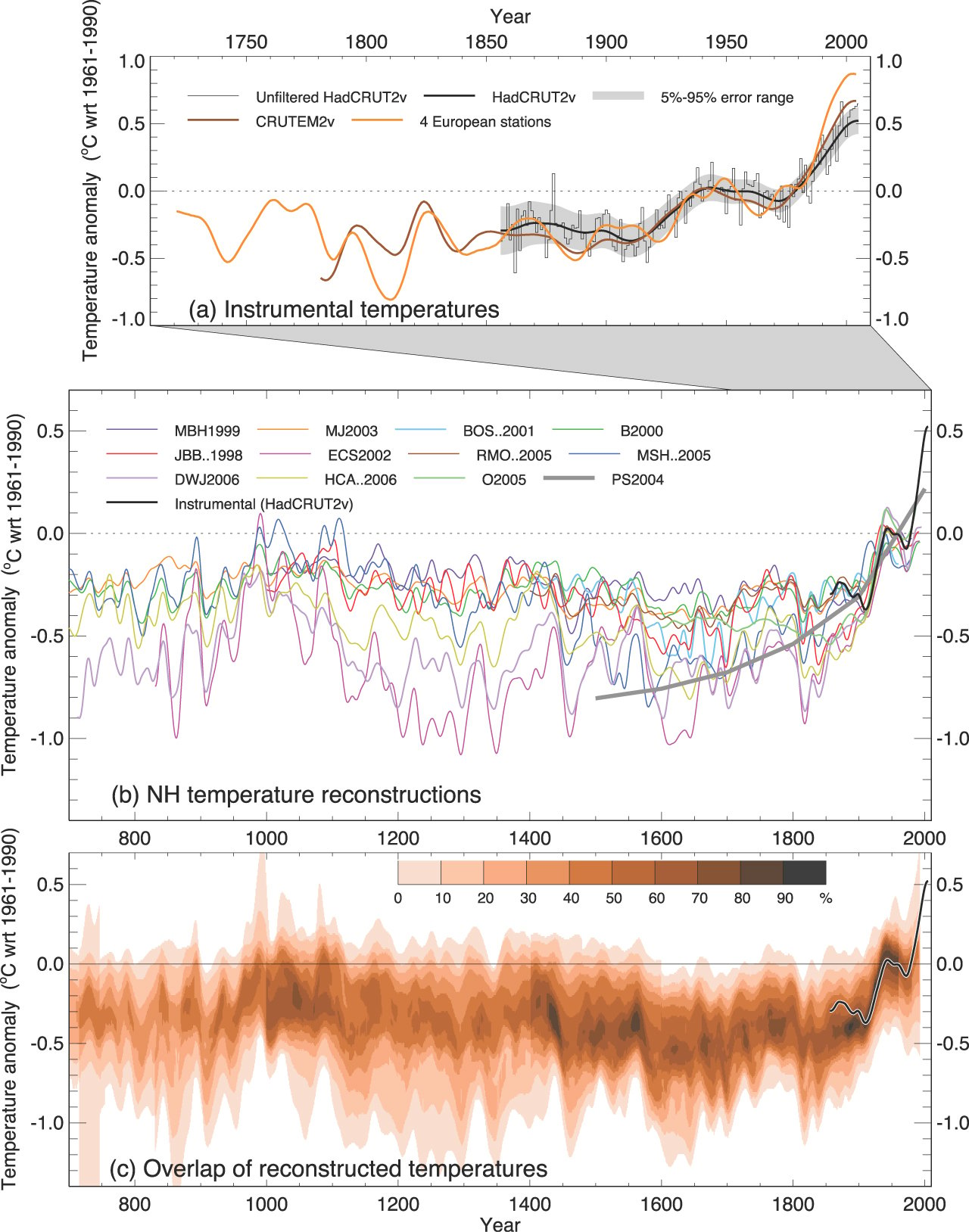
And Lo & Behold! All the reconstructions look like Hockey Sticks! Mann is rehabilitated. The reason is plain: following Mann’s methods, IPCC and the authors French-curved the data from the added reconstructions to blend the various temperature proxies into the HadCRUT2v version of the modern instrument record.
Data from biological, hydrological, and geological sources are effects accumulated over decades to eons, while the data from instrument records are accumulated over seconds to minutes. A sensor in general accumulates matter or energy from its environment into a collection aperture creating what is called a low pass filtered version of the source evolution. The acquisition process attenuates and delays the data record with respect to the input events in proportion to the integration time. As a result, events such as any segment of the temperature record of the instrument era would not even be visible in an ice core record. Appending one unprocessed record to another with a different integration time constant creates a distorted composite record. Then smoothing the transition where the records join further misrepresents the data.
IPCC’s methods here are just a few examples of the many forms of junk science practiced by IPCC. But for the wasted treasury, the political disruption, the resulting human suffering, and the damage to scientific credulity, IPCC is a laughing stock.