Guest essay by Antero Ollila
The error of the IPCC climate model is about 50% in the present time. There are two things that explain this error:
1) There is no positive water feedback in the climate, and 2) The radiative forcing of carbon dioxide is too strong.
I have developed an alternative theory for global warming (Ref. 1), which I call a Semi Empirical Climate Model (SECM). The SECM combines the major forces which have impacts on the global warming namely Greenhouse Gases (GHG), the Total Solar Irradiance (TSI), the Astronomical Harmonic Resonances (AHR), and the Volcanic Eruptions (VE) according to observational impacts.
Temperature Impacts of Total Solar Irradiance (TSI) Changes
GH gas warming effects cannot explain the temperature changes before 1750 like the Little Ice Age (LIA).
Total Solar Irradiance (TSI) changes caused by activity variations of the Sun seem to correlate well with the temperature changes. The TSI changes have been estimated by applying different proxy methods. Lean (Ref. 2) has used sunspot darkening and facular brightening data. Lean’s paper was selected for publication in Geophysical Research Letters “Top 40” edition and it was rewarded.

Lean has introduced a correlation formula between the decadally averaged proxy temperatures and the TSI:
dT = -200.44 + 0.1466*TSI from 1610 to 2000. In my study the selection of century-scale reference periods for TSI changes are selected carefully so that the AHR effect is zero and the forcings of GH gases are eliminated. The Sun causes the rest of the temperature change. The temperature changes of these reference periods caused by the Sun are 0 ⁰C, 0.24 ⁰C and 0.5 ⁰C, which are relatively great and different enough – also practically the same as found by Lean but the correlation is slightly nonlinear (Ref. 1):
dTs = -457777.75 + 671.93304 * TSI – 0.2465316 * TSI2
Nonlinearity is due to the cloudiness dependency on the TSI. This empirical relationship amplifies the direct TSI effect changes by a factor of 4.2. The amplification is due to the cloud forcing caused by the cloudiness change from 69.45 % in 1630s to 66 % in 2000s. A theory that the Sun activity variations modulate Galactic Cosmic Ray (GCR) flux in the atmosphere has been introduced by Svensmark (Ref. 3), which affect the nucleation process of water vapour into water droplets. The result is that the higher TSI value decreases cloudiness, and in this way, there is an amplification in the original TSI change.
Astronomical Harmonic Resonances (AHR) effects
The AHR theory is based on the harmonic oscillations of about 20 and 60 years in the Sun speed around the solar system barycentre (gravity centre of the solar system) caused by Jupiter and Saturn (Scafetta, Ref. 4). The gravitational forces of Jupiter and Saturn move the barycentre in the area, which has the radius of the Sun. The oscillations cause variations in the amount of dust entering the Earth’s atmosphere (Ermakov et al., Ref. 5). The optical measurement of the Infrared Astronomical Satellite (IRAS) revealed in 1983 that the Earth is embedded in a circumsolar toroid ring of dust, Fig. 2. This dust ring co-rotates around the Sun with Earth and it locates from 0.8 AU to 1.3 AU from the Sun. According to Scafetta’s spectral analysis, the peak-to-through amplitude of temperature changes are 0.3 – 0.35 ⁰C. I have found this amplitude to be about 0.34 ⁰C on the empirical basis during the last 80 years.

The space dust can change the cloudiness through the ionization in the same way as the Galactic Cosmic Rays (GCR) can do, Fig.3.

Because both GCR and AHR influence mechanisms work through the same cloudiness change process, their net effects cannot be calculated directly together. I have proposed a theory that during the maximum Sun activity period in the 2000s the AHR effect is also in maximum and during the lowest Sun activity period during the Little Ice Age (LIA) the AHR effect is zero (Ref. 1).
GH gas warming effects
In SCEM, the effects of CO2 have been calculated using the Equation (2)
dTs = 0.27 * 3.12 * ln(CO2/280) (2)
The details of these calculations can be found in this link: https://wattsupwiththat.com/2017/03/17/on-the-reproducibility-of-the-ipccs-climate-sensitivity/
The warming impacts of other methane and nitrogen oxide are also based on spectral analysis calculations.
The summary of temperature effects
I have depicted the various temperature driving forces and the SCEM model calculated values in Fig. 4. Only two volcanic eruptions are included namely Tambora 1815, Krakatoa 1883.

The reference surface temperature is labelled as T-comp. During the time from 1610 to 1880, the T-comp is an average value of three temperature proxy data sets (Ref. 1). From 1880 to 1969 the average of Budyoko (1969) and Hansen (1981) data has been used. The temperature change from 1969 to 1979 is covered by the GISS-2017 data and thereafter by UAH.
In Fig. 5 is depicted the temperatures from 2016 onward are based on four different scenarios, in which the Sun’s insolation decreases from 0 kW to -3 kW in the following 35 years and the CO2 increases 3 ppm yearly.

The Sun’s activity has been decreasing since the latest solar cycles 23 and 24, and a new two dynamo model of the Sun of Shephard et al. (Ref. 6) predicts that its activity approaches the conditions, where the sunspots disappear almost completely during the next two solar cycles like during the Maunder minimum.
The temperature effects of different mechanisms can be summarized as follows:
| Time | Sun | GHGs | AHR | Volcanoes |
| 1700-1800 | 99.5 | 4.6 | -4.0 | 0.0 |
| 1800-1900 | 70.6 | 21.5 | 17.4 | -9.4 |
| 1900-2000 | 72.5 | 30.4 | -2.9 | 0.0 |
| 2015 | 46.2 | 37.3 | 16.6 | 0.0 |
The GHG effects cannot alone explain the temperature changes starting from the LIA. The known TSI variations have a major role in explaining the warming before 1880. There are two warming periods since 1930 and the cycling AHR effects can explain these periods of 60-year intervals. In 2015 the warming impact of GH gases is 37.3 %, when in the IPCC model it is 97.9 %. The SECM explains the temperature changes from 1630 to 2015 with the standard error of 0.09 ⁰C, and the coefficient of determination r2 being 0.90. The temperature increase according to SCEM from 1880 to 2015 is 0.76 ⁰C distributed between the Sun 0.35 ⁰C, the GHGs 0.28 ⁰C (CO2 0.22 ⁰C), and the AHR 0.13 ⁰C.
References
1. Ollila A. Semi empirical model of global warming including cosmic forces, greenhouse gases, and volcanic eruptions. Phys Sc Int J 2017; 15: 1-14.
2. Lean J. Solar Irradiance Reconstruction, IGBP PAGES/World Data Center for Paleoclimatology Data Contribution Series # 2004-035, NOAA/NGDC Paleoclimatology Program, Boulder CO, USA, 2004.
3. Svensmark H. Influence of cosmic rays on earth’s climate. Ph Rev Let 1998; 81: 5027-5030.
4. Scafetta N. Empirical evidence for a celestial origin of the climate oscillations and its implications. J Atmos Sol-Terr Phy 2010; 72: 951-970.
5. Ermakov V, Okhlopkov V, Stozhkov Y, et al. Influence of cosmic rays and cosmic dust on the atmosphere and Earth’s climate. Bull Russ Acad Sc Ph 2009; 73: 434-436.
6. Shepherd SJ, Zharkov SI and Zharkova VV. Prediction of solar activity from solar background magnetic field variations in cycles 21-23. Astrophys J 2014; 795: 46.
The paper is published in Science Domain International:
Semi Empirical Model of Global Warming Including Cosmic Forces, Greenhouse Gases, and Volcanic Eruptions
Antero Ollila
Department of Civil and Environmental Engineering (Emer.), School of Engineering, Aalto University, Espoo, Finland
In this paper, the author describes a semi empirical climate model (SECM) including the major forces which have impacts on the global warming namely Greenhouse Gases (GHG), the Total Solar Irradiance (TSI), the Astronomical Harmonic Resonances (AHR), and the Volcanic Eruptions (VE). The effects of GHGs have been calculated based on the spectral analysis methods. The GHG effects cannot alone explain the temperature changes starting from the Little Ice Age (LIA). The known TSI variations have a major role in explaining the warming before 1880. There are two warming periods since 1930 and the cycling AHR effects can explain these periods of 60 year intervals. The warming mechanisms of TSI and AHR include the cloudiness changes and these quantitative effects are based on empirical temperature changes. The AHR effects depend on the TSI, because their impact mechanisms are proposed to happen through cloudiness changes and TSI amplification mechanism happen in the same way. Two major volcanic eruptions, which can be detected in the global temperature data, are included. The author has reconstructed the global temperature data from 1630 to 2015 utilizing the published temperature estimates for the period 1600 – 1880, and for the period 1880 – 2015 he has used the two measurement based data sets of the 1970s together with two present data sets. The SECM explains the temperature changes from 1630 to 2015 with the standard error of 0.09°C, and the coefficient of determination r2 being 0.90. The temperature increase according to SCEM from 1880 to 2015 is 0.76°C distributed between the Sun 0.35°C, the GHGs 0.28°C (CO20.22°C), and the AHR 0.13°C. The AHR effects can explain the temperature pause of the 2000s. The scenarios of four different TSI trends from 2015 to 2100 show that the temperature decreases even if the TSI would remain at the present level.
Open access: http://www.sciencedomain.org/download/MTk4MjhAQHBm.pdf
Beautiful inside and out!
“”””””…… The error of the IPCC climate model is about 50% in the present time. …..””””””
I have NO idea what that statement means.
Does this new model generate predictions, or at least projections?
Open access
At present I have NO access. comments from me will not be posted, and are erased.
no climate model
can generate predictions,
on principle.
Which means they are useless in practical sense, and all the IPCC work is crap.
Who would had thought that crackers would state that himself?
That’s right Crackers, but no need to stop there. The official models haven’t even settled the past yet.
I disagree but this may be semantics. Models are mathematical constructs of hypotheses as to how physical systems work. In order to validate models, i.e. test the degree to which the hypotheses reflect reality, one must make predictions with the models and then see if reality agrees. The most important flaw in both science and policy responses to climate issues is the belief that those predictions are anything more than hypotheses. Once the predictions say something that individuals with vested intstes find useful for their arguments, they treat those predictions as accurate prognosis of what happens in the real world. The step of validating the models is skipped altogether.
Correction: “vested interests”
paqyfelyc commented –
‘no climate model can generate predictions, on principle.’
“Which means they are useless in practical sense”
ridiculous.
we need an idea of what our large ghg
emissions might lead to.
just because we can’t predict that exactly
hardly means we have no idea – and all the
projections are not good.
can the military make predictions
when they go to war?
Look at figure 5, George. Projections out to 2100.
“The reference surface temperature is labelled as T-comp. During the time from 1610 to 1880, the T-comp is an average value of three temperature proxy data sets (Ref. 1). From 1880 to 1969 the average of Budyoko (1969) and Hansen (1981) data has been used. The temperature change from 1969 to 1979 is covered by the GISS-2017 data and thereafter by UAH.”
What a shambles! Why? The first part is certainly surface, land only, and basically Northern hemisphere (and gathered from sparse data). The second is land-ocean. The third is troposphere. What is the point of this mixture?
well obviously the author had to do this to lower the temperature of the earth so that the effects of CO2 forcing are reduced and so get it onto this blog. Once you put in more realistic values for the temperature he would need to changed all of his empirical results and then would find that CO2 has a much great effect (being the only non-cyclical forcing present).
To be more accurate and less “adjusted” in other words, i.e. to match reality and not narrative.
“to match reality”
Reality of what? They are all different things.
in terms of anomalies, the satellite will always be the better option. if one is to use UAH as the guide for change in temperature over multiple technologies, then GISS needs to be altered. it would be a bloody hard exercise though because GISS has had so much fairy dust applied in the overlap years that they no longer agree on the basic anomalies, let alone the bias.
why should lower
tropospheric
temperatures and
surface temperatures
be the same?
why is uah superior
to rss? the latter has
a l.troposphere trend
about 50% higher………………………………………………….
because satellites cover a larger area in one consistent database, land based thermometers hardly cover anything and they are based in mainly populated areas prone to large errors. ocean temps are even worse, they do not even measure the same thing as land thermometers, yet they are supposed to be ok?! what a crock of you know what!. both are not perfect, but satellite is by far the most sane way to get a grip on changing temperatures.
lower trop and surface temps do not need to be the same, the anomalies both have should though. there should only be a bias between the two.
mobihci, are you aware that
satellites dont actually
measure temperatures?
they measure microwaves,
and then run a model to
ascertain temperatures.
how do you know that model is
correct?
at least surface stations measure
actual temperatures…. then it’s just
a matter of intelligently calculating their
average.
mob commented – “ocean temps are even worse, they do not even measure the same thing as land thermometers, yet they are supposed to be ok?!”
of course they dont measure the same thing as land (eye roll…..)
because they’re measuring the ocean,
not land!
omg
“at least surface stations measure
actual temperatures”
Good, so they don’t
need all the manic
“adjustments” to get
rid of reality like the
1940’s NH peak, or
the TOB’s farce
which has been
shown to be a myth .
REAL temperatures


like they used to do
before this AGW
agenda got hold
of the data.
adjustments are
necessary to correct
for biases. but i’m sure
you haven’t tried to learn
about why and how that’s
done.
btw, adjustments reduce the
long term warming trend.
so we can use raw data if you’d
prefer — it implies more warming.
in terms of these guides like GISS, surface thermometers do not measure temperature any more, they are homogenized junk. the temperatures used for those graphs did not come from the thermometer.
I understand how satellites read temperature anomalies, what is your point? they basically are constantly calibrated and for ALL readings, anomalies are clear to see, whereas land thermometers have to be smudged with others that are nearby to fill in missing data and that smudging process DESTROYS the anomaly data.
RSS is interesting though, they almost top out at GISS levels now, but the way that happened is something out of the homogenization book, ie bullsh#t models. one day running well with the other satellite, then within a year it is trend in line with GISS. do i believe homogenized crap that is proven to be wrong over UAH which has proven to be reliable and in line with the balloons? NO
“adjustments are
necessary to correct
for biases.”
RUBBISH !
They are purely
an agenda driven
FABRICATION.
You really think the
people back then
didn’t know what
they were doing.
What an insulting
little prat you are.
Stop with the
baseless LIES
and propaganda.
crackers345 November 21, 2017 at 9:27 pm
crackers, because of your unfamiliarity with climate science, you’ve entirely missed what mob is referring to. The global land+ocean datasets are supposed to represent the air temperature at one metre above the ground. And on the land, this is indeed the case.
On the ocean, on the other hand, they do NOT measure air temperature at one metre above the ground. Instead, they measure the temperature of the ocean a couple of metres below the surface. Crazy, huh?
THAT is what mob was talking about, and that is what you missed entirely … and as a result, all your nasty snark and eye roll and “omg” did was to hammer home how far you are from being knowledgeable about the climate.
You truly need to take Mark Twain’s advice for a while, viz:
w.
Changes when Karl Mears could hold back the anti-science.
A graph tells all anyone needs to know

mobihci – do you have
a better way to correct
for temperature station
biases?
willis, i thought that
after karl+ 2015 everyone
understood this, but ssts
are measured by ships and buoys:
Huang, B., V.F. Banzon, E. Freeman, J. Lawrimore, W. Liu, T.C. Peterson, T.M. Smith, P.W. Thorne, S.D. Woodruff, and H.-M. Zhang, 2014: Extended Reconstructed Sea Surface Temperature version 4 (ERSST.v4): Part I. Upgrades and intercomparisons. Journal of Climate, 28, 911–930, doi:10.1175/JCLI-D-14-00006.
“The global land+ocean datasets are supposed to represent the air temperature at one metre above the ground.”
No, they are what they say. 1.5 m above ground for land, SST for ocean, combined.
The justification is that we have good coverage for SST. We have less coverage for marine air temperature, not enough to make an index, but still a lot. Enough that a relation between SST and MAT (specifically NMAT) can be established. But the index is still land+SST.
“A graph tells all anyone needs to know”

Here is a graph of all recent TLT versions, UAH V5.6 and V6, RSS V3.3 and V4, relative to the average f them all; it shows differences. RSS V4 is close to UAH V5.6, etc.
hmm, i could live with 0.1, but the 2.5 on the NCDC is pushing it a bit far. so I take it Nick, you believe there is a conspiracy by Spencer to lie about the satellite data?
hehe, sorry, old alarmist trick there..
Willis Eschenbach November 21, 2017 at 9:52 pm
Except that remaining silent is not an option for paid liar Crackers.
“the only non-cyclical forcing present”
Apart from: a major explosion of agriculture, altering land albedo; vast increase in soot and dust which are darkening snow areas; felling of forests for palm oil; fixing of nitrogen via the Haber Process, rivalling the natural processes in extent, which could well be altering ecosystems; millions of gallons of light oil run-off, smoothing water surfaces and suppressing aerosol production.
Etc.
JF
Germinio: So the results are indeed based on what one choses to put in the model. Just as we all knew.
Cracker says…
//////////////////////////////
btw, adjustments reduce the
long term warming trend.
so we can use raw data if you’d
prefer — it implies more warming.
////////////////////////////
This, of course, is nonsense. The early 20th century has been cooled substantially by adjustments. This cooling matches the start of the fossil fuel era to give it a lower starting point and stronger warming trend.
Earlier temps… late 1800s,… were warmed to mitigate the obviously natural warming up to 1940s. This also allows dishonest dopes to make the claim “adjustments reduce the long term warming trend.”
The entire adjustment process correlates almost exactly to fit CO2 levels.
The adjustments process is junk. Heads we adjust, tails we ignore. Most of the adjustments are legit but only the helpful ones are done.
I have zero confidence in the process. The good news is that the adjustment increase in the warming is roughly offset by the loss of credibility. Also, the game is about up. There is only so much warming that can be squeezed out. This helped the warmistas through the pause but the game is up.
“…they measure microwaves,
and then run a model to
ascertain temperatures.
how do you know that model is
correct?…”
Ummm, because it is known that “…The intensity of the signals these microwave radiometers measure at different microwave frequencies is directly proportional to the temperature of different, deep layers of the atmosphere…” and, more importantly, “…use their own on-board precision redundant platinum resistance thermometers (PRTs) calibrated to a laboratory reference standard before launch…”
“…No, they are what they say. 1.5 m above ground for land, SST for ocean, combined…”
And as Willis notes, this is garbage. As he notes, the measurements for land and ocean should be consistent, not one above the surface and one below. Your games of semantics are really telling.
Personally I prefer Balloons. They show almost no warming for 60 years which is 20 more than the satellites.
During the time from 1610 to 1880, the T-comp is an average value of three temperature proxy data sets (Ref. 1). From 1880 to 1969 the average of Budyoko (1969) and Hansen (1981) data has been used.
NS, “The first part is certainly surface, land only, and basically Northern hemisphere (and gathered from sparse data). The second is land-ocean.”
From 1880 to 1950 (at least) is sparse data. But perhaps if we squint really tightly we may see something.
lee commented – “From 1880 to 1950 (at least) is sparse data”
the data is what it is.
that’s why hadcrut4 published
several versions of the resulting error bars.
(see their dataset).
so do all other groups include
uncertainties in their trends.
all measurements in all sciences
have uncertainties. such is
science. results take these
uncertainties
into account.
To crackers345. Why I do not trust NOAA/NASA/Hadcrut. It is a long story. For example, CRU maintaining the HadCRUT data set has confessed that they have lost the original raw measurement data – they have only manipulated data. The new versions of these data sets are based on the very same raw data – new raw data has not been found. But new versions have always the same feature: the history (before 1970) is becoming colder and the later years (after 2000) are becoming warmer between the versions. There are many other evidences. The temperature history of faraway places (like Iceland and Australia) do not match the national records, etc. Also stories of retired persons of these organizations show that the integrity of these organizations can be questioned. So far UAH has a clean record, and that is why I trust UAH.
Crackers, But Nick complained of sparse data. So it is what it is. Why did Nick get his whitey tighties in a knot?
“But Nick complained of sparse data.”

Sparsity of modern data is one thing. But what Dr Ollila chose to use, and what I complained about, were the sets of Budyko (1969) and Hansen (1981). Now the first thing to say is that we are not told at all what stations they were, or even exactly how many (skeptics, anyone?). Budyko just said they were some Northern Hemisphere stations whose data they had on hand in the Lab. Hansen was more forthcoming:
So one was NH only, one a few SH, hundreds of stations only, poorly distributed, and that is what Dr Ollila prefers to modern data, and doesn’t care that he has a curve that is sometimes that murky mix, sometimes land/ocean, and sometimes troposphere. he trusts that but not GISS etc. Weird.
Regarding “But new versions have always the same feature: the history (before 1970) is becoming colder and the later years (after 2000) are becoming warmer between the versions”: Only a few days ago I went to WFT and compared HadCRUT3 with the version of HadCRUT4 that they were using, which seems to be HadCRUT4.5, for the period before 1930. HadCRUT4 shows pre-1930 being warmer than HadCRUT3 does.
I do not trust the NASA / NOAA / Hadcrut temperature history data sets. USA could send a man into Moon in 1969 and I believe that they could calculate the global average temperature in the right way.
In 1974, the Governing Board of the National Research Council of USA established a Committee for the Global Atmospheric Research Program. This committee consisted of tens of the front-line climate scientists in USA and their major concern was to understand in which way the changes in climate could affect human activities and even life itself. A stimulus for this special activity was not the increasing global temperature but the rapid temperature decrease since 1940.
There was a common threat of a new ice age. The committee published in behalf of National Academy of Sciences the report by name “Understanding Climate Change – A Program for Action” in 1975. (Verner A. Suomi was a chair of this committee. He was a child of the Finnish emigrants and the word Suomi is in English Finland; another reason to trust the results). The committee had used the temperature data published by Budyko, which shows the temperature peak of 1930s and cooling to 1969, see a graph. By the way, the oldest Hansen’s graph follows quite well this graph, a little bit irony here. The new versions have destroyed the temperature peak of 1930s, because it does not match the AGW theory.
I trust UAH temperature measurements. The GISS 2017 version in the figure is of meteorological (=land) stations only and therefore it cannot be compared to other graphs.
“I do not trust the NASA / NOAA / Hadcrut temperature history data sets.”
why?
why do you trust anyone else?
Antero, I suggest you just ignore crackers345. He/she’s just picking nits and can’t see the forrest for the trees.
“I do not trust the NASA / NOAA / Hadcrut temperature history data sets.”
Nobody should and the reason is James Hansen who during his tenure at GISS corrupted all of climate science with his ridiculous fears based on sloppy science in order to get back at the Regan and first Bush administrations who considered him a lunatic for his unfounded chicken little proclamations. In his pursuit of vengence, he latched on to Gore and the IPCC who wanted the same thing, but for different reasons. In fact, it was his extraordinarily sloppy application of Bode’s feedback analysis to the climate system that provided the IPCC with the theoretical plausibility for the absurdly high sensitivity they needed on order to justify their formation.
There can be no clearer indication of how much he broke science by promoting his chief propagandist to be his successor.
co2/evil – BEST reanalyzed
everything, and found the
same results as everyone else.
Climate can’t be modeled at present, if ever.
A) Climatology is still in its infancy. No one knows enough about it to be able to program all the relevant variables, as too many are currently not understood, even if we had sufficient computing power,
B) Which we don’t.
GCMs can’t even do clouds. Forget about trying to model climate for now, at least, and go back to gathering and analyzing data. By AD 2100 we might have good and plentiful enough data and sufficient computer power to give it a reasonable go.
“The First Climate Model Turns 50, And
Predicted Global Warming Almost
Perfectly,” via forbes.com, march 15 2017
https://www.forbes.com/sites/startswithabang/2017/03/15/the-first-climate-model-turns-50-and-predicted-global-warming-almost-perfectly/#227ae5746614
🙂 1978 was only 40 years ago. https://www.youtube.com/watch?v=1kGB5MMIAVA
sure, you wanna believe
a leonard tv half-hour show
over peer reviewed science.
because we all know tv
shows present the truth and only
the truth, right?
Crackers,
You are always good for a laugh!
Manabe’s estimate of ECS was 2.0 degrees C per doubling, as opposed to Hansen’s later 4.0 degrees. From 1967 to 2016, CO2 increased from 322 to 404 ppm at Mauna Loa, or about 25%. In HadCRU’s cooked books, GASTA has warmed by about 0.8 degrees C since 1967 (which in reality it hasn’t).
As the GHE of CO2 is logarithmic, Manabe’s guess isn’t too far off, in HadCRU’s manipulated “data”. However, there is zero evidence that whatever warming actually has occurred since 1967 is primarily due to man-made CO2. Most of the warming is natural, since in the ’60s and ’70s scientists were concerned about on-going global cooling. The ’60s were naturally cold, despite then more than two decades of rising CO2.
Thus, the very rough ball park coincidence is purely accidental. Although Manabe is at least more realistic than the IPCC, which considers 3.0 degrees C per doubling to be the central value, which hasn’t changed since Charney averaged Hansen and Manabe’s ECS guesses in 1979.
gabro, you should educate yourself
about the propagation of
uncertainties.
gabro commented – “Most of the warming is natural, since in the ’60s and ’70s scientists were concerned about on-going global cooling.”
just wrong. suggest you read
“The Myth of the 1970s Global Cooling Scientific Consensus,”
Peterson+ BAMS
2008
http://journals.ametsoc.org/doi/abs/10.1175/2008BAMS2370.1
Just CORRECT, crackpot


The link you give
ignores all the
report, Schnieder etc
It is a LIE from the very start.
Right down
your alley.
LIEs and
Mis-information.
angry55: one letter does not represent
all of science.
“The Myth of the 1970s Global Cooling Scientific Consensus,” Peterson+
BAMS 2008
http://journals.ametsoc.org/doi/abs/10.1175/2008BAMS2370.1
Its what is called
a COVER-UP, to
hide a very
inconvenient
truth.
and you too, AG55 – if you do not
stop the continual ad homs, you can forget about
hearing from me again. that’s
just rude.
AndyG55 November 21, 2017 at 9:23 pm
Yup. Just one of the many documents showing the consensus. Contrary to false CACA dogma, it is a fact, not a “myth”, as I’ve shown in other comment sections by citing papers by the leading “climate scientists” of the 1970s.
There is no CACA lie too blatant for the troll Crackers not to swallow, or at least regurgitate.
Do you need a tissue, little petal.?
You have nothing but nonsense anyway.

Givign the lie to the CACA Big Lie:
Atmospheric Carbon Dioxide and Aerosols: Effects of Large Increases on Global Climate
Rasool and Schneider*, 1971
http://science.sciencemag.org/content/173/3992/138
*Later convert to nuclear winter and CACA.
Scientific consensus reported by CIA, and more debunking of Crackers’ bogus link:
https://wattsupwiththat.com/2012/05/25/the-cia-documents-the-global-cooling-research-of-the-1970s/
crackpot,
you are a
proven LIAR.
You constantly
post erroneous
propaganda pap.
Why should you
think you are
not going to
get called on it.
And stop your
pathetic
whimpering. !!
a55: can you not read the BAMS paper?
i warned
you about the
ad homs. you
couldn’t help
yourself.
roflmao.!
What makes you
think I give a stuff
about your wussy
little hissy-fit
warning.
Yes, I read it..
did you??
How many times
does the word
“assumption” appear
How many
“guessed” parameters.
Try reading it
yourself, if you
have the
competence to
comprehend it.
One point of temperature measurements. I knew that this is an issue of different opinions. The present warming happened from 1970 to 2000. During this time period the UAH and NOAA/NASA/HadCRUT were very close to each other. Even the version updates did not change this overall situation. The first fifteen years of 2000 also UAH and NOAA/NASA/HadCRUT were close to each other. Then happened something to NOAA/NASA/HadCRUT – an new update and a difference of about 0.2 C during 2000s was created.
gabro – this did a literature search, and
quantified it:
“The Myth of the 1970s Global Cooling
Scientific Consensus,” Peterson+
BAMS 2008
http://journals.ametsoc.org/doi/abs/10.1175/2008BAMS2370.1
did they make a mistake?
if so, what?
or do you want to reject their results
because you
don’t like them?
Crackers
Media article. Not admissible.
Cracker – 1970’s cooling Myth
https://wattsupwiththat.com/2013/03/01/global-cooling-compilation/
Yoru citation has about 7 studies showing cooling, 12 neutral studies and about 30 pro warming studies.
Yet when I compare the list of articles from the citation above, then find the cooling study in the article, it doesnt appear to be listed in the article you cite.
it would appear that the article you and other warmist cite to dispute the 70’s cooling myth intentionally omit cooling studies from the list –
Looks like another example of ex post data selection which is rampant in climate science (also known as cherrypicking)
LMAO! 50 year climate model predicted global warming almost perfectly? I think we have found the source of cognitive dissonance with this one, he is from the future where a doubling of CO2 from preindustrial times has taken place and the warming was 2.0 C. What year is it back home crack?
“…The First Climate Model Turns 50, And
Predicted Global Warming Almost
Perfectly…”
Seems to suggest we’ve wasted 50 yrs of time and $$$ since then.
“…you can forget about
hearing from me again…”
We’d be thankful.
Michael Jankowski commented – “Seems to suggest we’ve wasted 50 yrs of time and $$$ since then.”
you’re a perfect example.
if climate models are right, you find fault
with that.
if they’re not (you claim – with no evidence provided),
you find fault with that.
do you see how
you’ve built your
safe cocoon?
tom13 – please. you are citing
newspaper articles, not peer
reviewed journal papers.
Gabro commented –
“GCMs can’t even do clouds.”
“Model Physics
As stated in chapter 2, the total parameterization package in CAM 5.0 consists of a sequence of
components, indicated by
P = {M,R, S, T} ,
where M denotes (Moist) precipitation processes, R denotes clouds and 1761 Radiation, S denotes the
1762 Surface model, and T denotes Turbulent mixing.”
from “Description of the NCAR Community Atmosphere Model (CAM 3.0),” NCAR Technical Note NCAR/TN–464+STR, June 2004 http://www.cesm.ucar.edu/models/atm-cam/docs/description/description.pdf
Crackers,
Clearly, you have no clue how models work.
“R” is nothing but an assumption programmed into the model. There isn’t enough computing power even to try to program high and low-level clouds into grids. Nor are there sufficient data to make meaningful estimates of the effects thereof.
gabro, did you look
at section 4.6 in that
document, “Cloud Microphysics”?
Gabro,
cracky-gurl is some kind of troll.
Subjective parameterization in the climate models of convection, or precip rates, and/or cloud formation rates are apparently first principle science to that moron. Cracky is not a physical scientist nor engineer of any amount.
Ignore cracky-gurl. It’s hopeless.
crackers345 November 21, 2017 at 8:22 pm
I’m familiar with it.
Please now show how the microphysics are incorporated into NCAR’s models. You won’t because you can’t.
oelobryan November 21, 2017 at 8:34 pm
You’re right. I will in future. Thanks for the wise suggestion.
gabro, you can read the
model description document
as well as i can. hopefully.
is there some reason
you can’t read section 4.6?
joelbryan wrote, “Gabro,
cracky-gurl is some kind of troll.”
see, when i present
science, you attack me
ad hom instead of considering
what i’ve presented.
i thought that wasn’t
allowed here?
cracky,
Okay, I admit the ad hom. Not good.
But Figure 1 TSI’s in the instrumentation era, post-1950, are essentially flat on a 11 yr running mean. Maybe other solar factors (EUV) are important, that is not what the figure shows.
From the given figure 1, correlations fall apart post-1950. And before 1900, depiction of a global Temp should be suspect in anyone’s account.
I’m Skeptic on both ends. But alarmist Climate Science cannot discount the null hypothesis, that is that natural variability (internal or solar) is responsible for the late 20th century warming global phase. Natural variability has been the climate M.O. for 4+ Billion years. That makes it the Null hypothesis, despite the cow-like bleatings of a compromised senior Climateer in Boulder Colorado.
Crackers,
OK, one more response.
Think you mean 4.7, on cloud parameterization.
Had you read and understood it, you’d see that indeed the models don’t do clouds realistically.
joelb: ad homs. so just stop it.
when do you think science ever disproves
the null hypothesis? how is that
even possible? can you show just
one example of that?
what natural factors account for
agw, if ghgs don’t?
gabro commented – “Had you read and understood it, you’d see that indeed the models don’t do clouds realistically.”
why not? specifically?
Crackers,
Apparently you’ve never read an IPCC report:
http://www.ipcc.ch/publications_and_data/ar4/wg1/en/ch1s1-5-2.html
Here endeth your lesson, since you’re ineducable.
gabro, we’re talking
about section 4.6 & 4.7.
per them,
how do they not
represent clouds
accurately?
joelobryan wrote:
“Subjective parameterization”
are you claiming these
parametrizations are just made up,
and aren’t tested to conform to
observational data?
do you think that about
all the other parametrizations
that appear in physics – ohm’s law,
the ideal gas law, hooke’s law?
all parametrizations…………………………………………………….
No, the parameters
have NOT been
adequately tested,
The models diverge
greatly from reality.
The parameters
have NEVER
BEEN VALIDATED,
Unlike the ones you
talk about which
have been validated
over and over and
over again.
Your ignorance
of any sort of
scientific method
or comprehension
is being shown
in your every post
Crackers, several years ago I “debated” in public one of the Boulder modelers. After his formal presentation, I asked how ocean dynamics fit into their models since they cover 75% of the earth. I then asked how water vapor, a significant GHG was being modeled. He beat around the bush a good bit, but then the chairman of the committee we were before insisted he come to a straight answer. For both he basically said, ‘while we understand how critical both are to climate and we are trying; we model neither one very well.’ Part was a lack of critical data (e.g., air temperature just above sea surface), part due to a poor understanding of how the ocean air-water interfaced worked, and part a lack of understand of the dynamics of water vapor in its many forms within the atmosphere, especially clouds. He got on a roll and began to describe for the audience just how complex clouds were, location, droplet size, ice crystals, altitude, natural, man made, etc, etc, etc and how much affect the modelers believed clouds have on understanding and predicting climate. At the beginning of the meeting the committee was all for immediate and dramatic mitigation activity to stop CAGW, at the end of the meeting they concluded that the climate models predicting CAGW just weren’t what they had been led to believe. During the break I ask the modelers why he had not said anything about what I had asked during his presentation but waited until I had asked. He laughed and said, ‘appreciate I have a wife and kids. Going against the orthodoxy would be fatal to my career at least right now.’ I asked why then did he answer my questions at all. He said, ‘he promised himself he would never lie about it all if asked directly.’ He also said he fully believed in AGW, then laughed.
…Gabro commented –
“GCMs can’t even do clouds.”
Model Physics
As stated in chapter 2, the total parameterization package in CAM 5.0 consists of a sequence of
components, indicated by
P = {M,R, S, T} ,
where M denotes (Moist) precipitation processes, R denotes clouds and 1761 Radiation, S denotes the
1762 Surface model, and T denotes Turbulent mixing…
Crackers, what he meant is that the GCMs fail when trying to do clouds. Is stating 1+1=3 doing math?
The models are garbage. Even if you pretend that they get the global temperature change close to being right, they fail on continental and regional scales. Being wrong at locations all across the globe but additively coming out to be just about right in total is failure. And you like seemingly all warmistas are all about comparing GCM outputs to global temperature. You want to hide and/or ignore the failures elsewhere in the models (like with precipitation and clouds, for example).
MJankowski – proof?
sure edwin, it’s just
all a grand conspiracy,
right?
Climate can sure be modelled, just not accurately.
One of the most scary things to traditional minds has been the 20th centuries understanding of the limits of mathematics and science.
Determinism dies not imply predictability.
Knowing the physics that applies to climate does not allow us to predict it with any accuracy.
That is the inconvenient truth ….
https://www.climate-lab-book.ac.uk/comparing-cmip5-observations/
The model correlation falls apart after 1950.
Just saying.
Temps before 1900 should be taken with great skepticism.
GMST is likely to decrease from here forward for a few decades for major ocean cycle cooling reasons. Whether the sun enters a Maunder or Dalton like phase remains to be seen. If it does then even worse cooling. But that is nothing but speculation like the alarmists use for inciting public fear.
Rationality says both are likely wrong.
Right for the wrong reason is still not right.
joelobryan commented – “The model correlation falls apart after 1950.”
cite?
what model?
the ipcc doesn’t make models.
cracky-gurl,
Look at the Fig. 1. Global temperature and different TSI estimates.
After 1950, TSI falls like rock while T remains flat. That means after 1950 in this data set, r^2 ~ 0. I don’t need a statistical program read out to see that. Neither should you.
WTF does the IPCC have to with this? Are you an idiot?
joelb – Fig 1 has absolutely
nothing to do with any
climate model. nothing.
and joelb — Fig 1 certainly
does not shows that Tcomp is
flat after
1950.
what are u
talking about?
cracky-gurl,
Who said anything about a model? I didn’t. Are you hallucinating again?
I’m just looking at his Fig 1 lines. By eyeball, correlation falls apart after 1950. And T’s before 1900 are suspect.
joel, you said about
a model:
The model correlation falls apart after 1950.
Crackers you also lied about leaving here if the ad hom attacks didn’t stop😂😂
not what I ever wrote, dj.
Antero Ollila wrote:
“The error of the IPCC climate model is about 50% in the present time.”
a- according to what/whom?
b- there isn’t a single “ipcc climate model.”
c- in fact, the ipcc doesn’t make climate models,
or do any science at all.
‘doesn’t… do any science at all’
Sums up all climatology and its numerology
very succinctly.
yes, the ipcc assesses
science — it does not
do any science. big
difference.
“the ipcc assesses
science..
to see if they
can bend it
to their
political
agenda
It is a
POLITICAL
organisation,
with only one task…
to blame humans
for whatever the
IPCC can
fabricate from
its NON-science.
I love crackers and his meme …. I am such a bad boy troll I can’t type properly.
I stand in the pulpit and survey my congregation.
In that way I know who is wearing a MASK.
Crackers is a middle aged woman with a liking for many different masks.
Please give her the respect she deserves.
The Intergovernmental Panel on Climate Change (IPCC) has published five assessment reports (AR) about the climate change. According to IPCC the climate change is almost totally (98 %) due to the concentration increases of GH gases since the industrialization 1750. The Radiative Forcing (RF) value of the year 2011 corresponds the temperature increase of 1.17 C, which is 37.6 % greater than the observed temperature increase of 0.85 C.
I have shown in another reply that the IPCC model is simply dT = 0.5 * RF. The IPCC model calculated temperature for 2016 is 1.27 C. It is 49 % higher than 0.85 C, which is the average temperature during the pause since 2000 according to IPCC (2013). The year 2016 was the warmest and the strongest El Nino event during the direct measurement history but now the temperature has decreased almost back to the average level (UAH, 2017).
This great error of the IPCC’s model means that the approach of IPCC can be questioned. One obvious reason is that IPCC mission is limited to assess only human-induced climate change.
av commented – “The Radiative Forcing (RF) value of the year 2011 corresponds the temperature increase of 1.17 C”
cite?
no one knows the climate sensitivity well enough to
convert forcing to a 3-digit temperature number.
sorry. it just can’t be done, and your claim isn’t right
or complete.
av commented – I have shown in another reply that the IPCC model is simply dT = 0.5 * RF.
1- there is no “ipcc model.”
2- so what model are you quoting?
3- i doubt the value of lambda there is exactly 0.5.
what are its error
bars?
your equation implies a temperature
change for doubled CO2 of 1.9 C.
that’s lower than the ipcc’s assessed
lower limit.
so i do not think you have
a realistic lambda (0.5).
“I have shown in another reply that the IPCC model is simply dT = 0.5 * RF. The IPCC model calculated temperature for 2016 is 1.27 C.”
As noted below, the 0.5 is a falsehood. The IPCC did not choose that figure. And there is no such IPCC model. But the sensitivity equation cited relates equilibrium temperatures. So it can make no sense to say that a discrepancy between a notional equilibrium temperature and the instantaneous measured temperature in 2016 (or whatever date you choose to cherrypick) is a “great error”.
Thank you Antero for having pointed out the iceberg, which is about to sink the Climate Titanic. Enjoyable. But observing Crackers, Nick et al competing to undress IPCC secretariat glamour as a consequence – that’s genius.
Antero:
I like your model, it’s very simple. You tune your three parameters to replicate the proxy history, and then project their interactions into the future.
I like the four scenarios you project into the future, which could be viewed as error bars, none of which indicate a catastrophe looming. Best of all, you “predict” imminent cooling, which will either validate or refute your model quite soon.
Nice work.
Above, you just tried to insinuate that the climate models were spot on by citing a news story about a single climate model that predicted 2.0 C warming per doubling CO2. The climatastrology goal posts move so often that their true position is never known and must instead be modeled with the uncertainty principle.
Antero Ollila: why
no response?
Why is the most trivially incorrect information being presented here? The very first sentence has three errors:
“The error of the IPCC climate model is about 50% in the present time”
1. “the” model? There is no one model, the IPCC presents results from dozens of models.
2. The IPCC doesn’t even do modelling. It collates results published by other scientists and presents them in a document for governments.
3. The error of what is 50%? Models output dozens of variables over the three-dimensional Earth domain. What is in error? And what definition of error is being used? The number of giraffes in South America?
I don’t have much confidence in results after the first line.
As I have shown, IPCC has a way to calculate the temperature effects of Radiative Forcing (RF) and it has been used lately to calculate the temperature effects of baseline scenario of the Paris Climate agreement. If this model is good enough for CO2 concentration up to 1370 ppm and is applicable during this century, it is certainly applicable for lower CO2 concentrations and lower RF values. This relationship dT = CSP * RF has been the basic element of the IPCC reports from the very first Assessment Reports. It has been used once again in the latest AR5 in 2013, page 664. The RF of CO2 according to Myhre et al. RF = 5.35*ln(C/280) has been used generally in all GCMs or do you know any other relationship? It is a simple explanation, why the warming calculations of climate sensitivity and temperature effects of CO2 concentration of GCMs are in average same as the results of the simple model. The differences are due to the different amount of positive feedback and it can be noticed in the value of CSP (climate sensitivity parameter).
Mr Ollila,
My confidence in your analytic abilities is not helped by you completely avoiding points I raised. Please respond to the three points and then we can move on to your understanding of RF.
Please look at the later replies of mine, too.
On the near-Earth space dust conjecture, the 4.5 billion year history of the Earth suggests that should have been swept-up long ago.
And neutral charges dust particles (ice or Fe or Pixie dust) co-orbiting in Earth’s orbit do not have in any way the relativistic energies of a proton GCR particle (at reletivistic speeds) as they hit the TOA.
Good solid engineering uses the muon-flux from GCRs to map out Fukashima reactor Uranium melt piles. Muon-flux was recently used to map out a hollow cavity in the Khufu’s Pyramid, on the Giza Plateau.
GCRs are the source of those muons. Not nearby co-orbit space dust.
Nearby space dust in Earth’s orbit should have been swept away by solar wind supersonic ablation long ago.
This is crap as far as I can tell.
If you read the paper of mine, you find out that there are references to several papers showing the calculations in which way the toroid dust ring would come into existence from the particles travelling from the outer space of the solar system toward the Sun. And surprise, surprise, the direct satellite measurements found this ring. Pure imagination or concreate measurements backed up with the theory? Select yourself.
“Good solid engineering uses the muon-flux from GCRs to map out Fukashima reactor Uranium melt piles.”
Not exactly. They were able to confirm reactor 1 suffered a complete meltdown using that technology, but the locations of any melted fuel rods remained unknown until part of reactor 3’s melted core was located just recently using a robotic camera.
Good solid engineering uses the muon-flux from GCRs to map out Fukashima reactor Uranium melt piles. Muon-flux was recently used to map out a hollow cavity in the Khufu’s Pyramid, on the Giza Plateau.
GCRs are the source of those muons. Not nearby co-orbit space dust.
Nearby space dust in Earth’s orbit should have been swept away by solar wind supersonic ablation long ago.
This is crap as far as I can tell.
Mrph. Short story: https://curator.jsc.nasa.gov/stardust/cometarydust.cfm
Interplanetary dust is there, and has been sampled from the upper atmosphere.
Whether it is sufficiently dense to have a significant effect on albedo, directly or indirectly – that can be debated. But please do so from the real world data, not a “should have been.”
(No, I don’t have time to read the papers to formulate an answer for this. Maybe later, after Thanksgiving and getting this short story published after a long hiatus.)
The particle density of that ring is quite low. Not nearly enough to induce the effects proposed. And Supersonic solar winds are constantly sweeping it to Oort Cloud. Been doing that for 4+ billions years.
If the dust torus was as dense as you want it to be, the night skies would be a constant light show of micrometeors. That in itself shows the dust in Earth’s orbit plane is quite low.
The only big surges in micro-meteor shows ocurrs when the Earth crosses a known cometary plume, like the recent Orionids or Persids, both associated with known comets.
Bottom line: Your dust torus is likely far too miniscule. I’m a skeptic.
Not necessarily. These dust clouds could easily be somewhere between the earth and the sun without impacting our atmosphere!
I prefer the Space Doughnut Theory, with Sprinkles corollary.
“1) There is no positive water feedback in the climate,”
Aw I dunno about that, it could be hot and wet or hot and dry according to the computers-
https://www.msn.com/en-au/news/australia/la-nina-likely-to-develop-in-the-pacific-by-december-bureau-of-meteorology-says/ar-BBFpC4z
It’s not like they just make this stuff up when they’ve got big compooters.
That is a poorly worded statement.
Water vapor does indeed amplify the GHE. But Water vapor turns to clouds. Clouds turn to precipitation wherby latent heat is release as sensible heat in the upper troposphere.
On balance, water vapor, in the effectively unlimited quantities available to the Earth’s climate system (the oceans have never evaporated or boiled away nor frozen away to bedrock), means water vapor has zero feedback. Repeat, zero feedback. Any Positive GHE of vapor gets canceled almost exactly back as negative feedback in convective transport, net = 0.
It has been that way for 4+ Billion years. We live on a liquid water world. Probably exceedingly rare in the galaxy.
joelobryan: Please support for your claim that water vapor does not have net positive feedback due to more water vapor causing more clouds and more heat convection. More water vapor doesn’t necessarily mean more cloud coverage, it could even mean less cloud coverage because denser clouds are more efficient at transporting heat so that the world would have a higher percentage of its surface covered by slower-descending clear downdrafts in balance with less coverage by more thermally effective clouds. Have a look at pictures of the Earth as seen from space, and notice how the tropical and subtropical areas are not cloudier than the polar and near-polar areas.
Maybe there is language barrier but that is excatly the case in my model. IPCC uses the Climate Sensitivity Parameter (CSP) of 0.5 and it means positive water feedback. I use CSP value of 0.27, which means that water does not increase or compensate forciings of GH gases. Water’s role is neutral. I have shown it by two theoretical calculations and by dirent humidity measurements.
There is an essential feature in the long-term trends of temperature and TPW (Total Precipitated Water), which are calculated and depicted as 11 years running mean values. The long-term value of temperature has increased about 0.4 C since 1979 and it has now paused to this level. The long-term trend of TPW effect shows a minor decrease of 0.05 C during the temperature increasing period from 1979 to 2000 and thereafter only a small increase of 0.08 C during the present temperature pause period. It means that the absolute water amount of the atmosphere is practically constant reacting only very slightly to the long-term trends of temperature changes. Long-term changes, which last at least one solar cycle (from 10.5 to 13.5 years), are the shortest period to be analysed in the climate change science. The assumption that the relative humidity is constant, and it amplifies the GH gas changes by doubling the warming effects, finds no grounds based on the behaviour of TWP trend.

I think that it is very convincing that the very same humidity measurements show positive water feedback during ENSO short-term events but no feedback during longer time periods. It means that one cannot say that the reason for lacking long-term positive water feedback is not due to the humidity measurement problems.
Dust? That’s the first time I have heard of that. Interesting approach.
The link to the paper’s open access is given at the bottom of the essay. Basically, IPCC cited forcing vs observation too high by ~50% for 2015.
cite?
Earlier this week I accessed another paper by Professor Ollila: Antero V. E. Ollila, The Roles of Greenhouse Gases in Global Warming, Energy & Environment, 2012, 23, 5, 781
https://tinyurl.com/y78q2jct
The paper is well worth a read. Especially interesting is the confirmation of the calculations by reference to the US Standard Atmosphere. Prof. Allila demonstrates that his method of doing the calculations derives the same estimate as Kielh and Trenberth when the US Standard Atmosphere is plugged in. He also shows that Kielh and Trenberth made a huge blunder because the US Standard Atmosphere is not representative of the global atmosphere because the relative humidity of the US is lowered than the global RH.
Kielh, J.T. and Trenberth, K. E. Earth’s Annual Global Mean Energy Budget, Bull. Amer. Meteor. Soc. 90, 311-323 (2009).
https://tinyurl.com/yctx23k5
Thanks Frederick. My later paper addresses the same issues and in whch way I have created the equation
dTs = 0.27 * 3.12 * ln(CO2/280) (2)
The details of these calculations can be found in this link: https://wattsupwiththat.com/2017/03/17/on-the-reproducibility-of-the-ipccs-climate-sensitivity/
The CSP of 0.27 is based on a theoretical calculations from the Earth’s energy balance, spectral calcuations and also on the direct humidity measurements showing that there is no positive water feedback.
I noticed TPW increasing in a graph posted by aveollila November 21, 2017 at 10:23 pm. Water vapor is a greenhouse gas.
To Donald L. Klipstein. Water is the strongest GH gas. The contributions of GH gases in the GH phenomenon are: Water 81 %, CO2 13 %, O3 4 %, CH4 & N2O 1 % and clouds 1 %.
aveollila – but the amount of w.v.
in the atmosphere doesn’t
change unless the temperature
first changes. CO2 (etc) cause
that initial
change.
“The error of the IPCC climate model is about 50% in the present time.”
I learnt in a previous thread that it’s useless trying to ask for justification of these statements. What model? 50% of what? Well, never mind.
Nick,
I agree. This post is pretty hopeless in trying to decipher those statements. It simply makes solid skeptical argument to mainstream CS look bad.
“why are you comparing a surface temperature record”
Hadcrud is NOT a surface temperature record, it is a surface temperature fabrication.
Why do you think the trends would be different. ?
Climate models have FAILED MISERABLY,
Get over it !!
wrong place, sorry !
http://blogs.reading.ac.uk/climate-lab-book/files/2014/01/fig-nearterm_all_UPDATE_2017-panela-1.png
Heck the very peak of the El Nino transient in the much fudged HadCrud barely reached the model mean.
The reality of UAH vs climate models is totally LAUGHABLE.
And with a La Nina on the way, the likelihood is that UAH value will drop down near 0 anomaly.
That will make the models look truly FARCICAL.
The huge range of the models shows they have NO IDEA what they are doing.
All those models, and only one is within a big cooee of reality.

(The Russian one which treats CO2 as a basic non-entity, iirc)
Preaching to the choir Andy.
The GCMs are hopelessly flawed. They are confirmation bias machine pigs. They climate modelleers put lip-stick on them to make them look good as they kiss them in approving nods. But they are still pigs. And the climate modelleers are still frauds.
GCMs are junk. The modelleers are forced to keep tuning their models’ output to the “hot” setting, in order to save face after 3 decades of faking it, in retirement would save them.
Andy, why are you comparing a surface temperature records (HADCRUT4) with atmospheric temperature from 0 to 15km (UAH)? These are not comparable.
Even HADCRUT to CMIP5 is not really comparable; one is air temperature at 2m + SST, the other is 2m temp globally.
joelob: do you have a scientific critique?
how well does your model do?
any skeptics?
For my model I just throw darts at a dartboard.
How it goes depends how good my technique is that day.
Then I don’t really care how close the model is to anything. There is zero chance the World will achieve stability thru emissions control, politics will get in the way as has been unfolding.
“why are you comparing a surface temperature record”
Hadcrud is NOT a surface temperature record, it is a surface temperature fabrication.
Why do you think the trends would be different. ?
Climate models have FAILED MISERABLY,
Get over it !!
BTW.. I hope you are watching the La Nina forming :-).
The climatastrology method for modeling climate itself can be modeled. It’s called the all of the above approach, which means one will ultimately be correct, and then they can claim that the models were correct, all you’ve got to do is ignore that 99% were wrong.
In addition to the ludicrously meaningless opening sentence, there’s a big problem. He’s used the Lean 2005 TSI reconstruction. It is based on sunspot records. However, a few years ago SILSO, the body charged with these things, re-examined all of the early sunspot records and produced a new sunspot time series. It doesn’t make much difference to the Lean record after the 1880s, but it makes a big difference before then.
And of course, that gives us “garbage in, garbage out” for the whole analysis … for those interested, these issues are discussed here.
w.
Man, this puppy is hilarious. Check out this one (emphasis mine):
This charming author appears to truly believe that we know the total cloud cover in the 1630s to two decimal places … and if that is the level of your scientific insight, I fear this post needs a warning label. You know, like how the public bathroom condom vending machines in the 1960s said:
I figure that the warning on this one should say:
Regards to all,
w.
Maybe the wording was not the best choice. I do not claim that I know what was the cloudiness before 1980, because we have no direct or proxy measurements. I have created an empirical relationship between the temperature and the TSI just like Lean has done. I have added one element into this relationship and it is cloudiness. I have published a paper showing the temperature effects of cloudiness: publication number 5 in the list: https://www.climatexam.com/publications. Roughly the effect is 0.1 C/cloudiness-%.
The cloudiness percentages are assumptions, which could explain why the TSI changes have a relatively great temperature effect. The big picture is that the so called “Sun theory” is the only theory, which can explain ups and downs of the temperature during the last 10 000 years or if you like during the last 2000 years even.
submitted to
a good peer reviewed
journal, yes?
aveollila November 21, 2017 at 10:38 pm
Say what? That is exactly what you claimed, viz:
So obviously, you are claiming that not only do you know what the cloudiness was in 1630, you know it to two decimal places.
This is not a matter of bad wording. It is a total fantasy. I don’t care what kind of magical formula you have, it does not entitle you to claim that the cloud cover in the 1630s was 69.45% …
And if that were the only craziness, it might be ok. But for heavens sake, carefully read the objections raised by people in the comments and TAKE THEM SERIOUSLY! There are some wicked-smart folks out there doing you the immense favor of pointing out big problems with your work, and rather than hearing them and considering what they said, you’ve tried to tell them they are all wrong.
In my case, for example, you’ve not mentioned my objection to the two decimal places … what do you think I mean by that? And since you clearly don’t know what I mean, why haven’t you asked why I’m bringing it up?
It’s important for two reasons. First, two decimal places is far more precision than is warranted by whatever procedure you’ve used.
Second, the use of such a ridiculous precision immediately marks you as a rank amateur. Sorry to be so direct, but it’s an undeniable mark of a noob. In addition to not containing two decimals, a proper number would be something like “69% ± 5%”, because you assuredly don’t know it to a smaller uncertainty than that.
For starters you need to learn about “significant figures”. Basically, your result can’t have more significant figures than the value in your calculations with the fewest significant figures.
Then you need to think about uncertainty propagation. What are the uncertainties in your initial estimations likely to be, and how do they combine and propagate to the final figure?
Finally, please take this in the spirit intended. You seem like a very bright guy, and people are trying to assist you …
w.
To Willis Eschenbach and others about the accuracies.
I know that the accuracies of three digits are not scientifically true. One way to show the uncertainty is the way of IPCC: it shows for example the RF values of GH gases by three digits and the uncertainty limits, which are very broad. I have not included an error or uncertainty analysis into the original paper. It is very clear that even that reference temperature data set includes uncertainties of +/- 0.1 C degrees at least. The SCEM includes about the same kind of uncertainties. The nature of this article is not to show the accuracy of the model, because the starting points for this kind model are not very good.
For me the main result of the model is that the temperature history of the Earth can be composed on the four main factors:
– GH gas effects are based on theoretical calculations like in IPCC.
– The Sun effects are empirical but there is a theoretical background: cosmic rays and cloud formation amplifying the TSI changes
– The AHR effects are empirical two but there is a theoretical background firstly shown by Scafetta and Ermakov.
– Volcano effects are purely empirical.
I have come to same conclusions as some skeptical people: the AGW theory will be challenged seriously only after the clear temperature decrease. The temperature pause seems not to be enough.
aveolilla: The cloudiness percentages are assumptions,
I am glad you cleared that up.
Willis. In the meanwhile in the Catastrophic Anthropogenic
Global WarmingerrClimate ChangeerrClimate DisruptionerrClimate-related Shockerr ‘can’t settle the name’ Apocalypse a.k.a. CACA universe:The average outside air is warming in the order of 0.01 °C per year. The average outside air composition is changing in the order 0.0001% year. Sea level is rising a horsehair width by year 2030 or something.
Perhaps Branson, Musk or another CACA hypocrite can shoot the alarmists and skeptic puritans into a singularity. It seems to be about the only place where they can debate homeopathy, anthroposophy, CACA and other pseudo-science in their own terms during one lifetime.
Sorry for joining conversation so late. A different time zone.
I have used the term “IPCC model” by purpose. I know very well that IPCC should not have any climate model, but they have. I have two evidences: 1) The equation used for calculating the climate sensitivity, 2) How IPCC calculates the temperature effects of RCPs.
1. Transient Climate Sensitivity (TCS)
The TCS can be calculated using Eqs (1) and (2),
dT = CSP*RF, (1)
RF = k * ln(C/280) (2)
where CSP is Climate Sensitivity Parameter, and C is CO2 concentration (ppm). IPCC surveys all the scientific publications (so they say) and they select the best scientific results. In this case IPCC’s selection has been: CSP = 0.5 K/(W/m2) and k = 5.35. I call this selection the IPCC model. According to my studies the values of these parameters are CSP = 0.27 K/(W/m2) and k = 3.12.
The TCS can be calculated using Eqs (1) and (2), which give the value 1.85 C. My model gives the value of 0.6 C. In the IPCC’s report AR5 (IPCC, 2013) TCS is between 1.0 to 2.5 C and it means the average value of 1.75 C, which is very close to 1.85 C. Two other TCS values can be found in the AR5 (IPCC, 2013). IPCC reports that “It can be estimated that in the presence of water vapor, lapse rate and surface albedo feedbacks, but in the absence of cloud feedbacks, current GCMs would predict a climate sensitivity (±1 standard deviation) of roughly 1.9 C ± 0.15 C.” In Table 9.5 of AR5 (IPCC, 2013) has been tabulated the key figures of 30 GCMs. The model TCS mean of these GCMs is 1.8 C. Four different results very close to each other.
2. Temperature effects of RCP scenarios.
IPCC uses equation (1) is calculating the temperature effects of the RCP scenario values in 2100. For example, the temperature effect of RCP8.5 in 2100 = 0.5 * 8.5 = 4.25 C and the temperature effect of RCP6.0 in 2100 = 0.5 * 6 = 3.0 C.
Conclusions: In reality IPCC has a climate model, which can be used for calculating TCS values and the temperature effects of RCP scenarios. This simple model is valid up to year 2100 and to CO2 concentration of 1370 ppm (RCP8.5 CO2 eq. concentration in 2100). IPCC tries to hide this, but it is a simple fact. No GCM are applied or they are not needed. What GCM would be the right choice anyway?
aveollila, again, the ipcc does
not have any climate models.
the ipcc assesses science, they
do not do science.
This was just explained, let me dumb it down for you with an analogy you might understand.
A bachelor is choosing between 10 models to date. The 10 models are all women and have many of the same characteristics, but each unique in their own way. The bachelor then chooses one of the 10 based on which one he thinks is the best. It can be said that the chosen model is the bachelor’s model. This doesn’t even fall under colloquialism, this is basic speech. I hope this lesson in basic English comprehension was helpful.
Crackers345. It is not a mission of IPCC to do science. In reality they select the “best” research studies and for me it is science making, because the world is dancing according to these selections. Otherwise we would have just a huge amount of scientific studies showing different results. For example, IOPCC selected the equation of Myhre et al. to be the best presentation for RF of CO2 and is it is the cornerstone of AGW theory.
In the paper of Myhre et al., I cannot find the water content of the atmosphere and no validation section.
I have reproduced the same calculations and I got different result. I show all the details that anybody can recalculate the same study. Would you like to try, if you have any doubts?
“In this case IPCC’s selection has been: CSP = 0.5 K/(W/m2)”
Well, we went round and round on this one in the last thread. I asked where the IPCC said that. Endless links, but no such statement by the IPCC. Eventually, the best Dr Ollila could come up with was 6.2.1 of the TAR, where they say
“In the one-dimensional radiativeconvective models, wherein the concept was first initiated, λ is a nearly invariant parameter (typically, about 0.5 K/(Wm−2); Ramanathan et al., 1985) for a variety of radiative forcings”
It isn’t the “IPCC selection” at all. That is false. The IPCC says that in ancient one-dimensional models, well before IPCC times or GCMs, a typical choice of parameter made was 0.5. That is something totally different.
Yet the false statement keeps being repeated.
In any case, climate sensitivity is a diagnostic. A formula for it is not a model.
Nick Stokes: A formula for it is not a model.
Why not?
If the formula models the input-output relationship calculated by a more complex model, then it is a model of the model; the simple model computations, if accurate enough (an empirical/pragmatic issue, not definitional), can then be used in lieu of the complex model calculations. An example from neurosciences is the use of the “quadratic integrate-and-fire model” in lieu of the Hodgkin-Huxley model of neuronal action potentials. You can read all about it in the book Dynamical Systems for Neuroscience by Eugene Izhikevich.
Eventually, the best Dr Ollila could come up with was 6.2.1 of the TAR, where they say
Did IPCC subsequently disclaim the accuracy of “CSP = 0.5 K/(W/m2)”? It is curious that you did not quote a disclaimer.
Matthew Marler,
“Why not?”
In this case, because it is used as a diagnostic. People observe ΔF and ΔT and try to work out λ. But its more significant failing as a model is that it relates equilibrium states. It says that if you abruptly change the level of F, then when everything has settled down, T will have risen by ΔT. And it is acknowledged that that may take centuries. That is why observational estimate of ECS is so hard, and why definitions of TCS are used. You certainly can’t use it, as here, to relate ΔT in 2016 to accumulated ΔF to 2016 (and the claim “great error”).
“Did IPCC subsequently disclaim the accuracy”
No. Why should they? They simply reported what was used in the old 1D models. IPCC reports acknowledge that scientific progress is possible. That is why they keep bringing out new ones.
But in fact IPCC devotes a lot of attention to better ways of estimating ECS. And they famously quote a range of 1.5-4.5°C. So that is totally inconsistent with a claim that “IPCC says” λ=0.5.
av wrote:
“The TCS can be calculated using Eqs (1) and (2), which give the value 1.85 C. My model gives the value of 0.6 C.”
does your model
include aerosols
(cooling). if not
it’s tcs is way too low……………………………………………………………
So far nobody seems to know the real effects of aerosols. In AR5 the summary of aerosols is zero.
Seems like all the graphs/charts shown have the 1930’s cooler than today, but when you look at the raw data, the 30’s are warmer than today. Why are we always using the adjusted data?? Even on WUWT?
http://notrickszone.com/wp-content/uploads/2017/04/Soon-Connolly-2015-NH-Temps-and-TSI.jpg
Soon et al., 2015
http://citeseerx.ist.psu.edu/viewdoc/download?doi=10.1.1.729.6404&rep=rep1&type=pdf
“When we compared our new composite to one of the high solar variability reconstructions of Total Solar Irradiance which was not considered by the CMIP5 hindcasts (i.e., the Hoyt & Schatten reconstruction), we found a remarkably close fit. If the Hoyt & Schatten reconstruction and our new Northern Hemisphere temperature trend estimates are accurate, then it seems that most of the temperature trends since at least 1881 can be explained in terms of solar variability, with atmospheric greenhouse gas concentrations providing at most a minor contribution.”
http://notrickszone.com/wp-content/uploads/2017/11/TSI-20th-Century-Central-England-Smith-2017.jpg
Smith, 2017
https://www.researchgate.net/profile/Alan_Smith50/publication/318228301_An_Analysis_of_Climate_Forcings_from_the_Central_England_Temperature_CET_Record/links/595f8b56aca2728c11769518/An-Analysis-of-Climate-Forcings-from-the-Central-England-Temperature-CET-Record.pdf
“[A] poorly defined TSI peak in the mid 19th Century; a reduction in TSI during the late 19th Century; increasing TSI during the early 20th Century; a decrease in TSI from around 1950- 1975; and a second phase of TSI increase in the late 20th Century [1980s-2000s]. There is good correspondence with TSI throughout the CET record, with warm events correlating with high TSI and cool phases correlating with plateaus or decreases in TSI.”
“However, for temperature increases from the beginning of the Industrial Revolution (Maunder Minimum and Dalton Minimum to end of 20th Century), high TSI models can account for only 63-67% of the temperature increase. This would suggest that one third of Global Warming/Climate Change can be attributed to AGW. … Approximately two-thirds [0.8°C to 0.9°C] of climate warming since the mid-late 18th Century [1.3°C] can be attributed to solar causes, suggesting warming due to anthropogenic causes over the last two centuries is 0.4 to 0.5°C.”
“This is really the only graph that’s needed:”
Yep , a HUGE surge
in the latter half of
last century. Just
when the small
amount of beneficial
warming occurred via
El Nino ocean
releases since 1970ish..
And if you really
think TSI is the
only variable, you
are again showing
how NIL-educated
you really are.
We know the slight
warming in the
satellite record
was nothing to do
with CO2, so using
AGW scientific
principles, it
could only have
been the Sun.
http://notrickszone.com/wp-content/uploads/2017/11/TSI-20th-Century-Northern-Hemisphere-Schneider-2015.jpg
http://notrickszone.com/wp-content/uploads/2017/11/TSI-20th-Century-Antarctica-Schneider-2006.jpg
http://notrickszone.com/wp-content/uploads/2017/11/TSI-20th-Century-Indian-Ocean-Zinke-2016.jpg
http://notrickszone.com/wp-content/uploads/2017/11/TSI-20th-Century-North-Atlantic-Kim-2017.jpg
http://notrickszone.com/wp-content/uploads/2017/11/TSI-20th-Century-Northern-Hemisphere-Christiansen-Ljungqvist-2012.jpg
http://notrickszone.com/wp-content/uploads/2017/11/TSI-20th-Century-Arctic-Yamanouchi-2011.jpg
those are kinda
not very clear TSI
graphs. here are better:
http://spot.colorado.edu/~koppg/TSI/
see especially
http://spot.colorado.edu/~koppg/TSI/TIM_TSI_Reconstruction.png
Willson, 2014
http://www.acrim.com/Reference%20Files/Willson/ACRIM3%20and%20the%20Total%20Solar%20Irradiance%20database%20-%20Online%20First'%20electronic%20offprint%20-%20Springer%20May%2018%202014.pdf
• Comparison of the results from the ACRIM3, SORCE/TIM and SOHO/VIRGO satellite experiments demonstrate the near identical detection of TSI variability on all sub-annual temporal and amplitude scales during the TIM mission. A solar magnetic activity area proxy [developed in 2013] for TSI has been used to demonstrate that the ACRIM TSI composite and its +0.037 %/decade TSI trend during solar cycles 21–23 [1980s-late 1990s] is the most likely correct representation of the extant satellite TSI database.
• The occurrence of this trend during the last decades of the 20th century supports a more robust contribution of TSI variation to detected global temperature increase during this period than predicted by current climate models.
• One of the most perplexing issues in the 35 year satellite TSI database is the disagreement among TSI composite time series in decadal trending. The ACRIM and PMOD TSI compostite time series use the ERB and ERBE results, respectively, to bridge the Gap. Decadal trending during solar cycles 21–23 is significant for the ACRIM composite but not for the PMOD. A new [2013] TSI-specific TSI proxy database has been compiled that appears to resolve the issue in favor of the ACRIM composite and trend. The resolution of this issue is important for application of the TSI database in research of climate change and solar physics.
• The ACRIM TSI composite is data driven. It uses ACRIM1, ACRIM2, ACRIM3 and Nimbus7/ERB satellite results published by the experiments’ science teams and the highest cadence and quality ACRIM Gap database, the Nimbus7/ERB, to bridge the ACRIM Gap.
• The PMOD TSI composite, using results from the Nimbus7ERB, SMM/ACRIM1, UARS/ACRIM 2 and SOHO/ VIRGO experiments, is model driven. It conforms TSI results to a solar-proxy model by modifying published ERB and ACRIM results and choosing the sparse, less precise ERBS/ERBE results as the basis for bridging the ACRIM Gap (Frohlich and Lean 1998).
• The Earth’s climate regime is determined by the total solar irradiance (TSI) and its interactions with the Earth’s atmosphere, oceans and landmasses. Evidence from 35 years of satellite TSI monitoring and solar activity data has established a paradigm of direct relationship between TSI and solar magnetic activity. (Willson et al. 1981; Willson and Hudson 1991; Willson 1997, 1984; Frohlich and Lean 1998; Scafetta and Willson 2009; Kopp and Lean 2011a, 2011b) This paradigm, together with the satellite record of TSI and proxies of historical climate and solar variability, support the connection between variations of TSI and the Earth’s climate. The upward trend during solar cycles 21–23 coincides with the sustained rise in the global mean temperature anomaly during the last two decades of the 20th century.
——————————————————————
Van Geel and Ziegler, 2013
https://www.researchgate.net/profile/Bas_Geel/publication/275459414_IPCC_Underestimates_the_Sun's_Role_in_Climate_Change/links/5543916f0cf234bdb21bd1e8.pdf
• [T]he IPCC neglects strong paleo-climatologic evidence for the high sensitivity of the climate system to changes in solar activity. This high climate sensitivity is not alone due to variations in total solar irradiance-related direct solar forcing, but also due to additional, so-called indirect solar forcings. These include solar-related chemical-based UV irradiance-related variations in stratospheric temperatures and galactic cosmic ray-related changes in cloud cover and surface temperatures, as well as ocean oscillations, such as the Pacific Decadal Oscillation and the North Atlantic Oscillation that significant affect the climate.
• [T]he cyclical temperature increase of the 20th century coincided with the buildup and culmination of the Grand Solar Maximum that commenced in 1924 and ended in 2008.
• Since TSI estimates based on proxies are relatively poorly constrained, they vary considerably between authors, such as Wang et al. (2005) and Hoyt and Schatten (1997). There is also considerable disagreement in the interpretation of satellite-derived TSI data between the ACRIM and PMOD groups (Willson and Mordvinov, 2003; Fröhlich, 2009). Assessment of the Sun’s role in climate change depends largely on which model is adopted for the evolution of TSI during the last 100 years (Scafetta and West, 2007; Scafetta, 2009; Scafetta, 2013).
• The ACRIM TSI satellite composite shows that during the last 30 years TSI averaged at 1361 Wm-2, varied during solar cycles 21 to 23 by about 0.9 Wm-2, had increased by 0.45 Wm-2 during cycle 21 to 22 [1980s to late 1990s] to decline again during cycle 23 and the current cycle 24 (Scafetta and Willson, 2009).
• By contrast, the PMOD TSI satellite composite suggests for the last 30 years an average TSI of 1366, varying between 1365.2 and 1367.0 Wm-2 that declined steadily since 1980 by 0.3 Wm-2.
• On centennial and longer time scales, differences between TSI estimates become increasingly larger. Wang et al. (2005) and Kopp and Lean (2011) estimate that between 1900 and 1960 TSI increased by about 0.5 Wm-2 and thereafter remained essentially stable, whilst Hoyt and Schatten (1997) combined with the ACRIM data and suggest that TSI increased between 1900 and 2000 by about 3 Wm-2 and was subject to major fluctuations in 1950-1980 (Scafetta, 2013; Scafetta, 2007).
• Similarly, it is variably estimated that during the Maunder Solar Minimum (1645- 1715) of the Little Ice Age TSI may have been only 1.25 Wm-2 lower than at present (Wang et al., 2005; Haig, 2003; Gray et al., 2010; Krivova et al., 2010) or by as much as 6 ± 3 Wm-2 lower than at present (Shapiro et al., 2010; Hoyt and Schatten, 1997), reflecting a TSI increase ranging between 0.09% and 0.5%, respectively
This is really the only graph that’s needed:
http://spot.colorado.edu/~koppg/TSI/TIM_TSI_Reconstruction.png
kenneth wrote – “Similarly, it is variably estimated that during the Maunder Solar Minimum (1645- 1715) of the Little Ice Age TSI may have been only 1.25 Wm-2 lower than at present”
so?
surface temps are simply not very
sensitive to changes in TSI, only
about 0.1 C per W/m2.
too low to account for the LIA, which
arose from volcanoes and the ice-albedo
feedback, not the sun
“A solar magnetic activity area proxy [developed in 2013] for TSI has been used to demonstrate that the ACRIM TSI composite and its +0.037 %/decade TSI trend during solar cycles 21–23 [1980s-late 1990s] is the most likely correct representation of the extant satellite TSI database.”
Crackers misses again.
Sunset, one needs
more than two solar cycles (about 22 yrs)
to determine a statistical trend. you
didn’t give the uncertainty so it’s
impossible to say.
in any case, 0.037% per decade works
out to about 0.5 W/m2 per decade, or,
since climate sensitivity to tsi
is about 0.1 C per W/m2 or less, a temp
chg due to solar of
0.05 C/dec max. and that’s before
the current weak cycle
http://spot.colorado.edu/~koppg/TSI/TSI_Composite.png
and taking linear trends
of sinusoids is tricky because
of end point effects.
Globally averaged data aren’t much good for 88% of the world population
Most of the early temperature records originate from the North Hemisphere the data’s accuracy is superior to that for the global temperature. Since 68% of the global land area is in the Northern Hemisphere and roughly 88 percent of the world’s population lives in the Northern Hemisphere, anticipated consequences from any significant rise or fall in the future temperatures would be more important if based on the North Hemisphere’s rather than if based on the global averaged data.
What temperatures might do in the next decades depends weather another Maunder type solar grand minimum occurring or not.
http://www.vukcevic.talktalk.net/NH-GM.gif
Alarmist vs sceptics warfare won’t be over any time soon.
“Globally averaged data aren’t much good for 88% of the world population”
but they are good
for understanding how the
global average climate
changes with global
average ghgs.
crackers345 November 21, 2017 at 7:58 pm Edit
crackers, thanks for that link. It was very interesting.
However, it appears you misunderstand the concept of “parameterization”. There are two ways to model something.
One is to actually model every part of the something based on the physical laws that govern the situation.
The other is to model parts of the something using the physical laws, and to “parameterize” other parts of the something.
“Parameterizing” means that rather than actually modeling that part or parts using the real-world physics of the situation, the part is represented by some kind of ad-hoc simplified approximation, often using some with specific values chosen by the modelers for the important variables.
The problem with the climate models and clouds is that in general clouds are what is called “sub-gridscale”, meaning that they are smaller than the smallest 3-D box in the computer model. So not only are clouds not modeled using physical laws and principles by current climate models, at present they cannot be modeled using physical laws and principles because the grid boxes are far, far too large to model individual clouds. So they have to be parameterized.
And this is not just a problem with clouds. As you quoted above, the “parameterization package” includes clouds, moist precipitation, the surface, and turbulent mixing. Nor does it end there. I was not surprised to find out that there are 242 mentions of parameters in the document you cited, for shortwave radiation, for longwave radiation, for trace gases …
I hope that this makes it clear why Gabro said “GCMs can’t even do clouds” … because they can’t model them, so they have to parameterize them.
On another matter, while I appreciate the passion with which you approach all of this, truly, a good chunk of the time your assumptions are simply wrong because you don’t know the subject matter. And that would not be a problem if when that happened you didn’t jump up and down and insult people and marvel at what you see as the stupidity of others … seriously, you’re not doing your brand any good by your repeatedly unpleasant excursions into things you clearly don’t understand.
Let me suggest that, since you seem like a smart guy, the next time someone says something that you find incredulous, you at least entertain the possibility that the person knows whereof they speak and that you are misunderstanding the situation … and if you are as smart as I suspect you are, the next time you find yourself in that situation, instead of going “OMG!” and sinking into snark, you’ll ASK QUESTIONS, questions like “Gabro, what do you mean when you say the models can’t do clouds?” … here’s what I’ve learned about avoiding misunderstandings on the web, often to my personal cost when I’ve ignored it …
Finally, let me suggest that you start posting under your own name. Again, if you are as smart as I think you are, you must be aware that your willingness to engage in snark and personal abuse from behind a mask does not speak highly of your character … if you want to get all snarky and personal, hey, freedom of speech, but if so, at least have the albondigas to sign your own name to your own words.
Warmly,
w.
Willis
to be fair to Crackers, he’s not the only one prone to snarky comments. And to his credit, he’s moved a long way from posting nothing but snarky comments to at least making contributions.
242 parameters…
“with 4 parameters i can fit an elephant, with 5 i can make him wiggle his trunk”
https://publications.mpi-cbg.de/Mayer_2010_4314.pdf
42 may be enough to fit the whole galaxy
and with 242 …?
paqyfelyc, I didn’t say there were 242 separate parameters. I said that the subject of parameters was mentioned 242 times.
Regards,
w.
willard – parametrizations are
used throughout physics and (esp)
engineering.
ohm’s law. hooke’s law.
ideal gas law.
van der waals equation.
all parametrizations.
This is a quote from the Van Geel and Ziegler (2013) paper. The next sentence is “or by as much as 6 ± 3 Wm-2 lower than at present”. The alleged radiative forcing from CO2 increases between 1750 and 2011 is 1.8 W m-2 (IPCC AR5), so if the increase in solar activity since the LIA ranges between 1.25 W m-2 and 6 W m-2, this would be a significant forcing.
A radiative forcing value (W m-2) does not change depending on the source of the perturbation. A +1.25 W m-2 radiative forcing from an increase in solar activity is equivalent to a +1.25 W m-2 radiative forcing associated with a change in cloud cover. This is why it is referred to as radiative forcing, as, ultimately, the energy for the Earth system (i.e., mostly the oceans) is supplied by the Sun’s radiance.
Furthermore, this perspective renders an incomplete understanding of the effects of solar radiation on global temperature because it assumes the TSI influence is only direct,/i>. It’s not.
——-
Stockwell, 2011
http://vixra.org/pdf/1108.0020v1.pdf
“The total variation in solar irradiation (TSI) available to influence GT [global temperature] directly is extremely low. For example, TSI at the surface varies by about 0.2W/m2 over the 11 year solar cycle, by 0.3W/m2 last century and 0.5W/m2 over 100,000 year orbital variations. These small changes in flux would immediately alter the temperature of a black body less than 0.1K using the linear Plank response of 0.3K/W/m2.
Accumulation of heat from 0.1W/m2 for a one year, however, would move 3.1×10⁶ Joules of heat (31×106 sec/Yr) to the ocean, heating the mixed zone to 150m by about 0.006K (4.2 J/gK), producing the observed GT increase of 0.6K in 100 years and a glacial/interglacial transition in 1000 years.”
——-
Finally, there have been many episodes of warming and cooling of the ocean that have easily superseded the rate of change of the last few hundred years, including the 0.09 C change since 1955 (to 2010, 0-2000 m, Levitus et al., 2012). For example, Bova et al. (2016) found that ocean temperatures in the 0-1000 m layer changed by +/- 1 degree C per century during the Holocene, when CO2 concentrations were effectively static and hovering between 260 and 270 ppm. This would not appear to be consistent with the perspective that ocean temperatures can only change very slowly, or on millennial scales, due to gradual changes in radiative forcing.
——-
Bova et al., 2016
http://onlinelibrary.wiley.com/doi/10.1002/2016GL071450/abstract
“The observational record of deep-ocean variability is short, which makes it difficult to attribute the recent rise in deep ocean temperatures to anthropogenic forcing. Here, we test a new proxy – the oxygen isotopic signature of individual benthic foraminifera – to detect rapid (i.e. monthly to decadal) variations in deep ocean temperature and salinity in the sedimentary record. We apply this technique at 1000 m water depth in the Eastern Equatorial Pacific during seven 200-year Holocene intervals. Variability in foraminifer δ18O [temperature proxy] over the past 200 years is below the detection limit [a change in ocean heat cannot be detected in the past 200 years], but δ18O signatures from two mid-Holocene intervals indicate temperature swings >2 °C within 200 years.”
——-
Our understanding of solar physics is still quite fragmented and hypothetical. Many analyses conclude that the TSI exerts indirect influence on surface temperature, with changes in other climate parameters consequently exerting a significant influence in modulating ocean temperatures, and thus climate.
crackers345 November 21, 2017 at 10:10 pm
Again, you seem to misunderstand parameterization. Ohm’s Law ( E = I R ) is an actual physical law, not a parameterization. The same is true of the Ideal Gas Law ( P V = n R T ) and Hooke’s Law (extension is proportional to force).
Here’s a reasonable definition of parameterization from the web:
Note that the “simplified process” is indeed “just made up” by the programmers …
And more to the point, as you can see, parameterization has ABSOLUTELY NOTHING TO DO WITH OHM’S LAW!!! It’s amazing, but sometimes you really, actually don’t understand what you are talking about …
w.
willis commented – “Ohm’s Law ( E = I R ) is an actual physical law, not a parameterization. The same is true of the Ideal Gas Law ( P V = n R T ) and Hooke’s Law (extension is proportional to force).”
Absolutely not.
they are all parametrizations — curve-fits that apply
only in a certain region of their variable space.
V=IR fails outside of certain ranges. So does
hooke’s law. so does the ideal gas law (see, for
example, van der waals equation, a gas equation, also
a parametrization, that tries to improve upon
the ideal gas law).
all of these are “parametrizations” — laws that do not
arise from fundamental, microscopic physics but which
are empirically derived over a certain
region of variable space.
and the parametrizations used in
climate models aren’t just made up out
of the
blue — they come
from studies of the variable
space to which they
pertain.
lots and lots
of papers have done
exactly this.
willis commented – “It’s amazing, but sometimes you really, actually don’t understand what you are talking about”
i’d say right back at you — but
i try to avoid ad homs and stick
to the science
IPCC plays in many cases with two different cards. The Assessment Reports (AR) are not only the literature surveys of the climate change science. An AR also shows the selections of IPCC. As an example, IPCC selected Mann’s temperature study among hundreds of scientific publications to be the correct one or the best one of TAR in 2001. In the later ARs IPCC has been silent about this choice.
It is a fact the IPCC has made selections, which create the conclusion that the global warming is human induced – so called AGW theory. Otherwise there would be no general idea about the reasons of the global warming. This has also been the basis of the Paris Climate agreement.
When we start talking about the climate models, people think that they are those complicated GCMs, which are used for calculating the impacts of increased GH gas concentrations, which are the reasons for warming. United Nations and its organizations running the Climate treaties, has only one scientific muscle and it is IPCC. When the temperature effects are needed like calculating the transient climate sensitivity (TCS) and the temperature effects of RCPs during this century and CO2 concentrations up to 1370, it turns out, that a very simple model has been applied:
dT = CSP*RF, (1)
RF = k * ln(C/280) (2)
where CSP is Climate Sensitivity Parameter, and C is CO2 concentration (ppm). IPCC’s choices have been CSP = 0.5 K/(W/m2) and k = 5.35.
It seems to create strong reactions for some people like Nick Stones, that I call this a IPCC’s model. Even it is simple, it is a model. There is no rule that a simple model should not be called a model. There are many simple models. And why I can call it a “IPCC’s model”? Therefore, that IPCC has used this model in the most important calculations (CS and RCPs), and the equations as well as the parameters are IPCC chosen.
Some questions for those who disagree:
1) Why IPCC uses a lot of effort for calculating and reporting RF values for different factors in global warming? Actually, for all the factors affecting the global warming according to IPCC.
2) What is the purpose of summarizing the RF values of different factors, if the sum cannot be used for calculating a temperature effect?
3) Why it turns out that in the end IPCC utilizes its model for calculating the real-world temperature effects? Why IPCC seem to hide this calculation basis (IPCC model), even though it can be easily figured out?
4) Why IPCC has reported the total RF value of 2.34 W/m2 in 2011 but has not used its model for calculating the temperature effect? This is my guess: The error is too great if compared to the measured temperatures. In the cases of CS and RCP, there is no such a problem, because there are no measurement values to be referred to.
@aveollila, Additional evidence for what you say is the vaunted “450 Scenario” by which IPCC asserts that keeping atmospheric CO2 below 450 ppm limits further warming to 2C (1.15C on top of 0.85C). Clearly IPCC posits a simple mathematical relationship between measured CO2 and estimates of GMT. They further claim that all of the rise in CO2 comes from exactly 50% of fossil fuel emissions retained in the atmosphere. So now the objective is clear: Only an additional 100 ppm of fossil fuel emissions is allowed.
Fighting Climate Change is deceptively simple, isn’t it? sarc/off
Oh, the last step involves 1 ppm CO2 = 2.12 Gt carbon or 7.76 Gt CO2. From there budgets are calculated for every nation.
ave commented – “It seems to create strong reactions for some people like Nick Stones, that I call this a IPCC’s model. Even it is simple, it is a model.”
this is definitely not “ipcc’s model” – it goes
back to at least arrhenius in 1896.
it’s also quite a good parametrization, at the
levels of co2 we’re experiencing….
but still, i don’t think serious climate models use this
equation. instead they solve the schwarzschild
equations at each level in their gridded atmosphere –
or call on a subroutine that has already done that.
Seems to me that this paper makes a reasonable attempt to explain the global temperature history by reference to plausible factors that probably affect it. There are obvious issues in establishing that history but that does not invalidate the conclusions. My expectation is that recorded temperatures will continue to rise as the past cools, but that will be accompanied by severe frosts and heavy snowfalls. It is obvious to anyone with a passing acquaintance with human history and who follows this issue that CO2 cannot be the main influence on climate, but must have some effect. It is only one factor in the mix though and any sensible attempt to quantify this should be applauded – though personally I have no way of determining whether this paper ascribes correct values. However CAGW has become so politicized and part of so many peoples’ belief system I don’t expect this paper or others like it to get “a fair hearing” more generally.
Certainly not all wrong.
We know to a reasonable degree of confidence what drives global temperature and it is almost entirely natural and has an INSIGNIFICANT causative relationship from increasing atm. CO2:
– in sub-decadal and decadal time frames, the primary driver of global temperature is Pacific Ocean natural cycles, moderated by occasional cooling from major (century-scale) volcanoes;
– in multi-decadal to multi-century time frames, the primary cause is solar activity;
– in the very long term, the primary cause is planetary cycles.
Reference by Nir Shaviv:
http://www.sciencebits.com/CosmicRaysClimate
Does anyone have a non-paywalled copy of reference 5?
I can only find and abstract and first page here https://link.springer.com/article/10.3103/S1062873809030411
Antero Ollila’s “Semi-Empirical Climate Model” deserves a lot of credit for taking into account the influence of variations in solar irradiance, and the dust concentrations due to the changes in the center of gravity of the solar system due to motions of Jupiter and Saturn, on temperatures on Earth. Ollila’s model predicts that the Earth’s temperature will probably decline between now and 2040 due to the dust effects, even if solar irradiance does not decrease between now and then. Most other climate models cited by the IPCC do not even consider “Astronomical Harmonic Resonances”.
Ollila’s model still has the weakness of using an Arrhenius-type model for the temperature change due to greenhouse gases, of the form dT = K ln (C/Co). Ollila’s Equation 2 sets K = 0.8424 and Co = 280, which results in less predicted temperature change than the IPCC model (from Ollila’s message of 9:31 PM) of K = 2.675, so that Ollila’s estimate of the effect of greenhouse gases is only about 31.5% of that by the IPCC.
The problem here is the form of the greenhouse-gas effect equation, even if its coefficient is only about 1/3 of that used by the IPCC. In order to model the effect of IR re-radiation from the Earth’s surface being absorbed by gases, the necessary starting point is the Beer-Lambert equation,
dI/dz = -aC (Eq. 3)
where I = intensity of transmitted light (at a given frequency or wavelength)
z = altitude above the earth
a = absorption coefficient (at a given frequency or wavelength)
C = concentration of absorbing gas
If the concentration does not change with altitude, the above equation can be integrated to give
I(z) = Io exp (-aCz) (Eq. 4)
where Io is the intensity of the emitted radiation at the earth’s surface, as a function of frequency according to the Planck distribution. The energy absorbed by the atmosphere is the surface intensity minus the transmitted intensity, or
E(absorbed) (z) = A[Io – I(z)] = AIo [1 – exp(-aCz)] (Eq. 5)
where A represents an element of area of the Earth’s surface.
Equation 5 is somewhat simplified, because in reality the concentration of any gas in the atmosphere (in molecules per m3) decreases with altitude, according to the ideal-gas law and the lapse rate. In order to calculate the total energy absorption, Equation 5 would have to be integrated over the IR spectrum of frequencies, with the absorption coefficient a varying with frequency.
But the form of Equation 5, which is based on the well-established Beer-Lambert law, shows that the energy that can be absorbed by greenhouse gases is bounded, with an absolute maximum of AIo. The IPCC equation dT = K ln (C/Co) has no intrinsic upper bound, except for the possibility that the Earth’s atmosphere becomes pure CO2 and C = 1,000,000 ppm, and the temperature increase would be about 8.18 times the coefficient K (or if K = 2.675, the temperature increase would be 21.9 degrees C).
Equation 5 also shows that the energy effect for each doubling of CO2 concentrations decreases. For example, if aCz = 2.0 for a given frequency at current CO2 concentrations, the absorbed energy is about 0.8647 * AIo. Doubling the concentration to aCz = 4.0 results in an absorbed energy of 0.9817 AIo, an increase of 0.117 AIo. Doubling the concentration again to aCz = 8.0 results in an absorbed energy of 0.9997 * AIo, or an increase of only 0.018 AIo. This demonstrates the “saturation” effect, where most of the available energy is already absorbed at current concentrations (or by water vapor), and little additional energy is available to be absorbed by higher concentrations of greenhouse gases.
Antero Ollila’s “Semi-Empirical Climate Model” represents a vast improvement over the IPCC climate models, by taking into account fluctuations in solar irradiance and dust effects of the Astronomical Harmonic Resonance.
It could be made even more robust (and more accurate) by incorporating a model for infrared absorption by greenhouse gases based on the Beer-Lambert absorption law (with appropriate adjustments for atmospheric pressure and temperature as a function of altitude), integrated over the infrared spectrum, and consideration of IR absorption by water vapor (which contributes to the saturation effect and reduces the net influence of increasing CO2 concentrations).
Steve Zell. Some years ago I started also from the simple relationship of LW absorption according to Beer-Lambert law. I learned that this law is applicable for a very simple situation and for very low concentration of one gas only. The atmospheric conditions with several GH gases makes the situation so demanding that the only way is to apply spectral calculations. In figure below, one can see that the temperature effect of CO2 follows the logarithmic relationship and it is faraway from Beer-Lambert conditions. The conditions of CH4 and N2O are pretty close to Beer-Lambert conditions except that there is water, which is competing with these molecules about the absorption of LW radiation.

dTs = -457777.75 + 671.93304 * TSI – 0.2465316 * TSI2
It’s pretty silly to carry that many significant figures.
Please be sure to give us regular updates, decadally perhaps, showing fit of the model projections to the accumulating out of sample data. Lots of models of diverse kinds have been published, and I am following (sort of) the updates as new data become available.
It may look like pretty silly but the equation is only slighty nonlinear and that is the explanation for big number and decimals.
Here is a simple “model” which ,I think,produces probably successful forecasts.
1. There are obvious periodicities in the temperature record and in the solar activity proxies.
2. At this time, nearly all of the temperature variability can be captured by convolving the 60 year and millennial cycles.
3 .
Fig.3 Reconstruction of the extra-tropical NH mean temperature Christiansen and Ljungqvist 2012. (9) (The red line is the 50 year moving average.)
This Fig 3 from
http://climatesense-norpag.blogspot.com/2017/02/the-coming-cooling-usefully-accurate_17.html
provides the most useful basis for discussion
4.The most useful Solar “activity” driver data is below
Fig. 10 Oulu Neutron Monitor data (27)
5.The current trends relative to the millennial cycle are shown .below. The millennial cycle peaked at about 2003/4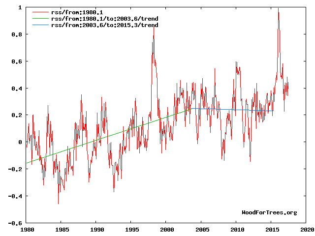
Fig 4. RSS trends showing the millennial cycle temperature peak at about 2003 (14)
Figure 4 illustrates the working hypothesis that for this RSS time series the peak of the Millennial cycle, a very important “golden spike”, can be designated at 2003/4
The RSS cooling trend in Fig. 4 was truncated at 2015.3 , because it makes no sense to start or end the analysis of a time series in the middle of major ENSO events which create ephemeral deviations from the longer term trends. By the end of August 2016, the strong El Nino temperature anomaly had declined rapidly. The cooling trend is likely to be fully restored by the end of 2019.
6..This “golden spike”correlates with the solar activity peak (neutron low) at about 1991 in Fig 10 above. There is a 12 year +/- delay between the solar driver peak and the temperature peak because of the thermal inertia of the oceans.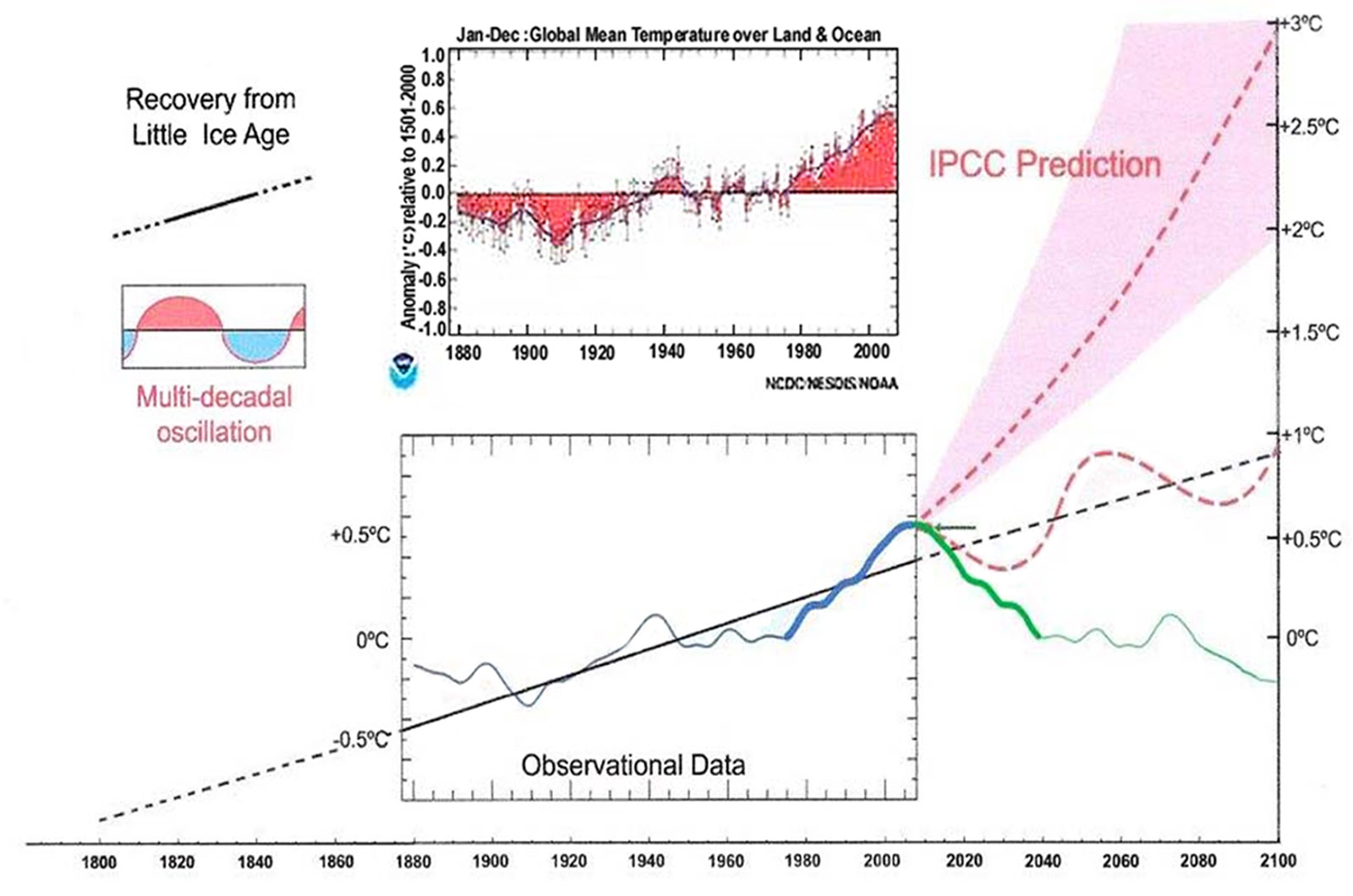
7 Forecasts to 2100 are given below
Fig. 12. Comparative Temperature Forecasts to 2100.
Fig. 12 compares the IPCC forecast with the Akasofu (31) forecast (red harmonic) and with the simple and most reasonable working hypothesis of this paper (green line) that the “Golden Spike” temperature peak at about 2003 is the most recent peak in the millennial cycle. Akasofu forecasts a further temperature increase to 2100 to be 0.5°C ± 0.2C, rather than 4.0 C +/- 2.0C predicted by the IPCC. but this interpretation ignores the Millennial inflexion point at 2004. Fig. 12 shows that the well documented 60-year temperature cycle coincidentally also peaks at about 2003.Looking at the shorter 60+/- year wavelength modulation of the millennial trend, the most straightforward hypothesis is that the cooling trends from 2003 forward will simply be a mirror image of the recent rising trends. This is illustrated by the green curve in Fig. 12, which shows cooling until 2038, slight warming to 2073 and then cooling to the end of the century, by which time almost all of the 20th century warming will have been reversed.
The establishment climate scientists made a schoolboy error of scientific judgement by projecting trends straight ahead across the millennial peak turning point. The whole UNFCC circus which has led to the misuse of trillions of dollars is based on the ensuing delusionary projections of warming.
The latest Unscientific American has a piece from Kate Marvel from the Columbia University Anthropogenic Warming support group discussing clouds. Fig 11 from the paper linked above gives a neat example of the warming peak and inflection point seen in the cloud cover and global temperature.
I have been for many years, why there is no cloudess data after 2010. Has anybody any information, why we do not have this data?
Not sure what that means or how the figure was arrived at. I don’t think we are told, are we?
I only have access to the surface model data via KNMI: https://climexp.knmi.nl/start.cgi
There are dozens of CMIP5 surface models (or variants) for each ‘pathway’, or CO2 emission scenario. The KNMI site allows you to download the ‘mean’ for each scenario, to save on the leg work. As far as the surface data are concerned, it’s fair to say that, while the models are generally running warmer than the observations, the difference isn’t huge.
It depends how you smooth things out, but if you just compare monthly or annual values, then there have been months/years recently when observations have been running warmer than the mean of the model outputs; even in the highest CO2 emissions scenario – 8.5.
If yo smooth it out by a few years, capturing the slightly cooler period around 2012, then the models are running a bit warmer than the observations; but not by much.
The description of the calculation is somewhere in former replies.
I think that I saw a comment that it is not a proper procedure to compare the Climate Sensitivity (CS) results of the IPCC’s simple model (as I call it) and the results of GCMs. I think that according to this comment, CS should be used for diagnosis only. For what diagnosis??
It is not so. The artificial specification of CS (doubling the CO2 concentration from 280 to 560 ppm) has been created just for easy comparisons of different climate models. It makes also a lot of sense, because this concentration change is so great that the differences between the models come clearly out.
I have shown that the IPCC’s simple model gives (1.85 degrees) practically the same CS value as the official figure of IPCC, which is 1.9 C ± 0.15 C, and which is based on GCMs. If the results of two models give the same CS, then the science behind the calculations is the same. Simple like that.
It seems to be a great surprise that the IPCC’s simple model works like this and the warming calculations of IPCC for RCP scenarios are also based on this model as well as the baseline scenario calculations of the Paris Climate Agreement.
Some words about the simple model of IPCC, which is
dT = CSP*RF, (1)
RF = k * ln(C/280) (2)
where CSP is Climate Sensitivity Parameter, and C is CO2 concentration (ppm). IPCC’s choices have been CSP = 0.5 K/(W/m2) and k = 5.35 and my choices are CSP = 0.27 and k = 3.12.
So, I think that the form of the model is correct. It is question about very small changes in the outgoing LW radiation. For example, the CO2 increase form 280 ppm to 560 ppm decreases the outgoing LW radiation by 2.29 W/m2 in clear sky conditions. This decrease is compensated by the elevated surface temperature of 0.69 degrees.
This change can be compared to the total radiation, which is about 260 W/2. The change is about 0.9 % only. I am familiar with the creation of process dynamic models. They are all based on the linearization around the operating point. This situation is very similar. The changes are so small that the simple linear models are applicable. The complicated GCMs are needed to calculate three dimensional changes but the global result is the same as by the simple model.
“CSP is Climate Sensitivity Parameter”
CSP is the equilibrium CSP. It tells what the notional increase in T would be, after abrupt change RF, when everything has settled down, which would take centruies. That is why more elaborate definitions of transient sensitivity are devised. But they have conditions.
Here is what Sec 6.1.1 of the TAR says about it, including the tangential reference to old-time use of 0.5 (my bold)
The CSP value of 0.5 is used for calculating the TCS values, which means that the only positive feedback is water feedback: TCS =0.5*3.7 = 1.85 degrees. The ECS according to AR5 is between 1.5 to 4.5 C which means an average value of 3.0 C. In Table 9.5 of AR5 has been tabulated the key figures of 30 GCMs and the average value of these 30 GCMs is 3.2 C. When using the simple model of IPCC, the corresponding CSP-values are 0.81 and 0.87. In this Table 9.5 is also tabulated the average CSP values of 30 GCMs for ECS and it is 1.0.
Roughly we can say that the ECS can be calculated by multiplying TCS by 2. The ECS values are highly theoretical, because IPCC itself does not use it for calculating real-world values: RCP warming values during this century are calculated using the CSP value of 0.5.
“The CSP value of 0.5 is used for calculating the TCS values”
This is all hopeless if you don’t have a source for the 0.5 number. If it’s the number referred to in TAR 6.1.1, it is explicitly ECS. You can’t just say we’ll call it TCS and use the ECS number. There are different definitions of TCS, none applicable here.
First off, as the author admits, this is an exercise in curve fitting. He has four different curve fits, which if I’ve counted correctly have no less than nine! tunable parameters. With that many parameters, it would be surprising if he could NOT fit the data. I refer the reader to Freeman Dyson’s comments on tunable parameters for the reasons why multi-parameter fits are such a bad idea..
Next, the author seems unaware that one way to test such parameterized fits is to divide the data in half, and run the fitting procedure on just the first half separately. Then, using those parameters, see how well that emulates the second half of the data.
Then repeat that in reverse order, running the fit on the second half and using that to backcast the first half.
Since the author hasn’t reported the results of such a test, I fear that his results have no meaning. Seriously, folks, if you can’t fit that curve with four equations using nine tunable parameters, you need to turn in your credentials on the way out … what he has done is a trivial exercise.
w.
I expected that this kind of comments will emerge. I just remind that the RF equation of Myhre et al. is a result of curve fitting and the result is a logarithmic relationship between the CO2 concentration and the RF value. In this equation there is only one parameter (5.35). I have done the same thing and my value for the parameter is 3.12. So,I know what I am talking about.
Hansen et al. have also developed an equation for the same purpose and they selected a polynomial expression having together 5 parameters. According to Willis, the model of Hansen et al. is just lousy science because of the number of parameters. The truth is that the number of parameters have nothing to do, which model is the best. It is just a question of curve fitting. Of course, a simple model is nice, and it is easy to use. The decisive thing in the end is this: Are the scientific calculations correct in calculating each pair of data points for curve fitting. The number of parameters have no role in this sense.
Yes, I have used curve fitting in all four cases: The Sun effect is pure empirical equation (and so is the equation of gravity, by the way). I could have used the theoretical values of Scafetta for AHR but I preferred the empirical value (one parameter), volcano effects are empirical, and the eggects of GH gases are theoretical in the same way as in the case of IPCC.
aveollila November 22, 2017 at 12:32 pm Edit
There is a solid physical basis for the claim that the relationship between concentration and forcing is logarithmic. Your work has absolutely no such basis.
James Hansen??? You are putting up James Hansen’s work as an ideal?
Get serious. Hansen is a wild alarmist whose work is a scientific joke.
I begin to despair. What you have done is a curve fitting exercise with a large number of parameters. You seem surprised that you’ve gotten a good fit, but with nine parameter that is no surprise at all. It would only be surprising if you couldn’t fit the data, given the head start.
I detailed above how you should have tested the results.
The fact that you either have not done the tests or have not reported them clearly indicates that you are out of your depth. Come back when you have done the tests and report the results, and we’ll take it from there.
w.
Willis Eschenbach commented – “James Hansen??? You are putting up James Hansen’s work as an ideal?
Get serious. Hansen is a wild alarmist whose work is a scientific joke.”
hansen is and will al-
ways be a legend in climate science.
his work was groundbreaking and advanced
the field more
than anyone since manabe, and his
public warnings even
more than that.
when the history of 20th
Cen climate science is fully written,
JHansen will easily
be a top 10 player.
Crackers,
Please state the “groundbreaking” contributions which you imagine Hansen to have made to “climate science”. Thanks.
https://en.wikipedia.org/wiki/James_Hansen#Research_and_publications
https://en.wikipedia.org/wiki/James_Hansen#Analysis_of_climate_change_causation
https://en.wikipedia.org/wiki/James_Hansen#Climate_change_activism
Hansen led the effort to
calculate a rigorous GMST.
His 1988 congressional
testimony changed the
landscape of AGW. (“global
warming has begun)
his 1981
paper in Science was
and will always be
a masterpiece.
I have been criticized that the so-called IPCC’s simple climate model cannot be used for calculating the temperature value for the year 2016. If this model cannot be used, what model can be used and what is the temperature change value for 2016? If a climate model cannot be used for calculating the warming value for a certain year, is it a model at all? It looks like that there is a mysterious climate model, which can be used for calculating temperature increase after 100 years, but nobody knows what is that model and what is more: you should not call it “a IPCC’s climate model”.
I just remind you once more: The warming impacts of RCPs and the Paris climate agreement are based on the IPCC’s science. I have shown in detail, what is this science. Those who criticize my evidences, have not shown any signs about the alternative ways of calculations.
the ipcc doesn’t make
models, they assess
them. and they do that for
many more than one. there is
no “ipcc climate model.”
I don’t see what Scafetta’s 59.6yr Saturn-Jupiter tri-synodic period has to do with an observed AMO envelope of 65-69yrs?
It has nothing to do with it … but that’s never stopped them before and won’t stop them now.
w.
How does one link incomplete and grossly adjusted data to a model that does not represent the climate system?
Climate models have a lot of warming tuned in from hindcast.
“Climate models have a lot of warming tuned in from hindcast.”
how so, exactly?
A science teacher of mine one explained entropy: “If you add a drop of wine to a gallon of sewage you get sewage. If you add a drop of sewage to a gallon of wine you get sewage.”
The models don’t work. You cannot ‘rescue’ them by blending them with data.