Propagation of Error and the Reliability of Global Air Temperature Projections
Guest essay by Pat Frank
Regular readers at Anthony’s Watts Up With That will know that for several years, since July 2013 in fact, I have been trying to publish an analysis of climate model error.
The analysis propagates a lower limit calibration error of climate models through their air temperature projections. Anyone reading here can predict the result. Climate models are utterly unreliable. For a more extended discussion see my prior WUWT post on this topic (thank-you Anthony).
The bottom line is that when it comes to a CO2 effect on global climate, no one knows what they’re talking about.
Before continuing, I would like to extend a profoundly grateful thank-you! to Anthony for providing an uncensored voice to climate skeptics, over against those who would see them silenced. By “climate skeptics” I mean science-minded people who have assessed the case for anthropogenic global warming and have retained their critical integrity.
In any case, I recently received my sixth rejection; this time from Earth and Space Science, an AGU journal. The rejection followed the usual two rounds of uniformly negative but scientifically meritless reviews (more on that later).
After six tries over more than four years, I now despair of ever publishing the article in a climate journal. The stakes are just too great. It’s not the trillions of dollars that would be lost to sustainability troughers.
Nope. It’s that if the analysis were published, the career of every single climate modeler would go down the tubes, starting with James Hansen. Their competence comes into question. Grants disappear. Universities lose enormous income.
Given all that conflict of interest, what consensus climate scientist could possibly provide a dispassionate review? They will feel justifiably threatened. Why wouldn’t they look for some reason, any reason, to reject the paper?
Somehow climate science journal editors have seemed blind to this obvious conflict of interest as they chose their reviewers.
With the near hopelessness of publication, I have decided to make the manuscript widely available as samizdat literature.
The manuscript with its Supporting Information document is available without restriction here (13.4 MB pdf).
Please go ahead and download it, examine it, comment on it, and send it on to whomever you like. For myself, I have no doubt the analysis is correct.
Here’s the analytical core of it all:
Climate model air temperature projections are just linear extrapolations of greenhouse gas forcing. Therefore, they are subject to linear propagation of error.
Complicated, isn’t it. I have yet to encounter a consensus climate scientist able to grasp that concept.
Willis Eschenbach demonstrated that climate models are just linearity machines back in 2011, by the way, as did I in my 2008 Skeptic paper and at CA in 2006.
The manuscript shows that this linear equation …
![]()
… will emulate the air temperature projection of any climate model; fCO2 reflects climate sensitivity and “a” is an offset. Both coefficients vary with the model. The parenthetical term is just the fractional change in forcing. The air temperature projections of even the most advanced climate models are hardly more than y = mx+b.
The manuscript demonstrates dozens of successful emulations, such as these:

Legend: points are CMIP5 RCP4.5 and RCP8.5 projections. Panel ‘a’ is the GISS GCM Model-E2-H-p1. Panel ‘b’ is the Beijing Climate Center Climate System GCM Model 1-1 (BCC-CSM1-1). The PWM lines are emulations from the linear equation.
CMIP5 models display an inherent calibration error of ±4 Wm-2 in their simulations of long wave cloud forcing (LWCF). This is a systematic error that arises from incorrect physical theory. It propagates into every single iterative step of a climate simulation. A full discussion can be found in the manuscript.
The next figure shows what happens when this error is propagated through CMIP5 air temperature projections (starting at 2005).

Legend: Panel ‘a’ points are the CMIP5 multi-model mean anomaly projections of the 5AR RCP4.5 and RCP8.5 scenarios. The PWM lines are the linear emulations. In panel ‘b’, the colored lines are the same two RCP projections. The uncertainty envelopes are from propagated model LWCF calibration error.
For RCP4.5, the emulation departs from the mean near projection year 2050 because the GHG forcing has become constant.
As a monument to the extraordinary incompetence that reigns in the field of consensus climate science, I have made the 29 reviews and my responses for all six submissions available here for public examination (44.6 MB zip file, checked with Norton Antivirus).
When I say incompetence, here’s what I mean and here’s what you’ll find.
Consensus climate scientists:
1. Think that precision is accuracy
2. Think that a root-mean-square error is an energetic perturbation on the model
3. Think that climate models can be used to validate climate models
4. Do not understand calibration at all
5. Do not know that calibration error propagates into subsequent calculations
6. Do not know the difference between statistical uncertainty and physical error
7. Think that “±” uncertainty means positive error offset
8. Think that fortuitously cancelling errors remove physical uncertainty
9. Think that projection anomalies are physically accurate (never demonstrated)
10. Think that projection variance about a mean is identical to propagated error
11. Think that a “±K” uncertainty is a physically real temperature
12. Think that a “±K” uncertainty bar means the climate model itself is oscillating violently between ice-house and hot-house climate states
Item 12 is especially indicative of the general incompetence of consensus climate scientists.
Not one of the PhDs making that supposition noticed that a “±” uncertainty bar passes through, and cuts vertically across, every single simulated temperature point. Not one of them figured out that their “±” vertical oscillations meant that the model must occupy the ice-house and hot-house climate states simultaneously!
If you download them, you will find these mistakes repeated and ramified throughout the reviews.
Nevertheless, my manuscript editors apparently accepted these obvious mistakes as valid criticisms. Several have the training to know the manuscript analysis is correct.
For that reason, I have decided their editorial acuity merits them our applause.
Here they are:
- Steven Ghan___________Journal of Geophysical Research-Atmospheres
- Radan Huth____________International Journal of Climatology
- Timothy Li____________Earth Science Reviews
- Timothy DelSole_______Journal of Climate
- Jorge E. Gonzalez-cruz__Advances in Meteorology
- Jonathan Jiang_________Earth and Space Science
Please don’t contact or bother any of these gentlemen. On the other hand, one can hope some publicity leads them to blush in shame.
After submitting my responses showing the reviews were scientifically meritless, I asked several of these editors to have the courage of a scientist, and publish over meritless objections. After all, in science analytical demonstrations are bullet proof against criticism. However none of them rose to the challenge.
If any journal editor or publisher out there wants to step up to the scientific plate after examining my manuscript, I’d be very grateful.
The above journals agreed to send the manuscript out for review. Determined readers might enjoy the few peculiar stories of non-review rejections in the appendix at the bottom.
Really weird: several reviewers inadvertently validated the manuscript while rejecting it.
For example, the third reviewer in JGR round 2 (JGR-A R2#3) wrote that,
“[emulation] is only successful in situations where the forcing is basically linear …” and “[emulations] only work with scenarios that have roughly linearly increasing forcings. Any stabilization or addition of large transients (such as volcanoes) will cause the mismatch between this emulator and the underlying GCM to be obvious.”
The manuscript directly demonstrated that every single climate model projection was linear in forcing. The reviewer’s admission of linearity is tantamount to a validation.
But the reviewer also set a criterion by which the analysis could be verified — emulate a projection with non-linear forcings. He apparently didn’t check his claim before making it (big oh, oh!) even though he had the emulation equation.
My response included this figure:

Legend: The points are Jim Hansen’s 1988 scenario A, B, and C. All three scenarios include volcanic forcings. The lines are the linear emulations.
The volcanic forcings are non-linear, but climate models extrapolate them linearly. The linear equation will successfully emulate linear extrapolations of non-linear forcings. Simple. The emulations of Jim Hansen’s GISS Model II simulations are as good as those of any climate model.
The editor was clearly unimpressed with the demonstration, and that the reviewer inadvertently validated the manuscript analysis.
The same incongruity of inadvertent validations occurred in five of the six submissions: AM R1#1 and R2#1; IJC R1#1 and R2#1; JoC, #2; ESS R1#6 and R2#2 and R2#5.
In his review, JGR R2 reviewer 3 immediately referenced information found only in the debate I had (and won) with Gavin Schmidt at Realclimate. He also used very Gavin-like language. So, I strongly suspect this JGR reviewer was indeed Gavin Schmidt. That’s just my opinion, though. I can’t be completely sure because the review was anonymous.
So, let’s call him Gavinoid Schmidt-like. Three of the editors recruited this reviewer. One expects they called in the big gun to dispose of the upstart.
The Gavinoid responded with three mostly identical reviews. They were among the most incompetent of the 29. Every one of the three included mistake #12.
Here’s Gavinoid’s deep thinking:
“For instance, even after forcings have stabilized, this analysis would predict that the models will swing ever more wildly between snowball and runaway greenhouse states.”
And there it is. Gavinoid thinks the increasingly large “±K” projection uncertainty bars mean the climate model itself is oscillating increasingly wildly between ice-house and hot-house climate states. He thinks a statistic is a physically real temperature.
A naïve freshman mistake, and the Gavinoid is undoubtedly a PhD-level climate modeler.
The majority of Gavinoid’s analytical mistakes include list items 2, 5, 6, 10, and 11. If you download the paper and Supporting Information, section 10.3 of the SI includes a discussion of the total hash Gavinoid made of a Stefan-Boltzmann analysis.
And if you’d like to see an extraordinarily bad review, check out ESS round 2 review #2. It apparently passed editorial muster.
I can’t finish without mentioning Dr. Patrick Brown’s video criticizing the youtube presentation of the manuscript analysis. This was my 2016 talk for the Doctors for Disaster Preparedness. Dr. Brown’s presentation was also cross-posted at “andthentheresphysics” (named with no appreciation of the irony) and on youtube.
Dr. Brown is a climate modeler and post-doctoral scholar working with Prof. Kenneth Caldiera at the Carnegie Institute, Stanford University. He kindly notified me after posting his critique. Our conversation about it is in the comments section below his video.
Dr. Brown’s objections were classic climate modeler, making list mistakes 2, 4, 5, 6, 7, and 11.
He also made the nearly unique mistake of confusing an root-sum-square average of calibration error statistics with an average of physical magnitudes; nearly unique because one of the ESS reviewers made the same mistake.
Mr. andthentheresphysics weighed in with his own mistaken views, both at Patrick Brown’s site and at his own. His blog commentators expressed fatuous insubstantialities and his moderator was tediously censorious.
That’s about it. Readers moved to mount analytical criticisms are urged to first consult the list and then the reviews. You’re likely to find your objections critically addressed there.
I made the reviews easy to apprise by starting them with a summary list of reviewer mistakes. That didn’t seem to help the editors, though.
Thanks for indulging me by reading this.
I felt a true need to go public, rather than submitting in silence to what I see as reflexive intellectual rejectionism and indeed a noxious betrayal of science by the very people charged with its protection.
Appendix of Also-Ran Journals with Editorial ABM* Responses
Risk Analysis. L. Anthony (Tony) Cox, chief editor; James Lambert, manuscript editor.
This was my first submission. I expected a positive result because they had no dog in the climate fight, their website boasts competence in mathematical modeling, and they had published papers on error analysis of numerical models. What could go wrong?
Reason for declining review: “the approach is quite narrow and there is little promise of interest and lessons that transfer across the several disciplines that are the audience of the RA journal.”
Chief editor Tony Cox agreed with that judgment.
A risk analysis audience not interested to discover there’s no knowable risk to CO2 emissions.
Right.
Asia-Pacific Journal of Atmospheric Sciences. Songyou Hong, chief editor; Sukyoung Lee, manuscript editor. Dr. Lee is a professor of atmospheric meteorology at Penn State, a colleague of Michael Mann, and altogether a wonderful prospect for unbiased judgment.
Reason for declining review: “model-simulated atmospheric states are far from being in a radiative convective equilibrium as in Manabe and Wetherald (1967), which your analysis is based upon.” and because the climate is complex and nonlinear.
Chief editor Songyou Hong supported that judgment.
The manuscript is about error analysis, not about climate. It uses data from Manabe and Wetherald but is very obviously not based upon it.
Dr. Lee’s rejection follows either a shallow analysis or a convenient pretext.
I hope she was rewarded with Mike’s appreciation, anyway.
Science Bulletin. Xiaoya Chen, chief editor, unsigned email communication from “zhixin.”
Reason for declining review: “We have given [the manuscript] serious attention and read it carefully. The criteria for Science Bulletin to evaluate manuscripts are the novelty and significance of the research, and whether it is interesting for a broad scientific audience. Unfortunately, your manuscript does not reach a priority sufficient for a full review in our journal. We regret to inform you that we will not consider it further for publication.”
An analysis that invalidates every single climate model study for the past 30 years, demonstrates that a global climate impact of CO2 emissions, if any, is presently unknowable, and that indisputably proves the scientific vacuity of the IPCC, does not reach a priority sufficient for a full review in Science Bulletin.
Right.
Science Bulletin then courageously went on to immediately block my email account.
*ABM = anyone but me; a syndrome widely apparent among journal editors.
Pat,
This has already been explained to you numerous, so it’s unlikely that this attempt will be any more successful than previous attempts. The error that you’re trying to propagate is not an error at every timestep, but an offset. It simply influences the background/equilibrium state, rather than suggesting that there is an increasing range of possible states at every step. For example, if we ran two simulations with different solar forcings (but everything else the same), this wouldn’t suddenly mean that they would/could diverge with time, it would mean that they would settle to different background/equilibrium states.
@ur momisugly and Then There’s Physics
I’m a layman and no mathematician but having read the first few pages of the paper it seems to me that your points are answering the wrong question. (?)
The point made, or so it appears to me, is that where there is uncertainty in the assumptions being made within a model then – if, as they should be those uncertainties are expressed and included within the model, as the time-steps are calculated then the uncertainty grows into a wide band with a diverging top and bottom spread of values. In other words they diverge.
If the uncertainties are not included as part of the model then surely it is linear and unable to produce meaningful results?
If you have multiple uncertainties, as in climate, which are input into a model then the spread or divergence must become even greater with time.
Some of those would seem to be (but far from limited too) temperatures and effect on on atmospheric water vapour levels; cloud formation and cloud cover; solar activity; volcanic activity etc etc. each would have an effect on some of the others and with a amount of uncertainty which would need to be expressed.
As I said, I am a layman and would appreciate it if you could enlighten me.
Thanks
The point made, or so it appears to me, is that where there is uncertainty in the assumptions being made within a model then – if, as they should be those uncertainties are expressed and included within the model, as the time-steps are calculated then the uncertainty grows into a wide band with a diverging top and bottom spread of values. In other words they diverge.
Except this is not correct. An uncertainty only propagates if it applies at every step (i.e., if there is some uncertainty in the expected value at every step). If, however, some value is “wrong” by some amount that is the same at all time steps, then this does not propagate (by “wrong” I mean potentially different to reality). In this case, it is quite possible that the cloud forcing is “wrong” by a few W/m^2. What this would mean is that the equilibrium state would also then be “wrong”. It doesn’t mean, however, that the range of possible equilibrium states will grow with time, since this error does not propagate.
As I mentioned in the first comment, imagine we could run a perfect model in which every parameter exactly matched reality. Now imagine running the same model, apart from the Solar forcing being different by a few W/m^2. What would happen is that this would change the equilibrium state (there would be a constant offset between the “perfect” model and this other model). It would not mean that the difference between the model with the different solar forcing, and the “perfect” model would grow with time.
“An uncertainty only propagates if it applies at every step”
Um… No. A climate model is essentially an attempt to integrate a bunch of co-dependent variables numerically. If you knew anything about numerical integration, you would know that errors propagate wildly. The tool is, fundamentally, unsuited to the purpose it is being put.
ATTP, Stop focusing on the output result and thinking it’s error within an acceptable range therefore ok to propagate.
The issue is that the uncertainty that is propagated at each time step isn’t seen in the output because the output has been constrained by design to be within “reasonable” values. This is seen to be evidence the model is “doing the right thing” but the real problem is that at every single time step the output is meaningless for a climate calculation because the climate signal is much smaller than the error and what we’re left with is a fitted result.
Now you’ll arc up and suggest CGMs aren’t fits and are based on physics but again you’re mistaken because there are components (eg clouds) that aren’t and they’re approximations, they’re fits and by including them the models themselves are reduced to fits.
The whole GCM enterprise further relies on the assumption that errors cancel at each step throughout and that’s a ridiculous assumption. Completely unjustified and most certainly incorrect. In fact there is a small (unintentionally) built in bias that results in an expected result.
“imagine we could run a perfect model in which every parameter exactly matched reality.”
Yet you are UNABLE to run one where ANY parameter matches reality.
The ONLY thing you have is hallucinogenic anti-science IMAGINATION and FAIRY-TAILS
” If you knew anything about numerical integration, you would know that errors propagate wildly.”
I know lots about numerical integration (so does ATTP). I have spent a large part of my professional life doing it, in computational fluid dynamics, a regular engineering activity of which GCMs are a subset. Your statement is nonsense.
There’s no reason that difference would be equal over time. That’s a sign you have created a linear model, and it’s a decidedly non-linear system you’re modeling.
If this is what you think you guys are lost.
Micro,
I totally agree. This is probably the most telling comment of this whole discussion.
rip
ATTP, I was thinking about this more, you totally do not get that WV acts as a regulating medium, it actively alters the out going radiation response based on cooling temperatures, and not the stupid SB 4th pwr decay, this is on top of that, it’s the bends in the clear sky cooling profile. And since this is decidedly non-linear, and it controls the response to Co2, you’re not accounting for it in your models.
Think about how much the atm column shrinks at night. when it’s calm, it can only cool by radiation, and radiation is omni directional. Also for every gram of water vapor, there is a 4.21 J exchange of IR for a condense – reevaporation cycle as let’s say a 3,000 meter tall stack cools.


Interestingly it cools really quickly till air temps near dew point, then it stops cooling. It’s just there’s about -50W/m^2 of radiation to space just through the optical window based on SB calculations, yet net radiation is less than -20W/m^2. There’s about 35W’m^2 of sensible heat keeping the surface temp from falling as quickly.
There’s a 90F differences in the middle of the spectrum, I’ve measured over 100F differences.
How much energy is about 1 psi change between morning min T and afternoon Max temps at the surface(plus enthalpy lost, water condensed)? Oh wait, without the pressure change, average of about 3,300W/m^3.
attp says:
Funny, your example uses the ONLY independent variable in the whole shabang. Use any other co-dependent variable, and your example is busted.
Only in linear systems
In chaotic systems a single butterfly flapping its wings once….
…and that is a huge point. Climate models treat the climate as a linear system, because we do not have computational tools that can address the uncertainty of non linear systems.
To accept chaotic behaviour is merely to affirm ‘we can’t predict where this is going at all’. Or to put it in the vernacular. Climate science is at that level just bunk.
Even those people here who look for ‘cycles’ in climate with the ardent passion of ‘chemtrail’ observers, may in the end be barking up only a slightly less egregious gum tree than the climate scientists. Chaotic behaviour produces quasi-periodic fluctuations: That is over short times spans it may look briefly like a cycle, but then as it moves towards new attractors, it will enter a different ‘cycle’ and those of us who have built electronic circuits utilising chaotic feedback (super regenerative radios) know that, absent of a forcing signal, what you get is NOISE pure and simple, with no detectable single spectral component.
Nothing is more infuriating than to have someone lecturing you on the characteristics of linear equations challenging you to disprove their finer points, when your whole position is predicated in a provable assertion that what is being modelled cannot be represented by linear equations in the first place.
“Except this is not correct. An uncertainty only propagates if it applies at every step (i.e., if there is some uncertainty in the expected value at every step). If, however, some value is “wrong” by some amount that is the same at all time steps”
incorrect, the value increases with each step over time, you are a completely anti scientific chappy, clueless
Typical attp tactic, start off with a lie then spin sophistry round your false strawman.
Micro thanks for exposing ATTP’s cut and paste knowledge. Once you get in depth with him, he vanishes every time and runs back to his echo chamber
this annual average ±4.0 Wm-2 year-1 uncertainty in simulated LWCF is approximately ±150% larger than all the forcing due to all the anthropogenic greenhouse gases put into the atmosphere since 1900 (~2.6 Wm-2), and approximately ±114× larger than the average annual ~0.035 Wm-2 year-1 increase in greenhouse gas forcing since 1979
The error DOES in my opinion propagate.
And Then There’s Physics says If, however, some value is “wrong” by some amount that is the same at all time steps, then this does not propagate.
If the correction for cloud fraction error was a simple linear adjustment to models to correct the error, we would never have known about it. The adjustment would have been applied, and the model prediction would have aligned with observed cloud fraction.
Since nobody can accurately predict how clouds respond to GHG forcing, the margin for error grows with every iteration step, The uncertainty of how clouds will respond to the GHG forcing applied in a single step has to be carried through to the next iteration.
When the margin for error drastically exceeds what is physically plausible, I think we can safely assume the predictions of the model are total nonsense.
Page 23 of Pat Frank’s paper, hindcast cloud fraction error of global climate models.
ATTP says,
This assumes a linear response. It assumes that climate (and thus, presumably, weather) is a linear function of forcings.
If the initial value is “wrong” by some amount – or inaccurate by some amount – then that will affect the next iteration in some way.
If the next iteration is affected by the same amount every single time then the response is always constant.
Once again we have pseudoscience pretending that clouds don’t exist. That phase changes (water vapour to water droplets, for example) are smooth.
Why does ATTP worry about a declining Arctic Icecap when he doesn’t believe in non-linear phase changes? Melting can’t exist in his understanding of climate!
Except he has no understanding. He’s just a climate fanatic. It’s faith, not science.
You’ve got the essence, Old England, “that where there is uncertainty in the assumptions being made within a model then – if, as they should be those uncertainties are expressed and included within the model, as the time-steps are calculated then the uncertainty grows into a wide band…
You have grasped the central point that continually eludes ATTP and virtually every single climate modeler.
The error is systematic, resident in the model, and is introduced into a simulation by the model itself. It enters every simulation time-step, and necessarily produces an increasing uncertainty in the projection.
Look at ATTP’s reply to you.. His “wrong by some amount” supposes a constant offset error and is a completely wrong description of the systematic error.
Look at manuscript Figure 5. Every single model makes has a different error profile with positive and negative excursions. I pointed this out to ATTP in prior conversations. He ignores it. Perhaps because he doesn’t understand the significance. Change the parameter set of any one model, and its error profile will be different.
But ATTP (and others) want to add up all the errors to get one number, and then assume that number is a constant offset error that will correct any model expectation value to be error-free. His (their) idea is beyond parody.
Then he goes on to suppose statistical uncertainty is physical error, i.e., ATTP: “the range of possible equilibrium states will grow with time, since this error does not propagate,”
ATTP makes a standard mistake of my reviewers, here specifically number 6, but he has already also made mistakes 4, 5, 7 and 8.
He makes those same mistakes over, and over again.
TimTheToolMan gets it right, as usual.
Tim, do you have any idea why uncertainty is so opaque to climate modelers?
It’s dead obvious to any experimental scientist or engineer.
In this post, Nick Stokes admitted that GCMs are engineering models. I.e., Nick: “a regular engineering activity of which GCMs are a subset.”
Engineering models are useless outside their calibration bounds. Nick has repudiated the entire global warming scary-2100 enterprise.
Yet another inadvertent validation in an attempted refutation. Thank-you, Nick.
Eric Worrall, your comment is right on.
Thanks for posting Figure 5. It shows that every model has a different error profile, with positive and negative excursions.
Mere inspection of the figure shows how ludicrous is ATTP’s idea that all those errors should be merely added together into a number. And then subtracted away to make everything accurate. Only in consensus climate science.
“Engineering models are useless outside their calibration bounds.”
So what are the “calibration bounds” of, say, Nastran? Or Fluent, or Ansys? Pat, you don’t have a clue about engineering models.
well it’s obvious you don’t understand this.
Calibration isn’t defined by the simulator, but the models as applied to the design you’re evaluating. And it’s in comparison to the real circuit in operation.
Pat writes
I dont think it is. I think even Nick gets it and one day might even accept it (no Nick, it doesn’t mean your CFD work is dead, or weather models are wrong – models have their place still!) but no climate modeler can admit to it because it’d be well…a career limiting move. And as the GCMs are the cornerstone to so much of our science today, untangling the mess would be horrendous. Better to let sleeping dogs lie.
Pat Frank,
Look at manuscript Figure 5.
Ok, it shows latitudinal profiles of 25-year averaged model cloud fraction error versus cloud fraction observations averaged over a similar timescale. It demonstrates latitudinal error offsets between models and observations, as well as showing differences between models.
Every single model makes has a different error profile with positive and negative excursions.
Yes, this is well known and clearly understood by ATTP. Different models, different offsets.
Change the parameter set of any one model, and its error profile will be different.
Yes, this would obviously be true but how is it relevant to error propagation within a projection? Within an individual model projection run the parameter set will remain the same, thereby maintaining the same offset error.
Put in context of your Figure 5, your error propagation suggests that those error profiles should change quite dramatically over time. Why would that happen?
Nick Stokes, no matter your diversionary sneering, I’m clued in enough to know that engineering models are unreliable outside their calibration bounds.
Paulski0 “Within an individual model projection run the parameter set will remain the same, thereby maintaining the same offset error.”
Not correct, for two reasons. The parameters are not unique. They have large uncertainty widths. One can get the same apparent error with different suites of parameters. A given error is just representative. It does not transmit the true range of model errors. The uncertainty is made cryptic unless this is taken into account.
Second, even with unchanging parameter sets, any given projection simulation step is wrong, but to some unknown amount. Those wrong climate states are projected forward. Every step begins with initial value errors.
The projection error from step to step therefore varies, and in unknowable ways.
In a futures projection, one can’t know the errors. One only knows the uncertainty, by way to the propagated calibration error statistic. And uncertainty grows with each projection step because of increasing ignorance of the relative positions of the simulated state and the correct physical state in phase space.
Error propagation says nothing about error profiles in projection simulations. It addresses the reliability of the projection. Not its error.
I think you and the reviewers may be missing the point here attp. Millions spent on building climate models…and a simple linear model can recreate them very closely…..surely this is worth publishing and worth investigating further?
A simple linear model is what climate models are, stripped of decorative complexity, but whilst models may be represented by a model of that nature, reality it seems is just too complicated for that class of model to have a snowballs chance in hell of representing the vagaries of actual climate.
So I dont know what you are saying, but its not worth spending a copper nickel on.
I looked into cutting edge attempts by seriously bright mathematicians to even discern whether a given set of non linear partial derivatives led to a bounded set of solutions (broadly, a climate that never goes below snowball earth or boils the oceans dry) and we cant even do THAT. Observationally climate is amazingly stable.
But wobbles a lot as well.
And we have absolutely no idea whether it could one day wobble off to a whole new regime, just because a butterfly flapped its wings, let alone by injecting tons of CO2 into it. All we can say is that in times gone by, when CO2 was way greater than it is today, or is likely to be in the foreseeable future, the climate seems to have been stable enough for life to flourish.
The state of climate change science stripped down to the actual science, which is almost none, is simply stated
1/. We don’t know.
2/. Even if we did know the partial differentials governing it, we still wouldn’t know what the climate will do.
3/. We lack both the mathematics and the computational power to ever know better than that.
4/. Climate change is therefore not worth spending any grant money on.
5/. Even WUWT has no function beyond pointing out points 1, 2, 3 and 4.
6/. The IPCC is an organization without any purpose, since it exists to advise governments on situations that have no existence in reality.
7/. Renewable energy is therefore a crock of excrement, a pointless waste of money.
8/. Anyone who disagrees with any of the points above is like a holocaust denier.
9/. There is an urgent need to set up an international organisation to help whole swathes of the population come to terms with the facts that:
– the cheque isn’t in the post
– the tooth fairy doesn’t exist
– he/she wont love you in the morning.
– ‘man made climate change’ is as real as Tinkerbelle.
Great post, Leo Smith. Your number 1 has been the conclusion of my AGW assessment from the first. 🙂
If only you were head of the US National Academy. Or Pres. Trump’s science advisor. 🙂
Another point, that I think I’ve made to Pat before, is that if he is correct he should be able to easily demonstrate this. If you’re running computational models, one way to estimate the uncertainty is to simply run them many times with different initial conditions. If the uncertainty propagates as Pat suggests, then the range of results should reflect this. As I understand it, this has been done, and they do not.
This is clear even from the published CMIP5 simulations. Pat Frank claims that the error arising from cloud uncertainty alone should accumulate to an extent of ±16°C by 2100. And he seems to infer the cloud error from disagreement between the models. But the CMIP5 models clearly do not diverge by 16°C by 2100. Here is a plot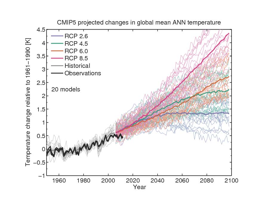
The spread is mainly due to the different scenarios; for an individual scenario it is maybe ±0.6°C.
Yes Nick
Hundreds of scam CO2-hatred “scenarios”.
NOT ONE anywhere near REALITY.
Thanks for drawing that to everybody’s attention.
Nick
And that’s your argument to establish the effectiveness of the models? Really
That’s not true Andy! Give Nick his due. ONE of those models is quite close to reality – the one at the very bottom. The rest of the models should clearly be fired. But that one should be given a prize, and it shows that temperatures in 2100 will be about the same as today. So according to the one believable model, there is no C in CAGW, and no real W either. Great! Can we all pack up and go home now? And stop wasting money on this nonsense?
@aTTP (1:24am) and Nick Stokes (2:36am)
It seems the issue is not in getting different results with different initial conditions but rather running slightly different models from the same initial condition.
The simplest setup would be to select a single tunable parameter (e.g. clouds), vary the value up or down to create 2 model formulations, and run them both from the same initial conditions. The different values may cause divergence or other feedbacks/interactions may dampen it to insignificant.
If I understand the source of Nick’s spaghetti graph, the graph demonstrates the differences between models, not the potential uncertainty inherent in any one model. Each spaghetti line has it’s own uncertainty band that it not displayed.
MJB,
Yes, you could also do what you suggest (i.e., run with the same initial conditions, but different parameters). If we consider clouds, then there is probably a range of a few W/m^2. This would correspond to potentially difference of about 1K; not even close to the +-15K suggested by Pat Frank.
As far as the spaghetti graph is concerned, I think it is a combination of individual models run more than once and different models, so you are correct that it isn’t a true uncertainty. However, it does illustrate that the range is unlikely to be as large as suggested by Pat Frank.
If constraints are being applied for each calculation then you are not getting modelled outputs but constrained outputs. Do the runs with no constraints to see the inherent validity of the underlying physics, not the hand-tailoring needed to sell a story.
But hey, if the need is to sell a story….
I find it hilarious that Nick and others still think the chart at this comment is relevant since it is pseudoscience crap:
https://wattsupwiththat.com/2017/10/23/propagation-of-error-and-the-reliability-of-global-air-temperature-projections/#comment-2643766
How can anyone think wild guesses to year 2100, be considered good science,when most of it UNVERIFIABLE! Models are a TOOL for research,not to create actual fact based science,since it lacks real data for the next 83 years. This is the what the AGW conjecture is based on,a puddle of unverifiable guesses,
Bwahahahahahahahahaha!!!
Imagine what real Meteorologists, who do short term modeling for weather prediction in the next few days know how quickly short term predictions can quickly spiral out of reality. I see them adjusting their forecasts daily,sometimes even in hours, as new information comes in,but can still be waaaaay off anyway,as they were in my city just yesterday.
Models are a TOOL for research,not a creator of data.
…and Then There’s Physics ,
You said, “However, it does illustrate that the range is unlikely to be as large as suggested by Pat Frank.” I’m not sure that you can justify that statement. The propagation of errors provides a probabilistic uncertainty range, which is an upper bound, not the most likely outcomes. That is, with numerous ensemble runs, they are most likely to cluster around the most probable values, but that doesn’t preclude them from sometimes reaching the maximum values if a large enough number of runs are made.
Extrapolating the apparent arc of the upper limit from the spaghetti plot of model runs, you reach a maximum divergence value of approximately 8.5K to 9.5K truly slightly more than half the 15K to 16K suggested
Clyde,
Normally what’s presented are 1, or 2, sigma uncertainties. This would mean that either about 66%(1 sigma), or 95% (2 sigma), of your results should lie within this range. Depending on what is presented, you would expect either 1/3 of your results (1 sigma), or 5% of your results (2 sigma), to lie outside the range. Therefore, if you ran a lot of simulations and the results never ended up outside the range, then the range would probably be too large.
Bryan,
Except, the range is mostly because of the range of emission scenarios, rather than scatter for a single scenario. Therefore, the overall range isn’t representative of some kind of model uncertainty.
sun: the RCPs aren’t “guesses,”
they’re assumptions.
Crackers,when they run to year 2100, they are indeed wild guesses,since there is ZERO evidence to support it, you are playing word game here. They are unverifiable,can’t run a hypothesis on it since most of it is far into the future,thus qualifies as wild guesses.
He writes,
“sun: the RCPs aren’t “guesses,”
they’re assumptions.”
Yawn, is this how low science literacy has fallen?
The difference between an assumption and a guess is basically the reputation of the person making them.
Fenchie77,
You are of course correct. The fact that the models require constraints is enough to invalidate them.
I doubt the is a Mechanical Engineer in the crowd that would trust his/her family’s safety to a 5th floor apartment deck that was designed with, or the design was verified by, a stress analysis (i.e., modelling) program that required constraints be placed within it to keep the calculations within reasonable ranges.
ATTP, “ one way to estimate the uncertainty is to simply run them many times with different initial conditions.”
No, it’s not. Your proposed method tells one nothing about physical uncertainty.
Mistakes 1, 3, 4, 6, and 10. Good job, ATTP.
Nick Stokes, “Pat Frank claims that the error arising from cloud uncertainty alone should accumulate to an extent of ±16°C by 2100.”
No, I don’t Nick. You’re proposing that ±16°C is a physically real temperature.
It’s an uncertainty statistic. An ignorance measure. It’s not physical error.
You’ve made mistakes 2, 6, 11 and, implicitly, 12.
You’ve many times now demonstrated knowing nothing about physical error analysis. Now it’s many times plus one more.
Pat,
Hold on. You’re suggesting the results from the models are far more uncertain than mainstream climate modellers suggest and yet you’re also suggesting that if you ran the models many times (with different initial conditions and using different parameter values) you would get an overall result that was not representative of the uncertainty. This doesn’t seem consistent.
Nick Stokes
October 23, 2017 at 2:36 am
My comment to you it is not actually about the particular point you trying to make there, but more in the aspect of contemplating the validity of the whole argument in question here about GCMs.
You see, you have a clear beautiful plot there, but really no much relevant, as it does not have the according ppm concentration trends also.
Last time I checked AGW is all about temps as per ppm…….and the correlation there…..
Ignoring this actually puts one in the position of misinterpreting the value of GCMs as an experiment…..either intentionally or not.
So when the nice plot you posted helps with your point, maybe, in its essence misleads towards a result of misinterpretation and confusion about the actual value of GCMs as an experiment, which by the way are not climate models anyhow, and very very expensive experimental tools at that.
Don’t you think that the plot you provide, the way it stands has no much support value about the RF or the fCO2 as contemplated by the AGW hypothesis one way or another?
cheers
“That’s not true Andy! Give Nick his due. ONE of those models is quite close to reality – the one at the very bottom.”
yeah, predict 1 2 3 4 5 6 and throw a dice, and one will be right.
Logic is not you nick or ATP
Idiots pretending to be scientists. Why not get English lit Mosher in on the act too
or some more of pseudo science sensitivity studies that are nothing but tuned junk driven by observations
ATTP
“Pat,
Hold on. You’re suggesting the results from the models are far more uncertain than mainstream climate modellers suggest and yet you’re also suggesting that if you ran the models many times (with different initial conditions and using different parameter values) you would get an overall result that was not representative of the uncertainty. This doesn’t seem consistent.”
It’s not inconsistent.
The models are far more uncertain than claimed, because of 1 much comes from hindcast tuning, not physics (not incomplete and some much not understood physics) Unless you are going to be uber absurd and claim that is not true
The range outcomes is uncertainy (in model physics which leas to instability (not variability)), error, and different tunings.
as with Mosher, logical examination is not for you, as usual, add Nick in there
However if you replace the linear models by non linear ones, the behaviour is exactly as he describes.
It is not the coherence of linear models that is under criticism, it is their applicability at all.
It is of no use to refute the fact that your cat scratched my leg, by pointing out that dogs just dont do that.
ATTP, physical uncertainty is with respect to physical reality, not with respect to model spread.
You’re conflating model precision with model accuracy (mistake #1). You make this mistake repeatedly. So do climate modelers. You all seem unable to grasp the difference.
Running a model over and over, with different initial conditions, tells you nothing, nothing, about physical uncertainty (mistake #3).
Unless (BIG! unless here) your model is falsifiable and produces physically unique predictions.
Climate models violate both conditions.
Run them until you’re blue in the face, and you’ll have learned nothing except how they move around.
Nick Stokes October 23, 2017 at 2:36 am
Nick, can you extend your chart so we can see how high the projections go for RCP 8.5? The chart cuts them off at the year ~ 2080.
I suspect that if you increase the vertical axis and in addition, include the uncertainty surrounding each run, you will end up with roughly the range suggested by the author of this post.
Think!?
A never believable claim from confirmed liars or misdirection specialists.
If you believe your falsehood, write up a mathematical article and publish it.
Until then, your belief is just so much speculation.
Without proof or logic.
sun says ‘when they run to year 2100, they are indeed wild guesses,since there is ZERO evidence to support it’
no, they’re assumptions, not guesses.
there can be no evidence from
the future, only assumptions.
a model has to assume path of future emissions.
these
are the RCPs.
there are four of them for different
scenarios of future energy
use.
unless you can predict for us
that future path. go ahead and try.
So much for contributions from Nick.
What are the starting uncertainties in climate models, Nick?
Technically, adjusting a temperature record is an immediate admission of error and even roughly identifies the error range.
Yet, not one of the models initializes with that one uncertainty or propagates it through.
Gross assumptions regarding total lack of temperature equipment calibration or certification
Total lack of side by side measurements before swapping equipment.
Total lack of side by side measurements before moving the temperature station.
Total failure to track temperature station infestations or to identify errors caused.
Instead, Nick apparently espouses averaging temperatures repeatedly to accurize numbers and improve precision.
Run the models many times…
A solution that is far worse than claiming stopped clocks are correct twice a day.
The sample standard deviation (SD) in a statistical sense is only meaningful if the underlying population is normally distributed; The percentage of values claimed to fall within some error window depends on the shape of the population distribution. If instead you are talking about the standard deviation of a sampling distribution of a summary statistic (such as the mean), then the central limit theorem is invoked to adopt the assumption that the theoretical sampling distribution of that summary statistic (which you are sampling from) is distributed Normal. The standard error (SE) is the sample estimate of the standard deviation of that sampling distribution.
If the SE (or sometimes the SD though far less likely) is used to support a statement of confidence about the population parameter, such as the mean, then the correct confidence statement is that the error window has some x chance of encompassing the population parameter. Again, assuming a Normal distribution. The notion that the one confidence window you calculate will contain x percent of ‘the data’ or sample statistic should I run the process over and over again is incorrect. Each time you sample, both the mean and the SE vary, and as such so will any confidence statement drawn from the sample statistics.
The proper statement of interpretation of confidence (or uncertainty) is that, in the long run of N (very large) samples of size ‘n’, my ‘x level of confidence’ error windows will capture the population parameter x percentage lf times.
Error propagation is different altogether. Different formulae, and they also depend on what operations you are performing on your data.
Generating an error bar from a large collection of predictions from different models and even, within each model, varrying the initial conditions is an ad hoc method to generate error intervals. It seems supremely niave to believe that varrying these things will happen to capture the uncertainty in the accuracy of the coefficients and values of the model parameters for any coefficient or parameter value that itself posseses some none neglibeable and varied amount of uncertainty associated with them.
Even in a bivariate linear regression model, Y = B1X1 + B2, there is uncertainty in the prediction of Y (y’) and uncertainty in the estimate (b1) of the B1 coefficient and the estimate (b2) of the B2 intercept and, often times, even uncertainty in the observations (x) of X used to generate the model in the first place.
Suppose we sample from a linear system. We don’t know it but the X’s in our model are all appropriate in explaining Y. Good for us so far. But we don’t know what the exact values for X are. So, we sample Y, we also sample X1 to Xk, we then crunch the numbers (do the regression) and come up with the estimates (b1 to bk) of the coefficiemts (B1 to Bk). Thus, we now have a model. The accuracy of our measurements of Y and X1 to Xk (and, normally, the appropriateness of our X1 to Xk in explaining Y but, again, here we are assuming they are appropriate) will help determine how well this model actually does in explaining and predicting Y. Y is unknown as are (probably most) of the true values of X – presumably Time (year) would be one of them. Our measurements of Y and X1 to Xk (y and x1 to xk) are, for the most part, all we have, but we based our model off of the measurements. There are uncertainties in the measurements. We don’t know the direction of those errors or their magnitude (offsets as i think is being used above), because we don’t know the relation of the measurements to their true value. These errors will propagate as the model is run iteratively, being fed its own outputs as inputs at each iteration.
Tweaking the estimated values of X1 to Xk and b1 to bk to generate different estimates of Y (y’) is an ad hoc attempt to quantify this additional uncertainty in X and Y through ’empirical’ simulation.
Pat Frank well-approximates the model temperature outputs using a simplified linear equation. He then focuses on the effect of cloud coverage on solar insolence (if memory serves) and (presumably) uses error propagation formulae to quantify the effect of this uncertainty in the estimate of temperature.
There is either a theoretical/mathematical explanation for why error propagation does not apply or there isn’t and the modellers technique for evaluatiom is gravely misguided.
Pat Frank October 23, 2017 at 9:36 am
Nick Stokes, “Pat Frank claims that the error arising from cloud uncertainty alone should accumulate to an extent of ±16°C by 2100.”
No, I don’t Nick. You’re proposing that ±16°C is a physically real temperature.
It’s an uncertainty statistic. An ignorance measure. It’s not physical error.
You’ve made mistakes 2, 6, 11 and, implicitly, 12.
You’ve many times now demonstrated knowing nothing about physical error analysis. Now it’s many times plus one more.
_________________________
What is it they say Pat, a little knowledge is…. 😉
At least Nick might run off now and try understand physical error analysis, seems the sort that does not like understanding things 🙂
* Does not like Not understanding things.. heh, wish I could edit my stupidity instead of posting again 🙁
“the effect of cloud coverage on solar insolence”
Busy old fool, unruly sun
Much as i hate to chip in, in support of both Nick and aTTP. They are giving you accurate information. If the models were wrong in the ways described above…. they would be “more” wrong and it would be very obvious to even the most committed warmist modeller. All models are wrong, it’s inherent in modelling. Some are really, really wrong. But most of the ones in active use are not. I would agree that the current crop run hot and im not a massive fan of zekes recent work, trying to show that they dont. But we have apply healthy scepticism and critical thought to all of this. We cannot push that all to one side because we simply like the sound of what’s being said. Mosher, to his previously sceptical credit makes that point often. He sometimes at least recently doesn’t take his own advice. But i guess we are all guilty of that.
Depending on your nationality there’s always the PNAS route to publishing. Pal reviews can cut both ways.
Cracker,
Assumption
“a thing that is accepted as true or as certain to happen, without proof.”
Guess
“estimate or suppose (something) without sufficient information to be sure of being correct.”
Meanwhile you keep playing word games while I keep saying they are junk,you never disputed that they are junk.
I stated:
“Crackers,when they run to year 2100, they are indeed wild guesses,since there is ZERO evidence to support it, you are playing word game here. They are unverifiable,can’t run a hypothesis on it since most of it is far into the future,thus qualifies as wild guesses.”
and,
“How can anyone think wild guesses to year 2100, be considered good science,when most of it UNVERIFIABLE! Models are a TOOL for research,not to create actual fact based science,since it lacks real data for the next 83 years. This is the what the AGW conjecture is based on,a puddle of unverifiable guesses,”
You have NOTHING to sell here.
You are pathetic.
Nick by eyeball, the spread is eight + from the smudge at ~0C in 2100 to the topmost steeply exiting the top of the graph at about 2075. And these represent the models that survived the cut. You would still be wrong with a linear model but more difficult to criticize had you guys not been charged with the task by Grouchmarxist highschool drop out Maurice Strong (creator of both UNFCCC and IPCC) to find burning fossil fuels will destroy the planet, thereby justifying trashing economies and freedoms and having global governance by elites. Models vs observations to date show climate sensitivity to be at most ~1, but this takes the scare out of rising CO2.
I’m thinking we should crowd source a large fund and place a bet that with the collapse of the Paris agreement we will not achieve a rise of 1.5C going gangbusters with fracking oil and gas, burning coal, making concrete, etc. If we haven’t got over halfway there by 2050 we declare a win and make the fund available to third world economies for developing cheap reliable electricity generation. Honesty in temperature collection would need some resources and oversight.
“Nick by eyeball, the spread is eight + from the smudge at ~0C in 2100 to the topmost steeply exiting the top of the graph at about 2075.”
The spread for each scenario is much smaller. The fact that scientists don’t know what will be done about GHGs and have to cover the range of possibilities has nothing to do with error propagation. But there is a real test of PF’s ridiculous errors. ±15°C would be about ±9°C in the 30 years since Hansen’s prediction. Now we quibble about small fractions of a degree difference in scenarios, and another small fraction that might be a transient for El Nino, but there is nothing like a 9°C error.
Nick Stokes first thinks uncertainty is physical error (mistake #6), and then effortlessly moves on to suppose it’s a physical temperature instead (mistake 11).
Nick’s self-contradictory assignments also implicitly embrace mistakes 2, 4 and 12.
Clyde Spencer it’s even worse than that, because the cloud forcing error is inherent in the model and is systematic.
That means one never knows the most probable value.
ATTP supposes that model precision is a measure of reliability.
Mistakes 1 and 3.
blunder bunny wrote, “they would be “more” wrong and it would be very obvious to even the most committed warmist modeller.”
Not correct. GCMs are tuned to give a reasonable projection. That practice hides physical error and side-steps uncertainties.
Mark – Helsinki I can’t offer a rationale for it all. 🙂
RW I can’t add anything to your thoughtful post, but can mention that,
Vasquez, V. R., and W. B. Whiting (2006), Accounting for Both Random Errors and Systematic Errors in Uncertainty Propagation Analysis of Computer Models Involving Experimental Measurements with Monte Carlo Methods, Risk Analysis, 25(6), 1669-1681, doi: 10.1111/j.1539-6924.2005.00704.x.
assess random and systematic errors in nonlinear numerical models and recommend propagating systematic model error as the root-sum-square.
The precedent of that paper, by the way, encouraged me to make Risk Analysis my first journal for submission. The rest is history. 🙂
Nick Stokes “But there is a real test of PF’s ridiculous errors. ±15°C …”
That’s not physical error, Nick.
Mistakes 4, 5, 6 and 11, and probably 12 implicitly.
Well done. 🙂
Why don’t people understand uncertainty? They taught us that in first year physics. I could easily make a model that only ever has one outcome, but if it propagates an uncertain value then the error bars will be huge by the end. That doesn’t mean my model will ever show that, thus conflating model precision with uncertainty. The error bar means that my model could be wrong by that much. Of course if your model is wrong it won’t tell you, that’s the whole point of error bars.
Pat Frank, thanks for the reference. I have downloaded it and will check it out.
From ..and Then There’s Physics October 23, 2017 at 9:36 am
“you’re also suggesting that if you ran the models many times (with different initial conditions and using different parameter values) you would get an overall result that was not representative of the uncertainty.”
But if the model would indeed propagate the suggested systematic, “throughout”, physical error, it *will* be noticed. The current models are not sufficiently taking into account non-linear effects of known modelling errors. This then causes the accuracy of the model to decrease rapidly with each time-step and explains perfectly the issues seen today comparing measurements with runs of 10-20 years ago.
Many climate scientists seem to make the same mistake simply because they continue to apply tools without allowing rigorous review of the validity of using those tools that way. This is a larger systematic *human* error in that particular field. And it’s not the first time in recent history but certainly becoming the most costly. And the cause of it lies within underlying role of politics, money and emotion, which has grown into something big to “fail”. The cure here is “back to basics”: re-examination of the toolbox itself.
Jarryd Beck, thank-you. 🙂
It seems to me that training in climate modeling completely neglects physical error analysis. Not one climate modeler I’ve encountered has a clue about it. And they’re often hostile to it.
I like his self declared hero status after his sixth rejection, obviously due to the corrupt system and fear of what the analysis would unleash – no other explanation possible here.
The fact that the insiders circle the wagons when criticized is proof that the criticism is meritless.
Gotcha.
“Imagine what real Meteorologists, who do short term modeling for weather prediction in the next few days know how quickly short term predictions can quickly spiral out of reality. I see them adjusting their forecasts daily,sometimes even in hours, as new information comes in,but can still be waaaaay off anyway”
This is a big reason why us real operational meteorologists (for 35 years) have such a high % of skeptics vs in other sciences. We must constantly reconcile the forecast with realities. Quickly adjust based on models that also quickly dial in new/fresh data and come out with a new scenario that can sometimes look much different than the previous one………..with errors/changes often growing exponentially with time.
Individual ensemble members of the same model can look completely different beyond a week. Different models in week 2 can have very different outcomes, not just regionally but in the position of many large scale features that define the pattern.
However, despite this, climate models are much different and they are not as effected by the random, chaotic short term fluctuations in initial conditions that can never be captured perfectly and lead to exponentially growing errors with time.
For instance, if the amount of solar forcing in a climate model was too high/low, one would not expect it to result in output/projections that amplify exponentially over time. It would remain pretty much constant. There would also be potential negative/positive feedbacks but they would be limited and probably not greater than the error from the solar forcing being too high/low.
Another difference. With weather models, we change them/equations every several years or so to make potential slight improvements, with experimental models constantly being run and compared to the existing models……..with mixed results.
I am in not involved in modeling but it seems clear that certain models are superior than others, especially when it comes to handling particular atmospheric dynamics. However, the gatekeepers of all models seem committed to making improvements of their models vs justifying keeping the current one(s).
Skill scores for different time frames are constantly tracked and accountability/performance is well known and acknowledged based on the blatantly obvious, non adjusted statistic for all to see.
I don’t see this being the case for climate models. Adjustments have lagged well behind the reality of observations screaming out loud and clear that they are too warm. Anyone with a few objective brain cells can see that global temperatures are not increasing at the rate of model projections. If it takes an El Nino spike higher in global temperatures to get up close to the model projections ensemble mean for instance, instead of treading along the lower baseline of the range for a decade, then the models are too warm.
There can be no scientific justification to continue with those same models. They need to be adjusted. Wishing and hoping and having decades before needing to truly reconcile models with reality because you are convinced the equations are right and the atmosphere will come around is not authentic science……….it’s just a tool to be used for something other than authentic climate science.
Pat,
Thank you very much for this excellent article, the work and well thought out discussion. I may not agree entirely with everything but believe you make some great points and it deserves to be read/published………even if the gatekeepers don’t agree with all of it.
One wonders if they disagreed with just as much but it supported the CAGW narrative, if it would have been published.
WTF,
Pat referred to a nice post Willis Eschenbach made a few years ago,which YOU should visit,that materially support the main point Pat makes here,here is a useful quote from Willis:
” Willis Eschenbach
May 16, 2011 at 12:01 am
Steve McIntyre has posted up R code for the analysis I’ve done, at ClimateAudit.
The main issue for me is that the climate model isn’t adding anything. I mean, if you can forecast the future directly from the forcings, then there’s no value-added. A good model should give you something that you can’t get from a simple transformation of the inputs. It should add information to the mix.
But the GCMs don’t add anything new, they just spit the forcings out in a slightly different form.
Now, you could say that the model is valuable because it allows us to calculate the variables of lambda and tau … except that each model comes out with a different value of those two.
The main problem, however, is that we have nothing to show us that the underlying concept is true, that forcing actually controls temperature linearly. So that means that the different lambdas and taus we might get from the model may mean nothing at all …
w.”
https://wattsupwiththat.com/2011/05/14/life-is-like-a-black-box-of-chocolates/#comment-661218
Imagine people trying to model chaos with linear functions……….,using ZERO data as real data, but not yet existing data of the future………
Ha ha ha ha ha…………..
Mike, I wasn’t trying to denigrate Meteorologists with their prediction being wrong in my city,just trying to point out that even with short term predictions based on REAL data can STILL be off from the forecast target.
You wrote,
“This is a big reason why us real operational meteorologists (for 35 years) have such a high % of skeptics vs in other sciences. We must constantly reconcile the forecast with realities. Quickly adjust based on models that also quickly dial in new/fresh data and come out with a new scenario that can sometimes look much different than the previous one………..with errors/changes often growing exponentially with time.”
The big difference is that you usereal updated data regularly to adjust the forecast with, While IPCC create a spaghetti based climate model using a lot of assumptions on forcings we know little about and say we can make a forecast far into the future with significant confidence.,
The whole thing is absurd!
Sunset,
I never considered your comment as denigrating meteorologists. Just the opposite, a compliment with regards to how we are reality based in using models based on their usefulness.
I’ve busted at least hundreds of forecasts……..it part of the job. The best busted forecast is the one that gets updated the quickest. I was on television for 11 years and that means that thousands of people see the face and person who busts forecasts and you hear about it.
In the earliest years, I hesitated to update as quickly because of believing the models when I made the first forecast and sort of hoping they would revert to the previous solution when they diverted the wrong way.
I also showed over confidence because of too much trust in models.
The reality is that you can be the best model data analyst on the planet but if the model is wrong, it doesn’t matter………you will be wrong.
With experience, you learn to be more skeptical and certain model tendencies. With so many more models and ensembles available, it provides an enormous opportunty to consider potentially different scenarios.
In the 1980’s, most of us just used one (or 2) operational model and went with whatever it showed.
Reading the “climategate” emails, the “corruption” is well documented. I would not regard every single individual with bias as corrupt, since they also display expectation bias. Trenberth’s assertion that there must be something wrong with the data tells an entire story in one brief sentence. Other emails such as Jones indicating that papers critical of model results and methods need to be suppressed (not published) rather than addressed substantively are also revealing. The “corruption” may initially have been more due to “noble cause” fixation than to economic bias, but once economics and university and agency policy enters the picture, the result can be out right corruption. Any of the journals could have published Dr. Frank’s paper and then left the podium open for actual discussion and demonstration of any mistake he might have made. Not doing so looks unscientific, and outright faith-based rather than grounded in scientific argument.
WTF, ad hominem comment.
If you can’t appraise the manuscript and the reviews you have nothing worthwhile to offer.
So far, you’ve offered nothing more worthwhile than a view into your character.
Forrest,
I think that is pretty easy. Run a climate model many times with different initial conditions, and show that the range of outputs diverges as suggested by Pat’s proposed error propagation.
Forrest,
As far as I’m aware, they have. There is some uncertainty (i.e., running a model with different initial conditions does indeed produce a different path/output) but they do not show the output diverging as suggested by Pat Frank’s analysis. We expect the equilibrium state to be constrained by energy balance and so it is very hard to see how it could diverge, as suggested by Pat Frank, without violating energy conservation.
Forrest,
I wasn’t suggesting that the equilibrium state should be the same at all times, I’m pointing out that it should tend towards a state in which energy is in balance (i.e., energy coming in matches energy going out). The reason it has changed in the past is because things have happened to change the energy balance. The Sun’s output isn’t constant. Our orbit around the Sun can vary. Volcanoes can erupt. Ice sheets can retreat/advance (often due to orbital variations), greenhouse gases can be released/takenup etc. However, the state to which it will tend will be one in which the energy coming in matches the energy going out.
So, if someone wants to argue that the range of possible temperature is 30K (as appears to be suggested by Pat Frank’s error analysis) then one should try to explain how these states all satisfy the condition that they should be in approximate energy balance (or tending towards it).
Yes, that is the controversy. Pat is essentially arguing that something that would produce an offset should be propagated – at every timestep – as an error. This is not correct, which should be pretty clear from Nick Stokes’s recent comment with the output from climate models.
I see that “nophysics” has very little comprehension of error propagation.
Why is that not a surprise?
Little errors GROW to be big errors… that is the way the climate change mantra works !!
in response to ATTP,
This argument is seriously flawed.
Just like shorter range EPS global weather models the outturn is constrained to within realistic climatic values…otherwise they do indeed blow out into massive range of error. Climate models will be no different, but the constraint range means error propagation is limited with each time step.
Seems to me that since the models are blatantly wrong…the offsets, forcings, whatever, are cancelling each other out….either way, you end up linear that exactly matches CO2….something anyone could do with a ruler
First problem seems to be getting modelers to admit that…
but then they are handicapped from the get go…..they are having to back cast to a fake temp history in the first place
forcings add. (aerosol forcing is negative).
by 2016 the anthro
GHG forcings add to
a CO2-equivalent of 489 ppmv
https://www.esrl.noaa.gov/gmd/aggi/aggi.html
489 ppm CO2eq of anthropo forcing? …
current level of CO2 is ~400ppm, meaning, without human action Earth would “enjoy” -89 CO2eq GHG forcing. +2K per CO2 doubling is also -2K per CO2 /2, hence -2K for the effect of going from 400 to 200, another -2K for going from 200 to 100 etc. Let’s stop here, although the theory goes that we should keep going on.
So the theory says that without human GHG, Earth temp would be no less than 4K below current level. Remember that LIA was only 1K below current (so says IPCC), so imagine the effect
I say: LOL !!!
paqyfelyc claim – “THERE IS a line of code that says “this much more CO2 give this much less heat loss (aka warming)”
there is a line of code,
a well-honed equation with evidence
to back it up, that uses CO2’s
radiative forcing (which is not warming), at
the tropospause, not the
surface.
because it’s a fact that CO2
absorbs IR. and a fact that the
earth emits
IR. it’s not difficult
to understand, with a model
or equations, why that
means more CO2 means
more warming.
You’re ignoring the water vapor that has 10 or 20 times the energy content, with a temperature sensitivity at Sea level air pressure and temp. And it does what it wants.
micro: water vapor certainly isn’t ignored in
climate models.
but water vapor in the atmosphere only
changes when the temperature first changes;
then it’s a feedback.
Bzzzzzzzz! Wrong.
Do you live someplace that you get dew at night?
Oh’s it a feedback, about -35W/m^2
A lot more than Co2’s forcing.
“radiative forcing” is orwellian newspeak. Indeed CO2 radiates (as just any matter…), and that’s the real radiation that should appear in the equations, not some “forcing”.
it’s not difficult to understand, even without a model or equations, why that means more CO2 means
more RADIATION in and out atmosphere and less radiation directly from Earth gets to space. If, and if then to what extend, this result in warming (or even cooling!), is much more questionable.
This is what my work addresses. Specifically cooling under clear calm skies. This is the only condition that really matters. But that’s another argument for another time.
What I found was surface cooling rates adjust themselves, as it get near dew point, water vapor condenses, and that sensible heat supplies a significant portion of the energy radiating to space, which at dusk, was cooling the surface at 3 or more degrees F/hr, but an hour or two later it can be near zero, and there’s still 5 hours of dark, and there is still a 100F (the other night here) temp difference that has to be radiating to space.


You can see this everywhere by just logging RH, Dew Point and Air temp, and you see under clear skies the temp stops falling some nights, and you can measure a 80-100F temperature differential with an IR thermometer, and it isn’t cloudy either.

Everyone assumed it was just reaching equilibrium, it is not. This is the biggest “discovery” in climate science in 100 years, because it shows us water vapor has been actively regulating temps, not ghg’s.
Oh, so CS is just the ratio of the the two cooling rates times the 1.1C/doubling Co2, so above location that got measured it’d be about 1.1C/3, so 0.33C/doubling.
Frankly I should get a Noble Prize for this.
@micro6500
Your work makes sense, so much so that i don’t see anything new in it. Of course atmospheric water is a major heat buffer, that prevent temperature to go down as long as there remain water vapor to turn into liquid water, and hence to compensate heat escaping away through radiation. I doubt very much this deserves a Nobel, or Captain Obvious would already had been awarded (but who knows ? Al gore and Obama got one, so with the right political connection …)
Even “climate scientists” know that, although I suspect they don’t care. The word “dew” doesn’t even appear in the description of the NCAR Community Atmosphere Model (CAM 3.0) : the only water movement they care about is evaporation and cloud formation.
But I figured out it was a negative feedback to Co2. Tell me anyone who has proof of that?
But you’re right, it was stupid obvious. But people assumed it was something else. I recognized it for what it was, the end of co2 panic.
paqyfelyc says – “radiative forcing” is orwellian newspeak. Indeed CO2 radiates (as just any matter…), and that’s the real radiation that should appear in the equations, not some “forcing”.”
RF comes from solving the two-stream
equations, which are obtained from
applying energy
conservation and the Planck law to
the atmosphere.
now i think it’s the two-stream equations
that appear in the models, and not the
RF relations. see, for example, equations
4.229 & 4.230 in this model description:
http://www.cesm.ucar.edu/models/atm-cam/docs/description/description.pdf
The problem then is they either are doing the wrong terms or they are leaving the big one out. The assumption that Co2 adds is incomplete, it adds, but water vapor drops nearly as much as was added, it is the negative feedback that is either unknown or ignored. And it only does so for part of the night, averaging a whole day hides the fact it varies.
@crackers345 October 25, 2017 at 8:10 am
No, RF comes from the difference between to virtual numbers: the modeled radiation with [anything], and the same without. This as the same value than a seller pretend you gained 30$ on a thing you paid 70$, because he pretends its price should have been 100$, or an official pretending he made 10M$ saving while he spend 110 M$ instead of 90 M$ previous year, because without the saving he would have had spend 120M$. Pure bovine outgoing matter, that i wouldn’t buy if i were you.
You’ll find numerous instance of the word “forcing” in the model.
Just after one of them i found this extract:
“the large warm bias in simulated July surface temperature over the Northern Hemisphere, the systematic over-prediction of precipitation over warm land areas, and a large component of the stationary-wave error in CCM2, were also reduced as a result of cloud-radiation improvements”
Which translates:
“the model can fit the elephant as need be, It has far enough parameters to “improve” ”
BTW you still didn’t react to my comment
https://wattsupwiththat.com/2017/10/23/propagation-of-error-and-the-reliability-of-global-air-temperature-projections/#comment-2644237
paqyfelyc claimed – “No, RF comes from the difference between to virtual numbers: the modeled radiation with [anything], and the same without.”
difference of what?
this paper calculates RF; this paper describes their methods:
>> We use the Spectral Mapping for Atmospheric Radiative Transfer code, written by David Crisp [Meadows
and Crisp, 1996], for our radiative transfer calculations. This code works at line-by-line resolution but
uses a spectral mapping algorithm to treat different wave number regions with similar optical properties
together, giving significant savings in computational cost. We evaluate the radiative transfer in the range
50–100,000 cm−1 (0.1–200 𝜇m) as a combined solar and thermal calculation.
Line data for all radiatively active gases are taken from the HITRAN 2012 database. Cross sections are
taken from the NASA Astrobiology Institute Virtual Planetary Laboratory Spectral Database http://depts.
washington.edu/naivpl/content/molecular-database.<<
B. Byrne and C. Goldblatt
http://onlinelibrary.wiley.com/doi/10.1002/2013GL058456/pdf
It’s worthless, unless you don’t want to know what it’s doing. Now if they ran it over 24 hours and included H2O, you’d see H2O changing, negatively in response to the increase.
But they leave that out.
Funny how they all seem to leave that out.
ps – RF is calculated
at the
tropopause,
not the surface or TOA
crackers345
We are talking about radiative forcing, and you make a long (and boring) quotation about … “radiative transfer”. WTF ? Do you think these are the same?
And you still didn’t reply to my comment https://wattsupwiththat.com/2017/10/23/propagation-of-error-and-the-reliability-of-global-air-temperature-projections/comment-page-1/#comment-2644237
If the climate settles into an equilibrium state. And if the equilibrium state results in a constant temperature, but that is not necessarily how the equilibrium will look – why should it? Nothing in the climate ever stops changing because it cannot ever do so. One of the biggest problems with modeling the climate is knowing what the starting point is.Get one parameter wrong by a little, and your projections can be wildly wrong.
“Get one parameter wrong by a little, and your projections can be wildly wrong.”
climate models are
“spun up” so they start
in a equilibrium
state.
see
http://www.oc.nps.edu/nom/modeling/initial.html
And why would start start in equilibrium, when the Earth is supposed to be an out of equilibrium system (that’s what the Gaia hypothesis is all about, as you probably don’t know)?
@ur momisugly aTTP
What are the mathematical condition for “if we ran two simulations with different [whatever source] perturbation [aka “forcings” in climate newspeak] (but everything else the same), this wouldn’t suddenly mean that they would/could diverge with time, it would mean that they would settle to different background/equilibrium states” ?
Answer: stable, non chaotic system, that can be treated through perturbation analysis.
You assume 1) equilibrium with null forcing, and 2) forcing will just offset equilibirum by some finite and calculable amount.
The first is obviously false regarding climate, since it wildly varies with zero forcing, as a true chaotic system it is. The second assumption is “not even wrong” when the first isn’t true.
So your objection just means the “climate” you are modelling is from some other world.
Your pseudo is usurped.
This is pure comic gold!
If the inputs to a function are uncertain, then the output of the function will at best be equally uncertain.
In reality, every time you perform an operation on uncertain data, you increase the uncertainty.
And since this is solving simultaneous differential equations by time step, where you have to allow all nodes to reach numerical stability prior to the next step. Each of these nodes carry the uncertainty into the next iteration. And they are modeling an abstraction of the real system.
I’ll point out I spent 15 years as a simulation subject matter expert, covered about a dozen simulators, and created models and circuits that got checked out and reviewed by engineers who had actually build the real thing and tested it extensively on a lab bench. Including simulators that operate like gcm’s operate. Also designed a chip for NASA GSFC, fastest design for them at the time.
MarkW
October 23, 2017 at 9:12 am
If the inputs to a function are uncertain, then the output of the function will at best be equally uncertain.
In reality, every time you perform an operation on uncertain data, you increase the uncertainty.
———–
Maybe I am wrong, and also missing your point, with this simplicity of mine, but just for the sake of it.
There is a “100% certainty” with this models… they all do a warming in a very significant correlation with CO2…SIGNIFICANT AND CLEAR CORRELATION BETWEEN THE WARMING TREND AND CO2 TREND in all of these simulations….. “100% certain”, as far as I am aware.
Also as far as I am aware, these models are not set up or made to do that, they just do it…….there is no any line of code that “says”: “you get this much CO2 give me this much warming”,
or some thing like that…..and besides as per my understanding of these models, they do not actually do any “detectable” quantity warming as caused by CO2……as strange as that may seem.
Correlation does not necessarily mean causation, still it needs a confirmation and some kind of validation even in the case of the GCMs, even when and where it may seem from the outset to be so obvious….but still needed though.
cheers
@whiten
THERE IS a line of code that says “this much more CO2 give this much less heat loss (aka warming)”. If there wasn’t , CO2 wouldn’t appear at all.
The truth is, this sort of code cannot prove the assumption, it can only prove it is wrong. And it does, fairly well.
Everyone, listen to MarkW.
paqyfelyc
October 23, 2017 at 1:18 pm
I have no much choice, but wholly to agree with you there…..in principle.
Fairly well in the prospect. 🙂
considering that it could be proved at some point.
thanks.
cheers
…and Then There’s Physics,
You suggested, “Run a climate model many times with different initial conditions, and show that the range of outputs diverges as suggested by Pat’s proposed error propagation.”
Actually, that has been done: it is illustrated in the ‘spaghetti graph’ above supplied by Nick Stokes. One of the most critical input parameters is the assumed, and unknowable, RCP. I have not seen a similar presentation for other assumptions about all the input parameters that are known with imperfection even for their current values, let alone future values. I have rarely seen estimates of the ‘albedo’ with a precision greater than 2 significant figures. What would the outputs of ensembles look like if a reasonable range of albedos with different values were used as initial conditions? When we start varying ALL the inputs, one at a time, that will give us a better idea how they may influence the total output. They might even come close to Frank’s upper-bound uncertainty.
Right, ATTP. You say a plus/minus root-mean-square uncertainty statistic is a positive sign physical offset error.
It’s not. (+/-) does not equal “+”. I know it’s a hard concept, but do try.
You’ve made mistake number 7. And that’s over and over, for you.
You also show no understanding of the difference between physical error, which can be known, and statistical uncertainty, which is an ignorance metric.
The first requires the observation as a test against a prediction.
The second conditions a prediction where the observation is not known.
You don’t get that distinction here. You’ve never gotten it in any of our conversations.
I rather doubt you’ll ever figure it out.
±1
very hard to see how it could diverge,
============
The result (future) only converges over a narrow range of conditions even if the energy is identical.
For example. Hot land and. Cold ocean vs cold land and hot ocean. The energy is the same but the climate is not. The nonlinearity of the system allows both possibilities to occur. Or at least to remain outside of current mathematics to calculate any more than we can predict the next roll of the dice.
I’m a super layman here — however TTP’s statement cried out to me. How is a solar forcing not applied at every step? If there is extra heat in step 1, then step 2 will proceed from that extra heat step. Of course, we know that extra heat will be radiated out to some extent. Is that a linear process? Do the propagation from those errors not become cumulative also? Every joule not released back into space also accumulates.
So while I agree with your basic premise — the errors have to be added at every step — I disagree with your disagreement — the errors *do* add at every step.
No… each step has physical uncertainties. There is no “background,” just a series of steps, each of which contributes the potential for a certain amount of error.
I don’t know why this is so hard to understand. Consider the operation of moving a wheel 1 mm. Each time you perform the operation, you miss by 1mm a little bit. Some of those errors cancel out, but over the 1000-step process of moving the wheek 1m the total possible error increases at each step.
If we ask “where is the wheel after 1000 steps?” we would have to qualify the answer with the total possible physical error in the process to give a true estimate of position. You can’t just run a bunch of simulations and say “Look! they converge near 1m!” That’s a different question.
I don’t know that this quite renders models totally useless, but it certainly demonstrates some important limitations.
Yes and also various functions have feedbacks. Thus some errors propagate in this manner. The feedbacks are not necessarily linear either. Each of Nick’s runs in his chart above showing the disparate rcp scenarios also has error bars, widening the top and bottom of the existing spread.
“This has already been explained to you numerous…”
I draw everyone’s attention to this common rhetorical trick of speech. The attempt is rhetorically to position the speaker as the expert and teacher, the addressee as ignorant and naive.
Examples of usage from other contexts:
It has already been explained to you repeatedly that there were no camps or penal colonies under Stalin, and it is unlikely that this attempt will be any more successful than previous attempts. The allegation was invented by right wing anti party conspirators.
It has already been explained to you repeatedly that there was no famine under Mao…..
It has already been explained to you repeatedly that eating cholesterol raises blood cholesterol…
It has already been explained to you repeatedly…..
No, it hasn’t. What has happened is that someone has asserted these things. They have not explained repeatedly.
When the activists in a field commonly resort to this sort of speech, as if by a collective agreement, we know, and have explained repeatedly, that this is a bunch who have abandoned any critical thought and just mouth and parrot the party line.
And sometimes it’s not a rhetorical trick; it’s just someone that’s frustrated because he really has explained it over and over.
attp, i wonder what the reason for all the messing around with aerosols was ? would models do what pat says if initial conditions are not constrained with variable parameters down the line after initiation of the model run ?
I believe the point Pat is trying to make, and nobody seems to get, is that when measurements are used as input into model equations the measurements have a physically known error range, which should be traceable to a National Institute of Standards reference. Once that physical error is accounted for it propagates throughout each iteration of the model. The reference errors are not a statistic of the measurement but an absolute value of the accuracy- i.e. a temperature could be any number that falls in the error range any time a measurement is made.
The equation y=ax + b, run once, generates and absolute error range of a*{AE} +b*(AE). if x=100 and b=10 and the absolute error is .0001 the result is 110*(.0001)+ 0.001=.0111. The next iteration, further extending the calculation would start with an Absolute error of 0.0111.test
It’s easy to see that the potential error in the calculation can easily balloon after a number of iterations. Based solely on the absolute error of the instrument the potential error can easily become much larger than the any statistical test would suggest.
Observations are not the same as statistics of observations.
aTTP
“Run a climate model many times with different initial conditions, and show that the range of outputs diverges as suggested by Pat’s proposed error propagation.”
This statement reflects a fundamental misunderstanding about what a model run is and what an uncertainty is. The uncertainty is an inherent property of a measurement, or in the case of clouds, an assumption. The uncertainty about a calculated value is not based on the variability of the result or of multiple runs of a model. It is an inherent property of the inputs and propagates through the calculations in a standard fashion according to strict rules. The output of a model might be exactly the same each time with different inputs! That doesn’t have any influence on the propagated uncertainty.
That this fact of mathematics escapes anyone in a position to affect public policy, I find concerning.
Because this math fundamental escapes so many in the modeling field, apparently, here is a primer from Wikipedia: https://en.wikipedia.org/wiki/Propagation_of_uncertainty
“When the variables are the values of experimental measurements they have uncertainties due to measurement limitations (e.g., instrument precision) which propagate to the combination of variables in the function.”
In the case of clouds, which are poorly characterised, having to choose a forcing without knowing its real effect to better than say, 4 W/m^2, (σ1) is the same as a measurement with an uncertainty of 4W. Picking ‘the wrong number’ does not reduce the uncertainty about what follows. It is not “30 W ±4W, therefore the true answer is between 26 and 34”. It is that any number selected has an uncertainty of 4W. It is 26±4, 34±4, 30±4 or any other number like 10 or 50.
“For example, the 68% confidence limits for a one-dimensional variable belonging to a normal distribution are approximately ± one standard deviation σ from the central value x, which means that the region x ± σ will cover the true value in roughly 68% of cases.” (ibid)
The Resistance formula shows that it is the largest input uncertainties that cause the majority of the magnitude of a propagated uncertainty. Thus temperature, which has a relative low % uncertainty, is minor compared with forcing due to clouds where the uncertainty is large compared with its value.
I encourage everyone to read the Wiki entry and if it is too difficult, try putting in some numbers using the Resistance formula. It will show you that uncertainty never decreases through a calculation.
The Author is correct, and the rebuffs from several journals show that they accept his arguments, but excused themselves from publishing it on the grounds that the readers would not be interested in finding the true answers to this important question. It’s their call, but the rejection was not because the work is incorrect. Obviously many responses and reviews were inane. I am not surprised, I continue to be disappointed by the sorry state of climate science.
ATTP, “The error that you’re trying to propagate is not an error at every timestep, but an offset.
You’re wrong. I show in the manuscript that it long wave cloud forcing error is systematic and inherent in the models. It enters every single time step.
I’ve explained that to *you* several times, and and you never grasp the concept.
Just to elaborate further, adding up calibration errors of various models to get a final number does not make error a constant to be subtracted away from a prediction.
Model calibration errors vary with the model, with the forcings, and in each model with the choices of poorly constrained parameters. Your proposed subtraction is a meaningless exercise.
Yes.
ATTP, “Pat is essentially arguing that something that would produce an offset should be propagated – at every timestep – as an error.”
No, I’m not. I’m propagating a model calibration error statistic.
Calibration error statistics are not offset errors.
Model cloud error is not an offset error (mere inspection of ms Figure 5, or the figure in Eric Worrall,s comment, is enough to prove the case.
It’s explained in my manuscript.
I’ve explained it to you repeatedly.
You insistently make the same mindless mistake over and over again.
It was wrong the first time you supposed it. It’s wrong this time. It’ll always be wrong.
It will never be right no matter how often you repeat it.
But that won’t stop you, will it.
ATTP
It’s really this simple; the. Earth system cannot be accurately simulated unless all the climatic variables are precisely accounted for. The tiniest inaccuracy will garbage the run. And it wont be known where the mistake was created. Current models rely heavily on inference. They are all utterly unskilled in projecting.
If anyone is getting a “background equilibrium state” out of a climate model, the model is worthless. The boundary conditions for climate change continuously (TOA solar intensity changes +/- 47 W/m^2 every 180 days, the tilt of the earth changes every 18.6 years, the cloud cover – and hence albedo – changes over a tremendous range hourly, water vapor distribution in the atmosphere – the major climate driver – changes constantly in a manner that isn’t even known, etc., etc.), some in a semi-periodic manner and some randomly. We don’t even know what all of the variables are, but from what we do know, the climate can never reach a state of equilibrium.
Having said that, if you take the position that the models are based on calculating perturbations away from a background equilibrium (a common technique for analyzing non-linear systems), then I think you’ve made Mr. Frank’s case in part. In that case, you have linearized a highly non-linear system, and his error propagation analysis is perfectly correct.
palc wrote – “BTW you still didn’t react to my comment
https://wattsupwiththat.com/2017/10/23/propagation-of-error-and-the-reliability-of-global-air-temperature-projections/#comment-2644237”
it’s completely wrong, and
shows you don’t know
the science.
Trillion$. The simple number of reasons for rejection.
What is needed is the $trillions to publish as a supplement in the NY Times ? or ?
(following the money trail always leads to the edge of a cliff )
attp. Nice to be able to comment isn’t it. Under your rock … not so much.
No one is allowed to comment in “wrong” ways on said site because it is RIGHT. You know, omnipotent. It’s an interesting trait found in most climate change propagandist sites. It used to be that science was smart enough to explain itself and win an argument, but the collective understanding has dropped to where silencing the opposition is the only answer. You remember the Dark Ages, right?
Meet Kenny …
Wellington, if you have a point to make, please make it so that you add something to this discussion.
(It is important to me,since there is a possibility he is using at least two or more accounts here,which is a bannable offense) MOD
Mark: I could not recall at first what the references were about “allowed to comment”. Then I remembered I’ve read something way back but everyone must judge the veracity of the link for himself.
Mod: I’m sorry. I do not know more than what my quick “memory refresher” search found.
Everyone: I care about the actual argument, not who is making it. However, I do consider circumstances like someone preventing an adversarial argument at one’s own site while engaging in it elsewhere (when that applies).
indeed, i live not too far from attp. i may have a word about the moderation on his own site in person.
Please, keep us informed
Thanks
JW
Hmm. You identify one reviewer as a Gavinoid. Are you sure you were not observing a Nickoid instead? The plumages are remarkably similar…
The two comments above by WO and FG are unhelpful and violate WUWT commenting policy: “those without manners that insult others or begin starting flame wars may find their posts deleted.”
@NeedleFactory – I was not aware that WUWT has a new moderator?
In any case, there is somewhat of a difference between pointing and laughing at an opponent, and viciously attacking them. Not much, but some. For examples, you can look at some of Nick’s comments elsewhere here, which, in between his ad hominems, simply prove the point that Forrest makes.
This’ll be interesting. I won’t understand a word but look forward to the debate.
Good response, Hotdog. You will have given some relief from guilt to thousands of skeptics like me who havn’t a clue about the subject nor the time to find out, but who nevertheless will be hoping that this is the definitive moment when the wall of pseudo-academic superiority behind all the modelling nonsense begins to be broken.
“Climate model air temperature projections are just linear extrapolations of greenhouse gas forcing. Therefore, they are subject to linear propagation of error.”
Err No.
The temperature outputs are the result of ALL THE INPUTS.
Those inputs include ALL KNOWN FORCING, not just GHGs, but solar, volcanic, land use, etc.
in addition there are feedbacks which cannot be predicted and which are emergent.
Your paper has not been accepted because you are wrong.
If there are feedbacks which cannot be predicted and which are emergent, there’s no reason to believe the models in the first place. They could be completely overturned tommorrow by a pesky emergent feedback.
The feedbacks emerge from the models. If you don’t believe the models, you don’t believe the feedbacks.
Are you trying to argue that nobody knew about feedbacks until the models discovered them?
Sheesh, you don’t need models to determine that feedbacks exist. Just think for yourself.
Nick, the key word employed by both Mosher and Sheri was “emergent” – “feedback.” That is unforseen “feedbacks” – I’m pretty sure you are quibbling over terminology, but pay attention to the intent instead. Those “emergent” conditions would create unexpected, unmodeled behaviour in the empirical data, and create unanticipated divergences between modeled results and measured empirical conditions. If those “emergent” influences tend to have a bias that cannot be accounted for, then the mean model results and empirical data will diverge over time – creating “hiatuses” or “pauses,” possibly even long term states like Little Ice Ages.
Sheri
October 23, 2017 at 5:34 am
But models do only one significant feedback…..temp to CO2, or maybe the other way around, where other feedback have no any potential or detectable effect, as actually is supposed to be under a RF warming ever increasing….the main standing point of AGW, for not saying the entire point of AGW….
So an RF warming can not actually be messed up by other feedback, especially when in fast up going trends….
So, the question: What actually ate all that supposed AGW RF expected warming!?
A “dog” feedback” perhaps!
cheers
Water vapor let’s it go to space until the surface cools off, then drains energy stored in atm column and as water vapor to slow cooling once air temps near dew points.
https://micro6500blog.wordpress.com/2016/12/01/observational-evidence-for-a-nonlinear-night-time-cooling-mechanism/
Duster said – “Those “emergent” conditions would create unexpected, unmodeled behaviour in the empirical data, and create unanticipated divergences between modeled results and measured empirical conditions”
no. the feedbacks emerge as a result of
the models’ underlying equations. viz
of the physics incorporated into the
model.
example: ice-albedo feedback. basic warming
from CO2 melts ice, so less
sunlight is reflected back to space
and so the ocean & air warm more.
this emerges from models, because they
continually calculate ice extents. they assume
ice has a certain albedo, and ocean another.
thus, when ice melts, more warming occurs,
beyond that of CO2 alone.
And if you implement it like you described, it’s wrong. Because that is wrong, once the incident angle gets under 20degrees or so, open water has nearly the same albedo as ice, so there’s only about 1/4 day under solar noon that is positive. The rest, if the sky is clear is a huge radiator to space.
micro, i notice you never get a response from nick or mosher to your posts . you should get your work written up and submitted .
I’m not very good at that kind of stuff. And I know I would jet get jerked around until either I got tired of it or they did. But it’d never be published while it matters.
So I published it at wordpress, and code and reports on sourceforge. I’m sure it’s been seen by more people through social media than some pay to play journal.
And sooner or later it’ll be the end of this mess.
I just want it called the “Crow Effect” lol!!!!
Crackers, what you are describing is certainly NOT linear.
I have seen Gavin tweets where he fully acknowledges the models do not model the feedbacks correctly if at all. One example, The ENSO pseudocycles are clearly chaotic responses that feed into GMST +/-, but the models are helpless on it.
I have seen Gavin tweets where he fully acknowledges the models do not model the feedbacks correctly if at all. One example, The ENSO pseudocycles are clearly chaotic responses that feed into GMST +/-, but the models are helpless on it.
Nick Stokes quibble over terminology? He lives for that sort of thing.
micro6500
October 23, 2017 at 2:06 pm
Thank you micro.
Appreciated a lot.
From my point, almost all comments of yours appreciated in my part.
But if I have not got this wrong…hopefully, as only a superficial pass at your work there…..it seems mostly, as far as I can tell, as a further detailed and very interesting at that, about the Trenberth “Iris”……which may explain how the earth and atmospheric response works in relation to RF forcing in short term.
Please do forgive me if I happen to have misunderstood your work…..but it seems to be very important in away to try and explain the non linearity of reality of climate versus the linearity propagated by the GCMs…
Please do let me know, if you would not mind, if I happen to have misunderstood your point……..no body is perfect..:)
Thanks.
Cheers
I’m not sure it operates like an iris, more like a turbo button.
I think what’s happening is the sensible heat from the cooling atm column, including all the water vapor that is condensing (and then re-evaporating), keeps the surface warm, near dew point temp until the Sun comes up to store up energy to do it again.
So, more like a bucket of water with a hole in it, and after it lowers air temp to dew point, opens a spigot that supplements the water level so it doesn’t drop much more than this until the Sun come up and fill them both back up(all the while the one is still draining).
micro6500 commented “Water vapor let’s it go to space….”
what
the he11 does this
mean?
Means you do not understand how the surface cools at night
Except that they have been shown to not be. You can make assertions about how models are supposed to worj and how modelers think they do work, but unless you are a unique set of humans/modelers that never make errors, you are going to have prove what you say is right.
As for emergent feedbacks from models, please. The idea that your model is so brilliant that it is showing us things we didn’t know rather than being errors is the sot of arrogance that gets modelers a really, really bad name.
putz
Mosher contradicts Mosher
https://imgur.com/a/DEZYf
Steve Mosher, the linearity of GCM air temperature projections is demonstrated in dozens of examples right there in front of your eyes.
In the manuscript and the Supporting Information document.
I doubt you’ve even looked at either, though; much less read them, much less understood them.
Which might explain your denial of the demonstrated.
“Here’s the analytical core of it all:
Climate model air temperature projections are just linear extrapolations of greenhouse gas forcing. Therefore, they are subject to linear propagation of error.”
It’s the core of the nonsense. For a start, they aren’t “extrapolations” of forcing. You can find a curve fit, by fiddling parameters. So? That is true of many things. It doesn’t mean that the mechanism of the model is wrong or trivial, or even that its error propagation should follow the curve fit.
The statement that “therefore” they are subject to the linear propagation of error is just assertion. It has no basis.
“The volcanic forcings are non-linear, but climate models extrapolate them linearly.”
Gobbledook. What does non-linear here even mean? With respect to what? But again, climate models don’t “extrapolate” them. They admit them as a forcing in the set of equations, and give an approximately proportional response. Not unexpected.
From the figure captions
“The points are Jim Hansen’s 1988 scenario A, B, and C. All three scenarios include volcanic forcings.”
Actually no. Scenario A did not include volcanics. Pat’s argument proceeds regardless.
Nick writes
Including say clouds in the models. Fitted but meaningless.
“It doesn’t mean that the mechanism of the model is wrong or trivial”
But you KNOW that it is wrong, don’t you NIck.
All that bluster to hide KNOWN errors.
So sad. !!
“And Jim Hansen’s scenarios assumed NO volcanic forcings?”
You don’t read, and you don’t know anything. Scenario A assumed no volcanic forcings. B&C had forcings, clearly reflected in the featured figure.
I didn’t take Pat Frank’s argument to imply the first part of what you wrote. I took his curve fit (as you put it) to be a simplified model of what the model’s output. His model of the models does a pretty good job of doing that. Using the curve fit, he then propagates a specific error to generate the uncertaintany at each step of his model. The implication is that the more complex models are not properly propagating error.
The notion that Frank’s critique is innapplicable ‘because d-d-d-different models!’ is gibberish baloney.
Team up with other ‘error propogation is not applicable’ folk around here and write a rubuttal guest post.
RW wrote, “I didn’t take Pat Frank’s argument to imply the first part of what you wrote. I took his curve fit (as you put it) to be a simplified model of what the model’s output.”
Thank-you RW. That’s a very succinct recapitulation.
Honestly, it’s a relief to read the remarks of folks here who get the analysis. Thank-you all. 🙂
crackers345, so yes one could conceivably hard code the Earth’s orbital path into the code as an influence on solar insolation. I am not sure where the controversy lies here, and as I have said elsewhere I don’t know climate models.
^ wrong subthread
which scenario was closest to reality and how many volcanoes erupted while that reality played out ?
Nick Stokes wrote, “For a start, they aren’t “extrapolations” of forcing.”
The emulations demonstrate GCMs do exactly that. In any case any “projection” is an extrapolation of conditions into future states. So, you’re wrong empirically and in priciple, Nick, and all in one sentence.
“You can find a curve fit, by fiddling parameters. So?”
So, it means that climate model air temperature projections linearly extrapolate forcing to project air temperature. That’s all they do.
The consequence? Linear propagation of error. And that’s QED.
“It doesn’t mean that the mechanism of the model is wrong or trivial, or even that its error propagation should follow the curve fit.”
The demonstration has nothing to do with “the mechanism of the model.” The model is a black box.
The demonstration has to do with model output. It’s shown to be linear. That’s the only thing necessary to show, to justify linear propagation of error.
The linear equation successfully emulates the air temperature projections of any GCM. That makes it completely appropriate to use for propagation of projection error.
“What does non-linear here even mean?”
It means what the Gavinoid implied it means: inflective departure of forcing from a smooth curve. Take a look at the graph. Forcing does that when volcanoes enter the picture.
“They admit them as a forcing in the set of equations, and give an approximately proportional response. Not unexpected.”
With the bolded phrase, you’ve inadvertantly validated my analysis, Nick. That’s twice now. Thanks again. 🙂
“Scenario A did not include volcanics.”
Scenario A included volcanics prior to 1990. The historical set when viewed from 1988. It’s right there in the graph.
David Cosserat
I doubt it will be a definitive moment, that was supposed to be Climategate which was all to easily swept under the carpet.
However, there is always room for debate on any subject and having it in the open is beneficial to us all, sceptics and alarmists.
As for me not understanding the content, I’m not a scientists, nor even well educated, but I long ago learned that the climate debate is more than just science. Besides, after 60 years of observation, I don’t see any meaningful change in the planet’s climate other than my garden plants growing better than they ever have.
“the climate debate is more than just science” Egg zactly. Make into a poster and plaster on every wall.
As a system, the socio-political climate complex has shown high stability and resilience built on strong across-the-board negative feedback to any forcing.
They don’t even need a carpet.
I tried to download the paper and just got a complaint from the host about an ad-blocker, and promotional material.
The problem is in your side. I downloaded it without any problem, no pop-ups, pop-unders or anything. Here is a screenshoot:
http://oi64.tinypic.com/15q4rx4.jpg
There is a 97% chance you may probably have a virus in your computer. Have you visited any naughty website?
No, I tried to download it directly, like you would any other file. When I went through their website, resisting their $5 blandishments, it came through.
I modeled an attempt to download it and it worked every time.
I modeled an attempt to download it and it worked every time.
LOL
diddums !! do you need a hanky?
Interesting. I do adblock and had no such problem…..Maybe the site simply doesn’t like you?
Nick, you did notice that there are two download options. Only one asks for money. The other is labeled “Slow Download.” It really isn’t that slow unless you are using a 1990s modem for your connection.
PF gave a link, I right-clicked, said save link as, and got a whole lot of gibberish html.
Nick, it downloads fine. If you really don’t have a copy, I can put it in DropBox for you.
As I noted above, when I tried to save with “save link as”, I got that nonsense. When I got through to the page displayed by Atheok, I was able to download it, as I noted above. I have read it, quoted sections, and shown images of text from it.
To me it seems like an overall confusion between error and uncertainty? They are not the same according to the GUM standard (Guide on Uncertainty in Measurements). An error can be corrected (calibrated) if known. An uncertainty cannot.
You got a crux issue, Jan PC. 🙂 I have yet to encounter a climate modeler who understands that difference.
Another point raised in GUM is that random errors become systematic when they are propagated forward into a calculation. That’s another form of systematic error thoroughly ignored in climate modeling.
The computer simulations in question have hard coded in that an increase in CO2 causes warming. Hence these computer simulations beg the question as, does CO2 cause warming, and therefore are of no value. In terms of atmospheric physics there is plenty of reasoning to support the idea that the climate sensivity of CO2 is really zero.
“The computer simulations in question have hard coded in that an increase in CO2 causes warming.”
Evidence?
I’m asking for evidence that “have hard coded in that an increase in CO2 causes warming”. Do you have any?
“I’m asking for evidence that “have hard coded in that an increase in CO2 causes warming””
Do you use GISS as a hind-cast?
There is your answer.
Or are you that naive? really ???
Nick writes
Well we know for a fact that adjustable parameters are changed to set the required radiative imbalance in the models. How’s that?
The scenarios with more GHG’s lead to warmer model projections…

This is either a coincidence or a pretty good clue that the models “have hard coded in that an increase in CO2 causes warming.”
‘This is either a coincidence or a pretty good clue that the models “have hard coded in that an increase in CO2 causes warming.”’
No. It suggests that the GHE physics means CO2 would cause warming, and that they correctly model the physics. But “hard-coded”. That is just made up.
On that logic you could say that computation could never reveal anything. Because if it predicts anything, then the result must have been hard-coded in.
“It suggests that the GHE physics means CO2 would cause warming,”
So you ADMIT that ERRONEOUS science is programmed into the models.
FINALLY you are waking up to reality !
WELL DONE , Nick.
Nick, you do realise that you just admitted to every word Forrest has said, don’t you ?
So FUNNY !!.
Try a new pair of socks.. those one don’t seem to be so tasty for you. !!
Evidence ( or dense? )
Unless Nick wrote it, it ant !
So if an economic model predicts 2% inflation, they must have hard-coded 2% in?
If CO2 isn’t hard coded in the models, then what is the point?
“If CO2 isn’t hard coded in the models, then what is the point?”
……we have a winner!
Vanna has some great parting gifts for the rest of you…….
Come on Nick, don’t be THAT stupid:
“Evidence?”
David made the OBVIOUS reply to your, …. he he….question.
 ?w=700
Nick Stokes October 23, 2017 at 2:15 am
“The computer simulations in question have hard coded in that an increase in CO2 causes warming.”
Evidence?
…
Nick Stokes October 23, 2017 at 3:38 am
So if an economic model predicts 2% inflation, they must have hard-coded 2% in?
I have friends and neighbors who still think that climate alarmists are arguing in good faith.
Unbelievable.
David Middleton
October 23, 2017 at 3:04 am
The scenarios with more GHG’s lead to warmer model projections…
—————-
Not trying to be picky, but at the best the above still is no more than an assumption, even in the case of the GCMs, when it may seem to be so obvious and “certain”.
It still needs a kind of validation……otherwise it remains an assumption in principle.
Considering the strong correlation of CO2 ppm trend with temps in GCMs, and the connective relation, is no hard to consider that detectable distinction “who jumps first to increase” the temps or CO2 ppms in any GCMs scenario may clarify that is possible.
I never know of any such trial feat ever attempted or performed, as per a way of validating the assumption!
For as long as this point remains not clarified, in principle, the assumption remains so at its best, an assumption, no matter how strange it would seem to consider it that way, under the circumstances. .
cheers
“If CO2 isn’t hard coded in the models, then what is the point?”
Sometimes they code in everything else, and then infer CO2 or GHG as what’s left. It’s a valid technique as long as you’re completely omniscient on every other factor involved.
More obfuscation from Nick. A model IS hard coded. The result predetermined. A model produces different results because it is initialized differently by the user, provided different values for the parameters by the user, or provided different parameters by the user, or perhaps because the code, for whatever insane reason, uses a random number generator. Where you draw the line between one model and the next is arbitrary. Comparing predictions to observations are the only way to definitively test a model. A given model is refuted when its prediction does not match observation. When a model is based on thr observations it is used to predict, it is overfitted, liable to be modeling more noise than it should, and will underperform with new observations.
“A model IS hard coded. The result predetermined.”
This gets to silly quibbling. Of course you can say that any computer program is hard coded, and computers do what they are told. So when Deep Blue wins at chess against Kasparov, that was hard-coded. Gets a bit silly, but technically true. It doesn’t mean that the programmer put in the tricks that brought Kasparov undone.
There is a popular line of articles at WUWT about chaos and the unpredictability of GCMs (and CFD, and weather, for that matter). It’s true that GCM’s approach attractor solutions that can’t be worked out from initial conditions without that computation. As with CFD, you learn things from computation that the programmers couldn’t have told you.
Mosher
https://imgur.com/a/DEZYf
1sky1
I said: “Without water vapour and CO2 and the other minor radiative/absorptive gases, the surface would be a rocky waterless planet with a mean surface temperature around that of the Moon.”
You said: “That would be the case only if the Moon had an GHG-less atmosphere of equal density!”
What you said is only true if you subscribe to the minority view that the pressure (hence density) of the GHG-less components of an atmosphere have a warming effect. That is no longer a mainstream sceptical view because the physics involved in this so-called non-GHG warming effect have never been satisfactorily described.
Nick. So I think we agree that this is just weed territory. Having said that, it is a waste of comment space to nit pick at stuff like a claim that CO2 is hard coded into the model. Clearly it is at some level hard coded in the model to increase temperature with CO2, all other things being equal. Just because there are other factors that might swamp that influence out in the model doesn’t mean the comment was worthy of additional scrutiny. It’s borderline troll territory in my view to get into weeds like that. I’m willing to grant intellectual charity to the poster. I’m willing to believe that they are aware that C02 is not the only factor in these models and that, in fact, depending on some of the other factors, the model could predict reduced temperatures despite increasing levels of CO2.
Nick. No argument from me vis a vis the utility of modelling and running them to see what happens. I’m willing to believe though that there is a mind out there that is sharp enough to foresee what the model will do (or have a pretty good idea) without running it. But for sure, for the rest of us, we need to run the model to see what happens. The deterministic aspect does not hinge on our ability to work out what the model will output though. I don’t know climate models though, so if there is some built-in random number generation (simulated stochastic stuff) then obviously no one would be able to know what the model will output in advance.
RW commented – “A model IS hard coded”
Given the 1/R^2 law of
gravitation, is the orbital
path of the Earth
“hard coded?”
craclers345. If something is hard coded, it is baked into the architecture, the programmer’s code rather than being a parameter. So, altough levels of CO2 itself is undoubtedly a specifiable parameter, what is done wirh the value is hard coded – i.e. the complex function that outputs temperature among other things given rhe values of many other variables in the function. This is what I take willhaas to be saying when he wrote the bit Nick objected to. Not sure what your question has to do with programming a climate model, but it smells like more quibbling over arbitrary distinctions to me.
crackers345, so yes one could conceivably hard code the Earth’s orbital path into the code as an influence on solar insolation. I am not sure where the controversy lies here, and as I have said elsewhere I don’t know climate models.
To within 1/4 watt/m^2 at TOA, this formula agrees with Lief Svaalberg’s daily recorded TOA values.
TOA_DOY =1362.36+46.142*(COS(0.0167299*(DOY)+0.03150896)) for DOY = 1 on Jan 1 to 365. (Excel format)
Willhaas,
You say: In terms of atmospheric physics there is plenty of reasoning to support the idea that the climate sensitivity of CO2 is really zero.
I strongly disagree. You are (I hope inadvertently) undermining the mainstream sceptical position.
It is certain that the presence of CO2 in the atmosphere since time immemorial contributes in a minor way to the current mean surface temperature of 15degC (288K), the main (invisible) contributor being water vapour.
Without water vapour and CO2 and the other minor radiative/absorptive gases, the surface would be a rocky waterless planet with a mean surface temperature around that of the Moon, namely -75degC (198K) as determined from the NASA Moon orbiter. In the absence of all such gases, the earth’s atmosphere would be transparent to the remaining atmospheric constituents – Nitrogen and Oxygen – which are not significantly radiative/absorptive (by several orders of magnitude) at earth atmospheric temperatures.
Therefore, since CO2 is a minor contributor to the warm world we currently experience, a doubling in CO2 must, in logic, cause some change in mean surface temperature.
The real debate is: how much of a change? Sceptics say, not a lot. Alarmists say, by a dangerous amount. But there is no reason in physics (atmospheric or otherwise) that says the climate sensitivity to changing CO2 is exactly zero. To assert that is to walk straight into the climate alarmist trap…
Your argument applies equally to homeopathics. Fortunately mainstream skeptic position is an oxymoron.
David: I tend to agree. At one time, it was forbidden to say CO2 had no effect because it made skeptics look unscientific. Now, it seems common and almost mainstream here. To say it has “no effect” makes the same assumptions saying it does have a great effect does—that we know everything there is to know about climate. I can’t see how a real scientist can make a statement to that effect.
‘argument applies equally to homeopathics’
Chutzpah you have but you are not a Jedi yet.
Actually, Earth radiates as if it were -18 C (255 K) for an average power of 240W, while the moon, which has only 0.13 albedo (Vs 0.3 Earth’s), receives and radiates ~295 W. So, this just doesn’t add up to a mean surface temperature of 198K for the moon. Or, rather, to have things add up, you have to consider that moon surface is so bumpy that it’s surface si much larger than 4Pi R², but then you cannot compare this temperature from NASA moon orbiter to Earth’s.
jaakkokateenkorva, October 23, 2017 at 5:17 am.
You say: Your argument applies equally to homeopathics.
In relation to the totality of ‘greenhouse’ gases, CO2 is a small proportion of GHGs. Some say 25%, others say 5%, but either way, it is NOT a vanishing small proportion. (Yes, it is a vanishing proportion of the atmosphere as a whole including the non-radiative/absorptive gases, but these do NOTt contribute to warming the planet.)
So the warming effect of CO2 is not in any way comparable to the charlatanry of homeopathy. It is real.
I find your ‘oxymoronic’ comment completely incomprehensible…
Thanks Hugs, but yeah. I don’t have enough midi-chlorians to speak on behalf of all skeptics, 97% scientists etc and, thus, limit writing only my own opinions. Doesn’t prevent me standing by the gas law pV=nRT though. Meaning the relationship between pressure, volume, temperature and mass of gas are interrelated irrespective of the composition.
David. The concept of “mainstream skeptic position” is much like “scientific consensus”. In my opinion equally useful at best and oxymoronic at worst.
“It is certain”
It used to be certain that humans were causing the Earth’s atmosphere to cool, back in the 1970’s. Then the climate warmed up and we don’t hear that certainty anymore.
Being certain about something does not necessarily make it true. You are just guessing as to what CO2 is doing in the atmosphere. It may not be adding any net heat to the atmosphere at all. Prove it does.
This skeptic is skeptical you or anyone have any proof to the contrary. “Certain” is not good enough.
Am I hurting the skeptic’s cause by my assertions?
No, the skeptic’s cause is to demand proof of other’s assertions. If there is no proof, skeptics should say so. I’m saying so. Prove me wrong.
David Cosserat
October 23, 2017 at 9:10 am
… but these do NOTt contribute to warming the planet…
While I agree about the basic argument you offered, you do make a mistake. f for instance, you descend from Jerusalem to the Dead Sea, you experience sensible warming as you descend. Since the atmosphere has the same composition, the difference in temperature is not due to CO2, methane or water vapor.
The proponents of GHG planetary temperature say the surface temperature of a planet is mostly due to the atmospheric composition giving the greenhouse effect and irradiance, naysayers say it’s almost completely due to the density and molar mass of the atmosphere, as well as irradiance on the planet.
Of course there are models showing the later is correct whereas the former has never been empirically demonstrated in the real world.
Take a look at the Galilean Moons in order of descending atmospheric density: Io, Callisto, Ganymede, Europa. Now, I’ll list these in order of descending average temperature: Io, Callisto, Ganymede, Europa (coincidence?). Now, the irradiance is quite similar for all these moons and only one has a significant amount of greenhouse gases comprising its atmosphere — Callisto.
Now, can someone tell me why Io has a higher average temperature than Callisto, despite having an atmosphere almost entirely comprised of sulfur compounds whereas Callisto has an atmosphere of CO2? Hint: Io’s surface pressure is orders of magnitude higher than Callisto’s.
Why wouldn’t quantized molecular vibrations induced by back radiation have a significant impact on planetary surface temperature? It’s because heat transfer in an atmosphere is dominated by unquantized kinetic energy (molecular collisions that theoretically occur every 10^-7 s at Earth’s surface pressure) and convection. Furthermore, molecular vibrations are quantized, you simply can’t add more vibrational energy to a molecule if it is already in its energized state. Molecules already in their energized state are transparent to the radiation that already put it into that energized state. Trying to make planetary surface temperature about quantized molecular vibrations is like trying to flood the sea by spitting in the ocean.
of course it has an effect. whether that effect leads to x amount of warming over x amount of time is an entirely different subject . remember negative feedback , i don’t see the oceans boiling off any time soon . nor turning to acid,david attenborough what can i say, another childhood hero ruined.
That would be the case only if the Moon had an GHG-less atmosphere of equal density! What is overlooked here is the fact that moist convection–not LW radiation–is the principal mechanism of heat transfer from Earth’s surface. Were the Earth totally dry, its GHG-less atmosphere would still be warmed largely by convection, making the surface temperature problem far more thermodynamically complex than that of the Moon.
RW Turner
You said: The proponents of GHG planetary temperature say the surface temperature of a planet is mostly due to the atmospheric composition giving the greenhouse effect and irradiance, naysayers say it’s almost completely due to the density and molar mass of the atmosphere, as well as irradiance on the planet.
You justify your position by citing data concerning the Gallelean Moons.
You say: Now, can someone tell me why Io has a higher average temperature than Callisto, despite having an atmosphere almost entirely comprised of sulfur compounds whereas Callisto has an atmosphere of CO2? Hint: Io’s surface pressure is orders of magnitude higher than Callisto’s.
No I can’t. But how reliable is your data and how reliable your conclusions? If you have such a dramatic example of non-GHG warming, surely you have investigated the data in depth and could further enlighten us and give us some references? Please!
1sky1
I said: “Without water vapour and CO2 and the other minor radiative/absorptive gases, the surface would be a rocky waterless planet with a mean surface temperature around that of the Moon.”
You said: “That would be the case only if the Moon had an GHG-less atmosphere of equal density!”
What you said is only true if you subscribe to the minority view that the pressure (hence density) of the GHG-less components of an atmosphere have a warming effect. That is no longer a mainstream sceptical view because the physics involved in this so-called non-GHG warming effect have never been satisfactorily described.
“That is no longer a mainstream sceptical view because the physics involved in this so-called non-GHG warming effect have never been satisfactorily described.”
What are you talking about, never described? It’s been described for hundreds of years by the first chemists and expanded ever since. It’s such basic physics that I believe they start teaching it in primary school these days.
PV = nRT
https://www.researchgate.net/publication/317570648_New_Insights_on_the_Physical_Nature_of_the_Atmospheric_Greenhouse_Effect_Deduced_from_an_Empirical_Planetary_Temperature_Model
RW: that paper doesn’t use physics to
describe the claimed non-GHG heating,
it does curve fitting only.
it’s also very wrong, which is why
it couldn’t get published anywhere
except in
a
predatory journal.
jaakkokateenkorva,
Anyone who has used a hand pump to inflate a tire, and has been careless enough to touch the outlet valve, has received an immediate affirmation of adiabatic heating by compression, as specified by the Universal Gas Law. However, it will be safe and comfortable to touch the same spot an hour later.
The Earth has had a thick atmosphere for billions of years. Because a hot body radiates in proportion to the fourth-power of the absolute temperature, the atmosphere would have been radiating at a much higher rate when first formed. Clearly, both the original molten surface and the atmosphere have cooled during the intervening billions of years. We still see local heating of an air mass when it rises over a mountain range and plunges down the leeward side, or when an air mass dives off a plateau into a depressed basin. However, in both cases, if the air mass became stationary, it would radiate the excess heat and cool down. That is, what we observe today is largely potential and kinetic energy being converted locally into palpable heat energy. If any of the parameters in the equation T=pV/nR are CHANGED, one can expect a change in the temperature. However, the major changes took place far enough back in time that most of the initial temperature increase has leaked away. The major role of the atmosphere, with respect to heating, is to be a transport medium for water vapor and clouds.
RW Turner,
Concerning my challenge to you (October 24, 2017 at 12.19am), I have been eagerly awaiting your response which sadly has not so far been forthcoming. So I did some research on Io and Callisto. I Googled Wikipedia (mainly) and Universe Today and assembled the following data:
Io
1. Mean orbit radius: 421,700 km
2. Mean diameter: 3643 km
3. Surface area: 41,910,000 km2 (0.082 Earths)
4. Atmospheric composition: 90% SO2
5. Surface atmospheric pressure: 1 nanobar [this from Universe Today]
6. Mean surface temperature 110K.
7. Albedo: 0.63
8. Internal heat source: 0.6 to 1.6×10^14 W (global total)*
*Note: Io’s main source of internal heat comes from tidal dissipation rather than radioactive isotope decay, the result of Io’s orbital resonance with Europa and Ganymede. The figure given across the whole surface is equivalent to a significant heat flux of 0.41W/m^2.
Callisto
1. Mean orbit radius: 1,882,700 km
2. Mean diameter:4820km
3. Surface area: 73,0000,000 km2 (0.143 earths)
4. Atmospheric composition: 100% CO2
5. Surface atmospheric pressure: 7.5 picobar
6. Mean surface temperature: 134K
7. Albedo: 0.22
8. Internal heat source: Negligible
So, yes, as you said Io has an atmospheric pressure around 2 orders of magnitude greater than Callisto. But at a pressure of 1 nanobar this is still totally insignificant. In fact it is 9 orders of magnitude below earth’s surface atmospheric pressure! Even if a non-GHG such as SO2 were capable of doing the job that you claim it can do, it would not be enough to warm a single flying gnat.
It is obvious that the surface temperatures of Io and Callisto are influenced simply by their respective albedos and, in the case of Io by its significant source of internal energy.
In any case as a final blow to your theory, it appears that the surface of Io is NOT as you have claimed warmer than the surface of Callisto.
So I think your “Io versus Callisto” hypothesis is in total ruins. 🙂
RW Turner,
Re. your comment (October 24, 2017 at 8.46am), the physics involved in the so-called non-GHC warming effect has indeed been described over and over and over ad nauseam. But what I had claimed to you was that it has not been satisfactorily described.
The two responses that follow on from yours, from Crackers and Clyde Spencer, say it all…
Crackers is correct – curve fitting alone will not persuade anybody unless the underlying physics is made clear. I am still hoping that my friends N&Z will be able to do this one day, but so far I have not been convinced.
Clyde Spencer is also correct – the tyre pumping analogy is complete crap because it does not represent a steady state flow of energy situation, as is the case with planetary surface temperature elevation.
David, I think you found the brightness temperatures, not the true temperatures. I have the surface temperature as estimated by Voyager data at 143K and Callisto at 134K.
https://books.google.com/books?id=SO48AAAAIAAJ&pg=PA331&lpg=PA331&dq=average+temperature+of+io+143+K&source=bl&ots=h95La-5A01&sig=CrraabuweItecqyQr3tDY7t7ivs&hl=en&sa=X&ved=0ahUKEwjZ6uPCkYrXAhUB-GMKHQL0A3gQ6AEIQjAD#v=onepage&q=average%20temperature%20of%20io%20143%20K&f=false
https://www.space.com/16419-io-facts-about-jupiters-volcanic-moon.html
Crackers, the only criticism I’ve ever seen of that paper is the journal it is in and that it’s “simply wrong.” Sounds like a cultist argument. Perhaps you would like to be specific in how the paper is incorrect in its conclusions. It’s like saying the models show a near perfect fit, but I’ll stick with the models that don’t work. You do that, I’ll go with the empirical based models that do work. Furthermore, the paper doesn’t do simple curve fitting, it used physics based models to estimate surface temperatures of rocky planets and then compared that to empirical observations and then investigated why the models did or didn’t work.
“A key entailment from the model is that the atmospheric ‘greenhouse effect’ currently viewed as a radiative phenomenon is in fact an adiabatic (pressure-induced) thermal enhancement analogous to compression heating and independent of atmospheric composition. Consequently, the global down-welling long-wave ux presently assumed to drive Earth’s surface warming appears to be a product of the air temperature set by solar heating and atmospheric pressure. In other words, the so-called ‘greenhouse back radiation’ is globally a result of the atmospheric thermal effect rather than a cause for it ”
You have all the time in the world, now go ahead and actually demonstrate how this is wrong.
“So, yes, as you said Io has an atmospheric pressure around 2 orders of magnitude greater than Callisto. But at a pressure of 1 nanobar this is still totally insignificant.”
Totally insignificant? Yet Io has a significantly higher surface temperature than Ganymede and Europa has an even lower surface temperature corresponding with its atmospheric density being the lowest of the 4 moons.
This might help…
http://formulas.tutorvista.com/physics/work-done-by-gravity-formula.html
David Cosserat:
If the well-known ideal gas law and the attendant adiabatic heating, which gives rise to a ubiquitous atmospheric lapse rate, are not physical explanation enough for you, consider the issue of convection of heat into a non-existent atmosphere. Your projection of Moon-like surface temperatures on a GHG-less Earth is physical nonsense.
Not so! Unlike a pressurized tire cooling down to the surrounding ambient atmospheric temperature, adiabatic heating applies to ALL parcels of air at a given elevation. There simply is no cooler air surrounding any parcel (unless introduced by advection).
“It suggests that the GHE physics means CO2 would cause warming, and that they correctly model the physics.”
no…it means they were hindcast to a period of time when both CO2 and temps were rising
Micro6500 says: It never would have a temp like the moon, it has an atm. Enthalpy at daily Tmax / atm cubic meter of air at sea level is ~38.8kJ/kg/m^3, and drops to 24.9kJ/kg/m^3 at Tmin.
What is it about the thought experiment we are discussing, involving earth with a GHT-less atmosphere that you now suddenly don’t get? Earlier, I thanked you for supporting me in saying that all the radiation to space would be from the surface, which would be at a comparable mean temperature to that of the Moon. Now you are contradicting yourself. Yes its GHT-less atmosphere would have a heat content (enthalpy) but this atmosphere would not radiate. It would simply be at a comparable mean temperature to the surface, maintained by conduction/convection between the two.
I’m not sure it would be as cold as the moon, and having an atm, even here might be enough to start the water cycle, as with no GHG’s the atm would be hard to cool, and transport might easily allow excursions over 0C, and the equator isn’t average temp of the earth anyways.
So my comments were on topic. I believe you are wrong about water on an Earth without GHG’s being ice. At least sometimes at the equator it will be water.
paqyfelyc
You say: Actually, Earth radiates as if it were -18 C (255 K) for an average power of 240W, while the moon, which has only 0.13 albedo (Vs 0.3 Earth’s), receives and radiates ~295 W. So, this just doesn’t add up to a mean surface temperature of 198K for the moon.
1. The earth without any GHGs would be a waterless rocky planet, with a similar albedo to the Moon.
2. Your calculations may not add up to a mean surface temperature of 198K but that is what the NASA Orbiter measured. So think again carefully about what is wrong with your reasoning…not what is wrong with the NASA data. 😊
I don’t think NASA measure are wrong. Nor is my calculation (which isn’t mine, anyway!).
I just say you cannot compare the 198K of moon surface to Earth surface temperature. You should use the temperature moon would enjoy if it were perfectly flat, or dulled by an atmosphere so that it behaved as a flat surface (as Earth does, apparently).
1. The earth without any GHGs would be a waterless rocky planet, with a similar albedo to the Moon.
Well, of course, it would, since to remove GHG you have to remove all water .
Now, is this would be true without GHG effect from water and other gas? No it wouldn’t. Earth would still radiate as a 255K body (240 W in and out) from somewhere around ~10km above surface, and because of lapse rate (which has nothing to do with , surface temp would still be so that liquid water would cover most of the planet.
paqyfelyc,
You are getting muddled. Without any GHGs in the earth’s atmosphere the earth would not “radiate as a 255K body from somewhere around ~10km above the surface” because non-GHG gases DONT RADIATE!
The only radiation would be from the surface. Just like happens on the Moon.
I don’t know where the myth of non-GHGs not emitting radiation originated, but I’m pretty sure that everything with a temperature a few degrees above absolute zero is going to emit IR. Besides, how do you propose that an atmosphere with no GHGs loses heat? Convection and collisions will transmit heat within the atmosphere, but how is heat going to exit the atmosphere without emission from these gases?
@David Cosserat
As Robert W Turner pointed out:
even an otherworldly non radiating atmosphere must have some way to lose energy to compensate for the energy it will get from the surface (condensing water of clouds, for instance). Or else, it’s energy and temperature will forever rise with no limit, which cannot happen.
Liquid water and ice of clouds, dust, etc. will do the job.
So one way or another, atmosphere would still emits energy according to it temperature, itself according to its altitude.
GHG probably play some role, so that the emitting apparent altitude would be lower without them, but it won’t be zero
Robert W Turner commented – “Besides, how do you propose that an atmosphere with no GHGs loses heat?”
it escapes out the top
of the atmosphere
What?
This is the problem, hardly anyone actually understands EM wave propagation.
Non-GHG’s don’t radiate. It would cool by IR radiation from the surface to space based on SB equations.
Robert W Turner,
You say: I’m pretty sure that everything with a temperature a few degrees above absolute zero is going to emit IR.
An oxygen/nitrogen-only atmosphere (the point of discussion here) would not radiate significantly at earth temperatures. Hence the standard use of the term “non-GHGs” to describe such gases.
You ask: …how do you propose that an atmosphere with no GHGs loses heat?
It doesn’t. As I explained previously to paqyfelyc, all the heat would be lost by radiation directly from the surface to space. Just like happens in the case of the Moon.
And the hypothetical nitrogen/oxygen-only atmosphere would be warm just like the surface but would have no way (or need) to loose that heat to space.
paqyfelyc,
You say: …even an otherworldly non radiating atmosphere must have some way to lose energy to compensate for the energy it will get from the surface (condensing water of clouds, for instance). Or else, it’s energy and temperature will forever rise with no limit, which cannot happen.
You are muddled again. The subject of discussion is a non-GHG atmosphere. Such a case usually assumes a waterless earth.
But, to indulge you, if water were to be introduced into such a waterless world, it would be in the form of ice because the surface temperature would be very much less than the freezing point of water (just like the Moon’s). The ice would increase the albedo and therefore further reduce the surface temperature. 🙂
Not necessarily, it would depend on the orbit and Sun.
I’m not sure if we are warm enough with a nitrogen oxygen atm if water would be ice or not, but there nothing stopping such planet, and it wouldn’t have to be ice, and once the water cycle started, would be a lot like earth.
Micro6500 says: …hardly anyone actually understands EM wave propagation. Non-GHG’s don’t radiate. It would cool by IR radiation from the surface to space based on SB equations.
Thanks for your coherent support. It seems it is not possible to have a sensible scientific discussion with people who have read just enough physics to learn that, yes, “all gases at temperatures about absolute zero radiate” but who insist that oxygen and nitrogen radiate significantly when it is well established that they do not. Which is why it is standard practice, in the context of the earth’s current atmosphere, to refer to oxygen and nitrogen as “non-GHGs”.
Micro6500 says: Not necessarily, it would depend on the orbit and Sun.
Er…well, yes, true if you introduced water onto a non-GHG version of Mercury, for example!! But I think you slipped a cog… we were discussing a GHG-less earth having a surface temperature similar to that of the Moon. 🙂
So was I. The big differences is we have enough gravity to hold an atm, the moon doesn’t. All we would need is enough solar to get the water cycle running. Without GHG’s, maybe we need a closer orbit, but nothing like Mercury, probably not even Venus. So there is a range where you could have a water cycle and no other GHG’s. Although that isn’t going to happen anyways, but have at it.
It never would have a temp like the moon, it has an atm.
Enthalpy at daily Tmax / atm cubic meter of air at sea level is ~38.8kJ/kg/m^3, and drops to 24.9kJ/kg/m^3 at Tmin.
Micro6500 says: The big differences is we have enough gravity to hold an atm, the moon doesn’t. All we would need is enough solar to get the water cycle running. Without GHG’s, maybe we need a closer orbit, but nothing like Mercury, probably not even Venus.
This is way off topic which is about the earth in its current orbit.
Micro6500 says: It never would have a temp like the moon, it has an atm. Enthalpy at daily Tmax / atm cubic meter of air at sea level is ~38.8kJ/kg/m^3, and drops to 24.9kJ/kg/m^3 at Tmin.
What is it about the thought experiment we are discussing, involving earth with a GHT-less atmosphere that you now suddenly don’t get? Earlier, I thanked you for supporting me in saying that all the radiation to space would be from the surface, which would be at a comparable mean temperature to that of the Moon. Now you are contradicting yourself. Yes its GHT-less atmosphere would have a heat content (enthalpy) but this atmosphere would not radiate. It would simply be at a comparable temperature to the surface, maintained by conduction/convection between the two.
My sympathies and best wishes. The warmists really are hoof-deep in the trough and will use any malign tools to protect their grants.
Hey Pat,
you KNOW you are over the target when you start taking flack form the self-appointed small-guns of the AGW farce.
WELL DONE. 🙂
Thanks, Andy. 🙂
You’re right about ESS reviewer 2 round 2. However you were too focussed on his errors about what he said about your paper to notice this hilarious one:
“if the GMST of one year was solely a function of the GMST of the previous year, then GMST would be effectively constant over time.”
Maybe he should talk to Mandelbrot about Z[n+1] = a Z[n] (1 – Z[n])
I know the error is irrelevant in the context, but to think that someone claims to be able to understand modelling does not know about such sequences is … kind of frightening, given the power that has been given to these people.
Hi Rich — thanks and you’re right I was too focused to notice that.
I did notice that he left “function” undefined though. 🙂
The discussion in the paper about error propagation is just nutty. It says
“In a climate projection of “n” steps, each time step “i” initializes with the climate variables delivered by the “i-1” step.”
OK.
And then the linear fit in Sec 2.2 is described with annual steps. Well, OK, could be anything. It’s just a fit PF has chosen. You could have any step length.
So then he works out the accumulation of variance. It accumulates as sqrt(n), which he then takes to be n=100 (years). That’s where the ±15°C comes from.
But it’s supposed to be the error of the GCM, and they don’t have annual steps. They have steps of about 30min. That is about n=1.75e6 steps in a century, or ±419°C.
There are two things just wrong here:
1) The uncertainty claimed is not step to step. It’s a claimed error in the identification of TCF. That doesn’t switch between ±4 W/m2 every 30 mins, or even every year. But the error is calculated as if it did.
2) The model has physics. If it ever did wander by 15°C or 419°C, that would greatly change energy balance. i/o flux would change to restore.
“The model has ERRONEOUS physics.
” If it ever did wander by 15°C or 419°C,”
OMG, you just keep digging your hole deeper and deeper.
“i/o flux would change to restore.”
With that one little clause, you have destroyed the WHOLE AGW meme.
but do you even realise it ?????? 😉
Beautifully done, Nick !!
Who’s side are you really on. 🙂
His own?
The following image is a combination of the ECMWF 15 day and 46 day forecast temperature for the UK. Note how the outcome is constrained within upper and lower bounds. This is done to restrict output to within climatic normal values. What it doesn’t show is that if these constraints were not there these individual ensemble members would blow out into a massive spread of solutions. I would imagine climate models are similarly constrained in output so as to give a more clear and desired outcome. This process restricts time step error propagation….but also allows modelers to steer the output towards a desired outcome.

“Note how the outcome is constrained within upper and lower bounds.”
And notice what they are. Between 14°C and 0°C. It isn’t an artificial computational limit. It’s just physics. There just isn’t enough heat coming in to sustain a temperature above 14°C. And too much to go below 0.
In reply to Nick Stokes:
It isn’t an artificial computational limit. It’s just physics. There just isn’t enough heat coming in to sustain a temperature above 14°C. And too much to go below 0.</quote.
I am sorry but these constraints are mostly mathematical not physics. I have run basic models without these artificially applied constraints and they blow up into wild output in no time. Hell the American GFS weather model still does this sometimes.
For example, let's say ensemble member number one at time step 2 comes out with a forecast temp of 14 deg C. The model calculations then can make the next time step potentially go warmer or cooler because of the multitude of input variables and their associated errors….if the next time step is warmer and the next and the next..then you have blow out. They have built in climatic normal limits to make sure that these ensemble members do not venture outside of climatic normals. The physics of the models may act to some extent to constrain the range of outcomes, but mathematics don't care about these when it comes to error propagation so artificial climatic normal constraints must be applied.
Nick Stokes October 23, 2017 at 4:03 am
“Note how the outcome is constrained within upper and lower bounds.”
And notice what they are. Between 14°C and 0°C. It isn’t an artificial computational limit. It’s just physics. There just isn’t enough heat coming in to sustain a temperature above 14°C. And too much to go below 0.
That seems to imply that the model does not represent the modeled system realistically enough to constrain itself and has to have limits set to prevent it “blowing out” as pbweather describes?
Gavin
And yet the models are based on cumulative forcing and feedbacks, it seems to me total energy input and it’s resultant effect should limit such a model to within the bounds of what is possible with out artificial constraint.
Gavin
And yet the models are based on cumulative forcing and feedbacks, it seems to me total energy input and it’s resultant effect should limit such a model to within the bounds of what is possible with out artificial constraint.
Not at all. You have to imagine that each new time step in the model is like the beginning of a new model and that the input variables into that model is the result of the previous time step calculations. If the result of the previous time step is an extreme outlier, then the input for the next time step starts with probably unrealistic input variables and from there could blow out into something physically/climatically not possible/likely. Hence why weather model models set restrictive bounds linked to climatology not just annually, but seasonally.
If this process was not included you may have a situation, for example, where the model forecasts 35 deg C in the middle of January for the UK. Physically this is within annual ranges of possibilities, but seasonally it is not possible or likely. To say that the physics of the models restricts this range is pure not completely true. It is an mathematical algorithm that checks input and output at each time steps to see if it is within normal climatic limits as the main limiting factor.
Just wondering if commenters here were to be on a mission to be placed in orbit around Saturn and the path to get there had been modeled to find the fastest and safest method but the models included programed constraints on what could happen, would any of you get on board that spacecraft?
If you need constraints to stay reasonable then your underlying physics are not well understood. for AGW we know that this can’t be the case since “the science is settled”.
So prove it, run all the models without constraints and let the data fall where they may…What, have you got something to hide???
It would be nice for once, to see just 1 of the traces from start to end, with the initial conditions (parameters)
I see that none of the trolls shows the slightest sign of having read the paper.
The overwhelming ridicule has already been achieved, at least from metrology perspective, with only the idea of measuring the average global outside air temperature anomalies with 0.1 °C precision and accuracy today. Planetary gas composition and energy balance anomalies are even funnier. Modelling all these figures decades into the past & future takes it all into a new dimension. Might work in Star Trek, but doubtfully they’ve gone that far yet.
“I see that none of the trolls shows the slightest sign of having read the paper.” Translation: The speaker is omniscient and the conclusion self-evident, so if you disagree, you obviously did not read the paper.
Few things are self-evident, though in climate science, it seems to be the entire area is self-evident and therefore anyone disagreeing did not read the material. Sorry, life does not work that way. Nor does science.
@Nick Error accumulates as sqrt(n) if and only if the error is random with mean zero.
If the error is systematic, i.e. embedded in the program logic and function parameters, the error should accumulate > sqrt(n), possibly approaching n
Thanks, Stephen.
And when one is making a sequential series of calculations, each subsequent calculation depending on the last and each a prediction further out along some coordinate, the systematic uncertainty increases similarly.
When the prediction is a future time state, physical error is unknown and all one has to condition the prediction is accumulated uncertainty.
NS,
You said, “i/o flux would change to restore.” Are you suggesting that prophesies of a Tipping Point and runaway Venus-like conditions are invalid?
Nick’s point 1: Who said anything switches between +/- 4 W/m^2 at any time interval? Pat Frank didn’t. The error reflects a range of possibilities. Nick’2 point 2: not all that relevant to whether or not error propagation is applicable to the climate models.
Stephen Rasey,
“@Nick Error accumulates as sqrt(n) if and only if the error is random with mean zero.”
RW,
“Who said anything switches between +/- 4 W/m^2 at any time interval?”
He’s saying that successive time intervals contribute independent errors with sd 4. And yes, he’s accumulating them as sqrt(n), as the second figure in the article shows. Here is the section of the paper:
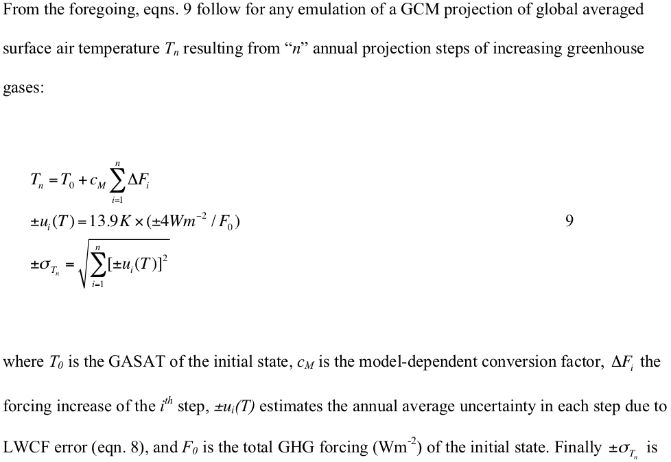
And why annual, when GCMs have steps of 30 minutes? It comes back to that averaging nonsense. He averaged 20 years of data, and said the average was 4 W/m2/year, not 4 W/m2. If he had expressed it as averaging 240 months of data, he would have taken monthly steps, and compounded the error at sqrt(12) times the rate.
Nick Stokes, “He’s saying that successive time intervals contribute independent errors with sd 4.”
No, I’m not. I’m saying that uncertainty increases, not that error increases.
The error of a future time state is entirely unknown.
You’ve made mistakes 2, 4, and 6 again.
Nick, “He averaged 20 years of data, and said the average was 4 W/m2/year, not 4 W/m2.”
I did no such thing. Serious mistake, Nick. And you claimed to have read the paper.
I averaged no set of data. Lauer and Hamilton averaged data, not me.
They calculated the 20-year annual mean calibration error statistic made by their set of 27 CMIP5 models.
Their 20-year annual average ensemble mean bias (eqn. 1) was calculated as delta = (1/N)[sum over N of (model minus observed).
Guess the dimension of the 1/N divisor. Does that dimension enter the dividend?
I took their rms annual average long-wave cloud forcing error statistic. They reported that as ±4 Wm^-2 annual average = ±4 Wm^-2year^-1.
It’s a statistical average, Nick. Not a measurement average.
Statistical averages are of dimension (property average)/(unit averaged). The average height of people in a room is meters/person, not meters.
Twenty calibration error magnitudes averaged over 20 years is annual average error is error/year. Multiply by twenty, recover the sum.
Your assessment is utterly wrong (again).
wat
Benjamin ….. exactly
Back to middle school math for you, Benjamin Winchester, and take Toneb with you.
Nick Stokes, “annual steps. Well, OK, could be anything. It’s just a fit PF has chosen. You could have any step length.”
Air temperature projections are published as annual time series. The CMIP5 LWCF calibration error statistic of Lauer and Hamilton is an annual rms average. Those realities completely justify my choices.
Nick, “[GCMs] don’t have annual steps. They have steps of about 30min. That is about n=1.75e6 steps in a century, or ±419°C. ”
Nick supposes the LWCF calibration error statistic for 30 minutes is the same as for one year. Pretty naïve mistake, Nick.
Nick, “It’s a claimed error in the identification of TCF.” It’s a measured and published simulation error. No one claimed anything. Except you.
Nick, “doesn’t switch between ±4 W/m2 every 30 mins, or even every year. But the error is calculated as if it did.”
It’s not error, Nick. It’s an uncertainty statistic. Mistakes 2, 4, 5 and 6. You’re out.
Nick, “If it ever did wander by 15°C or 419°C, that would greatly change energy balance”
You’re treating an uncertainty as a physical temperature and a calibration uncertainty statistic as an energetic perturbation on the model. Mistakes 2, 11, and implicitly 12. Seriously fatal mistakes.
In fact each of your mistakes is fatal, Nick.
Your analysis is wrong throughout.
Indeed, your analysis is so clueless it doesn’t even rise to wrong.
“Air temperature projections are published as annual time series. The CMIP5 LWCF calibration error statistic of Lauer and Hamilton is an annual rms average. Those realities completely justify my choices.”
That is nonsensical reasoning. Your results are entirely dependent on the time step. If you have 100 steps, you multiply by sqrt(100). If you have 1000, you would multiply by sqrt(1000). Sp you are telling us that the whole magnitude of your estimated error is dependent on arbitrary publishing conventions.
You have committed errors 0, 7, 32 and 77. Average error score 29 sec^-1. You didn’t last long long.
Nick Stokes “Your results are entirely dependent on the time step.”
No, they’re not. You’re assuming that the average annual ±4 Wm^2/year LWCF calibration error is invariant with the averaging interval.
I dealt with that in ESS Round 1 reviewer 4, item 4.
If the averaging interval changes, so does the calibration error value. Put those new values into the error propagation equation, and a completely comparable uncertainty comes out.
The centennial projection uncertainty is about ±15 K no matter what.
I’m horrified allegedly qualified scientists don’t know what error is.
Allegedly. Ah yes, only Pat Frank does.
You certainly don’t Nick. The evidence for that is fully in view above.
By the way, my perception of error is taken from the literature. One can read all about it in Sections 7 and 10 of my Supporting Information document. You did read that, too, didn’t you Nick.
They know. They just don’t care.
They know, which is why Pat Frank’s paper keeps getting rejected.
Excellent article.
This is precisely where we need to focus.
Iterative models exlode even the tiniest errors and faster computers just generate garbage faster.
I will definitely be downloading and propagating this.
You ask – at 2:52 am in the same time zone that Willis is in.
Some of us need a night’s sleep now and again.
Hello Pat,
I am no scientist, although I did love learning about Geology & as well as watching the stars.
Keep your head held high and hold to what you believe is true.
One of my favourite sayings, ‘To thine own self be true.
Sandra
Thanks, Sandra. 🙂
If models are moving away from linear propagation of everything to more life-like nonlinear behaviour, involving a mix of positive and negative feedbacks – then that is a move in the right direction.
Haha Oh Pat Frank, you’ve lost the plot here.
“The stakes are just too great. It’s not the trillions of dollars that would be lost to sustainability troughers. Nope. It’s that if the analysis were published, the career of every single climate modeler would go down the tubes, starting with James Hansen. ”
I actually showed your work to a friend of mine who work on climate models. He was not impressed. Sloppy math. That’s all there is to it. No massive conspiracy that you could singlehandedly expose IF ONLY they’d publish it in the peer reviewed corner of the internet rather then the WUWT corner.
Cheers
Ben
So show us an example of the the “Sloppy Math” !! Or do you just do Drive By Whining ?
So why doesn’t your “friend” come and comment on it if you don’t understand the math? It seems, from the evidence, that anyone who works on models could use all the ideas for improvement they could get, seeing that not one of them can produce anything that looks like reality!
john, it’s hard to get imaginary friends to interact with real people in the real world.
A climate modeler rejects criticism of his models.
Color me surprised.
LOL!
I have a mate who knows a mate…who knows something about ……errr….what are we talking about again?
He knows a guy… Is this an “Ocean’s 11” reference?
There was one time, at band camp, when a climate modeller showed me his math…..oh boy, did all us girls have a laugh!
sloppy math guys, that’s all there is to it. Should be pretty clear from the text I quoted that the authors has completely and utterly lost perspective. Perhaps Pat Frank would do us all the favour of publishing the complete review comments of every time the paper was rejected, rather than selectively quoting and commenting? That would actually be interesting.
The full review comments are linked right there in my essay, benben. All 44.6 MB of zip file. Have at them. The link is just above the 12 points of reviewer scientific acuity.
And as John, Butch and bitchilly wrote, do bring your friend around for a conversation.
benben said “goo-goo” and “waah-waah”. !!
Many more people have access to WUWT than most climate pal-reviewed papers EVER get.
Heck , even benben could go ga-ga over it, if benben was capable..
” more people have access to WUWT than….”
…
Andy, please do not confuse quantity with quality.
Mark S
Are you saying something about the 97%?
Yes, I know YOU lack any sort of quality.
But many people here have more maths and science training than most so-called climate scientists.
You are just not intelligent enough to realise that.
You can catch with Willis here:
https://rosebyanyothernameblog.wordpress.com/
If someone tried to include a climate model as part of a nuclear power plant safety evaluation … such as “this climate model says the local temperature 40 years from now will be X and ocean levels will be Y so that’s what the nuclear plant design will be based on” … they would be laughed at by the nuclear regulators (whose employer funds climate models lol) and the nuclear plant investors.
Engineers and nuclear regulators understand climate models are primarily political constructs and not something that can be relied on for engineering. If climate models can’t be relied on for engineering purposes, then they are junk.
Just one example of the sheer nuttiness here. ESS reviewer 1 objected very reasonably:
“The dimension of +-4 W m-2 year-1 is not right, but should be +-4 W m-2, since it
is calculated from 20-yr means but not 20-yr trend. The author lacks basic knowledge on averaging.”
So for this he copped a tirade. But he’s obviously right. The PF deatiled response refers to Eq 6.2:

If you average 20 years of temperature, you get an average as T°C. It isn’t T°C/year, just because you had 20 years. You could average the same as over 240 months. That doesn’t make it T°C/month. And it isn’t just a typo. He has altered the text to make the claim clearer. The units are repeated many times, and the issue is central to the error calculation.
Eq 6.2 – sorry, Sec 6.2.
So, according to my understanding, this annual average of the cloud coverage as an input of a climatic model is decent. It looks different if one assumes that the average, which does not include a trend, is for the future. But as an input for a simple model, this is not objectionable for me. Except one searches for any grounds for a complete rejection of the model. There are many averages that are broken down in the year, in other scientific branches, why should this average be wrong: during the period mentioned, the heat input was so high. Now he is broken down annually.
For example, a company has been operating excellently over the last 20 years, with the exception of the last two years. Then came the proceeds. What was due to restrictive politics and data grief, especially the Middle Kingdom. If one now assumes that a newly elected President Trump would bring it to an end (which he has not normally done yet) to change this policy and end this data gag, the prospects for the company look the same much better. Therefore it is wrong to conclude from a relatively short period of the data on the further trends. In this case, an observation of the company’s healthy base would be more meaningful for the entire period.
Nick Stokes
L&H Table 4 is satellite measurement uncertainty, not model error. That is irrelevant to the argument.
L&H Figure 2 shows “the ensemble mean bias of the CMIP3 and CMIP5 models., i.e., the difference errors between model simulations and observations.
Figure 2 does not reference one simulation made N times.
It references N separate and distinct simulations.
For each of N models: simulation minus observation = error/model.
For each model, twenty years of simulation error, averaged annually = [Sum of (error/model)/20 years] = error/model/year.
rms of N-fold error/model/year = ±(error/model/year)
L&H began at the grid-point level, meaning positive and negative errors were derived. The reported rms ±(calibration error) was global annual.
You’re making the same mistake Patrick Brown did in the discussion we had on his presentation page, supported by ATTP and reinvented by my ESS reviewer.
You’re forcing the units of a measurement average (magnitude) onto a statistical average (magnitude per unit). You’re wrong.
Still, on average you will see T°C each(!) year. Would you calculate with an offset of T°C to estimate the temperature in 20 years or would you calculate 20 x T°C?
That’s basically what he is saying.
But what temperature do you want to take 20xT? the first, the last or the average yearly temperature of a twenty-year period? The calculation of the model author is not bad as input. And it also includes a trend, which I have judged negatively in my previous post. No, I think reviewers are overwhelmingly in a climate of rejection. If you think about what Climategate has shown, which reviewers have the say in which circles, is not surprising. Since then, nothing has changed, even if someone has been forced out of his age, he was replaced adequately.
So change the time scale to months. Would you calculate 240 x T°C?
Everything is about the average / year. So once you define it as such you have to take it. To prove the author wrong you should debunk his calculation where he defines the +/- 4 W/m² as a yearly value.
Regarding your example with temperature. I understood it this way: You have a 20-yr. trend (!) in temperature. Let’s assume the temperature is rising T°C/year on average. Of course you have to apply T°C every year to estimate the temp. after 20 yrs. If you just had varying temperatures without any trend, then T = 0°C. Since the paper, the author was referring to, based its calculation on a 20-year trend I am assuming that
a: there is a trend 0
b: which implies there is a yearly contribution
it should be:
a: there is a trend greater or smaller than zero
[The mods note that, indeed, most trends are greater then, equal to, or less than zero. .mod]
I just checked Lauer and Hamilton, 2013. This is the paper, Pat Frank is referring to. As far as I can see they are talking about annual(!) means based on a 20-yr trend.
‘Figure 2 shows 20-yr annual means for liquid water path, total cloud amount, and ToA CF from satellite observations and the ensemble mean bias of the CMIP3 and CMIP5 models.’
It seems correct to use the yearly value, because Lauer & Hamilton are doing it as well.
http://journals.ametsoc.org/doi/pdf/10.1175/JCLI-D-12-00451.1
“As far as I can see they are talking about annual(!) means based on a 20-yr trend.”
There is nothing there about a trend. They are simply averaging 20 annual means, which does not change the units. And they give the result in Fig 2, eg for LCF, in W/m2, not W/m2/year which PF changes it into.
“Consider: (20-year sum of annual uncertainties)/20 years = uncertainty per year.”
When you average, you don’t divide by 20 years. You divide by 20 units. It doesn’t change the dimension.
Er… if the uncertainty doesn’t have a time dimension, over what period did the uncertainty accumulate? Very little happens over zero time in any physical process to generate uncertainty.
paulclim is correct, the correct step seems to be one year.
Nick, First, L&H Figure 2 shows annual differences. Annual differences, Nick.
Do they really have to put “per year” on those numbers for a reader (you) to figure out that “20-year annual averages” are magnitude per year?
Figure 2 does not show L&H’s root-mean-square LWCF annual average statistical error, which is what I used.
Pat,

“Nick, First, L&H Figure 2 shows annual differences. Annual differences, Nick.”
Complete nonsense. The caption to Fig 2 says:
“FIG. 2. Differences in (top to bottom) 20-yr annual averages of LWP, CA, SCF, and LCF from the (left) CMIP3 and (middle) CMIP5 multimodel means compared with (right) satellite observations. For details, see text.”
They show differences between the 20 year averages of multimodel means compared with 20 year annual averages of satellite measured. Nothing about annual differences. And they mark the result as W/m2. They are scientists; they get units right. Here is the bottom frame and caption:
They spell it out for Fig 1:
“Figure 1 shows the 20-yr annual mean liquid water path averaged over the years 1986–2005 from 24 CMIP5 models that have LWP as an available variable.”
When they give error estimates, they express them generally as %. That is, % of W/m2. Here is Table 4, which does give a unit for LCF too. That unit is W/m2. There is not a unit W/m2/year anywhere in the paper.

I think the term error / year is misleading. If you take it word by word it leads to Nick’s interpretation which is correct because the error of the model is constant over time. But I think that’s not the dispute.
The question is how does this error behave in terms of uncertainties when modelling a non constant CO2 forcing. Let’s assume the time interval of the model is a year and the starting CO2 forcing is 4 W/m² and the error also is +/-4 W/m². The next year the CO2-forcing will be 4.035 W/m² due to slightly risen CO2 concentration and the error will still be 4 W/m². That delivers a band of statistically possible temperatures in the second year which means the uncertainty in the 3rd year will be even bigger because now you have to apply the model error to the results of the first loop which are inputs to the second. That’s the propagation of a constant error.
I don’t see a problem with computing a SD from 20 consecutive annual numbers each of which happens to be either averages or difference scores (which themselves were computed from averages and a reference point) from the same instrument.
If the numbers are from totally different sources (year to year changes in the underlying effect might qualify), one would have to weight the 20-year mean by incorporating the variability in each of the underlying annual averages; and the variance in the 20-year mean would be a function of the variance within each source (year to year) – each annual average should have a variance.
No need to worry about a trend, because 1) the aim is a conceptual 20 year average, and 2) the trend is conceptualized as diffferent effect sizes for each year.
Nick Stokes “There is not a unit W/m2/year anywhere in the paper.”
My bolding throughout.
Page 3831, column 1: “Interestingly, BCCCSM1.1, CCSM4, and NorESMl-M show similar biases in the simulated annual mean LWP,…”
Annual mean bias = error/year
Page 3831, column 2: “Figure 2 shows 20-yr annual means for liquid water path, total cloud amount, and ToA CF from satellite observations and the ensemble mean bias…”
Ensemble annual mean bias = average error/model/year
Page 3833, column 1: Taylor diagram “comparisons of the annual mean cloud properties with observations” giving the “standard deviation … of the total spatial variability calculated from 20-yr annual means.”
In the Taylor diagram, “the linear distance between the observations and each model is proportional to the root-mean-square error (rmse)”
That’s the root-mean-square error (rmse) of the 20-year annual means = error/year.
All the errors (biases) quoted are in reference to 20-year annual means. All of them are rmse.
Page 3833, “For CMIP5, the correlation of the multimodel mean LCF is 0.93 (rmse = 4 W m^-2) and ranges between 0.70 and 0.92 (rmse = 4–11 W m^-2) for the individual models.” LCF is long wave cloud forcing, simulation of which produced the calibration error statistic used in my analysis.
Multimodel average LWCF rmse of 20-year annual means is ±4 Wm^-2/model/year.
L&H may not write it that way, but it’s very clear from the usage in the text, and from the meaning of their equation 1, that that is exactly what they are reporting.
Pat,
“L&H may not write it that way, but it’s very clear from the usage in the text, and from the meaning of their equation 1, that that is exactly what they are reporting.”
It is only clear to you. Normal folks see 4 W/m2 and take it that they mean 4 W/m2.
All the annual mean qualifiers that you bolded are just there to emphasise that seasonal effects are removed. Annual means are themselves made up of readings during the year, which are averaged. You described the process here

But the units are now simply cloud-cover, not /measure or /week or whatever. No change. Yet when you further average those annual averages in 6.4, you change the units to /year. It makes no sense.
Nick Stokes, eqn. 6-3 shows the 20-year mean observed cloud cover bringing in the average over the year and dimension year^-1.
Eqn. 6-4 does the same for simulated cloud cover.
As soon as you take a 20-year mean, the dimension of the dividend acquires year^-1.
Pat,
“As soon as you take a 20-year mean, the dimension of the dividend acquires year^-1.”
So why don’t units change in 6.2? Why is it different averaging over sub-year intervals?
If you take rms, do they acquire year^-0.5?
Nick is right. Annual means means average over a year in this context. It would be different, if there were a trend, i.e. a growing error over 20 years. In this case you could read it as error/year. But that is not the case because over 20 years the total error would be 80 W/m2 which is more than the observation. So most likely annual means has to be read as average over a year and a 20 year average of annual means most likely is the average of 240 consecutive months.
Nick Stokes, “So why don’t units change in 6.2? Why is it different averaging over sub-year intervals?”
Why should units change in eqn. 6-2? Change from what?
Equation 6-2 is step 1 applied to cloud cover expectation values. It averages them at a given grid point within a given year. It has the same dimensions as eqn. 6-1.
Nick, “If you take rms, do they acquire year^-0.5?”
Different time averages acquire their own dimensions and error values. I worked with those of L&H. The dimensions are consistent throughout.
paulclim/a>, “Nick is right. Annual means means average over a year in this context. It would be different, if there were a trend, i.e. a growing error over 20 years. In this case you could read it as error/year. But that is not the case because over 20 years the total error would be 80 W/m2 which is more than the observation. ”
L&H report a calibration experiment. Calibration error statistics do not require a trend. They require consistent dimensional units. One could take the model LWCF error from multiple individual years and combine them into a calibration annual error statistic, and it would be of dimension W/m^2/year.
Calibration error is not a slope.
Further, your “80 W/m^2” is the result of treating the ±4 W/m^2 as a physical error, rather than a statistical uncertainty. ±4 W/m^2 is not the slope of a trend.
You have also dropped the “±” in your analysis. I.e., you should have written, “ total error would be ±80 W/m2.”
How can a slope be “±”?
Is ±80W/m^2 more than the observation? When can a physical error value be simultaneously plus and minus?
Never, obviously. The “±” is a dead-obvious statistical give-away.
The L&H 20 year annual mean is across 1986-2005.
Nick is wrong.
Sorry for not closing the html link
Pat,

“Why should units change in eqn. 6-2? Change from what?”
I don’t think they should. But again, here is 6.2
You are averaging cloud cover over n periods in a year. Yet the result is still in cloud cover units, with nothing in the denominator. Yet when in the almost identical next stage

you average cloud cover over N years. Then you say it must be expressed as CC units/year.
What if you had just averaged the n*N readings in one sum? If n is the same for each year, you’d get the same numerical result. What would then be the units?
Nick Stokes, “What if you had just averaged the n*N readings in one sum? If n is the same for each year, you’d get the same numerical result. What would then be the units? ”
Averaged “n*N readings in one sum” over what unit-time scale? Choose your scale. Do the dimensional analysis. Let us know.
OK, suppose the n readings per year were monthly. So you average over 240 months. Same numerical answer. Are the units CC/year or CC/month.
Or again, for the 20 annual averages, what if you averaged the first decade, then the second, and then averaged the two decades. Again, same numerical answer. Are the units CC/year or CC/decade?
Nick Stokes, “suppose the n readings per year were monthly. So you average over 240 months. Same numerical answer. Are the units CC/year or CC/month.”
Sorry for the delayed response. Just back from travel, and opportunities were limited.
But let’s parse your question, shall we?
Start with a monthly average of CC across a year as (sum of all 12 monthly aggregated observations/12). We have average CC that year. The average CC for that year is CC/month isn’t it.
Every month of the annual average now has identical CC, from Jan. through Dec.; the uniformity of CC imposed by the averaging process.
But why stop there? Average 365 days of CC. Every day of the resulting yearly average also has the identical average CC value. And that daily average CC/day value is identical to the CC/month value of the previously monthly averaged year. Is the new average dimensioned CC/day? Even though it’s identical in numerical value to the CC/month?
How did CC/month transmogrify into CC/day?
How about averaging the CC every minute of every day of every month for the entire year. The same identical average CC value. Is the average dimension CC/minute, or not? Surprise of surprises, CC/minute value = CC/month value.
Is it confusing that the yearly averaged CC has the same numerical value at 1 minute as it does at 1 year?
The way out of the conundrum is to realize that the uniformity of CC average value at all subordinate time scales is imposed by an averaging process that extends across the year.
An annual averaged CC has some physical meaning if one wanted to compare annual average CC year-by-year, to look for annually significant changes.
The CC/minute value obtained from an annual average has no physical meaning. Comparison of minute 1, January 1 of annually averaged year 1 with minute 1, January 1 of annually averaged year 2 is physical nonsense.
The CC average value of a minute has no meaning taken from an annual average of CC.
The same discriminatory logic applies to your 240 month average. The 240 month averaged CC is of uniform intensity across that entire time at all internal time scales. Across the 240 year avarage, CC/second = CC/month = CC/year, imposed by the averaging process.
What would be the physical meaning of the 240 month average CC at one second resolution, or one month?
So, the answer to your opening question is ‘yes.’ But taking an average imposes uniformity of value across the averaged metric. The smaller dimensionality denominators are numerically valid but physically meaningless.
There’s a distinction that goes to the heart of your continual misperceptions about physical error analysis, Nick.
The CC/month of a 240 month average has no physical meaning, except on a 240 month scale, and perhaps in the context of comparing alternative 240 month averages. The significance is at 240 months, not one month. The uniformity of CC value at all internal subordinate time scales is a numerical artifact of the method; one that has no particular physical significance.
No one would be particularly interested in seeing how a 240 month average changed in terms of CC/month because over a 240 month time range, the imposed monthly denominator transmits a false claim of resolution. It has negligible physical meaning.
Now let’s look again at the L&H error metric.
Let L&H calculate twenty annual errors as annual (CC_mod – CC_obs). Then sum up the 20 differences, and divide by 20. The unambiguous result is an annual average error, of denominator year^-1.
That error is identical to the one obtained by separately averaging 20 annual CC_mod and 20 annual CC_obs.This yields CC_mean-mod and CC_mean-obs. Their difference produces the ideintical annual average error. The same per annum (year^-1) is physically meaningful because the annual resolution is physically real.
The reason is that each annual CC_mod and each annual CC_obs was physically unique. Their 20-year annual average therefore has physical meaning as an annual average of denominator year^-1.
Following from the above, L&H would also have a physically meaningless but numerically identical per month average error and a per second average error.
Those error metrics are physically meaningless because the resolution of the average does not produce physically valid individual months or individual seconds.
That completes the resolution of your posed numerical conundrum.
It’s interesting to note that if the satellite observations were sufficiently numerous and regularly spaced across every month of the 20-year experimental range, a per month rms LWCF CMIP5 model simulation calibration error statistic could conceivably be calculated.
It would probably not be ±4 W/m^2, but whatever it turned out to be could be propagated in monthly steps rather than annual steps, across an air temperature projection.
Whatever the centennial temperature uncertainty turned out to be, I have no doubt but that its message would be identical to that conveyed by the annual propagation. The one that yielded about ±15 K. The meaning is that air temperature projections are entirely unreliable right up through the CMIP5 versions of them.
Pat,
“Is it confusing that the yearly averaged CC has the same numerical value at 1 minute as it does at 1 year?”
Well, very little of what you said makes sense. But let’s make it really simple. Suppose you measure the temperature of a location every day for 20 years. And it turns out, unexpectedly, that it’s a location with constant temperature, 24°C.
So you average the days of every year, then average the 20 years. 24°C/year. Yes?
Or you average the days of every month, then average the 240 months. 24°C/month. Yes?
You and Forrest spoke learnedly earlier about dimensional analysis. In any such system, 24°C/year is 2°C/month. It has to be, if dimensions mean anything.
So what gives?
If it was a vector, you’d be right, its not, its a scalar.
Vector/scalar has nothing to do with dimensions. The magnitude of a vector is a scalar, but has the same dimensions.
It’s the differences between a rate and a scalar. If it was 24°/yr as a rate change, it would be 2°/month, but it’s not a rate! How hard is that for you to understand? And while they have the same dimension(but hold on), its not the same units. Ie 24°/yr change, vs 24° average/year.
So really they don’t have the same dimensions.
“differences between a rate and a scalar”
This is getting very muddled. rate and scalar are not opposites. 24°C/year could be a rate and is a scalar. But units are units. Dimensions are dimensions. They don’t embody any extra meanings like whether rate or not.
But that’s just it, they are not the same dimension, you’re describing delta T/time period vs Avg T/time period, they are not the same thing!
Nick Stokes, “Well, very little of what you said makes sense.”
Meaning only that you understood very little of what I wrote.
I pointed out that averaging across long times imposes the numerical uniformity that confuses you.
However, your present example is even more confused. You begin by proposing a site of constant 24°. Constant 24° means a reading every second will register 24°. Averaging per second then yields 24°/second, too, Nick.
This 24°-no-matter-the-unit-dimension is identical to the conundrum I resolved in my prior post. The one you didn’t understand.
What makes your current example more confused than your previous one is that the constant 24°/(dimension of your choice) is a direct consequence of your built-in assumption of constant 24°.
Bottom line is that your system of constant 24° yields 24°/year, 24°/month, 24°/second, and 24°/(internal duration of your choice). That’s the physical meaning derived from your own assumption. Your numerical playing about produces physical nonsense.
For example, for what physical reason would one divide a constant 24°/year by 12 months, when it is known that the temperature during every one of those months was 24°? The answer is: no physical reason at all.
Your division by 12 is physically meaningless, making your 2°/month physically meaningless. What is the dimensional meaning of a physically meaningless construct?
Dimensional analysis doesn’t mean making physically nonsensical algebraic ploys. It means tracking dimensions through a calculation to be sure the final dimension is correct with respect to the equations used.
Nick, this quote from Einstein, from the Stanford University Online Encyclopedia may help you understand that the way to think within the physical sciences is different from your numerical consistency.
Physical meaning must, and always does, take precedence over philosophical (numerological) formalities.
“The reciprocal relationship of epistemology and science is of noteworthy kind. They are dependent upon each other. Epistemology without contact with science becomes an empty scheme. Science without epistemology is—insofar as it is thinkable at all—primitive and muddled.
“However, no sooner has the epistemologist, who is seeking a clear system, fought his way through to such a system, than he is inclined to interpret the thought-content of science in the sense of his system and to reject whatever does not fit into his system. The scientist, however, cannot afford to carry his striving for epistemological systematic that far.
“He accepts gratefully the epistemological conceptual analysis; but the external conditions, which are set for him by the facts of experience, do not permit him to let himself be too much restricted in the construction of his conceptual world by the adherence to an epistemological system.
“He therefore must appear to the systematic epistemologist as a type of unscrupulous opportunist: he appears as realist insofar as he seeks to describe a world independent of the acts of perception; as idealist insofar as he looks upon the concepts and theories as free inventions of the human spirit (not logically derivable from what is empirically given); as positivist insofar as he considers his concepts and theories justified only to the extent to which they furnish a logical representation of relations among sensory experiences (my bold).
“He may even appear as Platonist or Pythagorean insofar as he considers the viewpoint of logical simplicity as an indispensable and effective tool of his research.
(Einstein 1949, 683–684)
Note the sentence, “Epistemology without contact with science becomes an empty scheme.”
That empty scheme produced your 2°/month.
Contact with science shows your 2°/month is physically meaningless.
“But that’s just it, they are not the same dimension, you’re describing delta T/time period vs Avg T/time period, they are not the same thing!”
This, and Pat’s stuff, is just nuts, at a basic level. Quantities have dimensions and corresponding units. It’s as simple as that. The dimensions don’t depend on why you are calculating it, whether someone thinks you should have been calculating it, whether it is constant, or whatever.
And there are simple rules relating dimensions and units. If X is 24 units/year, then it is 2 units/month. It doesn’t matter what kind of thing X is or what “units” are. 1 m/sec is 1000 mm/sec is 3.6 km/hr. You don’t have to ask further questions in making those conversions. You can look them up from tables. Or Google.
The problem isn’t that it accumulated 24 units/year, it’s an average quantity of 24units/year, not the same thing.
The difference of standing in a creek that’s 24″ deep, and one that’s normally empty, until it storms and swells to 24″, and then drains.
Nick Stokes, “This, and Pat’s stuff, is just nuts, at a basic level.”
No it’s not. micro6500 is right. Your October 31, 2017 at 9:30 pm post and prior treat 24°C/month as the slope of a trend, when it’s the average of quantities (in your example, of a constant over time).
“Quantities have dimensions and corresponding units. It’s as simple as that. The dimensions don’t depend on why you are calculating it,…”
The physical meaning is the crux of the issue. That meaning depends on the physics of the system, Nick. Your usage is physically meaningless.
Slopes and statistical averages have the same dimensional form: magnitude/unit. But the one is not the other, physically. You have consistently and incorrectly conflated them. So did my reviewer.
When you first began this line of questioning, I thought you might be trying to pose a trick question. Now I see that I was wrong. You plain don’t understand what you’re doing, Nick.
Just as in your confused view that instruments of measure have infinite resolution.
Nick is correct, though. The 4 W/m^2 is the multi-model mean spatial root-mean-square-error of longwave cloud forcing between models and observations calculated over 20 years (I think the citation is Lauer & Hamilton, 2012). It is not 4W/m^2/yr, it is simply 4W/m^2.
I showed that revised Sec 6.2 from the SI.
“Consider: (20-year sum of annual uncertainties)/20 years = uncertainty per year.”
When you average, you don’t divide by 20 years. You divide by 20 units. It doesn’t change the dimension. If you average your weight over a year, it doesn’t come out as kg/year. If you average over 12 months, it isn’t kg/month. That’s elementary. Yet PF makes a big issue of it.
“Consider: (20-year sum of annual uncertainties)/20 years = uncertainty per year.”
When you average, you don’t divide by 20 years. You divide by 20 units. It doesn’t change the dimension.
Er… if the uncertainty doesn’t have a time dimension, when did the uncertainly accumulate? Very little happens over zero time in any physical process to generate uncertainty.
paulclim is correct, the correct step seems to be one year.
(sorry, wrong subthread)
“Instead you went for the smear.”
Wow. I said his misuse of averaging was nuts. It is.
So what do we get from Pat Frank
“It’s not the trillions of dollars that would be lost to sustainability troughers.”
“Given all that conflict of interest, what consensus climate scientist could possibly provide a dispassionate review?”
“As a monument to the extraordinary incompetence that reigns in the field of consensus climate science”
” a noxious betrayal of science by the very people charged with its protection.”
And then to the editor of Journal of Climate
“So how does it work, Tim — are you truly so dishonest, or merely stampeded into cowardice?
You must know very well manuscript JCLI-D-15-0797 is correct.
And that the reviews are incompetent.
When did science become the willful suppression of valid criticism?
When did science countenance a conscious defense of the false?
When did wrong become privileged?
When you sit at your desk, wouldn’t professional dishonesty rob your life of meaning and purpose?
Yours sincerely,
Pat Frank”
Nick,
Your citation (sec. 6.2) notes that that Cug has dimensions of ‘mean cloud cover unit per year yet you insist that the dimension does not include ‘per year’.
Also, you have cited examples of averages where the ‘per unit’ (year, month, day) dimension does not apply yet your citation is a mathematical average and it is defined having dimensions of ‘per year’. Please explain.
ATTP, you describe the variable in question as being a “multi-model mean spatial root-mean-square-error”. The equation cited by Nick, sec 6.2, is a simple average; giving it a fancy name doesn’t change that but it may intimidate those who don’t recognize the form of the equation. Nice try but still a FAIL.
Ray,
“Your citation (sec. 6.2) notes that that Cug has dimensions of ‘mean cloud cover unit per year yet you insist that the dimension does not include ‘per year’.”
I’ll show the original citation again

Says the result of simple averaging, Cug, has units cloud cover/year. It doesn’t spell out the units of the thing averaged, Ckg, but it refers to Eq 6.2 as the origin. Here is eq 6.2:

Dimension cloud cover unit, not per year. Bizarrely, that expression is also an average over sub-units of time in a year, but does not acquire a per time unit.
“The equation cited by Nick, sec 6.2, is a simple average; “
Yes. It isn’t what ATTP is talking about, but that is all it is. And yet, as the ref said, he got it wrong. And it matters because it is where the notion that errors have to be compounded annually came from.
Nick Stokes, “Bizarrely, that expression is also an average over sub-units of time in a year, but does not acquire a per time unit.”
It’s pretty simple Nick. Eqn. S6-1 and S6-2 provide the average of cloud cover per grid-point in each given year.
The number of simulated cloud cover values per given year need not match the number of observations per given year.
Eqns. S6-1 and S6-2 sum up the observed or simulated values, respectively, in each given year and take the average magnitude for that year.
Simulated and observed cloud cover units must eventually have identical time scales, in order to make the difference in eqn. S6-5. Hence conversion to the uniformly annual scale.
The equations are not time averages. They are number averages. Any time sub-unit (simulation time-step; observational time interval) is lost because the number average scales to the annum in each given year.
It really is that simple, despite the complicated hash you’re trying to make of it.
I think the real source of the problem you’re having is in dealing with gritty Galilean physics while being trained to Socratic idealism.
Adding: Nick Stokes, “And yet, as the ref said, he got it wrong. ”
No, Nick. The ref got it wrong, and so have you (and ATTP).
The metrics are key to at least part of the discussion. Get the metrics right first.
Jan says it well. There are different kinds of error: experimental errors are inherent in the result and have to be propagated through subsequent calculations. Systematic errors (using an incorrect forcing value) can be identified which means corrected. The ISO has a lot on GUM and standard reporting structures for it. There is no way climate model outputs are ISO compliant because they do not properly report the propagated uncertainties. They treat the calculated number as golden perfection.
Nick has persistently indicated he doesn’t think uncertainties propagate.
The question of an uncertainty per year is interesting. If at the beginning there is no uncertainty at all one has perfect measurements or perfect assumptions. Fine, let’s presume that is the case. After 1 year there is an uncertainty of 4W/m^2 it can stand alone. If that model is run for another year carrying an uncertainty about the ‘inputs that arises from Year 1, that uncertainty has to be propagated through year two.
Suppose the uncertainty were assessed after 30 minutes of model run, (starting with perfect inputs). Whatever uncertainty arises comes from what exactly? Doesn’t matter. Black box it.
The big problem is the misunderstanding that a range of modeled results does not represent the uncertainty about the answers. The propagation of error (uncertainty – look it up) goes with each calculated output. So what I see above is aTTP trying to sell variability of model outputs as the uncertainty attached to each result. I am not sure who is convinced by such a misrepresentation. One might get 1000 different model results that were 100% certain as to their value. There is a fundamental difference between the range of results and the uncertainty of each result, which depends on the uncertainty of the measurements/inputs.
Michael Mann produced a mathematical calculation that assembled a lot of tree ring data to produce a proxy temperature series. Whatever date was fed in from any set of trees, the result was always a (rather convenient) hockey stick shape. This is an example of a mathematical process in which large differences are observed in the inputs, but the result was always the same. In such a case the variability in the result is small. Mann’s results were quite non-varying. That in no way means his results were ‘certain’.
Crispin,
“They treat the calculated number as golden perfection.”
As they should. They are reporting a calculation, and the only relevant error would be machine rounding. The point of an error estimate is that it tells you the range of results you might have got if different circumstances had affected the measurement. Different instruments, different temperature, different observers etc. But with a model calculation, you don’t have to speculate. You can do it again and again with those changes, and actually see the range of results you get. That is the point of an ensemble.
“There is a fundamental difference between the range of results and the uncertainty of each result, which depends on the uncertainty of the measurements/inputs.”
No, again the uncertainty is actually just an estimate of the actual range of results you might get if the inputs varied over a range of uncertainty. That’s why an ensemble is the proper way to work it out. It’s always possible that not everything that should be varied will be, but the same is true of any error estimate.
What you won’t see is the IPCC or similar presenting just one model result and saying that this is golden perfection. They always present a range. OK, Hansen 1988 was an exception, but that was because they only had one. You have to start somewhere.
If you average 20 years of model temperature error, you get error/year.
Magnitude average vs. statistical average, Nick. You’ve got no idea. Neither did that reviewer.
As Forrest Gardener noted, you quoted the reviewer as though his view were definitive, without addressing my reply. That’s to lie by omission, isn’t it.
That reviewer also did not realize that one need not have a trend of calibration measurements to combine them into a calibration error statistic. The calibrations need only reference the same instrument, method, and conditions.
That reviewer implicitly assumed the statistic dimension, property/unit, is a slope. it’s not.
Pat,

“Magnitude average vs. statistical average, Nick.”
Gobbledygook. There is only one kind of average, and you spelt it out here
And it does not somehow acquire new units. If you average your height over 20 years, you get height in feet. Not feet/year. If you average the annual averages of your height, you get the same answer. And in feet.
The mean of 20 annual-average-errors is both the mean annual-average-error and the average-error per year. They are one and the same.
RW: i see
you didn’t respond
to the comments
I made today in reply
to yours.
crackers345: I didn’t see them until now.
If I average the change in my height over 20 years it’s inches per year. Nick.
And the errors recorded in L&H are likewise differences over time.
Thank-you for quoting my final email, to Tim DelSole Nick.
I invite everyone to read the two J. Clim. reviews and my responses. Between them, the two reviewers made pretty much every one of the 12 mistakes listed in the head post.
They are utterly incompetent.
Review #1 was so poor as to suggest the reviewer never critically read the paper at all.
Reviewer #2, among other fatal mistakes, also inadvertently validated the analysis (giving you something in common with him, Nick).
Tim DelSole is a trained physicist. He should never have accepted those reviews. But he did.
He wrote, “On the basis of these reviews and my own evaluation, I am sorry to inform you that this manuscript is rejected.. (my bold)”
He rendered an independent review judgment but provided no reasoning. In view of the incompetent reviews, his rejection stands without justification.
His decision amounts to a star chamber proceeding.
You’re right. I was angry. The whole thing is a profound betrayal of science.
Consensus climate science is a parody. And its professional integrity is trashed.
And you support all of that, Nick, without knowing what you’re talking about.
Someone else who doesn’t know the difference between a magnitude average and a statistical average.
And who considers himself a scientist. Too funny. 🙂
Crispin, “They treat the calculated number as golden perfection.”
Nick, “As they should. They are reporting a calculation, and the only relevant error would be machine rounding.”
Thus spake the numerical modeler.
Nick’s comment ought to settle the case for every single physical scientist and engineer here.
Nick shows no awareness that the accuracy of calculations from physical models are conditioned by comparison with physical data.
But he wants us to know that he can critically evaluate physical error analysis. And ATTP supports him.
Incredible.
Yep, I have been watching. Its been quite funny to watch them both making exactly the same mistakes as the reviewer, all because of their complete lack of understanding about error propagation etc.
“Reviewer #2, among other fatal mistakes,”
The reviewer (J Clim) began thus:
“This manuscript is an impostor. It pretends to be a research paper, but it is not. A research paper makes a good-faith effort to provide relevant context as defined by prior work and then goes on to show how the prior work is extended (perhaps by showing flaws in it). By contrast, the present manuscript uses scientific-looking reasoning and referencing but blatantly ignores or misrepresents prior work. Furthermore, the manuscript contains fundamental errors in the technical development it claims to present as novel. Hence I cannot but recommend rejection.”
Sounds accurate to me.
” know the difference between a magnitude average and a statistical average.”
You just make this stuff up. So what is the difference? With references, please.
Using the weight example. So i weigh myself periodically, different scales, the numbers bounce around week to week. Maybe i got fat then slimmed down again over a monthly time frame and the measurements reflect that trend to some degree… I calculate the standard deviation over the year. In the absence of any other information, there isn’t a big problem applying the standard deviation to any single time point in the year. I do rely on the assumption that the errors are random and distributed Normal. I also rely on the assumption of homoscedasticity. That is, that the error, whatever shape it assumes, remains that shape across the trend; put yet snother way, that the errors are independent of the trend.
RW: you’re
confusing two
different
uncertainties — that of
the measurements, and
the statistical uncertainty.
crackers345. I rebutted the notion that an SD calculated across a time series cannot be expressed in the temporal units of the data. I might have posted in the wrong subthread though.
Nick Stokes “You just make this stuff up. So what is the difference? With references, please.”
Who needs references when a simple demonstration is available?
Several measurements of the height of one person: meters. A measurement average.
Average height of people in a room: meters per person. A statistical average.
Middle school math, and a numerical methods PhD stumbles over it.
Pat,
“meters. A measurement average.”
This was the distinction in question, quoting your words:
” know the difference between a magnitude average and a statistical average.”
Still wondering.
Although this was one for the ages:
“Average height of people in a room: meters per person. A statistical average.”
So if you have three thermometers in a room measuring temperature, and you average, does that make the result °C/thermometer?
Nick Stokes
Your example misses the crux.
Three thermometers in one room — presuming uniform air temperature throughout — are measuring a single variable. Average result in K. Magnitude average.
Three thermometers, one each in a separate beaker of water, each measuring a separate variable. Average result in K/beaker. Statistical average.
Same deal with the L&H simulations. They are not N versions of one simulation. They are N separate and distinct simulations. The average is a statistical average, not a magnitude average.
Pat,
“presuming uniform air temperature throughout — are measuring a single variable”
So the units depend on what you presume? What if you don’t know?
Should the average temperature of the US be in °C/thermometer?
Nick Stokes I was explicating the assumption hidden in your example.
If the temperatures in your example are not uniform across the room, then the average measurement would be K/measurement.
The differences from the average would be a ±K uncertainty in the temperature of the room.
So, without your hidden assumption, your example disproves your case.
In your US temperature case, the thermometers are not measuring a uniform variable. They’re measuring different variables — different local temperatures in different environments.
The uncertainty that applies in their average, apart from state variability, is the uncertainty due to field calibration error. Something I published about (870 KB pdf).
What is so hard about the distinction between combining repeat measurements of one thing, and combining many measurements of many things?
Pat
“In your US temperature case, the thermometers are not measuring a uniform variable.”
But the question is, what are the units of the US average T. Never mind he uncertainty at this stage. It sounds like on your definition they should be °F/thermometer. But what if they averaged states first. Is it °F/state?
Nick Stokes, it would all depend on scale, wouldn’t it.
L&H started out with error/grid-point for each model, didn’t they. They combined the errors to finally scale up to global average annual error, i.e., average annual error/globe.
You can choose any scale you like. Your final scale could be (average annual ⁰F)/(continental US), i.e., US annual average temperature in ⁰F.
Pat,
“Nick Stokes, it would all depend on scale, wouldn’t it.”
So it depends on uniformity (of temperature) and then scale. Sounds a lot to teach those middle-schoolers. But there is no consistency here. With heights in a room, you wanted to say the average was ft/person. Now you seem to want ft/room.
“L&H started out with error/grid-point for each model, didn’t they.”

Actually, no. They describe their model aggregation here:
Each x is an average of a quantity (not error) over 20 years. They then form the mean differences, which is their measure of discrepancy.
Forrest Gardener, your statements are equivalent. But in your first, the ‘per person’ is implicit rather than explicit.
If the average height of the people is 1.8 m, then the average height of all the people is 1.8 m/person.
More quantitatively, (sum of N heights)/(N people) = average height/person.
When doing some analysis quantitatively, one has to be explicit about the dimensional analysis of the equations used.
If intermediate dimensions do not cancel to leave only the proper dimensions of the final unit, then the equation is wrong.
Nick Stokes, “So it depends on uniformity (of temperature) and then scale.”
No. The central issue of your example was not uniformity of temperature, as you suggest, but whether the measurement is of a uniform system. Your “uniformity of temperature” conflates a single system at a single temperature with diverse systems at the same temperature.
They are not physically identical at all. Their averages are not the same either. The latter produces a statistical average.
Obviously the dimensional unit changes with the scale.
This isn’t “a lot to teach those middle-schoolers.” but it does seem to escape certain numerical modelers.
Nick, “But there is no consistency here. With heights in a room, you wanted to say the average was ft/person. Now you seem to want ft/room.”
You’re just pretending to be diversionary, aren’t you. Suppose you have 12 rooms, with 20 people per room. If you wanted an over all height average, why would it not be ht/person/room? You remember — as in W/m^2/year.
Nick, “Each x is an average of a quantity (not error) over 20 years. They then form the mean differences, which is their measure of discrepancy.”
Now you’ve stopped playing at it. I wrote that L&H began with the error per grid point. Their [x_i(mod) minus x(obs)] is an error metric.
You dispute that and now rename error as a “measure of discrepancy”, as though that were something different.
Get serious.
“It’s a long time since I did any dimensional analysis.”
Obviously. If you brush up on it, you’ll be reminded that
” dimensional analysis is the analysis of the relationships between different physical quantities by identifying their base quantities (such as length, mass, time, and electric charge) and units of measure (such as miles vs. kilometers, or pounds vs. kilograms vs. grams) and tracking these dimensions as calculations or comparisons are performed.”
“person” is not any kind of base quantity.
well maybe it matters when trying to compare against rooms full of virtual people who are getting added to some because they didn’t have enough with real people to measure.
When half your measurements average doesn’t even exist, maybe /thermometer should be added.
Nick Stokes ““person” is not any kind of base quantity.”
“person” does not designate an individual human being? Is Australian English (Strine) so degraded as to have lost the ability to assign simple meaning?
Forrest, you’re right. Apologies to you and Australia.
Nick, however, does grave disservice to your (his) nation.
Follow Willis on Twitter https://twitter.com/WEschenbach