We publish this here, not to confirm that it is correct, but to stimulate the debate needed to determine whether or not it is correct or if it’s simply an exercise in curve fitting. ~ctm
George White, August 2017
Climate science is the most controversial science of the modern era. A reason why the controversy has been so persistent is that those who accept the IPCC as the arbiter of climate science fail to recognize that a controversy even exists. Their rationalization is that the IPCC’s conclusions are presented as the result of a scientific consensus, therefore, the threshold for overturning them is so high, it can’t be met, especially by anyone who’s peer reviewed work isn’t published in a main stream climate science journal. Their universal reaction when presented with contraindicative evidence is that there’s no way it can be true, therefore, it deserves no consideration and whoever brought it up can be ignored while the catch22 makes it almost impossible to get contraindicative evidence into any main stream journal.
This prejudice is not limited to those with a limited understanding of the science, but is widespread among those who think they understand and even quite prevalent among notable scientists in the field. Anyone who has ever engaged in communications with an individual who has accepted the consensus conclusions has likely observed this bias, often accompanied with demeaning language presented with extreme self righteous indignation that you would dare question the ‘settled science’ of the consensus.
The Fix
Correcting broken science that’s been settled by a consensus is made more difficult by its support from recursive logic where the errors justify themselves by defining what the consensus believes. The best way forward is to establish a new consensus. This means not just falsifying beliefs that support the status quo, but more importantly, replacing those beliefs with something more definitively settled.
Since politics has taken sides, climate science has become driven by the rules of politics rather than the rules of science. Taking a page from how a political consensus arises, the two sides must first understand and acknowledge what they have in common before they can address where they differ.
Alarmists and deniers alike believe that CO2 is a greenhouse gas, that GHG gases contribute to making the surface warmer than it would be otherwise, that man is putting CO2 into the atmosphere and that the climate changes. The denier label used by alarmists applies to anyone who doesn’t accept everything the consensus believes with the implication being that truths supported by real science are also being denied. Surely, if one believes that CO2 isn’t a greenhouse gas, that man isn’t putting CO2 into the atmosphere, that GHG’s don’t contribute to surface warmth, that the climate isn’t changing or that the laws of physics don’t apply, they would be in denial, but few skeptics are that uninformed.
Most skeptics would agree that if there was significant anthropogenic warming, we should take steps to prepare for any consequences. This means applying rational risk management, where all influences of increased CO2 and a warming climate must be considered. Increased atmospheric CO2 means more raw materials for photosynthesis, which at the base of the food chain is the sustaining foundation for nearly all life on Earth. Greenhouse operators routinely increase CO2 concentrations to be much higher than ambient because it’s good for the plants and does no harm to people. Warmer temperatures also have benefits. If you ask anyone who’s not a winter sports enthusiast what their favorite season is, it will probably not be winter. If you have sufficient food and water, you can survive indefinitely in the warmest outdoor temperatures found on the planet. This isn’t true in the coldest places where at a minimum you also need clothes, fire, fuel and shelter.
While the differences between sides seems irreconcilable, there’s only one factor they disagree about and this is the basis for all other differences. While this disagreement is still insurmountable, narrowing the scope makes it easier to address. The controversy is about the size of the incremental effect atmospheric CO2 has on the surface temperature which is a function of the size of the incremental effect solar energy has. This parameter is referred to as the climate sensitivity factor. What makes it so controversial is that the consensus accepts a sensitivity presumed by the IPCC, while the possible range theorized, calculated and measured by skeptics has little to no overlap with the range accepted by the consensus. The differences are so large that only one side can be right and the other must be irreconcilably wrong, which makes compromise impossible, perpetuating the controversy.
The IPCC’s sensitivity has never been validated by first principles physics or direct measurements. It’s most widely touted support comes from models, but it seems that as they add degrees of freedom to curve fit the past, the predictions of the future get alarmingly worse. Its support from measurements comes from extrapolating trends arising from manipulated data where the adjustments are poorly documented and the fudge factors always push results in one direction. This introduces even less certain unknowns, which are how much of the trend is a component of natural variability, how much is due to adjustments and how much is due to CO2. This seems counterproductive since the climate sensitivity should be relatively easy to predict using the settled laws of physics and even easier to measure with satellite observations, so what’s the point in the obfuscation by introducing unnecessary levels of indirection, additional unknowns and imaginary complexity?
Quantifying the Relationships
To quantify the sensitivity, we must start from a baseline that everyone can agree upon. This would be the analysis for a body like the Moon which has no atmosphere and that can be trivially modeled as an ideal black body. While not rocket science, an analysis similar to this was done prior to exploring the Moon in order to establish the required operational limits for lunar hardware. The Moon is a good place to start since it receives the same amount of solar energy as Earth and its inorganic composition is the same. Unless the Moon’s degenerate climate system can be accurately modeled, there’s no chance that a more complex system like the Earth can ever be understood.
To derive the sensitivity of the Moon, construct a behavioral model by formalizing the requirements of Conservation Of Energy as equation 1).
1) Pi(t) = Po(t) + ∂E(t)/∂t
Consider the virtual surface of matter in equilibrium with the Sun, which for the Moon is the same as its solid surface. Pi(t) is the instantaneous solar power absorbed by this surface, Po(t) is the instantaneous power emitted by it and E(t) is the solar energy stored by it. If Po(t) is instantaneously greater than Pi(t), ∂E(t)/∂t is negative and E(t) decreases until Po(t) becomes equal to Pi(t). If Po(t) is less than Pi(t), ∂E(t)/∂t is positive and E(t) increases until again Po(t) is equal to Pi(t). This equation quantifies more than just an ideal black body. COE dictates that it must be satisfied by the macroscopic behavior of any thermodynamic system that lacks an internal source of power, since changes in E(t) affect Po(t) enough to offset ∂E(t)/∂t. What differs between modeled systems is the nature of the matter in equilibrium with its energy source, the complexity of E(t) and the specific relationship between E(t) and Po(t). An astute observer will recognize that if an amount of time, τ, is defined such that all of E is emitted at the rate Po, the result becomes Pi = E/τ + ∂E/∂t which is the same form as the differential equation describing the charging and discharging of a capacitor which is another COE derived model of a physical system whose solutions are very well known where τ is the RC time constant.
For an ideal black body like the Moon, E(t) is the net solar energy stored by the top layer of its surface. From this, we can establish the precise relationship between E(t) and Po(t) by first establishing the relationship between the temperature, T(t) and E(t) as shown by equation 2).
2) T(t) = κE(t)
The temperature of matter and the energy stored by it are linearly dependent on each other through a proportionality constant, κ, which is a function of the heat capacity and equivalent mass of the matter in direct equilibrium with the Sun. Next, equation 3) quantifies the relationship between T(t) and Po(t).
3) Po(t) = εσT(t)4
This is just the Stefan-Boltzmann Law where σ is the Stefan Boltzmann constant and equal to about 5.67E-8 W/m2 per T4, and for the Moon, the emissivity of the surface, ε, is approximately equal to 1.
Pi(t) can be expressed as a function of Solar energy, Psun(t), and the albedo, α, as shown in equation 4).
4) Pi(t) = Psun(t)(1 – α)
Going forward, all of the variables will be considered implicit functions of time. The model now has 4 equations and 7 variables, Psun, Pi, Po, T, α, κ and ε. Psun is known for all points in time and space across the Moon’s surface. The albedo α and heat capacity κ are mostly constant across the surface and ε is almost exactly 1. To the extent that Psun, α, κ and ε are known, we can reduce the problem to 4 equations and 4 unknowns, Pi, T, Po and E, whose time varying values can be calculated for any point on the surface by solving a simple differential equation applied to an equal area gridded representation whose accuracy is limited only by the accuracy of α, κ and ε per cell. Any model that conforms to equations 1) through 4) will be referred to as a Physical Model.
Quantifying the Sensitivity
Starting from a Physical Model, the Moon’s sensitivity can be easily calculated. The ∂E/∂t term is what the IPCC calls ‘forcing’ which is the instantaneous difference between Pi and Po at TOA and/or TOT. For the Moon, TOT and TOA are coincident with the solid surface defining the virtual surface in direct equilibrium with the Sun. The IPCC defines forcing like this so that an increase in Pi owing to a decrease in albedo or increase in solar output can be made equivalent to a decrease in Po from a decrease in power passing through the transparent spectrum of the atmospheric that would arise from increased GHG concentrations. This definition is ambiguous since Pi is independent of E, while Po is highly dependent on E, thus a change in Pi is not equivalent to a the same change in Po since both change E, while only Po changes in response to changes in E which initiates further changes E and Po. The only proper characterization of forcing is a change in Pi and this is what will be used here.
While ∂E/∂t is the instantaneous difference between Pi and Po and conforms to the IPCC definition of forcing, the IPCC representation of the sensitivity assumes that ∂T/∂t is linearly proportional to ∂E/∂t, or at least approximately so. This is incorrect because of the T4 relationship between T and Po. The approximately linear assumption is valid over a small temperature range around average, but is definitely not valid over the range of all possible temperatures.
To calculate the Long Term Equilibrium sensitivity, we must consider that in the steady state, the temporal average of Pi is equal to the temporal average of Po, thus the integral over time of dE/dt will be zero. Given that in LTE, Pi is equal to Po, and the Moon certainly is in an LTE steady state, we can write the LTE balance equation as,
5) Pi = Po = εσT4
To calculate the LTE sensitivity, simply differentiate and invert the above equation which gives us,
6) ∂T/∂Pi = ∂T/∂Po = 1/(4εσT3)
This derivation does make an assumption, which is that ∂T/∂Pi = ∂T/∂Po since we’re really calculating ∂T/∂Po. For the Moon this is true, but for a planet with an semi-transparent atmosphere between the energy source and the surface in equilibrium with it, they aren’t for the same reason that the IPCC’s metric of forcing is ambiguous. None the less, what makes them different can be quantified and the quantification can be tested. But for the Moon, which will serve as the baseline, it doesn’t matter.
Define the average temperature of the Moon as the equivalent temperature of a black body where each square meter of surface is emitting the same amount of power such that when summed across all square meters, it adds up to the actual emissions. Normalizing to an average rate per m2 is a meaningful metric since all Joules are equivalent and the average of incoming and outgoing rates of Joules is meaningful for quantifying the effects one has on the other, moreover; a rate of energy per m2 can be trivially interchanged with an equivalent temperature. This same kind of average is widely applied to the Earth’s surface when calculating its average temperature from satellite data where the resulting surface emissions are converted to an equivalent temperature using the Stefan-Boltzmann Law.
If the average temperature of the Moon was 255K, equation 6) tells us that ∂T/∂Pi is about 0.3C per W/m2. If it was the 288K like the Earth, the sensitivity would be about 0.18C per W/m2. Notice that owing to the 1/T3 dependence of the sensitivity on temperature, as the temperature increases, the sensitivity decreases at an exponential rate. The average albedo of the Moon is about 0.12 leading to an average Pi and Po of about 300 W/m2 corresponding to an equivalent average temperature of about 270K and an average sensitivity of about 0.22 C per W/m2.
As far as the Moon is concerned, this analysis is based on nothing but first principles physics and the undeniable, deterministic average sensitivity that results is about 0.22C per W/m2. This is based on indisputable science, moreover; the predictions of Lunar temperatures using models like this have been well validated by measurements.
The 270K average temperature of the Moon would be the Earth’s average temperature if there were no GHG’s since this also means no liquid water, ice or clouds resulting in an Earth albedo of 0.12 just like the Moon. This contradicts the often repeated claim that GHG’s increase the temperature of Earth from 255K to 288K, or about 33C, where 255K is the equivalent temperature of the 240 W/m2 average power arriving at the planet after reflection. This is only half the story and it’s equally important to understand that water also cools the planet by about 15K owing to the albedo of clouds and ice which can’t be separated from the warming effect of water vapor making the net warming of the Earth from all effects about 18C and not 33C. Water vapor accounts for about 2/3 of the 33 degrees of warming leaving about 11C arising from all other GHG’s and clouds. The other GHG’s have no corresponding cooling effect, thus the net warming due to water is about 7C (33*2/3 – 15) while the net warming from all other sources combined is about 11C, where only a fraction of this arises from from CO2 alone.
Making It More Complex
Differences arise as the system gets more complex. At a level of complexity representative of the Earth’s climate system, the consensus asserts that the sensitivity increases all the way up to 0.8C per W/m2, which is nearly 4 times the sensitivity of a comparable system without GHG’s. Skeptics maintain that the sensitivity isn’t changing by anywhere near that much and remains close to where it started from without GHG’s and if anything, net negative feedback might make it even smaller.
Lets consider the complexity in an incremental manner, starting with the length of the day. For longer period rotations, the same point on the surface is exposed to the heat of the Sun and the cold of deep space for much longer periods of time. As the rotational speed increases, the difference between the minimum and maximum temperature decreases, but given the same amount of total incident power, the average emissions and equivalent average temperature will remain exactly the same. At real slow rotation rates, the dark side can emit all of the energy it ever absorbed from the Sun and the surface emissions will approach those corresponding to it’s internal temperature which does affect the result.
The sensitivity we care about is relevant to how the LTE averages change. The average emissions and corresponding average temperature are locked to an invariant amount of incident solar energy while the rotation rate has only a small effect on the average sensitivity related to the T-3 relationship between temperature and the sensitivity. Longer days and nights mean that local sensitivities will span a wider range owing to a wider temperature range. Since higher temperatures require a larger portion of the total energy budget, as the rotation rate slows, the average sensitivity decreases. To normalize this to Earth, consider a Moon with a 24 hour day where this effect is relatively small.
The next complication is to add an atmosphere. Start with an Earth like atmosphere of N2, O2, and Ar except without water or other GHG’s. On the Moon, gravity is less, so it will take more atmosphere to achieve Earth like atmospheric pressures. To normalize this, consider a Moon the size of the Earth and with Earth like gravity.
The net effect of an atmosphere devoid of GHG’s and clouds will also reduce the difference between high and low extremes, but not by much since dry air can’t hold and transfer much heat, nor will there be much of a difference between ∂T/∂Pi and ∂T/∂Po. Since O2, N2 and Ar are mostly transparent to both incoming visible light and outgoing LWIR radiation, this atmosphere has little impact on the temperature, the energy balance or the sensitivity of the surface temperature to forcing.
At this point, we have a Physical Model representative of an Earth like planet with an Earth like atmosphere, except that it contains no GHG’s, clouds, liquid or solid water, the average temperature is 270K and the average sensitivity is 0.22 W/m2. It’s safe to say that up until this point in the analysis, the Physical Model is based on nothing but well settled physics. There’s still an ocean and a small percentage of the atmosphere to account for, comprised mostly of water and trace gases like CO2, CH4 and O3.
The Fun Starts Here
The consensus contends that the Earth’s climate system is far too complex to be represented with something as deterministic as a Physical Model, even as this model works perfectly well for an Earth like planet missing only water a few trace gases. They arm wave complexities like GHG’s, clouds, coupling between the land, oceans and atmosphere, model predictions, latent heat, thermals, non linearities, chaos, feedback and interactions between these factors as contributing to making the climate too complex to model in such a trivial way, moreover; what about Venus? Each of these issues will be examined by itself to see what effects it might have on the surface temperature, planet emissions and the sensitivity as quantified by the Physical Model, including how this model explains Venus.
Greenhouse Gases
When GHG’s other than water vapor are added to the Physical Model, the effect on the surface temperature can be readily quantified. If some fraction of the energy emitted by the surface is captured by GHG molecules, some fraction of what was absorbed by those molecules is ultimately returned to the surface making it warmer while the remaining fraction is ultimately emitted into space manifesting the energy balance. This is relatively easy to add to the model equations as a decrease in the effective emissivity of a surface at some temperature relative to the emissions of a planet. If Ps is the surface emissions corresponding to T, Fa is the fraction of Ps that’s captured by GHG’s and Fr is the fraction of the captured power returned to the surface, we can express this in equations 7) and 8).
7) Ps = εxσT4
8) Po = (1 – Fa)Ps + FaPs(1 – Fr)
The first term in equation 8) is the power passing though the atmosphere that’s not intercepted by GHG’s and the second term is the fraction of what was captured and ultimately emitted into space. Solving equation 8) for Po/Ps, we get equation 9),
9) Po/Ps = 1 – FaFr
Now, we can combine with equation 9) with equation 7) to rewrite equation 3) as equation 3a).
3a) Po = (1 – FaFr)εxσT4
Here, εx is the emissivity of the surface itself, which like the surface of the Moon without GHG’s is also approximately 1, where (1 – FaFr) is the effective emissivity contributed by the semi-transparent atmosphere. This can be double checked by calculating Psi, which is the power incident to the surface and by recognizing that Psi – Ps is equal to ∂E/∂t and Pi – Po.
10) Psi = Pi + PsFaFr
11) Psi – Ps = Pi – Po
Solving 11) for Psi and substituting into 10), we get equation 12), solving for Po results in 13) which after substituting 7) for Ps is yet another way to arrive at equation 3a).
12) Ps – Po = PsFaFr
13) Po = (1 – FaFr)Ps
The result is that adding GHG’s modifies the effective emissivity of the planet from 1 for an ideal black body surface to a smaller value as the atmosphere absorbs some fraction of surface emissions making the planets emissions, relative to its surface temperature, appear gray from space. The effective emissivity of this gray body emitter, ε’, is given exactly by equation 3a) as ε’ = (1 – FaFr)εx.
Clouds
Clouds are the most enigmatic of the complications, but none the less can easily fit within the Physical Model. The way to model clouds is to characterize them by the fraction of surface covered by them and then apply the Physical Model with values of α, κ and ε specific to average clear and average cloudy skies and then weighting the results based on the specific proportions of each.
Consider the Pi term, where if ρ is the fraction of the surface covered by clouds, αc is the average albedo of cloudy skies and αs is the average albedo of clear skies, α can be calculated as equation 14).
14) α = ραc + (1 – ρ)αs
Now, consider the Po term, which can be similarly calculated as equation 15) where Ps and Pc are the emissions of the surface and clouds at their average temperatures, εs is the equivalent emissivity characterizing the clear atmosphere and εc is the equivalent emissivity characterizing clouds.
15) Po = ρεsεcPc + ρ(1 – εc)εsPs + (1 – ρ)εsPs
The first term is the power emitted by clouds, the second term is the surface power passing through clouds and the last term is the power emitted by the surface and passing through the clear sky. GHG’s can be accounted for by identifying the value of εs corresponding to the average absorption characteristics between the surface and space and between clouds and space. By considering Pc as some fraction of Ps and calling this Fx, equation 15) can be rearranged to calculate Po/Ps which is the same as the ε’ derived from equation 3a). The result is equation 16).
16) ε’ = Po/Ps = ρεs εcFx + ρεs (1 – εc) + (1 – ρ)εs
The variables εc, Fx and ρ can all be extracted from the ISCCP cloud data, as can αc and αs., moreover; the data supports a very linear relationship between Pc and Ps. The average value of ρ is 0.66, the average value of αc is 0.37 and αs is 0.16 resulting in a value for α of about 0.30 which is exactly equal to the accepted value. The average value of εc is about 0.72 and Fx is measured to be about 0.68. Considering εs to be 1, the effective ε’ is calculated to be about 0.85.
From line by line simulations of a standard atmosphere, the fraction of surface and cloud emissions absorbed by GHG’s, Fa, is about 0.58, the value of Fr as constrained by geometry is 0.5 and is measured to be about 0.51. From equation 13), the equivalent εs becomes 0.71. The new ε’ becomes 0.85 * 0.70 = 0.60 which is well within the margin of error for the expected value of Po/Ps which is 240/395 = 0.61 and even closer to the measured value from the ISCCP data of 238/396 = 0.60. When the same analysis is performed one hemisphere at a time, or even on individual slices of latitude, the predicted ratios of Po/Ps match the measurements once the net transfer of energy from the equator to the poles and between hemispheres is properly accounted for.
At this point, we have a Physical Model that accounts for GHG’s and clouds which accurately predicts the ratio between the BB surface emissions at its average temperature and predicts the average emissions of the planet spanning the entire range of temperatures found on the surface.
The applicability of the Physical Model to the Earth’s climate system is a hypothesis derived from first principles, which still must be tested. The first test predicting the ratio of the planets emissions to surface emissions got the right answer, but this is a simple test and while questioning the method is to deny physical laws, surely some will question the coefficients that led to this result. While the coefficients aren’t constant, they do vary around a mean and its the mean value that’s relevant to the LTE sensitivity. A more powerful testable prediction is that of the planets emissions as a function of surface temperature. The LTE relationship predicted by equation 3) is that if Po are the emissions of the planet and T is the surface temperature, the relationship between them is that of a gray body whose temperature is T and whose emissivity is ε’ and which is calculated to be about 0.61. The results of this test will be presented a little later along with justification for the coefficients used for the first test.
Complex Coupling
In the context of equation 1), complex couplings are modeled as individual storage pools of E that exchange energy among themselves. We’re only concerned about the LTE sensitivity, so by definition, the net exchange of energy among all pools contributing to the temperature must be zero. Otherwise, parts of the system will either heat up or cool down without bound. LTE is defined when the average ∂E/∂t is zero, thus the rate of change for the sum of its components must also be zero.
Not all pools of E necessarily contribute to the surface temperature. For example, some amount of E is consumed by photosynthesis and more is consumed to perform the work of weather. If we quantify E as two pools, one storing the energy that contributes to the surface temperature Es, and the energy stored in all other pools as Eo, we can rewrite equations 1) and 2) as,
1) Pi = Po + ∂Es/∂t + ∂Eo/∂t
1a) ∂E/∂t = ∂Es/∂t + ∂Eo/∂t
2a) T = κ(Es – Eo)
If Eo is a small percentage of Es, an equivalent κ’ can be calculated such that κ’E = κ(Es – Eo) and the Physical Model is still representative of the system as a whole and the value of κ’ will not deviate much from its theoretical value. Measurements from the ISCCP data suggest an average of about 1.8 +/- 0.5 W/m2 of the 240 W/m2 of the average incident solar energy is not contributing to heating the planet nor must it be emitted for the planet to be in a thermodynamic steady state.
Thus far, GHG’s, clouds and the coupling between the surface, oceans and atmosphere can all be accommodated with the Physical Model, by simply adjusting α, κ and ε. There can be no question that the Physical Model is capable of modeling the Earth’s climate and that per equation 6), the upper bound on the sensitivity is less than the 0.4C per W/m2 lower bound suggested by the IPCC. The rest of this discussion will address why the issues with this model are invalid, demonstrate tests whose results support predictions of the Physical Model and show other tests that falsify a high sensitivity.
Models
The results of climate models are frequently cited as supporting an ‘emergent’ high sensitivity, however; these models tend to include errors and assumptions that favor a high sensitivity. Many even dial in a presumed sensitivity indirectly. The underlying issue is that the GCM’s used for climate modeling have a very large number of coefficients whose values are unknown, so they are set based on ‘educated’ guesses and it’s this that leads to bias as objectivity is replaced with subjectivity.
In order to match the past, simulated annealing like algorithms are applied to vary these coefficients around their expected mean until the past is best matched, which if there are any errors in the presumed mean values or there are any fundamental algorithmic flaws, the effects of these errors accumulate making both predictions of the future and the further past worse. This modeling failure is clearly demonstrated by the physics defying predictions so commonly made by these models.
Consider a sine wave with a gradually increasing period. If the model used to represent it is a fixed period sine wave and the period of the model is matched to the average period of a few observed cycles, the model will deviate from what’s being modeled both before and after the range over which the model was calibrated. If the measurements span less than a full period, both a long period sine wave and a linear trend can fit the data, but when looking for a linear trend, the long period sine wave becomes invisible. Consider seasonal variability, which is nearly perfectly sinusoidal. If you measure the average linear trend from June to July and extrapolate, the model will definitely fail in the past and the future and the further out in time you go, the worse it will get. Notice that only sinusoidal and exponential functions of E work as solutions for equation 1), since only sinusoids and exponentials have a derivative whose form is the same as itself, given that Po is a function of E. Note that the theoretical and actual variability in Pi can be expressed as the sum of sinusoids and exponentials and that this leads to the linear property of superposition when behavior is modeled in the energy in, energy out domain, rather than in the energy in, temperature out domain preferred by the IPCC.
The way to make GCM’s more accurate is to insure that the macroscopic behavior of the system being modeled conforms to the constraints of the Physical Model. Clearly this is not being done, otherwise the modeled sensitivity would be closer to 0.22 C per W/m2 and no where near the 0.8C per W/m2 presumed by the consensus and supported by the erroneous models.
Non Radiant Energy
Adding non radiant energy transports to the mix adds yet another level of obfuscation. This arises from Trenberth’s energy balance which includes latent heat and thermals transporting energy into the atmosphere along with the 390 W/m2 of radiant energy arising from an ideal black body surface at 288K. Trenberth returns the non radiant energy to the surface as part of the ‘back radiation’ term, but its inclusion gets in the way of understanding how the energy balance relates to the sensitivity, especially since most of the return of this energy is not in the form of radiation, but in the form of air and water returning that energy back to the surface.
The reason is that neither latent heat, thermals or any other energy transported by matter into the atmosphere has any effect on the surface temperature, input flux or emissions of the planet, beyond the effect they are already having on these variables and whatever effects they have is bundled into the equivalent values of α, κ and ε. The controversy is about the sensitivity, which is the relationship between changes in Pi and changes in T. The Physical Model ascribed with equivalent values of α, κ and ε dictates exactly what the sensitivity must be. Since Pi, Po and T are all measurable values, validating that the net results of these non radiative transports are already accounted for by the relative relationships of measurable variables and that these relationships conform to the Physical Model is very testable and whose results are very repeatable.
Chaos and Non Linearities
Chaos and non linearities are a common complication used to dismiss the requirement that the macroscopic climate system behavior must obey the macroscopic laws of physics. Chaos is primarily an attribute of the path the climate system takes from one equilibrium state to another and is also called weather, which of course, is not the climate. Relative to the LTE response of the system and its corresponding LTE sensitivity, chaos averages out since the new equilibrium state itself is invariant and driven by the incident energy and its conservation. Even quasi-stable states like those associated with ENSO cycles and other natural variability averages out relative to the LTE state.
Chaos may result in over shooting the desired equilibrium, in which case it will eventually migrate back to where it wants to be, but what’s more likely, is that the system never reaches its new steady state equilibrium because some factor will change what that new steady state will be. Consider seasonal variability, where the days start getting shorter or longer before the surface reaches the maximum or minimum temperature it could achieve if the day length was consistently long or short.
Non linearities are another of these red herrings and the most significant non linearity in the system as modeled by the IPCC is the relationship between emissions and temperature. By keeping the analysis in the energy domain and converting to equivalent temperatures at the end, the non linearities all but disappear.
Feedback
Large positive feedback is used to justify how 1 W/m2 of forcing can be amplified into the 4.3 W/m2 of surface emissions required in order to sustain a surface temperature 0.8C higher than the current average of 288K. This is ridiculous considering that the 240 W/m2 of accumulated forcing (Pi) currently results in 390 W/m2 of radiant emissions from the surface (Ps) and that each W/m2 of input results in only 1.6 W/m2 of surface emissions. This means that the last W/m2 of forcing from the Sun resulted in about 1.6 W/m2 of surface emissions, the idea that the next one would result in 4.3 W/m2 is so absurd it defies all possible logic. This represents such an obviously fatal flaw in consensus climate science that either the claimed sensitivity was never subject to peer review or the veracity of climate science peer review is nil, either of which deprecates the entire body of climate science publishing.
The feedback related errors were first made by Hansen, reinforced by Schlesinger and have been cast in stone since AR1 and more recently, they’ve been echoed by Roe. Bode developed an analysis technique for linear, feedback amplifiers and this analysis was improperly applied to quantify climate system feedback. Bode’s model has two non negotiable preconditions that were not met by the application of his analysis to the climate. These are specified in the first couple of paragraphs in the book referenced by both Hansen and Schlesinger as the theoretical foundation for climate feedback. First is the assumption of strict linearity. This means that if the input changes by 1 and the output changes by 2, then, if the input changes by 2, the output must change by 4. By using a delta Pi as the input to the model and a delta T as the output, this linearity constraint was violated since power and temperature are not linearly related, but power is related to T4. Second is the requirement for an implicit source of Joules to power the gain. This can’t be the Sun, as solar energy is already accounted for as the forcing input to the model and you can’t count it twice.
To grasp the implications of nonlinearity, consider an audio amplifier with a gain of 100. If 1 V goes in and 100 V comes out before the amplifier starts to clip, increasing the input to 2V will not change the output value and the gain, which was 100 for inputs from 0V to 1V is reduced to 50 at 2V of input. Bode’s analysis requires the gain, which climate science calls the sensitivity, to be constant and independent of the input forcing. Once an amplifier goes non linear and starts to clip, Bode’s analysis no longer applies.
Bode defines forcing as the stimulus and defines sensitivity as the change in the dimensionless gain consequential to the change in some other parameter and is also a dimensionless ratio. What climate science calls forcing is an over generalization of the concept and what they call sensitivity is actually the incremental gain, moreover; they’ve voided the ability to use Bode’s analysis by choosing a non linear metric of gain. For the linear systems modeled by Bode, the incremental gain is always equal to the absolute gain as this is the basic requirement that defines linearity. The consensus makes the false claim that the incremental gain can be many times larger than the absolute gain, which is a non sequitur relative to the analysis used. Furthermore, given the T-3 dependence of the sensitivity on the temperature, the sensitivity quantified as a temperature change per W/m2 of forcing must decrease as T increases, while the consensus quantification of the sensitivity requires the exact opposite.
At the measured value of 1.6 W/m2 of surface emissions per W/m2 of accumulated solar forcing, the extra 0.6 W/m2 above and beyond the initial W/m2 of forcing is all that can be attributed to what climate science refers to as feedback. The hypothesis of a high sensitivity requires 3.3 W/m2 of feedback to arise from only 1 W/m2 of forcing. This is 330% of the forcing and any system whose positive feedback exceeds 100% of the input will be unconditionally unstable and the climate system is certainly stable and always recovers after catastrophic natural events that can do far more damage to the Earth and its ecosystems then man could ever do in millions of years of trying. Even the lower limit claimed by the IPCC of 0.4C per W/m2 requires more than 100% positive feedback, falsifying the entire range they assert.
An irony is that consensus climate science relies on an oversimplified feedback model that makes explicit assumptions that don’t apply to the climate system in order to support the hypothesis of a high sensitivity arising from large positive feedback, yet their biggest complaint about the applicability of the Physical Model is that the climate is too complicated to be represented with such a simple and undeniably deterministic model.
Venus
Venus is something else that climate alarmists like to bring up. However; if you consider Venus in the context of the Physical Model, the proper surface in direct equilibrium with the Sun is not the solid surface of the planet, but a virtual surface high up in its clouds. Unlike Earth, where the lapse rate is negative from the surface in equilibrium with the Sun and up into the atmosphere, the Venusian lapse rate is positive from its surface in equilibrium with the Sun down to the solid surface below. Even if the Venusian atmosphere was 90 ATM of N2, the surface would still be about as hot as it is now.
Venus is a case of runaway clouds and not runaway GHG’s as often claimed. The thermodynamics of Earth’s clouds are tightly coupled to that of its surface through evaporation and precipitation, thus cloud temperatures are a direct function of the surface temperature below and not the Sun. While the water in clouds does absorb some solar energy, owing to the tight coupling between clouds and the oceans, the LTE effect is the same as if the oceans had absorbed that energy directly. This isn’t the case for Venus, where the thermodynamics of its clouds are independent from that of its surface enabling clouds to arrive at a steady state with incoming energy by themselves.
Even for Earth, the surface in direct equilibrium with the Sun is not the solid surface, as it is for the Moon, but is a virtual surface comprised of the top of the oceans and the bits of land that poke through. Most of the solid surface is beneath the oceans and its nearly 0C temperature is a function of the temperature/density profile of the ocean above. The dense CO2 atmosphere of Venus, whose mass is comparable to the mass of Earth’s oceans, acts more like Earth’s oceans than it does Earth’s atmosphere thus Venusian cloud tops above a CO2 ocean is a good analogy for the surface of Earth and will be at about the same average temperature and atmospheric pressure.
Testing Predictions
The Physical Model makes predictions about how Pi, Po and the surface temperature will behave relative to each other. The first test was a prediction of the ratio between surface emissions and planet emissions based on measurable physical parameters and this calculation was nearly exact. The values of αc, αs, ρ, and εc in equations 14) and 16) were extracted as the average values reported or derived from the ISCCP cloud data set provided by GISS while εs arose from line by line simulations.
Figures 1, 2, 3 and 4 illustrate the origins of αc, αs, ρ, and εc, where the dotted line in each plot represents the measured LTE average value for that parameter. Those values were rounded to 2 significant digits for the purpose of checking the predictions of equations 14) and 16). Clicking
on a figure should bring up a full resolution version.


The absolute accuracy of ISCCP surface temperatures suffers from a 2001 change to a new generation of polar orbiters combined with discontinuous polar orbiter coverage which the algorithms depended on for consistent cross satellite calibration. This can be seen more dramatically in Figure 5, which is a plot of the global monthly average surface temperature derived from the gridded temperatures reported in the ISSCP. While this makes the data useless for establishing trends, it doesn’t materially affect the use of this data for establishing the average coefficients related to the sensitivity.


Figure 5 demonstrates something even more interesting, which is that the two hemispheres don’t exactly cancel and the peak to peak variability in the global monthly average is about 5C. The Northern hemisphere has significantly more seasonal p-p temperature variability than the Southern hemisphere owing to a larger fraction of land resulting in a global sum whose minimum and maximum are 180 degrees out of phase of what you would expect from the seasonal position of perihelion. To the extent that the consensus assumes the effects of perihelion average out across the planet, the 5C p-p seasonal variability in the planets average temperature represents the minimum amount of natural variability to expect given the same amount of incident energy. In about 10K years when perihelion is aligned with the Northern hemisphere summer, the p-p differences between hemispheres will become much larger which is a likely trigger for the next ice age. The asymmetric response of the hemispheres is something that consensus climate science has not wrapped its collective heads around, largely because the anomaly analysis they depend on smooths out seasonal variability obfuscating the importance of understanding how and why this variability arises, how quickly the planet responds to seasonal forcing and how the asymmetry contributes to the ebb and flow of ice ages.
While Pi is trivially calculated as reflectance applied to solar energy, both of which are relatively accurately known, Po is trickier to arrive at. Satellites only measure LWIR emissions in 1 or 2 narrow bands in the transparent regions of the emission spectrum and in an even narrower band whose magnitude indicates how much water vapor absorption is taking place. These narrow band emissions are converted to a surface temperature by applying a radiative model to a varying temperature until the emissions leaving the radiative model in the bands measured by the satellite are matched and then the results are aligned to surface measurements. Equation 15) was used to calculate Po which was based on reported surface temperatures, cloud temperatures and cloud emissivity applied to a reverse engineered radiative model to determine how much power leaves the top of the atmosphere across all bands. This is done for both cloudy and clear skies across each equal area grid cell and the total emissions are a sum weighted by the fraction of clouds modified by the clouds emissivity. To cross check this calculation, ∂E(t)/∂t can be calculated as the difference between Pi and the derived Po. If the long term average of this is close to zero, then COE is not violated by the calculated Po. Figure 6 shows this and indeed, the average ∂E(t)/∂t is approximately zero within the accuracy of the data. The 1.8 W/m2 difference could be a small data error, but seems to be the solar power that’s not actually heating the surface but powering photosynthesis and driving the weather and that need not be emitted for balance to arise. Note that ∂E/∂t per hemisphere is about 200 W/m^2 p-p and that the ratio between the global ∂E/∂t and the global ∂T/∂t infers a transient sensitivity of only about 0.12 C per W/m^2.
Figure 7 shows another way to validate the predictions as a scatter plot of the relative relationship between monthly averages of Pi and Po for constant latitude. Each little dot is the average for 1 month of data and the larger dots are the per slice averages across 3 decades of measurements. The magenta line represents Pi == Po. Where the two curves intersect defines the steady state which at 239 W/m2 is well within the margin of error of the accepted value. Note that the tilt in the measured relationships represents the net transfer of energy from tropical latitudes on the right to polar latitudes on the left.


The next test is of the prediction that the relationship between the average temperature of the surface and the planets emissions should correspond to a gray body emitter whose equivalent emissivity is about 0.61, which was the predicted and measured ratio between the planets emissions and that of the surface.
Figure 8 shows the relationship between the surface temperature and both Pi and Po, again for constant latitude slices of the planet. Constant latitude slices provide visibility to the sensitivity as the most significant difference between adjacent slices is Pi, where a change in Pi is forcing per the IPCC definition. The change in the surface temperature of adjacent slices divided by the change in Pi quantifies the sensitivity of that slice per the IPCC definition. The slope of the measured relationship around the steady state is the short line shown in green. The larger green line is a curve of the Stefan-Boltzmann Law predicting the complete relationship between the temperature and emissions based on the measured and calculated equivalent emissivity of 0.61. The monthly average relationship between Po and the surface temperature is measured to be almost exactly what was predicted by the Physical Model. The magenta line is the prediction of the relationship between Pi and the surface temperature based on the requirement that the surface is approximately an ideal black body emitter and again, the prediction is matched by the data almost exactly.
For reference, Figure 9 shows how little the effective emissivity, ε’ varies on a monthly basis with a max deviation from nominal of only about +/- 3%. Figure 10 shows how the fraction of the power absorbed by the atmosphere and returned to the surface also varies in a relatively small range around 0.51. In fact, the monthly averages for all of the coefficients used to calculate the sensitivity with equation 16) vary over relatively narrow ranges.


The hypothesized high sensitivity also makes predictions. The stated nominal sensitivity is 0.8C per W/m2 of forcing and if the surface temperature increases by 0.8C from 288K to 288.8K, 390.1 W/m2 of surface emissions increases to 394.4 W/m2 for a 4.3 W/m2 increase that must arise from only 1 W/m2 of forcing. Since the data shows that 1 W/m2 of forcing from the Sun increases the surface emissions by only 1 W/m2, the extra 3.3 W/m2 required by the consensus has no identifiable origin thus falsifies the possibility of a sensitivity as high as claimed. The only possible origin is the presumed internal power supply that Hansen and Schlesinger incorrectly introduced to the quantification of climate feedback.
Joules are Joules and are interchangeable with each other. If the next W/m2 of forcing will increase the surface emissions by 4.3 W/m2, each of the accumulated 239 W/m2 of solar forcing must be increasing the surface emissions by the same amount. If the claimed sensitivity was true, the surface would be emitting 1028 W/m2 which corresponds to an average surface temperature of 367K which is about 94C and close to the boiling point of water. Clearly it’s not once again falsifying a high sensitivity.
Conclusion
Each of the many complexities cited to diffuse a simple analysis based on the immutable laws of physics has been shown to be equivalent to variability in the α, κ and ε coefficients quantifying the Physical Model. Another complaint is that the many complexities interact with each other. To the extent they do and each by itself is equivalent to changes in α, κ and ε, any interactions can be similarly represented as equivalent changes to α, κ and ε. It’s equally important to remember that unlike GCM’s, this model has no degrees of freedom to tweak its behavior, other than the values of α, κ and ε, all of which can be measured, and that no possible combination of coefficients within factors of 2 of the measured values will result in a sensitivity anywhere close to what’s claimed by the consensus. The only possible way for any Physical Model to support the high sensitivity claimed by the IPCC is to violate Conservation Of Energy and/or the Stefan-Boltzmann Law which is clearly impossible.
Predictions made by the Physical Model have been confirmed with repeatable measurements while the predictions arising from a high sensitivity consistently fail. In any other field of science, this is unambiguous proof that the model whose predictions are consistently confirmed is far closer to reality than a model whose predictions consistently fail, yet the ‘consensus’ only accepts the failing model. This is because the IPCC, which has become the arbiter of what is and what is not climate science, needs the broken model to supply its moral grounds for a massive redistribution of wealth under the guise of climate reparations. It’s an insult to all of science that the scientific method has been superseded by a demonstrably false narrative used to support an otherwise unsupportable agenda and this must not be allowed to continue.
Here’s a challenge to those who still accept the flawed science supporting the IPCC’s transparently repressive agenda. First, make a good faith effort to understand how the Physical Model is relevant, rather than just dismiss it out of hand. If you need more convincing after that, try to derive the sensitivity claimed by the IPCC using nothing but the laws of physics. Alternatively, try to falsify any prediction made by the Physical Model, again, relying only on the settled laws of physics. Another thing to try is to come up with a better explanation for the data, especially the measured relationships between Pi, Po and the surface temperature, all of which are repeatably deterministic and conform to the Physical Model. If you have access to a GCM, see if its outputs conform to the Physical Model and once you understand why they don’t, you will no doubt have uncovered serious errors in the GCM.
If the high sensitivity claimed by the IPCC can be falsified, it must be rejected. If the broadly testable Physical Model produces the measured results and can’t be falsified, it must be accepted. Falsifying a high sensitivity is definitive and unless and until something like the Physical Model is accepted by a new consensus, climate science will remain controversial since no amount of alarmist rhetoric can change the laws of physics or supplant the scientific method.
References
1) IPCC reports, definition of forcing, AR5, figure 8.1
AR5 Glossary, ‘climate sensitivity parameter’
2) Kevin E. Trenberth, John T. Fasullo, and Jeffrey Kiehl, 2009: Earth’s Global Energy Budget. Bull. Amer. Meteor. Soc., 90, 311–323. Trenberth
3) 2) Bode H, Network Analysis and Feedback Amplifier Design
assumption of external power supply and active gain, 31 section 3.2
gain equation, 32 equation 3-3
real definition of sensitivity, 52-57 (sensitivity of gain to component drift)
3a) effects of consuming input power, 56, section 4.10
impedance assumptions, 66-71, section 5.2 – 5.6
a passive circuit is always stable, 108
definition of input (forcing) 31
4) Jouzel, J., et al. 2007: EPICA Dome C Ice Core 800KYr Deuterium Data and Temperature Estimates.
5) ISCCP Cloud Data Products: Rossow, W.B., and Schiffer, R.A., 1999: Advances in Understanding Clouds from ISCCP. Bull. Amer. Meteor. Soc., 80, 2261-2288.
6) Hansen, J., A. Lacis, D. Rind, G. Russell, P. Stone, I. Fung, R. Ruedy, and J. Lerner, 1984: Climate sensitivity: Analysis of feedback mechanisms. In Climate Processes and Climate Sensitivity, AGU Geophysical Monograph 29, Maurice Ewing Vol. 5. J.E. Hansen, and T. Takahashi, Eds. American Geophysical Union, 130-163.
7) M. E. Schlesinger (ed.), Physically-Based Modeling and Simulations of Climate and Climatic Change – Part II, 653-735
8) Michael E. Schlesinger. Physically-based Modelling and Simulation of Climate and Climatic Change (NATO Advanced Study Institute on Physical-Based Modelling ed.). Springer. p. 627. ISBN 90-277-2789-9
9) Gerard Roe. Feedbacks Timescales and Seeing Red, Annual Review of Earth Planet Science 2009, 37:93-115
10) Stefan, J. (1879), “Über die Beziehung zwischen der Wärmestrahlung und der Temperatur” [On the relationship between heat radiation and temperature] (PDF), 79: 391–428
11) Boltzmann, L. (1884), “Ableitung des Stefan’schen Gesetzes, betreffend die Abhängigkeit der Wärmestrahlung von der Temperatur aus der electromagnetischen Lichttheorie” 258 (6): 291–294
Even 1% of positive feedback will render a system unstable if that is truly the total feedback of the system and not just one of many.
The problem is that when consensus climatologists talk about positive f/b or even net +ve f/b , they don’t mean net +ve f/b they mean ” net +ve f/b ( except for the biggest feedback in the system, which is negative). ”
The Planck f/b dominates ALL other feedbacks and any positive feedbacks just make it a little less negative. Thus the system remains stable as we know it has to from the geological record.
So if climate modellers suggest that the water vapour f/b doubles the effect of CO2 forcing they are suggesting that WV is a +ve f/b which slightly counters the Planck f/b making the true net f/b less negative. This means that new equilibrium temp will be higher than without WV but still bounded by the strong and non linear Planck feedback.
CTM asked me back door last week whether this guest post should be published at WUWT. I recommended no, and gave general rather than specific reasons. CTM did commendably publish with his very good reasons (post publication peer review), forcing me to put my money where my mouth was.
Background clarification. I spent my college years basically learning how to build applied math models, in any course available inside or outside my economics concentration. For example, in a mathematical biology course, proved the equivalency of a Markov chain probability model (yup, learned from taking advanced probability theory in the math department that same semester) to the standard differential equation form of the classical predator prey equations. You know, rabbits multiply because few foxes. More rabbits leads to more foxes. Soon too many foxes eat most rabbits. Rabbit population crashes, then fox population crashes from starvation. Cycle repeats. In differential equations, mess with rabbit and fox reproduction rates (dP/dT) produces different cycle timings. Same in equivalently formulated Markov chain probability distributions even without applying Bayes theorem. So think am competent to comment on this apparently technical mathematical guest post.
George Box, a famous statistician, said ‘all models are wrong but some are useful’. The question to be addressed is whether the Physical model presented in this guest post is useful. The short answer is, for the Moon yes but for the Earth no. This comment aspires to prove that conclusion without undo mathematical baggage. Apologies if is longer than some of my previous WUWT guest posts. Have not had the comment time to make a longish thought simple and short.
In any mathematical model, there are two fundamental sources of error (assuming the math itself is not goofed up, and in this guest post after several hours of study it isn’t): 1. faulty assumptions behind an equation derivation; 2. erroneous equation inputs. This comment will provide examples of both, pointing to specific guest post text. It will also highlight some of the graphical ‘proofs’ that actually cannot be. If wrong, I welcome specific factually detailed corrections by the guest poster or any others. This is not intended to be an exhaustive critique; it suffices as illustrative only.
Basics
To understand this guest post, I had some initial difficulty translating from conventional climate sensitivity (ECS, effective or equilibrium climate sensitivity to a doubling of CO2—varying only in longish time frames) in degrees C per doubling of CO2 (AR4=3, CMIP5 median=3.2, observational energy budget models [e.g. Lewis and Curry 2014] ~ 1.65) to the guest post framework of lambda per W/m^2. Here is that decoder ring.
An alternative way to define ECS is ΔT=λΔF. The canonical IPCC consensus λ=0.8 (for F in W/m2)=3C/ CO2 doubling. The post figure 8 (more below) ‘derives’ a max λ0.39 and a min λ0.19 compared to the moon at λ0.22. Reasonable?
ΔF is without argument (post figure 7 label) =5.35*ln(C1/C0) W/M2, which for any standard doubling (the IPCC definition of ECS) is 5.25*ln(2)=3.7W/M2.
The Moon
I can find no fault in the post that derives the Moon equations from basic physics (through equation 6). I do not doubt that the moon sensitivity is λ~0.22.
The Earth
Well, unlike the Moon, the Earth has an atmosphere. Now I also have no doubt that if there were no oceans, and the atmosphere was just N2, O2, and Ar, it would be similar to the Moon. But it isn’t, because Earth has oceans covering 71% of the planet, therefore water vapor, therefore clouds, and even some CO2.
And this complexity is where the guest posted Physical model goes awry. It argues similarity. I shall point out crucial dis-similarities.
A first logic only example is the last paragraph before the section heading “Making it more complex”. The paragraph says that the water vapor positive feedback cannot be distinguished from the cloud/ice negative albedo feedback, so the water net effect is 18C rather than the canonical consensus 33C. This is silly. Water in clouds and ice is not in the vapor state; it is a liquid or a solid. And in the guest post, Albedo is separately treated. The paragraph is just nonsense.
A second logic plus math formulation error is in the Clouds section. It derives equation parameters for clear sky versus cloudy sky using ISCCP. Well and good, but wrong, since clouds are not created equal. All cirrus warms (cause ice is transparent to visible light but opaque to infrared). And the rest depend on cloud type, cloud altitude, and entrained condensed water (both optical density and inherent precipitation). No such ‘constant’ can be derived from general ISCCP data because it does not have that level of granularity. Check for yourselves.
In the complex coupling section, it is asserted that an analysis of ISCCP data says the amount of radiation reaching the surface only calculates 1.8 W/M2 of nonwarming insolation (e.g. biological energy forming processes). I have examined ISCCP carefully today, and can imagine no way this calculation can be made as asserted from the data publically available. Some facts. Careful measurements over years of the Sulawese national rain forest in Indonesia say ~1% of insolation is converted to biomass. That would be 2.4 W/M2 using the guest post’s figures. The loss is mainly leaf shadowing. The average for properly planted temperate crops during the growing season is 4-8% depending on crop. So divide by ~2 for temperate and you are >2% for cultured land. Oceans average >2% because in the euphotic (biologically active photosynthetic upper tens of meters), there is little to no shadowing. Simply too dilute phytoplankton. So the asserted low E0 which provides Physical model complex coupling equivalency to the Moon simply is not true observationally. How much of an error this wrong physical assumption introduces, dunno. Did not bother to follow its math consequences further.
‘Physical equation proofs’ in the charts.
We will highlight just 3.
Figure 3, cloud fraction ~0.66. Two problems, one mentioned above: all clouds are not created equal. Second, specifically relevant to the Physical model critique. Nowhere in the described Physical model is the could fraction derived. It is an input, not an output. Curve matching at a ridiculously illogical level.
Figure 7. I can understand what was done. The labeled resultant Po is 1.7 W/M2 versus the 5.35ln(2) input of 3.7W/M2. Well, that works out to an implicit λ=1.7/3.7= 0.46, which is well within the believable observational energy budget range of roughly ½ the IPCC ECS— but contradicts the guest post central thesis.
Figure 8. I cannot understand, let alone reproduce it as latitudinal slices from ISCCP. Code? The X axis is at best confusingly labeling, unless someone smarter than myself can enlighten. And, the apparently calculated from equation 6 ( my assumption) max and min ECS still include the water vapor phase state error discussed above. Since I could not understand the X axis, did not bother to redo the math. The graphic is impressive on the surface, perhaps meaningless when fully deconstructed. Dunno, don’t care.
You’ve obviously spent a lot longer looking at it than I have. I don’t want to comment on most of what you say because I’ll need to think about it. Just a couple of points.
It is not unreasonable to consider both of these effects together since both are a consequence of adding water to a waterless model. The fact that water can be in different states does not seem particularly relevant. I don’t find the use of words like “silly” and “nonsense” persuasive.
With regard to your critique about clouds that “not all clouds are created equal”; every model must involve simplifying assumptions. What reason do you have to think that the particular simplifying assumption of treating clouds as an average over all species of cloud is invalid as a first approximation. The link between the fraction of each cloud type and climate is poorly understood. What more reasonable assumption could one make in the absence of a deeper understanding of clouds.
in the absence of a deeper understanding of clouds than one size fits all , the reasonable assumption is that if you don’t know the basics you will get a useful model.
you will NOT get a useful model.
My basic reason for that opinion has two inputs. First, a series of papers suggesting net cloud feedback is neutral or slightly negative, as opposed to positive as Dessler falsely ‘showed’. Delineated in climate chapter of ebook The Arts of Truth, and again partly in essay Cloudy Clouds in ebook Blowing Smoke. Second, when Lindzen’s proven adaptive cirrus iris ( via Tstorms, BAMs 1991) is put into a climate model, sensitivity is almost halved. See Bjorn Stevens 2014. Double commented by Judith Curry and myself in back to back posts at the time at her Climate Etc. Read those both before returning here.
ristvan,
Let me address your points.
On the basics, the metric of forcing used by the IPCC is misleading owing to its highly non linear nature and the T^-3 dependence of the sensitivity on the temperature. A sensitivity quantified as W/m^2 of surface emissions per W/m^2 of forcing is linear and works over all temperatures found on any planet. W/m^2 of emissions are a valid way to equivalently express a temperature which also allows expressing the sensitivity (gain) as the dimensionless ratio used by Bode in which case the many errors mapping Bode to the climate become far more obvious. For example, the basic requirement of linearity is that the same sensitivity (gain) must apply uniformly to each of the 240 W/m^2 of total forcing and that the idea that the incremental gain is 3-4 times larger than the average gain is preposterous.
I stand by my assertion that you can’t separate the effects of water vapor from the effects of liquid and solid water. Focusing on only the water vapor distracts from the larger picture where water has more than just a GHG effect. To some extent, this is a bias introduced by the IPCC’s metric of forcing, which is a change in solar input AFTER reflection by albedo. If not for the influences of water, what causes the emissions of the planet to drop from about 303 W/m^2 (270K) without water or GHG’s to 240 W/m^2 (255K) with them. The point being that the ‘cooling’ is a negative feedback like effect consequential to water that is widely discounted in order to lend plausibility to the idea of massive amplification by water vapor feedback.
You are correct that clouds are not all equal, but when their properties are averaged, the averages do become representative of the whole. The reason is that all of the attributes in the model are related to energy and the climate system is very linear in the energy domain, superposition applies and averages are relevant. The ISCCP data reports the IR optical depth of clouds (a non linear property) which can be trivially converted into the clouds IR emissivity which as a property that acts linearly on energy, can be geometrically averaged and the results are a meaningful proxy for the whole. This same analysis has been performed at a more detailed level and works even down to individual pixels where the differences you are concerned about are differentiated based on ISCCP adjustments to the optical depth, so the averages already account for these difference. I originally developed this model to predict missing pixels in the DX data and it worked so well, it inspired me to turn it into a climate model. Determining the reflectivity of clouds from the D2 data was trickier owing to the differences between ice and water in clouds, but I also have the DX data which I used to validate the cloud reflectivity I extracted from the D2 data. There are still some small deviations, but the average is correct and relative to the LTE sensitivity, how averages change is all that matters.
The 1.8 W/m^2 average dE/dt is the sun of two larger 180 degree out of phase signals with an average p-p variability of about 190 W/m^2, so we are talking about 1% here and the data isn’t any better than that. The error in the 1.8 value is at least +/- 1.8 W/m^2. I should point out that I applied simulated annealing like algorithms to the coefficients to see if I could make this difference go away and I couldn’t, although it did get minimized to about 1.7 W/m^2.
Related to the cloud fraction, it can be computed from the other measured attributes, but it is itself a primary product of the ISCCP data. It’s not curve matched to anything, it’s a measured value, and given the other variables, there’s only one value that works. Calculating what it needs to be by orthogonal methods is far more difficult, although I have made significant progress along those lines.
You are not understanding figure 7. The magenta line is the line where Pi == Po. The data shows that 3.7 W/m^2 of Pi (forcing) increases Po by only 1.7 W/m^2 which corresponds to a surface emissions increase of 1/0.61 * 1.7 = 2.8 W/m^2 corresponding to a temperature increase from 288K to 288.5K indicating that doubling CO2 increases the temperature by 0.5K and is a lower sensitivity than I predict from the equations. However, dPo/dPi, which is the slope of the relationship in figure 7, is distorted by energy transferred from the equator (on the right) to the poles (on the left), but can never exceed the average limits of the magenta line. The point here was to show how dPi/dt is less than dPo/dt and while the equations assumed they were equal, the direction that they are unequal in only decreases the sensitivity.
BTW, my central thesis is that the climate system must obey the laws of physics and I don’t see how this contradicts it.
Regarding figure 8. The X axis is power density in W/m^2 and the Y axis is the surface temperature. Both the relationships between Po (in yellow) and the surface temperature, T, and Pi (in red) and the surface temperature are plotted to the same scale as both Po and Pi are measured in W/m^2. BTW, when drawn to the same scale, where they intersect defines the steady state average and is where the theoretical Pi (green line) and theoretical Pi (magenta line) also intersect. The sensitivity per the IPCC definition is dT/dPi, which is about 0.19C per W/m^2, while the sensitivity along the output path of the planet is about 0.3C per W/m^2. I assert that the true sensitivity is somewhere between these two limits.
Yes. But I have already explained why I think you are wrong. Some specific examples. Clouds are not homogenous, and the data base you rely on provides no granularity. Your comment assumes inhomogeneity averages out. Now prove it.
E0 ‘annealing algorithms’. Post them for critique, cause I cannot figure out how that can be done from any ISCCP data. I posted observational counters. So show your biological ‘annealing algorithms’ from ISCCP for scrutiny.
As for figure 8, it contradicts your figure 7. You have not countered my simple interpretation of your own figure 7 labels. I just read them and converted the label arithmetic. Cannot misunderstand your own specific labeled values. Just is.
As for your central thesis that climate must obey only the laws of physics, let me point out again that Earth is a biologically active planet where the laws of physics are not exclusively determinative, unlike the Moon (or Venus). The laws of physics do not explain thick limestones or fossil fuel deposits or biologically sourced turpene, isoprene, and dimethyl sulfide aerosol cloud nucleators thst influence cloud fraction and so albedo.
Finally, your very low ECS conclusions are refuted by all recent observational energy budget analyses of ECS. My comment cited my personal favorite paper amongst several similar conclusions, Lewis and Curry 2014. Please credibly reconcile your Physical model conclusions to those observational results.
Look, GE, we are actually both on the skeptical rather than warmunist side of this great controversy. But I seek rock solid, simple, incontrovertible arguments to use against warmunists. Equating grey dry atmosphereless Moon to blue water world atmospheric Earth does not pass that PR sniff test. And never will. Even if you were right, which I have shown in several different ways you likely are not.
Ristvan,
Why are you opposed to average cloud properties as being representative of the whole. Equivalent modelling is a very powerful concept where you can arrive at a simpler system that from its external behavior (in this case, Pi, Po and T) is indistinguishable from the more complex system manifesting the behavior being modelled. Since sensitivity as defined by the IPCC is dT/dPi, if we can quantify the relationships between Pi, Po and T, we can quantify the sensitivity and this is all that I’m doing.
Yes, there are many different kinds of clouds which is why an average is useful. The ISCCP data does differentiate based on clouds type and the basic analysis works for any cloud type, so there’s no reason it wouldn’t work for an equivalent average. As I said, it works for individual pixels, but also works for constant latitude slices of pixels of any width up to complete hemispheres and the planet as a whole. It just works far to well as a predictor of the seasonal response to varying solar input.
The annealing processes I tried to get rid of the 1.8 W/m^2 were not used for any of the data I presented. But it was a rather simple approach of just varying the coefficients in an effort to minimize the difference.
How does fig 8 contradict fig 7. In fig 7, X and Y are W/m^2 and it plots the relative relationship between Pi (the energy arriving at the planet) and Po (the emissions leaving the planet, not the surface which is about 1/e times Po). Figure 8 plots both Pi and Po against the surface temperature and its the exact same Pi and Po values plotted against each other in fig 7.
As I have pointed out, many are confused by all the apparent complexity, but it’s like trying to understand an internal combustion engine from inside the combustion chamber. We exist inside the combustion chamber of the climate (the atmosphere) and this biases how we think about the climate system. If instead of trying to understand what is happening within the atmosphere, we should simply understand what happens at its two boundaries, one with space and another with the surface.
How would you suggest we modify the model to account for the tiny fraction missing from the Earth without GHG’s or water? Incrementally add 1 ppm at a time and at what point does the result stop conforming to SB and COE?
BTW, my sensitivity range of 0.2 to 0.3 C W/m^2 is equivalent to .74 – 1.11 C for doubling CO2 with closer to 1.11 being more likely than 0.74 and this is only slightly less then the estimates in the papers you cite, which BTW still is using a variety of likely suspect estimates of forcings and uptake from AR5.
GE, a simple rather than detailed reasoned answer. Cause on all evidence I think you are wrong by a factor of ~2, and have already commented how and why. If you converged on observational ECS, well and good. You don’t. You extend your valid physics Moon model to Earth using unvalidatable assertions and assumptions about oceans, water vapor, and biology. Fail.
ristvan,
You haven’t offered a better alternative to explain the demonstrable fact that the relationship between the emissions of the planet and the surface temperature follows the SB LAW with an emissivity of about 0.61 and that the ratio between planet emissions and surface emissions is the same 0.61. This was my hypothesis (actually my hypothesis was that the Earth obeys the laws of physics) and the data only confirms it. Unless you can find data that contradicts this relationship and/or supports different physics, or can come up with a better explanation for the data, the reasons you think I could be wrong must be invalid, although I’ve already explained why I think they are invalid.
Relative to the scientific method, I’ve held up my part, which is to offer a testable hypothesis and a few tests that could falsify it, but instead support it. Find an experiment that falsifies my hypothesis and only then will you have sufficient grounds to claim my hypothesis is incorrect.
ristvan,
Here’s a question for you. Which of equations 1) through 4) do you believe is not representative of how the Earth climate responds to forcing provided the proper average coefficients are chosen. These are the only equations that define the model I assert describes how the macroscopic properties of the Earth’s climate system react to forcing. The other equations simply decompose the variables in equations 1) through 4) into more primitive constituents that I can measure in order to calculate the effective emissivity by means other than simply dividing planet emissions by surface emissions.
ΔF is without argument (post figure 7 label) =5.35*ln(C1/C0) W/M2, which for any standard doubling (the IPCC definition of ECS) is 5.25*ln(2)=3.7W/M2.
I have an argument. In reproducing the original research study, I did not get the same formula but 3.12*ln(C1/C0).
Link: https://wattsupwiththat.com/2017/03/17/on-the-reproducibility-of-the-ipccs-climate-sensitivity/
Yes, that “without argument” statement raised a red flag with me, also, . Even though I couldn’t calculate the figure for myself, Clive Best also performed the calculation, and HE got 5.6 watts per square meter for a doubling of CO2 from 300 to 600 ppm.
http://clivebest.com/blog/?p=4265
So there are at least 3 different calculations with three different results, showing there IS an argument.. They’re all within a dex of about 0.26, though.
“The Moon
I can find no fault in the post that derives the Moon equations from basic physics (through equation 6). I do not doubt that the moon sensitivity is λ~0.22.
The Earth
Well, unlike the Moon, the Earth has an atmosphere. Now I also have no doubt that if there were no oceans, and the atmosphere was just N2, O2, and Ar, it would be similar to the Moon. ” ristvan
“The 270K average temperature of the Moon would be the Earth’s average temperature if there were no GHG’s since this also means no liquid water, ice or clouds resulting in an Earth albedo of 0.12 just like the Moon. “GW
The mean at the equator of the moon is 220K. From dawn to dusk, its about 340K. You can’t treat the moon like a super conductor (or just a big ball of copper) rather than a BB is the issue. Each square km is the temperature required for emission to equal absorption independent of the rest of the moon.
The mean of T on Earth should be higher if the mean of T^4 was the same as the moon just because of the lower spread of temperatures. No need for a GHE, just the atmosphere and oceans spread the heat around.
Then there is the ignored rotation. The dark side of the moon cools to 93K while the Earth might only cool to only 120K (temp for the first 12 hours of night on the moon) in the much shorter night but warm up just as quickly to 340K daytime mean if everything else was equal to the moon. That’s an average of 240K compared to the moons 220K.
What you should have done instead is to try and sort out the points of contention with George – directly or enlisting ctm’s diplomatic services – encouraging him to publish an improved version.
CTM definitely made the right decision to publish.
Whilst I am one of the critics behind one of the fundamental assumptions, namely that one can make a useful comparison between the Moon and the Earth which assumption I consider to be fundamentally misconceived, the post and the comments are very interesting.
One can learn a great deal by things which are not correct, or are partly correct, even if they only reveal looking at a problem from a different angle.
it would have been quite wrong for this article not top have been circulated to a wider audience just because ristvan has issues with it.
It is good to see George White/co2isnotevil come at this issue from another angle, and put their head above the parapet. I applaud them, and I applaud CTM for the decision he made.
Richard,
“George White/co2isnotevil … and put THEIR head above the parapet”
There’s only one of me, although a couple of clones would be useful …
As best I can tell, you object to the comparison between the Moon and the Earth based on a ‘gut’ feeling that you have not yet quantified. The Physical Model quantified by equations 1) through 4) applies to the MACROSCOPIC behavior of ANY thermodynamic system receiving and radiating energy and that has no internal sources of energy, not just the Moon. I think many are completely flummoxed by the complexities of the atmosphere by being inside of it. All I’ve done is to step outside the bubble in order to understand what’s really happening at its boundaries in order to encapsulate the apparent complexity as a consequence.
It would help if you could articulate what other laws of physics apply and that are consistent with the measured behavior between the surface temperature and the emissions of the planet? Alternatively, tell me which of equations 1) through 4) you think doesn’t apply to Earth, and on this point, confirming data will be necessary. The data I used for the tests is real, unadjusted by me and even comes from GISS! All I’ve done is calculate averages using the appropriate method for whatever kind of average I was trying to produce and then present that data is a form which can test conformance to the Physical Model.
If you can find another data set with comparable coverage (full coverage of the planet with between 10km and 30km resolution, sampled at 3 hour intervals over 3 decades) and that demonstrates the average, LTE relationship between the surface temperature T and the planet emissions Po is not Po=eoT^4 (equation 3), where the EQUIVALENT emissivity is about 0.61, I’d be more than willing to adjust my hypothesis.
The conformance of the data to the theory matches far too well to be a coincidence, but not well enough to have been contrived, assumed or fit. BTW, the largest deviation from the data is in the transition around freezing, where the EQUIVALENT emissivity decreases slightly above 0C as water vapor becomes more important, once again, as predicted. The transition of cloud coverage at this boundary is more interesting, but better left as another topic explaining how clouds modulate the energy balance, driving the system towards an optimum state.
It’s bizarre that there can be so much resistance to the results of the scientific method. Both sides of climate science have been poisoned by a constant stream of non conforming science for more than 3 decades. You would think that as simple as this model is, someone would have figured it out already. Arrhenius was pretty close, but then consensus climate science took his work and warped it into complete garbage. He should be rolling in his grave.
Greg,
“Even 1% of positive feedback will render a system unstable”
No this is incorrect. It depends on the open loop gain. The gain equation is given by,
1/Go = 1/g + f
where Go is the open loop gain, f is the fraction of the output fed back to the input and g is the closed loop gain. Instability arises for combination of Go and f where 1/g is <= 0.
For an open loop gain of 1, the system is stable for feedback up to, but not including 100% (1.0). If the open loop gain is 2, the system is stable for feedback up to 50% (0.5).
When we design amplifiers, we generally assume an open loop gain of infinite, where any amount of positive feedback more than a fraction of a millionth of a percent will be unstable.
Thanks, it seems that you forgot to say you were working with an open loop gain of unity. The problem here is that you are using the Planck feedback as the gain of the system and only the rest as “feedbacks” This masks the fact that it is the Planck f/b which keeps everything stable and the true net f/b is always negative.
If you like you have a high gain amp with the Planck f/b already applied leading to a finite “open loop” gain which is an error, it is not longer open loop.
If you take a tall vase and gently push it with your finger at first there is a neg. f/b because the centre of gravity is inside the perimeter of the base and the weight opposes your finger. At some point the c.o.g. goes beyond the perimeter. There is then a small portion of the weight acting in the same direction as your finger. This increases something like the sine of the angle , very small at first but positive. That very small but finite +/ve f/b will smash the vase.
That is what a physical feedback looks like. As soon as it goes positive the system is unstable.
Also in baking in the Planck f/b like that you ensure it is fixed and linear when it is not.
Greg,
The open loop gain assumed by Hansen/Schlesinger and in all climate related feedback analysis is 1. The simple evidence for this is their gain equation, g = 1/(1 – f), which is easily derived by setting the open loop gain in the full expression to 1 and solving for g. Schlesinger obfuscated this by inserting the conversion from W/m^2 to temperature (the SB LAW) as part of the open loop gain, which he then undoes when computing the feedback term, so in effect, what he calls the open loop gain is not even in the loop.
The Planck feedback is manifested by the relationship between the dE/dt term and Po and the surface temperature that resulted in Po. When dE/dt is positive, E increase, T increase, Po increases and dE/dt deceases towards zero. The opposite occurs when dE/dt is negative.
OK , so your 100% means it goes unstable when all OTHER feedbacks sum to be positive and exceed the magnitude of the Planck feedback. That is equivalent to what I was saying from a physics POV where all f/b are called f/b. Sum all f/b and if the true net f/b is >0 it is unstable.
The key point is that SB will always dominate eventually because of the power law. It seems that Hansen et al may have obscured this fact by the way they applied Bode analysis and erroneously exaggerated the high sensitivity end of market.
I think this is what Monckton was trying to point out.
Greg,
Yes, SB dominates and is expressed in equation 3. The equations I presented actually have nothing to do with feedback per Bode. Instead what you perceive as Planck feedback is manifested by the solutions for E in the differential equation as constrained by Po and COE.
Feedback per Bode can only be linear, thus Planck feedback, which is definitely non linear and the source of the 1/T^-3 dependence of the sensitivity on temperature, can not even be represented using the Bode feedback model.
Greg’s comment begs the question:as to whether Newtonian physics has any role at all in understanding climate processes? And why are the recent CERN CLOUD experiment results and the opinions of many physicists who suggest the right science for understanding climate change is quantum physics completely ignored by most climate scientists and the mass media? When I asked climate scientists this question, their answer was that quantum physics modelling was too expensive. Is there another answer?
Tom,
“Is there another answer?”
Yes, a proper analysis doesn’t get the answer they need to support their absurdly high sensitivity.
“The result is that adding GHG’s modifies the effective emissivity of the planet from 1 for an ideal black body surface to a smaller value as the atmosphere absorbs some fraction of surface emissions making the planets emissions, relative to its surface temperature, appear gray from space.”
Adding GHGs would increase emissivity, not decrease it. You are talking about adding gases to the atmosphere which by their nature are better emitters of radiation than non-GHGs.
The surface emissivity would remain unchanged, the addition of GHGs doesn’t change the physical properties of the surface itself. The emissivity of the atmosphere would increase. Overall then, the effective emissivity of the planet would increase.
rajinderweb,
Emissivity is relative to a temperature, which in this case is the temperature of the surface. Without GHG’s and the other effects of water, the emissions leaving the planet would be equal to the emissions leaving the surface which would be equal to the emissions arriving to the planet and the emissivity would be 1. GHG’s intercept specific wavelengths and return some (about half) of what is absorbed back the surface. As a result, the emissions of the planet are less than the emissions of the surface, hence the emissivity is less than 1. More GHG’s decrease the emissivity as the net attenuation of surface emissions becomes a larger fraction of the surface emissions.
Emissivity is a ratio, not an absolute.
Whatever is returned to the surface does not change the emissivity of the surface. That’s a physical property of the surface itself. The emissivity of the atmosphere, if anything, would increase, since you’re adding gases with a greater capacity to emit. Emissivity is indeed a ratio, however it’s the ratio of the energy radiated from a material’s surface to that radiated from a blackbody (a perfect emitter) at the same temperature and wavelength and under the same viewing conditions.
rajinderweb,
“The emissivity of the atmosphere, if anything, would increase, since you’re adding gases with a greater capacity to emit.”
You are misunderstanding the concept of emissivity. By this logic, adding GHG’s would increase the emissivity of a GHG less planet to above 1 which can only happen if there’s an implicit source of power adding to the emissions of the planet. GHG’s do not increase the emissions of the planet, relative to the emissions of the surface, but decreases the emissions of the planet, relative to the emissions of the surface. The bottom line is that the system is fundamentally constrained by ‘new’ energy which can only come from the Sun. Unfortunately, the implicit assumption of a source of power that is not the Sun is prevalent across both sides of climate science which arises due to the faulty application of Bode’s feedback analysis where the errors have been baked into everything since they were cast in stone in the first IPCC reports.
I should add that of course the Earth (or any planetary body) could never have an emissivity of 1, either with or without an atmosphere, since it is not a blackbody, and no such body exists in the Universe.
“… since it is not a blackbody, and no such body exists in the Universe.”
Correct, but as I keep saying, another name for a non ideal black body is a gray body and all of the non ideal effects can be rolled into an effective emissivity less than 1.
“You are misunderstanding the concept of emissivity. By this logic, adding GHG’s would increase the emissivity of a GHG less planet to above 1 which can only happen if there’s an implicit source of power adding to the emissions of the planet”
No, you are misunderstanding the concept of emissivity, which is defined exactly as I wrote, and not defined in the way you seem to want it to be. Your argument here rests on assuming that a GHG-less planet has an emissivity of 1, and therefore adding GHGs could not increase the emissivity. However, only a blackbody would have an emissivity of 1, and that is an idealised (fictional) object that does not exist anywhere in reality. A GHG-less planet would have an emissivity less than 1 already, to start with, before you add GHGs.
“another name for a non ideal black body is a gray body”
Yes. A GHG-less planet would be an example of such a gray body. As would a planet with GHGs. Emissivity lower than 1 in both cases.
You are confusing a reduction in the transmittance of the atmosphere (due to the introduction of GHGs) with a reduction in emissivity of the planet as a whole. The increase in emissivity due to addition of GHGs will offset the reduction in transmittance due to same.
rajinderweb,
There’s no confusion on my part. The ‘classic’ gray body considers T to be the equivalent temperature of the incident energy. In this case, the energy incident to the atmosphere originates at the surface, so it’s the surface temperature that’s relevant to the characterization of the planet as a gray body. You can consider the surface itself to be a non ideal BB with an emissivity slightly less than 1 but whatever that emissivity is, its final effect is lumped into the measured response of the system and the equivalent emissivity that results.
You need to consider the Earth as a 2 body system. There is a nearly ideal BB surface and gray body atmosphere between this surface and space making the final results the combination of the two which is still effectively quantified as a gray body whose equivalent emissivity is the ratio between the emissions of the planet (240 W/m^2) and the emissions of the surface (390 W/m^2), whose ratio is about 0.6.
Which part of the definition of emissivity do you disagree with?
You know RGB said a long time ago “if there is a high sensitivity to CO2 forcing then why didn’t the earth tip over the edge a long time ago”. The argument that convinced me it was BS when i first started looking into climate issues 10 years ago.
Bob,
The argument that flipped me was the lag in the ice cores when I was able to reproduce the 800 year lag found in the Vostok data. Clearly Co2 is not a driver, but is being driven. The lag in more recent cores is closer to 200-300 years which is more consistent with my hypothesis that in the past, CO2 levels were a proxy for the total amount of biomass on the planet.
Emissivity is not defined as the ratio between two different parts of a system.
Or, more fully, emissivity is not defined as the ratio between the emissions from two different parts of a system.
rajinderweb.
“Emissivity is not defined as the ratio between two different parts of a system.”
The equation for the emissions of a gray body disputes this.
Po = εσT^4
Ps = σT^4 (T is the surface temperature, Ps is the surface emissions)
Po = ε * Ps
Po/Ps = ε
What part of this trivial derivation do you disagree with? If Ps is further attenuated by a non unit emissivity of the surface, this simply becomes a component of the effective emissivity, ε which is the product of the emissivity of the surface and the emissivity reduction introduced by the atmosphere.
The first two parts. The third and fourth parts would indeed follow trivially given the first and second, but I disagree the first two parts are correct. The first (assuming Po = the total emissions of the gray body, from the surface + atmosphere) should be as you’ve written, however the T should stand for the temperature of the entire body and not just the surface temperature, as you have it.
The second seems to assume a value of emissivity of 1 for the surface since there is no symbol for emissivity. That would be incorrect.
Then with the corrections made to your first two parts, your third and fourth no longer follow.
“however the T should stand for the temperature of the entire body and not just the surface temperature, as you have it.”
It’s the surface temperature whose relationship to Pi is what we care about relative to calculating the sensitivity and the relationship between surface emissions Ps, and T is the SB Law with an emissivity of approximately 1. The LTE relationship between Ps and Po is hypothesized to be linear and the data supports this hypothesis where the calculated and measured scale factor is the equivalent emissivity relative to surface emissions, whose value is about 0.6, or Po/Ps.
The temperature of Po is 255K, implying an emissivity of 1.0, which would be the emissivity of the planet of the surface was also at 255K and we still cared about its sensitivity, but its not. If it was, the sensitivity would still be close to 0.3C per W/m^2.
If the emissivity of the surface was actually 0.95, we can still assume it to be one and it’s actual value will end up as a component of the measured emissivity. Note that if the emissivity of the surface itself is only .95, then at 288K, rather than emitting 390 W/m^2 into the atmosphere, the surface would only be emitting 370 W/m^2, so I assumed an intrinsic emissivity of 1.0 and an average temperature of 288K to be at least somewhat consistent with Trenberth’s energy balance. Alternatively, if the emissions are actually 390 W/m^2 and the emissivity is only 0.95, the equivalent surface temperature would need to be 292K rather than 288K.
“Ps = σT^4 (T is the surface temperature, Ps is the surface emissions)”
This eqn. is not correct; epsilon can not be 1.0 in this formula. Both earth land and water surfaces reflect some finite amount of EMR.
Correctly Ps = εσT^4 where, given the intended meaning of subscript s as defined in top post, ε is the emissivity of earth land and/or water surface of interest.
Emissivity + reflectivity + transmissivity = 1.0 by definition for objects with diameters much larger than the light wavelength of interest (i.e with negligible diffraction). Since reflectivity is nonzero for all real objects then for any real object emissivity can not be 1.0 when the real object is large enough wrt to light wavelength of interest.
The problem is the assumption that what is calculated through these SB Law calculations should apply to the surface of a planet. The 255K number is calculated through taking into account albedo of approximately 0.7, but since the Earth’s albedo is mostly due to clouds the 255K actually applies to the average temperature of everything below the clouds, and not necessarily the surface itself.
“Alternatively, if the emissions are actually 390 W/m^2 and the emissivity is only 0.95, the equivalent surface temperature would need to be 292K rather than 288K.”
Trenberth’s and many other balances work reasonably well with L&O surface emissivity rounded up to 1.0 for convenience. You neglect (or don’t specify) the measured global atm. emissivity in your simplified energy balance calculation. A basic radiative analog can be found from a beginning text on atm. radiation such as Bohren 2006 p. 33. If you include a measured global atm. emissivity (found from surface looking up) then can compute global Ts closer to ~288K invoking his 390 (than 292K 3:38pm) from 1LOT radiative transfer balance. The analog can not be pushed too far as it is just a beginning simplification.
”The 255K number is calculated through taking into account albedo of approximately 0.7”
Yes, as that albedo is now from multi-year satellite measurements. Earth global Ts 255K was calculated by decreasing the global atm. emissivity looking up to approach to near zero before the satellite era; the satellites then reasonably confirmed that simplified analysis with actual multi-year measurements.
The major problem as I see it is the semi-religious idea that Global Atmospheric Temperature (at ground level) is, through some magic, a proxy for what the climate is doing. It is not.
People are fixated on this number like it is some religious icon!
On it’s own it a worthless number, even if it were known extremely accurately, it is a parameter without context.
Without linking it to other atmospheric parameters it is meaningless — atmospheric pressure, humidity, changes in atmospheric circulation, and variations in volumes of the atmospheric layers are just as important. And all of these are influenced by terrestrial features such as volcanoes, oceanic cycles, and non-terrestrial features like lunar cycles, and solar cycles and events.
Disconnecting all this and obsessing about Global Temperature is just plain wrong, just unscientific.
Global Temperature might as well be a stock market number for what it tells you about climate.
It is a physically meaningless metric for which an arbitrary 2 degree was pulled out of the air. That’s is a political target, not a scientific one. I think Phil Jones stated that directly.
Nope. Was Schellnhuber of PIK. Phil Jones commited many other sins in Climategate, but not this one.
I was thinking of a TV interview not emails. I don’t doubt that you are right about Schellnhuber, but I’m fairly sure I heard Jones say that too.
Greg,
yes, I agree but also this one parameter (Global Temperature) is lifted and decoupled from it’s context. It is being used as the totem that the AGW religious zealots can crowd around as if ON IT’S OWN it is meaningful — it is not.
When the atmospheric temperature varies, how much are —
Global (and regional) Atmospheric pressure varying?
Global (and regional) Atmospheric Humidity varying?
How are the atmospheric layers volumes varying?
How is the Sea Surface Temperatures changing?
How has volcano outgassing changed?
And what controls (there is more than one) all these linked parameters?
Sophisticated astrologists make exact calculations based on known laws, but then they discuss the results of their calculations by relating them to mythology.
The myth I spot here is the one where radiation returning to Earth from the atmosphere can increase warmth. I just don’t see it, either by direct addition of more energy or by “slowed cooling”. Photons don’t work that way, as I have come to understand it.
The simpler way to phrase your astute comment is:
GHE is not a direct warming, it is an absence of radiative cooling that results in net warming.
As you well know, the formula for radiated power is:
What the formula means is that, if we warm the atmosphere above the planet, less heat will be radiated. The formula also implies that, if the atmosphere is warmer than the ground, then the ground will be warmed by the atmosphere.
Here’s a particularly nice experiment. A sheet of filter film can be used to simulate the atmosphere which is not opaque to electromagnetic radiation. One of the things I like most about the experiment is that the required equipment is cheap and easily available.
Downward IR will warm land. I strongly doubt whether it can penetrate deep enough in saline water to do more than increase surface evaporation. What happens then will be complex and is not really known in a way which can be modelled properly.
We do not have a proper understanding of many of the key processes of climate or cannot model them with the limited resolution of GCMs, which makes modelling a bit of a joke.
The whole thing is in its infancy and not fit for the purpose of projection / extrapolation.
… and thus determining policy.
+1
Robert,
It’s pretty simple. The atmosphere has a limited capacity to store energy and in the LTE steady state, what goes in must come out. What comes out of the atmosphere can only either be emitted out into space or be returned to the surface. What’s returned to the surface is energy from past surface emissions consequential to past solar input. This return of this old energy is added to new solar input and the sum of these two is why the surface is warmer than it would be based on new solar energy alone. It’s the separation in time between when energy is emitted by the surface and absorbed by the atmosphere and when that energy is eventually returned to the surface or emitted out into space that seems to be confusing many.
There has never been a repeatable experiment that shows CO2 causes global warming. Instead ice core samples show that global warming causes more CO2.
We are currently in an Ice age since both poles have permanent ice. We have been in this ice age for 2.5 million years but are now in a normal warming period but will most likely go back into the extreme cold in the near future.
The real reason for change of our ice age is Cosmic Rays which are actually particles that cause our water vapor (the real green house} to condense around the Cosmic Ray particles and become clouds that really cool Earth. Less water vapor and more clouds cause Ice ages. And Earth travels through space where Cosmic Rays (particles and not rays) are more or usually less available.
Today our climate is colder than it was in 99% of Earth’s history. These warming trends are normal and the current one started about 12,000 years ago when there were about seven million humans on earth. At the time the oceans were four hundred feed lower and that water was in two mile thick ice covering Chicago and most of North America.
Stop blaming Humans and blame Mother nature if you are unhappy with todays weather.
Ed Toscano
Right now science is in trouble. Most published research findings are wrong because most research can not be replicated.
One of the problems is that it’s too easy to misapply math tools to data. Here’s an example involving spreadsheets that was just drawn to my attention.
Yes ready made tools at the click of a button just invites uninitiated and inappropriate use. Trend analysis is the prime example. ?w=670
https://climategrog.wordpress.com/2014/03/08/on-inappropriate-use-of-ols/
Forster & Gregory 2006 [8]
For less than perfectly correlated data, OLS regression of Q-N against δTs will tend to underestimate Y values and therefore overestimate the equilibrium climate sensitivity (see Isobe et al. 1990).
When hasn’t the climate been changing ?
Regarding “The 270K average temperature of the Moon would be the Earth’s average temperature if there were no GHG’s since this also means no liquid water, ice or clouds resulting in an Earth albedo of 0.12 just like the Moon. This contradicts the often repeated claim that GHG’s increase the temperature of Earth from 255K to 288K, or about 33C, where 255K is the equivalent temperature of the 240 W/m2 average power arriving at the planet after reflection”:
Earth’s albedo is greater than .12, usually stated as .3 for purposes of energy budget. Reducing the albedo of a hypothertical GHG-free Earth from .3 to .12 would increase its solar absorption from 239-240 to 300-302 W/m^2. The relevant temperature, assuming longwave IR emissivity of 1, would increase from 255 to 270 K.
Also, the relevant temperature here is not the average temperature but the “root mean 4th” temperature – 4th root of average 4th power of absolute temperature.
Donald,
“Also, the relevant temperature here is not the average temperature but the “root mean 4th” temperature – 4th root of average 4th power of absolute temperature.”
Yes, this is absolutely correct. Consider the average of 100K and 200K. A body at 100K emits 5.67 W/m^2 while one at 200K emits 90.7 W/m^2. The simple average temperature is 150K, but averaging the 4’th power, we get (((100^4) + (200^4)) / 2)^.25 = 170.7 K. The average emissions of 5.67 W/m^2 and 90.7 W/m^2 is 48.2 W/m^2 which is the emissions of a body at 170.7K, so the average temperature is the same as the equivalent temperature of average emissions.
One of the biggest areas of confusion with conventional climate science arises from its emphasis on temperature which is very nonlinearly related to forcing and emissions which are otherwise linearly related to each other. This level of obfuscation makes 0.8C per W/m^2 seem plausible, while the equivalent in the energy domain of 4.3 W/m^2 of incremental surface emissions per W/m^2 of forcing is obviously impossible as all other W/m^2 of accumulated forcing must result in the same surface temperature contribution, which at 240*4.3 = 1032 W/m^2 and the surface is clearly not emitting this much power, otherwise, the average surface temperature would be close to the boiling point of water.
If you look hard enough, you will find studies that did convert each thermometer temperature into local W/m^2 then averaged all those W/m^2 and converted back to avg. temperature. The result was the same as the simple global avg. of temperatures so the conversion work was found not necessary, expense not needed on these large thermometer datasets or at least was close enough for gov. work maybe not commercial work.
Trick,
This is only approximately true over a narrow range of temperatures, but not over the wider range of temperatures found on Earth and most certainly not over the much wider range of temperatures found on the Moon.
Your example is echoing the same logical fallacy behind the IPCC’s assumption that the sensitivity is independent of temperature, while it clearly has a 1/T^3 dependence on the temperature.
I notice you didn’t look hard enough to dig up the relevant studies to debate; had they found differently the expense of the extra work would be undertaken but they found no justifiable reason to do so on these large datasets. Sure, if only a day side and a night side thermometer measurement were made then your example holds. Averaging W/m^2 was found not necessary on large global L&O thermometer measurements, didn’t improve the Tavg. result or show it does on one of them.
It’s kind of hard not justifying a T^4 calculation and a T^0.25 calculation considering the speed of modern computers. Besides, the problem is not with small variations in temperature but over the range of temperatures found on the surface and clouds which can’t be accurately averaged without converting to equivalent emissions.
FYI, I ran a simple test on my laptop and was able to perform 100 million operations each that included (2 X^4 operations, 1 X^0.25 operation and a few additions) in about 5 seconds on my 3 year old laptop and far faster computers are available, moreover; this is a problem that is easily distributed across multiple computers. In an actual application, the performance would be dominated by getting data off the disks and the compute time is effectively free as it overlaps with disk fetches. Even the most complicated simulators can be implemented as a series of map reductions which is technically distributable across an arbitrarily large number of computers. This is basically how Google scales its capacity.
From the article: “Correcting broken science that’s been settled by a consensus is made more difficult by its support from recursive logic where the errors justify themselves by defining what the consensus believes. The best way forward is to establish a new consensus.”
There is no consensus. The consensus is a falsehood created to fool people.
I agree, the way to destroy a false consensus like the “97 percent” lie, is to establish a new, honest accounting of opinion, by determining the percentages of scientists on both sides of the issue.
“If you ask anyone who’s not a winter sports enthusiast what their favorite season is, it will probably not be winter. If you have sufficient food and water, you can survive indefinitely in the warmest outdoor temperatures found on the planet. This isn’t true in the coldest places where at a minimum you also need clothes, fire, fuel and shelter.”
Very happy to see someone else pick up this point.
I have harped on it for decades, since the idea was first put out there and somehow nearly universally accepted without thought, that warmer temps will somehow lead to catastrophe, when the opposite is far more clearly the case…cold is deadly, warmth means more life and more moisture in the air and a more livable planet.
Consensus? I remember in 1982 when Barry Marshall and Robin Warren argued against a medical community that essentially laughed at them at the suggestion that ulcers were caused by a bacterium – which these two even identified. Pretty much the entire medical community had a “consensus” that they were wrong. http://journalofethics.ama-assn.org/2000/04/prol1-0004.html
What a bunch of jackass “scientists” for fighting them. Now 35 years later, we’re at it again.
As I understand the scientific method, if 100 scientists say, “X”, and 1 scientist says, “Nope, Y, and I can show it.” That is a big problem for 100 scientists.
Regarding: “Trenberth returns the non radiant energy to the surface as part of the ‘back radiation’ term, but its inclusion gets in the way of understanding how the energy balance relates to the sensitivity, especially since most of the return of this energy is not in the form of radiation, but in the form of air and water returning that energy back to the surface.”
Please have a look at the Kiehl-Trenberth energy budget “cartoon” – most of the “return” of energy from the atmosphere back to the surface is by “back radiation”. And consider the great deal of mentionings in WUWT that water (other than considering its vapor as a greenhouse gas) transports heat away from the surface by evaporative cooling, meaning latent heat transported to the TOA to be radiated away by clouds. Also, please note that “thermals” and the like in the Kiehl-Trenberth energy budget “cartoon” are net flows, which means total of upward minus downward.
Donald,
Most of the latent heat is returned to the surface as rain that is warmer than it would be otherwise. That which is not returned as latent heat is returned as weather. Just as evaporation removes heat from what it evaporated from, condensation adds heat to what it is condensing upon.
While atmospheric water (clouds) certainly radiate energy in roughly equal part up and down, if the cloud is not absorbing the same amount of energy as it’s emitting, its not in LTE and the LTE sensitivity is all we need to care about.
I am mistrusting of such convenient hand-waving type assertions. How long does the warmer microdroplet stay aloft without losing it microscopic gain in temperature to the surrounding frigid air which caused the condensation in the first place?
One of the main problems of modelling is that we really do not understand these processes in detail , yet you make such a statement like it is establish, know, fact.
“Most of the latent heat is r …”
cf
” The majority of global warming of the last 50 years…. “
If the average temperature of the Moon was 255K, equation 6) tells us that ∂T/∂Pi is about 0.3C per W/m2. If it was the 288K like the Earth, the sensitivity would be about 0.18C per W/m2.
Neither the earth nor the moon is a black body.
Both radiate to space 255K so both are at the same radiative temperature. This is an important point to make.
Components of the earths surface such as the atmosphere are at a higher average temp to the radiative temperature by the sheer chance of atmospheric science.
We just happen to live in it.
If we took the sum total of all radiative parts of the earth. Surface atmosphere, clouds and seas we would find that the total outgoing [the energy that gets to space] energy is the same as the total incoming energy.
What the atmosphere traps the bits below, like the sea miss out on.
If we lived in the sea we would be worrying about 0.1 C rise in a hundred years. Whoo Hoo.
Problem is, absorption is not trapping, it doesn’t cause emission. Emission and absorption relate through T⁴, but they are not cause and effect. Increased absorption means increased transfer rate from the surface. In the instantaneous state, transfer is parallell to the emission according to surface T⁴. So increased absorption/transfer means that more heat flow TO the atmosphere, while the power of the heat source is constant and limited.
Adding heat absorber to a constant limited heat flow, means less energy per molecule. Now, think about the definition of “temperature”…
Regarding “The hypothesized high sensitivity also makes predictions. The stated nominal sensitivity is 0.8C per W/m2 of forcing and if the surface temperature increases by 0.8C from 288K to 288.8K, 390.1 W/m2 of surface emissions increases to 394.4 W/m2 for a 4.3 W/m2 increase that must arise from only 1 W/m2 of forcing. Since the data shows that 1 W/m2 of forcing from the Sun increases the surface emissions by only 1 W/m2, the extra 3.3 W/m2 required by the consensus has no identifiable origin thus falsifies the possibility of a sensitivity as high as claimed.”:
There is not a lot of good data for surface emissions for purpose of quantifying how this varies with solar emissions.
Also, increase of surface emissions (due to increase of surface temperature) increases the amount of back radiation in form of downwelling IR. Although this sounds like a positive feedback, it is usually not counted as a positive feedback but merely an explanation why the surface would change temperature by the same amount as the TOA changes temperature in response to a change in output from the sun, with assumption of albedo, atmospheric composition and weather patterns not changing as a result. One thing to consider is that a thing affected by reconciling surface energy budget with TOA energy budget is the thickness of the troposphere – which gets thicker beyond thermal expansion with more GHGs. Another also – what I have seen supports a current/recent global climate sensitivity around .4-.5 degree C/K per W/m^2 – and that this is not constant, but greater when global temperature is what it was when ice age glaciations were surging or melting away, less when Earth was snowballed or globally tropical-like.
Donald,
“There is not a lot of good data for surface emissions for purpose of quantifying how this varies with solar emissions.”
I disagree and 3+ decades of weather satellite measurements tell us a lot. Pi is one of the most direct things measured by weather satellites and reported as a reflectivity in the visible spectrum. The emissions of the planet are also directly measured in a few bands and its relatively straight forward, albeit somewhat complex requiring a line by line spectral analysis, to convert this into a surface and/or cloud temperatures. This is where the cloud top temperatures reported on the nightly news weather report come from.
Consider why I divide the planet into stripes of constant latitude for my analysis. The main distinction between adjacent slices is the Pi per slice, where the difference in Pi between slices is what the IPCC quantifies as forcing.
It is clear that so far there is no functional relationship was established of the climate sensitivity factor. Also, with the growth of population several greenhouse gases [short and long life] increased with the time. This in relation to CO2 was not established so far.
As long as the quantitative-functional relationship was not established for the climate sensitivity factor, thousands of peer reviewed publications published in international journals that relate impacts on nature by the so-called global warming has little meaning except it creates sensation and thus waste public money in good for nothing projects/activities in both developed and developing countries.
Instead of harping on this, scientists should come up with the actual cause and effect issues on the so-called global warming impact on nature. I have been seeing some good reports in the comments section. These could be highlighted as article and put for discussion. Otherwise people like Al Gore mint money under the disguise of fictitious global warming and its impact on nature.
Dr. S. Jeevananda Reddy
Using the Physical Model, the effects of incremental CO2 are 100% computable as an increase to Fa in equation 8 resulting in about a 1.5% decrease in the effective emissivity, thus 390 W/m^2 increases by about 1.5%, or about 6 W/m^2, corresponding to about a 1C increase in the surface temperature.
To achieve a 3C increase, the 390 W/m^2 of emissions needs to increase to over 406 W/m^2 for an increase of about 5% corresponding to a decrease in the emissivity of about 5%.
+10
Well said.
Most of this goes over my head. I am happy that since temperature measurement has been by
satellite, the temperature has not increased anywhere near as much as the “scientists” said it would, based on the substantial increase in CO2 in the atmosphere since then.
But I believe that our poster has made a mistake related to Venus. He said “Unlike Earth, where the lapse rate is negative from the surface in equilibrium with the Sun and up into the atmosphere, the Venusian lapse rate is positive from its surface in equilibrium with the Sun down to the solid surface below.” When you think about this, you will realise that a negative lapse rate from the solid surface upwards is exactly identical to a positive lapse rate from some specific altitude downwards.
Which shoots holes (I think) in his explanation of the Venus ‘mystery’.
Consider a body similar to earth, with the same proportion of radioactive elements in its core. These will be hot, and heat will gradually seep from core to surface, thus the surface will necessarily be hotter than it would have been had there been no radioactive elements. On earth, we have a thin atmosphere and effectively nothing to stop this excess heat escaping. On Venus there is a very thick insulation blanket of an atmosphere. This means that the surface heat from below will increase until the system reaches temperature balance. How does the heat escape? The ‘air’ is warmed at the bottom, become less dense and rises. The result is convection, and the slightly warmed ‘air’ at the top will radiate away the excess heat. But given that the ‘air’ has mass, and the planet has gravity, there will necessarily be a temperature gradient from surface to TOA. (Even if the atmosphere at ‘start’ was non-convective, application of heat at the bottom would start convention.
And if the ‘air’ has a surface pressure of 90 Atmospheres, while the upward molecules are under reduced pressure and are cooling, the downward molecules are being compressed and so are heating. Ergo, the surface temperature of Venus MUST be hot! (Try compressing carbon dioxide from say, 1 Atmosphere at X miles above the surface, to 90 Atmospheres at the surface. What is the resultant temperature?) And if the surface atmospheric temperature is ‘HOT’ then the temperature of the solid surface must also be ‘HOT’.
dudley,
“When you think about this, you will realise that a negative lapse rate from the solid surface upwards is exactly identical to a positive lapse rate from some specific altitude downwards.”
Yes, these two are equivalent, but the point of origin is the surface in DIRECT equilibrium with the Sun and this establishes the actual direction. On Earth, the Sun heats the surface which heats the clouds. On Venus, the Sun heats the clouds which heats to the surface. The surface temperature is dictated by the PVT profile of the atmosphere/ocean separating the surface in direct equilibrium with the Sun from the surface whose temperature we are measuring.
Consider the solid surface of Earth beneath the oceans. This is not in direct equilibrium with the Sun either and its temperature is determined by the density/pressure profile of the ocean between this surface and the top surface of the ocean in equilibrium with the Sun.
“heating. Ergo, the surface temperature of Venus MUST be hot! (Try compressing carbon dioxide from say, 1 Atmosphere at X miles above the surface, to 90 Atmospheres at the surface. What is the resultant temperature?) And if the surface atmospheric temperature is ‘HOT’ then the temperature of the solid surface must also be ‘HOT’.”
So, your bike tyre stays hot forever after you’ve pumped it up?
Think about it – because that is what you are implying.
Once the gas is compressed the “work” being “done” is over.
Hence your bike tyre will cool or any container filled with a compressed gas.
The LR proceeds thence from the surface where solar radiation is absorbed via convective overturning, mixing the atmosphere to the relation -gp. On Earth this is modified by LH (both ways) and in temperate zones via thermal advection.
Somebody commented, can we estimate that the Earth is even close to the black body.Yes, we can. There is a study of Zhang et al. showing the observed based radiation fluxes of the Earth, reference:
Zhang, Y., Rossow, W.B, Lacis, A.A., Oinas, V., and Mishcenko, M.I. “Calculation of radiative fluxes from the surface to top of atmosphere based on ISCCP and other global data sets: Refinements of the radiative model and the input data.” Journal of Geophysical Research 109 (2004): 1149‐1165.
According to this study the upward radiation flux of the Earth’s surface in all-sky conditions is 395.6 W/m (normally rounded to 396 W/m2) corresponding the surface temperature 15.9 C degrees.
Dr. Antero Ollila
aveollila,
Yes, I’m familiar with this paper and all of the other papers by Rossow and others related to the ISCCP data. Even Trenberth agrees to this which is the origin of the 390 W/m^2 emitted by the surface at its average temperature of about 288K.
So, at least we two agree that the Earth is very close to the black body emitter.
aveollila.
“So, at least we two agree that the Earth is very close to the black body emitter.”
The SURFACE itself is close to an ideal BB emitter. The atmosphere between this surface and space makes the planet appear gray from space by attenuating the emissions by the surface before they reach space.
“The SURFACE itself is close to an ideal BB emitter”. That was a useful specification and tast what I meant.
co2isnotevil August 21, 2017 at 10:05 am
aveollila.
“So, at least we two agree that the Earth is very close to the black body emitter.”
The SURFACE itself is close to an ideal BB emitter. The atmosphere between this surface and space makes the planet appear gray from space by attenuating the emissions by the surface before they reach space.
A gray body has a lower emissivity independent of frequency, the earth viewed from space is not a gray body.
Phil,
“A gray body has a lower emissivity independent of frequency, the earth viewed from space is not a gray body.”
This is not the case for an EQUIVALENT gray body model of the Earth. Consider the EQUIVALENT temperature of the Earth of 255K corresponding to 240 W/m^2. The emissions are also not the ideal Planck distribution you assume is required for a gray body.
Besides, the SB Law itself is frequency independent, none the less, nothing prevents the emissivity from being expressed a function of frequency.
The sensitivity of the Sun radiation changes and the CO2 radiation changes are not the same thing. In the CO2 sensitivity calculation, the Sun radiation does not change. The Sun radiation changes the albedo of the Earth through cosmic ray modulation, which further changes the cloudiness and finally the albedo.
aveollia,
Yes, there are second order differences between how Joules from different sources interact with the system, however; Joules are Joules and all of these effects can be lumped in to an equivalent emissivity since in the final analysis, the T^4 relationship between emissions and temperature is immutable.
It’s not immutable , it is muted by changes in emissivity. If you want to talk about “effective” or “equivalent” whatevers you have just introduced another poorly constrained , guestimated parameter.
Greg,
“… it is muted by changes in emissivity.”
But the emissivity is a linear attenuation of total emissions. Even a gray body with an emissivity of 1E-99 will still exhibit a T^4 dependence. Only the magnitude after the T^4 dependence is accounted for will change. This should be obvious from the SB equation,
Po(t) = εσT^4
How does ε change the basic T^4 dependence?
My point was that if you calculate what is the surface temperature response of the Sun’s SW radiation change of 1 W/m2 at the TOA, it is not the same as the surface temperature response of the RF change of 1 W/m2 caused by CO2 concentration change. The reason is that CO2 change does not affect the Earth’s albedo but the Sun’s radiation does.
I would postulate a different question to consider:
K&T in their energy budget cartoon, suggests that the the surface absorbs some 494W/m^2 (consisting of some 161 W/m^2 of absorbed solar irradiance plus some 333 W/m^2 of absorbed DWLWIR back radiation). What would the temperature of this planet be if there were no GHGs in the atmosphere but the planet absorbed at the surface some 494 W/m^2 of solar irradiance?
In particular given that we that the oceans are all but opaque to DWLWIR but are good absorbers of SW solar irradiance, how warm would the oceans be if instead of absorbing 161 W/m^2 of solar irradiance, they absorbed instead some 494 W/m^2 of solar irradiance.
When considering this question, one should ignore any additional radiative forcing caused by water vapour, but one should consider its known physical properties relating to specific heat capacity and latent heat capacity and that water can exist in 3 primary phases with consequent latent heat change.
Try TSI/2π*V² for surface emission to get it right. V=4π/3, volume of a sphere.
Volume and hemispherical irradiation is necessary to get the right state. From that you can also get tropopause temp which is
1/3* TSI/2π*V² . This is the addition of gravity resistance, g²*V.
Much easier and accurate than the calculations above.
Moon: 1/4*TSI/2π*V with inverse square law for source power.
Including hemispherical irradiation and volume solves the problems.
I would say more if I read more, but I am leaving for the Eclipse near central Wyoming in a few hours. I really don’t care to see the eclipse but what will it do photography wise to the canyon walls. Einstein ran a consensus science where no one would go up against him and they traveled to South America to view and eclipse much like we will have today about 100 years ago. The purpose, to see if light bends with gravity and other forces.. He was right. So his followers stayed in line.
He also believed the Universe was final. He could step off the planet and walk around the Universe and come back to the same spot. Along comes Edwin Hobble who had numerous hours of telescope time. He proved that the earth was expanding using blue and red colors. Einstein reviewed his research and agreed the Universe was expanding. God was not done yet, He just set it in motion.
Sigmund Freud was another and being leader of the pack, gave out some 100 to 200 coins with his face on it. He got them back except about 5 by the time he died. Wouldn’t you love to have been in the Pawn Shop when he dropped those babies off.
After a review of all this, I have not concluded but the evidence points to another Viking Era Global Warming period. WE should stop looking at Sea Levels and study Tree Lines based on all the factors in allowing a tree to grow at different elevations and Latitudes.
As for deniers and Man Made Global Warming Alarmists, I could use a following, I will give out laundry money while it lasts. and they can help fold my laundry.
I am about finished with this argument. I want to become an amateur Geologist and study Geography from here out and travel where I haven’t been yet.
Oh! Yes! I got caught up in the forest fire residue out of Montana yesterday morning on my last half of my morning walk. I had to stop four or five times for the amount of CO2 and smoke particles in the air. By afternoon, I had a smoker’s cough. By 3:00 in the morning I was nearly unable to breath. I sat up and took deep breaths for a while.
I wondered after the episode, If that much CO2 was in the air with number of smoke particles per million, how much was needed to bring me close to heading to the Emergency Room for Oxygen. Two, If that matches the quantity put out by Michael Mann and others, that is proof enough that Man Made Global Warming doesn’t exists and because of gravity stays at 4% or 1% of our atmosphere. In other words, we couldn’t exist under the Hockey Stick numbers. We would be suffocating .
I worked the fossil and rock store for Wall Drug, Wall, SD a few years back for a few years. I remember one guy who came in who was all bent out of shape. He thought CO2 was at 75% of our atmosphere. I explained to him where it was and we looked it up on my smart phone. He was taken back.
Mars has 95% and I have neighborhood kids back in Florida who want to escape Earth for its’ CO2 is too high. Can’t fix stupid! Next Challenge Dr. Watts!
George White,
You should include the albedo of ice and clouds in computing the greenhouse effect on Earth. The logic is despite the cooling effect of albedo, the greenhouse gases still warm the surface by a certain amount. You will underestimate the greenhouse warming if you reduce the albedo. You should estimate the greenhouse effect with ice and clouds because Earth has ice and clouds unlike the Moon.
I believe the realistic radiative feedback is 6 W/m^2/K, indicating strong negative feedback. (Spencer and Braswell, 2010) (Lindzen and Choi, 2009)
http://www.drroyspencer.com/wp-content/uploads/Spencer-Braswell-JGR-2010.pdf
Albedo is not a cause of heat flow density/temperature, it is an effect. You can’t reduce the heating from the sun before balancing heating and emission. It is very wrong to subtract 30% and then assume a transfer in violation with 2nd lot, to make flawed calculations add up.
You’re not trying to model how the ice and clouds formed. You’re trying to determine with the reduced solar insolation due to albedo, why the earth’s surface still warm? You need an extra heat to reach the observed temperature. That’s how greenhouse effect is calculated. Observations of downward LWIR validates the calculation of 324 W/m^2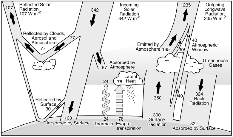
https://scienceofdoom.com/2010/07/17/the-amazing-case-of-back-radiation/
Dr. Strangelove,
I do account for the albedo effect in the calculation of Pi and its dependence on the cloud cover and other second order factors. What makes this somewhat confusing is that clouds, which are what converges the system to a steady state, affects both Pi and Po in roughly equal, but not exactly equal, proportions.