We publish this here, not to confirm that it is correct, but to stimulate the debate needed to determine whether or not it is correct or if it’s simply an exercise in curve fitting. ~ctm
George White, August 2017
Climate science is the most controversial science of the modern era. A reason why the controversy has been so persistent is that those who accept the IPCC as the arbiter of climate science fail to recognize that a controversy even exists. Their rationalization is that the IPCC’s conclusions are presented as the result of a scientific consensus, therefore, the threshold for overturning them is so high, it can’t be met, especially by anyone who’s peer reviewed work isn’t published in a main stream climate science journal. Their universal reaction when presented with contraindicative evidence is that there’s no way it can be true, therefore, it deserves no consideration and whoever brought it up can be ignored while the catch22 makes it almost impossible to get contraindicative evidence into any main stream journal.
This prejudice is not limited to those with a limited understanding of the science, but is widespread among those who think they understand and even quite prevalent among notable scientists in the field. Anyone who has ever engaged in communications with an individual who has accepted the consensus conclusions has likely observed this bias, often accompanied with demeaning language presented with extreme self righteous indignation that you would dare question the ‘settled science’ of the consensus.
The Fix
Correcting broken science that’s been settled by a consensus is made more difficult by its support from recursive logic where the errors justify themselves by defining what the consensus believes. The best way forward is to establish a new consensus. This means not just falsifying beliefs that support the status quo, but more importantly, replacing those beliefs with something more definitively settled.
Since politics has taken sides, climate science has become driven by the rules of politics rather than the rules of science. Taking a page from how a political consensus arises, the two sides must first understand and acknowledge what they have in common before they can address where they differ.
Alarmists and deniers alike believe that CO2 is a greenhouse gas, that GHG gases contribute to making the surface warmer than it would be otherwise, that man is putting CO2 into the atmosphere and that the climate changes. The denier label used by alarmists applies to anyone who doesn’t accept everything the consensus believes with the implication being that truths supported by real science are also being denied. Surely, if one believes that CO2 isn’t a greenhouse gas, that man isn’t putting CO2 into the atmosphere, that GHG’s don’t contribute to surface warmth, that the climate isn’t changing or that the laws of physics don’t apply, they would be in denial, but few skeptics are that uninformed.
Most skeptics would agree that if there was significant anthropogenic warming, we should take steps to prepare for any consequences. This means applying rational risk management, where all influences of increased CO2 and a warming climate must be considered. Increased atmospheric CO2 means more raw materials for photosynthesis, which at the base of the food chain is the sustaining foundation for nearly all life on Earth. Greenhouse operators routinely increase CO2 concentrations to be much higher than ambient because it’s good for the plants and does no harm to people. Warmer temperatures also have benefits. If you ask anyone who’s not a winter sports enthusiast what their favorite season is, it will probably not be winter. If you have sufficient food and water, you can survive indefinitely in the warmest outdoor temperatures found on the planet. This isn’t true in the coldest places where at a minimum you also need clothes, fire, fuel and shelter.
While the differences between sides seems irreconcilable, there’s only one factor they disagree about and this is the basis for all other differences. While this disagreement is still insurmountable, narrowing the scope makes it easier to address. The controversy is about the size of the incremental effect atmospheric CO2 has on the surface temperature which is a function of the size of the incremental effect solar energy has. This parameter is referred to as the climate sensitivity factor. What makes it so controversial is that the consensus accepts a sensitivity presumed by the IPCC, while the possible range theorized, calculated and measured by skeptics has little to no overlap with the range accepted by the consensus. The differences are so large that only one side can be right and the other must be irreconcilably wrong, which makes compromise impossible, perpetuating the controversy.
The IPCC’s sensitivity has never been validated by first principles physics or direct measurements. It’s most widely touted support comes from models, but it seems that as they add degrees of freedom to curve fit the past, the predictions of the future get alarmingly worse. Its support from measurements comes from extrapolating trends arising from manipulated data where the adjustments are poorly documented and the fudge factors always push results in one direction. This introduces even less certain unknowns, which are how much of the trend is a component of natural variability, how much is due to adjustments and how much is due to CO2. This seems counterproductive since the climate sensitivity should be relatively easy to predict using the settled laws of physics and even easier to measure with satellite observations, so what’s the point in the obfuscation by introducing unnecessary levels of indirection, additional unknowns and imaginary complexity?
Quantifying the Relationships
To quantify the sensitivity, we must start from a baseline that everyone can agree upon. This would be the analysis for a body like the Moon which has no atmosphere and that can be trivially modeled as an ideal black body. While not rocket science, an analysis similar to this was done prior to exploring the Moon in order to establish the required operational limits for lunar hardware. The Moon is a good place to start since it receives the same amount of solar energy as Earth and its inorganic composition is the same. Unless the Moon’s degenerate climate system can be accurately modeled, there’s no chance that a more complex system like the Earth can ever be understood.
To derive the sensitivity of the Moon, construct a behavioral model by formalizing the requirements of Conservation Of Energy as equation 1).
1) Pi(t) = Po(t) + ∂E(t)/∂t
Consider the virtual surface of matter in equilibrium with the Sun, which for the Moon is the same as its solid surface. Pi(t) is the instantaneous solar power absorbed by this surface, Po(t) is the instantaneous power emitted by it and E(t) is the solar energy stored by it. If Po(t) is instantaneously greater than Pi(t), ∂E(t)/∂t is negative and E(t) decreases until Po(t) becomes equal to Pi(t). If Po(t) is less than Pi(t), ∂E(t)/∂t is positive and E(t) increases until again Po(t) is equal to Pi(t). This equation quantifies more than just an ideal black body. COE dictates that it must be satisfied by the macroscopic behavior of any thermodynamic system that lacks an internal source of power, since changes in E(t) affect Po(t) enough to offset ∂E(t)/∂t. What differs between modeled systems is the nature of the matter in equilibrium with its energy source, the complexity of E(t) and the specific relationship between E(t) and Po(t). An astute observer will recognize that if an amount of time, τ, is defined such that all of E is emitted at the rate Po, the result becomes Pi = E/τ + ∂E/∂t which is the same form as the differential equation describing the charging and discharging of a capacitor which is another COE derived model of a physical system whose solutions are very well known where τ is the RC time constant.
For an ideal black body like the Moon, E(t) is the net solar energy stored by the top layer of its surface. From this, we can establish the precise relationship between E(t) and Po(t) by first establishing the relationship between the temperature, T(t) and E(t) as shown by equation 2).
2) T(t) = κE(t)
The temperature of matter and the energy stored by it are linearly dependent on each other through a proportionality constant, κ, which is a function of the heat capacity and equivalent mass of the matter in direct equilibrium with the Sun. Next, equation 3) quantifies the relationship between T(t) and Po(t).
3) Po(t) = εσT(t)4
This is just the Stefan-Boltzmann Law where σ is the Stefan Boltzmann constant and equal to about 5.67E-8 W/m2 per T4, and for the Moon, the emissivity of the surface, ε, is approximately equal to 1.
Pi(t) can be expressed as a function of Solar energy, Psun(t), and the albedo, α, as shown in equation 4).
4) Pi(t) = Psun(t)(1 – α)
Going forward, all of the variables will be considered implicit functions of time. The model now has 4 equations and 7 variables, Psun, Pi, Po, T, α, κ and ε. Psun is known for all points in time and space across the Moon’s surface. The albedo α and heat capacity κ are mostly constant across the surface and ε is almost exactly 1. To the extent that Psun, α, κ and ε are known, we can reduce the problem to 4 equations and 4 unknowns, Pi, T, Po and E, whose time varying values can be calculated for any point on the surface by solving a simple differential equation applied to an equal area gridded representation whose accuracy is limited only by the accuracy of α, κ and ε per cell. Any model that conforms to equations 1) through 4) will be referred to as a Physical Model.
Quantifying the Sensitivity
Starting from a Physical Model, the Moon’s sensitivity can be easily calculated. The ∂E/∂t term is what the IPCC calls ‘forcing’ which is the instantaneous difference between Pi and Po at TOA and/or TOT. For the Moon, TOT and TOA are coincident with the solid surface defining the virtual surface in direct equilibrium with the Sun. The IPCC defines forcing like this so that an increase in Pi owing to a decrease in albedo or increase in solar output can be made equivalent to a decrease in Po from a decrease in power passing through the transparent spectrum of the atmospheric that would arise from increased GHG concentrations. This definition is ambiguous since Pi is independent of E, while Po is highly dependent on E, thus a change in Pi is not equivalent to a the same change in Po since both change E, while only Po changes in response to changes in E which initiates further changes E and Po. The only proper characterization of forcing is a change in Pi and this is what will be used here.
While ∂E/∂t is the instantaneous difference between Pi and Po and conforms to the IPCC definition of forcing, the IPCC representation of the sensitivity assumes that ∂T/∂t is linearly proportional to ∂E/∂t, or at least approximately so. This is incorrect because of the T4 relationship between T and Po. The approximately linear assumption is valid over a small temperature range around average, but is definitely not valid over the range of all possible temperatures.
To calculate the Long Term Equilibrium sensitivity, we must consider that in the steady state, the temporal average of Pi is equal to the temporal average of Po, thus the integral over time of dE/dt will be zero. Given that in LTE, Pi is equal to Po, and the Moon certainly is in an LTE steady state, we can write the LTE balance equation as,
5) Pi = Po = εσT4
To calculate the LTE sensitivity, simply differentiate and invert the above equation which gives us,
6) ∂T/∂Pi = ∂T/∂Po = 1/(4εσT3)
This derivation does make an assumption, which is that ∂T/∂Pi = ∂T/∂Po since we’re really calculating ∂T/∂Po. For the Moon this is true, but for a planet with an semi-transparent atmosphere between the energy source and the surface in equilibrium with it, they aren’t for the same reason that the IPCC’s metric of forcing is ambiguous. None the less, what makes them different can be quantified and the quantification can be tested. But for the Moon, which will serve as the baseline, it doesn’t matter.
Define the average temperature of the Moon as the equivalent temperature of a black body where each square meter of surface is emitting the same amount of power such that when summed across all square meters, it adds up to the actual emissions. Normalizing to an average rate per m2 is a meaningful metric since all Joules are equivalent and the average of incoming and outgoing rates of Joules is meaningful for quantifying the effects one has on the other, moreover; a rate of energy per m2 can be trivially interchanged with an equivalent temperature. This same kind of average is widely applied to the Earth’s surface when calculating its average temperature from satellite data where the resulting surface emissions are converted to an equivalent temperature using the Stefan-Boltzmann Law.
If the average temperature of the Moon was 255K, equation 6) tells us that ∂T/∂Pi is about 0.3C per W/m2. If it was the 288K like the Earth, the sensitivity would be about 0.18C per W/m2. Notice that owing to the 1/T3 dependence of the sensitivity on temperature, as the temperature increases, the sensitivity decreases at an exponential rate. The average albedo of the Moon is about 0.12 leading to an average Pi and Po of about 300 W/m2 corresponding to an equivalent average temperature of about 270K and an average sensitivity of about 0.22 C per W/m2.
As far as the Moon is concerned, this analysis is based on nothing but first principles physics and the undeniable, deterministic average sensitivity that results is about 0.22C per W/m2. This is based on indisputable science, moreover; the predictions of Lunar temperatures using models like this have been well validated by measurements.
The 270K average temperature of the Moon would be the Earth’s average temperature if there were no GHG’s since this also means no liquid water, ice or clouds resulting in an Earth albedo of 0.12 just like the Moon. This contradicts the often repeated claim that GHG’s increase the temperature of Earth from 255K to 288K, or about 33C, where 255K is the equivalent temperature of the 240 W/m2 average power arriving at the planet after reflection. This is only half the story and it’s equally important to understand that water also cools the planet by about 15K owing to the albedo of clouds and ice which can’t be separated from the warming effect of water vapor making the net warming of the Earth from all effects about 18C and not 33C. Water vapor accounts for about 2/3 of the 33 degrees of warming leaving about 11C arising from all other GHG’s and clouds. The other GHG’s have no corresponding cooling effect, thus the net warming due to water is about 7C (33*2/3 – 15) while the net warming from all other sources combined is about 11C, where only a fraction of this arises from from CO2 alone.
Making It More Complex
Differences arise as the system gets more complex. At a level of complexity representative of the Earth’s climate system, the consensus asserts that the sensitivity increases all the way up to 0.8C per W/m2, which is nearly 4 times the sensitivity of a comparable system without GHG’s. Skeptics maintain that the sensitivity isn’t changing by anywhere near that much and remains close to where it started from without GHG’s and if anything, net negative feedback might make it even smaller.
Lets consider the complexity in an incremental manner, starting with the length of the day. For longer period rotations, the same point on the surface is exposed to the heat of the Sun and the cold of deep space for much longer periods of time. As the rotational speed increases, the difference between the minimum and maximum temperature decreases, but given the same amount of total incident power, the average emissions and equivalent average temperature will remain exactly the same. At real slow rotation rates, the dark side can emit all of the energy it ever absorbed from the Sun and the surface emissions will approach those corresponding to it’s internal temperature which does affect the result.
The sensitivity we care about is relevant to how the LTE averages change. The average emissions and corresponding average temperature are locked to an invariant amount of incident solar energy while the rotation rate has only a small effect on the average sensitivity related to the T-3 relationship between temperature and the sensitivity. Longer days and nights mean that local sensitivities will span a wider range owing to a wider temperature range. Since higher temperatures require a larger portion of the total energy budget, as the rotation rate slows, the average sensitivity decreases. To normalize this to Earth, consider a Moon with a 24 hour day where this effect is relatively small.
The next complication is to add an atmosphere. Start with an Earth like atmosphere of N2, O2, and Ar except without water or other GHG’s. On the Moon, gravity is less, so it will take more atmosphere to achieve Earth like atmospheric pressures. To normalize this, consider a Moon the size of the Earth and with Earth like gravity.
The net effect of an atmosphere devoid of GHG’s and clouds will also reduce the difference between high and low extremes, but not by much since dry air can’t hold and transfer much heat, nor will there be much of a difference between ∂T/∂Pi and ∂T/∂Po. Since O2, N2 and Ar are mostly transparent to both incoming visible light and outgoing LWIR radiation, this atmosphere has little impact on the temperature, the energy balance or the sensitivity of the surface temperature to forcing.
At this point, we have a Physical Model representative of an Earth like planet with an Earth like atmosphere, except that it contains no GHG’s, clouds, liquid or solid water, the average temperature is 270K and the average sensitivity is 0.22 W/m2. It’s safe to say that up until this point in the analysis, the Physical Model is based on nothing but well settled physics. There’s still an ocean and a small percentage of the atmosphere to account for, comprised mostly of water and trace gases like CO2, CH4 and O3.
The Fun Starts Here
The consensus contends that the Earth’s climate system is far too complex to be represented with something as deterministic as a Physical Model, even as this model works perfectly well for an Earth like planet missing only water a few trace gases. They arm wave complexities like GHG’s, clouds, coupling between the land, oceans and atmosphere, model predictions, latent heat, thermals, non linearities, chaos, feedback and interactions between these factors as contributing to making the climate too complex to model in such a trivial way, moreover; what about Venus? Each of these issues will be examined by itself to see what effects it might have on the surface temperature, planet emissions and the sensitivity as quantified by the Physical Model, including how this model explains Venus.
Greenhouse Gases
When GHG’s other than water vapor are added to the Physical Model, the effect on the surface temperature can be readily quantified. If some fraction of the energy emitted by the surface is captured by GHG molecules, some fraction of what was absorbed by those molecules is ultimately returned to the surface making it warmer while the remaining fraction is ultimately emitted into space manifesting the energy balance. This is relatively easy to add to the model equations as a decrease in the effective emissivity of a surface at some temperature relative to the emissions of a planet. If Ps is the surface emissions corresponding to T, Fa is the fraction of Ps that’s captured by GHG’s and Fr is the fraction of the captured power returned to the surface, we can express this in equations 7) and 8).
7) Ps = εxσT4
8) Po = (1 – Fa)Ps + FaPs(1 – Fr)
The first term in equation 8) is the power passing though the atmosphere that’s not intercepted by GHG’s and the second term is the fraction of what was captured and ultimately emitted into space. Solving equation 8) for Po/Ps, we get equation 9),
9) Po/Ps = 1 – FaFr
Now, we can combine with equation 9) with equation 7) to rewrite equation 3) as equation 3a).
3a) Po = (1 – FaFr)εxσT4
Here, εx is the emissivity of the surface itself, which like the surface of the Moon without GHG’s is also approximately 1, where (1 – FaFr) is the effective emissivity contributed by the semi-transparent atmosphere. This can be double checked by calculating Psi, which is the power incident to the surface and by recognizing that Psi – Ps is equal to ∂E/∂t and Pi – Po.
10) Psi = Pi + PsFaFr
11) Psi – Ps = Pi – Po
Solving 11) for Psi and substituting into 10), we get equation 12), solving for Po results in 13) which after substituting 7) for Ps is yet another way to arrive at equation 3a).
12) Ps – Po = PsFaFr
13) Po = (1 – FaFr)Ps
The result is that adding GHG’s modifies the effective emissivity of the planet from 1 for an ideal black body surface to a smaller value as the atmosphere absorbs some fraction of surface emissions making the planets emissions, relative to its surface temperature, appear gray from space. The effective emissivity of this gray body emitter, ε’, is given exactly by equation 3a) as ε’ = (1 – FaFr)εx.
Clouds
Clouds are the most enigmatic of the complications, but none the less can easily fit within the Physical Model. The way to model clouds is to characterize them by the fraction of surface covered by them and then apply the Physical Model with values of α, κ and ε specific to average clear and average cloudy skies and then weighting the results based on the specific proportions of each.
Consider the Pi term, where if ρ is the fraction of the surface covered by clouds, αc is the average albedo of cloudy skies and αs is the average albedo of clear skies, α can be calculated as equation 14).
14) α = ραc + (1 – ρ)αs
Now, consider the Po term, which can be similarly calculated as equation 15) where Ps and Pc are the emissions of the surface and clouds at their average temperatures, εs is the equivalent emissivity characterizing the clear atmosphere and εc is the equivalent emissivity characterizing clouds.
15) Po = ρεsεcPc + ρ(1 – εc)εsPs + (1 – ρ)εsPs
The first term is the power emitted by clouds, the second term is the surface power passing through clouds and the last term is the power emitted by the surface and passing through the clear sky. GHG’s can be accounted for by identifying the value of εs corresponding to the average absorption characteristics between the surface and space and between clouds and space. By considering Pc as some fraction of Ps and calling this Fx, equation 15) can be rearranged to calculate Po/Ps which is the same as the ε’ derived from equation 3a). The result is equation 16).
16) ε’ = Po/Ps = ρεs εcFx + ρεs (1 – εc) + (1 – ρ)εs
The variables εc, Fx and ρ can all be extracted from the ISCCP cloud data, as can αc and αs., moreover; the data supports a very linear relationship between Pc and Ps. The average value of ρ is 0.66, the average value of αc is 0.37 and αs is 0.16 resulting in a value for α of about 0.30 which is exactly equal to the accepted value. The average value of εc is about 0.72 and Fx is measured to be about 0.68. Considering εs to be 1, the effective ε’ is calculated to be about 0.85.
From line by line simulations of a standard atmosphere, the fraction of surface and cloud emissions absorbed by GHG’s, Fa, is about 0.58, the value of Fr as constrained by geometry is 0.5 and is measured to be about 0.51. From equation 13), the equivalent εs becomes 0.71. The new ε’ becomes 0.85 * 0.70 = 0.60 which is well within the margin of error for the expected value of Po/Ps which is 240/395 = 0.61 and even closer to the measured value from the ISCCP data of 238/396 = 0.60. When the same analysis is performed one hemisphere at a time, or even on individual slices of latitude, the predicted ratios of Po/Ps match the measurements once the net transfer of energy from the equator to the poles and between hemispheres is properly accounted for.
At this point, we have a Physical Model that accounts for GHG’s and clouds which accurately predicts the ratio between the BB surface emissions at its average temperature and predicts the average emissions of the planet spanning the entire range of temperatures found on the surface.
The applicability of the Physical Model to the Earth’s climate system is a hypothesis derived from first principles, which still must be tested. The first test predicting the ratio of the planets emissions to surface emissions got the right answer, but this is a simple test and while questioning the method is to deny physical laws, surely some will question the coefficients that led to this result. While the coefficients aren’t constant, they do vary around a mean and its the mean value that’s relevant to the LTE sensitivity. A more powerful testable prediction is that of the planets emissions as a function of surface temperature. The LTE relationship predicted by equation 3) is that if Po are the emissions of the planet and T is the surface temperature, the relationship between them is that of a gray body whose temperature is T and whose emissivity is ε’ and which is calculated to be about 0.61. The results of this test will be presented a little later along with justification for the coefficients used for the first test.
Complex Coupling
In the context of equation 1), complex couplings are modeled as individual storage pools of E that exchange energy among themselves. We’re only concerned about the LTE sensitivity, so by definition, the net exchange of energy among all pools contributing to the temperature must be zero. Otherwise, parts of the system will either heat up or cool down without bound. LTE is defined when the average ∂E/∂t is zero, thus the rate of change for the sum of its components must also be zero.
Not all pools of E necessarily contribute to the surface temperature. For example, some amount of E is consumed by photosynthesis and more is consumed to perform the work of weather. If we quantify E as two pools, one storing the energy that contributes to the surface temperature Es, and the energy stored in all other pools as Eo, we can rewrite equations 1) and 2) as,
1) Pi = Po + ∂Es/∂t + ∂Eo/∂t
1a) ∂E/∂t = ∂Es/∂t + ∂Eo/∂t
2a) T = κ(Es – Eo)
If Eo is a small percentage of Es, an equivalent κ’ can be calculated such that κ’E = κ(Es – Eo) and the Physical Model is still representative of the system as a whole and the value of κ’ will not deviate much from its theoretical value. Measurements from the ISCCP data suggest an average of about 1.8 +/- 0.5 W/m2 of the 240 W/m2 of the average incident solar energy is not contributing to heating the planet nor must it be emitted for the planet to be in a thermodynamic steady state.
Thus far, GHG’s, clouds and the coupling between the surface, oceans and atmosphere can all be accommodated with the Physical Model, by simply adjusting α, κ and ε. There can be no question that the Physical Model is capable of modeling the Earth’s climate and that per equation 6), the upper bound on the sensitivity is less than the 0.4C per W/m2 lower bound suggested by the IPCC. The rest of this discussion will address why the issues with this model are invalid, demonstrate tests whose results support predictions of the Physical Model and show other tests that falsify a high sensitivity.
Models
The results of climate models are frequently cited as supporting an ‘emergent’ high sensitivity, however; these models tend to include errors and assumptions that favor a high sensitivity. Many even dial in a presumed sensitivity indirectly. The underlying issue is that the GCM’s used for climate modeling have a very large number of coefficients whose values are unknown, so they are set based on ‘educated’ guesses and it’s this that leads to bias as objectivity is replaced with subjectivity.
In order to match the past, simulated annealing like algorithms are applied to vary these coefficients around their expected mean until the past is best matched, which if there are any errors in the presumed mean values or there are any fundamental algorithmic flaws, the effects of these errors accumulate making both predictions of the future and the further past worse. This modeling failure is clearly demonstrated by the physics defying predictions so commonly made by these models.
Consider a sine wave with a gradually increasing period. If the model used to represent it is a fixed period sine wave and the period of the model is matched to the average period of a few observed cycles, the model will deviate from what’s being modeled both before and after the range over which the model was calibrated. If the measurements span less than a full period, both a long period sine wave and a linear trend can fit the data, but when looking for a linear trend, the long period sine wave becomes invisible. Consider seasonal variability, which is nearly perfectly sinusoidal. If you measure the average linear trend from June to July and extrapolate, the model will definitely fail in the past and the future and the further out in time you go, the worse it will get. Notice that only sinusoidal and exponential functions of E work as solutions for equation 1), since only sinusoids and exponentials have a derivative whose form is the same as itself, given that Po is a function of E. Note that the theoretical and actual variability in Pi can be expressed as the sum of sinusoids and exponentials and that this leads to the linear property of superposition when behavior is modeled in the energy in, energy out domain, rather than in the energy in, temperature out domain preferred by the IPCC.
The way to make GCM’s more accurate is to insure that the macroscopic behavior of the system being modeled conforms to the constraints of the Physical Model. Clearly this is not being done, otherwise the modeled sensitivity would be closer to 0.22 C per W/m2 and no where near the 0.8C per W/m2 presumed by the consensus and supported by the erroneous models.
Non Radiant Energy
Adding non radiant energy transports to the mix adds yet another level of obfuscation. This arises from Trenberth’s energy balance which includes latent heat and thermals transporting energy into the atmosphere along with the 390 W/m2 of radiant energy arising from an ideal black body surface at 288K. Trenberth returns the non radiant energy to the surface as part of the ‘back radiation’ term, but its inclusion gets in the way of understanding how the energy balance relates to the sensitivity, especially since most of the return of this energy is not in the form of radiation, but in the form of air and water returning that energy back to the surface.
The reason is that neither latent heat, thermals or any other energy transported by matter into the atmosphere has any effect on the surface temperature, input flux or emissions of the planet, beyond the effect they are already having on these variables and whatever effects they have is bundled into the equivalent values of α, κ and ε. The controversy is about the sensitivity, which is the relationship between changes in Pi and changes in T. The Physical Model ascribed with equivalent values of α, κ and ε dictates exactly what the sensitivity must be. Since Pi, Po and T are all measurable values, validating that the net results of these non radiative transports are already accounted for by the relative relationships of measurable variables and that these relationships conform to the Physical Model is very testable and whose results are very repeatable.
Chaos and Non Linearities
Chaos and non linearities are a common complication used to dismiss the requirement that the macroscopic climate system behavior must obey the macroscopic laws of physics. Chaos is primarily an attribute of the path the climate system takes from one equilibrium state to another and is also called weather, which of course, is not the climate. Relative to the LTE response of the system and its corresponding LTE sensitivity, chaos averages out since the new equilibrium state itself is invariant and driven by the incident energy and its conservation. Even quasi-stable states like those associated with ENSO cycles and other natural variability averages out relative to the LTE state.
Chaos may result in over shooting the desired equilibrium, in which case it will eventually migrate back to where it wants to be, but what’s more likely, is that the system never reaches its new steady state equilibrium because some factor will change what that new steady state will be. Consider seasonal variability, where the days start getting shorter or longer before the surface reaches the maximum or minimum temperature it could achieve if the day length was consistently long or short.
Non linearities are another of these red herrings and the most significant non linearity in the system as modeled by the IPCC is the relationship between emissions and temperature. By keeping the analysis in the energy domain and converting to equivalent temperatures at the end, the non linearities all but disappear.
Feedback
Large positive feedback is used to justify how 1 W/m2 of forcing can be amplified into the 4.3 W/m2 of surface emissions required in order to sustain a surface temperature 0.8C higher than the current average of 288K. This is ridiculous considering that the 240 W/m2 of accumulated forcing (Pi) currently results in 390 W/m2 of radiant emissions from the surface (Ps) and that each W/m2 of input results in only 1.6 W/m2 of surface emissions. This means that the last W/m2 of forcing from the Sun resulted in about 1.6 W/m2 of surface emissions, the idea that the next one would result in 4.3 W/m2 is so absurd it defies all possible logic. This represents such an obviously fatal flaw in consensus climate science that either the claimed sensitivity was never subject to peer review or the veracity of climate science peer review is nil, either of which deprecates the entire body of climate science publishing.
The feedback related errors were first made by Hansen, reinforced by Schlesinger and have been cast in stone since AR1 and more recently, they’ve been echoed by Roe. Bode developed an analysis technique for linear, feedback amplifiers and this analysis was improperly applied to quantify climate system feedback. Bode’s model has two non negotiable preconditions that were not met by the application of his analysis to the climate. These are specified in the first couple of paragraphs in the book referenced by both Hansen and Schlesinger as the theoretical foundation for climate feedback. First is the assumption of strict linearity. This means that if the input changes by 1 and the output changes by 2, then, if the input changes by 2, the output must change by 4. By using a delta Pi as the input to the model and a delta T as the output, this linearity constraint was violated since power and temperature are not linearly related, but power is related to T4. Second is the requirement for an implicit source of Joules to power the gain. This can’t be the Sun, as solar energy is already accounted for as the forcing input to the model and you can’t count it twice.
To grasp the implications of nonlinearity, consider an audio amplifier with a gain of 100. If 1 V goes in and 100 V comes out before the amplifier starts to clip, increasing the input to 2V will not change the output value and the gain, which was 100 for inputs from 0V to 1V is reduced to 50 at 2V of input. Bode’s analysis requires the gain, which climate science calls the sensitivity, to be constant and independent of the input forcing. Once an amplifier goes non linear and starts to clip, Bode’s analysis no longer applies.
Bode defines forcing as the stimulus and defines sensitivity as the change in the dimensionless gain consequential to the change in some other parameter and is also a dimensionless ratio. What climate science calls forcing is an over generalization of the concept and what they call sensitivity is actually the incremental gain, moreover; they’ve voided the ability to use Bode’s analysis by choosing a non linear metric of gain. For the linear systems modeled by Bode, the incremental gain is always equal to the absolute gain as this is the basic requirement that defines linearity. The consensus makes the false claim that the incremental gain can be many times larger than the absolute gain, which is a non sequitur relative to the analysis used. Furthermore, given the T-3 dependence of the sensitivity on the temperature, the sensitivity quantified as a temperature change per W/m2 of forcing must decrease as T increases, while the consensus quantification of the sensitivity requires the exact opposite.
At the measured value of 1.6 W/m2 of surface emissions per W/m2 of accumulated solar forcing, the extra 0.6 W/m2 above and beyond the initial W/m2 of forcing is all that can be attributed to what climate science refers to as feedback. The hypothesis of a high sensitivity requires 3.3 W/m2 of feedback to arise from only 1 W/m2 of forcing. This is 330% of the forcing and any system whose positive feedback exceeds 100% of the input will be unconditionally unstable and the climate system is certainly stable and always recovers after catastrophic natural events that can do far more damage to the Earth and its ecosystems then man could ever do in millions of years of trying. Even the lower limit claimed by the IPCC of 0.4C per W/m2 requires more than 100% positive feedback, falsifying the entire range they assert.
An irony is that consensus climate science relies on an oversimplified feedback model that makes explicit assumptions that don’t apply to the climate system in order to support the hypothesis of a high sensitivity arising from large positive feedback, yet their biggest complaint about the applicability of the Physical Model is that the climate is too complicated to be represented with such a simple and undeniably deterministic model.
Venus
Venus is something else that climate alarmists like to bring up. However; if you consider Venus in the context of the Physical Model, the proper surface in direct equilibrium with the Sun is not the solid surface of the planet, but a virtual surface high up in its clouds. Unlike Earth, where the lapse rate is negative from the surface in equilibrium with the Sun and up into the atmosphere, the Venusian lapse rate is positive from its surface in equilibrium with the Sun down to the solid surface below. Even if the Venusian atmosphere was 90 ATM of N2, the surface would still be about as hot as it is now.
Venus is a case of runaway clouds and not runaway GHG’s as often claimed. The thermodynamics of Earth’s clouds are tightly coupled to that of its surface through evaporation and precipitation, thus cloud temperatures are a direct function of the surface temperature below and not the Sun. While the water in clouds does absorb some solar energy, owing to the tight coupling between clouds and the oceans, the LTE effect is the same as if the oceans had absorbed that energy directly. This isn’t the case for Venus, where the thermodynamics of its clouds are independent from that of its surface enabling clouds to arrive at a steady state with incoming energy by themselves.
Even for Earth, the surface in direct equilibrium with the Sun is not the solid surface, as it is for the Moon, but is a virtual surface comprised of the top of the oceans and the bits of land that poke through. Most of the solid surface is beneath the oceans and its nearly 0C temperature is a function of the temperature/density profile of the ocean above. The dense CO2 atmosphere of Venus, whose mass is comparable to the mass of Earth’s oceans, acts more like Earth’s oceans than it does Earth’s atmosphere thus Venusian cloud tops above a CO2 ocean is a good analogy for the surface of Earth and will be at about the same average temperature and atmospheric pressure.
Testing Predictions
The Physical Model makes predictions about how Pi, Po and the surface temperature will behave relative to each other. The first test was a prediction of the ratio between surface emissions and planet emissions based on measurable physical parameters and this calculation was nearly exact. The values of αc, αs, ρ, and εc in equations 14) and 16) were extracted as the average values reported or derived from the ISCCP cloud data set provided by GISS while εs arose from line by line simulations.
Figures 1, 2, 3 and 4 illustrate the origins of αc, αs, ρ, and εc, where the dotted line in each plot represents the measured LTE average value for that parameter. Those values were rounded to 2 significant digits for the purpose of checking the predictions of equations 14) and 16). Clicking
on a figure should bring up a full resolution version.


The absolute accuracy of ISCCP surface temperatures suffers from a 2001 change to a new generation of polar orbiters combined with discontinuous polar orbiter coverage which the algorithms depended on for consistent cross satellite calibration. This can be seen more dramatically in Figure 5, which is a plot of the global monthly average surface temperature derived from the gridded temperatures reported in the ISSCP. While this makes the data useless for establishing trends, it doesn’t materially affect the use of this data for establishing the average coefficients related to the sensitivity.


Figure 5 demonstrates something even more interesting, which is that the two hemispheres don’t exactly cancel and the peak to peak variability in the global monthly average is about 5C. The Northern hemisphere has significantly more seasonal p-p temperature variability than the Southern hemisphere owing to a larger fraction of land resulting in a global sum whose minimum and maximum are 180 degrees out of phase of what you would expect from the seasonal position of perihelion. To the extent that the consensus assumes the effects of perihelion average out across the planet, the 5C p-p seasonal variability in the planets average temperature represents the minimum amount of natural variability to expect given the same amount of incident energy. In about 10K years when perihelion is aligned with the Northern hemisphere summer, the p-p differences between hemispheres will become much larger which is a likely trigger for the next ice age. The asymmetric response of the hemispheres is something that consensus climate science has not wrapped its collective heads around, largely because the anomaly analysis they depend on smooths out seasonal variability obfuscating the importance of understanding how and why this variability arises, how quickly the planet responds to seasonal forcing and how the asymmetry contributes to the ebb and flow of ice ages.
While Pi is trivially calculated as reflectance applied to solar energy, both of which are relatively accurately known, Po is trickier to arrive at. Satellites only measure LWIR emissions in 1 or 2 narrow bands in the transparent regions of the emission spectrum and in an even narrower band whose magnitude indicates how much water vapor absorption is taking place. These narrow band emissions are converted to a surface temperature by applying a radiative model to a varying temperature until the emissions leaving the radiative model in the bands measured by the satellite are matched and then the results are aligned to surface measurements. Equation 15) was used to calculate Po which was based on reported surface temperatures, cloud temperatures and cloud emissivity applied to a reverse engineered radiative model to determine how much power leaves the top of the atmosphere across all bands. This is done for both cloudy and clear skies across each equal area grid cell and the total emissions are a sum weighted by the fraction of clouds modified by the clouds emissivity. To cross check this calculation, ∂E(t)/∂t can be calculated as the difference between Pi and the derived Po. If the long term average of this is close to zero, then COE is not violated by the calculated Po. Figure 6 shows this and indeed, the average ∂E(t)/∂t is approximately zero within the accuracy of the data. The 1.8 W/m2 difference could be a small data error, but seems to be the solar power that’s not actually heating the surface but powering photosynthesis and driving the weather and that need not be emitted for balance to arise. Note that ∂E/∂t per hemisphere is about 200 W/m^2 p-p and that the ratio between the global ∂E/∂t and the global ∂T/∂t infers a transient sensitivity of only about 0.12 C per W/m^2.
Figure 7 shows another way to validate the predictions as a scatter plot of the relative relationship between monthly averages of Pi and Po for constant latitude. Each little dot is the average for 1 month of data and the larger dots are the per slice averages across 3 decades of measurements. The magenta line represents Pi == Po. Where the two curves intersect defines the steady state which at 239 W/m2 is well within the margin of error of the accepted value. Note that the tilt in the measured relationships represents the net transfer of energy from tropical latitudes on the right to polar latitudes on the left.


The next test is of the prediction that the relationship between the average temperature of the surface and the planets emissions should correspond to a gray body emitter whose equivalent emissivity is about 0.61, which was the predicted and measured ratio between the planets emissions and that of the surface.
Figure 8 shows the relationship between the surface temperature and both Pi and Po, again for constant latitude slices of the planet. Constant latitude slices provide visibility to the sensitivity as the most significant difference between adjacent slices is Pi, where a change in Pi is forcing per the IPCC definition. The change in the surface temperature of adjacent slices divided by the change in Pi quantifies the sensitivity of that slice per the IPCC definition. The slope of the measured relationship around the steady state is the short line shown in green. The larger green line is a curve of the Stefan-Boltzmann Law predicting the complete relationship between the temperature and emissions based on the measured and calculated equivalent emissivity of 0.61. The monthly average relationship between Po and the surface temperature is measured to be almost exactly what was predicted by the Physical Model. The magenta line is the prediction of the relationship between Pi and the surface temperature based on the requirement that the surface is approximately an ideal black body emitter and again, the prediction is matched by the data almost exactly.
For reference, Figure 9 shows how little the effective emissivity, ε’ varies on a monthly basis with a max deviation from nominal of only about +/- 3%. Figure 10 shows how the fraction of the power absorbed by the atmosphere and returned to the surface also varies in a relatively small range around 0.51. In fact, the monthly averages for all of the coefficients used to calculate the sensitivity with equation 16) vary over relatively narrow ranges.


The hypothesized high sensitivity also makes predictions. The stated nominal sensitivity is 0.8C per W/m2 of forcing and if the surface temperature increases by 0.8C from 288K to 288.8K, 390.1 W/m2 of surface emissions increases to 394.4 W/m2 for a 4.3 W/m2 increase that must arise from only 1 W/m2 of forcing. Since the data shows that 1 W/m2 of forcing from the Sun increases the surface emissions by only 1 W/m2, the extra 3.3 W/m2 required by the consensus has no identifiable origin thus falsifies the possibility of a sensitivity as high as claimed. The only possible origin is the presumed internal power supply that Hansen and Schlesinger incorrectly introduced to the quantification of climate feedback.
Joules are Joules and are interchangeable with each other. If the next W/m2 of forcing will increase the surface emissions by 4.3 W/m2, each of the accumulated 239 W/m2 of solar forcing must be increasing the surface emissions by the same amount. If the claimed sensitivity was true, the surface would be emitting 1028 W/m2 which corresponds to an average surface temperature of 367K which is about 94C and close to the boiling point of water. Clearly it’s not once again falsifying a high sensitivity.
Conclusion
Each of the many complexities cited to diffuse a simple analysis based on the immutable laws of physics has been shown to be equivalent to variability in the α, κ and ε coefficients quantifying the Physical Model. Another complaint is that the many complexities interact with each other. To the extent they do and each by itself is equivalent to changes in α, κ and ε, any interactions can be similarly represented as equivalent changes to α, κ and ε. It’s equally important to remember that unlike GCM’s, this model has no degrees of freedom to tweak its behavior, other than the values of α, κ and ε, all of which can be measured, and that no possible combination of coefficients within factors of 2 of the measured values will result in a sensitivity anywhere close to what’s claimed by the consensus. The only possible way for any Physical Model to support the high sensitivity claimed by the IPCC is to violate Conservation Of Energy and/or the Stefan-Boltzmann Law which is clearly impossible.
Predictions made by the Physical Model have been confirmed with repeatable measurements while the predictions arising from a high sensitivity consistently fail. In any other field of science, this is unambiguous proof that the model whose predictions are consistently confirmed is far closer to reality than a model whose predictions consistently fail, yet the ‘consensus’ only accepts the failing model. This is because the IPCC, which has become the arbiter of what is and what is not climate science, needs the broken model to supply its moral grounds for a massive redistribution of wealth under the guise of climate reparations. It’s an insult to all of science that the scientific method has been superseded by a demonstrably false narrative used to support an otherwise unsupportable agenda and this must not be allowed to continue.
Here’s a challenge to those who still accept the flawed science supporting the IPCC’s transparently repressive agenda. First, make a good faith effort to understand how the Physical Model is relevant, rather than just dismiss it out of hand. If you need more convincing after that, try to derive the sensitivity claimed by the IPCC using nothing but the laws of physics. Alternatively, try to falsify any prediction made by the Physical Model, again, relying only on the settled laws of physics. Another thing to try is to come up with a better explanation for the data, especially the measured relationships between Pi, Po and the surface temperature, all of which are repeatably deterministic and conform to the Physical Model. If you have access to a GCM, see if its outputs conform to the Physical Model and once you understand why they don’t, you will no doubt have uncovered serious errors in the GCM.
If the high sensitivity claimed by the IPCC can be falsified, it must be rejected. If the broadly testable Physical Model produces the measured results and can’t be falsified, it must be accepted. Falsifying a high sensitivity is definitive and unless and until something like the Physical Model is accepted by a new consensus, climate science will remain controversial since no amount of alarmist rhetoric can change the laws of physics or supplant the scientific method.
References
1) IPCC reports, definition of forcing, AR5, figure 8.1
AR5 Glossary, ‘climate sensitivity parameter’
2) Kevin E. Trenberth, John T. Fasullo, and Jeffrey Kiehl, 2009: Earth’s Global Energy Budget. Bull. Amer. Meteor. Soc., 90, 311–323. Trenberth
3) 2) Bode H, Network Analysis and Feedback Amplifier Design
assumption of external power supply and active gain, 31 section 3.2
gain equation, 32 equation 3-3
real definition of sensitivity, 52-57 (sensitivity of gain to component drift)
3a) effects of consuming input power, 56, section 4.10
impedance assumptions, 66-71, section 5.2 – 5.6
a passive circuit is always stable, 108
definition of input (forcing) 31
4) Jouzel, J., et al. 2007: EPICA Dome C Ice Core 800KYr Deuterium Data and Temperature Estimates.
5) ISCCP Cloud Data Products: Rossow, W.B., and Schiffer, R.A., 1999: Advances in Understanding Clouds from ISCCP. Bull. Amer. Meteor. Soc., 80, 2261-2288.
6) Hansen, J., A. Lacis, D. Rind, G. Russell, P. Stone, I. Fung, R. Ruedy, and J. Lerner, 1984: Climate sensitivity: Analysis of feedback mechanisms. In Climate Processes and Climate Sensitivity, AGU Geophysical Monograph 29, Maurice Ewing Vol. 5. J.E. Hansen, and T. Takahashi, Eds. American Geophysical Union, 130-163.
7) M. E. Schlesinger (ed.), Physically-Based Modeling and Simulations of Climate and Climatic Change – Part II, 653-735
8) Michael E. Schlesinger. Physically-based Modelling and Simulation of Climate and Climatic Change (NATO Advanced Study Institute on Physical-Based Modelling ed.). Springer. p. 627. ISBN 90-277-2789-9
9) Gerard Roe. Feedbacks Timescales and Seeing Red, Annual Review of Earth Planet Science 2009, 37:93-115
10) Stefan, J. (1879), “Über die Beziehung zwischen der Wärmestrahlung und der Temperatur” [On the relationship between heat radiation and temperature] (PDF), 79: 391–428
11) Boltzmann, L. (1884), “Ableitung des Stefan’schen Gesetzes, betreffend die Abhängigkeit der Wärmestrahlung von der Temperatur aus der electromagnetischen Lichttheorie” 258 (6): 291–294
Looks like my reply to ristvan got lost in the ether. It was criticism of him and GW.
The mean equatorial temp of the moon is 220K. The mean of the daytime temp is 340K. Even without the GHE and same albedo, the Earth’s mean T should be a lot more for the same mean T^4 because the heat spreads.
Treating the moon like a black body is not the problem other than a BB should conduct the heat quickly throughout. Each square metre ( to cm depth?) might be close to BB independent of the rest of the moon.
Then there is rotation. The dark side of the moon cools to only 120K in the first 12 h before reaching 93 K at the equator. If the Earth were rock like the moon and warmed up quickly during the day to a mean of 340K at the eq, its 24h mean would be 240K, 20K large than the moon at the eq.
@Dale Rainwater. Strangelove
So, you remove 30% of the heat, then you notice your calculation is flawed, because heat is missing. Instead of realizing that your calculations are the problem, you do the one thing that is not allowed: heat transfer from cold to hot. And still, you don’t even bother to think about the fact that you removed heat before starting the calculation.
Use correct geometry instead. (TSI/(4π/3)²)/2π, no need for fudge.
If you think DLR has been measured, you need to learn how a pyrgeometer works.
Are you a Dragon Slayer? Here’s a tutorial on why greenhouse effect does not violate 2nd law of thermodynamics
https://scienceofdoom.com/2010/10/07/amazing-things-we-find-in-textbooks-the-real-second-law-of-thermodynamics/
I also agree that the GHG effect does not violate the second law. Photons don’t care about the temperature of its destination is and will still add energy to it when absorbed.
I have been debating the deceiver running that crappy blog. I repeatedly asked him about the violations in gh-theory and heat gave no answers. It was easier for him to ban me.
Dragonslayer? Always the name-calling when debating the warming from dry ice. I have started to do the same. I call you the blanket-people. Because you always use explanations with blankets to describe how dry ice in cold air makes hot surfaces warmer. You don’t Sven know fundamental TD-principles, that a blanket prevents absorption in surrounding air. A blanket does the opposite of what a gh-gas does.
You should ask *snip* why he used optical calculations to find temperatures. We have models for heat transfer, they work. But they can’t produce “back-radiation”, they show how the cold fluid atmosphere cools the surface. Of course. Have you ever experienced how cold damp air and dry ice makes you warmer? Didn’t think so.
Then why do you expect that from the atmosphere?
The second law says that heat nerver transfer from cold to hot without work being done on the system. The ” net”-BS from *snip* nothing else than him trying to deceive.
*interesting that you complain of name calling and then engage in it yourself*
Actually it’s more basic than even that if the cold body wasn’t radiating you infer GOD properties on each object that they have to know who is hotter than who to know if they are allowed to radiate. The only way not to infer GOD properties on everything must radiate and then you just subtract to the two as per your article.
Try doing a delayed choice experiment between a hot and a cold body and see how the dragon slayers fair as they won’t know whether it’s emitting or not because I am not going to choose or not to expose the two objects until a long time after the emission is required to leave the hot source. They suddenly will find they need thermal emissions to be faster than the speed of light 🙂
That is why I can’t understand DragonSlayers all they have to search is delayed choice experiments on thermal emissions and it’s pretty obvious what they think is wrong.
“LdB
10 minuter
Actually it’s more basic than even that if the cold body wasn’t radiating you infer GOD properties on each object that they have to know who is hotter than who to know if they are allowed to radiate. The only way not to infer GOD properties on everything must radiate and then you just subtract to the two as per your article. ”
I do the opposite, I infer NO properties. The whole idea behind my approach is to make zero assumptions. I use a noninteracting cavity with spherical shells that obey Gauss law for gravity. Only known, proven and applied physics.
There is not a single experimental study or data that supports a claim that a cold fluid at low temperature, can increase the emissive power of the heat source heating it.
Prevost, a pioneer, came to the conclusion that the emission from a body depends on the internal state only.
Let me make something clear, there is no honest way for you to argue that the atmosphere is part of the surface internal state. But let me see you try.
What Prevost said has not been questioned, are you brave enough to try?
Why did everyone forget to read what basic physics say.
I just follow what proven physics say about energy and geometry, and ignore theories that use the coldest part of a system as a heat source. Someday the greenhouse theory will be regarded as more stupid than flat-earth delusions.
But your idea doesn’t work as I said it fails the most basic tests.
At the very least your crazy physics stops radio signals working because you deny electromagnetic waves can be emit and received energy to the same source at different frequencies.
So you make zero assumptions but half of physics we use everyday drops dead in the water?????
Great physics idea .. love it and you just want to hand wave at it and expect me to not think you guys are are all crazy.
I don’t deny anything. You are the one maning assumptions about frequencies. I rely on proven and applied models that work. They clearly say that your explanation with back-radiation is irrelevant. The s-b law has not been falsified, so why do you question it?
Robert,
“Then there is rotation.”
Explain how the rotation affects the AVERAGE emissions of the Moon which must be equal to the average incident energy independent of the rate of rotation? You seem to be considering linear averages of temperature and not the proper average of emissions which in the end are converted to an EQUIVALENT average temperature. If Pi is X, Po must also be X, independent of the rotation rate and the average temperature is calculated by using SB to convert X to a temperature.
“Explain how the rotation affects the AVERAGE emissions of the Moon which must be equal to the average incident energy independent of the rate of rotation? ”
At night, the moon cools from 150K to 93 K over two weeks. Just a back of envelope assuming a 24 h day for the moon that it would only cool to 120-130 K you get a 20 K higher mean at the equator. It comes from the moon not cooling to close to 0 at night.
Robert,
Your explanation isn’t answering my question.
So what is happening to the difference between the energy arriving at the Moon and the energy emitted by it? If the average temperature calculated as the equivalent temperature of average emissions is different then the equivalent temperature of the incident radiation, that difference must be going somewhere.
I should clear things up, I’m not saying its important if the Moon was a proper black body. I’m not even saying its important in any discussion (except it effects currents on Earth which are important) but just that makes a big difference in a theoretical comparison of the Moon with a Moon- like Earth
Robert,
It only matters related to the distribution of emissions, not the average emissions which in LTE must be equal to the average incoming energy rate or else the system will cool or warm and not be in LTE. The incoming energy rate is independent of rotation, so what makes you believe that the outgoing rate will be dependent on this?
The fact that the incoming radiation is equal to the outgoing radiation is for all intents and purposes, the definition of LTE. In other words, the dE/dt term in equation 1) is zero, i.e Pi = Po. Or in the case of a system with a periodic stimulus applied (like the Earth), the average dE/dt integrated over a whole number of periods of the periodic stimulus (years) will be zero, or at least be asymptotically approaching zero.
@ur momisugly co2isnotevil August 21, 2017 at 8:50 am
You keep on missing the point that I and others have made to you regarding your comparison of the Earth with the Moon.
<b.The problem is not the Moon. The problem is not that the Moon is not sufficiently akin to a black body. the problem is not the rotational speed of the Moon.
You keep on asking people
The problem is that the Earth is nothing like the Moon and is nothing like a black body and the rotational speed of the Earth has consequence since the Earth is not a black body. For example;
(i) A black body should be a good conductor such that it reaches equilibrium relatively quickly. The Earth is a poor conductor and never reaches equilibrium, or at any rate not on time scales measured in tens of years, hundreds of years, thousands of years.
(ii) A black body should absorb radiation/energy at the surface (ie., the place from which it radiates energy). The Earth does not absorb radiation./energy at its surface. Approximately 70% of the planet is covered by water and all but no solar irradiance is absorbed at the surface of the ocean.
(iii) The absorption characteristics of a black body should be uniform over its surface. The absorption characteristics of the Earth are not uniform over its surface.
(iv) A black body should radiate uniformly over its surface. The Earth does not radiate uniformly over its surface.
(v) A black body should not have an internal heat source. The Earth has an internal heat source.
(vi) A black body should not be able to distribute and drive energy received differently over its surface. The Earth distributes energy received at one place and radiates it differently across its entire surface.
I consider that you should re-read my comment richard verney August 20, 2017 at 5:02 pm
As I observed the Earth was sufficiently akin to a black body, we cannot on our present understandings of matters explain the temperature profile of the Holocene. if the Earth were sufficiently akin to a black body, it would not have responded in that manner.
There can be no meaningful comparison between the Moon and the Earth. They are too different, and you need to go back to the drawing board on your assertion that a useful comparison can be made between the moon and the Earth. See further my comment at richard verney August 21, 2017 at 8:20 am which explains that we would still have oceans, and hence we would still have clouds.
Richard,
If you can’t connect the dots between the Moon, whose response is absolutely deterministic, and the Earth based on the physics of COE and Stefan-Boltzmann, what physical laws do you propose governs the ratio between Earth’s surface emissions and the emissions of the planet as a whole? My whole analysis treats the atmosphere as a black box as it characterizes the behavior at the boundaries of this black box (not to be confused with a black body), so whatever complexities you perceive are within the black box whose behavior is being modelled are superfluous since whatever effects these complications have are already accounted for by the measured data.
Bear in mind that the correspondence of the physical laws that govern how the Moon behaves and how the Earth behaves is a hypothesis and I have supplied 2 different tests that confirm this as valid. If you think I’m wrong, come up with a prediction of my model and a test that falsifies this prediction. This is how science is supposed to work, although climate science hasn’t worked this way since the inception of the IPCC.
I am of the opinion that there is a very precise comparison between the moon and earth surface temperature.
TSI=1360.8W/m^2
V=4pi/3
Earth, two shells irradiated on the hemisphere, shells represent atmosphere and solid:
Surface temperature:
TSI/2pi/V^2
Moon. one shell, no atmosphere, declining power according to inverse square law:
(TSI/2piV)/4
By the way, the value of TSI is claimed to be very accurate after a recent revision. Divide it with the stefan-boltzmann constant, 0.0000000567, to find T^4. Surprising, isn´t it?
Treating the system as points with probability distribution according to T^4 appears to be a correct approach to model energy flow and forces. As Prevost said. the emission from a body depends on the internal state only.
The draper point show that heat flow is independent of mass. Practically all solids glow at 798K, that means that surface emission from a body depends on the internal heat flow only. The surface temperature is, according to proven and applied physics, dependent only on the temperature of the source, the glowing interior.
“I am of the opinion that there is a very precise comparison between the moon and earth surface temperature.”
Yes, the same laws of physics apply to both the Moon and the Earth and only the laws of physics can explain how the Moon or the Earth responds (sensitivity) to changes in the incident energy (forcing).
Some seem to be getting derailed by the apparent complexity of what goes on within the atmosphere. As I keep trying to articulate, whatever effects this complexity has, it’s already being accounted for by the measured data. To the extent that the measured data supports the SB Law as governing the relationship between the surface temperature and the planets emissions, the top level constraints on what is manifested by all this complexity are COE and the SB Law.
I’ll make it simple. You assume that the moon absorbs like a disk and emits like an orb. This can’t happen if the surface on the dark side is not warmed by the surface absorbing.
Earth is not a good conductor but at least there is convection of heat around the surface.
There is no dark side of the Moon, its all dark (and light). If the Moon was tidally locked to the Moon, rather than the Earth, then instead of dividing by 4 (area sphere/area circle), then you would just divide by 2 to arrive at the average incident energy.
You’re still missing the point. Heat is stored in the rock but barely anything travels to another sq km nearby let alone to the other side. Just this should mean a cooler mean surface temp than an Earth without an atmosphere but oceans to share the heat around ( or a metal ball).
“Just this should mean a cooler mean surface temp than an Earth without an atmosphere but oceans to share the heat around ( or a metal ball).”
Even if oceans were present without any GHG effects or clouds, the average surface temperature CALCULATED AS THE TEMPERATURE OF AN EQUIVALENT BLACK BLACK BODY EMITTING THE AVERAGE EMISSIONS OF THE PLANET, would still be the same as the EQUIVALENT temperature of the average incoming flux.
Only GHG’s and clouds can attenuate and redistribute surface emissions back to the surface (and/or clouds) and out into space leading to a colder EQUIVALENT temperature for outgoing radiation than the EQUIVALENT temperature of the surface emitting that energy, whether this is the surface below or the top of clouds.
I keep emphasizing EQUIVALENT as what this means is the TEMPERATURE OF AN EQUIVALENT BLACK BLACK BODY. It just happens when we do this for each 100 km^2 region of the surface as measured by satellites (10km x 10km), the surface temperature recorded by a thermometer at that point in time and space is close enough to the EQUIVALENT temperature that any errors are small enough to be ignored for the purpose of the analysis.
Compare the ground temperature of a desert near the tropics in mid summer with the ground temperature of the moon at the equator at noon. The former are typically 320-330K at noon occasionally getting to 340K. The max on the moon at the equator is 390. The difference is even greater for higher altitude deserts despite more IR getting through to the ground because of cooling from the atmosphere.
I’m not disproving anything except comparing the Earth with the moon when talking about a GHE is pointless.
Robert,
A higher noon temperature and lower night time temperature are the only consequences of a slower rotation rate (for the MOON). However, in LTE, and LTE is all that matters relative to the sensitivity, the average outgoing emissions must be the same as the average incoming solar power and since the incoming power isn’t affected by the rotation rate, neither are the Moons output emissions nor its equivalent temperature and only the equivalent temperature of the average emissions is truly representative of an ‘average temperature’.
The mean T^4 might be the same but the mean T will be different if the spread of temps is different.
I’m regretting bringing up rotation. Its just another problems because the surface of the Moon is like a sphere of many independent BBs. Its not the main point.
Robert,
“The mean T^4 might be the same but the mean T will be different if the spread of temps is different.”
Correct, moreover; the mean T is a devoid of any physical meaning related to energy which is the quantify that must be conserved.
What I really mean is that the average T is devoid of any physical relationship to emissions and only emissions matter for the energy balance and sensitivity.
It actually does have the physical meaning of being linear to the average energy stored by the emitting matter. Note that being linear to the amount of stored energy, but being order T^4 to the emitted energy means that as matter warm, it cools at an ever accelerating rate requiring more power to sustain higher temperatures. This is sometimes referred to as Planck ‘feedback’ but is really not properly characterized as feedback, but I will acknowledge ‘feedback like’ as a more proper description.
This analogy is written in a rush. The modelling as if its a BB is like a large rain gauge with a leak and an average amount of rain going in, instead of a collection of rain gauges with different amount of rain falling in each with the same average. The smaller ones might have a leak rate as function of water height^4 as the larger one but the average leaking out will be different because of the large spread in heights, except for exceptional circumstances.
I’m saying the Earth will be warmer because the gauges are connected by pipes and the difference in heights is smaller.
Sorry. The best I could do in shirt time.
All those who claim that CO2 is the cause of climate change and all these furniture are nothing more than tycoons tricks, which should learn to enter politics, and so do science become the cow of the marauder of those robbers who know nothing else but invent how to do more Enrich it on someone else’s account.
Earth, as well as other planets, suffer from climate change, the cause of which is the interplay of planets and suns, where it is the most effective challenger to all changes – MAGNETISM.
I like the idea of bringing electronic circuits into the climate-modeling game. The approach here is classic ‘top-down’, while ‘bottom-up’ would avoid hard-to-settle theory-arguments. But the difference is mainly stylistics, and pedantry.
After WWII, modeling with the new op-amps became a fad, or even a mild mania. Like with the original discovery of the effects of electricity on living (and even dead!) tissues, folks kinda went off the deep end.
Paradoxically, the emergence of the compact, low-power transistors and close behind them Integrated Circuits, played a key roll in the denouement of the Op-amp Model Movement. Folks wanted to be able to build bigger, more-realistic models, but when the means arrived, it delivered sad news too.
The breakthrough with op-amps was the realization that to use an amplifier to mimic a given phenomenon, don’t try to directly control gain. Instead, peg the amp out to it’s max gain, and then use *feedback* to throttle it down & track the phenomenon-signal. Op-amps are ‘feedback machines’, ab initio.
The op-amp feedback breakthrough also led to rapid advances & applications in Control Theory and servo-mechanisms. Feedback; all feedback, all the time.
There has been some discussion that nonlinearities are an issue with op-amps. Many devices & effects in electronics are intrinsically nonlinear, and the orthodox reaction is to impose linearity. However, plenty of the more-troublesome phenomena we’d like to model, are themselves nonlinear, and often there is a matching nonlinear electronic behavior.
Simple electronic models are very illuminating, especially for those with elementary electronics. Sophisticated instantiations tend to run into trouble, but we did kinda ‘give-up at the first sign of trouble’.
Ted,
Yes, this is a top down behavioral model driven by the laws of physics, rather than a bottom up model driven by heuristics like the traditional GCM. The difference is that my top down model has on only 3 coefficients, all of which are measurable while bottom up GCM’s typically have thousands of coefficients, most of which are unknown and are guessed and then tuned to fit a narrow set of measurements.
“I also agree that the GHG effect does not violate the second law. Photons don’t care about the temperature of its destination is and will still add energy to it when absorbed.”
You would have a point if we determined bulk properties like temperature with quantum-concepts like photons. But we don’t count photons in heat transfer. Actually, if you do, you get the wrong results. Heat transfer equations doesn’t include photons, and they have been proven to work really good.
The second law says nothing about photons, so why do you think it is an argument.
.That claim is not accurate.
That is three coeffs for each case plus another to indicate ratio. = 7
As was also pointed out above , one-size-fits-all coeffs can not adequately represent all cloud at all altitudes either so even the 7 fail to do the job.
It is true that one of the main problems with GCMs is the number of poorly defined parameters they have but just not having any is does not make your model better.
@lifeisthermal if what you said was true and I went into a binary sun system with one hot sun and one cold sun, then according to you the colder sun stops radiating because it “knows” there is a hotter sun around. See the problem it’s nothing to do with bulk properties what you are conflating is situations you can simplify to just one calculation. Have two fires in either side of your house do you only feel the heat from the hotter one? How does the colder one know not to send thermal emissions to the hotter one?
You can then play games like having a door in front of the hot fire and quickly close it and see if you can measure the emission from the cold fire which is now the hottest emission in the room. It’s called delayed choice and as the penny should have dropped it looks just like the single photon case now.
co2isnotevil,
Top-down and bottom-up approaches can both succeed, and they can both fail. The GCMs stumble not so much on the choice of heuristic design, but because the parameters & values are being populated without adequate justification, validation, or reliable data. It’s not that the bottom-up tool is inherently bad or weak, but that the Consensus-driven user is waving it in the air, voodoo-fashion.
The large number of coefficients found in GCMs partly reflects that these are not “a” model, but many more or less independent models. The connections among these (sub)-models is itself a fraught topic … but central.
The interaction within such a sub-model construction relates very well to electronics, in the analogy with impedance, which is a mature method of characterizing the transaction between subsystems.
The amplification factor is controlled by feedback, which in turn is controlled by impedance. If the sub-models are properly implemented in electronics (or SPICE), we can know the impedances.
Especially where an amplification might become a switch, a bistable multivibrator, the impedance can be the key.
Ted,
Yes, I agree that both bottom and top down models are useful, but the veracity of a bottom up model is suspect unless it can be correlated to the results of a top down model. I’m very familiar with the design of IC’s and standard practices are to design the top down model first and then verify the model of a bottom up implementation to the top down model. This is especially important for IC design because if you get it wrong, maskmaking costs are in the millions to correct any error and time to market will suffer by months.
” LdB
August 21, 2017 at 9:32 am
@lifeisthermal if what you said was true and I went into a binary sun system with one hot sun and one cold sun, then according to you the colder sun stops radiating because it “knows” there is a hotter sun around. ”
Even if I try really hard, I cannot understand how you come to that conclusion. I don´t know any physics that would allow that. How did you come up with that idea?
Look, I follow textbook-physics only. All of it was proven 100 years ago. The whole idea is to get rid of strings, 11 dimensions, dark matter, magic photon-blankets in fantasy-greenhouse and other unicorns. Apparently, the simplest possible model of a heat engine with optimized flow, produce an exact solution
“See the problem it’s nothing to do with bulk properties what you are conflating is situations you can simplify to just one calculation. Have two fires in either side of your house do you only feel the heat from the hotter one? How does the colder one know not to send thermal emissions to the hotter one?”
Again, I cannot understand how or why you make up these strange scenarios. It has nothing to do with physics. that much I understand.
To be clear, we have highly functional theories and equations that describe the physics of heat and temperature, heat transfer and thermal energy. What I do is: use them. The equations for heat transfer clearly show that your ideas about how fires “think”, can be totally ignored. I use the equations without assuming that fires “think”, because I only need T^4 to know what happens. The heat flow is entirely dependent on temperature and temperature differences, everything else depends on the heat flow. A heat engine.
“You can then play games like having a door in front of the hot fire and quickly close it and see if you can measure the emission from the cold fire which is now the hottest emission in the room. It’s called delayed choice and as the penny should have dropped it looks just like the single photon case now.”
Ok, let´s see if I understand you right.
I should play a game with fire and a door. It is called delayed choice, a penny should have dropped.
Do you not see the irrelevance in what you write?
Why would I choose your description of delayed choice as support for your theory of heat flow, when I can use a proven and widely applied LAW in combination with the simplest geometry?
Again, we already have highly functional theories and models for describing heat flow and temperature. When used to define the state of the system, they give the right answer. For earth, the moon, Venus and Mars. It is the most conservative, logic and rational model that can be made, and it is correct.
Tell me more about “delayed choice”, what part of the first law is it?
co2isnotevil,
Top-down has taken over lately in the IC-design business, it’s true, but mainly for business/economic reasons.
Compared to bottom-up, it’s faster and cheaper. Competition is severe, and this is the edge.
Top-down importantly also verifies smoother & cheaper, but bottom-up will still verify, just slower and harder. In exploratory situations, most of the effort may be in the verify-cycle.
Whole-body electronic climate simulation looks like a very big bite. A top-down climate circuit assumes we have a valid conceptual GCM. Instead, what we have are the intriguing offerings & assertions of maverick-hardy individuals … or the Consensus.
Smaller sub-components of the planetary dynamic are more amenable. That hairball heuristic GCMs have wildebeest herds of coefficients, gives us a shot at cutting one out & cornering it.
If the top-level factors in climate theory were solid enough to support a top-down solution, then we could ask that bottom-up results correlate with the valid top-level model. But WUWT is here, because we ain’t there.
Meanwhile, what we have that’s workable, is inefficient verification of partial bottom-up incursions. Divide, conquer … and verify, round after round. True, bottom-up verification leaves us with only a piece of the picture, but that reminds nicely that we don’t have a complete picture.
And because computer-capability is still exploding, both the direct cost of intensively verification-dependent approaches and the (business-killer) delay this task represents, continue to steadily decline. This was a primary argument supporting the move to top-down, and it’s decaying with Moore’s Law.
@lifeisthermal you say you don’t get the two heat source example so explain it to me in your great physics.
So you have two suns or two fires and you say the energy only goes from the hot one to the cold one. So start from the cold one and the thermal emission leaves (we know its an electromagnetic wave easy to prove). So we have this EM wave going across the room heading to the hotter source now how does it suddenly get stopped so it can’t be absorbed by the hotter body?
You keep saying the physics is basic so all you have to do is now stop the EM wave and not break physics in the process? You say it obvious so explain it.
Why do you conclude that there would be no liquid water? Why do you conclude that there would be no clouds? We see clouds over the Arctic and over the Antarctic notwithstanding the cold average temperatures of those regions.
If the Earth had an average surface temperature of 270K there would still be a lot of open water since in the equatorial/tropical regions of the planet there is sufficient solar energy received and absorbed by the oceans to keep them from freezing.
It is also likely that there would still be oceanic currents distributing the energy/heat of the equatorial/tropical ocean polewards, but the oceanic currents would be less warm and would not reach so far towards high latitudes. There would be more permanent ice at the poles, and fluctuations in sea ice (freezing and thawing with seasons) would extend further to mid latitudes.,
Consider the historic temperature of Mars. It is generally thought that Mars had running water some billion or so years ago. What was the average temperature of Mars during that time? It was a lot less than 270K. It is possible to have a lot of running and open water even with a cold average temperature.
The comparison between the Moon and the Earth needs to go back to the drawing board.
Richard,
“Why do you conclude that there would be no liquid water?”
Because in this hypothetical case without GHG’s, there can be no water at all otherwise there would be water vapor. The idea that water vapor absorption is independent of the other effects of water is flawed, even though the effects of clouds and water vapor can be quantified independently. In polar regions, clouds are the result of evaporation that largely occurred elsewhere.
Even today, the equatorial temperature of Mars is sufficient for liquid water to exist. The issue is the atmospheric pressure which causes any water to quickly vaporize. BTW, on a molar basis per m^2 of surface and the atmosphere above it, Mars has far more atmospheric CO2 then the Earth has.
I’ll pose the same question of you that ristvan was unable to answer. Which of equations 1) through 4) does not apply to the Earth system? It seems that the objection is the SB equation of equation 3), in which case what other testable law of physics can you suggest determines the relationship between surface emissions and the emissions of the planet?
Keep in mind that the T^4 relationship is verified by the measured data. To see this, examine figure 8, where the green line is the prediction of SB with an emissivity of 0.61 while the small yellow dots are the monthly averages for the relationship between the surface temperature (Y axis) and planet emissions (X axis) for all 2.5 degree slices of latitude of the planet across nearly 3 decades of measurements, while the larger green and blue dots are the 3 decade averages of this relationship. It’s pretty obvious that the average of the measured data conforms quite closely to the prediction of the SB Law. Keep in mind that there are close to a trillion individual measurements that led to this result.
Thanks your reply, but your answer is inconsistent with the premise behind the argument. Obviously there is no point is contending that if the Moon and the Earth were the same 9apart from size), then the Earth would be like the Moon. That does not take the position forward.
If one wants to take the matter forward, one has to consider the Earth as it is, but absent the radiative effect of radiative gases. In other words, what if CO2, Methane, Water Vapour etc did not possess radiative properties, but had all their other physical properties?
Your contention is that the 270K average temperature of the Moon would be the Earth’s average temperature since at this average temperature, there would be no liquid water, ice or clouds resulting in an Earth albedo of 0.12 just like the Moon. It would not matter how the Earth has an average temperature of 270K, it merely matters what would the Earth look like if it had an average temperature of 270K? You have not answered that.
You cannot possibly be arguing that it is impossible to have ice on a body that has no atmosphere since comets have no atmosphere and (frequently) contain a large component of ice. The ice of which the comet is composed of when it receives enough solar energy starts vapourising and if the comet had sufficient mass it would be able to retain that vapour and form an atmosphere.
It this planet had no CO2, no methane, no ozone etc, and if this planet were to have an average temperature of 270K (however it came to have such a temperature) it would still have liquid water, inevitably there would be water vapour and clouds. One cannot get away from that basic fact.
It is possible to conduct a mind/thought experiment to consider what would this planet look like if water vapour had no radiative properties, but save for the absence of radiative qualities, water possesses all other properties including the absorption of EMR at various wavelength, phases, phase changes, specif heat and latent heat etc.
I am well aware of the position on Mars, and have frequently commented upon it. Notwithstanding that the Martian atmosphere, on a numerical basis has an order of magnitude more CO2 molecules than does Earth’s atmosphere, and notwithstanding that the molecules of CO2 are much more densely/closely packed in the Martian atmosphere compared to Earth’s atmosphere (such that the prospects of a re-radiated photon being captured and re-radiated from a GHG molecule is greater in the Martian atmosphere), there is no (or all but no) radiative GHE on Mars.
If one considers the temperature of Earth is governed by the molecules of GHGs in Earth’s atmosphere then it is surprising that on Mars there is no measurable radiative GHE even though there are more molecules of GHGs in the Martian atmosphere. When one further considers matters and considers that if one were to remove from Earth’s atmosphere all non GHGs, (ie., remove all the Nitrogen, Oxygen , Argon etc), then the density/pressure of what would remain of Earth’s atmosphere would be very similar to the pressure/ density of the Martian atmosphere, and on one planet there is claimed to be a radiative enhanced GHE, whereas on the other planet there is not, and the difference between the two planets would appear to be one of atmospheric pressure/density, not the presence and amount of GHGs in the respective atmospheres
Our planet is not a BB and does not behave like one. We do not khow whether SB applies to gases which themselves are not BBs. There is simply too much unknown, to make the leaps that you are making. That does not necessarily mean that you are grossly wrong, merely that one has no idea to what extent you are making a suitable ball park working model.
Richard,
“It would not matter how the Earth has an average temperature of 270K, it merely matters what would the Earth look like if it had an average temperature of 270K? You have not answered that.”
If the Earth had an average temperature of 270K, the average equatorial temperature would be well above freezing so liquid water would still be present, however, ice would extend down to the edge of the tropics. It would be like a super ice age, but not quite a snowball Earth.
“We do not khow whether SB applies to gases which themselves are not BBs.”
But we do know that it applies to gray bodies, which are non ideal black bodies. The hypothesis is that the planet does behave this way and the tests confirm it. If you want to object, simply saying you don’t know is not sufficient. The data is pretty clear that the planet’s between output emissions and the surface temperature behaves almost exactly like a gray body should. If you want to dispute my hypothesis, you really need to come up with a test that falsifies it and unlike most other hypotheses about how the climate behaves, this one is testable.
In principle, gases do not radiate photons and are not emitting bodies of any kind, although GHG’s can re-emit absorbed energy as photons. To the extent that the absorbed energy originated from a nearly ideal BB surface, the T^4 relationship will be preserved.
When we examine the emitted spectrum from space, it’s a Planck distribution with net attenuation of about 3 db in the absorption bands. This is represented as a linear reduction of the emissions quantified by an equivalent emissivity and the basic T^4 relationship is still there.
As of yet, nobody has been able to come up with any test that invalidates the basic T^4 relationship between the surface temperature and the emissions of the planet.
–Notwithstanding that the Martian atmosphere, on a numerical basis has an order of magnitude more CO2 molecules than does Earth’s atmosphere, and notwithstanding that the molecules of CO2 are much more densely/closely packed in the Martian atmosphere compared to Earth’s atmosphere (such that the prospects of a re-radiated photon being captured and re-radiated from a GHG molecule is greater in the Martian atmosphere), there is no (or all but no) radiative GHE on Mars. —
There also water vapor on Mars, but Earth has much more water vapor than the dry planet Mars.
But since people are excited by 400 ppm of CO2 in Earth atmosphere, it worth nothing that Mars has 210 ppm of water vapor: Mars:
“Minor (ppm): Water (H2O) – 210; Nitrogen Oxide (NO) – 100; Neon (Ne) – 2.5” And etc
Of course with Earth there wetter places. Or the large region of tropics has some number around 3% [or 30,000 ppm] and rest world about less 1%.
With Mars at poles during the summer as much much than 210 ppm of water vapor, and in terms “weather” type events there is drier and wetter times in various locaions. And I tend to guess the tropics of mars is drier than other regions.
The other aspect is vertical component of water vapor in the atmosphere. With Earth it’s drier with higher elevation, and Mars, it could be different rules in terms of ppm.
The more influential effect on the temperature of Mars is its distance from the Sun.
As I understand the basics of the radiant GHE, it is based upon Earth’s atmosphere being essentially transparent to the wavelengths of incoming solar irradiance but rather opaque to outgoing/upwelling long wave radiation. The surface absorbs radiation at one wavelength but radiates that radiation at a different wavelength and the so called GHGs intercept the upwelling LWIR and then they re-radiate this absorbed LWIR in all directions, half of which is projected back to the surface as DWLWIR (which in the K&T energy budget cartoon is claimed to be absorbed by the surface).
If there is a GHE on Venus, then the process must be somewhat different since the atmosphere of Venus not simply reflects much of the incoming solar irradiance, but more significantly it absorbs most of the incoming solar irradiance.
Very little solar irradiance is absorbed by the surface of Venus simply because very little solar irradiance reaches the surface. As I understand the findings of the Russian Venera Lander mission, it measured the solar irradiance at just 17 W/m^2. This is radically different to the position on Earth.
“As I understand the findings of the Russian Venera Lander mission, it measured the solar irradiance at just 17 W/m^2. This is radically different to the position on Earth.”
And the hot surface would not absorb any of that radiation.
But the clouds reflect about 75% of say 2600 watts of sunlight. Or absorb .25 times 2600 being
650 watts of sunlight.
The only thing on earth which absorbs so much energy is the earth’s oceans.
Solar panels absorb and convert about .2, thermal solar panels absorb .6- 1000 times .6 is
600 watts [of course one is using water or if fancy perhaps ammonia [which also useful liquid].
Now cloud droplets of acid probably don’t absorb .25 of the sunlight.
If put garbage bag with some water in it and put in the sun, it might reach near 70 C. If put more water in garbage bag, it might never get close to 70 C, but will absorb more energy than a less filled garbage bag which more quickly reaches a temperature of near 70 C.
But if clouds absorb 5 to 10% of the energy of the sunlight this will turn the surface of Venus into the furnace that it is.
“Earth’s atmosphere being essentially transparent to the wavelengths of incoming solar irradiance”. This is a common misunderstanding. The atmosphere absorbs the incoming SW radiation and the amount is about 71 W/2, the surface absorbs about 167 W/m2, totally 238 W/m2.
aveollia,
” … the amount is about 71 W/2, the surface absorbs about 167 W/m2, totally 238 W/m2.”
This comes from Trenberth’s diagram. What you don’t realize is that its not the gases in the atmosphere that are absorbing 71 W/m^2, but the water in clouds. Trenberth conflates the effects of GHG’s with that of clouds to make it seem like GHG effects are more important than they really are.
Since the water in clouds is tightly coupled to the water in the oceans, in LTE, the solar energy absorbed by clouds is functionally equivalent to the solar energy absorbed by the oceans, moreover; the data supports that the emissions of clouds are roughly linearly proportional to the emissions of the surface beneath.
To CO2isnotevil. I think that I understand quite well, what happens to the SW radiation in the atmosphere. I have published a research study about this : http://www.scienpress.com/Upload/GEO/Vol%205_1_2.pdf
In the clear sky conditions, the total absorption of SW radiation is 69 W/m2. The absorption is caused by the following GHGs: water vapor 77.2 %, ozone 19.5 %, CO2 2.3 %, CH4 0.7 %, and N2O 0.2 %.
I have also published a paper about the energy balance of clear, cloudy, and all-sky conditions (probably the only one so far). The SW absorption fluxes are: clear sky 69, cloudy sky 72, and all-sky 71 W/m2. I think that I am the only one, who have noticed that the SW radiation reflected by the surface cannot pass the cloudy sky without absorption. The reflected SW radiation by the surface is 24 W/m2, 1.3 W/m2 is absorbed by the clouds and the radiation flux into space is thus 22.7 W/m2 in the all-sky conditions.
Link: http://www.seipub.org/des/paperInfo.aspx?ID=11043
aveollia,
First you said that 71 W/m^2 of incoming solar energy that you refer to as SW and then say that the clear sky absorbs 69 W/m^2 of SW (which I presume you still mean solar) but then break it down in to GHG absorption from the various gases that are only active in the LWIR of emissions and not LEAVING the planet not the solar energy arriving to the planet. Did you really mean the absorption of surface emissions?
Otherwise, your percentages attributed to each gas are consistent with what I calculate for surface emissions absorption by a standard atmosphere, but the total absorption seems a little low as 69/390 represents only about 17.5% of what the surface emits while I get a value closer to 58 percent which is more consistent with what other people get.
Whilst I consider that there could be some merit in the point that you make, it may be that you over estimate the position.
As I understand matters under clear skies at the equator, the amount of solar irradiance reaching the service is around 1,000 W/m2. That is a lot less than TOA. Wikipedia suggests:
Wikipedia includes solar energy reflected away and that does not participate in warming the planet. While at the equator the incoming is a lot less than TOA, you seem to be comparing it to the average emissions at TOA. At the equator, the emissions at TOA are well above average and at the poles theye well below.
Beside, its not the peak solar input that matters, but the surface temperature that determines how much power is leaving TOA. If the Earth was tidally locked to the Sun, then the peak matters because this peak becomes the average.
Brad Keyes:
You wrote “In order to be right, you only need to get the agreement of NATURE”
Fine. But you still need a consensus as to what “nature” is saying.
As I point out, temperatures ALWAYS rise whenever atmospheric SO2 levels are reduced.
]
Nature is clearly sending a message, but it is totally being ignored by all of the non-scientists currently discussing climate change on this thread.
(A real scientist would carefully evaluate any new information being offered, and if found to be correct, change his views accordingly).
The control knob of Earth’s temperature’s is, and always has been, simply the amount of SO2 aerosols, volcanic or anthropogenic, in the atmosphere.
I shouldn’t need to remind people of this, but relative to science, the ONLY arbiter of what is and what is not valid science is the scientific method and not what anybody thinks, believes, assumes or has a gut feeling about.
1) Establish a hypothesis
– COE and the SB Law quantifies how the macroscopic properties of the planet must behave
2) Test predictions of the hypothesis
– The hypothesis predicts that the ratio between planet emissions and surface emissions will
correspond to the equivalent emissivity of a gray body.
– Furthermore, the hypothesis predicts that the effective emissivity can be calculated by alternate
means related to quantifiable metrics that describe the internals of the atmosphere.
– An even less obvious prediction is that the relationship between planet emissions as a function
of the surface temperature will exhibit the T^4 relationship of the SB Law with the emissivity
calculated above by two orthogonal methods.
– The sensitivity is dT/dPi, where T is the surface temperature and Pi is the incident solar power.
3) Modify the hypothesis if tests do not confirm it and repeat.
Tests confirm that all of these predictions are supported by the satellite data.
Nobody has been able to come up with any other physical law which can quantify the macroscopic relationship between surface emissions and the planets emissions and that supercede the requirements of the SB Law and COE.
Nobody has been able to come up with any unambiguous test that falsifies this hypothesis.
If anyone can present a test that falsifies the hypothesis, or can establish other laws of physics that quantify the relationship between planet emissions and surface emission, I will be happy to modify the hypothesis, but lacking a test that fails, there’s no reason to modify it.
Someone please explain what is it about the scientific method that makes any of this suspect?
Yes, the predictions may be non obvious, but validating these non obvious predictions just reinforces how valid the hypothesis actually is. Consider the Sun bending light or the precession of Mercury as similar examples of this.
George White,
I think your project is a valuable contribution. Science is politicized, though. By ‘them’, of course! But we’ve become intellectually hypertrophied Viking combatants, ourselves. Had folks not, this blog would be long-gone.
Even with friendly contributors. The Vikings were rougher on none, than their own.
Science is on probation, and it didn’t start with Gore & Hansen, in ’88.
Most of us can intuit our way through complex & treacherous info-scapes, much better than we can by deductive analysis. And analysis is not as topic-portable as intuition. So we’re content with using science as a verification, after we come to our best working-conclusions, without it.
I like what you’re doing, in the round, but I responded because of my interest in the circuitry ‘promise’. Elevating the circuit-angle would elevate my interest-level. Has nothing to do with the Scientific Method … I intuit that circuitry is under-exploited, and thus contains a lot of potential.
Tenacity is a broad trait of the science-active. James Hansen knew that, and now happily defiles himself with nuke-talk. Al Gore didn’t know that, and he’s spun out to the guard-rails. Charles Darwin pussy-footed happily along, until he was realistically beaten by Alfred Wallace. Got the shared-citation, only because he was beloved in the community … and Wallace was from the wrong side of the tracks.
So the melee & ambiguity in climate is nothing new, scientifically.
Negative results are underrated, too. Bottom-up ‘characteristically’ rallies the negatives (nope, not here; nope, not there) … but top-down can ride them, too, even in the presence of an incomplete – or outright bogus – conceptual model.
I prefer a more simple calculation of climate sensitivity. Carbon dioxide concentrations have increased from 270 ppm to 400 ppm, or 130 ppm. Ergo, according to theory, the temperature increase to date should be 0.75 degrees based on the direct effects of carbon dioxide in the atmosphere. Climate sensitivity estimates say the actual amount of observed warming should be much greater than that, 1.25 to 3.72 degrees.
Okay, so how much actual warming have we observed since concentrations went from 270 to 400 ppm? Around 0.50 degrees. This implies that climate sensitivity is negative. Thinking a bit more about this – it seems unlikely that the earth, which has been around for a long time, and habitable by plants and animals, is dominated by positive climate feedback. Systems dominated by positive feedback don’t tend to be very stable for long periods of time. If they are something will come along and knock them out of whack.
While the proposition that CO2 acts as a greenhouse gas seems pretty settled to me, I don’t think it is very well understood what the magnitude of that impact might be. So far the actual data says…very small.
And all of this is assuming that carbon dioxide concentrations are the dominant influencer of temperature, which is not proven.
The beauty here is I don’t have to know all the input and output factors for determining temperature. We have run a giant experiment on the Earth, and the answer is…we obviously have low sensitivity to increasing carbon dioxide concentrations. There is simply no other possible conclusion.
A very well established opinion. The IPCC model (and the GCMs) show 50 % too high temperatures. The conclusion is that the IPCC model is too sensitive for CO2.
Exactly. What is even more interesting is that each IPCC report has revised the sensitivity number downward. It is still not low enough, but eventually they will begin to match reality.
So, you think it is physical to describe emissive power of a glowing rock, with a subzero trace gas that is a heat sink addition to the vacuum?
From what you say, I can spray dry ice in the air of my house, and it will warm up.
We have a problem with knowledge about thermodynamics. A worldwide problem.
Absolutely.
To my mind its coming from the conflation of temperature with energy.
So we have ‘warm object’ and ‘cool object’
Both above zero Kelvin so both are radiating energy
Cool object patently receives/absorbs radiation from Warm and its temperature will rise. Fine.
Warm will see radiation from Cool and so everyone says will absorb it. It has to. Right OK.
But what does Warm *do* with the energy it received from Cool?
It CANNOT use it to raise its own temperature. It breaks every rule.
So lets try Carnot and his heat engines to resolve what Warm does with Cool’s energy.
Because that is what is going on here.
Heat energy is heat energy and temperature is mechanical energy – the jiggling around of the molecules of whatever it is that has ‘temperature’
I think that is where The Problem is.
In a Carnot engine (heat > mechanical) the conversion from heat to mechanical can only be 100% efficient if the engine has an exhaust at a temperature of zero Kelvin.
(The engine *has* to have an exhaust or it cannot function)
The exhaust of the Carnot engine becomes a third player/part in the heat/temperature equations and scenario.
We got a lecture just upthread about ‘Real’ and ‘Imaginary’ thermodynamics and why disbelievers of the GGGE are crazies.
The text books only ever talk about 2 objects – Warm and Cool. They never countenance the Exhaust which you have to do converting heat to temperature.
So.
In the Carnot thinking about GHG energy absorption. yes CO2 absorbs heat energy coming from the dirt below. As long as the CO2 molecule was cooler than what emitted the heat radiation, it will raise its temp = it will become more mechanically energetic.
But that conversion loses energy, some always goes down The Exhaust.
The CO2 may absorb more energy, again getting warmer and again sending some down the exhaust. But as its warmer than last time, more goes down the exhaust.
This may continue until the CO2 molecule is at the same temperature as the object that sent it the heat radiation when all the incoming energy is ‘sent down the exhaust’
You ‘may’ consider that as being reflected and that is effectively what happens when Cools radiates upon Warm. The energy is certainly absorbed but because its no use for making any more mechanical movement, its all sent down the exhaust.
Having an exhaust fits with the conservation of energy idea. Warm objects radiates, cool objects absorbs/keeps some of the energy and releases the remainder. The amount of energy is unchanged.
The exhaust manifest itself as a flow of low quality (long wavelength) energy – stuff that appears to be coming from a *very* cold object.
For CO2 molecules jiggling about in the atmosphere and all moving with different speeds as gas molecules do (the average speed determines the temperature), this radiation from the exhaust is spread across a wide bandwidth and is quite lost ‘in the noise’
The CO2 molecules may re-radiate at their new high temperature (never more than that of the dirt below them) but. they will have be quick before their newly increased energy is stolen/shared by the other atmospheric gasses)
But because of the Carnot restriction, this energy will simply be dumped down the exhaust of the dirt, The dirt will see a cool object radiating at it, absorb it then immediately re-radiate it. The dirt simply reflects the downwelling radiation from the CO2
Meanwhile the CO2 is happily shredding the radiation via the Carnot engine. Taking in high temperature photons, slicing off whatever it can and dumping the rest as very long wavelength, vary cold photons into the emptiness of space because that, at 4 Kelvin, is the only place that will accept them.
And all you really needed to know was that cO2, by being a heavy molecule compared to other gasses in the atmosphere, has higher thermal conductivity.
Yes very lovely CO2isnotevil, but where are you describing as ‘the surface of the Earth’?
All you lovely thought and calcs apply in the stratosphere, that’s where the energy moves around via radiation and that’s why there’ no weather there.
Down here on the dirt, heat is constantly being converted & reconverted to mechanical energy. each conversion has a loss and putting CO2 into the air increases those losses – via Carnot and high thermal conductivity.
Peta,
Both the warmer and colder objects are emitting, but the colder object is emitting less, so the warmer object is absorbing less from the cold object than it’s emitting itself, thus is still cooling, but at a slower rate.
Now, if both the warmer and cooler object are themselves supplied with enough energy to maintain their temperature and prevent that cooling, then the adjacent cooler object will make the warmer object a little warmer, and this is basically what the radiative GHG effect is and why it doesn’t violate any laws of physics.
In the case of the radiative GHG effect, the energy source maintaining the hotter objects temperature (the surface) is the Sun. The energy source maintaining the temperature of the cooler object (GHG molecules and clouds) is the surface, but the total fluxes in the system are still constrained by the incoming flux from the Sun as the energy of the surface emissions that are warming the cooler object came from the Sun a short time in the past and are now coincident with new solar energy arriving at the surface so that both must be combined to determine the incoming energy rate to the surface and the temperature that this rate will sustain.
Peta,
The key thing to grasp regarding the radiative GHE is that the 2nd law doesn’t apply at the individual molecule or partical level, but only to bulk net flow, which must be from warm to cold (and not the other way around). Thus, emitted photons from the surface absorbed by the atmosphere and re-radiated back downwards towards the surface and reabsorbed at a lower point can result in the lower atmosphere and ultimately the surface being warmer that it would otherwise be, even though the net flow of energy is still from the warmer surface to the colder atmosphere (as it’s required to be to satisfy the 2nd law).
Emitted photons themselves don’t have a temperature or tag saying what the temperature of their emitter was, and there’s just no escaping that absorbed photons warm.
But an emitted photon from low temperature has low energy in comparison to what the surface emits. And the energy levels which fit the low energy are already filled to the brim in molecules which is 33 degrees hotter. Any 15 micron photons that does reach the surface will make zero difference.
Peta,
The key thing to grasp via the radiative GHE is that the 2nd law of thermodynamics does not apply at the individual particle level, but rather only to the direction of net or bulk flow, which it says can only be from warmer to colder (and not the other way around). The net flow of energy of the Earth atmosphere system is up away from the surface with the radiative GHE.
Individual emitted photons don’t have a temperature or tags on them indicating the temperature of the object they were emitted from. If the surface has some of its IR emission absorbed by the atmosphere and re-radiated back downwards towards the surface, those downward re-emitted photons will warm the lower atmosphere and ultimately the surface above what it would otherwise be in absence of the initial IR absorption from the surface (or if the surface radiated totally uninhibited straight into space).
The re-radiation back downward of some of what’s absorbed by the atmosphere from the surface ultimately requires and/or ‘forces’ the lower atmosphere and ultimately the surface to be emitting up at higher rates (higher than 240 W/m^2) in order for the surface and the whole of the atmosphere to ‘pushing through’ the required 240 W/m^2 back out to space to achieve radiative balance with the Sun. It’s important to keep in mind that it’s the whole combined surface/atmosphere system that is in pure radiative equilibrium with the Sun — not just the upper atmosphere.
Temperature is a bulk property. So the 2nd law applies. Why do you try to deny that? To desperately save the most stupid theory to date?
No matter if you have 10000 suns emitting 240W/m², you will never reach a temperature equal to more than 240W/m². Don’t you know that?
It is not about number of photons, it is about density of higher energy states in the emitter, and that depends on the temperature.
Only photons emitted from a source with higher density of higher energy levels, can heat a colder body. Just read any textbook on heat transfer and thermal energy to confirm that.
Why do you think that adding *heat absorbers*, and not *heat emitters*, to a constant, limited heat flow, can increase the heat flow power of the heat source heating the absorber?
The atmosphere is an extra heat sink added to the vacuum. Instead of heating only a solid, the limited and constant heat flow from the sun must also heat a very cold fluid.
Since when does the addition of a cold fluid with water vapor and dry ice to a hot surface that heats the fluid, increase the power of its own heat source?
Please give a non-greenhouse reference to support that claim.
Peta in Cumbria (now moved to Notts) August 21, 2017 at 2:07 pm
But because of the Carnot restriction, this energy will simply be dumped down the exhaust of the dirt, The dirt will see a cool object radiating at it, absorb it then immediately re-radiate it. The dirt simply reflects the downwelling radiation from the CO2
The ‘dirt will see’ a 15 micron photon whether from a hotter or cooler object it knows not, it just absorbs it!
And a 15 micron photon is emitted at 220K. How warm can a solid get from photons from a heat source at 220K?
You can believe what you want. If you prefer a calculation of emission at the surface that gives you an anser that is wrong by 33degrees, and then use cold damp air with dry ice as a heat source for a warm surface, that is your choice. I prefer proven models with flows of energy and forces, combined with geometri from observation. I get exact solutions for the three inner planets and the moon. What do you get?
lifeisthermal August 22, 2017 at 1:40 am
And a 15 micron photon is emitted at 220K. How warm can a solid get from photons from a heat source at 220K?
Wherever do you get that strange idea from?
A blackbody at 300K emits 6.32128 W/m2/sr between 15 and 16 micron
A blackbody at 220K emits 1.98652 W/m2/sr between 15 and 16 micron
A blackbody at 320K emits 7.74974 W/m2/sr between 15 and 16 micron
The temperature at which the photon is emitted is irrelevant the absorber knows the wavelength and energy of the photon not where and when it was emitted.
“The temperature at which the photon is emitted is irrelevant…”
So, even though the theory of heat transfer is perfectly clear about that the transfer of heat depends on the difference in temperature, you claim the opposite.
It’s about time you blanket-people pick up a textbook on heat transfer. I know you like fantasies about photon-blankets and unicorns in the sky, but this is ridiculous.
You seem unaware of that tour statement violates proven and applied thermodynamic models. Which no sane person would even think about questioning.
Heat, the “net” energy transferred, is the only energy that can raise temperature. Except for work, bit co2 does no work.
*Heat transfer only goes from warm to cold, the rate depends on temperature difference*
You say that temperature doesn’t matter. This is proof of the failure of gh-theory.
Look at co2:s action in the absorption spectrum from satellites.
As you yourself provide examples of, photons and their energy depends on the power of the heat flow, the power of the heat flow doesn´t depend on the photons.
lifeisthermal says: …… “you will never reach a temperature equal to more than 240W/m² ”
..
I don’t think temperature has the units of W/m²
Temperature as a number in kelvin is pretty irrelevant. T⁴, on the other hand, is the REAL energy density of the heat flow in the point of measurement.
Did you just decide to ignore that I wrote “equal to”, and decided to make a fool of yourself?
Not much of an argument you provided. What do you think yourself, did you make a difference?
Energy flow/density is measured in W/m². Temperature is measured in degrees C or K. Two different things. Equating the two is your error.
So you are entirely unaware of the foundation of thermodynamics? That the emissive power of a body with a temperature, is directly proportional to T^4? Only a constant turns T^4 into Watt/m^2. T^4 is the relation between a point and a surface of 1m^2.
Emissive power and temperature is one and the same.
PS…the stream of photons coming from the sun and striking the Earth is not a “heat flow” it is an energy flow…..again, two different things.
Oh, yeah, you blanket-people think that what words you use make a difference.
Read carefully. The power of irradiance in sunlight is calculated as h.e.a.t. It doesn´t matter what words you use for it. The heat at the surface is mathematically equal to the “energy flow” from the sun. Any differences is then entirely a product of your assumptions, because calculations show that your words does not affect the physics of sunlight and heat flow.
Not sure how this is relevant.
The point is, I don’t need to know what the mechanisms are, or understand all the feedback systems in a complex system are, I can simply derive the correct answer based on information readily available, using the theory they say is correct. Beyond this the science doesn’t really matter very much – let the experts spend decades deciphering it all, the point is that a crises is not imminent, and like won’t occur for hundreds of years.
These “experts” have constructed a theory which they preach as truth, and the theory is a violation of 100% consensus physics in every statement it does.
It is based on the statement that earth surface is “colder than it should be”. This means that the theory starts out with saying: the laws of physics doesn´t work. Then it makes a claim about how the coldest part of the system, the fluid atmosphere, is a heat source.
You need your rational glasses on now. A theory dismissing proven physics as a start, then say the coldest body of three is the “control knob” for heat, when two of them are glowing balls.
Can you make a more flawed foundation of a physical theory? Everything in it is wrong, because everything is based on dismissing the proven physics for heat and temperature.
I think you DO need to know what the mechanisms are.
“Temperature is a bulk property. So the 2nd law applies.”
Yes it is, and yes the 2nd Law most certainly applies. What you’re missing is that the 2nd law is totally satisfied with the radiative GHE, as the net flow of energy is from warm to cold, i.e. from the surface upward as it’s required to be.
You seem to not understand that the source of energy of the system is the Sun — not the colder atmosphere above the surface. There are effectively 3 bodies involved here: The Sun (the energy source of the system), the surface of Earth itself (and below), and the atmosphere in between the surface and space. All the atmosphere is essentially doing is slowing down the rate at which the system as a whole can cool by radiating into space. The GHE is simply requiring the lower atmosphere and ultimately the surface to emitting up at higher rates in order for the surface and the whole of the atmosphere together to be in radiative equilibrium with the Sun at the TOA.
Clausius:
“Heat can never pass from a colder to a warmer body without some other change, connected therewith, occurring at the same time”
This statement is based on heat engines. It is a conclusion coming from knowledge of the first law. Both laws describe all energy in a system, and they say that the observed system can be defined by the change in internal energy which is either accounted for as heat or turned into work. It also says in the second law: no heat is transferred against the gradient unless it is work. That´s it.
Now, you say that it is the “net-flow”. Why? The law is complete, and there is no “net” involved.
The laws of thermodynamics applies to EVERY process in a system, AND the whole system.
In the bulk, energy transfers as heat or work according to potentials in different temperatures. From calculation of the surface and atmosphere we KNOW that there is no heat transfer from the atmosphere to the surface. Because it is on average 33 degrees colder.
If there is no heat transferred from the cold, damp air, then it has to be work, right? Because there is no other transfer than heat or work.
Please let me see you make an argument about how co2 does work on the surface.
“The GHE is simply requiring the lower atmosphere and ultimately the surface to emitting up at higher rates in order for the surface and the whole of the atmosphere together to be in radiative equilibrium with the Sun at the TOA.”
It is interesting that you make this claim. You write that the atmospher “require” increased power from its heat source. You claim that the solid surface emissive power depends on the cold, external fluid that absorbs the emitted heat.
One of the early revelations about the emission of heat, and the relation to temperature, was handed to Prevost. He stated: the emission from a body depends on the internal state only.
In what way is the atmosphere part of the solid surface internal state?
Let me guess, the solid surface only is the “net”-internal state. And with photon-blankets that insulate the earth by doing the opposite of what thermal insulation does, the atmosphere transfer energy in violation with the 2nd law. And the atmosphere is the internal state, because unicorns.
Why do you say that the emissive power of the solid surface depends on the external state in the atmosphere, when Prevost stated that it depends only on the internal state?
It has not been questioned before, why do you question it?
Lifeisthermal, photons do not have a temperature.
No, they are part of a thermal field where heat is transferred. The flow of energy in the field has a power according to T^4. The field, and therefore the photons, transfer energy according to the fourth power of temperature. From the distribution vertically, it is clear that heat flow as probability from mean values in an instantaneous state, is a pretty exact model of reality using only temperature^4.
How is this hard?
The most functional laws of physics say that temperature^4 determines the potentials in the field. They do not include photons as an argument for heat flow from a cold fluid to its heat source. They specifically makes a universal law that accurately accounts for temperature and heat. There is absolutely no room for arguments about photons in heat transfer. Stop it.
It´s like arguing about how many photons you need to light a fire. Heat and heat transfer does not include photons in calculations. What makes you think that you must include them?
Temperature determines what photon does, what rules they obey in presence of temperature-potentials. Photons is quantum theory and absorption spectrum is the quantum behaviour of molecules in the bulk. The field strength in a point determines what the field does.
“There is absolutely no room for arguments about photons in heat transfer” except for when there is a vacumn between the source of the heat, and the object absorbing it.
Photons are unaffected by space and time in vacuum. That means that we have very clear limits on the system. We know exactly what the input power is, exactly what surface temperature is, and we have an effective temperature. From that we know exactly what the relationships are, everything in the system is driven by the heat flow measured in temperature. Heat flow density, power, work and temperature are the only independent physical relationship. Heat flow from any solid is the same at 798K, so heat flow doesn´t depend on mass. Doesn´t matter if it is a gas. A gas is low density matter, if heat flow is independent of a solid, then a gas is totally irrelevant for increasing temperature.
Earth absorbs a finite amount of solar energy, the surface must balance that independent of the atmosphere. The heat flow density from a solid body depends only on the energy inside, the internal state.
When you say”except for when there is a vacumn between the source of the heat”
That is the exact situation that data from controlled experiments say is described fully by the Stefan-Boltzmann law for radiative transfer. Earth is in a vacuum. It can be considered as ideal circumstances and can be used for finding the limits of the system.
A question, are you aware of that emission of heat from the surface at 384W/m^2 must have a source power according to the inverse square law, at 1536W? How do you manage that with the greenhouse?
Take out the calculator and see what 16g^2 is.
Lifeisthermal says: “Temperature determines what photon does”
…
That is not true. Electrons jumping between different energy levels (orbitals) are independent of temperature.
Maybe I´m not clear enough. The temperature includes all energy and forces in the field. It is the “net”. If you change temperature, you change everything. The electron needs a source of energy to jump, otherwise it is an example of creation of energy. The temperature represents heat flow, and that is what drives everything. The electron is entirely dependent on temperature. You cannot mean that the electrons in a field are excited equally in 100K as 500K?
We can even determine temperature on a distance from excitance. A change in temperature is a change in energy levels.
–Mark S Johnson
August 22, 2017 at 9:07 am
PS…the stream of photons coming from the sun and striking the Earth is not a “heat flow” it is an energy flow…..again, two different things.–
Would you agree that the solar energy at Earth distance in regards to perfect blackbody is about 120 C?
lifeisthermal August 22, 2017 at 7:38 am
“The temperature at which the photon is emitted is irrelevant…”
So, even though the theory of heat transfer is perfectly clear about that the transfer of heat depends on the difference in temperature, you claim the opposite.
This was in response to your false assertion that “a 15 micron photon is emitted at 220K”
As I pointed out a 15 micron photon can be emitted from bodies that are either colder or hotter than the surface absorbing them, the photon will be absorbed regardless of the temperature of its source.
It’s about time you blanket-people pick up a textbook on heat transfer. I know you like fantasies about photon-blankets and unicorns in the sky, but this is ridiculous.
You seem unaware of that tour statement violates proven and applied thermodynamic models. Which no sane person would even think about questioning.
Your statement which I quoted is the one which “violates proven and applied thermodynamic models”.
Thanks George for a very informative post. Worth a re-read for sure. Regarding this: “The 270K average temperature of the Moon would be the Earth’s average temperature if there were no GHG’s…” I agree the computed blackbody temperature for the Moon is 270K, no argument there. But, the Moon has a measured daytime average temperature of about 107C and an average nighttime average temperature of -153C. Averaging these two averages, with all the inherent dangers of such a move, we get 250K. This has always bothered me, any comment? It seems the two should be closer than that. Reference for temperatures: http://planetfacts.org/temperature-on-the-moon/
Andy,
You need to either average emissions and convert the result to an EQUIVALENT temperature, or average the 4’th power of temperatures and then take the 4’th root. Doing either of these gets you to the correct average which will always be greater than the linear average of temperatures. There’s an example of this in another comment. Search for T2 to find it.
“From what you say, I can spray dry ice in the air of my house, and it will warm up.”
Nope that is not what the GHE is.
It simply slows cooling of the hotter surface, by virtue of net heat transfer.
IOW: both emit to each other but net flow is from hotter to colder, just as the 2nd LOT states
Many experiments showing that my friend are available ….
SO you will not get warmer … but you would stay warmer for longer.
Ok, that video ends the discussion. Do you ser a heat source heating a cold gas, and while heating a cold fluid, the power of the heat source increase?
Can you increase the power of a limited constant heat flow with an absorbing cold fluid? Seriously?
The emission from a body depends on the internal state only. How is the atmosphere a part of the solid surface internal state?
We get it, CO2 absorbs and thermalizes or reflects infra red. However, the experiment shows a closed system. The earths atmosphere is an open system. The warmer air would rise, along with the water vapor, leading to a dumping of heat at altitude. The real question is what is the climate sensitivity, which is the topic of this article.
Many seem to be misled by all of the apparent complexity in the atmosphere. Yes, the atmosphere is certainly complex and I’m more than well aware of that complexity, however; whatever is measured for the average relationships between Pi, Po and T across a wide range of their values across 3 decades of 3 hour samples already accounts for the net effects of all that complexity. To the extent that these relationships are predictable, and the data suggests that they are, thus dT/dPi is also predictable, the complexity of how the system arrived at a state is irrelevant. All that matters is that in LTE, the system found its way into a thermodynamically balanced state where the measured average relationships between Pi, Po and T are what they need to be based on the requirement that the macroscopic properties of the planet must obey the laws of physics, specifically COE and SB, per my initial hypothesis.
The main takeaway should be that trying to out psych all this complexity, which as we have seen in the comments is difficult to theorize, articulate and quantify, and then hope that the proper macroscopic relationships emerge from a simulation, is an exercise in futility unless you have a high level behavioral model to compare its results to. GCM’s attempt to do this modelling ‘open loop’ and is why their results are suspect at best.
“Yes, the atmosphere is certainly complex and I’m more than well aware of that complexity, however; whatever is measured for the average relationships between Pi, Po and T across a wide range of their values across 3 decades of 3 hour samples already accounts for the net effects of all that complexity.”
This is the fundamental thing that apparently most everyone studying this subject (in the field and outside of it) doesn’t understand, and thus why they can’t understand your work and how you’re deriving and quantifying these things, including ultimately your best estimate sensitivity of about 0.35C per 2xCO2.
In a nutshell, they don’t understand how you’re deducing a net incremental response from a newly imposed imbalance (like from added GHGs) from the prior measured net macroscopic behavior.
RW,
As far as I can tell, the confusion arises as a consequence of all the complexity arm waived to make the macroscopic behavior appear to be far more complicated than the measurements say that it is. The many levels of obfuscation and misapplied terms don’t help either, nor does 3 decades of media misinformation, political interference and reams of deficient papers on the topic, the majority of which assume the high sensitivity claimed by the IPCC.
co2isnotevil,
But even those on the skeptic/denier side of the issue, including those working in the field and publishing in it, can’t seem to understand any of it either (and they would prefer it be true). So I don’t know — you’ve managed to totally fake everyone out (or they’ve faked themselves out by layering on so much complexity in their minds that they can’t see the forest through the trees).
RW,
Most in the field concentrate on trying to understand the complexities, so of course they will resist any notion that there’s a simpler way to go about determining the sensitivity. This has also been obvious in the comments where most objections are of the form, “The climate is too complicated for a simple model to work” and then vaguely defined complexities are cited as ‘proof’. How the result manifested itself is irrelevant to my model which only quantifies what that result MUST be.
Rational, logic thinking in a world of flying photon-blankets, dry ice as heat source and a theory based on complete violation of thermodynamic laws. It’s like stealing candy from kids;)
The models are clearly useless – a new forecasting paradigm should be adopted.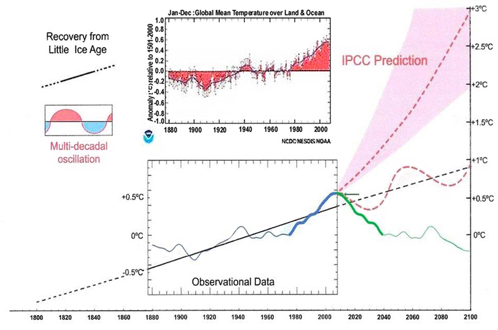
Climate is controlled by natural cycles. Earth is just past the 2003+/- peak of a millennial cycle and the current cooling trend will likely continue until the next Little Ice Age minimum at about 2650.See the Energy and Environment paper at http://journals.sagepub.com/doi/full/10.1177/0958305X16686488
and an earlier accessible blog version at http://climatesense-norpag.blogspot.com/2017/02/the-coming-cooling-usefully-accurate_17.html
Here is the abstract:
“ABSTRACT
This paper argues that the methods used by the establishment climate science community are not fit for purpose and that a new forecasting paradigm should be adopted. Earth’s climate is the result of resonances and beats between various quasi-cyclic processes of varying wavelengths. It is not possible to forecast the future unless we have a good understanding of where the earth is in time in relation to the current phases of those different interacting natural quasi periodicities. Evidence is presented specifying the timing and amplitude of the natural 60+/- year and, more importantly, 1,000 year periodicities (observed emergent behaviors) that are so obvious in the temperature record. Data related to the solar climate driver is discussed and the solar cycle 22 low in the neutron count (high solar activity) in 1991 is identified as a solar activity millennial peak and correlated with the millennial peak -inversion point – in the UAH6 temperature trend in about 2003. The cyclic trends are projected forward and predict a probable general temperature decline in the coming decades and centuries. Estimates of the timing and amplitude of the coming cooling are made. If the real climate outcomes follow a trend which approaches the near term forecasts of this working hypothesis, the divergence between the IPCC forecasts and those projected by this paper will be so large by 2021 as to make the current, supposedly actionable, level of confidence in the IPCC forecasts untenable.”
The forecasts in Fig 12 of my paper are similar to those in Ludecke et al.
DOI: 10.2174/1874282301711010044
It is well past time for a paradigm shift in the forecasting methods used by establishment climate science. The whole dangerous global warming delusion is approaching collapse.
Norman Page,
I agree that it’s mostly natural, at least. And the quasi-cyclic picture looks good to me.
Maybe we don’t have all the cycles identified, and maybe there are inputs that are effectively random, tricking or evading us. If so, these could make predictions unreliable.
But if there’s been a warm spell, a cool spell is likely to follow. Even within an overall long-term warming-trend.
A string of cool years could discredit AGW, whatever causes them, and even to an extent, whatever happens afterward. Not scientifically pretty, but politically potent.
For now, we just watch the monthly T-values come in, and wait.
It’s the average temperature corresponding to the equivalent temperature of the cloud fraction weighted energy emitted by clouds, energy emitted by the surface and surface energy passing through the clouds
all of which passes through GHG’s affecting selective attenuation of specific bands of energy. None the less, the data tells us that on average, the emissions of clouds are linearly related to the temperature of the surface.
I do not agree with the determined commenters insisting this is a great article.
Form a “new” consensus?
That is an absurd strawman.
Consensus severely damages science; especially climate science.
Alarmists use “consensus” as a method to tell people to “shut up”, not as a beacon of science.
Every personal attack leveled at critics of climate science, uses consensus as the guiding principle where naysayers, critics and skeptics are equated to Nazis or traitors.
“Think of your grandchildren!” Phoeey!
What rules of politics are they?
This comes across as somebody’s easy chair assumption, not hard facts.
What about all of the activists that were allowed to enter and control positions of power?
Where are the rules that “politics” can deny grants and loans to scientists that fail to swear fealty to the climate deity?
Most of the American Government takes a very dim view regarding “adjusting” original data to push a position.
The government arm I worked for regularly caught data adjusters, terminated their employment and often filed a criminal case.
Yet, multiple branches of the government have allowed shoddy data handling procedures and actively seek to avoid correcting the irregularities.
Multiple Inspector Generals and Assistant Attorney Generals have cases of their career sitting in front of them; yet they are ignoring the cases
Or is that normal politics too?.
What a mouthful of nonsense!
A) CO2 is a GHG. Big deal. Now prove it as a true function of daily life in weather!
-* That is not a remainder problem, that is a direct prediction followed by absolute and repeatable observations.
B) GHG is making the surface warmer? Not unless proven!
-* To date, normal variance trumps all CO2 warming. This is before asking the climastrologists to explain how CO2 warms three fourths of Earth’s surface, the ocean? Tell me, do you wet noodles to whip the water molecules and surface tension into GHG compliance?
C) Allegedly, based on few measurements; CO2 was as low as 280PPM. Now that metric is around 400PPM.
Placing the emphasis on molecules; that represents 2.8 molecules of CO2 per 10,000 atmospheric molecules rising to 4 molecules per ten thousand atmospheric molecules.
That’s a huge increase of 1.2 molecules of CO2 per ten thousand; yet the alarmists want everyone to be afraid.
That is sad!
D) CO2 is barely a GHG. CO2’s ability to absorb and emit infrared light is restricted to an extremely narrow frequency band. Unlike water that absorbs and emits a very large portion of the available bandwidths.
E) The denier label applies to anyone who doesn’t accept consensus science.
-* Again, not true! The denier label is viciously applied to anyone who might upset the catastrophic apple cart. A playbook ruse directly meant to slander scientists; a ruse taken from various socialist societies and encouraged recently by Strong and Alinsky.
F) Then that wonderful strawman summary, where if everyone doesn’t believe what you claim about CO2, they are in denial and therefore deserve the denier label?
-* Nor does the psychological ploy to cause people to choose joining your side or being “left out”; make any sort of a science argument.
-*
People can believe whatever they want. It is what people can prove or disprove that makes science, not consensus, not group think, not politics, and especially not beliefs; yours or anyone else.
Now prove CO2 GHG effects on today’s temperature! Or tomorrows temperatures.
Not just one spot, but everywhere and at all elevations.
After thirty years of:
• false predictions,
• specious claims,
• weather models that automate disaster predictions,
• Trillions wasted without solid results,
• Publishers’ hijacked,
• CAGW climate team members caught ruining careers, modifying data; for “the cause”.
• Scientists refused publication because they “disbelieve”,
• Science by press release. The dodgier the science, the louder and more widespread the press release,
• Activists ensconced at major news agencies,
• Weather bureaus that fire highly qualified skeptical scientists while retaining or hiring true CAGW believers, so that every weather news is now “climate change”.
• Climate, a science that does not understand nor recognize natural variation; instead they want the MWP wiped off the graph,
• without “adjustments” temperatures are well within normal, worldwide.
• The tide is not rising, unless NOAA applies geoid model calculations, isostatic land rise, whatever first,
• The Antarctic, with it’s faster polar warming, is not melting.
• The Arctic looks to gain ice this year.
• Greenland is gaining ice.
Everything the CAGW CO2 cult has touched is laid waste. Without proving CO2’s actual GHG role in open atmosphere; yet managing to ignore all of the other atmospheric molecules.
“Most skeptics would agree that if there was significant anthropogenic warming”
Really? Got anything to back that up? Because it looks a bit like unadulterated horsesh*t to me.
Bartleby,
If a significant anthropogenic source of catastrophic warming could be proven, I would definitely be for identifying ways to mitigate any damage and so would most of the other people I’ve discussed this with. Of course, like all political issues, there are extremists on all sides who take positions based on insufficient information.
The problem is that alarmists believe this too, but they’re also deluded into believing that that there’s a case to be made for catastrophic warming from CO2 emissions since words like ‘settled’, ‘consensus’ and ‘den ier’ have powerful meanings and these words are echoed relentlessly by an MSM that doesn’t know any better.
Because of my predisposition to act if catastrophic consequences could be proven and as a result of the multi-trillion dollar price tag of mitigation, I decided to do my own due diligence as my education and experience has provided me with the knowledge and tools to do so. The result of that due diligence was that there’s no need for alarm now or in the future and whatever minor warming will result from CO2 emissions is more than offset by the benefits to agriculture of more CO2 and the.benefits of a warmed climate, although a climate warm enough to notice it changed will be hard, if not impossible, to achieve with CO2 emissions.
“If a significant anthropogenic source of catastrophic warming could be proven, I would definitely be for identifying ways to mitigate any damage and so would most of the other people I’ve discussed this with.”
And so, CO2isNotEvil, it would seem the problem is obvious; there is no such evidence?
“it would seem the problem is obvious; there is no such evidence?”
That would be correct. However, there is a lot of evidence to support CO2 as a GHG and that GHG’s warm the surface. There’s also very good evidence, and from my analysis indisputable evidence, that the effect of incremental CO2 while finite, is no more than the lower limit of the effect claimed by the IPCC.
This is the difference between an effect we might want to worry about and and effect we can consider more beneficial than harmful. A catastrophic effect is only an abstract potential consequence of the high end of the presumed sensitivity which is even more impossible than the claimed lower limit.
I might add that, on the heels of a magnificent tomato Caprese dinner, with fresh mozzarella, live basil, extra virgin olive oil, balsamic vinegar, salt and pepper to taste, my sense of imminent doom is greatly diminished.
” However, there is a lot of evidence to support CO2 as a GHG and that GHG’s warm the surface. “
There is conjecture. This isn’t science, and I’ll beg to differ with anyone who says otherwise.
An unquantifiable effect is supposition. The proof, as always, is in the pudding.
“An unquantifiable effect is supposition.”
But the effect of increased GHG’s is quantifiable and I’ve written a full 3-d atmospheric simulator driven by Hitran absorption line data that supports this. This is where my estimate of Fa came from, where I calculated absorption over a range of conditions and then averaged based on the area affected by each condition. If I double Co2, Fa increases a bit and the emissivity drops by about 1.5%, corresponding to a required temperature increase of about 1.1C to achieve the same TOT emissions which is consistent with my assertion that the LTE sensitivity (ECS) is somewhere between 0.2 and 0.3 C per W/m^2 where doubling Co2 is EQUIVALENT to an increase in Pi of about 3.7 W/m^2.
.
Yes, and I can also demonstrate that water, in sufficient quantity is toxic to air breathing life forms; this fact alone does nothing to demonstrate water is toxic.
It’s a losing battle you’re waging CO2, temperature, by any unsullied measure, hasn’t risen during a time when more that 30% of all CO2 ever released by humans in the entire history of measurement, has been released.
No observed effect. You can trundle out all the bell jars you like; there’s no quantifiable effect in the real world.
Bartleby,
It seems that you’re accepting the opposite of the warmist who insist that all of the warming observed since the start of the IR (coincident with the the end of the LWIR) is from man made causes while you insist it’s all natural. I claim that the choice is not between one or the other, but it’s a combination of both.
The effect from CO2 I predict is still less than the warming we have observed since the start of the IR and a significant amount of this must warming still have a natural cause as the rebound from the LIA.
“It seems that you’re accepting the opposite of the warmist who insist that all of the warming observed since the start of the IR…”
No, I’m not accepting I, including your models and lab experiments.
I’ve not observed and increase in temperature coincident with a rise in atmospheric CO2 fraction; not hard. No effect observed. End of conversation.
“A man hears what he wants to hear and disregards the rest”
— Paul Simon, “The Boxer”
Bartleby,
The approximately 0.3C to 0.5C that can be attributed to CO2 during the last 150 years is barely at the level of a temperature change perceptible to ordinary human senses and that would be if you’re lived for 150 years to have observed the change. But then again, the curvature of the Earth is also mostly beyond the ability of human senses to detect.
There’s a big difference between no effect whatsoever and a small, inconsequential effect. Asserting the former is what leads to the de nier label while the later is supported by physics and is consistent with both sides of the science.
Pretty much the same findings that everyone who’s looked at the matter independently came to.
CO2isnotevii:
In your reply to Bartleby (Aug. 21, 6:51 pm), you wrote “:If a significant anthropogenic source of catastrophic warming could be proven, I would definitely be for identifying ways to mitigate any damage”
Actually a proven anthropogenic source which can lead to catastrophic warming DOES exist.
The mechanism is the removal of dimming anthropogenic Sulfur Dioxide emissions from the atmosphere due to Clean Air efforts.
This is fully discussed in my on-line post “Climate Change Deciphered”, which can be viewed by Googling the title. (It should be added that all El Ninos are due to reductions in atmoospheric SO2 levels – a later discovery).
Since there is currently around 80 Megatonnes of anthropogenic SO2 emissions in the atmosphere, continued reductions in that amount could lead to approx. 2 deg. C. of catastrophic additional warming.
With respect to mitigation, all that needs to be done is to halt all additional efforts to reduce SO2 emissions (insofar as possible)
Burl,
Your hypothesis seems to be based on the high sensitivity claimed by the IPCC. If a more rational sensitivity is applied, the effect on temperature will be significantly reduced.
co2isnotevil:
You state “Your hypothesis…”
No, it is not a hypothesis, just a correlation of existing facts.that has escaped everyone until now.
You obviously did not read (or understand) my on-line post, or you would not have commented as you did.
A full 3-D atmospheric simulation?
One that includes all of the gases, in their proper proportions, including water?
One that recognizes the very limited absorption/emission spectra available to CO2?
How did you randomize the infrared emission direction?
Did every molecule receive an infrared emission that was explicitly emitted by surface or atmospheric molecules?
Or was there a general equation fudging the absorption/emission/absorption rates?
Somehow, I doubt the 3-D model is an exact replication of atmosphere. leaving the latter case more likely.
It still comes down to, proved a definitive prediction that can be proven by observations.
That is your personal problem, not mine, not ours, not anybody else’s. It is your choice of fears.
If there were possible catastrophic consequences” Based on what historical references?
When have higher CO2 levels or higher Earth temperatures ever caused “catastrophic consequences”?
Forget using the specious correlations used by climastrologists trying to infer CO2 caused extinctions. In each case, the climastrologists string together ever more unlikely scenarios while ignoring immense gaps in timelines.
It falls back to prove it or move on with your “the Earth is ending” placards.
Warmer periods are termed “optimums”, for very good reasons. It is the cold periods that are deadly to life and humans.
Even blaming mankind for the CO2 increase, mankind has only managed 1.2 molecules of CO2 per ten thousand atmospheric molecules over the past century.
That people have unreasonable expectations for those 1.2 CO2 molecules is severe understatement.
A full 3-D atmospheric simulation?
I can dial in as many horizontal slices as I want and any grid size. It happens that when you reach a certain number of layers and a small enough grid size, taking it to the limit doesn’t change the results. The larger the grids and the smaller the slices, the more digits of precision are generated and the long the computations take. Obviously, you don’t need many digits of precision …
One that includes all of the gases, in their proper proportions, including water?
The gases I included, in order of importance, were, H2O, CO2, O3, CH4, N2O, CO and even O2 absorption.
One that recognizes the very limited absorption/emission spectra available to CO2?
It was driven by HITRAN line data which does this implicitly.
How did you randomize the infrared emission direction?
By insuring that as a bulk property and absent of clouds, the flux of energy absorbed by GHG’s leaving the top of the atmosphere was equal to that being returned to the surface.
Did every molecule receive an infrared emission that was explicitly emitted by surface or atmospheric molecules?
Obviously not every molecule by itself, but as a statistical population, yes, however only the water in clouds and GHG’s emit any appreciable amount energy within the atmosphere.
Or was there a general equation fudging the absorption/emission/absorption rates?
No.
BTW, no simulation of the atmosphere is exact, the best we can do is approximate it, but given enough information, it’s possible to get arbitrarily close.
Unadulterated? What adulterants were tested? Where’s the data?
You just need to test the horsesh*t for adulterants Ted. If it’s not pure horsesh*t it will be obvious.
Yeah, it’s hard to find qualified testers. There are standards, and tests!
Today, there are very few skeptics. And many are facultative, expressing themselves variably, depending on the environment.
But tomorrow there will be billions of long-time skeptics, dyed in the wool for decades.
Where’s the purity-fraction then? It’s not an easy mission, Bartleby.
Ted, I’m a horse breeder. I know my horsesh*t.
I have to agree with the above series of exchanges.
For sure, CO2 is a radiative gas, the laboratory properties of which are known, but there is no evidence that it is a GHG, at any rate at levels exceeding about 200 ppm. It is mere supposition and conjecture that CO2 is a GHG. It maybe, or it may not be but only proper observational empirical evidence will establish that.
I even have issues with temperature rise since the 1940s. I would wish to see a proper re-measurement of the NH before I would accept that today the NH is any warmer than it was in the late 1930s/1940s.I am far convinced that there has been any significant warming these past 75 or so years. For sure there has been multidecadal variation, but I am far from convinced that the globe in 2017 is any warmer than it was in the late 1930s/early 1940s notwithstanding the fact that this period encompasses some 95% of all manmade emissions.
” … but there is no evidence that it is a GHG, at any rate at levels exceeding about 200 ppm …”
This not true. A true statement would be “but there is no evidence that it has a GHG effect, radiant or otherwise, as large as the IPCC claims at any concentration”.
There’s definitely evidence that the incremental effect due to increasing GHG concentrations is not zero, both as theory and by experiment. While the effect gets smaller as concentrations rise, it never drops to zero.
They’ve clearly over-estimated the sensitivity by a wide margin and it seems likely that they also over-estimated the equivalent forcing of doubling CO2 concentrations by not accounting for incremental absorption by the atmosphere that’s ultimately emitted into space. I haven’t addressed the equivalent forcing issue because its not necessary given by how much they over-estimated the sensitivity.
riichard verney:
Average global temperatures in 2017 are clearly higher than they were in the late 1930’s and early 1940’s, with NH.temperatures being even higher
For a complete explanation of what has happened to Earth’s climate since 1850, Google “Climate Change Deciphered”..
Something else I’ve noticed is that the IPCC and its ‘consensus’ has been adding layer upon layer of obfuscation to the concept of sensitivity and perhaps this is confusing many, as this is what the goal seems to have been.
One thing Hansen did get more or less right with his feedback paper was to express gain (sensitivity) as the dimensionless ratio of W/m^2 of surface emissions per W/m^2 of forcing. Schlesinger changed this along with his ‘corrections’ for Hansen’s other errors, to be a change in temperature per W/m^2 of forcing.
The most relevant sensitivity from AR1 was the sensitivity factor of 0.8C +/- 0.4C per W/m^2 where doubling CO2 was equivalent to 3.7 W/m^2 of solar forcing, keeping the system constant and even then it was detached from the more meaningful and far less plausible metric of 4.3 W/m^2 of incremental surface emissions per W/m^2 of forcing. Schlesinger changed the dimensions of the metric in order to add the conversion from W/m^2 to T as part of the open loop gain (and then undo it to calculate feedback) and to differentiate between the asserted sensitivity as being incremental and the average sensitivity of only 1.6 W/m^2 of surface emissions per W/m^2 of accumulated solar forcing.
Somewhere along the line, the sensitivity was reinterpreted to be the temperature effect from doubling Co2, combining the 0.8 +/- 0.4 sensitivity factor and the 3.7 equivalent forcing into a single metric.
The more recent layer of obfuscation are the various RCP scenarios where the number following RPC is the presumed forcing in W/m^2 with a temperature effect is still assumed to be 0.8 +/- 0.4C per W/m^2, where the CO2 increase is backed out assuming 3.7 W/m^2 of equivalent forcing per doubling. The scenarios are further expressed as representing various scenarios assuming business as usual, blah, blah, blah.
WTF
Hi George
I did not manage to read through all of it, and mostly I could not wrap my had around all you are saying. The funny thing however is, that quite a number of parts could have been taken from my essay..
https://www.scribd.com/document/348761444/Its-the-Ocean-Stupid
Note: my essay contains one major mistake, making it pretty useless as it is. Ocean water emissivity is not what I calculated it to be (~0.84), but rather 0.94. So I will need to rewrite it anyhow.
Yet it contains a lot of usefull facts, and most notably the model still works, with the best part being my analysis of weather data to determine the magnitude of cloud forcing.
Note that if cloud forcing was only about 30W/m2 (like the IPCC claims), and we assumed clouds to cover an average 30% of the surface, we could assume 30/0.3 = 100W/m2 of cloud forcing for an all overcast sky.
Now average emissions will be about 236W/m2 (corresponging to amount solar radiation received 342*(1-0.31) in this case), and that will be down from about 390W/m2 the surface would emit at its given average temperature. The the total “GHE” would amount to 390 – 236 = 154W/m2. Yet this would be including cloud forcing. Without clouds, average emissions would then rather be 236 + 30 = 266.
So an all overcast sky should reduve emissions by 100/266 = 37.6% vs. a clear sky. But that is not what we can observe. Rather I had the impression, that nocturnal cooling was much more strongly impaired by clouds, at least by up to 2/3s or so.
So had to analyze weather data to some usefull and quantifiable results. This is what it looks like:
http://i736.photobucket.com/albums/xx10/Oliver25/parkersburg1.png
Without going through the details hereto, it shows that cloud forcing must be massive. An all overcast scenario is diminishing night time cooling by a 85%. On average however, and I discussed this in my essay, clouds seem to impair emissivity by a 35%.
35% of 266W/m2 would be 93W/m2. However that includes the assumption of cloud forcind being only 30W/m2, which does not hold true, obviously. We could solve that by an iterative process, or just bring up a reasonable formula. With x standing for cloud forcing, the equation would be x = 0,35 * (236 + x), which is true for x = 127.
So cloud forcing amounts to 127W/m2, that is out of a GHE of 154W/m2. That would leave only 27W/m2 for the remaining GHE, but only of surface emissivity was indeed 1. Emissivity however is less than 1, and if we take a chance and include clouds with the surface (as we do when we talk about absorptivity), then it is (236 + 127) / 390 = 0.93.
As emissivity of water is about 0.94, and land has definitely a lower emissivty, this figure seems to satisfy it all. With a surface emissivity of 0.93 (a drop of 27W/m2 vs. a perfect black body), and a cloud forcing of 127W/m2, the total GHE of 154W/m2 is explained. And that is without any green house gas.
Leitwolf,
Yes the warming effect from clouds is more than 30 W/m^2. The top of clouds have an emission temperature of about 265K with corresponding to emissions over 240 W/m^2, which even adjusted down for emissivity is far more than 30 W/m^2 since an approximately equal amount of energy must be directed back down to the surface.
One thing to be wary about cloud coverage is that it must be specified as some average emissivity. For example, the 66% of the surface covered by clouds in the ISCCP data is based on average clouds having an emissivity of about 0.72 as this also encompasses a significant fraction of partly cloudy conditions. If instead, you selected the cloudy threshold to have an average emissivity of 0.9, the fraction of the surface covered by clouds would be much less.
To co2isnotevil. It looks like that you are capable to carry out spectral analyses using line-by-line calculations.. It also looks like that you have never questioned the RF formula of Myhre et al., which is the basis of IPCC’s simple model and all GCMs (that is why their results are almost the same). The evidence is not in the fact, that it has been used in so many research studies. This was the answer what I got from Harde, when I asked, why he is using the Myhre’s formula. I recommend you carry out or reproduce the original study of Myhre et al. I did, and I got a different result, link: http://www.seipub.org/DES/paperInfo.aspx?ID=17162
In doing so, the calculation will give the answer directly, what is the surface temperature increase needed to increase the surface emitted LW radiation in order to keep the ourgoing LW radiation in the same value for CO2 concentration of 560 ppm as it was for the value of 280 ppm. The climate sensitivity of my calculations were 0.6 Celsius degrees. A funny thing is that Myhre et al. did not show this temperature value but only the RF values. The calculations must be carried out by trial and error, because otherwise it is not possible to find out the outgoing radiation value being exactly the same for two CO2 concentrations 280 ppm and 560 ppm.
This is something I did a long time ago and have a table of this somewhere and code to reproduce it, but its late here now, so I will look at it tomorrow. If I recall, I had to increase the surface temp by less than 1C to achieve the same energy at TOT after doubling Co2 and no where near the 3C claimed by the IPCC.
aveollila,
This was something I did way back in 2010 and I can’t seem to find table, which is probably on one of my decommissioned computers. It would probably be easier to reconstruct this which I will put on my list of things to do and try to get to it over the next few days.
I did find some a log of some clear sky results for the difference between 280 ppm and 560 ppm, but this didn’t have the results from adjusting the surface temp to equalize emissions. One of the things that I noticed, but had forgotten about was that as CO2 absorption increases, H2O absorption decreases owing to the overlap between the two sets of absorption lines. The H2O absorption decrease is equal to about 20-25% of the CO2 absorption increase.
aveolilla,
“what is the surface temperature increase needed to increase the surface emitted LW radiation in order to keep the ourgoing LW radiation in the same value for CO2 concentration of 560 ppm as it was for the value of 280 ppm.”
If assumed that the 3.7 W/m^2 of RF is equal Pi (post albedo solar power in), it would be about 1.1C intrinsically, but this assumption is almost certainly wrong; and half of that or around 0.55C is probably correct. This is because the 3.7 W/m^2 is just the additional instantaneous up IR capture from the surface, and is henceforth re-radiated both up and down in the atmosphere in roughly equal proportions (i.e. henceforth acts to both warm and cool in roughly equal proportions).
co2isnotevil has devised a black box exercise to quantify for this and it yields/supports that it is pretty close to half, or for 2xCO2 only about 0.55C of theoretical intrinsic surface warming ability.
Modeling the GHGE.
1. You cannot model an average. Behavior changes depending on latitude, time of day, and season, etc. E.g. At the poles the ratio of CO2:H2O is about 1:1. At the equator the ratio is more like 1:1000. Whatever changes the ratio of CO2:H2O changes how the GHGE works.
2. To the best of my knowledge the alarmist description of how the GHGE works is wrong. I’ve been told “the photon absorbed is immediately re-emitted”. That is demonstratively false. The photon absorbed is thermalized because re-emission takes many milliseconds. Each millisecond sees an air molecule experience about 1 million collisions with other air molecules. So the energy absorbed must be shared about. In those circumstances I don’t see how re-emission can happen at the same frequency. It seems likely to me that radiative emissions from air will tend to happen at lower energies. Because more molecules have that much energy available. I believe water vapour has many such low energy bands. All this makes modeling the GHGE quite difficult. I’d love to know what Will Happer has to say about the fine detail of this!
Given all this, I’m not surprised alarmists obfuscate everything they do. To be convinced by alarmists GHGE predictions I want to see the science they did on points 1 & 2 (above). Science = data collection and experiment; not hypothetical modeling based on inadequate understanding and data.
Ooops. 1:100 not 1:1000
Of course you can model an average, and I guess it’s much easier to do that than try a real simulation. Problem is: the result you get does not really have any real world meaning. That’s what I really meant by can’t model an average. Once you start modeling averages, you need to demonstrate the result makes sense by validating it against the real world.
““the photon absorbed is immediately re-emitted”. I do not know from which source, this quotation is coming, but it is wrong. If a photon has been absorbed and then re-emitted immediately, there is actually no absorption. In absorption process, a photon is absorbed, it creates mechanical movements between atoms of this GH gas molecule, which means increase of thermal energy, and thereafter this molecule re-emits another photon with lower frequency, which means a lower energy level.
mark,
“You cannot model an average. Behavior changes depending on latitude, time of day, and season, etc.”
I’m measuring changes in the yearly average of adjacent slices of mid latitude, close to the slices which have an average temperature representative of the average of the whole. The poles do get squirrelly, especially during winter months, but the poles represent only a small fraction of the area of the planet.
“The photon absorbed is thermalized because re-emission takes many milliseconds. Each millisecond sees an air molecule experience about 1 million collisions with other air molecules.”
Except that no energy is converted between the state energy of an energized GHG molecule and the kinetic energy of translational motion by a collision. Quantum mechanics requires the entire quanta of absorbed energy be absorbed or emitted as a single event so the most likely event is that a collision will cause an energized GHG molecule to emit a photon and return to the ground state. The photon of energy is never ‘thermalized’ unless it happens to be absorbed by the liquid or solid water in clouds, or the sensor of a thermometer, and the entire quanta is thermalized at once. Of course, each re-emission pair involves a new photon of the same energy as the absorbed photon.
The exception is collisional broadening, where small amounts of energy can be added to or subtracted from the photon energy and added or subtracted from the energy of the collision resulting in the absorption or emission of a photon a little bit on either side of the central resonance. Since this has an equal probability of subtracting from or adding to the collision energy, no net ‘thermalization’ occurs. Besides collisional broadening is a low probability event at the relatively low pressures found in the atmosphere.
co2isnotevil August 21, 2017 at 11:38 pm
“The photon absorbed is thermalized because re-emission takes many milliseconds. Each millisecond sees an air molecule experience about 1 million collisions with other air molecules.”
Except that no energy is converted between the state energy of an energized GHG molecule and the kinetic energy of translational motion by a collision. Quantum mechanics requires the entire quanta of absorbed energy be absorbed or emitted as a single event so the most likely event is that a collision will cause an energized GHG molecule to emit a photon and return to the ground state. The photon of energy is never ‘thermalized’ unless it happens to be absorbed by the liquid or solid water in clouds, or the sensor of a thermometer, and the entire quanta is thermalized at once. Of course, each re-emission pair involves a new photon of the same energy as the absorbed photon.
Not true, when an IR photon is absorbed by a CO2 molecule its vibrational and rotational levels are increased, collisions can remove energy and reduce the ro/vib to lower levels. At atmospheric pressure the number of collisions is so high that the most likely result is that the excited state is deactivated by exchange to the surrounding gas molecules. High up in the atmosphere at lower pressure the collisional deactivation rate is lower so it is more likely that a photon will be emitted. The entire original exciting quantum does not have to be thermalized at once.
Phill,
The rotational states of CO2 are in the microwave region and have very low energies. These are responsible for the fine structure in the absorption spectrum, but this fine structure is symmetric on either side of the primary lines which means that energy can be either added to or subtracted from rotational states upon the absorption or emission of a photon so to the extent that rotational state energy itself can be converted into translation motion, it works both ways and the net is zero.
co2isnotevil August 22, 2017 at 8:40 am
Phill,
The rotational states of CO2 are in the microwave region and have very low energies. These are responsible for the fine structure in the absorption spectrum, but this fine structure is symmetric on either side of the primary lines which means that energy can be either added to or subtracted from rotational states upon the absorption or emission of a photon so to the extent that rotational state energy itself can be converted into translation motion, it works both ways and the net is zero.
No. When CO2 absorbs a photon in the 15 micron band it is excited from a rotational level in the ground vibrational level to another rotational level in the v=1 vibrational level. Let’s take it’s the v=1, J=7 level, 96% of the colliding molecules have a lower kinetic energy than that so energy can be chipped away a level at a time by the thousands of collisions that occur during the radiational lifetime of the excited state. The normal selection rules don’t apply to collisional deactivation. While it is possible that some energy can be added the net effect is a decrease in energy, this has been observed in fluorescence studies. The CO2 laser relies on collisional deactivation of the lower state by Helium to achieve population inversion.
Phil,
“so energy can be chipped away a level at a time by the thousands of collisions”
No. The energy stored as state energy is stored as a resonant wave in the E-fields of the molecules electron cloud. Once you remove a little bit of the energy and move away from resonance, the probability of spontaneous emission starts to increase dramatically. Quantum Mechanics precludes what you say is occurring and dictates that the entire quanta of state energy must be be emitted or transferred in a single event. This means either emitting a photon or exchanging state with another similar GHG molecule. Conditions can push resonance a little bit on either side, but no where near far enough to maintain the state when energy is ‘chipped away’ a tiny bit at a time.
co2isnotevil August 23, 2017 at 10:45 am
Phil,
“so energy can be chipped away a level at a time by the thousands of collisions”
No. The energy stored as state energy is stored as a resonant wave in the E-fields of the molecules electron cloud. Once you remove a little bit of the energy and move away from resonance, the probability of spontaneous emission starts to increase dramatically. Quantum Mechanics precludes what you say is occurring and dictates that the entire quanta of state energy must be be emitted or transferred in a single event. This means either emitting a photon or exchanging state with another similar GHG molecule. Conditions can push resonance a little bit on either side, but no where near far enough to maintain the state when energy is ‘chipped away’ a tiny bit at a time.
I think you need to study some quantum mechanics, we are talking about rotational and vibrational transitions not electronic transitions. If what you said was true there would no ‘Stokes shift’ in fluorescence photography.
https://en.wikipedia.org/wiki/Stokes_shift
http://www.public.asu.edu/~laserweb/woodbury/classes/chm467/bioanalytical/spectroscopy/Image384.gif
Phil,
“… we are talking about rotational and vibrational transitions not electronic transitions.”
No we’re not. We’re talking about solutions to Schroedinger’s Wave equation. While this is far easier to apply when describing photon absorption and emission of something simple like a Hydrogen atom, none the less, the basic concepts described by this equation apply to the absorption and emission of photons to/from any atom or molecule. Why do you think gases have absorption lines and not an absorption continuum like that exhibited by solids or liquids?
You seem to be conflating the kinetic energy of mass in motion with quantized state energy stored as a resonant wave in the electron cloud of an atom or molecule. These two forms of energy are not arbitrarily interchangeable.
co2isnotevil August 23, 2017 at 12:04 pm
Phil,
“… we are talking about rotational and vibrational transitions not electronic transitions.”
No we’re not. We’re talking about solutions to Schroedinger’s Wave equation. While this is far easier to apply when describing photon absorption and emission of something simple like a Hydrogen atom, none the less, the basic concepts described by this equation apply to the absorption and emission of photons to/from any atom or molecule. Why do you think gases have absorption lines and not an absorption continuum like that exhibited by solids or liquids?
You seem to be conflating the kinetic energy of mass in motion with quantized state energy stored as a resonant wave in the electron cloud of an atom or molecule. These two forms of energy are not arbitrarily interchangeable.
Your interpretation of QM is unable to explain the reality of what happens. The idea that the vibrational state of a molecule is a resonant wave in the electron cloud is nonsense, it is the nuclei that are moving. Explain the observations in Fig. 5.
http://pubs.acs.org/doi/pdf/10.1021/ed059p446
Phil,
What about this relates to how GHG’s operate in the atmosphere? The energy densities for laser induced florescence don’t occur in the atmosphere, except perhaps in a bolt of lightning. Even a 30 mw laser focused on a 10 mm^2 spot has an energy density of 3000 W/m^2. It’s important to understand that all of my comments are related to what’s happening in the atmosphere that’s being modelled by the top down behavioral model.
Certainly, at high enough temperatures, collisions can induce energized states, but again, I’m focusing on what happens in the atmosphere, not what happens under more extreme conditions. In a particle accelerator, translational energy from colliding particles is converted into streams of high velocity particles, i.e. converting energy to fast moving mass, but this doesn’t happen in the atmosphere either except when the odd cosmic ray or when particles from a CME interacts with molecules high up in the atmosphere.
I’ve also become more convinced that there are 2 kinds of ‘rotation’. One is a physical rotation of mass which can rotate at any speed and for all intents and purposes is not quantized and that this is the rotational degree of freedom that can readily exchange energy with spatial degrees of freedom. The other is more like spin where only the electrons E-fields are rotating in a resonant state where the allowed energies are clearly quantized and the rotation rate is very fast with periods on the order of a sub-harmonic of the Compton Frequency. At the energy densities found in the atmosphere, this can only exchange energy with other EM states, for example, vibration.
Pedantic theory suggests that Equipartition of Energy applies in the limit, but clearly, this is a macroscopic property of the aggregate and does not apply individually to molecules, moreover; the energy of the photons involved with GHG absorption and emissions are already about the same as the kinetic energy of molecules in motion, thus is already equalized. Presuming that the arbitrary conversion between these two types of energy is required for conformance to Equipartition of Energy, which isn’t even required since they are already equalized in the bulk, seems to be the origin of climate science errors related to ‘thermalization’. Measurements of the emitted spectrum of the planet also contradict the idea that any significant amount of ‘thermalization’ is occurring. If it was, we would expect nearly infinite attenuation in the absorption bands, yet we only observe about a 3db reduction (a factor of 2).
You didn’t answer my question about the significance of the impedance quantified by 2h/q^2 which is fundamental to why allowed state energies are constrained by resonances. I’ll give you some more hints. The ratio between the impedance of free space and this impedance is the only dimensionless physical constant. One more hint is that it can be derived by EQUIVALENTLY modelling photons and electrons as obeying Maxwell’s Equations.
co2isnotevil August 24, 2017 at 9:54 am
Phil,
What about this relates to how GHG’s operate in the atmosphere? The energy densities for laser induced florescence don’t occur in the atmosphere, except perhaps in a bolt of lightning. Even a 30 mw laser focused on a 10 mm^2 spot has an energy density of 3000 W/m^2. It’s important to understand that all of my comments are related to what’s happening in the atmosphere that’s being modelled by the top down behavioral model.
The QM is the same, the advantage of using the laser is the ability to tune the exciting wavelength to excite a single state and study its subsequent behavior. Just because there are more photons doesn’t change what happens. You keep referring to electrons, we’re not talking about electronic transitions, the transitions in the IR are rotational-vibrational motions of the atoms in the molecules. These motions are quantized but can still exchange energy by collisions with other molecules, mostly the energy is transferred to the translational motion of the collision partner but can also involve vibrational modes if there is a matching energy separation, e.g. N2 to CO2 in a CO2 laser.
moreover; the energy of the photons involved with GHG absorption and emissions are already about the same as the kinetic energy of molecules in motion, thus is already equalized.
Actually at 300K only about 4% of the molecules have kinetic energy equal to or more than the photon energy the majority are significantly lower, at 220K it’s more like 1%.
When we are taking about GHG absorption and emission, we are definitely talking about electron shells absorbing and emitting photons. When an atom or molecule absorbs a photon, that energy is added to or subtracted from the energy of the electrons. This is why only photons with specific energies and not all energies can be absorbed. The energy has to ‘fit’ within the molecules shared electron fields and if you add enough, you can disassociated the atoms in the molecule.
From E = hv, the energy of a 15u photon, which in the middle of the major CO2 absorption band, is about 1.3E-20 joules. From E = 1/2mv^2, the average velocity of an air molecule is about 500 m/sec and the mass of a CO2 molecule is 44 AMU or about 7E-26 kg making its kinetic energy 8.8E-21 which is only about 10% less then the photons involved with CO2 absorption, so its a lot closer than you think.
co2isnotevil August 24, 2017 at 11:18 pm
When we are taking about GHG absorption and emission, we are definitely talking about electron shells absorbing and emitting photons. When an atom or molecule absorbs a photon, that energy is added to or subtracted from the energy of the electrons. This is why only photons with specific energies and not all energies can be absorbed. The energy has to ‘fit’ within the molecules shared electron fields and if you add enough, you can disassociated the atoms in the molecule.
The main absorption band of CO2 in the atmosphere is the bending mode, the energy absorbed causes the molecule to bend, i.e. the atoms are caused to move in space relative to each other.
Here’s a nice illustration of the CO2 bending mode:
http://www.chemtube3d.com/vibrationsCO2.htm
From E = hv, the energy of a 15u photon, which in the middle of the major CO2 absorption band, is about 1.3E-20 joules. From E = 1/2mv^2, the average velocity of an air molecule is about 500 m/sec and the mass of a CO2 molecule is 44 AMU or about 7E-26 kg making its kinetic energy 8.8E-21 which is only about 10% less then the photons involved with CO2 absorption, so its a lot closer than you think.
I was taking T=220K since we were talking about the stratosphere, in which case the average kinetic energy is: 0.455E-20 J
Only about 1.4% of the molecules have kinetic energy more than 1.3E-20 J
A CO2 molecule with the average kinetic energy will have an rms velocity of ~350 m/s (N2 ~440 m/s)
For 300 K the corresponding values are:
0.62E-20 J
4%
412 m/s
In other words it isn’t as close as you think.
Phil.
” … the atoms are caused to move in space relative to each other.”
It’s only the electron shell bending around nuclei that remain relatively stationary. The vibrations are very fast and the inertial of the nuclei prevents them from moving very far. Keep in mind that the diameter of an atom (1E-10) is about 5000 times greater than the diameter of the nucleus (2E-15).
Relative to the energy balance and the sensitivity, which is all I’m concerned about here, the stratosphere is mostly irrelevant as most of the planets emissions originate at lower levels in the atmosphere, moreover; most of the GHG effect that’s related to the surface temperature occurs in the lower troposphere.
Phil,
If your point of view is correct, why don’t we see narrow band absorption converted into broadband (Planck) emission, as we would in liquid or solid? This is the basic question that I’ve yet to see anyone actually answer who thinks the absorbed IR in the atmosphere is ‘thermalized’ by collisions with the non-GHG molecules.
You are aware that the only way the mainstream view or theory of atmospheric radiation works is if Kirchoff’s law is applied to each wavelength independently (except if absorbed by the condensed water in clouds), right?
If the end result of the physics is different, there has to be different physics occurring, otherwise the result would be the same whether one is dealing with a liquid, a solid, or a gas. But it’s not the same.
RW,
Exactly correct. The assumption that Kirchoff’s Law and Equipartition of Energy must be adhered to at the limit (i.e. as the space delta goes to zero) seems to be the fundamental problem. Both of these are bulk properties and not properties of individual atoms or molecules. It’s all about statistical distributions and not absolutes.
RW August 25, 2017 at 8:52 am
Phil,
If your point of view is correct, why don’t we see narrow band absorption converted into broadband (Planck) emission, as we would in liquid or solid? This is the basic question that I’ve yet to see anyone actually answer who thinks the absorbed IR in the atmosphere is ‘thermalized’ by collisions with the non-GHG molecules.
Because the physics of the condensed phases are different from the physics of gases. Typically gases have line spectra, if you illuminate CO2 with a single wave length at low pressure you’ll get a few lines emitted from that energy level. Add a little N2 and you’ll get multiple lines from the original level and other lower levels which have been populated by collisions. Add more N2 and the emission lines disappear because the energy is all transferred to the translational modes of the N2. Even if by chance the energy was transferred to a vibrational mode of a N2 molecule (would require an highly excited CO2 molecule) there still wouldn’t be an emission because N2 doesn’t emit at that wavelength.
If the end result of the physics is different, there has to be different physics occurring, otherwise the result would be the same whether one is dealing with a liquid, a solid, or a gas. But it’s not the same.
Exactly, the physics is different.
Phil.
The effect you are seeing is that when a collision occurs and the energy is high enough, lower energy states can be energized or returned to the ground state by emission, with equal probability. Another effect is that a collision with an energized molecule can result in not all of the energy being emitted as a photon, but a fraction of the energy can be retained to energize a lower energy state, for example, the uwave rotation bands of CO2. To the extent that energy is added to the linear kinetic energy, it’s also removed in equal and opposite amounts so the net average is zero.
One experiment you should try is to see what the emission spectra looks like when the heat applied is coming from a laser in the transparent region of the spectrum. If the laser is tuned slightly above or below the primary line without increasing the likelyhood of collisions, you will see more emissions in the lower energy bands. And of course, the total energy involved in the uwave region is such a tiny fraction of the whole, any net exchange would be imperceptible anyway.
BTW, we do see a small amount of thermalization from water vapor, as energized water vapor molecules condense and add their energy to the condensing water droplet. We see this as a slightly higher attenuation (about 4 db, rather than 3 db) in the most saturated water vapor lines.
Phil,
Something else to try is to add up the energy of the emissions before and after adding the N2 and see if the total emitted energy changes. It thermalization is occurring, the total should be much less. If collisions are adding to the emissions, you should see more power being emitted. If neither of these is happening, or they are happening in equal and opposite amounts, the total emitted power will be the same and just redistributed across other wavelengths.
co2isnotevil August 25, 2017 at 11:07 am
Phil.
” … the atoms are caused to move in space relative to each other.”
It’s only the electron shell bending around nuclei that remain relatively stationary. The vibrations are very fast and the inertial of the nuclei prevents them from moving very far. Keep in mind that the diameter of an atom (1E-10) is about 5000 times greater than the diameter of the nucleus (2E-15).
The electron shell remains fixed with respect to the nucleus but the vibrational mode involves the relative motion of the nuclei. Best modeled as an anharmonic oscillator but can be approximated at low levels as an harmonic oscillator (mass and spring). Regardless the of the inertia it’s still the nuclei that move, bear in mind that for CO2 they’re on average 116 pm apart.
http://www.chem.purdue.edu/courses/chm424/Handouts/16.1%20Molecular%20Vibrations.pdf
Relative to the energy balance and the sensitivity, which is all I’m concerned about here, the stratosphere is mostly irrelevant as most of the planets emissions originate at lower levels in the atmosphere, moreover; most of the GHG effect that’s related to the surface temperature occurs in the lower troposphere.
As shown above your assertion was still wrong, 96% not 99% but still a long way from 50%!
Phil,
Here’s the calculation that shows how the nucleus isn’t moving by very much as a CO2 molecule vibrates:
For the Oxygen atoms in a CO2 molecule, the total force acting between the nucleus and the electron shell is given by,
F = e0*q^2/d^2
e = 8.85E-12
q = 8*1.6E-19 = 1.3E-18
d = 1E-10 meters (approx distance from nucleus to electrons)
F = 1.5E-27 Nt.
The fraction of this that can arise by bending the electron shell by the amount that occurs in a CO2 molecule is than 25% of the total force, but lets consider the entire force is acting on the nucleus.
mass of Oxygen atom = 16amu = 2.6E-26 kg
The acceleration acting on the nucleus is a = F/m
a = 5.8E-2 m/sec^2
The distance between the center of the nucleus and the electron shell is about 1A or about 1E-10 m. The most it would need to move is about 20% of this distance, or 2E-11 m.
d = a*t^2/2
for d = 2E-11 and a = 5.8E-2
t = sqrt(2*d/a) = 2.5E-5 seconds
This is about 25 us corresponding to a frequency of only 38 Khz.
Half of the 5E-14 second period of a 15u photon, which approximately corresponds to the period of vibration that results, is no where near enough time for the nucleus to move 2E-11 m and at the most, it will move by about a millionth of the distance between the nucleus and the electron shell. Even less considering that only a fraction of the total electrostatic force will be acting on the nucleus and there are on other forces acting on the nucleus to make up the difference.
Even at the frequency of the rotational states, little movement will result. However; the movement of mass, for example the same kind of physical rotations that say an atmospheric O2 or N2 molecule will exhibit, are slow enough that the nucleus will be dragged along for the ride.
co2isnotevil August 25, 2017 at 12:14 pm
Phil,
Something else to try is to add up the energy of the emissions before and after adding the N2 and see if the total emitted energy changes. It thermalization is occurring, the total should be much less. If collisions are adding to the emissions, you should see more power being emitted. If neither of these is happening, or they are happening in equal and opposite amounts, the total emitted power will be the same and just redistributed across other wavelengths.
In my LIF experiments with OH the emitted signal dropped significantly as pressure was increase until there was no observable signal. That’s why it’s often referred to as quenching!
“Suffers from quenching, i.e. collisional deexitation quantitative species concentration measurements not trivial”
From: https://www.princeton.edu/cefrc/Files/2011%20Lecture%20Notes/Alden/Lecture-5-LIF.pdf
Phil,
Are you saying the total emitted energy dropped to zero, or did it all just get transferred into other bands? If total emissions dropped to zero, you wouldn’t see any emissions anywhere in the spectrum. Based on the figures in the paper, it looks like the energy in the central line is just getting moved into the fine structure on either side. The emissions you’re measuring also don’t look like they include the uwave emissions as the molecule returns to the ground state from rotation states, although some of this is seen indirectly as the emissions at energies higher than the primary line as both rotational and vibrational states return to the ground state at once.
The pulsed nature of the setup also seems a little problematic. A 1 us pulse with a 10 Hz rep rate isn’t necessarily representative of the steady state behavior under continuous excitation where the system is not given a chance to cool.
Phil,
“Because the physics of the condensed phases are different from the physics of gases.”
Yes, I know that. What I meant was the line of succession of physical processes is claimed to be the same for all three states of matter, yet the end result is different. You are aware that the mainstream view of atmospheric radiation doesn’t differentiate their use and definition of the manifestation of LTE in the atmosphere compared to that of a liquid or solid, correct? It’s all claimed to be the same.
The claimed line of succession of physical processes is that the absorbed photonic energy is converted/transferred into the mechanical energy of molecules in motion via collisions with non-GHG molecules and then subsequently transferred back to photonic emission via collisions, right? This is also what is agreed to happen in a liquid or solid in LTE, right? That is, collisions equalize everything and manifest LTE the same was as it would in a liquid or solid.
Now, we come to my question that as of yet I’ve not seen anyone be able to provide an answer. That is, in the atmosphere, there’s no narrow band absorption converted into broadband Planck emission (as would universally occur in liquid or solid absorbing and emitting radiation).
That is, if we define end result A as matter in LTE with absorbed and emitted radiant flux, in order to predict the emitted spectrum for a liquid or solid, Planck’s law (in conjunction with Wien’s displacement law) is what has to be applied in order to predict the correct emitted spectrum, REGARDLESS of the wavelength distribution absorbed by the matter. However, in the atmosphere (except for the condensed water in clouds) this won’t work, and the only way to predict the correct spectrum is to scale per wavelength such that the emitted intensity per wavelength is proportional to each wavelength’s absorbed intensity. Now, what fakes me out is the field still considers this emitted spectrum to be Planck, but I guess there are multiple definitions and use of the term Planck and it’s valid to consider this spectrum as a Planck emitted one (as I think Grant himself refers to it as being Planck) . To me, it’s simply a multi-wavelength distribution of narrow band absorption and emission, i.e. non-Planck, and that which amounts to what would be end result B — not end result A. Or no conversion of narrow band absorption into broadband Planck emission (per Planck’s law).
How can the line of succession of physics be the same (as claimed) if the end result is different? What difference of physics accounts for the difference? That is, what accounts for the difference between end result A and end result B?
Phil,
Also to clarify what I mean, as a hypothetical example, lets say we have a device that can emit a stream of IR photons of only one wavelength and we point the device toward a container with liquid water in it (in a state of thermal equilibrium) so the stream of photons is absorbed by the liquid water, causing an energy imbalance. That is, the water is receiving more (net) energy flux than it’s radiating away, causing the water to warm and radiate more. Is the additional radiation emitted by the water (from the warming of the water) all re-radiated in the same wavelength as the single wavelength emitting device? Or is it re-radiated as a broad band spectrum based on the increased temperature of the water according to Planck’s law?
If your answer is no to the former and yes to the latter, do you then agree that what is occurring is a process of narrow band absorption being converted into broad band (Planck) emission? If yes, are you aware that this does NOT occur in the atmosphere? Unless absorbed by the (liquid) water or ice in clouds?
The point is the only way the mainstream view can get their model to actually work is to (arbitrarily) apply Kirchoff’s law to each wavelength independently. You are aware of this, right?
Phil,
And just to be sure you know that when I said a millionth of the distance, I was exaggerating to make a point. The difference that the nucleus moves, relative to the movement of the electrons is bounded by the ratio between the mass of the electrons and the mass of the nucleus which for both C and O is about 3500. Even at this upper bound, the nuclei are remaining relatively stationary with respect to each other even though though they’re moving a distance of about 30 times the diameter of the nucleus. Only about 9970 more to get to the orbit of the innermost electron shell …
co2isnotevil August 25, 2017 at 2:12 pm
Are you saying the total emitted energy dropped to zero, or did it all just get transferred into other bands? If total emissions dropped to zero, you wouldn’t see any emissions anywhere in the spectrum.
That’s correct, the emissions drop to zero. In these experiments the additional gases are only at the ~1 torr. level, in the atmosphere the additional gas levels are about 1000x greater.
Based on the figures in the paper, it looks like the energy in the central line is just getting moved into the fine structure on either side.
If you look at Fig 10 when the H2 was added some of the v=! states were collisional deactivated into the upper rotational levels of the v=0 manifold and lines originating within that manifold occur.
The emissions you’re measuring also don’t look like they include the uwave emissions as the molecule returns to the ground state from rotation states, although some of this is seen indirectly as the emissions at energies higher than the primary line as both rotational and vibrational states return to the ground state at once.
The scans in this case do not include any pure rotational transitions which would be in the microwave bands, the collisional losses to lower states make many more transitions accessible.
The pulsed nature of the setup also seems a little problematic. A 1 us pulse with a 10 Hz rep rate isn’t necessarily representative of the steady state behavior under continuous excitation where the system is not given a chance to cool.
Not sure what you mean by cool, pulsed experiments have the advantage of allowing gated detection systems. In the experiments I did I used a 8nsec duration pulse at ten Hz.
Phil,
“That’s correct, the emissions drop to zero.”
This isn’t what the paper is telling me. It’s saying that the energy moves into the fine structure on either side of the primary band. It also seems like you’re calling the fine structure rotation modes, but the rotation modes are no where near the 3.1u CO2 line. The fine structure on either side are not rotation modes although the spacing of the find structure lines corresponds to the energy of those rotation modes. The emissions from the lines on either side of the main one are either the result of 1) the relaxation of the primary line where not all of the energy is emitted as a photon and some is retained as low energy rotation modes or 2) the combined relaxation of the main line plus a rotation mode at the same time. These are stimulated emission modes, where the stimulation is not another photon, but the energy of a collision.
You also haven’t commented on the analysis that shows how the forces required to move the nucleus across the space required in the time required for the it to track changes in a vibrating (or spinning) electron shell is far beyond the energy in 3u photon. The mass ratio of 1/3500 between the mass of the electrons and the mass of the nucleus is enough to understand why movements of the nucleus are far, far smaller than the motions of the electron cloud.
In general, all molecules of a gas have 3 degrees of freedom relative to rotation, independent of whether it’s IR active and the rotation speeds are relatively slow when energy is shared among them and the 3 translational degrees of freedom. The rotation rate of the EM induced rotation mode in CO2 is far, far faster. CO2, as a linear molecule is often considered to have only 2 degrees of rotational freedom since rotating along its long axis isn’t moving any mass. These are the 2 degrees of mechanical rotation. The EM induced rotation is the third degree of freedom where the molecule’s electron shell is spinning in place and not moving any mass. This is related to the energy we see in the uwave region and is the right amount of energy to explain the line spacing in the fine structure.
Why would the mechanical modes of rotation be quantized at the levels of energy seen? Technically, a molecule can be rotating along one of its degrees of freedom at 1 RPM and the energy required to to this is millions of times less then the energy represented by the spacing in the fine structure.
Phil,
When I calculated the electrostatic force, I used the wrong constant in Coulomb’s Law and it does look like enough force for time the electron shell to push the nucleus. However; it’s still the motion of the E-fields in the electron shell that’s pushing the nucleus back and forth and not the other way around. The point that this started from still stands which was that the photons absorbed and emitted by a GHG molecule are absorbed and emitted by the electron shell shared between the atoms and as such, Quantum Mechanics applies, and all the energy of a quanta must be accounted for by a single event.
Co2 is vibrating on the order of 2E13 times per second and an air molecule at 500 m/sec traverses about 25pm per period of vibration. A Co2 molecule is about 230 pm long and 100 pm wide and never gets closer than a couple of atomic diameters to another molecule upon collisions. The electrostatic interaction of a collision act over a few dozen atomic diameters. During the course of a collision it will have vibrated about 100 times and the colliding molecule will not even ‘see’ the variability in the E-fields from the vibration, except by its average (unless its an unenergized CO2). Collisions will bend the electron shells of both molecules and this could be enough to change the resonance of an energized molecule and result in its emission of a photon and/or reorganization of its state energy or even transferring state energy from one CO2 molecule to another (very rare anyway).
Rotations are at about a 100 Ghz rate which rotates once per 10 ps. During this time, a typical air molecule at 500 m/sec will have travelled about 5 nm which is about the distance over which the electrons interact during a collision. I can see how a CO2 molecule rotating across either of its two rotational degrees of mechanical freedom can act like a baseball bat and change the direction and/or rotation of another molecule depending on where in the rotation it is, energized or not, but I don’t see how the energy of this kind of rotation needs to be quantized and the nature of emission lines means quantization.
I can certainly see how energy stored in the electrons must be quantized, but not simple mechanical rotation, except perhaps at the Planck scale, especially since rotation rates otherwise need to be in multiples of about 50-100 Ghz based on the energy difference between the lines in the fine structure. There must be other rotation rates between zero and 50-100 billion rotations per second. Besides, we don’t see any lines from O2 or N2 related to rotation, so are the minimum rotation rates for these even higher than 1E11? Of course, O2 and N2 aren’t linear and have all 3 mechanical degrees of freedom…
co2isnotevil August 26, 2017 at 9:21 am
Phil,
“That’s correct, the emissions drop to zero.”
This isn’t what the paper is telling me.
No, if you’d read what I posted you will see that I was referring to my experiments where I used much higher pressure than the ~1 torr. in the paper (which is a much lower pressure than the pressure in the stratosphere).
It’s saying that the energy moves into the fine structure on either side of the primary band. It also seems like you’re calling the fine structure rotation modes, but the rotation modes are no where near the 3.1u CO2 line. The fine structure on either side are not rotation modes although the spacing of the find structure lines corresponds to the energy of those rotation modes.
They certainly are rotational modes. Each vibrational level is interspersed with more closely spaced rotational levels. When energy is emitted form one rovibrational state it transitions to a lower rovibrational star according to the selection rules:
when ΔJ = 0 it’s called the Q-branch
when ΔJ = -1 it’s called the P-branch
when ΔJ = +1 it’s called the R-branch
The emissions from the lines on either side of the main one are either the result of 1) the relaxation of the primary line where not all of the energy is emitted as a photon and some is retained as low energy rotation modes or 2) the combined relaxation of the main line plus a rotation mode at the same time. These are stimulated emission modes, where the stimulation is not another photon, but the energy of a collision.
No they are not stimulated emissions.
In general, all molecules of a gas have 3 degrees of freedom relative to rotation, independent of whether it’s IR active and the rotation speeds are relatively slow when energy is shared among them and the 3 translational degrees of freedom. The rotation rate of the EM induced rotation mode in CO2 is far, far faster. CO2, as a linear molecule is often considered to have only 2 degrees of rotational freedom since rotating along its long axis isn’t moving any mass. These are the 2 degrees of mechanical rotation.
CO2 has three translational dof, 2 rotational dof and 4 vibrational dof.
The EM induced rotation is the third degree of freedom where the molecule’s electron shell is spinning in place and not moving any mass. This is related to the energy we see in the uwave region and is the right amount of energy to explain the line spacing in the fine structure.
This is a fiction.
Why would the mechanical modes of rotation be quantized at the levels of energy seen? Technically, a molecule can be rotating along one of its degrees of freedom at 1 RPM and the energy required to to this is millions of times less then the energy represented by the spacing in the fine structure.
The rotational modes certainly are quantized despite your personal incredulity I suggest you read a text on molecular spectroscopy, you have much to learn.
co2isnotevil August 26, 2017 at 5:06 pm
Of course, O2 and N2 aren’t linear and have all 3 mechanical degrees of freedom…
Of course O2 and N2 are linear and have 6 dof, 3 translational, 2 rotational and 1 vibrational.
co2isnotevil August 25, 2017 at 11:56 am
One experiment you should try is to see what the emission spectra looks like when the heat applied is coming from a laser in the transparent region of the spectrum. If the laser is tuned slightly above or below the primary line without increasing the likelyhood of collisions, you will see more emissions in the lower energy bands.
If the laser is tuned away from the primary line you won’t see any emission at all!
Phil,
No reply to my last 3 messages above? If the line of succession of physical processes is claimed to be the same, why a different end result? Why no conversion of narrow band absorption into broadband Planck emission? And why the need to arbitrarily apply Kirchoff’s law to each wavelength independently?
BTW, I don’t think George is saying it’s universally precluded to be happing in a gas, but rather only that in this particular case of the gases of the Earth’s atmosphere it isn’t happening.
RW August 28, 2017 at 8:34 am
Phil,
No reply to my last 3 messages above? If the line of succession of physical processes is claimed to be the same, why a different end result? Why no conversion of narrow band absorption into broadband Planck emission? And why the need to arbitrarily apply Kirchoff’s law to each wavelength independently?
I’d answered it before, the processes aren’t the same, there’s no way to get a Planck emission from a gas, the emissions are quantized.
BTW, I don’t think George is saying it’s universally precluded to be happing in a gas, but rather only that in this particular case of the gases of the Earth’s atmosphere it isn’t happening.
Actually he is, he’s claiming that all the textbooks ever written on vibrational/rotational spectra are wrong, that he doesn’t think rotations are quantized and that the absorbed quantum is indivisible and are electrical not molecular motions!
“…there’s no way to get a Planck emission from a gas.”
Can Phil. elaborate or point to a gas spectrum showing this? For example, earth atm. looking up and the sun very nearly demonstrate a way to get a Planck emission from a gas.
Trick August 28, 2017 at 10:22 am
“…there’s no way to get a Planck emission from a gas.”
Can Phil. elaborate or point to a gas spectrum showing this? For example, earth atm. looking up and the sun very nearly demonstrate a way to get a Planck emission from a gas.
Here you go:
Phil. – That is only for CO2 gas. The atm. Planck emission looking up is composed of way more species. As I suspected, you show it is possible to get Planck emission from a single gas at ~300K in the major CO2 bandwidth. Adding in the rest of the atm. species at ~300K, you will get close to a complete Planck emission from a gas, contrary to what you wrote. Just as you will get a Planck emission spectrum from the sun at ~6000K. For a set of tables of the solar irradiance at intervals of 10 nm or 20 nm over most of the spectrum see M. P. Thekaekara and A. J. Drummond, 1971: “Standard values for the solar constant and its spectral components” Nature Physical Science, Vol. 229, pp. 6–9.
Phil,
“I’d answered it before, the processes aren’t the same,”
No, the line of succession of physical process is claimed to be the same, which is absorption of EM radiation being converted into the mechanical energy of molecules in motion by collisions and subsequently back to photonic emission. Of course, the physics of a gas differ from a liquid or solid, but that’s trivial. The physics are also different between a liquid and solid.
“there’s no way to get a Planck emission from a gas, the emissions are quantized.”
I don’t interpret George to be saying this at all. He’s only saying that in the gases and conditions of the Earth’s atmosphere it isn’t happening.
“BTW, I don’t think George is saying it’s universally precluded to be happing in a gas, but rather only that in this particular case of the gases of the Earth’s atmosphere it isn’t happening.
Actually he is, he’s claiming that all the textbooks ever written on vibrational/rotational spectra are wrong, that he doesn’t think rotations are quantized and that the absorbed quantum is indivisible and are electrical not molecular motions!”
Let’s see what George says, because I think he does think a gas under some conditions can emit a Planck spectrum.
Sorry for the delay in responding. Things came up …
“Actually he is, he’s claiming that all the textbooks ever written on vibrational/rotational spectra are wrong, that he doesn’t think rotations are quantized and that the absorbed quantum is indivisible and are electrical not molecular motions!”
What I’m saying is that quantization is an effect having to do with photons being absorbed by matter. Any results at high pressure, the Sun (it’s a plasma, not a gas) or other ‘experiments’ that vastly exceed the conditions found in the atmosphere are irrelevant to how the Earth’s atmosphere operates. For the gases. liquid and solid water in the Earth’s atmosphere photons are absorbed by electron shells (i.e. not protons or neutrons).
I’m not saying that anything in textbooks is wrong, just incomplete and often misinterpreted, especially related to the concept of ‘thermalization’.
I think there is also confusion about the label of ‘rotation’ lines. The fine structure ON EITHER SIDE of vibration lines are combined emissions from rotation and vibration. The specific energies of rotation are in the millimeter wavelengths, not micron wavelengths. What you are observing as ‘rotation’ lines are similar to sidebands when a carrier frequency is modulated. Note as well that there are lines on either side, which means both that energy is added to ‘rotation’ energy is removed from ‘rotation’ in nearly equal and opposite amounts, therefore, the the extent that quantized rotation can be transferred to translation energy, there is NO LITTLE TO NO NET THERMALIZATION, since this process goes both ways.
Here’s what’s not adequately explained:
1) The existence of significant emissions at TOA in absorption bands (avg 3db attenuation)
2) Mechanical rotation is not quantized in O2/N2, that is, related lines are not seen in the spectrum
yet those molecules are certainly rotating.
3) The n=1 rotation mode of CO2 is spinning at about a 100 Ghz rate. What about rotations between
0 and 100 Ghz? Don’t they exist? Clearly not all rotations between 1 and 100 Ghz have the same
quantum of energy.
As far as I can tell, the only justification for ‘thermalization’ is applying Equipartition of Energy at the limit (i.e. where delta space approaches 0). Equipartition doesn’t apply to individual molecules and is a bulk property. It should not apply to equalizing the energy of quantum mechanical vibrations and rotations with translational degrees of freedom. In effect, quantized states have no degrees of freedom!
When individual molecules combine and start sharing electrons, then the degrees of freedom for what energy photons can be absorbed (and emitted) increases exponentially (factorially?) as the number of particles increases.
RW August 29, 2017 at 4:57 am
Phil,
“I’d answered it before, the processes aren’t the same,”
No, the line of succession of physical process is claimed to be the same, which is absorption of EM radiation being converted into the mechanical energy of molecules in motion by collisions and subsequently back to photonic emission.
No, that’s not correct, collisions do deactivate the molecular, however as I’ve pointed out before very few of the neighboring molecules have enough energy to populate the first vibrational level. Not only that but only a very limited fraction of such collisions will be able to excite the vibration but instead will result in translational energy transfer.
“there’s no way to get a Planck emission from a gas, the emissions are quantized.”
I don’t interpret George to be saying this at all. He’s only saying that in the gases and conditions of the Earth’s atmosphere it isn’t happening.
“BTW, I don’t think George is saying it’s universally precluded to be happing in a gas, but rather only that in this particular case of the gases of the Earth’s atmosphere it isn’t happening.
Actually he is, he’s claiming that all the textbooks ever written on vibrational/rotational spectra are wrong, that he doesn’t think rotations are quantized and that the absorbed quantum is indivisible and are electrical not molecular motions!”
Let’s see what George says, because I think he does think a gas under some conditions can emit a Planck spectrum.
Well what he thinks is not the point, he has some strange ideas about vibrational/rotational transitions, gases emit line spectra.
Trick August 28, 2017 at 4:09 pm
Phil. – That is only for CO2 gas. The atm. Planck emission looking up is composed of way more species.
Not too many more active species:
Bear in mind that what appears to be a continuous band in the 700cm^-1 region is in fact very closely packed lines. The resolution of the spectrum isn’t adequate to see them, here’s somewhat better resolution:
http://clivebest.com/blog/wp-content/uploads/2013/02/compare-spectra.png
As I suspected, you show it is possible to get Planck emission from a single gas at ~300K in the major CO2 bandwidth.
No that’s not what is shown at all.
Adding in the rest of the atm. species at ~300K, you will get close to a complete Planck emission from a gas, contrary to what you wrote.
As you can see when the other gases are added it’s nowhere near a Planck spectrum even if you pretend they’re not line spectra.
Just as you will get a Planck emission spectrum from the sun at ~6000K.
Which has absolutely nothing to do with atmospheric spectra.
Phil
“No, that’s not correct, collisions do deactivate the molecular, however as I’ve pointed out before very few of the neighboring molecules have enough energy to populate the first vibrational level. Not only that but only a very limited fraction of such collisions will be able to excite the vibration but instead will result in translational energy transfer.”
The point is the absorbed photonic energy is claimed to not stay with the GHG molecule, right? It ultimately has this energy transferred/converted into the mechanical energy of molecules in motion of the entire mix of molecules that make up the gas, right? That is, primarily N2 and O2. Translational energy transfer is the transfer into the kinetic energy of molecules in motion, is it not?
Phil,
“gases emit line spectra.”
Just to be sure, this is what you’re claiming? That gases in all forms and conditions can only emit separate line spectra and cannot emit a broad band Planck spectrum????
RW August 29, 2017 at 8:14 am
Phil
“No, that’s not correct, collisions do deactivate the molecular, however as I’ve pointed out before very few of the neighboring molecules have enough energy to populate the first vibrational level. Not only that but only a very limited fraction of such collisions will be able to excite the vibration but instead will result in translational energy transfer.”
The point is the absorbed photonic energy is claimed to not stay with the GHG molecule, right? It ultimately has this energy transferred/converted into the mechanical energy of molecules in motion of the entire mix of molecules that make up the gas, right? That is, primarily N2 and O2. Translational energy transfer is the transfer into the kinetic energy of molecules in motion, is it not?
Correct.
RW August 29, 2017 at 8:22 am
Phil,
“gases emit line spectra.”
Just to be sure, this is what you’re claiming? That gases in all forms and conditions can only emit separate line spectra and cannot emit a broad band Planck spectrum????
That’s what the physics says, the lines have a finite width but can be broadened until ultimately the lines completely overlap, but that requires higher pressures and temperatures than we experience in our atmosphere. Venus is another matter.
Phil., thanks for the atm. spectrums, saved me the time looking for them. I see what you mean more clearly. Of course, an object that is ~transparent at certain wavenumbers won’t have a Planck spectrum at those wavenumbers – due the minimal photons absorbed/emitted (very low emissivity).
However, I will disagree with you in that your CO2 plot does show a Planck emission at wavenumbers where that gas strongly absorbs/emits. I am not pretending they’re not line sprectra, the spectrums really are continuous with the pressure broadening effect. The broadening occurs from constituent translational motion which is not quantized.
The sun of course DOES have something to do with atm. day spectra as it is the strongest source of its illumination. My original point on the sun was it is a big ball of gas with a near Planck emission curve as shown in the source I cited.
Phil,
“That’s what the physics says, the lines have a finite width but can be broadened until ultimately the lines completely overlap, but that requires higher pressures and temperatures than we experience in our atmosphere.”
OK, let’s see what George says. I don’t believe that it is universally precluded for a gas to emit a Planck spectrum, but maybe this is what he’s saying and/or claiming, though this is not how I’m interpreting him.
Trick August 29, 2017 at 12:30 pm
However, I will disagree with you in that your CO2 plot does show a Planck emission at wavenumbers where that gas strongly absorbs/emits. I am not pretending they’re not line sprectra, the spectrums really are continuous with the pressure broadening effect. The broadening occurs from constituent translational motion which is not quantized.
You’re confusing the resolution of the spectra with pressure broadening. Even at atmospheric pressure the lines are clearly separated by about 1.5 cm^-1
The sun of course DOES have something to do with atm. day spectra as it is the strongest source of its illumination. My original point on the sun was it is a big ball of gas with a near Planck emission curve as shown in the source I cited.
Well a big ball of plasma and of course no vibrational or rotational spectra.
“Even at atmospheric pressure the lines are clearly separated by about 1.5 cm^-1”
Only in the LBL computation Phil., in nature the pressure broadening is continous over the wavenumbers as the constituent particle translational velocities are not quantized.
Trick August 29, 2017 at 9:00 pm
“Even at atmospheric pressure the lines are clearly separated by about 1.5 cm^-1”
Only in the LBL computation Phil., in nature the pressure broadening is continous over the wavenumbers as the constituent particle translational velocities are not quantized.
Even in LBL calculations the pressure broadening is included (it’s the most time consuming part of the calculation). Typically at atmospheric pressure the half-width of the lines is as much as 0.1cm-1, much less than the line separation of ~1.5cm-1. As I said above the reason you can’t see clearly separated lines is the resolution of the spectrometer.
Concur 6:28am; the LBL analysis and spectrophotometer return “separated lines” (Phil. term). In nature, a gas exhibits very close to a continuous ideal Planck emission in the wavenumbers for which it is not ~transparent (i.e. is strongly absorbing). A typical spectrophotometer measures radiation from 380 nm to 780 nm in increments of 4 nm with a bandwidth of 8 nm.
Trick August 30, 2017 at 6:43 am
Concur 6:28am; the LBL analysis and spectrophotometer return “separated lines” (Phil. term). In nature, a gas exhibits very close to a continuous ideal Planck emission in the wavenumbers for which it is not ~transparent (i.e. is strongly absorbing). A typical spectrophotometer measures radiation from 380 nm to 780 nm in increments of 4 nm with a bandwidth of 8 nm.
Which is why you can’t distinguish the individual lines using such an instrument, use an FT-IR with at least 0.5cm-1 in order to see the lines. Just because you can’t see them with your instrument doesn’t mean they don’t exist.
Phil,
“Because the physics of the condensed phases are different from the physics of gases. Typically gases have line spectra, if you illuminate CO2 with a single wave length at low pressure you’ll get a few lines emitted from that energy level. Add a little N2 and you’ll get multiple lines from the original level and other lower levels which have been populated by collisions. Add more N2 and the emission lines disappear because the energy is all transferred to the translational modes of the N2. Even if by chance the energy was transferred to a vibrational mode of a N2 molecule (would require an highly excited CO2 molecule) there still wouldn’t be an emission because N2 doesn’t emit at that wavelength.
Exactly, the physics is different.”
This is all rather vague, BTW. Let’s list what is agreed to be occurring: Only GHGs absorb and emit photons (except if absorbed by the condensed H2O in clouds). That is, the N2 and O2 have an emissivity near zero, and photons are pretty much only going into and out of GHG molecules. What this means is that macroscopically, there is (and would be) no difference in what’s directly observed so far as emitted spectrums, etc. That is, there’s no difference in measured temperature and bulk emissions properties that are observed. Right?
This outset agreement makes this dispute difficult to resolve either way. You do see and understand that you can’t directly measure the difference claimed by George with established theory? That is, a thermometer measuring atmospheric temperature and/or decreasing temperature with height cannot distinguish between the two claimed line of succession of physical processes occurring, right? A thermometer will register the same thing for each claimed succession of physical processes.
Moreover, in order to predict what’s is observed, both claimed mechanisms require one to do the same thing, which is the scale such that each wavelength’s emitted intensity is equal to each wavelength’s absorbed intensity (locally). Right?
“Just because you can’t see them with your instrument doesn’t mean they don’t exist.”
You CAN see the pressure broadening lines with your instrument but those lines don’t have a physical existence Phil.. There are no lines from pressure broadening existing in nature, the lines are only artefacts in LBL analysis and spectrophotometer processing. Or show a physical reason for the translation velocity of the gas constituent particles to be quantized thus exhibit discrete lines in nature for the pressure broadening region. The pressure broadening of the rotational line of CO2 in nature is as continuous as the velocities of the constituent gas particles causing that broadening along and near the Planck emission line for say 300K CO2 (at wavenumbers for high emissivity, low transmissivity).
At the temperatures and pressures of the atmosphere, pressure broadening, or collisional broadening, is an insignificant factor. This spreads out the spectrum of individual lines while keeping the probability of absorption mostly unchanged. It doesn’t introduce new lines in the spectrum.
“Only GHGs absorb and emit photons (except if absorbed by the condensed H2O in clouds). That is, the N2 and O2 have an emissivity near zero..”
This is inconsistent language; dinitrogen, dioxygen DO absorb and emit photons if they have an emissivity “near zero” in the wavenumbers where N2, O2 are nearly transparent at 1bar looking up (i.e. N2, O2 add little atm. opacity at 1bar). Better language to say some constituent particles of the atm. are IR active in the wavenumber range of interest for these discussions.
Trick August 30, 2017 at 9:14 am
“Just because you can’t see them with your instrument doesn’t mean they don’t exist.”
You CAN see the pressure broadening lines with your instrument but those lines don’t have a physical existence Phil.. There are no lines from pressure broadening existing in nature, the lines are only artefacts in LBL analysis and spectrophotometer processing.
Of course those lines exist, they are real ro-vibrational transitions, they are not artifacts!
The pressure broadening is caused by interactions between the collision partners and the energy levels in the molecules, consequently the lines have a greater half width, however they are not larger than the inter line spacing which you claimed.
co2isnotevil August 30, 2017 at 9:39 am
At the temperatures and pressures of the atmosphere, pressure broadening, or collisional broadening, is an insignificant factor. This spreads out the spectrum of individual lines while keeping the probability of absorption mostly unchanged. It doesn’t introduce new lines in the spectrum.
It is a small amount of broadening, ~0.1 cm-1 compared with the natural half width ~0.002 cm-1. It is not insignificant, in fact it’s an important effect in the cooling of the stratosphere since the CO2 higher in the atmosphere will not be able to absorb the full width of the line from lower down.
“It is a small amount of broadening, ~0.1 cm-1 ”
Still not very significant, especially around the 15u CO2 line which is very wide and where most of the energy absorbed by the atmosphere is being absorbed. The most significant widening effect I see in the simulations for CO2 and H2O lines (the ones that matter) is due to species concentration and not temperature or pressure. Relative to stratospheric cooling, you’re contradicting yourself relative to thermalization. The broader capture window of the atmosphere below is absorbing all the photons in the marginally wider bands anyway. Any emissions in those bands that are not captured by the stratosphere must be coming from GHG’s, yet you were contending that most GHG absorbed energy is ‘thermalized’ into the kinetic energy of matter in motion. Where’s this energy coming from? Of course, this isn’t a ‘cooling’ effect on the stratosphere anyway, but just a reduction in the energy captured by GHG’s.
“Of course those lines exist, they are real ro-vibrational transitions, they are not artifacts!”
The lines in the LBL analysis and measured by spectrophotometer are different, right? As your charts show. Depending on the resolution chosen by humans in both processing techniques, so of course they are artifacts. Nature doesn’t know what resolution was chosen.
The ~15micron line exists as a discrete quantum from each moving CO2 particle as it is emitted and the wavenumber is smoothly shifted continuously both sides in a gas (the pressure broadening) based on the particles unquantized translational +/- velocity in, for example, your CO2 chart. There is not another unique bunch of discrete lines (besides the CO2 spin level jump at ~15 micron); nature produces smooth radiance along the Planck emission curve that you show both sides of the jump from the same line.
Well, unless you want to go down to ~Planck length and observe each photon discretely, in which case in the limit, yeah, you can get a naturally discrete LBL Planck emission curve for each photon wavenumber due the distribution of all particle velocities emitting the photons. Sheesh, max. resolution. Fun discussion though.
George,
Can you clarify for us. Are you saying that universally a gas (no matter its makeup and conditions) cannot emit a Planck spectrum because it’s universally precluded by quantum mechanics? I’ve not interpreted you to be claiming this at all, but rather only that you’re claiming QM precludes it from happening in the gases that make up Earth’s atmosphere, given what’s observed (in particular no narrow band absorption converted into broadband Planck emission).
RW,
Quantum Mechanics governs both line emissions and Planck emissions where both originate from the electron shells of molecules. Quantum mechanics puts strict limits on the energies that any single molecule can absorb or emit. In principle, the allowed wavelengths are resonances related to the size and shape of the electron cloud which for single molecules is specific and well defined.
As molecules condense into a liquid, the wavelengths of energy that can ‘fit’ in the electron cloud increases to various sums and differences of what the individual molecules can do. It doesn’t take many molecules in the liquid before the degrees of freedom in the electron cloud increases by so much, that photons of almost any energy can be absorbed or emitted by the shared electron cloud. The determination of what energies are allowed is similar to how a low energy rotation mode can be combined with a higher energy vibration mode to create a spectrum of ‘sidebands’ on either side of the vibration energy spaced by the energy of the low energy rotation mode.
The distribution of Planck emissions vs. temperature is a macroscopic property based on statistical distributions guided by Quantum Mechanical considerations. See the derivation of Planck’s Law here:
https://en.wikipedia.org/wiki/Planck%27s_law
Note that the derivation starts with the assumption of cavity resonator comprised of radiating matter (not gases).
George,
So are conditions possible where a gas, if dense enough, can emit a Planck spectrum (and not solely individual lines like the gases do that make up the Earth’s atmosphere)? Sorry if you answered it and I wasn’t able to deduce that you did.
RW,
Gas in the form of a supercritical fluid is likely to emit a Planck spectrum. For example, the bottom few hundred meters of the Venusian atmosphere. Ordinary gas molecules generally will not. Even when gases have multiple absorption lines, the emissions across them will not follow a Planck distribution.
However; when you look at the distribution of velocities of a heated gas, the distribution does look a bit Planck like.
RH: in there infrared,
the earth’s atmosphere is a pretty
good blackbody.
co2isnotevil August 30, 2017 at 3:29 pm
Relative to stratospheric cooling, you’re contradicting yourself relative to thermalization. The broader capture window of the atmosphere below is absorbing all the photons in the marginally wider bands anyway. Any emissions in those bands that are not captured by the stratosphere must be coming from GHG’s, yet you were contending that most GHG absorbed energy is ‘thermalized’ into the kinetic energy of matter in motion. Where’s this energy coming from? Of course, this isn’t a ‘cooling’ effect on the stratosphere anyway, but just a reduction in the energy captured by GHG’s.
You appear to have reading comprehension problems, this is what I posted earlier, clearly I am not contradicting myself:
Phil. August 22, 2017 at 5:54 am
Not true, when an IR photon is absorbed by a CO2 molecule its vibrational and rotational levels are increased, collisions can remove energy and reduce the ro/vib to lower levels. At atmospheric pressure the number of collisions is so high that the most likely result is that the excited state is deactivated by exchange to the surrounding gas molecules. High up in the atmosphere at lower pressure the collisional deactivation rate is lower so it is more likely that a photon will be emitted.
Emission by CO2 molecules in the stratosphere which is not absorbed by CO2 molecules higher up is responsible for cooling the stratosphere.
co2isnotevil August 30, 2017 at 3:48 pm
RW,
Quantum Mechanics governs both line emissions and Planck emissions where both originate from the electron shells of molecules. Quantum mechanics puts strict limits on the energies that any single molecule can absorb or emit. In principle, the allowed wavelengths are resonances related to the size and shape of the electron cloud which for single molecules is specific and well defined.
Not for rotational and vibrational spectra which originate from the motion of the nuclei, not the electrons.
Phil.
“Not for rotational and vibrational spectra which originate from the motion of the nuclei, not the electrons.”
How exactly are you going to move the nucleus without moving the electrons first? The only way to move the nucleus is by squeezing the electron shell, creating a differential E-field whose force then moves the positively charged nucleus.
no Phil.
the energy transitions involved
in atmospheric ir are the bending
and rotational modes of molecules.
not of electron transitions. not of
nuclei motion.
Trick August 30, 2017 at 1:55 pm
“Of course those lines exist, they are real ro-vibrational transitions, they are not artifacts!”
The lines in the LBL analysis and measured by spectrophotometer are different, right? As your charts show. Depending on the resolution chosen by humans in both processing techniques, so of course they are artifacts. Nature doesn’t know what resolution was chosen.
No they’re the same lines, when you measure the spectrum with a spectrophotometer you average the measurement over a range of wavenumber (this is the resolution), when you do so over ~4cm-1 you smear three lines out over that range. That means you see a smoothed out spectrum and can’t distinguish those individual lines, they still exist though. Use a high resolution spectrophotometer and there they are!
notevil – both you and phil have this wrong.
the ir energy transitions involved in ghg forcing
are not of electron shells, or of nuclei, but of the
rotational and vibrational quantized energy
levels of the ghg molecules. this is why all ghg molecules
must have 3 or more
atoms — only they have energy
transitions in the IR range.
” there they are!”
There it is. The one line of the CO2 normal bending mode at ~15micron from each solar illuminated molecule, as your chart shows, slightly broadened continuously and smoothly along the Planck emission curve from inter and intra molecular collision forces causing gas constituent velocity changes that result in differing relative motion between a source of photons and molecules that absorb them.
Sound bites aren’t communicating well here, most of this research was concluded several decades ago from test data and fills whole sections, if not chapters, of text books. The details, oh the details… Bring your spectrophotometer down to Planck length resolution for those or use the continous formulae LBL.
George,
“Gas in the form of a supercritical fluid is likely to emit a Planck spectrum. For example, the bottom few hundred meters of the Venusian atmosphere. Ordinary gas molecules generally will not. Even when gases have multiple absorption lines, the emissions across them will not follow a Planck distribution.
However; when you look at the distribution of velocities of a heated gas, the distribution does look a bit Planck like.”
OK. So the point of all of this is that the atmosphere is not emitting according to its temperature, i.e. not as a direct result of the speed of its molecules in motion.
Now, my understanding behind your derived view is that you don’t dispute that collisions are happening way faster than the spontaneous emission of photons from GHGs. You’re simply deriving that upon the collisions, the absorbed photonic energy which is stored primarily as internal vibration energy in the GHG molecule, is not being transferred into the kinetic energy of molecules in motion with the other non-GHG molecules, and as a result, the GHG molecules quickly accumulate enough absorbed photons to reach their ionization energy level or ‘ionization potential’, where the absorption of a photon then triggers the emission of another photon a very short time after a photon is absorbed. And that this is the dominant way photon emissions are triggered in the atmosphere from GHGs. I note curiously that you do not think this means the gas and thus the emission is non-LTE, because there is every reason to think that collisions between GHG and non-GHG molecules would equalize their kinetic energy of motion amongst each other locally, and therefore the gas would still be in LTE, even though the photons being absorbed and emitted by the GHGs were not being ‘shared’ with the other surrounding non-GHG molecules.
In accordance with this variant of LTE for radiating gas per Wikipedia:
“It is important to note that this local equilibrium may apply only to a certain subset of particles in the system. For example, LTE is usually applied only to massive particles. In a radiating gas, the photons being emitted and absorbed by the gas need not be in thermodynamic equilibrium with each other or with the massive particles of the gas in order for LTE to exist. In some cases, it is not considered necessary for free electrons to be in equilibrium with the much more massive atoms or molecules for LTE to exist.”
Is this about right?
“Is this about right?”
Yes, with one addition which is that while the energy of a collision is not enough to energize a GHG molecule, it’s enough to distort the molecules electron field to change the resonance enough for the stored energy to be released as a photon. It’s a class of stimulated emission, but rather then being stimulated by an incoming photon, it’s stimulated by a collision.
crackers345 August 30, 2017 at 7:31 pm
no Phil.
the energy transitions involved
in atmospheric ir are the bending
and rotational modes of molecules.
not of electron transitions. not of
nuclei motion.
Agreed, which I said earlier, the length of this thread has rather isolated the original comments. I emphasized the nuclear motion (which is where most of the moving mass is) to address co2isnotevil’s assertion that “It’s only the electron shell bending around nuclei that remain relatively stationary.” (see below)
Phil. August 25, 2017 at 1:00 pm
co2isnotevil August 25, 2017 at 11:07 am
Phil.
” … the atoms are caused to move in space relative to each other.”
co2isnotevil:
“It’s only the electron shell bending around nuclei that remain relatively stationary. The vibrations are very fast and the inertial of the nuclei prevents them from moving very far. Keep in mind that the diameter of an atom (1E-10) is about 5000 times greater than the diameter of the nucleus (2E-15).”
The electron shell remains fixed with respect to the nucleus but the vibrational mode involves the relative motion of the nuclei. Best modeled as an anharmonic oscillator but can be approximated at low levels as an harmonic oscillator (mass and spring). Regardless of the inertia it’s still the nuclei that move, bear in mind that for CO2 they’re on average 116 pm apart.
http://www.chem.purdue.edu/courses/chm424/Handouts/16.1%20Molecular%20Vibrations.pdf
Phil.
“It’s only the electron shell bending around nuclei that remain relatively stationary.”
I corrected this after a recalculation showed that there was enough electrostatic force for the vibrating/rotating fields to drag the nucleus along with it. None the less, molecular bending is a consequence of a photons energy being contained within the e-fields of the molecules electrons. There’s no where else for it to go! The energies are no where near enough for the nucleus to absorb and emit photons.
RW August 31, 2017 at 4:44 am
OK. So the point of all of this is that the atmosphere is not emitting according to its temperature, i.e. not as a direct result of the speed of its molecules in motion.
Correct, the emissions in the IR spectrum depends on the vibrational and rotational excited states not the kinetic energy of the molecules.
Now, my understanding behind your derived view is that you don’t dispute that collisions are happening way faster than the spontaneous emission of photons from GHGs. You’re simply deriving that upon the collisions, the absorbed photonic energy which is stored primarily as internal vibration energy in the GHG molecule, is not being transferred into the kinetic energy of molecules in motion with the other non-GHG molecules, and as a result, the GHG molecules quickly accumulate enough absorbed photons to reach their ionization energy level or ‘ionization potential’, where the absorption of a photon then triggers the emission of another photon a very short time after a photon is absorbed. And that this is the dominant way photon emissions are triggered in the atmosphere from GHGs.
Which is complete nonsense.
Phil,
“Which is complete nonsense.”
Then why the Wikipedia referenced variant of the manifestation of LTE specifically for a radiating gas? It seems to fit exactly the mechanism George claiming.
It seems to me that what LTE really most importantly means so far as atmospheric radiation is that conditions are locally stable, i.e. unchanging, so the radiant absorption is equal to the radiant emission. It would seem this condition of stability can hold even if the absorbed IR energy is not getting transferred to the other gas molecules, provided the GHG and non-GHG molecules are in LTE with each other, i.e. have their linear kinetic energy equally distributed amongst each other by collisions. This seems to be — at least by my interpretation — what that alternate definition or condition for LTE for a radiating gas means.
BTW, for the mainstream view of atmospheric radiation to be able to predict spectra/spectrum as it does without contradiction, the LTE condition, independent of how it’s actually physically manifested, is all that’s required to exist. If there is more than one way the condition of LTE can hold, then the mainstream view could easily be wrong on the actual mechanism or line of succession of physical processes at work even though they are able to accurately predict with their model, i.e. still get the right answer for the final prediction of emitted spectrum.
Phil,
If the mechanism proposed by George as I laid out is not what this Wikipedia definition variant of LTE is referring to for a radiating gas, then what mechanism is it referring to???
“It is important to note that this local equilibrium may apply only to a certain subset of particles in the system. For example, LTE is usually applied only to massive particles. In a radiating gas, the photons being emitted and absorbed by the gas need not be in thermodynamic equilibrium with each other or with the massive particles of the gas in order for LTE to exist. In some cases, it is not considered necessary for free electrons to be in equilibrium with the much more massive atoms or molecules for LTE to exist.”
https://en.wikipedia.org/wiki/Thermodynamic_equilibrium#Local_and_global_equilibrium
How about an answer to this? I’m supposed to believe it’s pure coincidence that this exception is specifically for a radiating gas, even though a radiating gas is precisely what we’re dealing with in the atmosphere?
Again, what mechanism is this LTE variant referring to if not the one George is claiming?
Trick August 30, 2017 at 9:53 pm
” there they are!”
There it is. The one line of the CO2 normal bending mode at ~15micron from each solar illuminated molecule, as your chart shows, slightly broadened continuously and smoothly along the Planck emission curve from inter and intra molecular collision forces causing gas constituent velocity changes that result in differing relative motion between a source of photons and molecules that absorb them.
No, there are over 50,000 ro-vibrational lines between 625 and 725 cm-1.
Any illusion that emissions from GHG’s are Planck like are strictly a consequence of the energizing radiation from the surface (or clouds) being Planck like originating from gray bodies (non ideal black bodies).
But only one CO2 bending normal mode line causing them all centered on ~15micron.
Observational result is the same continuous, smooth Planck emission curve from different illuminated molecules emitting that same line at different relative speeds (in earth meteorology conditions) to your observing instrument as shown in your chart. Your spectrophotometer or LBL analysis is all that divides them into an artifact of separate lines at a certain resolution, nature does not as it is continuous in the Planck limit. Obvious you will not agree on that without digging into the original research from long ago and a blog is not the most efficient means to communicate.
co2isnotevil August 30, 2017 at 9:34 am
I think there is also confusion about the label of ‘rotation’ lines. The fine structure ON EITHER SIDE of vibration lines are combined emissions from rotation and vibration.
As I pointed out before the central feature of the CO2 IR absorption/emission at 15 microns is the Q-branch where the energy of the transition is purely vibrational. The branches on either side involve a change in the rotational level as well (P and R branches), here’s a simplified illustration.
http://www.barrettbellamyclimate.com/userimages/PQRCO2.jpg
The specific energies of rotation are in the millimeter wavelengths, not micron wavelengths. What you are observing as ‘rotation’ lines are similar to sidebands when a carrier frequency is modulated. Note as well that there are lines on either side, which means both that energy is added to ‘rotation’ energy is removed from ‘rotation’ in nearly equal and opposite amounts, therefore, the the extent that quantized rotation can be transferred to translation energy, there is NO LITTLE TO NO NET THERMALIZATION, since this process goes both ways.
No, if you look at the energy level diagram you’ll see that if the energy level v=1, J=7 is deactivated to J=6 then the corresponding emissions in the P, Q and R branches are removed and less energy is emitted, and the energy removed becomes translational energy of the colliding molecules. Very few of the colliding molecules have sufficient energy to do the reverse, i.e. raise from J=6 to J=7, so there is net thermalization.
The same process occurs at the other rotational levels
Here’s what’s not adequately explained:
1) The existence of significant emissions at TOA in absorption bands (avg 3db attenuation)
Any excited molecules at TOA will still emit.
2) Mechanical rotation is not quantized in O2/N2, that is, related lines are not seen in the spectrum
yet those molecules are certainly rotating.
It certainly is quantized there just aren’t ro-vibrational emissions because those molecules don’t have a dipole. There are magnetic-dipole allowed microwave O2 emissions (because of its paramagnetism, that’s what UAH and RSS use to measure temperature) and Raman spectra also show multiple energy levels for both N2 and O2.
3) The n=1 rotation mode of CO2 is spinning at about a 100 Ghz rate. What about rotations between
0 and 100 Ghz? Don’t they exist? Clearly not all rotations between 1 and 100 Ghz have the same
quantum of energy.
Those rotations aren’t allowed, that’s what Quantum mechanics is all about.
“It certainly is quantized there just aren’t ro-vibrational emissions because those molecules don’t have a dipole.”
Technically, everything is quantized at the Planck scale, but this is far too small to measure. The larger scale quantization we can measure is related to the discrete nature of energy storage in electron fields.
CO2 has no dipole either. Being a linear molecule, CO2 has 2 rotational degrees of freedom (the third is spinning on its linear access). The two end over end rotation modes are the degrees of freedom shared with translational motion, but this not necessarily the same rotation initiated by the absorption of a photon or the energy ‘left over’ upon emission of a lower energy photon. This quantized rotational mode ends up rotating the electron field itself at a rate of about 100 billion rotations per second along the ‘third’ degree of rotational freedom and is closer to the concept of Quantum Mechanical spin then it is to a physical rotation.
To the extent that an end over end rotation modes is exercised, that conversion is bidirectional and in the final analysis, little, if any, net conversion occurs. That is, thermalization is insignificant, relative to the photon flux. The most significant thermalization occurs as energized water vapor molecules condense and that energy is added to the condensing water droplet. This is observed in the most saturated parts of the water vapor spectrum where the attenuation in those absorption bands is slightly more than 3 db (1/2).
Trick August 31, 2017 at 9:16 am
But only one CO2 bending normal mode line causing them all centered on ~15micron.
Observational result is the same continuous, smooth Planck emission curve from different illuminated molecules emitting that same line at different relative speeds (in earth meteorology conditions) to your observing instrument as shown in your chart.
That is not true.
Your spectrophotometer or LBL analysis is all that divides them into an artifact of separate lines at a certain resolution, nature does not as it is continuous in the Planck limit. Obvious you will not agree on that without digging into the original research from long ago and a blog is not the most efficient means to communicate.
I will not agree on that because it isn’t true, you have it backwards the separate emitted lines are smeared into a smooth curve when the resolution of the spectrometer is inadequate. Perhaps you should dig into the original research you talk about, so far I’m the only one producing any data at all.
RW August 31, 2017 at 7:46 am
Phil,
“Which is complete nonsense.”
Then why the Wikipedia referenced variant of the manifestation of LTE specifically for a radiating gas? It seems to fit exactly the mechanism George claiming.
It seems to me that what LTE really most importantly means so far as atmospheric radiation is that conditions are locally stable, i.e. unchanging, so the radiant absorption is equal to the radiant emission.
The reference you quoted explicitly excludes radiation from LTE:
“For example, LTE is usually applied only to massive particles. In a radiating gas, the photons being emitted and absorbed by the gas need not be in thermodynamic equilibrium with each other or with the massive particles of the gas in order for LTE to exist.”
Phil,
“It seems to me that what LTE really most importantly means so far as atmospheric radiation is that conditions are locally stable, i.e. unchanging, so the radiant absorption is equal to the radiant emission.”
LTE relative to thermodynamics is a macroscopic property of an aggregation. Relative to GHG molecules, the photons absorbed == photons emitted, thus they are in LTE with respect to the radiative environment and no thermalization is necessary to achieve LTE.
Consider shining a 11u laser through the atmosphere (the atmosphere is nearly transparent at 11u). You can put a thermometer in the beam and the temperature will be higher than ambient, but turn off the laser and the temperature immediately returns to ambient. A laser in the visible spectrum will act the same way. You can keep the laser shining forever and nothing will change, so are you saying that this isn’t in LTE since the photons aren’t being shared with the kinetic energy of molecules in motion?
The main issue here is the ARBITRARY conflation of kinetic energy of motion with EM energy and there is no question that photon energy captured by a GHG molecule is stored in the form of a time varying EM field. They can only be conflated for matter that can both absorb and emit all relevant wavelengths and the gases in the atmosphere do not have this property.
”That is not true.”
As I wrote, your own CO2 chart at 1:57pm shows that is true. You mean you now want to tell me that your own chart is not true?
”Perhaps you should dig into the original research..”
That is what I have been doing. This whole conversation started with “…there’s no way to get a Planck emission from a gas” which caused me to “dig into” such & I found decades old original research does not agree. And neither does your 1:57pm chart on either side of the CO2 15micron bending normal mode which does show a way – in any wavenumber bands where any solar, terrestial illuminated gas (at earth atm. STP) is not significantly transparent (i.e. has high opacity, absorptivity).
Phil,
“The reference you quoted explicitly excludes radiation from LTE:
“For example, LTE is usually applied only to massive particles. In a radiating gas, the photons being emitted and absorbed by the gas need not be in thermodynamic equilibrium with each other or with the massive particles of the gas in order for LTE to exist.””
No. I don’t see how you’re reading it as saying that. It’s saying that in the case of a radiating gas (unlike a liquid or solid, presumably) the absorbed radiation going into and out of the matter, i.e. the gas molecules, need not be in thermodynamic equilibrium with the gas molecules themselves in order for the condition of LTE to still exist. What this means is the photons can be going into and out of the GHG molecules, i.e. absorbed and emitted by the GHGs, but not have this energy thermalized (equalized by collisions) or not be in thermodynamic equilibrium with the matter itself (as long as the matter is still in LTE with itself). It’s making an exception in the specific case of a radiating gas, which precisely what the Earth’s atmosphere is and what we’re talking about.
Now, whether it’s correct or not is another matter (in general in some cases or for the Earth’s atmosphere), but I don’t think you’re reading it right.
The mainstream view of atmospheric radiation, i.e. that purported by Grant Petty, for example, says their definition and use of the term LTE is all forms of energy, even absorbed photonic, are equalized by collisions. That is, thermalized by collisions. There’s no distinction between the conditions for LTE in gases of the atmosphere as compared to the case of liquid or solid. The physics and line of succession of physical processes in the manifestation of LTE is claimed to be the same. That is, it’s universal. Again, at least according to Petty (as I interpreted him).
George,
“LTE relative to thermodynamics is a macroscopic property of an aggregation. Relative to GHG molecules, the photons absorbed == photons emitted, thus they are in LTE with respect to the radiative environment and no thermalization is necessary to achieve LTE.”
OK, but for photons absorbed to equal photons emitted, the matter they’re going into and out of has to be in LTE with itself, i.e. have its linear kinetic energy equally distributed amongst itself (by collisions with itself). Without this, there wouldn’t or couldn’t be be equal photons absorbed and emitted, because the densities of the absorbing molecules would be equalized locally.
“the matter they’re going into and out of has to be in LTE with itself”
With it’s environment. But there are 2 orthogonal environments. The kinetic environment of matter in motion and the EM environment of radiation.
co2 is not evil says – “It’s a class of stimulated emission, but rather then being stimulated by an incoming photon, it’s stimulated by a collision.”
wrong wrong wrong wrong wrong.
the excited states — by infrared rad — for GHG
molecules are the rotational and vibrational
quantum states of GHG molecules with 3 or more
atoms. (all ghg molecules
have 3 or more atoms.)
these the quantum states excited by
earth’s emisisons of IR.
this is very basic science.
crackers,
“these the quantum states excited by earth’s emisisons of IR.”
Of course and I never claimed otherwise. All I said was that a collision can induce the emission of a photon from an energized GHG molecule.
George,
“With it’s environment. But there are 2 orthogonal environments. The kinetic environment of matter in motion and the EM environment of radiation.”
Yes, this is how I understood it to be meaning.
In regards to the general discussion topic here, I’m not quite sure why you’re placing so much emphasis on this, as for one — right or wrong — it has no affect on the bulk emission property of the atmosphere or what’s actually observed so far as measured temperature and emitted spectrums. Moreover, none of your work on climate sensitivity even assumes or requires this proposed mechanism or yours to even be correct.
If correct, perhaps it’s lead to some misunderstanding in the field (I can see that), but I tend to think most of the misunderstanding of your work has nothing to do with this and lies elsewhere. Like not understanding black box derived equivalent modeling and the methods of systems analysis associated with that.
“Without this, there wouldn’t or couldn’t be be equal photons absorbed and emitted, because the densities of the absorbing molecules would be equalized locally”
This from me was supposed to say:
Without this, there wouldn’t or couldn’t be equal photons absorbed and emitted, because the densities of the absorbing molecules would NOT be equalized locally.
BTW Phil,
If George’s proposed mechanism is correct, the dynamic is more akin to that of absorbed and emitted IR passing through or bouncing back off of a long series of doubled sided half slivered mirrors (the GHGs) with a real long delay. However, this would have zero effect on, for example, what the Schwarzschild eqn. predicts so far as how the IR intensity changes as IR is absorbed and re-emitted through the atmosphere. It will be the same. Nothing regarding what can be directly observed or measured changes, even if this is correct.
Do you understand this? I ask because I think most people that have encountered this proposal of George’s don’t.
co2isnotevil August 31, 2017 at 10:33 am
CO2 has no dipole either.
Its certainly does, just not a permanent one, the molecule is constantly bending and therefore has a constantly varying dipole moment
Being a linear molecule, CO2 has 2 rotational degrees of freedom (the third is spinning on its linear access). The two end over end rotation modes are the degrees of freedom shared with translational motion, but this not necessarily the same rotation initiated by the absorption of a photon or the energy ‘left over’ upon emission of a lower energy photon. This quantized rotational mode ends up rotating the electron field itself at a rate of about 100 billion rotations per second along the ‘third’ degree of rotational freedom and is closer to the concept of Quantum Mechanical spin then it is to a physical rotation.
This is nonsense, there are 3 translational degrees of freedom, 2 rotational dof and 4 vibrational dof. Your continued attempts to somehow differentiate between ‘mechanical’ rotation and your imaginary ‘third quantized rotational mode’ indicates your ignorance of the subject. I suggest you read up on the subject, Barrow or Struve’s book would be a good start.
co2isnotevil August 31, 2017 at 10:46 am
Phil,RW,“It seems to me that what LTE really most importantly means so far as atmospheric radiation is that conditions are locally stable, i.e. unchanging, so the radiant absorption is equal to the radiant emission.”
Trick August 31, 2017 at 1:41 pm
”That is not true.”
As I wrote, your own CO2 chart at 1:57pm shows that is true. You mean you now want to tell me that your own chart is not true?
No, you’re taking things out of context.
You said:
Trick August 31, 2017 at 9:16 am
“But only one CO2 bending normal mode line causing them all centered on ~15micron.
Observational result is the same continuous, smooth Planck emission curve from different illuminated molecules emitting that same line at different relative speeds (in earth meteorology conditions) to your observing instrument as shown in your chart.”
To which I replied: “That is not true.”
There is not just one line that is Doppler shifted, there are about 50,000 different lines transitioning between many different rotational and vibrational levels. Those lines are spaced by about 1.5 cm-1 apart and therefore appear to be a single entity, but they’re not.
RW August 31, 2017 at 4:44 am
“Now, my understanding behind your derived view is that you don’t dispute that collisions are happening way faster than the spontaneous emission of photons from GHGs. You’re simply deriving that upon the collisions, the absorbed photonic energy which is stored primarily as internal vibration energy in the GHG molecule, is not being transferred into the kinetic energy of molecules in motion with the other non-GHG molecules, and as a result, the GHG molecules quickly accumulate enough absorbed photons to reach their ionization energy level or ‘ionization potential’, where the absorption of a photon then triggers the emission of another photon a very short time after a photon is absorbed. And that this is the dominant way photon emissions are triggered in the atmosphere from GHGs.”
Which is complete nonsense.
Because anyone who has even a minimal understanding of spectroscopy knows that IR photons don’t keep accumulating in a molecule until it reaches the ‘ionization potential’! If this was indeed the dominant way in which “photon emissions are triggered in the atmosphere from GHGs” we’d have a charged atmosphere and the GHGs would be emitting UV!
You weren’t specific enough using “that”.
”Those lines are spaced by about 1.5 cm-1 apart”
This is a clue you are discussing across all temperatures, all energy levels, not just typical terrestrial temperatures for climate research I consult. Cite a source of this to confirm. You provide no range of “increasing energy” in your 9:20am chart.
Given discussion of climate around here the context is terrestrial STP. Say around 300K as shown in your charts. At typical surface terrestrial temperatures, almost all molecules are in their ground electronic state (this is missed by many). Throw out all of those lines from your 50,000 as almost no photons emitted by an atm. gas molecule going down an electronic level. Though those in the rarified upper atm. likely do so.
Typical surface terrestrial T (300K for molecules in a gas) separation between adjacent vibrational energy levels are about 1000 cm-1. This means the 667 wavenumber in your 7:22am (b)surface looking up is as widely reported the bending normal mode of CO2 gas (still most molecules are in vibrational ground state at 300K and below), the line is broadened by several physical means including doppler.
Separations between rotational states for that 300K terrestrial curve in your chart on the order of 10 to 100cm-1. So, yes, the rotational quantum state of air molecules observed in the spectrophotometer producing your chart is having an effect along that curve shown (300K, looking up 0km) as at ordinary terrestrial temperatures many air molecules are in excited rotational states; it is well reported the excited rotational state is common at STP. So those lines are indeed pertinent. Ok, more than a single line in the range you show around 15micron opacity (on the order of 1-10) in addition to the broadening but not order of 50,000.
Phil,
“Which is complete nonsense.
Because anyone who has even a minimal understanding of spectroscopy knows that IR photons don’t keep accumulating in a molecule until it reaches the ‘ionization potential’! If this was indeed the dominant way in which “photon emissions are triggered in the atmosphere from GHGs” we’d have a charged atmosphere and the GHGs would be emitting UV!”
Why the ultraviolet? But yes, it would mean that the GHGs are ‘charged’.
I understood this to be the mechanism George was claiming, but maybe I’m wrong. George, please correct me if I’m wrong.
Trick September 1, 2017 at 3:25 pm
You weren’t specific enough using “that”.
Really, I quoted the sentence I objected to.
”Those lines are spaced by about 1.5 cm-1 apart”
This is a clue you are discussing across all temperatures, all energy levels, not just typical terrestrial temperatures for climate research I consult. Cite a source of this to confirm. You provide no range of “increasing energy” in your 9:20am chart.
I don’t know why you would think that, that is the spacing of the lines regardless of the temperature, however I was referring to 300K, try HITRAN as a source.
For the chart the Q-branch is at 667 cm-1and the spacing of the lines is about 1.5 cm-1
Given discussion of climate around here the context is terrestrial STP. Say around 300K as shown in your charts. At typical surface terrestrial temperatures, almost all molecules are in their ground electronic state (this is missed by many). Throw out all of those lines from your 50,000 as almost no photons emitted by an atm. gas molecule going down an electronic level. Though those in the rarified upper atm. likely do so.
I am well aware of the fact that we are talking about the ground electronic state, that’s why I referred to vibrational and rotational transitions only, there are no lines to ‘throw out’.
Typical surface terrestrial T (300K for molecules in a gas) separation between adjacent vibrational energy levels are about 1000 cm-1. This means the 667 wavenumber in your 7:22am (b)surface looking up is as widely reported the bending normal mode of CO2 gas (still most molecules are in vibrational ground state at 300K and below), the line is broadened by several physical means including doppler.
The separation between v=0 and v=1 is 667.4 cm-1, transitions from v=1 to higher levels are also observed at 618, 667.8 and 720.8 cm-1, all of those levels have their associated rotational levels, hence the multiple lines.
Separations between rotational states for that 300K terrestrial curve in your chart on the order of 10 to 100cm-1.
No for CO2 they are separated by ~1.5 cm-1.
So, yes, the rotational quantum state of air molecules observed in the spectrophotometer producing your chart is having an effect along that curve shown (300K, looking up 0km) as at ordinary terrestrial temperatures many air molecules are in excited rotational states; it is well reported the excited rotational state is common at STP. So those lines are indeed pertinent. Ok, more than a single line in the range you show around 15micron opacity (on the order of 1-10) in addition to the broadening but not order of 50,000.
No, thousands, hundreds if you leave out the minor isotopologues
RW September 2, 2017 at 4:48 am
Phil,
“Which is complete nonsense.
Because anyone who has even a minimal understanding of spectroscopy knows that IR photons don’t keep accumulating in a molecule until it reaches the ‘ionization potential’! If this was indeed the dominant way in which “photon emissions are triggered in the atmosphere from GHGs” we’d have a charged atmosphere and the GHGs would be emitting UV!”
Why the ultraviolet? But yes, it would mean that the GHGs are ‘charged’.
Because in order to reach ‘ionization potential’ you would be at a significantly elevated electronic level, triggering a photon emission would therefore be likely to involve UV emissions. But as I said there’s no way this happens, we see the emissions from the second vibrational levels, not the multiple levels implied by your model.
”618, 667.8 and 720.8 cm-1”
Ok, order of 3 to 100, which are broadened by several physical processes along the Planck emission curve. You seem to agree to reducing from your original order of 50,000 for pertinent terrestrial conditions over the smooth Planck emission curve shown 15 micron 0km looking up. I agree to increase from 1 which is the one most pertinent and most discussed (CO2 bending) i.e. ok there are these widely separated rotational transitions at atm. surface STP energies along that curve.
”No for CO2 they are separated by ~1.5 cm-1.”
To populate these you are going to need temperatures (increasing energies) not pertinent for climate research where separations 10-100cm-1 between rotational energy states are important, 1st level energy comparable to 1/3 kT. Yes, at ordinary terrestrial temperatures many molecules have enough energy to be in excited rotational states during collisions but not enough energy to be in electronic excited states & most molecules not enough energy to be in vibrational excited states (1st level ~10 kT) either for collisions in the atm. at STP.
Our difference seems to be at surface terrestrial STP for climate research most molecules are in electronic, vibrational ground states making bulk of the “increasing energy” lines not pertinent.
Trick September 2, 2017 at 7:36 am
”618, 667.8 and 720.8 cm-1”
Ok, order of 3 to 100, which are broadened by several physical processes along the Planck emission curve. You seem to agree to reducing from your original order of 50,000 for pertinent terrestrial conditions over the smooth Planck emission curve shown 15 micron 0km looking up.
What part of “there are no lines to ‘throw out’”, didn’t you understand?
I agree to increase from 1 which is the one most pertinent and most discussed (CO2 bending) i.e. ok there are these widely separated rotational transitions at atm. surface STP energies along that curve.
”No for CO2 they are separated by ~1.5 cm-1.”
They are all ‘bending’ and are not “widely separated rotational transitions”.
To populate these you are going to need temperatures (increasing energies) not pertinent for climate research where separations 10-100cm-1 between rotational energy states are important, 1st level energy comparable to 1/3 kT. Yes, at ordinary terrestrial temperatures many molecules have enough energy to be in excited rotational states during collisions but not enough energy to be in electronic excited states & most molecules not enough energy to be in vibrational excited states (1st level ~10 kT) either for collisions in the atm. at STP.
You seem to be persisting in overstating the separation of the rotational energy levels by a couple of orders of magnitude!
Also you appear not to understand what we’re talking about.
The emissions seen when looking up from the surface are the result of the thermally populated levels having been excited by the blackbody IR. The population distribution of the vibrational and rotation states is not in equilibrium with the temperature (despite the large amount of collisional deactivation).
Our difference seems to be at surface terrestrial STP for climate research most molecules are in electronic, vibrational ground states making bulk of the “increasing energy” lines not pertinent.
For there to be any 667 cm-1 emission at all the first excited vibrational state must be populated.
Phil,
“Because in order to reach ‘ionization potential’ you would be at a significantly elevated electronic level,”
Yes, I understand the GHG molecules would be energized with accumulated absorbed photons.
“triggering a photon emission would therefore be likely to involve UV emissions.”
But why? It’s my understanding that different molecules have significantly different ionization energy levels. How are you deriving that the GHGs in the atmosphere have ionization energy levels that would cause them to emit in the UV? As opposed to just emitting photons in the same wavelengths as the photons absorbed?
”For there to be any 667 cm-1 emission at all the first excited vibrational state must be populated.”
Yes. At 15micron for CO2 bending with broadening of the line by several physical means. As your chart(s) show.
”You seem to be persisting in overstating the separation of the rotational energy levels by a couple of orders of magnitude!”
No overstatement, you seem to be missing climate research’s focus is on radiation emitted at ordinary terrestrial surface temperatures which produce typical separations between constituent molecule rotational energy states of 10–100cm−1, which are comparable with energies kT. Thus at ordinary temperatures many molecules are in excited rotational states, most earth atm. gas molecules are in their vibrational ground states, almost all in electronic ground states the first quantum level of which require more energy than is on avg. available in ordinary gas collisions at 300K and below hence those levels are not populated.
”What part of “there are no lines to ‘throw out’”, didn’t you understand?”
None, as you write for there to be any 667 cm-1 emission at all the first excited vibrational state CO2 must be populated, not thrown out. Many air molecules’ rotational energy state lines are also populated, most gas molecules are in their vibrational ground states, almost all in electronic ground states the first level of which to be populated requires more energy than is available in ordinary atm. constituent gas collisions at 300K and below.
”They are all ‘bending’ and are not “widely separated rotational transitions”.”
This makes no sense for climate research at terrestrial ordinary STP, perhaps you can elaborate.
NB: It does make sense with a tenfold increase in absolute temperature but that is not this blog’s focus, climate is the focus and hence discussions focus on 300K and below for terrestrial molecular collisions and emitted radiation.
Trick September 3, 2017 at 6:14 am
”They are all ‘bending’ and are not “widely separated rotational transitions”.”
This makes no sense for climate research at terrestrial ordinary STP, perhaps you can elaborate.
All the emissions observed in the atmosphere from the 667 cm-1 originate from the first excited bending state and its multiple rotational sub levels, those from the 618 cm-1 band from the second bending state and its multiple rotational sub levels, those from the 720.8 cm-1 band from the first excited symmetrical stretching state and its multiple rotational sub levels.
You appear to think that the only way these levels are populated is by thermal excitation and therefore these upper states are not accessible (and therefore there will be no 667 cm-1 emission). You completely miss the fact that the thermal states are excited to these higher states by the BB radiation emitted from the surface.
NB: It does make sense with a tenfold increase in absolute temperature but that is not this blog’s focus, climate is the focus and hence discussions focus on 300K and below for terrestrial molecular collisions and emitted radiation.
Exactly, and that is what I have been doing, you chose to ignore the effect of the other key features of the earth’s energy balance.
RW September 3, 2017 at 4:46 am
Phil,
“Because in order to reach ‘ionization potential’ you would be at a significantly elevated electronic level,”
Yes, I understand the GHG molecules would be energized with accumulated absorbed photons.
“triggering a photon emission would therefore be likely to involve UV emissions.”
But why? It’s my understanding that different molecules have significantly different ionization energy levels. How are you deriving that the GHGs in the atmosphere have ionization energy levels that would cause them to emit in the UV? As opposed to just emitting photons in the same wavelengths as the photons absorbed?
To ionize CO2 as you suggest would require about 17 eV, or to accumulate about 200 IR photons into the same molecule without any emission or collisional deactivation, this doesn’t happen. If it did the excitation level would be in the UV range, observation indicates some excitation into the second vibrational levels.
I think that saw many comments that the spectral calculations of the absorption phenomenon by GH gases are only theory and they do not match the real observations. I have carried out hundreds of spectral calculations and I can confirm that they really match the reality. Some examples.
When I have calculated what is the outgoing LW radiation (OLR) in the clear sky conditions, my result is: transmittance (=radiation passing through the atmosphere without absorption) 83.2 W/m2, and the re-emitted radiation at the top of the atmosphere by the atmosphere is 175.8 W/m2, The total OLR is thus 259 W/m2 corresponding quite well the satellite observed radiation.
The downward LW radiation by the atmosphere according to calculations in the clear sky is 318 W/m2 and it is practically the same as observed by radiation measurements on the surface. It looks like that there are always some people who cannot accept this fact. There is no conflict. The average temperature of the surface is about 15 Celsius degrees, which emits about 390 W/m2 upward. The atmosphere above the surface is slightly cooler and that is why it radiated downward a lower value – in the all-sky conditions 345 W/m2 and in the clear sky 318 W/m2, and in the cloudy sky 359 W/m2.
Where is the problem? It is not a problem that the atmosphere radiates downward a lot more energy than the Sun: 167 W/m2. The reason is the greenhouse phenomenon, thanks to that this planet is habitable. There is no other explanation. And it can be confirmed by spectral calculations.
“Where is the problem? It is not a problem that the atmosphere radiates downward a lot more energy than the Sun: 167 W/m2.”
why harvest solar energy when one could harvest this energy?
An insurmountable problem with solar energy, is it’s not available at all times. This energy which is a lot more energy than the sun, doesn’t require the sun to heat a particular area. Clouds or night time, nor winter would be a problem.
But reason you can’t, is that it’s not actual energy.
It like saying because my thermos keeps my soup warm, that the thermos heats my soup.
Or the energy is in the hot soup, not made by the thermos by it absorbing soup energy and giving the soup back more energy.
So there your problem, you are claiming the thermos warms cooler soup and makes it warmer.
You specifically saying your energy as more energy then the energy of sunlight reaching earth- which is a vast amount of energy. And is nuts.
“So there your problem, you are claiming the thermos warms cooler soup and makes it warmer.” I do not think that I said that the cooler atmosphere warms the Earth’s surface, which has a higher temperature. This situation can be compared to the situation that we have a) the Earth surface with atmosphere containing GH gases and b) the atmosphere without GH gases. The case a) we already know. If it would be case b), then the LW radiation emitted by the surface would freely transmit into space (temperature near absolute zero). It would mean the Earth without any insulation and it would mean much lower surface temperature: a theoretical difference between the -19 degrees Celsius and + 15 degrees C (the famous GH effect of 34 C).
Is there any example about this? Yes. In the night time in Sahara, when it is a cloudless sky, the surface temperature will decrease and the water in a bucket may freeze, because of the temperature difference between the almost absolute temperature in space and the surface temperature on the Earth. (Stefan – Bolzmann law: radiation relative to the power of 4 of temperatures)
A funny example of this phenomenon is a carport in the Scandinavian countries. There is only a roof above a car during the cold night and the windows of this car are not frozen but a car beside without this roof may ´have totally frozen windows. There are not many people who really understand the laws of physics of this.
—“So there your problem, you are claiming the thermos warms cooler soup and makes it warmer.” I do not think that I said that the cooler atmosphere warms the Earth’s surface, which has a higher temperature. —
I agree that it didn’t seem to me that you said that cooler atmosphere warms the surface.
I happen to believe that a cooler atmosphere could warm the surface- or I would say that what happens in regards to Venus. I know people go on and on about that problem. But what you appear to doing is trying to explain why the average air temperature is 15 C. Or not the ground surface but air surface- which has as much problems as thinking warms the ground surface- Via radiant heat. Or thinking you increase the average velocity of gas molecules in any significant way with such energy- but let’s call it dark energy as it doesn’t seem to heat up anything.
But as said somewhere above, I think global air temperature is due to the Earth’s ocean. And the oceans average surface temperature [the water at surface and the air at the surface] is about 17 C. And that ocean absorb far more energy than land surface.
And the tropical ocean warms Earth or as it’s commonly said, it’s the heat engine of Earth..
Too bad spectral calculations shouldn´t be used for temperature. We have heat transfer for that, much easier and it is proven and applied science. Unfortunately, heat transfer says that increasing number of heat absorbers in a constant, limited heat flow, makes everything colder. Like when you add dry ice to air. Or use co2 as an industrial coolant. Co2 is a good cooler.
This article is based upon the popular but illogic position that there is ratio called “the climate sensitivity” and that this ratio is a constant. The numerator is the change in the equilibrium surface air temperature but as this temperature is not observable the climate sensitivity does not exist.
Terry,
The climate sensitivity expressed as degrees per W/m^2 is definitely not constant and has a strong 1/T^3
dependence on the temperature. However, expressing this as the dimensionless ratio of W/m^2 of surface emissions per W/m^2 of forcing is nearly constant over the entire range of temperatures found on the planet.
After reading all the comments it is obvious to me there is now a 100% consensus
on the effects of CO2, so the science is settled, there’s no need to discuss
this issue anymore, and let’s move on (also no need to have any climate scientists
on our government payrolls).
The new climate challenge is to determine how fast the seas will rise,
so that when we all head for the hills to escape the rising seas,
we will know how high the hills must be to save us from drowning.
It’s time to move on to the dangerous effects of global warming:
One example would be the effect of the heat on fat people,
considering that people are getting fatter,
and by extrapolating to the year 2050,
I calculate the average American in 2015.
will weigh almost 300 pounds.
Let’s not forget about the fat people,
who already have problems with the heat today.
Richard, you misunderstood. There is no consensus about the warming effects of CO2 known as climate sensitivity. IPCC has two values: TCS is 1.75…1.9 C and the ECS is 3.0…35 C. According to my research studies it is only 0.6 C. And there are many other results.
The only way to solve this problem is using science. IPCC says: no need, it is settled. But there are still thousands of scientists who say that it is not settled. Be patient. The real change will happen only when the observed temperature starts to decline, not before. Now there are some IPCC-minded scientist who have admitted that the IPCC models do not follow the temperature pause. That is the beginning.
The distinction between ECS and TCS is another red herring that was introduced to provide cover for the presumption that there’s pent up feedback effects yet to be manifested. What they fail to acknowledge is that the planet and even the oceans respond to change far faster then they need to justify any significant difference between these two metrics. The average ocean temperature has a seasonal variability of about 3C where each hemisphere has an even larger seasonal variability. Clearly, if the ocean temps can change by this much in 6 months, it will not take decades to centuries to adapt to a few milliwatts of equivalent forcing from CO2 per year.
There is a consensus that CO2 causes warming.
I’m one of the few skeptics who does not agree
because I have no evidence that is true.
Few people claim less than +1 degrees C. per doubling of CO2.
You appear to be one of the few people.
I guess that would make you a lukewarmer.
I hate lukewarmers even though they seem to have more science common sense
and seem much more honest than most goobermint climate computer gamers.
The right answer to what a doubling of CO2 does to the average temperature
is “I don’t know”.
If you want to assume simple CO2 lab experiments explain what
happens in real life, the correct answer is “mild harmless warming”.
There is no way to know if CO2 has had any effect,
so any claim of a specific number per doubling,
is just a wild guess prediction.
That means you have no idea what you are talking about.
NOTHING unusual happened to the average temperature
in the second half of the 20th century — which had a small temperature
rise very similar to the first half of the 20th century — so there is NO measurement
of the average temperature to provide evidence that CO2 had ANY effect
on the average temperature in the 20th century.
So far in the 21st century, the flat average temperature trend from 2000 to 2015
again provides no evidence that CO2 had ANY effect.
In summary, the average temperature barely changed since 1940 —
certainly less than any realistic measurement margin of error —
so there is no evidence since 1940 of anything other than
mild natural variations (or measurement error.)
Lukewarmers are in the ‘middle of the road’ of climate science —
so will get run over by ‘traffic’ on both sides!
The climate in 2017 is wonderful, and has been getting better
for hundreds of years. There is no need to do anything except celebrate.
Our “C3” plants do want more CO2 (800 to 1,200 ppm)
so putting more CO2 in the air is the recipe for a healthier planet.
It does not matter what effect CO2 has on the climate
because adding CO2 has had no negative effect …
and possibly no effect at all.
You wrote:
“The only way to solve this problem is using science.”
My response:
Maybe the “problem” of what effect CO2 has on the climate will never be solved?
People have lots of questions that can’t be answered.
(although there is always someone with a made up answer)
So far over 100 years of mainstream “climate science” has produced
the following wild guess claims (very likely to be wrong):
– CO2 controls the climate (at least after 1975),
– CO2 will cause dangerous warming,
– Grossly inaccurate average temperature predictions,
– Claims that burning fossil fuels result in dangerous “carbon emissions”
– Claims of runaway global warming that will eventually end all life on Earth!
When I add up all the “knowledge” from mainstream “climate science”
in the past 150 years, it has less value than a steaming pile of farm animal
digestive waste products with a cherry on top.
–I hate lukewarmers even though they seem to have more science common sense
and seem much more honest than most goobermint climate computer gamers.
The right answer to what a doubling of CO2 does to the average temperature
is “I don’t know”. —
Well I am a lukewarmer and know that doubling of CO2 should not cause more than 1 C increase
in global average temperatures. I used to think it should not cause more than 3 C increase in global warming.
I could be wrong or I was wrong to think it could cause as much a 3 C increase.
With further data I could change my view that a doubling of CO2 could only cause .5 C increase
in global temperature. Oh, and I mean within 1 century. Though I think predicting anything 1 century in the future is not good idea- I think 50 years is about as far in future that is neccessary or relevant.
Give it thousand years and we might get close to the temperatures which are thought to have occurred in last interglacial period.
I also don’t think a rise of 5 C is a particular problem, and I think it quite possible that CO2 levels won’t rise above 600 ppm before 2100 AD. Or wouldn’t be too shocked if they lower a bit within ten years. Or there many reasons that CO2 level might never double. But idea that through government action, Co2 levels can caused to be lower, is pretty far fetched.
And we have already spent trillions of dollars on this pseudo science, it’s been a huge waste of money and time.
Whilst there is merit in some points you raise, and as yet there is no good explanation as to how the ocean temperature can vary by as much as it does other short time frames, it is wrong to consider the change in the SST as the change in ocean temperature.
The SST represents only a very small volume of the oceans, and the issue is the temperature change to the mid and deep oceans (on which we have no useful data since ARGO is too short). It is because the ocean is so very cold that we have ice ages.
It is only by chance that we today see our planet as having the temperature it does today. One day the very coldness of the ocean will come back to bite.
The Minoan Warm Period, the Roman Warm Period, the Medieval Warm Period, and LIA my well be coincident upon changes in oceanic temperature
As I mentioned to you when commenting upon the Earth being a BB, some of the oceanic circulations are measured in a period of a thousand years or so. We have a great deal to yet understand.
Richard,
” … there is no good explanation as to how the ocean temperature can vary by as much as it does other short time frames”
Sure there is. Only the top couple of 100 meters of the ocean matters relative to the response to change. The water in the deeper ocean is a consequence of the density/temperature profile of water and as long as there is a supply of cold water at the poles, the deep ocean will remain at a constant temperature independent of what is happening on the surface.
The consensus seems to thing that the entire mass of the ocean must change temperature before equilibrium can be achieved. This is dead wrong and only the temperature of the top layer changes along with the relative thickness of the thermocline.
@richard Greene
Richard, I do not consider that you are as alone as you suggest. In my opinion, any sceptic and any true and honest scientist should be sceptical of the claim that CO2 (in Earth’s atmosphere in concentrations of over 200 ppm) causes warming. The correct and honest answer is, as you say, “I don’t know’
Obviously the laboratory properties of CO2 are well known and understood. But the atmosphere of planet Earth is anything but laboratory conditions. Indeed, this is why warmists claim that they cannot perform enlightening experiments, and can only use computer modelling to test their theory.
Whether CO2 is a GHG, in the sense that in Earth’s atmosphere it causes warming, can only be determined by observation of our planet, and to date despite the use of our best measuring devices, within the error bounds of such devices and the practices used to collect and assimilate data, we have been unable, as of yet, to isolate and discern a signal to CO2, over and above the noise of natural variation of temperature. Accordingly, we simply do not know whether CO2 is a so called GHG and causes warming. It may cause warming, or then again it may not. We need to carry on observing to find the answer.
Some lukewarmers place a caveat on their views, eg, all other things remaining equal, CO2 causes warming. I find such a statement disingenuous, since we know that when we burn fossil fuels and emit CO2 into the atmosphere all other things do not remain equal. So what is the point of putting that caveat?
I consider it a legitimate view for any scientist, or any lukewarmer, to hold the view that CO2 probably causes some warming, but to accept that they do not know for sure whether it does or does not, and if it does, how much warming it causes.
I do not agree that it is right to hate lukewarmers, but they do hinder open debate, since in my opinion all aspects of the theory should be on the table open to discussion, and nothing should be considered to be off limits. They may well be proved right in the future (ie., that CO2 causes modest warming), but they do run the risk that when this edifice collapses, as it is likely to do so, all aspects will be reconsidered and it may then become clear that CO2 causes no measurable warming.
–Whilst there is merit in some points you raise, and as yet there is no good explanation as to how the ocean temperature can vary by as much as it does other short time frames, it is wrong to consider the change in the SST as the change in ocean temperature.
The SST represents only a very small volume of the oceans, and the issue is the temperature change to the mid and deep oceans (on which we have no useful data since ARGO is too short). It is because the ocean is so very cold that we have ice ages.
It is only by chance that we today see our planet as having the temperature it does today. One day the very coldness of the ocean will come back to bite. —
The ocean nibbles and long term will warm world- that could be explanation yearly large changes.
If ocean bites, it will make air temperature crash, but the biting is added heat to ocean and therefore long term, it’s a warming process.
The ocean isn’t causing cooling- unless you mean relatively short term cooling of global air temperature. Or ocean is always causing the world to be warm, biting is where is warming itself, rather add warmth to entire global atmosphere.
We in an ice box climate- cold ocean [and ice caps] something is causing it to be colder, it’s not the ocean [it’s related to the ocean]. And that freezing cold antarctic continent probably has something to do with it.
“I do not agree that it is right to hate lukewarmers, but they do hinder open debate, since in my opinion all aspects of the theory should be on the table open to discussion, and nothing should be considered to be off limits.”
Well, one could argue free speech hinders debate- prevents people from forming stupidly fossilzed opinions to have long boring debates with each other. But such debate is useless.
I hate moderates. So if you think lukewarmers are moderates, I feel your pain.
.
I would agree that it is not necessary for the entire mass of the ocean to catch up before equilibrium, but is would be wrong to underestimate the potential possessed by the oceans to change temperature.
You only need look at ENSO to see that a very small oceanic phenomena can drive temperature change by more than 1 degC in matters measured in months.
It is quite likely that we underestimate the temperature changes of the past. For example the Roman Warm Period. In Roman times, vines in the UK were grown North of York possibly even into Northumberland Today, with improved varieties specially modified for cooler climes, we can grow vine in the South East. The average temperature difference between North Yorkshire and the South East is around 3 to 4 degC. This suggest that in the UK, temperatures must have been around 3 deg C higher than they are today for the Romans to have grown Mediterranean vines in the Northern part of England
We know that Hannibal crossed the Alps with elephants. We know his route. It is clear that there must have been far less glacification in the Alps, since such a journey would be impossible today. Again this suggests that the Alpine regions of Europe must have been several degrees warmer than today.
This warmth cannot be explained by our current understanding of CO2 and/or the orbit of the planet, and is likely due to changes in cloudiness and/or ocean temperature profiles/circulation profiles.
How effective is your model at hindcasting? What does it say about the LIA, the MWP, the Roman Warm Period, the Minoan Warm Period, the Holocene Optimum?.
Richard,
“You only need look at ENSO to see that a very small oceanic phenomena can drive temperature change by more than 1 degC in matters measured in months.”
My take on ENSO is that it’s perturbations around the mean. Some effect stops heat from leaving and it builds up, but because this is a transient out of balance condition, it will eventually reverse itself and effectively cancel out in LTE. This is the periodic cycling between El Nino and La Nina and while it’s clearly periodic, the period itself seems illusive. Changing 1C in months is not unusual and happens over and over again every Spring and Fall and the hemisphere specific changes are even larger. This just illustrates that the ocean responds far faster to change then we are led to believe.
Relative to hindcasting that far back, there’s simply not enough information to do that with any degree of certainty, but it does seem that what is changing is the EQUIVALENT emissivity, which is the ratio between planet emissions and surface emissions. Cloud cover, GHG’s and aerosols all effect the EQUIVALENT emissivity, and again, this seems to vary around a mean. One thing I could try is to start with the presumed temperature variability of the LIA and see what has to happen to p (clouds) and/or Fa (fraction of surface emissions absorbed by the atmosphere) given constant solar input for that variability to arise and see if the required coefficients are viable. I’ll put that on my TODO list.
I have had some success changing where perihelion is relative to the seasons and the differences in average temperature that arise, despite constant solar irradiation, are similar to the kinds of effects we see in the ice cores relative to the precession of perihelion. This just tells me that there’s all kinds of room for the temperature to vary over a relatively wide range even if the output from the Sun is invariant, but even this we don’t know for sure. Nearly all the stars we observe are variable luminosity with a wide range of periods and magnitude of variability. We already know the UV output of the Sun can vary over a wide range with the 11 year sunspot cycle, but there still could be multi-century periodicity that we don’t have enough data to discern, especially if we are near the peak amplitude of this variability.
Yes, the current understanding of CO2’s effect on the climate is seriously deficient and I can point to the exaggerated sensitivity of the IPCC as the root cause. The analysis I’ve presented corrects this deficiency using nothing but the settled laws of physics.
And yes, clouds are quite important in establishing the surface temperature and can be affected by otherwise orthogonal events like solar storms, cosmic rays, volcanic debris, etc.
richard verney August 23, 2017 at 2:51 pm
It is quite likely that we underestimate the temperature changes of the past. For example the Roman Warm Period. In Roman times, vines in the UK were grown North of York possibly even into Northumberland Today, with improved varieties specially modified for cooler climes, we can grow vine in the South East. The average temperature difference between North Yorkshire and the South East is around 3 to 4 degC. This suggest that in the UK, temperatures must have been around 3 deg C higher than they are today for the Romans to have grown Mediterranean vines in the Northern part of England
My understanding is that the furthest north vine growing in Roman times that there is good evidence for is the Nene valley in Northamptonshire. Nowadays the furthest north commercial vineyard is north of York:
https://www.ryedalevineyards.co.uk/about
“Nowadays the furthest north commercial vineyard is north of York”
There is a small vineyard slightly further North at Bolton Castle (which in fact is nowhere near Bolton!).
http://www.boltoncastle.co.uk/yorkshire-gardens/medieval-herb-gardens/
George White
“At this point, we have a Physical Model representative of an Earth like planet with an Earth like atmosphere, except that it contains no GHG’s, clouds, liquid or solid water, the average temperature is 270K and the average sensitivity is 0.22 W/m2. It’s safe to say that up until this point in the analysis, the Physical Model is based on nothing but well settled physics”
This refers to the moon with an equivalent atmosphere (pressure) as the Earth with no GHG effect. I think you are saying that the atmosphere will not impede radiation meaningfully in either direction.
At this point I have a couple of quibbles. If O2 is in the atmosphere, ozone will form and that is a GHG so the model is unreal in that an essential process observe is mooted not to take place. Let’s ignore that.
I have a larger quibble and that is that the rotating planet will behave quite differently (radiatively) with such an atmosphere compared with a similar body that does not have one.
If such a GHG-free atmosphere touches the surface, which obviously it does, the surface will heat the molecules in that atmosphere and it will become warm with no way to radiate that energy into space (or back to the surface). The temperature of the atmosphere will respond to the adiabatic lapse rate. Would the atmosphere then heat up continuously and indefnitely? Of course not. It will circulate by convection (because the middle of the day will be hottest), winds will arise and the heat will be distributed to the cooled parts of the surface that are not receiving the full radiation from the sun, even to the darkest parts on the other side.
Thus the cooling surface will be warmed and continue to radiate energy into space from its solid surface with its emissivity at about 1 – something it does not do when there is no atmosphere. The cold side will not be so cold as before because it will be fed energy via an atmosphere with thermal mass, but no (meaningful) radiative capacity. The equilibrium state of such an atmosphere is not as you described it, and the non-GHG atmosphere is definitely creating those changes, differentiating it from the no-atmosphere scenario.
The no-GHG atmosphere definitely reduces radiation from the hot side be absorbing energy through contact, and the extremes of day and night are strongly moderated. The equilibrium temperature at the surface will be a range, as before, and the average surface temperature will rise, not because of back-radiation, but because of the insulating effect of a non-GHG atmosphere that absorbs heat and moves it around the planet, depositing it by contact with anything cooler than the air. The atmosphere is a store of energy, a moderating influence.
If all winds were to stop, it could stratify thermally, but rotation ensures this cannot happen. I feel that this more realistic no-GHG atmosphere, moving heat by convection and contact, must be admitted before incorporating GHG’s, water vapour, water and ice, clouds (and ozone, now permitted to form).
The net heating of these added components will warm or cool the planet according to their capacities, but the total additional heating is much less than mooted in the article. How much? Well that is an interesting question. Comparing the loss of energy from a concrete or rusty metal object (emissivity 0.93) at ground level shows that the convective portion of losses from a surface is much larger than the radiative portion. In other words, an atmosphere will transfer more than half the available energy by convection (contact) that it will by radiation. I can estimate a value of 85% for convection and 15% for radiation, just to start the conversation.
All of the convective portion of that energy is available for transfer into a no-GHG atmosphere and re-transfer to the ‘cold side’ from which it will be radiated into space. The surface of a no-GHG planet will be temperature-moderated and have weather (clear air turbulence), as well as a vertical atmospheric expansion on the sun-side.
Adding CO2 will increase the emissivity of the atmosphere to it too can lose heat without touching the ground, and it will also radiate back to the surface in equal measure (pretty much). If it cools the air in the vertical middle (to space), that air can’t move as much heat as before to the cold side when it gets there. How then does this create net-warming at the surface?
I like the article, but the no-GHG gas planet’s atmosphere does not behave at all like the no-atmosphere planet.
Crispin,
The GHG free atmosphere will have kinetic energy imparted on its molecules that are in contact with the surface. After some period of time, this will reach a quasi-static equilibrium once the atmosphere has stored all the energy it can and the resulting steady state effect will be the redistribution of energy across the surface. While this will affect the distribution of surface temperatures, the average emissions must still be equal to the average incident power from the Sun, and since this hasn’t changed, neither will the AVERAGE emissions of the planet.
The valid temperature average is the average of T^4 or the linear average of emissions which at the end are converted to an EQUIVALENT temperature. This EQUIVALENT temperature will always be the same EQUIVALENT temperature of the incident energy until either GHG’s or clouds are added to the mix making the atmosphere semi-transparent to both incident radiation from the SUN and outgoing radiation originating from the surface.
co2
Thank you.
I have no problem with that and you have not contracted any points I made. The ‘quasi-static equilibrium’ is the temperature of the warmed atmosphere at the surface, at an elevation of 2 or 3 metres. The emission equals the radiation coming in. No problem. But it is not correct to hold, as the author does, that the temperature will not be higher if there is a GHG-free atmosphere, and that the day-night temperature change will be the same as without it. Huge amounts of heat are transferred within the atmosphere-surface system without involving any radiative transfer.
Obviously with the Earth, dominated as it is by water and water vapour, most heat is moved around by the evaporation and condensation of water.
Calculating the average temperature near the surface of a GHG-free atmosphere is difficult to do. Relatively simple CFD modeling the movement of such air could show this. Whatever it is, a non-GHG atmosphere would form a warm blanked around the planet, cooling the hottest surfaces by contact and similarly warming the dark side.
Because the movement of warm air represents, in a way, movement by an ocean, there is heat invested in it that is above the temperature of the cold side radiator. This dictates that the atmosphere ‘contains energy’ and is not ‘transparent and therefore cold’. It will not be cold, and will always be warmer than the surface on the coldest side because it can only cool by contact with something colder that itself.
Similarly, on the hot side, the atmosphere will always be cooler than the sunniest surface for the same reason – it cannot have an equal or higher temperature than the hottest surface. This dictates that the overall temperature will be moderated, and that the overall average temperature will be ‘higher’.
Because of the T^4 relationship, and the lowering of the highest surface temp by the atmosphere, the point (a circle, really) near the horizon marking the median point for energy radiating from the surface into space will not be at the point of sunset, it will be towards the sunny side. The denser the atmosphere, the closer to the sunset line the median will be. Again, this can only happen when the atmosphere is warmer than the average surface temperature of the no-atmosphere planet.
A five degree drop at the hottest sunny point has to be compensated by a more-than-5-degree rise on the coldest side because of the T^4 rule, in order to keep Eo and Ei into balance (Energy out/Energy in). Again, this can only happen if the atmosphere is on average, warmer than the no-atmosphere surface average.
Once the non-GHG planet atmosphere reaches energy-equilibrium, then one can see what the effect of adding the GHG gases and clouds will make, It is much less than the claimed 33 degrees C, which is based on a serious error about what happens in a gaseous no-GHG atmosphere. Even without any GHG’s. Ozone would form and would behave as one. If this produced a net warming at the surface, the remaining role of GHG’s in forcing would again be reduced. It is possible that the GHG’s have nearly no net effect because if there is enough water, there could be net cooling compared with the ‘no CO2’ condition. It depends on the water vapour concentration and cloud cover. Complicated.
Crispin,
The definition of average temperature I used in the article was the EQUIVALENT temperature of a black body that emits the same amount of radiation. For example, the 255K ‘temperature’ of the Earth’s incoming and outgoing radiation is quantified like this.
Since the equivalent average temperature is based on an average of emissions and not an average of temperatures, without GHG’s or clouds to intercept photons on their way from the surface and space, the equivalent temperature of the radiation leaving the planet must be equal to the equivalent temperature of the radiation arriving at the planet and the equivalent temperature of the surface itself, independent of how those emissions are distributed across the globe. Obviously, owing the T^4 dependence, it you just linearly average temperatures, you will not get a temperature representative of the average emissions, but will get a temperature somewhat lower as the difference between the min and max temperatures increases.
I also didn’t worry about the secondary production of ozone or other GHG’s since the hypothetical system being considered was one with no effects from either GHG’s or clouds.
co2
I agree with your explanation, but caution that it is, perhaps accidently, hiding something very important. The equivalent radiating temperature is not helpful in trying (as I believe you are) to demonstrate that GHG forcings constitute all of the surface temperature rise from a zero-atmosphere planet to an Earth-like one.
In other words, you are correct given the narrow definition and its narrow place, but as I have tried to demonstrate, the surface temperature rise is not available from a consideration of the equivalent radiative temperature. We all know that over time input equals output. What matters in the GW debate is how the surface temperature responds to the injection of man-caused emissions of CO2 or industrial chemicals. Core to that debate is the total rise from the CO2 already in the atmosphere.
A GHG-free atmosphere (disregarding the ozone) warms considerably above the zero-atmosphere condition. It is warmed by the surface and cannot cool radiatively, by definition. It will transport heat to surfaces that can.
I understand the over-arching purpose of the article was to demonstrate that some of the purported 33 degree rise was caused by factors other than GHG back-radiation. We frequently read that this 33 degree rise is entirely attributable to GHG gases. The implicit or explicit claim is that without any GHG gases, the Earth would be 33 degrees cooler at the surface, which is simply not true. You didn’t say it was true, but lots of people have said exactly that.
Another false argument often made is that without CO2 the surface temperature would be 33 degrees cooler, ignoring the role that water vapour would play, as well as the convective heating of the non-GHG gases already described.
Thank you for making the explanations above in an accessible manner. May others here find subsequent shruggable shibboleths.
Those s^3 can be very difficult to find, especially in the blogosphere.
A good description of photon absorption and emission is:
https://chem.libretexts.org/Core/Physical_and_Theoretical_Chemistry/Spectroscopy/Electronic_Spectroscopy/Jablonski_diagram
It covers a few key concepts pertinent to the discussion here:
a) Only certain wavelengths of light are possible for absorbance, that is, wavelengths that have energies that correspond to the energy difference between two different eigenstates of the particular molecule.
I think we all agree that gases absorb photons at specific frequencies/energy levels.
b) This transition will usually occur from the lowest (ground) electronic state due to the statistical mechanical issue of most electrons occupying a low lying state at reasonable temperatures. There is a Boltzmann distribution of electrons within this low lying levels, based on the the energy available to the molecules. This energy available is a function of the Boltzmann’s constant and the temperature of the system. These low lying electrons will transition to an excited electronic state as well as some excited vibrational state.
Means to me: lowest states elevated if available, which says a lower temperature photon (frequency/energy) will have no effect when electron(s) are already elevated.
c) Once an electron is excited, there are a multitude of ways that energy may be dissipated. The first is through vibrational relaxation, a non-radiative process. This is indicated on the Jablonski diagram as a curved arrow between vibrational levels. Vibrational relaxation is where the energy deposited by the photon into the electron is given away to other vibrational modes as kinetic energy. This kinetic energy may stay within the same molecule, or it may be transferred to other molecules around the excited molecule, largely depending on the phase of the probed sample. This process is also very fast, between 10^-14 and 10^-11 seconds. Since this is a very fast transition, it is extremely likely to occur immediately following absorbance.
Means to me: A photon excited CO2 molecule passes its energy on to an adjacent molecule N2 etc.
d) Another pathway for molecules to deal with energy received from photons is to emit a photon. This is termed fluorescence. It is indicated on a Jablonski diagram as a straight line going down on the energy axis between electronic states. Fluorescence is a slow process on the order of 10^-9 to 10^-7 seconds; therefore, it is not a very likely path for an electron to dissipate energy especially at electronic energy states higher than the first excited state. While this transition is slow, it is an allowed transition with the electron staying in the same multiplicity manifold. Fluorescence is most often observed between the first excited electron state and the ground state for any particular molecule because at higher energies it is more likely that energy will be dissipated through internal conversion and vibrational relaxation. At the first excited state, fluorescence can compete in regard to timescales with other non-radiative processes. The energy of the photon emitted in fluorescence is the same energy as the difference between the eigenstates of the transition; however, the energy of fluorescent photons is always less than that of the exciting photons. This difference is because energy is lost in internal conversion and vibrational relaxation, where it is transferred away from the electron. Due to the large number of vibrational levels that can be coupled into the transition between electronic states, measured emission is usually distributed over a range of wavelengths.
Means to me: That and excited CO2 molecule can and does emit photons but is less likely compared to passing its energy on to adjacent molecules ie N2.
Correct me if I misunderstand the theory as represented in the link, but my take on it that CO2 and H2O are radiatively active, how much they contribute to the GHG effect is not yet quantifiable.
Steven,
“Means to me: A photon xcited CO2 molecule passes its energy on to an adjacent molecule N2 etc.”
It’s my understanding that this can only happen between GHG molecules that have excitation states of the same energy, for example, 2 CO2 molecules collide where the state energy is transferred to the other GHG molecule as an increase in its state energy. Again, if the entire quanta is not transferred at once, whatever is left must be emitted as a photon, however; the photon energies that can be emitted are similarly constrained to what can be absorbed. Since the probability of a collision with another GHG is low, the most likely method of an energized atmospheric gas molecule returning to the ground state is to emit a photon equal to the energy that has been absorbed.
It seems to me that many are unfamiliar with the limitations of quantized energy, but then again, few people have had a proper education in Quantum Mechanics and much of this is somewhat counter intuitive and unrecognizable as proper macroscopic behavior.
Pretty much all the theory we see about absorption and emission ASSUMES that there is only one kind of molecule in the gas and this can lead to over generalizations.
co2isnotevil August 22, 2017 at 12:57 pm
Steven,
“Means to me: A photon xcited CO2 molecule passes its energy on to an adjacent molecule N2 etc.”
It’s my understanding that this can only happen between GHG molecules that have excitation states of the same energy, for example, 2 CO2 molecules collide where the state energy is transferred to the other GHG molecule as an increase in its state energy. Again, if the entire quanta is not transferred at once, whatever is left must be emitted as a photon, however; the photon energies that can be emitted are similarly constrained to what can be absorbed. Since the probability of a collision with another GHG is low, the most likely method of an energized atmospheric gas molecule returning to the ground state is to emit a photon equal to the energy that has been absorbed.
This is a misunderstanding on your part, it would be applicable if you were trying to remove all the excitation energy in one collision. This is what happens in a CO2 laser where the energy is transferred from an excited N2 molecule to a CO2 molecule. However in the atmosphere we are talking about chipping away the energy in a series of collisions, each of which transfers a quantum of energy from one rotational state to another resulting in an increase in translational energy in the collision partner.
“… it would be applicable if you were trying to remove all the excitation energy in one collision.”
Exactly and this is the whole point of quantization in Quantum Mechanics.
Phil,
“This is a misunderstanding on your part, it would be applicable if you were trying to remove all the excitation energy in one collision. This is what happens in a CO2 laser where the energy is transferred from an excited N2 molecule to a CO2 molecule. However in the atmosphere we are talking about chipping away the energy in a series of collisions, each of which transfers a quantum of energy from one rotational state to another resulting in an increase in translational energy in the collision partner.”
Then why don’t we see conversion of narrow band absorption into broad band Planck emission like we do (or would) in a liquid or solid?
co2isnotevil August 23, 2017 at 10:47 am
“… it would be applicable if you were trying to remove all the excitation energy in one collision.”
Exactly and this is the whole point of quantization in Quantum Mechanics.
No you totally misunderstand QM, it would be true if we were trying to remove the excitation between v=0, J=1 and v=0, J=0. However, we’re talking about removing the energy from something like, v=1, J=7 down to v=0, J=0, there are many different ways of doing that!
Refer back to my earlier comments here:
https://wattsupwiththat.com/2017/08/20/a-consensus-of-convenience/comment-page-1/#comment-2588510
” … there are many different ways of doing that!”
Yes, but one them is not to double the translational kinetic energy of a colliding molecule or itself.
Consider a transition from {0,0} to {1,1} where a photon with the combined energy of the two states is captured and split between the two modes. Next, consider a transition from {0,1} to {1,0}. In this case a lower energy photon supplies enough energy since the remaining energy comes from the other mode. Applying this to all combinations quantifies the fine spectrum of CO2’s absorption lines. Note as well that photon absorption and emissions is symmetric where both are reversible and both represent lossless conversions (i.e. no change in entropy).
Something that might help advance this conversation is if you can explain the significance of 2h/q^2, where h is Planck’s constant and q is the charge of an electron.
I’ll give you a couple of big hints. The value of 2h/q^2 is an impedance of about 51K ohms and its value is fundamental to the resonant behavior characterizing the absorption and emission of photons by electrons.
Another thing to consider is that photons, electrons and state energy stored by an energized atom or molecule are a speed of light (EM) phenomenon while matter in motion is precluded from ever reaching the speed of light.
RW August 23, 2017 at 7:46 am
Phil,
“This is a misunderstanding on your part, it would be applicable if you were trying to remove all the excitation energy in one collision. This is what happens in a CO2 laser where the energy is transferred from an excited N2 molecule to a CO2 molecule. However in the atmosphere we are talking about chipping away the energy in a series of collisions, each of which transfers a quantum of energy from one rotational state to another resulting in an increase in translational energy in the collision partner.”
Then why don’t we see conversion of narrow band absorption into broad band Planck emission like we do (or would) in a liquid or solid?
Well typically a gas emits lines rather than broad bands. However if you use Laser Induced Fluorescence you can excite one specific energy level and you’ll see emission at multiple wavelengths (I’ve published a few papers on this subject).
Here’s a paper on the subject, check out figs 3 & 5.
http://pubs.acs.org/doi/pdf/10.1021/ed059p446
A specific level is pumped and several emission lines are seen, when N2 is added the same lines show up plus numerous other lines (as the author points out: “The new features are lines emitted by other rotational levels within v’ = 0, populated by energy transfer coilisions with the N2”)
I did my experiments with OH at higher pressures and the emissions were severely quenched by collisions as the pressure increased.
Phil,
My point was that in the atmosphere (except for the condensed water or ice in clouds) in order to predict the correct emitted spectrum, you have the scale per wavelength such that each wavelength’s emitted intensity is the same as each wavelength’s absorbed intensity. There’s no narrow band absorption converted into broadband emission per Plank’s law (though of course the emitted spectrum is still multi-wavelength since there is multi-wavelength absorption).
This is not the case for liquid or solid, where as a hypothetical example if you had a device that could emit radiation of only a single wavelength and pointed it towards a liquid or solid, causing it to warm, the increased radiation from the liquid or solid as a result of warming will not solely be in the same wavelength absorbed from the device, but is instead spread as incremental multi-wavelength distribution of emission per Planck’s law. Yet, this is the same physics that is claimed to be at work in the atmosphere where the absorption of IR by GHGs is claimed to heat the air, i.e. have its absorbed energy converted into the mechanical energy of molecules in motion by collisions and subsequently back to photonic emission.
One line of succession of physical processes equals end result A and the other equals end result B, yet the physics are claimed to be the same. If the physics are the same, both scenarios should have the same end result. Basic logic should tell you something is wrong and the physics at work can’t be the same.
“The energy of the photon emitted in fluorescence is the same energy as the difference between the eigenstates of the transition; however, the energy of fluorescent photons is always less than that of the exciting photons.”
I am not expert in quantum mechanism but this in line that if some energy has been used to increase atoms movements in a molecule, it is not capable to emit a same kind of photon. If it could do it, then we have a perpetum mobile in use: a photon could make mechanical work without losing its energy.
I find this approach to be very appealing and many of the comments, and the authors detailed defense very educational.
After more than 2 days to reflect on question and answers I am curious what changes the author would consider making in this work.
pmhinsc,
More detail about the figures and how they were generated from the ISCCP data.
More words to avoid the trap many fall into by considering the speed of rotation has an effect on the equivalent emissions temperature.
More to explain the concept of equivalence and equivalent modelling and why equivalent BB’s make sense.
The crux of the paper describes what happens. Some discussion on why would be useful and while I have an idea based on the degrees of freedom, specifically related to clouds, result in the system self organizing itself into a configuration where transitions between states minimize any change in entropy, where entropy increases as behavior deviates from ideal, and while I haven’t been able to prove this yet, the behavior of clouds as a control mechanism seems to point the way.
If was targeted for publication in a journal, I would remove some of the red meat (but not all of it).
George,
If I may…I think the problem here is perhaps your level of knowledge is too advanced and too sophisticated for your own good. There seems to be a barrier that just cannot be broken here between yourself, your work and the field. In particular, the ‘skeptic’ side of the field. That is, those like Spencer, Lindzen, Curry, Lewis, etc.. It seems to be such an immense barrier that they apparently don’t even think any of your stuff is worth their time (none of them will even give you the time of day apparently). Even though, in the case of Lindzen, your work totally validates all of his instincts, which are — I doubt coincidentally — amazingly close to what your work reveals (if not a virtual mirror image in some cases like his feedback factor which is the same).
But I still can’t completely figure out what this barrier between you and them is really made up of. Only that it seems impenetrable, unfortunately.
Extremely unfortunate, because I think working together with them (or one of them) you could probably mount a really, really formidable assault on the claims of CAGW and high sensitivity.
One of the biggest barriers seems to be the lack of a general understanding of equivalence and equivalent modelling. As an EE, this is intuitive and without applying these techniques, modelling and analysis can get far more complicated then it need to be. One of the first things you learn is how to apply Thevenin’s and Norton’s theorems to reduce an arbitrary number of resistors in an arbitrary configuration between the terminals of a 3-terminal device to an equivalent circuit of only 3 resistors that has the identical behavior at the pins as the more complex circuit.
Something else common in the EE world is transformation math, where you take a problem in one space, transform it into another, perform the analysis in the transformed space and apply an inverse transform to express the result in the original domain. For example, Laplace transforms (time domain frequency domain) or S domain transformations, the equivalent in the digital domain are Z transforms and even logical transformations used to perform high speed math like Montgomery multiplication and modular reduction. This technique is commonly used to transform a problem from a non linear space into an easier to analyze problem in a linear space. For the climate, this is the transformation from the temperature domain to the power domain, where you do the analysis in the power domain where Joules are conserved, and in the end, convert back to the temperature domain, where the relevant transformation is the SB Law,
People also seem to be getting hung up on the idea that from a macroscopic point of view, the Earth looks like a gray body and in this regard, I don’t know what to do beyond showing the data that confirms that this is how the Earth behaves from a macroscopic point of view. It’s incredible how so many people disregard the data that demonstrates this with absolute certainty just because they can’t accept that a simpler equivalent model can exist. The universal reaction is that the climate is far too complicated to be that simple, but they fail to understand is that this is an EQUIVALENT model that has the same behavior at the pins (boundaries) as the more complex system, thus anything that’s a function of how the boundaries behave, for example the sensitivity, can be determined to a high degree of accuracy using the much simpler equivalent model.
I’ve also found that this works better in a one on one interactive setting, rather than as emails and blog posts, as there is so much wrong with the consensus view, much of which has percolated into the minds of skeptics, many get hung up on disinformation or irrelevant minutia, their brain latches up and they ignore everything else. In an interactive setting, I can cut this off early and prevent it from happening.
In an interactive setting, I can cut this off early and prevent it from happening.
So in a forum where everyone has an equal voice you can get no traction, but in an interactive setting you can just cut people off and thus win?
Sorry buddy, if you cannot make your point here, you just can’t make it, and you just admitted same.
Lost me at “Alarmists and deniers alike believe that CO2 is a greenhouse gas…” and when he started applying classical statistical mechanics (Stephan-Boltzmann) to what is a quantum mechanical phenomenon (absorbtion/emission in the infrared range).