Guest essay by Dr. Antero Ollila
The highest ranked scientific journal Nature published on the 28th of July 2016 an article based on the survey for 1,576 researchers. More than 70 % of the researchers were not able to reproduce the results of another scientist’s experiments. Are there any attempts to reproduce IPCC’s climate sensitivity?
I think that the most important key figure of the climate change science is the value of the climate sensitivity (CS), because it describes the warming effects of the major greenhouse gas carbon dioxide (CO2). CS means the temperature increase corresponding to the doubling of CO2 concentration of 280 ppm.
1. IPCC’s estimates of climate sensitivity
IPCC still uses a very simple equation in calculating the global mean surface temperature response dTs (AR5, p. 664)
dTs = CSP* RF (1)
where CSP (also marked by lambda) is the Climate Sensitivity Parameter (K/(W/m2)) and RF is Radiative Forcing at the Top of the Atmosphere (TOA). IPCC says that the value of CSP is 0.5 K/(W/m2) and that it is practically constant. IPCC and many scientists as well calculate the RF value of CO2 by the equation of Myhre et al. (ref. 1):
RF = 5.35* ln(C/280) (2)
where the C is the CO2 concentration (ppm). The RF value of the CO2 concentration increase from 280 ppm to 560 ppm is 3.71 W/m2 (this value is called “the canonical estimate” by Gavin Schmidt et al. (2010)) and thus the CS = 0.5 K/(W/m2) * 3.71 W/m2 = 1.85 K. The value of TCS is between 1.0 to 2.5 Celsius degrees (later degrees) in the IPCC’s report AR5 and it means the average value 1.75 degrees (compare to 1.85 degrees). This means that the value of TCS by IPCC does not come out of blue but the equations (1) and (2) are still applicable. I limit the analysis of CS value only to this CS value, which is called transient CS (TCS) by IPCC. The calculation of the equilibrium CS (ECS) by IPCC applies positive feedbacks, which are not observed so far and are therefore very theoretical.
2. Some other estimates of climate sensitivity
There are many papers, which show lower CS than that of IPCC. I will summarize here some of them (the best estimate / the minimum estimate):
1. Aldrin, 2012: 2.0 °C / 1.1 degrees
2. Bengtson & Schwartz, 2012: 2.0 °C / 1.15 degrees
3. Otto et al., 2013: 2.0 °C / 1.2 degrees
4. Lewis, 2012: 1.6 °C / 1.2 degrees
5. Lindzen and Choi, 2011: 0.7 degrees
6. Idso, 1998, 0.4 degrees.
The four first studies uses IPCC’s or a GCM’s RF value without questioning it and therefore they are not real attempts to reproduce IPCC’s CS. None of these studies is based on the spectral analysis but they use the empirical temperature data. This methodology would work, if we could know the warming effects of all other warming elements like the irradiation changes of the Sun.
3. Climate sensitivity parameter – CSP
I have tried to reproduce the TCS value of IPCC using the same methods as IPCC but the result is not the same. I explain the calculations in sufficient details that a reader can follow the calculation method.
The simplest method for calculation of CSP is from the energy balance of the Earth by equalizing the absorbed and emitted radiation fluxes:
SC(1-a) * (¶r2) = sT4 * (4¶r2) (3)
where SC is solar constant, a is the total albedo of the Earth, s is Stefan-Bolzmann constant, and T is the temperature (K). The total RF value for the total area of the Earth is SC(1-a)/4 and therefore eq. (3) can be written in the form
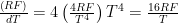
4RF = sT4 (4)
When eq. (4) is derived, it will be
d(RF)/dT = 4sT3 = 4RF/T (5)
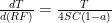
The ratio d(RF)/dT can be inverted transforming it to CSP
dT/d(RF) = CSP = T/(4RF) = T/(SC(1-a)) (6)
The average albedo value can be calculated from the observed reflected flux and the average solar irradiation values to be 104.2 W/m2 and 342 W/m2 = 0.30468. The temperature calculated by eq. (3) is
-18.7 degrees. According to Planck’s equation, this temperature corresponds to radiation flux of 237.8 W/m2 and it is also the observed flux value emitted by the Earth into space. Theory and practise are the same, when the theory is correct. According to eq. (6), CSP is 0.268 K/(W/m2).
There is a big difference between the CSP value of 0.5 K/(W/m2) and 0.268 K/(W/m2). The reason is well-known. The above calculations do not assume any changes in the absolute water content of the atmosphere. IPCC and the Global Climate Models (GCMs) assume a constant relative humidity (RH) in the atmosphere. It means that, when CO2 increases the global temperature and when the RH stays constant, the small increase of the absolute water content in the atmosphere increases the temperature. How much? IPCC writes in AR4 in section 8.6.3.1 that water vapor roughly doubles the response to forcing of GH gases and it is called positive waster feedback. In AR5 IPCC writes that water vapor’s contribution is approximately two to three times greater than that of CO2. I have checked that the doubling effect of water technically correct because water is about 12 times stronger a GH gas than CO2 in the present climate (ref. 6) but the question is if the RH is really constant in the atmosphere.
The observed RH values measured from 1948 to 2012 are depicted in Figure 1 and they and they show that RH values are not constant.

Figure 1. Relative Humidity graphs from 1948 to 2016.
It is obvious that the assumption of constant RH is not valid. Applying the CSP value of 0.268 K/(W/m2) and the RF value of 3.71 W/m2, the SC is 1.0 degrees, which is usually called Planck’s CS. As listed before, many researchers have applied different methods in calculating the CS value and a typical value is from 1.0 to 1.2 degrees. There is a good chance that these research studies have found this very same feature that there is no positive water feedback, which could double the RF value of 3.7 W/m2.
4. Radiative Forcing of carbon dioxide
IPCC uses the RF formula of Myhre et al. represented in eq. (2). The formulas of Hansen et al. (ref. 2) and Shi (ref. 3) give almost the same results as one can see in Figure 2. Eq. (2) of Myhre et al. is simple and easy to use. It is a kind of standard as a measure of CO2 warming effect and it is called even “and iconic formula”.

Figure 2. The RF values of CO2 according to Myhre et al., Hansen et al., Shi, and Ollila.
The first hint about the problems of this formula comes from the paper of Shi published in 1992 in journal by name “Science in China – Series B”. It is not available through network and I have received a personal electronic copy from the author himself. In Figure 3 is a print screen from a sentence, which states that the author has used a fixed RH value in his calculations. This means that the water has doubled the RF value of CO2.

Figure 3. The RH assumption of Shi.
The only way to find out the real RF relationship is to carry out the CS calculations according to the specification of CS (ref. 4). I have used the application Spectral Calculator available through Internet and this software uses Line-By-Line (LBL) method. A very essential thing is to use the Average Global Atmosphere (AGA) profile of the Earth for the temperature, pressure and humidity. I have combined the AGA profile from the five climate zones of the Earth (available in Spectral Calculator), which has the TPW (Total Precipitated Water) value of 2.6 cm and the surface temperature of 15.0 degrees.
First I have calculated the OLR (outgoing longwave radiation) at the TOA for the CO2 concentration of 280 ppm. The OLR is the sum of emitted radiation by the atmosphere 183.8 W/m2 and the transmittance (the portion of the surface emitted radiation not absorbed by the atmosphere) 81.6 W/m2, together 265.4 W/m2. When the CO2 is increased to 560 ppm, the same radiation values are: emission 183.4 Wm2 and transmittance 79.2 Wm2, together 262.7 W/m2. Now we can see the effects of increased absorption caused by the increased concentration of CO2; the OLR has decreased as it should happen according to the theory of GH effect. Because the Earth obeys the first law of energy conservation, the ORL must increase to the original value of 265.4 W/m2. The only way this can happen, is the higher surface temperature of the Earth. By trial and error, I have found that the temperature 15.66 degrees gives emission rate of 185.0 W/m2 and transmittance of 80.4 W/m2, together 265.4 W/m2.
Because the cloudy sky calculations are not possible in Spectral Calculator, I have calculated the clear and cloudy sky values by the MODTRAN application. These results show 30 % lower OLR change than the clear sky. IPCC reports that the reduction is 25 %. Using the MODTRAN figures, the result is that the TCS value is 0.56 degrees and CSP is 0.259 K/(W/m2). The CSP value is very close to the Planck’s CSP = 0.268 K/(W/m2).
The original study of mine is published in 2014 in Development of Earth Science by title “The potency of carbon dioxide (CO2) as a Greenhouse gas” (ref. 4). My formula for the RF of CO2 is
RF = 3.12 * ln(C/280) (7)
The warming values of CO2 according to eq. (7) is depicted also in Figure 2. It is about 50 % lower than the graph of Myhre et al. In Figure 2 is also depicted a modified curve of Myhre et al. and it is done by multiplying the values of the original formula by 0.5 for eliminating the assumed water effect. This curve is fairly close to the curve depicted by eq. (7).
My CS calculations according to its specification and the text of Shi shows that the RF value of CO2 calculated by eq. (2) of Myhre et al. can be explained, if the warming effects of water are included by assuming the constant atmospheric RH conditions. There is also another possible explanation for the eq. (2). Myhre et al. have used in calculations water vapor and temperature data from the European Centre for Medium-Range Weather Forecast. This data is not publicly available and it is impossible to check what is the average global TPW value of this data.
The conclusion is that the IPCC’s warming values are about 200 % too high (1.75 degrees versus 0.6 degrees) because both the CO2 radiative forcing equation, and the CS calculation include water feedback. It is well-known that IPCC uses the water feedback in doubling the GH gas effects; even though there are relative humidity measurements showing that this assumption is not justified. CO2 radiative forcing by Myhre et al. includes also water feedback, and this has not been recognized before the author’s studies. This feature explains too high of a contribution of CO2.
5. Validation of results
Firstly, I want to show that my spectral calculations are correct, if compared to some other published results. Kiehl & Trenbarth (ref. 6) have published in 2009 an article, in which is probably the most generally used Earth’s energy balance presentation. In the LBL spectral calculations they used U.S. Standard Atmosphere 76 atmospheric profiles. They reduced the absolute water amount TWP by 12 %. Using this atmosphere, they calculated that the warming contribution of CO2 in the clear sky is 26 %; Also, this results is probably the most referred figure about the strength of CO2 as a GH gas.
I have reproduced this calculation by using Spectral Calculator and my result is 27 % – close enough. There is only one small problem, because the water content of this atmosphere is really the atmosphere over the USA and not over the globe. The difference in the water content is great: 1.43 prcm versus 2.6 prcm. I have been really astonished about the reactions of the climate scientists about this fact. It looks like that they do not understand the effects of this choice or they do not care. Which alternative is worse? The real contribution of CO2 in using the right TWP value is 13 % (ref. 7 ).
My LBL spectral analysis is based always on the calculation of the total absorption, transmission or emission in the atmosphere. For example, the effects of GH gases are based on the variations of their concentrations. Stephens et al. (ref. 8) has summarized the results 13 of studies based on the observed values of the downward LW radiation by the atmosphere right on the surface of the Earth. The results vary from 309.2 to 326 W/m2 and the average value is 314.2 W/m2. My calculation gives the result of 310.9 W/m2, which differs 1 % from the average observed value and it is well inside the error margin of +/- 10 Wm2, which is estimated accuracy of measured LW fluxes.
References
1. Myhre, G., Highwood, E.J., Shine, K.P., and Stordal, F. 1998. “New estimates of radiative forcing due to well mixed greenhouse gases.” Geophys. Res. Lett. 25, 2715-2718. http://onlinelibrary.wiley.com/doi/10.1029/98GL01908/epdf
2. Hansen, J., Fung, I., Lacis, I., Rind, A., Lebedeff, D., Ruedy, S., Russell,G., and Stone, P. 1998. “Global Climate Changes as Forecast by Goddard Institute for Space Studies, Three Dimensional Model.” J. Geophys. Res., 93, 9341-9364. https://pubs.giss.nasa.gov/abs/ha02700w.html
3. Shi, G-Y. 1992. “Radiative forcing and greenhouse effect due to the atmospheric trace gases.” Science in China (Series B), 35, 217-229. Not available online.
4. Ollila, A. 2014. “The potency of carbon dioxide (CO2) as a greenhouse gas”. Dev. Earth Sc., 2, 20-30.
http://www.seipub.org/des/paperInfo.aspx?ID=17162
5. Kielh, J.T. and Trenbarth, K.E. 1997. “Earth’s Annual Global Mean Energy Budget.” Bull. Amer. Meteor. Soc. 90, 311-323. http://journals.ametsoc.org/doi/pdf/10.1175/1520-0477%281997%29078%3C0197%3AEAGMEB%3E2.0.CO%3B2
6. Ollila, A. 2017. “Warming effect reanalysis of greenhouse gases and clouds”. Ph. Sc. Int. J., 13, 1-13. http://www.sciencedomain.org/abstract/17484
7. Stephens, G.L., et al. 2012. “The global character of the flux of downward longwave radiation”. J. Clim., 25, 2329-2340. http://journals.ametsoc.org/doi/pdf/10.1175/JCLI-D-11-00262.1
A point I’ve made before is that the IPCC’s notion of a feedback is:
GHG > Warming > H2O (X2) > Warming.
The problem with this model, and where it differs from feedbacks in electronic or process control, is that the input and output of the water vapour ‘amplifier’ are the exact same point in the loop. They are directly connected together, so the amount of output fed back can never be anything but 100%.
If positive feedback were used in electronics, it would normally consist of feeding back a reduced portion of the output. Directly connecting the output to the input, means that the output cannot be any larger than the input to the amplification stage. Which would seem to be a problem since any feedback gain at all, even 1.000001x, let alone 2x, would then lead to instability.
It’s a bit like the ‘bootstrap’ arrangement sometimes used to reduce input loading in electronics. Such an arrangement must have less than unity gain though, or it will cause instability.
I’ve thought long and hard about how such a system could provide a measured amount of amplification without going unstable. I don’t see how it can. It could provide attenuation though.
I have myself an automation engineer and process engineer background. The positive feedback alone, would make any system unstable.
This hits me like a very strong argument. Similar to whenever someone lets a microphone pass in front of its connected amplifier and then starts to speak.
I would very much like to hear the counter argument to this.
There is none. I was an electronic and semiconductor designer and simulation expert for 14 years, positive feedback alone is always unstable. Always.
Their argument is, “Well, no one says it positive alone, it’s just positive in co2 water feedback” Which is not only wrong, it is a lie of omission, because there has to be an equal an opposite negative feed back or limit, other wise we would not be here to wonder about such things, and they always fail to mention that.
I’m an old retired CFO (numbers guy…), and what I get from this very interesting & helpful post is:
1) The science is not settled (Gosh, Al Gore lied to us…again)
2) The math is not even accurate
So, pray tell, how do the model results compare with the actual data?
If the models work, no difficulty at all should be encountered in replicating the historical climate; say starting at the onset of the the Medieval Warming Period, through the little Ice Age, up until, say, the year 1900 (before significant man made CO2 added another confounding variable to complicate modeling a chaotic system).
Of course, the models should faithfully replicate – and PREDICT !!! – the climate “switch” to the Little Ice Age from the MWP (this should be a breeze; after all the “answer is known.” )
Surely, the above is child’s play. After all, the AGW proponents have predicted the climate 100 years hence.
So, back-predicting should be a snap.
Here is a reminder, from a real scientist, Richard Feynman, regarding the KEY TO SCIENCE ;
https://youtu.be/b240PGCMwV0
Here are some comparisons of the IPCC model temperature values according to equations 1 and 2 compared with actual measured temperature. The error in the end of 2016 is about 50 %.

‘an ecumenical matter’ rather than a ‘canonical estimate’ I believe (in hono(u)r of St Patrick’s Day)!
Dr Ollila, I’m reading with great interest, have not finished, so I’m sure I will post more. My research confirms surface RH has declined, in part due to an increase in temp without a corresponding increase in dew point. Dew Points did shift with the rise in temps at the end of the 1999 El Nino, but that still left rel humidity falling.
Visible in this graph of 59 million surface station records.
But
This is fatally flawed. The cooling process is not a static process.
It actively changes during clear sky cooling, and an average single line by line run is like taking a single measurement in the middle of the day, worthless to look at the radiative process as temps fall and RH rises every night.
Here’s what the actual measurements look like
AS you can see there are two distinct cooling rates, and the change between them is based on air temps nearing dew point, and rel humidity increasing, once it’s over about 70 or 80%. With more data I suspect this percentage will be influenced on the absolute humidity.
I’ve also calculated the change temperature of every surface station outside of the tropic as the seasons change the length of day, and then I used measured tsi to calculate a clear sky surface forcing, which I divide the rate of temp change by to get a Delta degree F/ W/m-2
You can see these results by latitude bands here.
https://micro6500blog.wordpress.com/2016/05/18/measuring-surface-climate-sensitivity/
Wow micro an actual post! Now it’s worth taking time to look at your work.
BTW, just so you know. I figured I wouldn’t have to explain 3 lines on that graph to everyone. I though, at least with a few hints, and what I have written someone else would also figure it out. But so it goes…….
Finished. Okay, looks like a clear increase in temperature. Except the atm is nonlinear in cooling, and what you calculated was an average, like taking the average of the output going to a speaker, and not knowing all those squiggly lines were music, if you didn’t average it all away.
So, how the active process in the last graph above works out. Since on land, there isn’t a lot of readily available of water to evaporate, so dew points don’t change particularly fast, at least compared to how quickly the day changes conditions. So, say we have clear skies, calm conditions with a constant dew point of say 33F, and the switch between the 2 cooling rates is at ~90% ~47F and it switches between 4F/hr to 1F/hr (approximately what the measured data did)
So @ur momisugly 7:00pm ~72F
8:00=68F
9:00=64F
10:00=60F
11:00=56F
12:00=52F
1:00=48F
2:00= .25×4 + .75×1 = 1.75F, to avoid fractions I’ll round up to 2F so
2:00=46F
3:00=45F
4:00=44F
5:00=43F
6:00=42F
which is pretty close to the chart.
Now, let’s assume Co2 make this same day 4F warmer.
7:00=72F/76F
8:00=68F/72F
9:00=64F/68F
10:00=60F/64F
11:00=56F/60F
12:00=52F/56F
1:00=48F/52F
2:00=46F/48F
3:00=45F/47F
4:00=44F/46F
5:00=43F/45F
6:00=42F/44F
It reduced a 4F increase in max temp to 2F of warming. Also it does ultimately catch up (the rate does continue to slow) as summer turns to fall. This is Australian spring, and each day get a little longer, so there is less time to cool, where in the fall it catches up, hence it warms in the spring and cools in the fall.
Nonlinear cooling!
Reality check: It is nearly spring and here where I live in the NE it is often this last month, near or below zero F which is typical of a very cold JANUARY. It is going to be a high of 23 degrees F Monday and a low of 4 above zero F. This is insanely cold for this time of year, we are buried under two plus feet of snow, too.
So much for getting warmer and warmer.
Here’s an example of ~ 60 years of the change plotted out for the US.


Warming
Remember it’s the rate of change per day, and in October it’s dropping the most per day, in november it’s still dropping, only less so.
It is counter intuitive
Oh, the graphs are change per day in degree F * 100.
I live in Ohio, and while it is cold today, it was 80 last week?
I have tried to reproduce what Myhre et al. have done in calculating the RF effect of CO2 increase from 280 to 560 ppm. I think it is basically a correct procedure, because I can produce – as I have shown in the validation section – that the total absorption in the atmosphere is same as observed on the surface.
I clarify my comment above. The procedure of Myhre et al. is correct. The small concentration changes from the balance situation can be described with a simple logarithmic equation. The problem is that it seems to include positive waster feedback as written by Shi and therefore the result is not correct.
The low cooling rate is due to low surface temperature and the high cooling rate is due to high surface temperature. (Surface temperature leads the air temperature, which is measured 2 meters above the surface.) Notably, the amount of water vapor in the air is fairly constant throughout the day-night cycles shown in the graph. The first nighttime low looks like about 36 degrees F at close to 100% relative humidity, which means a dewpoint of 35-36 degrees F. The next daily high is about 69 degrees at about 38% relative humidity, which means a dewpoint about 40 degrees F.
“The low cooling rate is due to low surface temperature ” No, equilibrium isn’t reached. At least not until later still. It might look like that is the case, but the optical window remains still 80 to 100F colder than air temps, even during the low cooling rate. But my IR doesn’t get the water lines longer than 14u, and that should be very active that this time, and they likely light Co2 up in the process.
I did not claim anything requiring equilibrium to be reached. If it was reached during the night, then the cooling rate would drop to zero during the night.
Meanwhile, the optical window is not the only thing above the surface. There are also the greenhouse gases, which are mostly far less than 80-100 degrees C different in temperature than the surface, and which mostly have a much smaller temperature drop during the night than the surface does. Note the spread between high and low daily temperatures at the 500, 700 and even the 850 millibar levels – generally a fraction of the spread at 2 meters above the surface (except where the surface elevation gets close to one of these levels).
If they are not dropping at night they are not radiating, or all of the gas they are in is not radiating.
Here’s the paper that also found cooling rates were not completely explained.
What Determines the Nocturnal Cooling Timescale at 2 m
http://www.google.com/url?sa=t&source=web&cd=1&ved=0ahUKEwjjqcaGt8XQAhVD9YMKHZ0iCa4QFggaMAA&url=http%3A%2F%2Fonlinelibrary.wiley.com%2Fdoi%2F10.1029%2F2003GL019137%2Fpdf&usg=AFQjCNF8lW-CCS7EPxfpANvf5ZKO1PcNfQ
And that’s what I solved.
One thing the graph of daily temperature and radiation results shows is nighttime temperature leveling off even though heat is being lost by radiation. There is a common, simple cause of this when the relative humidity is high at 2m and 100% at the surface: Formation of dew. Latent heat is being released.
Yes, I agree. But the magic is that the transition between the 2 cooling rates is temperature dependent.
That is the action, is basically how switching power supply regulate voltage. The pulses of current flows, go to charge a capacitor, and the current pulses happen once a cycle, depending of the voltage at the time.
Surface temps do exactly the same, except on the outgoing current, this regulates the minimum level, instead of the maximum level.
Oh, one more note, dew starts forming about the time the rate slows, well before 100%.
Dew starts forming before the relative humidity at the standard measurement altitude of 2 meters is 100%. At that time, the surface is cooler than the air 2 meters above it.
Only if it’s covered in vegetation. Dirt, and many man made structures are still warm.
Vegetation coverage is not necessary for the surface to cool more quickly during nights than the air 2 meters above the surface. Such faster surface cooling is common in deserts, drought-affected farms, and snow-covered treeless rural areas. And, when the surface is covered with vegetation much taller than 2 meters such as trees, the surface and the air 2 meters above the surface track well in temperature. Bare uncovered dirt surface can cool faster during the night than the air 2 meters above it – the dirt is what is radiating heat away to outer space and cooling the air 2 meters above it, so the air 2 meters above the surface has its cooling temperature lagging the temperature of the surface during the night.
I don’t have dirt in my front yard, but I have measured a dirt colored brick patio and it cooled slower than air, and here’s grass, sky, concrete and asphalt, and the grass cools off quickly, concrete cools slowly, and asphalt slower still

And it’s still not equilibrium. Did you read this?
What Determines the Nocturnal Cooling Timescale at 2 m
http://www.google.com/url?sa=t&source=web&cd=1&ved=0ahUKEwjjqcaGt8XQAhVD9YMKHZ0iCa4QFggaMAA&url=http%3A%2F%2Fonlinelibrary.wiley.com%2Fdoi%2F10.1029%2F2003GL019137%2Fpdf&usg=AFQjCNF8lW-CCS7EPxfpANvf5ZKO1PcNfQ
You have a diverse surface. Some of it will cool faster, some of it will cool slower during the night. The cooling surface as a whole cools the air, even though the air can be cooled faster than the slowest-cooling surface materials.
Fine, as the paper I referenced mentions, that does not explain the measurements by themselves.
What I’ve added does. And it matches the emergent behavior of surface temperature as measured at 2 m, which is what all of us have been arguing about for far, far too long.
Actually not only the surface, but the same emergent behavior at TOA that Willis recently wrote about would evolve from this process.
What emergent behavior taking place late at night did Willis write about? Please cite. I have known emergent behavior to be written about as an afternoon event so as to be some sort of upper-limit thermostat for the surface temperature of tropical oceans.
Also, why can’t late night emergent behavior be dew (or frost if the dewpoint is below freezing)?
I have checked that the doubling effect of water technically correct because water is about 12 times stronger a GH gas than CO2
Really? And here I thought that CH4 (methane) is pound for pound 86 times as strong a GH gas as CO2. Don’t believe me? Just do a Google search on [Methane 86] and it will become abundantly clear, the media wouldn’t lie you know. So that means that methane is at least seven times as strong as water vapor.
OK that’s a bit off topic but the methane is a zillion times more powerful than CO2 meme that’s been bandied about for the last few years really needs to be explained in depth. The question, “How much will CH4 at ~1800 ppb and increasing at ~7 ppb every year actually run up the average temperature a century from now?” really needs to be answered.
I forgot to say that public policy is being decided on the basis of the 86 times more powerful misdirection.
The reason CH4 is so ‘powerful’ is because its both its concentration and current contribution are so low. CH4 affects only a tiny part of the LWIR spectrum, while CO2 and H2O affect far more wavelengths of photons. Once the CH4 lines start to saturate, the incremental effect will be far less than the incremental effect of CO2, H2O or even Ozone.
Well, the strengths of CH4 and N2O can be regarded very strong also, if their concentrations would grow to let say to 10 or 50 ppm but they will not and therefore they can be forgotten. In the previous figure of the absorption areas of GH gases this is shown very clearly, because the areas of the two GH gases is totally overlapping with the water.
Here is figure showing the temperature effects of GH gases. The red dots are the present concentrations

The reason CH4 is so ‘powerful’ is because….
No argument here, but let’s do a “Back of the envelope estimation” to see what’s going on:
To make things simple, let express CH4 in terms of parts per million instead of parts per billion, or about 2 ppm., then let’s double it by adding 2 ppm. and we get 4 ppm. Now let’s do the same for CO2. No we don’t double CO2 we add just 2 ppm CO2 and on top of that due to the pound for pound statement and the fact that MH4 is 36% the mass of CO2, we will be adding not 2 ppm but 36% of 2 ppm or 0.7 ppm. That comes an increase in CO2 from about 400 ppm to 400.7 ppm, or a 0.2% increase instead of the 100% increase for CH4. At this point it should be abundantly clear what’s going on here. And to then continue, 0.2% of CO2’s absolute climate sensitivity of about 1.2 K would be 0.002 K. If you then multiply that times 86 it comes to nearly 0.2 K.
If policy makers were to understand that at current rates it would take about 300 years to double CH4 and that it would result in perhaps a 0.2 K increase, then just maybe they wouldn’t get so excited. But 86 times more potent than CO2 is really quite the scary hobgoblin that the general populace needs to be rescued from isn’t it.
I’ve done some investigation as to what the “Climate Sensitivity” of CH4 is and I find estimates from 0.1 K to 0.3 K so 0.2 K for a doubling seems to be in the ball park.
The IPCC has now admitted that it doesn’t know what the climate sensitivity is.The IPCC AR4 SPM report section 8.6 deals with forcing, feedbacks and climate sensitivity. It recognizes the shortcomings of the models. Section 8.6.4 concludes in paragraph 4 (4): “Moreover it is not yet clear which tests are critical for constraining the future projections, consequently a set of model metrics that might be used to narrow the range of plausible climate change feedbacks and climate sensitivity has yet to be developed”
What could be clearer? The IPCC itself said in 2007 that it doesn’t even know what metrics to put into the models to test their reliability. That is, it doesn’t know what future temperatures will be and therefore can’t calculate the climate sensitivity to CO2. This also begs a further question of what erroneous assumptions (e.g., that CO2 is the main climate driver) went into the “plausible” models to be tested any way. The IPCC itself has now recognized this uncertainty in estimating CS – the AR5 SPM says in Footnote 16 page 16 (5): “No best estimate for equilibrium climate sensitivity can now be given because of a lack of agreement on values across assessed lines of evidence and studies.” Paradoxically the claim is still made that the UNFCCC Agenda 21 actions can dial up a desired temperature by controlling CO2 levels. This is cognitive dissonance so extreme as to be irrational. There is no empirical evidence which requires that anthropogenic CO2 has any significant effect on global temperatures. For a complete discussion see my recent paper from E&E at http://climatesense-norpag.blogspot.com/2017/02/the-coming-cooling-usefully-accurate_17.html
Here is the abstract for convenience.
ABSTRACT
This paper argues that the methods used by the establishment climate science community are not fit for purpose and that a new forecasting paradigm should be adopted. Earth’s climate is the result of resonances and beats between various quasi-cyclic processes of varying wavelengths. It is not possible to forecast the future unless we have a good understanding of where the earth is in time in relation to the current phases of those different interacting natural quasi periodicities. Evidence is presented specifying the timing and amplitude of the natural 60+/- year and, more importantly, 1,000 year periodicities (observed emergent behaviors) that are so obvious in the temperature record. Data related to the solar climate driver is discussed and the solar cycle 22 low in the neutron count (high solar activity) in 1991 is identified as a solar activity millennial peak and correlated with the millennial peak -inversion point – in the RSS temperature trend in about 2004. The cyclic trends are projected forward and predict a probable general temperature decline in the coming decades and centuries. Estimates of the timing and amplitude of the coming cooling are made. If the real climate outcomes follow a trend which approaches the near term forecasts of this working hypothesis, the divergence between the IPCC forecasts and those projected by this paper will be so large by 2021 as to make the current, supposedly actionable, level of confidence in the IPCC forecasts untenable.
As commented below, IPCC is playing with two cards. In the scientific section of AR5 IPCC tries to soften its scientific conclusions (a big gap between lower and higher limits of CS). On the other hand the Paris climate agreement is based on the IPCC*s model that doubling of CO2 concentration to 560 ppm will increase the global temperature over the 2 degrees and we need really hard measures to prevent this. The whole agreement is based on the IPCC*s science or do you know that there is some other scientific basis?
Does the IPCC say that
“…a doubling of CO2 will or does cause…”
or do they say that
“…a doubling of CO2 may or might cause…”?
Does the IPCC say that…
Doesn’t matter, the news media, Hollywood, Democrats and public school teachers say that CO2 is going to cause a catastrophic disaster.
I be one of those and I don’t say that. Neither do most of my colleagues here in NEOregon. Broad brushes are usually used by people who speak before they reason.
Pamela Gray March 17, 2017 at 9:14 am
I be one of those and I don’t say that.
Criticism accepted. How ’bout “many public schools” instead of “public school teachers”?
It would be pretty unscientific for the IPCC to talk in terms of certainty about ECS, or anything else for that matter. Rather it’s assessment is stated in the usual probabilistic scientific terms:
The terms ‘likely’, ‘extremely unlikely’, etc are all quantified in percentage terms. Using these the above quote can be paraphrased as follows:
For full explanation and further links download the AR5 SPM from here: http://www.ipcc.ch/report/ar5/wg1/
I understand DWR54.
However, my attempted point is that since the IPCC admits that the matter isn’t certain, then are they not admitting that the science isn’t settled?
I have high confidence that the IPCC is incorrect about everything they say!
The problem with climate science is that, as the late Dr. Joanne Simpson said, it is almost entirely based on computer models. And, the physics of CO2 & temperature goes only a part of the way needed for the models to fit the historical proxy data. So, what to do? Why, add a fudge factor in to the models, of course – that makes it quite easy to curve-fit the models to the data. But, of course, they cannot actually call it what it is – a fudge factor – so they called it a sensitivity factor.
So, can we then assume, since the physics of the CO2-water vapor link is not at all understood, all the rest of the physics is understood? Well, maybe not. If it was, wouldn’t there be *ONE* value for this fudge factor for all models? How can the physics, other than this one part, be understood and have a range of fudge factors from 1.5 to 4.5 degrees C, as Nick Stokes said?
Now, if anyone doubts this, simply ask anyone who wants to argue that the “science is settled” about what the science actually consists of that shows man made CO2 to be a significant part of any observed current warming. They most likely will not know. If they do know, they will not wish to talk about it. Ask them, if they either do not know, or they do not wish to discuss it, how they can base their argument on an obvious religious type belief rather than any knowledge of the actual science. There is no real technical knowledge needed to outline in general terms what the science consists of.
One more thing that is interesting. A person can find the answer to almost any question today using google search. I have asked this question time after time, and I know that people have gone to google to find the answer. Why is it that a question as easy to answer as this cannot be found in this way? Is it because the people who know do not wish to make it easy to understand?
My experience is in markets. My “hobby” (and also my living to a good extent) has been in building models to predict future price changes in selected markets (especially one that I know well). I’ve been enjoying working with this for well over tweny-five years. One of the things I have learned is that a model that is curve-fit to historical data is a model that will cost a person money. It has become obvious to me over the years that if climate scientists were dependent on their models being useful in real time for their livelihoods, the profession would have a lot fewer scientists.
Well now that their funding is going to dry up their going to find out.
Because we do not know all the causes for global warming, it is impossible to calculate from the observed temperature increase, what is the real climate sensitivity. But if the model used for calculation of CS, gives temperatures which is now about 50 % too high, then you can conclude that the model overestimate the contribution of CO2. My model for the CO2 warming does not explain totally the present temperature, but it leaves some room for unknown factors, see figure below.
Link to the original paper: http://www.sciencedomain.org/abstract/17484

One comment for the figure above.
There is an essential feature in the long-term trends of temperature and TPW, which are calculated and depicted as 11 years running mean values. The long-term value of temperature has increased about 0.4 ºC since 1979 and now it has paused to this level. The long-term trend of TPW shows minor decrease of 0.05 ºC during the temperature increasing period from 1979 to 2000 and thereafter only a small increase of 0.08 ºC during the present temperature pause period. It means that the absolute water amount of the atmosphere is practically constant reacting only very slightly to the long-term trends of temperature changes. Long-term changes, which last at least one solar cycle (from 10.5 to 13.5 years), are the shortest period to be analyzed in the climate change science. The assumption that the relative humidity is constant and it amplifies the GH gas changes by doubling the warming effects, finds no grounds based on the behavior of TWP trend.
NOAA/NASA define ToA as 100 km. 99% of the atmospheric mass is contained below 32 km. There are essentially no molecules between 32 km and 100 km. How does any of this work with zero molecules?
https://en.wikipedia.org/wiki/High-altitude_balloon
Below is a figure about the absorption in the atmosphere per altitude. The absorption in 1 km altitude is 90 % from the final altitude and in the altitude of 11 km (the upper limit of the troposphere) it is already 98 %. The GH phenomenon happens in the troposphere.

So if the incoming/outgoing radiative balance, ISR – albedo = ASR = 240 in and 17+80+63 +80 = 240 out, is at 100 km and CO2/GHGs do their thang below 11 km how do they have any measurable impact on the radiative balance at ToA of 100 km?
Answer: they don’t, nada, zip, zero.
https://www.linkedin.com/pulse/what-greenhouse-nicholas-schroeder
Mankind’s modelled additional atmospheric CO2 power flux (W/m^2, watt is power, energy over time) between 1750 and 2011, 261 years, is 2 W/m^2 of radiative forcing. (IPCC AR5 Fig SPM.5) Incoming solar RF is 340 W/m^2, albedo reflects 100 W/m^2 (+/- 30 & can’t be part of the 333), 160 W/m^2 reaches the surface (can’t be part of the 333), latent heat from the water cycle’s evaporation is 88 W/m2 (+/- 8). Mankind’s 2 W/m^2 contribution is obviously trivial, lost in the natural fluctuations.
One popular GHE theory power flux balance (“Atmospheric Moisture…. Trenberth et al 2011jcli24 Figure 10) has a spontaneous perpetual loop (333 W/m^2) flowing from cold to hot violating three fundamental thermodynamic laws. (1. Spontaneous energy out of nowhere, 2. perpetual loop w/o work, 3. cold to hot w/o work, 4. doesn’t matter because what’s in the system stays in the system)
Physics must be optional for “climate” science.
It’s lost during the non linear clear sky cooling cycle, I explain it in this thread somewhere.
Nicholas Schroeder. This comment comes out many times that the atmosphere emits more LW radiation downwards than the Earth’s surface emits upwards. It is not so. If you look at my energy balance figure below, you will see that the atmosphere emits downwards 344.7 W/m2 and the Earth emits 395.6 W/m2. There is no conflict with the physical laws.
When I look at Roy Spencer’s plot of model results vs. satellite and weather balloon data, I often ask what makes virtually all of the computer models so far off and why don’t they fix it? What is making their temp curves so bad? The simple answer, of course, is ‘garbage in, garbage out.’ Is it the assumed water vapor factor? All of the water vapor curves I’ve seen show water vapor decreasing since 1947 so how can the modelers assert that as CO2 rises, water vapor also rises and that is what raises the temp? When I ask computer modelers how much can increased CO2 raise temp without using a water vapor factor, I can’t get an answer.
When I look at strong temp fluctuations in past geologic time, only about 0.1% of warming periods have anything at all to do with CO2. When I look at the increase in CO2 levels after 1945, I find that the atmospheric content of CO2 has risen only 0.008% and this miniscule amount is supposed to warm 300 million cubic miles of ocean water? Add to this the fact that CO2 always lags temp, both long-term and short-term and you can see why I’m skeptical that CO2 has any significant effect on climate at all.
What is making their temp curves so bad?
My guess is because they are hind casting to adjusted temps….past cooled, present warmed
…which doesn’t match real time temps
and feedbacks are cancelling each other out….so they end up with linear is all they can do
If you look at my figure above about the temperature trend and the effects of CO2 from 1970 onward and the absolute water, some important conclusions can be drawn. The temperature has increased according to UAH, which is the most reliable measurement and so Is also the temperature effect of CO2. But the average value of water has been slightly going downwards. So water feedback increasing the CO2 warming has not been in place. This is another evidence that there is no positive water feedback, because the average water content has been almost constant and not increasing ´with the increasing concentration of CO2, which is a basic assumption of IPCC model and all computer models.
What is making their temp curves so bad?
Money
Everything went so well with the IPCC model up to year 2000. Then the temperature pause emerged. The models of IPCC as well as the GCMs are based on the use of positive water feedback. The essential content of my story here is that positive water feedback is not only in the CSP, it is also in the equation of Myhre et al. These models use positive water feedback twice and therefore the TCS sensitivity is three times to great and the ECS is six times too great. If IPCC would admit that this is the case, also the GCMs would collapse. As far as I know, there is not a single GCM utilising LBL spectral calculation in their model but they apply the results of Myhre et al. That is why the results are almost the same.
I haven’t seen a detailed analysis, but I suspect that the ‘everything was going well until 2000’ is due in large part to the corruption of the USHCN data by Hansen’s GISS.
When you can surf the Urban Heat Island effect while growth surrounds former pristine sites and fail to acknowledge it (or max it out at 0.15 deg C) you can show lots of temp growth…. but once you’ve used that up, then you have to deal with real atmospheric phenomena.
To Jim Hodgen. The issue of the global temperature measurements is another issue. I do rely on the UAH MSU measurements but not on the other data sets. In the newer updates of GISS/NASA/NCEI data sets, the history is getting colder and the data near the present day is getting warmer. The science behind the calculation of the global average temperatures cannot be that complicated. Nowadays we have alarming information what Dr. Karl did in preparation of the latest update for GISS.
What I do hope that there were a detailed analysis what is going on in this data tampering. There is already an request by Lamar Smith from the House of Representatives on this issue.
@ur momisugly Don Easterbrook March 17, 2017 at 8:05 am : A team of honest Atmospheric Physicists is needed to sort all this for the new US admin. They are the ones to ask, I reckon. Please use your influence with the new bosses…..
I have seen both 4W/m2 and 2W/m2 cited as radiative forcing for a doubling of CO2, with some stating that this can be measured. Is 4W/m2 the clear sky value and 2.2 the cloudy sky model per Myhre? In any case, what is the assumption for water vapor content? or are those values for dry air? If dry air, what is the “average” water vapor content of air in the tropics? it must be pretty high? Doubling CO2 may have negligible effect in a humid environment. So CO2 would have a larger effect in the mid-latitudes?
If you look at my series of posts in this thread, you’ll see a ~two state cooling at night under clear calm skies. I have also calculated enthalpy at min and max for every surface station in my ncdc dataset. The tropics have the highest energy, but have a slightly less than average drop in enthalpy, Deserts have half the total energy, but drop twice as much. That is the effect of water. Now back to my posts, tropics would likely spend more time in the low rate, and deserts are spending more time in the high state, and it like has to due with the rate of change in to 70 to 80% rel humidity range and above.
You can find the raw data with enthalpy here http://sourceforge.net/projects/gsod-rpts/
The whole problem of the CS value would have solved, if the CS could be measured. The right RF value for the all-sky (66 % clouds) is 3.71 W/m2 according to Myhre et al. The value of water content is the key. Based on my reproduction I conclude that I can get almost the same RF 3.71 W/m2, if I assume that the relative humidity is constant, which means that water doubles the RF value of CO2.
The OLR varies a lot over the different climate zones.
Here is figure about the absorption areas of GH gases and especially of CO2. Note the overlapping of absorption areas.

Here is the same in the tropic. The absorption area of CO2 is very small meaning very small warming effect. The whole GH effect is mainly due to the water.

Now calculate the absorption of just the anthropogenic fraction of CO2 and determine if that fraction is capable of changing weather pattern variations sufficiently to cause an increase in global temperature. But first you must calculate the energy needed to change weather pattern regimes from one stable state to a warmer one.
It can not be in static balance, as the surface of the 2 hemisphere’s are different, just picture how surface temps are distributed, plus you have energy getting stored away from the surface as well as stored energy moving from one place to another.
An annual average would be close, but even that doesn’t account for the AMO and PDO cycles.
Hi, since you are posting absorption gases. Why SO2 is not listed in the graph?
thanks.
In equation 5, I assume the last = sign is a result of solving equation 4 for s and substituting in for s in equation 5. If so, I think there is a constant issue as there will be a 4 picked up by substitution. I hope I did the LaTeX right.
substituting for s as above yields
This has implications for equation 6 in that there would now be a factor of 4 in the denominator.
The problem here of course is it then gives a value for CSP of 0.067230 which is even worse than what you started with. If someone can see where I went off course here let me know, but when someone does a derivation, I always try to reproduce it as I don’t trust anyone (including and especially myself) to do algebra correctly the first time through.
Darn! I left all the d’s off the derivatives in the numerators!
and
and typed a 4 where I needed a 3 on the exponent of the derivative…Man I really bombed that algebra test
The sensitivity is most accurately quantified as (4*o*e*T^3)^-1, where o is the SB constant and e is the ratio between the LWIR leaving the top of the atmosphere (239 W/m^2) and the LWIR leaving the surface at its average temperature of T (390 W/m^2 @ur momisugly 288K). What the IPCC neglects is the 1/T^3 dependence of the sensitivity on the temperature. They assume that the sensitivity at the poles is the same as it is at the equator which is absolutely incorrect given the T^4 dependence of emissions on temperature.
The only physical constant that relates temperature to emissions is the SB constant of 5.67E-8 W/m^2 per K^4. In AR1 and subsequent reports, the non linearity is mentioned but said to be approximately linear. While this is true, it’s only approximately linear over a very small range of temperatures and is far from linear across the range of temperatures exhibited by the planet. In their haste to support CAGW, they linearized the sensitivity as a slope passing through zero, rather than a slope based on the T^4 relationship. Note that the constant ‘e’ (effective emissivity) can be infinitely small and the T^4 relationship still persists.
This value for the sensitivity can be derived from first principles, measured easily and is highly repeatable. The sticking point is many refuse to accept that the planets behaves like a gray body. The objection is that “it must be more complicated than this”. Indeed how this behavior is manifested is complex, but the fact is that it the planet unambiguously manifests gray body behavior as shown in figure 3 in the following post. Also shown is the linearization error resulting in the absurdly high sensitivity claimed by the IPCC.
https://wattsupwiththat.com/2017/01/05/physical-constraints-on-the-climate-sensitivity/
To repeat this experiment, plot the average surface temperature against the average outgoing emissions for different parts of the planet (in this case, 2.5 degree slices of latitude) and the SB relationship will emerge every time, the slope of which represents the sensitivity of output emissions to temperature and since input power == output emissions, this is a fair proxy for the climate sensitivity. If you plot the average surface temperature vs. input power, the measured sensitivity is even lower approaching the sensitivity of an ideal BB at the surface temperature (4*o*T^3)^-1. Convergence to ideal behavior can be explained as the many degrees of freedom (complexity) self organizes to minimize the change in entropy upon state (surface temperature) changes. This is a basic requirement of the second law also called the entropy minimization principle.
My understanding is that the argument says an initial increase in C02 creates both warming (~1.0C for each doubling, although this declines each doubling) and water vapor, and that the water vapor creates the positive feedback loop by generating more warming (which generates more water vapor and so forth). This should be a runaway system (with feedbacks generating 50-80% or more of the warming depending on the sensitivity chosen), but the model outputs don’t look much like that. Is this because of lags built into the feedback equations or some dampening assumption? Just trying to understand how the feedback is handled.
Dan Tauke. IPCC do not use the real feedback mechanism. They just double the GH gas radiative forcing because of positive water feedback. They never did any system simulation including the real feedback in order to find the system response.
Regarding: “The calculation of the equilibrium CS (ECS) by IPCC applies positive feedbacks, which are not observed so far and are therefore very theoretical”:
This is not the distinction of equilibrium climate sensitivity from transient climate response.
TCS is the response during a 70 year period of CO2 doubling in a manner of exponential growth, which is a growth rate close to 1% per year. TCS includes some but not all of the effects of any feedbacks. ECS is the response after any feedbacks have completely run their course and the temperature of the ocean’s thermal mass has fully responded to the CO2 change.
TCS figures of 1.75, 1.85 or 2.5 degrees C per 2xCO2 include some positive feedback. With no feedbacks from change of cloud cover, water vapor, tendency of convection to occur, snow and ice coverage, etc. the ECS would be about 1.1 degrees C per 2xCO2 and the TCS even less.
Donald L. Klipstein. You writ. “TCS figures of 1.75, 1.85 or 2.5 degrees C per 2xCO2 include some positive feedback”. If you mean that it includes water feedback, this statement is correct. IPCC assumes that the positive water feedback in the atmosphere happens very quickly – not with the delays of years.
As I said, TCR (transient climate sensitivity) refers to a specific defined “transient” event whose duration is 70 years. I may be a little wrong here, it could be only 20 years – the Wikipedia article on climate sensitivity says that transient climate response is how climate responds to a 20 year period of CO2 increasing 1% per year. The calculated effect of such a “20-year transient” (my words) would have to be translated to terms of degrees C per doubling of CO2, using a formula where the effect of changing CO2 is logarithmic. 20 years is enough time for a change in snow and ice cover as well as water vapor concentration change from warming of the ocean surface, wetlands, ponds, puddles, and moist soils. The main lagging factor here is warming of the top few hundred meters of the ocean or maybe the “upper ocean” (the ocean above the thermocline).
Reproducible in isolation, with models, or in the wild? There is a predilection by [political] scientists to extrapolate from the first (in both time and space), indulge in circular reasoning with the second, and avoid the last with extreme prejudice.
Antero,
You said, “The average albedo value can be calculated from the observed reflected flux…” If the observation position is something like a geosynchronous weather satellite, then the apparent reflectivity (albedo) will be low because more than 70% of the surface of the Earth is capable of specular reflections of amounts greater than the nominal (lower-bound) 30% global albedo. The light reflected obliquely from water will go off into space in a direction not directly observable by a satellite, nor inferred from lunar estimates of Earth albedo. Additionally, light scattered from diffuse reflectors, such as clouds, will similarly leave in directions not observable by a nadir-viewing imaging satellite. The total reflectivity has to be obtained by modeling, based on satellite observations and theory. Unfortunately, obtaining reliable measurements from satellites, essentially looking into the sun, are fraught with difficulties including building a system with sufficient dynamic range and spatial resolution to capture the rapid change in reflectivity with high angles of incidence, as predicted by Fresnel’s Equation of reflection. This issue of “reflected flux” is just another issue of assumptions being made about the correct value of something only poorly measured.
It is beyond my expertise, if we talk about the technical problems with measuring the LW radiation emitted by Earth’s surface and detected by satellites. For the time being I rely on these observations, because I can close the Earth’s energy budget by using the observed radiation fluxes and some fluxes like absorption by GH gases calculated by LBL methods. I can even compare my theoretical LBL calculations with the observed reradiation flux at the surface.

This model treats the earth as a ball immersed in a bucket of warm fluid. Not even close to how it actually heats and cools.
Trenberth et al 2011jcli24 Figure 10
This popular balance graphic and assorted variations are based on a power flux, W/m^2. A W is not energy, but energy over time, i.e. 3.4 Btu/eng h or 3.6 kJ/SI h. The 342 W/m^2 ISR is determined by spreading the average 1,368 W/m^2 solar irradiance/constant over the spherical ToA surface area. (1,368/4 =342) There is no consideration of the elliptical orbit (perihelion = 1,416 W/m^2 to aphelion = 1,323 W/m^2) or day or night or seasons or tropospheric thickness or energy diffusion due to oblique incidence, etc. This popular balance models the earth as a ball suspended in a hot fluid with heat/energy/power entering evenly over the entire ToA spherical surface. This is not even close to how the real earth energy balance works. Everybody uses it. Everybody should know better.
An example of a real heat balance based on Btu/h follows. Basically (Incoming Solar Radiation spread over the earth’s cross sectional area), Btu/h = (U*A*dT et. al. leaving the lit side perpendicular to the spherical surface ToA), Btu/h + (U*A*dT et. al. leaving the dark side perpendicular to spherical surface area ToA), Btu/h.
The atmosphere is just a simple HVAC/heat flow/balance/insulation problem. Like Venus.
Mark Twain observed, “The trouble with most of us is that we know too much that ain’t so.”
https://www.linkedin.com/pulse/33c-nicholas-schroeder
Adding to the “Δ33C without an atmosphere” (see attached) that completely ain’t so is the example of Venus.
Venus, we are told, has an atmosphere that is almost pure carbon dioxide and an extremely high surface temperature, 750 K, and this is allegedly due to the radiative greenhouse effect, RGHE. But the only apparent defense is, “Well, WHAT else could it BE?!”
Well, what follows is the else it could be.
Venus is half the distance to the sun so its average solar constant/irradiance is twice as intense as that of earth, 2,615 W/m^2 as opposed to 1,368 W/m^2.
But the albedo of Venus is 0.77 compared to 0.31 for the Earth or Venus 601.5 net ASR (absorbed solar radiation) W/m^2 compared to Earth 943.9 net ASR W/m^2.
The Venusian atmosphere is 250 km thick as opposed to Earth at 100 km. Picture how hot you would get stacking 2.5 more blankets on your bed. RGHE’s got jack to do with it, it’s all Q = U A dT.
The thermal conductivity of carbon dioxide is about half that of air, 0.0146 W/m-K as opposed to 0.0240 W/m-K so it takes twice the dT/m to move the same kJ from surface to ToA (top of atmosphere, 100 km, 62 miles).
Put the higher irradiance & albedo (lower Q = lower dT), thickness (greater thickness increases dT) and conductivity (lower conductivity raises dT) all together: 601.5/943.9 * 250/100 * 0.0240/0.0146 = 2.61.
So, Q = U A dT suggests that the Venusian dT would be 2.61 times greater than that of Earth. If the surface of the Earth is 15C/288K and ToA is effectively 0K then Earth dT = 288K. Venus dT would be 2.61 * 288 K = 748.8 K surface temperature. No S-B BB RGHE hokey pokey need apply.
Simplest explanation for the observation.
Antero,
You said, “…but the question is if the RH is really constant in the atmosphere.” It seems to me that the absolute humidity should be used instead of the relative humidity.
Clyde. That is also my conclusion. Therefore I have used in my models and calculations the constant absolute amount of water – it is the constant TPW value of 2.6 cm.
I haven’t seen a grant application or award in 40 years. Do the current terms of government awards still come with the explicit stipulation that all data, methods and results must be made available for reproduction to anyone seeking that information?
I was wondering how much impact on reproducibility the ‘climate gangs’ penchant for withholding one or more of the above components has had on the field?
Regarding: “There is only one small problem, because the water content of this atmosphere is really the atmosphere over the USA and not over the globe. The difference in the water content is great: 1.43 prcm versus 2.6 prcm”:
Like CO2, water vapor’s effect is closer to logarithmic than linear. Correcting for the difference between 1.43 and 2.6 prcm makes only a minor change in the percentage of greenhouse gas effect contribution by CO2.
Donald. That is not so. The warming effects of water is practically linear over the large concentration range. You can find this feature in a figure “Temperature effects of GH gases”. That is why the water is so powerful GH gas, because it does not behave in the same way as the other GH gases. I copy below the absorption (=warming effects) of all major GH gases, if their concentrations have been increased by 10 % from the present concentration.
The increased absorption caused by the 10 % increase of concentration in AGA15 (average global atmosphere in 2015) atmosphere. The reference value of the AGA15 absorption is 310.69 Wm-2. The CO2 change* is based in the altitude of 1 km, because thereafter the absorption of CO2 does not increase.
GH gas Total absorption Absorption change Relative strength
H2O 315.129 4.439 11.765
CO2 310.996 0.394* 1
O3 310.998 0.308 0.782
N2O 310.745 0.055 0.140
CH4 310.733 0.043 0.109
Please not that the in the last column the strength of CO2 is 1 and therefore the relative strengths of other GH gases are relative to that of CO2. If you say that CH4 (Methane) or N2O (nitrogen oxide) are very strong GH gases, here you can see the real situation. The Global Warming Potential (GPW) values are totally artificial created to frightening people.
H2O increasing 10% causes increase from 310.69 to 315.129, by 4.439 W/m^2. And is not H2O vapor causing a majority of that 310.69 W/m^2? I don’t hear much of anyone claiming less than 65%, except when clouds are counted as greenhouse gases. 65% of 310.69 W/m^2 is 281.59 W/m^2.
Notably, Skeptical Science claims that water vapor contributes 75 W/m^2, and I think this is in a cloud-excluding breakdown cherrypicked to maximize calculated percentage of greenhouse gas warming being from CO2.
A 4.439 W/m^2 increase from 75-281.59 W/m^2 due to a 10% increase of water vapor is a 1.58-5.9 % increase in its effect as a greenhouse gas. Nowhere near linearly proportional. At this point I see SKS supporting 5.9% and aveollila supporting 1.58% increase of the warming effect of water vapor if it increases 10%. I can’t cite from this point that the effect of water wapor is as logarithmic as that of CO2, although it’s much less than linearly proportional.
Clouds have a very small effect in the total GH phenomenon and it is only 1%. The contributions of the GH gases are in percentages: water 81, CO2 13, O3 4, CH4 & N2O 1. In the total GH effect the strengths of H2O versus CO2 is 6.2/1 but in the present climate this relationship is 11.8/1.
Your Ref. 7 says in its abstract that total DLR is 344-350 W/m^2 plus or minus a possible error of 10 W/m^2, and clouds are responsible for 24-34 W/m^2 of that.
I noticed in your Ref. 6 that where you said the total is 310.69 W/m^2, you determined the effect of CO2 using 1 km, while you used 120 km for all other mentioned greenhouse gases. Not all of the absorption of CO2 can be accounted for from the lowest 1 km (about 10% of the atmosphere’s CO2).
Donald. Firstly about the energy balance fluxes. I refer now only to the presentation of mine. The clouds have a great effect on downward flux by the atmosphere: clear sky 318, and the cloudy sky 359 W/m2, difference 41 W/m2. The reason is that the clouds absorb totally the upward emitted flux by the surface – a complete GH effect.
The effects of clouds in calculating the contributions of GH gases in the GH effect is much more complicated. The first reason is that the clouds absorbs all the upward LW rAadiation but ast the same time they also reduce the incoming solar radiation. Both effects must be calculated.
I have calculated this many times and the situation is that the absolute absorption by CO2 does not increase above the altitude of 1 km. The relative contribution of CO2 even slightly decreases because the total absorption still increases thanks to water and to ozone in the stratosphere. It does not help at all that the CO2 concentration is almost the same up to 80 km. I would say that CO2 is a victim of its strength in the wave range from 12 to 16 micrometer. When there is no more radiation to be absorbed, then CO2 cannot absorb more. It is simple like that. Water has a very large absorption zone and that is one reason for its strength.
I have seen enough spectral absorption curves of the atmosphere, including one shown in comments above with the name Antero Ollila on it, where there are some wavelengths at which the whole atmosphere and the CO2 in it alone are partially transparent. This means that changing the CO2 concentration at any altitude at which CO2 exists would change the absorption spectrum. I would like to see how this can be reconciled with calculations that show no absorption on the way up by CO2 above 1 km.
Sorry, the World Press changed the outcome. If you look at the last values in each row, you will see the relative strengths.