Physical Constraints on the Climate Sensitivity

Guest essay by George White

For matter that’s absorbing and emitting energy, the emissions consequential to its temperature can be calculated exactly using the Stefan-Boltzmann Law,

1) P = εσT4

where P is the emissions in W/m2, T is the temperature of the emitting matter in degrees Kelvin, σ is the Stefan-Boltzmann constant whose value is about 5.67E-8 W/m2 per K4 and ε is the emissivity which is 1 for an ideal black body radiator and somewhere between 0 and 1 for a non ideal system also called a gray body. Wikipedia defines a Stefan-Boltzmann gray body as one “that does not absorb all incident radiation” although it doesn’t specify what happens to the unabsorbed energy which must either be reflected, passed through or do work other than heating the matter. This is a myopic view since the Stefan-Boltzmann Law is equally valid for quantifying a generalized gray body radiator whose source temperature is T and whose emissions are attenuated by an equivalent emissivity.

To conceptualize a gray body radiator, refer to Figure 1 which shows an ideal black body radiator whose emissions pass through a gray body filter where the emissions of the system are observed at the output of the filter. If T is the temperature of the black body, it’s also the temperature of the input to the gray body, thus Equation 1 still applies per Wikipedia’s over-constrained definition of a gray body. The emissivity then becomes the ratio between the energy flux on either side of the gray body filter. To be consistent with the Wikipedia definition, the path of the energy not being absorbed is omitted.

clip_image002

A key result is that for a system of radiating matter whose sole source of energy is that stored as its temperature, the only possible way to affect the relationship between its temperature and emissions is by varying ε since the exponent in T4 and σ are properties of immutable first principles physics and ε is the only free variable.

The units of emissions are Watt/meter2 and one Watt is one Joule per second. The climate system is linear to Joules meaning that if 1 Joule of photons arrives, 1 Joule of photons must leave and that each Joule of input contributes equally to the work done to sustain the average temperature independent of the frequency of the photons carrying that energy. This property of superposition in the energy domain is an important, unavoidable consequence of Conservation of Energy and often ignored.

The steady state condition for matter that’s both absorbing and emitting energy is that it must be receiving enough input energy to offset the emissions consequential to its temperature. If more arrives than is emitted, the temperature increases until the two are in balance. If less arrives, the temperature decreases until the input and output are again balanced. If the input goes to zero, T will decay to zero.

Since 1 calorie (4.18 Joules) increases the temperature of 1 gram of water by 1C, temperature is a linear metric of stored energy, however; owing to the T4 dependence of emissions, it’s a very non linear metric of radiated energy so while each degree of warmth requires the same incremental amount of stored energy, it requires an exponentially increasing incoming energy flux to keep from cooling.

The equilibrium climate sensitivity factor (hereafter called the sensitivity) is defined by the IPCC as the long term incremental increase in T given a 1 W/m2 increase in input, where incremental input is called forcing. This can be calculated for emitting matter in LTE by differentiating the Stefan-Boltzmann Law with respect to T and inverting the result. The value of dT/dP has the required units of degrees K per W/m2 and is the slope of the Stefan-Boltzmann relationship as a function of temperature given as,

2) dT/dP = (4εσT3)-1


A black body is nearly an exact model for the Moon. If P is the average energy flux density received from the Sun after reflection, the average temperature, T, and the sensitivity, dT/dP can be calculated exactly. If regions of the surface are analyzed independently, the average T and sensitivity for each region can be precisely determined. Due to the non linearity, it’s incorrect to sum up and average all the T’s for each region of the surface, but the power emitted by each region can be summed, averaged and converted into an equivalent average temperature by applying the Stefan-Boltzmann Law in reverse. Knowing the heat capacity per m2 of the surface, the dynamic response of the surface to the rising and setting Sun can also be calculated all of which was confirmed by equipment delivered to the Moon decades ago and more recently by the Lunar Reconnaissance Orbiter. Since the lunar surface in equilibrium with the Sun emits 1 W/m2 of emissions per W/m2 of power it receives, its surface power gain is 1.0. In an analytical sense, the surface power gain and surface sensitivity quantify the same thing, except for the units, where the power gain is dimensionless and independent of temperature, while the sensitivity as defined by the IPCC has a T-3 dependency and which is incorrectly considered to be approximately temperature independent.

A gray body emitter is one where the power emitted is less than would be expected for a black body at the same temperature. This is the only possibility since the emissivity can’t be greater than 1 without a source of power beyond the energy stored by the heated matter. The only place for the thermal energy to go, if not emitted, is back to the source and it’s this return of energy that manifests a temperature greater than the observable emissions suggest. The attenuation in output emissions may be spectrally uniform, spectrally specific or a combination of both and the equivalent emissivity is a scalar coefficient that embodies all possible attenuation components. Figure 2 illustrates how this is applied to Earth, where A represents the fraction of surface emissions absorbed by the atmosphere, (1 – A) is the fraction that passes through and the geometrical considerations for the difference between the area across which power is received by the atmosphere and the area across which power is emitted are accounted for. This leads to an emissivity for the gray body atmosphere of A and an effective emissivity for the system of (1 – A/2).

clip_image004

The average temperature of the Earth’s emitting surface at the bottom of the atmosphere is about 287K, has an emissivity very close to 1 and emits about 385 W/m2 per Equation 1. After accounting for reflection by the surface and clouds, the Earth receives about 240 W/m2 from the Sun, thus each W/m2 of input contributes equally to produce 1.6 W/m2 of surface emissions for a surface power gain of 1.6.

Two influences turn 240 W/m2 of solar input into 385 W/m2 of surface output. First is the effect of GHG’s which provides spectrally specific attenuation and second is the effect of the water in clouds which provides spectrally uniform attenuation. Both warm the surface by absorbing some fraction of surface emissions and after some delay, recycling about half of the energy back to the surface. Clouds also manifest a conditional cooling effect by increasing reflection unless the surface is covered in ice and snow when increasing clouds have only a warming influence.

Consider that if 290 W/m2 of the 385 W/m2 emitted by the surface is absorbed by atmospheric GHG’s and clouds (A ~ 0.75), the remaining 95 W/m2 passes directly into space. Atmospheric GHG’s and clouds absorb energy from the surface, while geometric considerations require the atmosphere to emit energy out to space and back to the surface in roughly equal proportions. Half of 290 W/m2 is 145 W/m2 which when added to the 95 W/m2 passed through the atmosphere exactly offsets the 240 W/m2 arriving from the Sun. When the remaining 145 W/m2 is added to the 240 W/m2 coming from the Sun, the total is 385 W/m2 exactly offsetting the 385 W/m2 emitted by the surface. If the atmosphere absorbed more than 290 W/m2, more than half of the absorbed energy would need to exit to space while less than half will be returned to the surface. If the atmosphere absorbed less, more than half must be returned to the surface and less would be sent into space. Given the geometric considerations of a gray body atmosphere and the measured effective emissivity of the system, the testable average fraction of surface emissions absorbed, A, can be predicted as,

3) A = 2(1 – ε)

Non radiant energy entering and leaving the atmosphere is not explicitly accounted for by the analysis, nor should it be, since only radiant energy transported by photons is relevant to the radiant balance and the corresponding sensitivity. Energy transported by matter includes convection and latent heat where the matter transporting energy can only be returned to the surface, primarily by weather. Whatever influences these have on the system are already accounted for by the LTE surface temperatures, thus their associated energies have a zero sum influence on the surface radiant emissions corresponding to its average temperature. Trenberth’s energy balance lumps the return of non radiant energy as part of the ‘back radiation’ term, which is technically incorrect since energy transported by matter is not radiation. To the extent that latent heat energy entering the atmosphere is radiated by clouds, less of the surface emissions absorbed by clouds must be emitted for balance. In LTE, clouds are both absorbing and emitting energy in equal amounts, thus any latent heat emitted into space is transient and will be offset by more surface energy being absorbed by atmospheric water.

The Earth can be accurately modeled as a black body surface with a gray body atmosphere, whose combination is a gray body emitter whose temperature is that of the surface and whose emissions are that of the planet. To complete the model, the required emissivity is about 0.62 which is the reciprocal of the surface power gain of 1.6 discussed earlier. Note that both values are dimensionless ratios with units of W/m2 per W/m2. Figure 3 demonstrates the predictive power of the simplest gray body model of the planet relative to satellite data.

Figure 3

climate-sensitivity-comparison

Each little red dot is the average monthly emissions of the planet plotted against the average monthly surface temperature for each 2.5 degree slice of latitude. The larger dots are the averages for each slice across 3 decades of measurements. The data comes from the ISCCP cloud data set provided by GISS, although the output power had to be reconstructed from radiative transfer model driven by surface and cloud temperatures, cloud opacity and GHG concentrations, all of which were supplied variables. The green line is the Stefan-Boltzmann gray body model with an emissivity of 0.62 plotted to the same scale as the data. Even when compared against short term monthly averages, the data closely corresponds to the model. An even closer match to the data arises when the minor second order dependencies of the emissivity on temperature are accounted for,. The biggest of these is a small decrease in emissivity as temperatures increase above about 273K (0C). This is the result of water vapor becoming important and the lack of surface ice above 0C. Modifying the effective emissivity is exactly what changing CO2 concentrations would do, except to a much lesser extent, and the 3.7 W/m2 of forcing said to arise from doubling CO2 is the solar forcing equivalent to a slight decrease in emissivity keeping solar forcing constant.

Near the equator, the emissivity increases with temperature in one hemisphere with an offsetting decrease in the other. The origin of this is uncertain but it may be an anomaly that has to do with the normalization applied to use 1 AU solar data which can also explain some other minor anomalous differences seen between hemispheres in the ISCCP data, but that otherwise average out globally.

When calculating sensitivities using Equation 2, the result for the gray body model of the Earth is about 0.3K per W/m2 while that for an ideal black body (ε = 1) at the surface temperature would be about 0.19K per W/m2, both of which are illustrated in Figure 3. Modeling the planet as an ideal black body emitting 240 W/m2 results in an equivalent temperature of 255K and a sensitivity of about 0.27K per W/m2 which is the slope of the black curve and slightly less than the equivalent gray body sensitivity represented as a green line on the black curve.

This establishes theoretical possibilities for the planet’s sensitivity somewhere between 0.19K and 0.3K per W/m2 for a thermodynamic model of the planet that conforms to the requirements of the Stefan-Boltzmann Law. It’s important to recognize that the Stefan-Boltzmann Law is an uncontroversial and immutable law of physics, derivable from first principles, quantifies how matter emits energy, has been settled science for more than a century and has been experimentally validated innumerable times.

A problem arises with the stated sensitivity of 0.8C +/- 0.4C per W/m2, where even the so called high confidence lower limit of 0.4C per W/m2 is larger than any of the theoretical values. Figure 3 shows this as a blue line drawn to the same scale as the measured (red dots) and modeled (green line) data.

One rationalization arises by inferring a sensitivity from measurements of adjusted and homogenized surface temperature data, extrapolating a linear trend and considering that all change has been due to CO2 emissions. It’s clear that the temperature has increased since the end of the Little Ice Age, which coincidently was concurrent with increasing CO2 arising from the Industrial Revolution, and that this warming has been a little more than 1 degree C, for an average rate of about 0.5C per century. Much of this increase happened prior to the beginning the 20’th century and since then, the temperature has been fluctuating up and down and as recently as the 1970’s, many considered global cooling to be an imminent threat. Since the start of the 21’st century, the average temperature of the planet has remaining relatively constant, except for short term variability due to natural cycles like the PDO.

A serious problem is the assumption that all change is due to CO2 emissions when the ice core records show that change of this magnitude is quite normal and was so long before man harnessed fire when humanities primary influences on atmospheric CO2 was to breath and to decompose. The hypothesis that CO2 drives temperature arose as a knee jerk reaction to the Vostok ice cores which indicated a correlation between temperature and CO2 levels. While such a correlation is undeniable, newer, higher resolution data from the DomeC cores confirms an earlier temporal analysis of the Vostok data that showed how CO2 concentrations follow temperature changes by centuries and not the other way around as initially presumed. The most likely hypothesis explaining centuries of delay is biology where as the biosphere slowly adapts to warmer (colder) temperatures as more (less) land is suitable for biomass and the steady state CO2 concentrations will need to be more (less) in order to support a larger (smaller) biomass. The response is slow because it takes a while for natural sources of CO2 to arise and be accumulated by the biosphere. The variability of CO2 in the ice cores is really just a proxy for the size of the global biomass which happens to be temperature dependent.

The IPCC asserts that doubling CO2 is equivalent to 3.7 W/m2 of incremental, post albedo solar power and will result in a surface temperature increase of 3C based on a sensitivity of 0.8C per W/m2. An inconsistency arises because if the surface temperature increases by 3C, its emissions increase by more than 16 W/m2 so 3.7 W/m2 must be amplified by more than a factor of 4, rather than the factor of 1.6 measured for solar forcing. The explanation put forth is that the gain of 1.6 (equivalent to a sensitivity of about 0.3C per W/m2) is before feedback and that positive feedback amplifies this up to about 4.3 (0.8C per W/m2). This makes no sense whatsoever since the measured value of 1.6 W/m2 of surface emissions per W/m2 of solar input is a long term average and must already account for the net effects from all feedback like effects, positive, negative, known and unknown.

Another of the many problems with the feedback hypothesis is that the mapping to the feedback model used by climate science does not conform to two important assumptions that are crucial to Bode’s linear feedback amplifier analysis referenced to support the model. First is that the input and output must be linearly related to each other, while the forcing power input and temperature change output of the climate feedback model are not owing to the T4 relationship between the required input flux and temperature. The second is that Bode’s feedback model assumes an internal and infinite source of Joules powers the gain. The presumption that the Sun is this source is incorrect for if it was, the output power could never exceed the power supply and the surface power gain will never be more than 1 W/m2 of output per W/m2 of input which would limit the sensitivity to be less than 0.2C per W/m2.

Finally, much of the support for a high sensitivity comes from models. But as has been shown here, a simple gray body model predicts a much lower sensitivity and is based on nothing but the assumption that first principles physics must apply, moreover; there are no tuneable coefficients yet this model matches measurements far better than any other. The complex General Circulation Models used to predict weather are the foundation for models used to predict climate change. They do have physics within them, but also have many buried assumptions, knobs and dials that can be used to curve fit the model to arbitrary behavior. The knobs and dials are tweaked to match some short term trend, assuming it’s the result of CO2 emissions, and then extrapolated based on continuing a linear trend. The problem is that there as so many degrees of freedom in the model, it can be tuned to fit anything while remaining horribly deficient at both hindcasting and forecasting.

The results of this analysis explains the source of climate science skepticism, which is that IPCC driven climate science has no answer to the following question:

What law(s) of physics can explain how to override the requirements of the Stefan-Boltzmann Law as it applies to the sensitivity of matter absorbing and emitting energy, while also explaining why the data shows a nearly exact conformance to this law?


References


1) IPCC reports, definition of forcing, AR5, figure 8.1, AR5 Glossary, ‘climate sensitivity parameter’

2) Kevin E. Trenberth, John T. Fasullo, and Jeffrey Kiehl, 2009: Earth’s Global Energy Budget. Bull. Amer. Meteor. Soc., 90, 311–323.

3) Bode H, Network Analysis and Feedback Amplifier Design assumption of external power supply and linearity: first 2 paragraphs of the book

4) Manfred Mudelsee, The phase relations among atmospheric CO content, temperature and global ice volume over the past 420 ka, Quaternary Science Reviews 20 (2001) 583-589

5) Jouzel, J., et al. 2007: EPICA Dome C Ice Core 800KYr Deuterium Data and Temperature Estimates.

6) ISCCP Cloud Data Products: Rossow, W.B., and Schiffer, R.A., 1999: Advances in Understanding Clouds from ISCCP. Bull. Amer. Meteor. Soc., 80, 2261-2288.


7) “Diviner Lunar radiometer Experiment” UCLA, August, 2009

0 0 votes
Article Rating
782 Comments
Oldest
Newest Most Voted
Inline Feedbacks
View all comments
January 5, 2017 6:14 pm

I’m particularly interested in answers to the question posed at the end of the article.
George

Reply to  co2isnotevil
January 5, 2017 6:43 pm

There is no need explain an overriding of the law because there is no need to do so. The observed increase in temperature from a perfect black body to where we are today is entirely consistent with the law and can be estimated by anyone who has finished a second year heat transfer course. An exact calculation is more complex, but not beyond your average graduate mechanical engineer.

Reply to  John Eggert
January 5, 2017 7:09 pm

And the same is true for a non ideal black body, also called a gray body. Unfortunately, consensus climate science fails to make this connection. They simply can’t connect the dots between the sensitivity of the gray body model and the claimed sensitivity which differ by about a factor of 4.

Germinio
Reply to  co2isnotevil
January 6, 2017 12:08 am

The simple answer is probably that the Stefan Boltzmann law only applies to bodies in thermal equilibrium.
As long as the concentrations of CO2 are changing the earth is storing energy and will continue to do so for
several thousand years after CO2 levels stabilise (due to energy being stored in the ocean).
It should be also be pointed out that that neither Fig. 1 or Fig. 2 conserve energy. In each case there is
energy missing meaning that the analysis is wrong.

Reply to  Germinio
January 6, 2017 12:18 am

Germinio,
“As long as the concentrations of CO2 are changing …”
The planet has completely adapted to all prior CO2 emissions, except perhaps some of the emissions in the last 8-12 months. If the climate changed as slowly as it would need to for your hypothesis to be valid, we would not even notice seasonal change, nor would hemispheric temperature vary by as much as 12C every 12 months, nor would the average temperature of the planet vary by as much as 3C during any 12 month period.

Germinio
Reply to  Germinio
January 6, 2017 4:45 am

No. It just means that the earth has a fast and a slow response to any perturbations. Both together need
to be considered before any claims that the earth is in thermal equilibrium and that the Stefan Boltzmann
law can be applied.

george e. smith
Reply to  Germinio
January 6, 2017 10:15 am

Earth rotates. So it never ever will be in thermal equilibrium.
PS I agree with your assertion as to the necessity for equilibrium. It is not sufficient.
SB also assumes it is isothermal. Well silly me, so does thermal equilibrium require isothermality.
G

Reply to  co2isnotevil
January 6, 2017 2:10 am

CART BEFORE HORSE?
https://wattsupwiththat.com/2016/12/06/quote-of-the-week-mcintyres-comment-to-dilbert-creator-scott-adams-on-climate-experts/comment-page-1/#comment-2363478
Hi again Michael,
I wrote above:
“Atmospheric CO2 lags temperature by ~9 months in the modern data record and also by ~~800 years in the ice core record, on a longer time scale.”
In my shorthand, ~ means approximately and ~~ means very approximately (or ~squared).
It is possible that the causative mechanisms for this “TemperatureLead-CO2Lag” relationship are largely similar or largely different, although I suspect that both physical processes (ocean solution/exsolution) and biological processes (photosynthesis/decay and other biological) play a greater or lesser role at different time scales.
All that really matters is that CO2 lags temperature at ALL measured times scales and does not lead it, which is what I understand the modern data records indicate on the multi-decadal time scale and the ice core data records indicate on a much longer time scale.
This does not mean that temperature is the only (or even the primary) driver of increasing atmospheric CO2. Other drivers of CO2 could include deforestation, fossil fuel combustion, etc. but that does not matter for this analysis, because the ONLY signal that is apparent signal in the data records is the LAG of CO2 after temperature.
It also does not mean that increasing atmospheric CO2 has no impact on temperature; rather it means that this impact is quite small.
I conclude that temperature, at ALL measured time scales, drives CO2 much more than CO2 drives temperature.
Precedence studies are commonly employed in other fields, including science, technology and economics. The fact that this clear precedence is consistently ignored in “climate science” says something about the deeply held unscientific beliefs in this field – perhaps it should be properly be called “climate religion” or “climate dogma” – it just doesn’t look much like “science”.
Happy Holidays, Allan

Reply to  Allan M.R. MacRae
January 6, 2017 8:25 am

Its not normal science. Its post normal science. The key characteristic of post normal science is to question the certainty of normal science. Its a reversal of the burden proof regarding our freedom to do things without first proving no harm. The pressure on this is occurring on every farm, home, beach, city in the world. Thus any amount of normal science suggesting that it is not likely that CO2 is a problem is going to be inadequate. The “sandpile” theory of Al Gore is the operative principle here. Catastrophe always results from piling sand too high. The fact that climate science fails is irrelevant. You must keep feeding the machine until they get it right. And of course they will never get it right because all the models will continue to feature CO2 as the operative principle of the greenhouse effect as they did in AR5 after the science opinion changed from all the warming to half the warming. The models continue to push for all. There are no science arguments to change this. The change can only occur politically and via retaining our culture of individual initiative.

Javert Chip
January 5, 2017 6:14 pm

Uh, those laws would be:
1) The law of unethical practitioner (given an accurate & accepted law of physics plus an unethical practitioner, results are unpredictable, usually catastrophically so)
2) The law of money (If you got money, I want some. When dealing with an an unethical practitioner, results are unpredictable, usually catastrophically so)
3) Stupid people (ok, those lacking minimal scientific training) can be tricked into believing stupid things. When manipulated by an unethical practitioner, results are unpredictable, usually catastrophically so)

noaaprogrammer
Reply to  Javert Chip
January 5, 2017 10:14 pm

You forgot the power law (I want to control you. When dealing with sheeple, results are predictable, they will worship and follow you even into catastrophes of their own doing.)

January 5, 2017 6:35 pm

So many mistakes in this I don’ t know where to start. If anyone wants an excellent and complete and relatively simple (for such a complicated concept) discussion of the science of CO2. I suggest taking Steve McIntyre’s advice and go visit scienceofdoom. This article isn’t sky dragons, but it is close.

Reply to  John Eggert
January 5, 2017 6:40 pm

If you think there are so many errors, pick one and I’ll tell you why it’s not an error and we can go on to the next one. Better yet, answer the question.

Reply to  co2isnotevil
January 5, 2017 6:54 pm

Figure one conflates absorptivity with emissivity. As drawn the proper coefficient is alpha, not epsilon. Though absorptivity is a function of emissivity, it isn’t the same thing and your figure is mistaken. I won’t carry on pointing out your other errors, minor and major. I’ve answered the question separately.

Reply to  co2isnotevil
January 5, 2017 7:07 pm

Figure 1 places a wikipedia defined black body as its source and a wikipedia defined gray body between the black body and where the output is observed. If you keep reading and go on to figure 2, you will see a more proper diagram where the equivalence between atmospheric absorption and effective emissivity of the gray body model are related.
This is just another model and best practices for developing a model is to represent behavior in the simplest way possible. This way, there are fewer possibilities to make errors.

Reply to  co2isnotevil
January 5, 2017 7:21 pm

Uhhh. Figure two is algebraically identical to figure one and still conflates emissivity with absorptivity.

Reply to  John Eggert
January 5, 2017 7:30 pm

There is no conflation, although absorption and the EFFECTIVE emissivity of the gray body model are related to each other through equation 3.

Curious George
Reply to  co2isnotevil
January 5, 2017 7:31 pm

I got lost at Fig. 1. A black body source emits radiation – OK. A gray body filter absorbs it .. that’s only a half of the story, it also emits radiation back. You have to include this effect.

Reply to  Curious George
January 5, 2017 7:38 pm

Curious George,
Yes, you are correct and that point is addressed in Figure 2. Figure 1 simply uses the Wikipedia definitions of a black body and a gray body (one that doesn’t absorb all of the incident energy) to show how even the constrained Wikipedia definition of a gray body is just as valid for a gray body radiator and its this gray body radiator model that closely approximates how the climate system responds to incident energy (forcing), from which the sensitivity can be calculated exactly.

Curious George
Reply to  co2isnotevil
January 5, 2017 7:47 pm

I now look at Figure 2, assuming that the “Gray body atmosphere” is the “Gray body filter” of Fig. 1. In order to absorb all of the Black Body radiation, the Gray Body Filter would have to be black.
I have a feeling that you have a real message, but it needs work. In this form it does not get to me.

Reply to  Curious George
January 5, 2017 8:03 pm

Curious George,
The gray body atmosphere absorbs A, passes (1-A) and redistributes A half into space and half back to the surface. The ‘grayness’ is manifested by the (1 – A) fraction that is passed through. This is the unabsorbed energy the wikipedia definition of a gray body fails to account for.

Reply to  co2isnotevil
January 5, 2017 8:00 pm

There is a box in the middle with an A. On the left there is Ps=σT^4. This is correct. On the right there are three equations with two arrows. The equation Po=Ps(1-A/2) is identical to Po=εσT^4, given that you have defined ε=(1-A/2) . This is wrong. For one thing, T atmosphere is not the same as T surface. Also, the transmitted energy is a function of absorptivity, not emissivity. The correct equation is Po=ασT^4. σ is not equal to ε. You are conflating emissivity and absorptivity. If we take the temperature of the gray body “surface” as T2, The what you are showing as Ps(A/2) is actually εσT2^4, but you have shown it to be εσT^4. T is not equal to T2. I could go on, but I won’t.

Reply to  John Eggert
January 5, 2017 8:10 pm

John,
T atmosphere is irrelevant to this model. Only T surface matters. Beside, other than clouds and GHG’s, the emissivity of the atmosphere (O2 and N2) is approximately zero, so its kinetic temperature, that is, its temperature consequential to translational motion, is irrelevant to the radiative balance and corresponding sensitivity. You might also be missing the fact that the (1-A)Ps term is the power not absorbed by the gray body atmosphere, per the Wikipedia definition of a gray body (see the dotted line?).

Reply to  co2isnotevil
January 6, 2017 6:39 pm

“Figure one conflates absorptivity with emissivity. As drawn the proper coefficient is alpha, not epsilon. ”
Except – “To be consistent with the Wikipedia definition, the path of the energy not being absorbed is omitted.” so Figure 1 merely shows a blackbody has epsilon =1 and between 0 and 1 for the gray body. No conflating at all. Looks like you were just desperate to write “So many mistakes in this I don’ t know where to start.” rather than a honest mistake. I don’t have my glasses with me so I’ll refrain from giving it a thumbs up and i suggest that you give it a more thorough read before giving it a thumbs down.

David in Texas
Reply to  John Eggert
January 6, 2017 10:00 am

John,
Could you recommend a video (30 to 45 min.) explaining the science and ramifications of CAGW? I have Dr. Dressler’s debate with Dr. Lindzen, but it’s a little old. I’d like your take on good video explaining CAWG.

David L. Hagen
January 5, 2017 6:45 pm

Robert Essenhigh developed a quantitative thermodynamic model of the atmosphere’s lapse rate based on the Stephan Boltzmann law:
“The solution predicts, in agreement with the Standard Atmosphere experimental data, a linear decline of the fourth power of the temperature, T^4, with pressure, P, and, at a first approximation, a linear decline of T with altitude, h, up to the tropopause at about 10 km (the lower atmosphere).” Prediction of the Standard Atmosphere Profiles of Temperature, Pressure, and Density with Height for the Lower Atmosphere by Solution of the (S-S) Integral Equations of Transfer and Evaluation of the Potential for Profile Perturbation by Combustion Emissions. Energy & Fuels, (2006) Vol 20, pp 1057-1067. http://pubs.acs.org/doi/abs/10.1021/ef050276y
Cited by

Reply to  David L. Hagen
January 5, 2017 6:53 pm

How does this apply here? The only temperature in the model is the surface temperature which is at 1 ATM is still subject to the T^4 relationship. The model doesn’t care about how energy is redistributed throughout the atmosphere, just about how that energy is quantified at the boundaries and that from a macroscopic point of view of those boundaries, not only does it behave like a gray body, it must.

David L. Hagen
Reply to  co2isnotevil
January 6, 2017 5:40 am

co2isnotevil. Essenhigh’s equations enable validating and extending White’s model. Earth’s average black body radiation temperature is not from at surface but in the atmosphere. White states:

Modeling the planet as an ideal black body emitting 240 W/m2 results in an equivalent temperature of 255K and a sensitivity of about 0.27K per W/m2 which is the slope of the black curve and slightly less than the equivalent gray body sensitivity represented as a green line on the black curve.

Essenhigh calculates temperature and pressure with elevation. He includes average absorption/emission of H2O and CO2 as the two primary greenhouse gases:

Allowing also for the maximum absorption percentages, R°, of these two bands for
the two gases, respectively, 39% for water and 8.5% for CO2, these values then support the dominance of water (as gas and not vapor) at about 80%, compared with CO2 at about 20%, as the primary absorbing/emitting (“greenhouse”) gas in the atmosphere.

From these, a detailed thermodynamic climate sensitivity could calculated from Essenhigh’s equations.

Rob Bradley
January 5, 2017 6:46 pm

George says with regard to incoming energy : “If more arrives than is emitted, the temperature increases until the two are in balance.”

This is not necessarily true, especially when considering what happens when the incoming energy melts ice or evaporates water. The temperature remains constant while energy is absorbed, until the ice completely melts, or the water completely evaporates. Only after melting or evaporation ends can the temperature of the remaining mass begin to increase. Since there is both a lot of ice, and a lot of water on the planet earth, this presents a problem with this over-simplified model of the temperature response of our planet to incoming energy from the sun.

Reply to  Rob Bradley
January 5, 2017 6:58 pm

Rob,
Consider the analysis to be an LTE analysis averaged across decades or more. The seasonal formation and melting of ice, evaporation of water and condensation as rain all happens in approximately equal and opposite amounts and more or less cancel. Any slight imbalance is too far in the noise to be of any appreciable impact. There’s also incoming energy turned into work that’s not heat. Consider the origin of hydroelectric power, although it eventually turns into heat when you turn on your toaster.

Rob Bradley
Reply to  co2isnotevil
January 5, 2017 7:10 pm

You have a point there co2isnotevil, consider the electromagnetic emissions visible in this picture. They do not follow the Stf-Boltz temperature relationship. They are not toasters, but a lot of sodium vapor lamps. http://spaceflight.nasa.gov/gallery/images/station/crew-30/hires/iss030e010008.jpg

Reply to  Rob Bradley
January 5, 2017 7:28 pm

Even LED’s emit heat, but isn’t the light still just photons leaving the planet?

Rob Bradley
Reply to  co2isnotevil
January 5, 2017 7:36 pm

Sodium vapor lamps and LEDs do not produce photons like an incandescent lamp. Since an incandescent lamp is using heat to generate the photons, it follows the Stf-Bltz equations. Yes the sodium vapor lamps and LEDs produce small amounts of heat, but they are not using heat to generate the photons they emit. So the emissions you see in the picture, being mostly sodium vapor lamps and powered by a hydroelectric dam, would not follow the Stf-Bltz law.

Reply to  Rob Bradley
January 5, 2017 7:52 pm

Rob,
So, the biggest anthropogenic influence by man is emitting light into space (Planck spectrum or not) which means that less LWIR must leave for balance and the surface cools. Before man, the biggest influence came from fireflies.
I think you’re confusing whether its a Planck spectrum or not with whether or not its emitted energy must conform to the SB Law. Consider that the clear sky emissions of the planet have a color temperature representing the surface temperature, but have an SB equivalent temperature that is lower owing to attenuation in GHG absorption bands.
In effect, we can consider a sodium lamp (or even a laser) a gray body emitter with lots of bandwidth completely attenuated from its spectrum accompanied with broad band attenuation making it seem the proper distance away such that the absolute energy emitted by the lamp measured at some specific distance matches what would be expected based on the color temperature of the lamp.

Rob Bradley
Reply to  co2isnotevil
January 5, 2017 8:01 pm

You missed the point co2isnotevil. The Stf-Blz analysis is inappropriate for the earth system, because there are numerous ways that incoming solar energy is stored/distributed on Earth than is reflected by a temperature differential. My point is that the analysis in this article neglects important details that make the analysis invalid.

Reply to  Rob Bradley
January 5, 2017 8:12 pm

Rob,
My point is that the exceptions are insignificant, relative to the required macroscopic behavior. Biology consumes energy as well and turns it into biomass. But you add all this up and you will be hard pressed to find more than 1%.

Rob Bradley
Reply to  co2isnotevil
January 5, 2017 8:05 pm

Consider this co2isnotevil: The ” ε ” value for the Earth is not constant, but is a non-linear function of T. The best example would be comparing the ” ε ” value for Snowball Earth, versus the ” ε ” for Waterworld.

Reply to  Rob Bradley
January 5, 2017 8:28 pm

Rob,
Absolutely the emissivity is a function of T and here it that function:
http://www.palisad.com/co2/misc/st_em.png
None the less, in LTE and averaged across the planet, it has an average value and that’s all I’m considering here. The only sensitivity that matters is the long term change in long term averages. Because my analysis emphasizes sensitivity in the energy domain (ratios of power densities), rather than the temperature domain (IPCC sensitivity), the property of superposition makes averages more meaningful.
You can also look here to see other relationships between the variables provided by and derived from the ISCCP cloud data set. Of particular interest is the relationship between post albedo input power and the surface temperature, whose slope is about 0.2C per W/m^2. Where this crosses with the relationship between planet emissions and temperature is where the average is.
http://www.palisad.com/co2/sens

mellyrn
Reply to  co2isnotevil
January 5, 2017 11:03 pm

“Biology consumes energy as well and turns it into biomass.”
co2isnotevil, how much energy is “consumed” by increasing the volume of the atmosphere? Warmed gases expand, yes? It’s something I’ve not seen addressed, though maybe I missed it.

Reply to  mellyrn
January 5, 2017 11:13 pm

mellyrn,
“Warmed gases expand, yes?”
Yes, warmed gases expand and do work against gravity, but it’s not enough to be significant relative to the total energies involved.

Keith J
Reply to  co2isnotevil
January 6, 2017 6:00 am

What a load of complications you present. Lapse rate, can you explain it? Why is the stratosphere, well, stratified? How about that pesky lapse rate back at its shenanigans in the mesosphere? And then stratification again in the thermosphere?
These questions persist because some think they know the answer but have not questioned assumptions. Just like assuming no bacteria could live at a pH of under 1 and with all sorts of digestive enzymes. ..helicobacter pylon ring a bell?

Reply to  Keith J
January 6, 2017 9:22 am

Keith,
“Lapse rate, can you explain it?”
Gravity. None the less, as I keep trying to say, what happens inside the atmosphere is irrelevant to the model. This is a model of the transfer function between surface temperature and planet emissions. The atmosphere is a black box characterized by the behavior at its boundaries. As long as the model matches at the boundaries, how those boundaries get into the state they are in makes no difference. This is standard best practices when it comes to reverse engineering unknown systems.
Anyone who thinks that the complications within the atmosphere have any effect, other than affecting the LTE surface temperature which is already accounted for by the analysis, is over thinking the problem. Part of the problem is that consensus climate science adds a lot of unnecessary complication and obfuscation to framing the problem. Many are bamboozled by the complexity which blinds them to the elegant simplicity of macroscopic behavior conforming to macroscopic physical laws.

Reply to  co2isnotevil
January 10, 2017 7:15 am

My point is that the exceptions are insignificant,

No they are not insignificant, they’re the cause of the changing emissivity in your graph.
It is sign of regulation.

Reply to  micro6500
January 10, 2017 8:50 am

micro6500,
“they’re the cause of the changing emissivity in your graph.”
I’ve identified the largest deviation (at least the one around 273K) as the consequence of the water vapor GHG effect ramping up and not as the result of the latent heat consequential to a phase change. The former represents a change to the system, while the later represents an energy flux that the system responds to. Keep in mind that the gray body model is a model of the transfer function that quantifies the causality between the behavior at the top of the atmosphere and the bottom. This transfer function is dependent on the system, and not the specific energy fluxes and at least per the IPCC, the sensitivity is defined by the relationship between the top (forcing) and bottom of the atmosphere (surface temp).

Reply to  co2isnotevil
January 10, 2017 9:28 am

This transfer function is dependent on the system

I understand.
I’m just pointing out that there is a physical reason for emissivity to be changing, it is the atm adapting to the differing ratios of humidity and temperature as you sweep from equator to pole and the day to day swings in temp (which everyone seems to want to toss out!). The big dips are where the limits of the regulation are reached because you’ve hit the min and max temps of your working “fluid”. But in between, you’ve seeing the blend of 2 emissivity rates getting averaged.
Do all of the measurements line up on a emissivity line in Fig 3?
So what I haven’t solved is the temp/humidity map that defines outoging average radiation for all conditions of humidity under clear skies. In the same black box fashion, if you have an equation that defines that line in Fig 3 (instead of an exp regression of the data points), a physical equation based on this changing ratio, would have to have the same answer, right.

Reply to  micro6500
January 10, 2017 9:42 am

micro6500,
“if you have an equation that defines that line in Fig 3”
The green line in Figure 3 is definitely not a regression of the data, but the exact relationship given by the SB equation with an emissivity of 0.62 (power on X axis, temp on Y axis). It’s equation 1 in the post.

Reply to  co2isnotevil
January 10, 2017 10:14 am

The green line in Figure 3 is definitely not a regression of the data, but the exact relationship given by the SB equation with an emissivity of 0.62 (power on X axis, temp on Y axis). It’s equation 1 in the post.

So the average of thiscomment image is about e=.62?

Reply to  micro6500
January 10, 2017 11:08 am

Yes, the average EQUIVALENT emissivity is about 0.62. To be clear, this is related to atmospheric absorption by equation 3 and atmospheric absorption can be calculated with line by line simulations which gets approximately the same value of A corresponding to an emissivity of 0.62 (within the precision of the data). So in effect, both absorption (emissivity of the gray body atmosphere) and the effective emissivity of the system can be measured and/or calculated to cross check each other.

Reply to  Rob Bradley
January 5, 2017 7:33 pm

Rob, you are attempting to apply local physical conditions to a global radiation model of limits on the radiation. The energy that goes to melting ice or evaporating water stays in the system, without changing the system temperature until it affects one or both of the physical boundaries- the surface or the upper atmosphere emissions.

Rob Bradley
Reply to  philohippous
January 5, 2017 7:38 pm

Seeing that oceans comprise almost 70% of the surface of the planet, you cannot call them “local.”

Keith J
Reply to  philohippous
January 6, 2017 6:10 am

Condensation happens around 18000 feet above MS on average. That corresponds to the halfway point on atmospheric mass distribution. It is also where flight levels start in the US because barometric altimetry gets dicey and one must rely on in route ATC to maintain separation …enough aviation, back to meat and taters.
Average precipation is about 34″ rain per year. The enthalpy escapes sensible quantification via thermometry but once at 18,000 feet, it heats the upper troposphere and even some of the coldest layers of the stratosphere where it RISES…

Richard Petschauer
Reply to  Rob Bradley
January 5, 2017 9:33 pm

This is not quite true. Ice colder than the melting point will warm. Evaporation of water will only change if it warms (for a given humidity). The cooling effect of the evaporation will reduce the warming but not eliminate it. This misunderstanding is behind the reason the large negative feedback effect of evaporation cooling is largely ignored. Latent heat is moved from the surface (mostly the oceans) to the clouds when it condenses.and part is radiated to space from cloud tops.

Reply to  Richard Petschauer
January 5, 2017 9:47 pm

Richard,
Covered this in a previous thread, but the bottom line is that the sensitivity and this model is all about changes to long term averages that are multiples of years. Ice formation and ice melting as well as water evaporation and condensing into rain happens in nearly equal and opposite amounts and any net difference is negligible relative to the entire energy budget integrated over time.

January 5, 2017 6:49 pm

“Atmospheric GHG’s and clouds absorb energy from the surface, while geometric considerations require the atmosphere to emit energy out to space and back to the surface in roughly equal proportions.”
It goes wrong there. It’s true very locally, and would be true if the atmosphere were a thin shell. But it’s much more complex. It is optically dense at a lot of frequencies, and has a temperature gradient (lapse rate). If you think of a peak CO2 emitting wavelength, say λ = 15 μ, then the atmosphere emits upward in the λ range at about 225K (TOA). But it emits to the surface from low altitude, at about 288K. It emits far more downward than up.

Reply to  Nick Stokes
January 5, 2017 7:02 pm

Nick,
The atmosphere is a thin shell, at least relative to the BB surface beneath it.
You should also look at the measured emission spectrum of the planet. Wavelengths of photons emitted by the surface that would be 100% absorbed show significant energy from space, even in the clear sky. In fact, the nominal attenuation is about 3db less then it would be without absorption lines.

Nick Stokes
Reply to  co2isnotevil
January 5, 2017 8:18 pm

George,
The atmosphere is optically thick at the frequencies that matter. Mean free path for photons can be tens of metres. But the more important issue is temperature gradient. You want to use S-B; what is T? It varies hugely through this “thin shell”.

Reply to  Nick Stokes
January 5, 2017 8:35 pm

NIck,
The atmosphere is optically thick to the relevant wavelengths only when clouds are present, but not the emissions of the clouds themselves. The clear sky lets about half of all the energy emitted by the surface pass into space without being absorbed by a GHG and more than half of the emissions by clouds owing to less water vapor between cloud tops and space. The nominal attenuation in saturated absorption bands is only about 3db (50%) owing to the nominal 50/50 split of absorbed energy.
The atmospheric temperature gradient is irrelevant for the reasons I cited earlier. The model is only concerned with the relationship between the energy flux at the top and bottom of the atmosphere. How that measured and modelled relationship is manifested makes no difference.

Reply to  Nick Stokes
January 5, 2017 7:12 pm

Being Canadian, I have to say. . . . Eh? Are you suggesting that the direction of radiation from any particular particle is not completely random? Given that the energy emitted by the heated particles decreases with temperature and temperature decreases with altitude, I can’t see how emissions are preferentially directed downward. The hottest stuff is the lowest. Heat moves from hot to cool. The heat move up, not down. As do the emissions. Emissive power decreases with temperature. For any particular molecule, the odds that the energy will go to space are the same as the odds it will go to ground. I’m missing something Nick.

Reply to  John Eggert
January 5, 2017 7:37 pm

Nick. Never mind. I see it. For others. Consider a co2 molecule at 10 meters. It gets hit by a photon from the surface. It can radiate the energy from that photon in any direction. Now consider a molecule at twenty meters. It too gets hit by a photon from the surface. It is also possible for that molecule to get hit by the photon emitted by the molecule at 10 meters. There are more molecules at 10 meters than at twenty, so there is more emission downwards. Over 10’s of meters this is hard to measure. Over 10 kilometres, a bit less. Of course the odds of the molecule at 20 meters seeing a photon are less because some of those were absorbed at 10 meters. Also, the energy of the photons emitted by the molecules at 10 meters is lower because the temperature is lower. Have you done the math Nick? Is it a wash, or is there more downward emission?

Reply to  John Eggert
January 5, 2017 7:59 pm

John,
The density profile doesn’t really matter because the ‘excess’ emission downward are still subject to absorption before they get to the surface and upward emissions have a lower probability of being absorbed,
Also, as I talked about in the article, if the atmosphere absorbs more than about 75% of the surface emissions, then less than half is returned to the surface. If the atmosphere absorbs less than 75% of the surface emissions, then more than half must be returned to the surface. My line by line simulations of a standard atmosphere with average clouds gets a value of A about 74.1%, so perhaps slightly more than half is returned to the surface, but it’s within the margin of error. Two different proxies I’ve developed from ISCCP data show this ratio to bounce around 50/50 by a couple of percent.

Reply to  John Eggert
January 5, 2017 7:45 pm

John, a photon at 15 μ carries the same energy regardless of the bulk temperature of the gas. The energy increases directly with the frequency. Due to collisions some molecules always have a higher energy and can emit a photon. The frequency of the photon depends on what is emitting the photon and how the energy is distributed among the electrons in the molecule or atom. The energy of the photon doesn’t depend on the temperature, but the number emitted/volume does.

Reply to  John Eggert
January 6, 2017 8:11 am

My line by line simulations of a standard atmosphere with average clouds gets a value of A about 74.1%, so perhaps slightly more than half is returned to the surface, but it’s within the margin of error.

Does this evolve the atm conditions second by second? If it’s just a static snapshot it is meaning less.

Reply to  micro6500
January 6, 2017 9:49 am

“Does this evolve the atm conditions second by second?”
Not necessary, but is based on averages of data sampled at about 4 hour intervals for 3 decades.
Sensitivity represents a change in long term averages and that is all we should care about when considering what the sensitivity actually is.

Reply to  co2isnotevil
January 6, 2017 10:04 am

Then it’s wrong, the outgoing cooling rate changes at night as air temps near dew point, it is not static. You can not just average this into a “picture” of what’s happening. This is another reason the results are so wrong.

Reply to  micro6500
January 6, 2017 10:22 am

micro6500,
“You can not just average …”
Without understanding how to properly calculate averages, any quantification of the sensitivity is meaningless and quantifying the sensitivity is what this is all about.

Reply to  co2isnotevil
January 6, 2017 10:32 am

Actually sensitivity has to be very low, Min temps are only very minimally effected by co2, it’s 98-99% WV.

Nick Stokes
Reply to  Nick Stokes
January 5, 2017 8:14 pm

John,
The main thing to remember is not so much the concentration gradient, but the temperature gradient. Your notion of a CO2 molecule re-radiating isn’t quite right. GHG molecules that absorb mostly lose the energy through collision before they can re-radiate. Absorption and radiation are decoupled; radiation happens as it would for any gas at that temperature.
At high optical density (say 15 μ), a patch of air radiates equally up and down. Absorption is independent of T. But the re-emission isn’t. What went down is absorbed by hotter gas, and re-emitted at higher intensity.
There is a standard theory in heat transfer for the high optical density case, called Rosseland radiation. The radiant transfer satisfies the diffusion equation. Flux is proportional to temperature gradient, and the conductivity is inversely proportional to optical depth (mean path length). This works as long as most of the energy is reabsorbed before reaching surface or space. Optical depth>3 is a rule of thumb, although the concept is useful lower. It’s really a grey body limit – messier when there are big spectral differences.
“Have you done the math Nick? Is it a wash, or is there more downward emission?”
I think the relevant math is what I said above. Overall, warmer emits more, and the emission reaching the surface is much higher than that going to space, just based on temp diff.

Reply to  Nick Stokes
January 6, 2017 8:14 am

At issue is it’s not static during the night, it changes as air temps cool toward dew point, as water vapor takes over the longer wave bands (the optical window doesn’t change temp).

Bob boder
Reply to  Nick Stokes
January 6, 2017 11:18 am

Nick
GHG molicules also absorb energy through collision, gas what they do with that energy.

Alex
Reply to  Nick Stokes
January 5, 2017 10:22 pm

Nick
The atmosphere is a gas and therefore doesn’t emit blackbody/ graybody radiation. It only emits spectral lines. If you are considering particles like dust and water( in liquid and solid phase) then it can emit BB/GB radiation.

Reply to  Alex
January 5, 2017 10:34 pm

Alex,
“It only emits spectral lines.”
Yes, but even more importantly, only a tiny percent of the gas molecules in the atmosphere have spectral lines in the relevant spectra.
Oddly enough, many think that GHG absorption is rapidly ‘thermalized’ into the kinetic energy of molecular motion which would make it unavailable for emission away from the planet (O2/N2 doesn’t emit LWIR photons) and given that only about 90 W/m^2 gets through the transparent window (Trenberth claims even less), it’s hard to come up with the 145 W/m^2 shortfall without substantial energy at TOA in the absorption bands.

Alex
Reply to  Alex
January 6, 2017 12:21 am

I don’t like the term ‘thermalised’. It implies a one way direction when in fact it isn’t. Molecules can lose vibrational energy through collision, they can also obtain rotational energy through collision. It goes equally both ways. Emission and absorption are also equal. A complex interchange but always in balance(according to probability of course).
It’s all a matter of detection. Most people (including scientists) don’t know how stuff works. They are basically lab rats that don’t have a clue. They don’t need to know, they just do their job accurately and precisely. Unfortunately the conclusions they draw can be totally erroneous.
If you imagine a molecule as a sphere then it will emit in any direction. In fact over 41,000 directions if the directions are 1 deg wide. Good luck having a detector in the right place to do that. that’s why it’s easier to use absorption spectroscopy. All energy comes from one direction and there are enough molecules to ‘get in the way’ and absorb energy. There is no consideration for emission, which can be in any direction and undetectable.
The instrumentation is perfect for finding trace quantities of molecules and things. Absolutely useless for determining the total energy emitted by molecules.
Anyone who thinks they can determine emission and energy transfer through this method should have their eye removed with a burnt stick.

george e. smith
Reply to  Alex
January 6, 2017 2:24 pm

Everything that is above zero K Temperature emits thermal radiation; including all atmospheric gases.
It’s called thermal radiation because it depends entirely on the Temperature and is quite independent of any atomic or molecular SPECTRAL LINES.
Its source is simply Maxwell’s equations and the fact that atoms and molecules in collision involve the acceleration of electric charge.
An H2 molecule essentially has zero electric dipole moment, because the positive charge distribution and the negative charge distribution both have their center of charge at the exact same place.
But during a collision between two such molecules (which is ALL that “heat” (noun) is), the kinetic energy and the momentum is concentrated almost entirely in the atomic nuclei, and not in the electron cloud.
The proton and the electron have the same magnitude electric charge (+/-e) but the proton is 1836 times as massive as the electron, so in a collision it is the protons that do the billiard ball collision thing, , and the result is a separation (during the collision) of the +ve charge center, and the negative charge center due to the electrons. and that results in a distortion of the symmetry of the charge distribution which results in a non-zero electric dipole moment, so you get a radiating antenna that radiates a continuum spectrum based on just the acceleration of the charges. There also are higher order electric moments, which might be quadrupolar, Octopolar or hexadecapolar moments, and they all can make very fine radiating antennas.
Yes the thermal radiation from gases is low intensity but that is because the molecular density of gases is very low. They are highly transparent (to at least visible radiation) which is why their thermal radiation isn’t black body Stefan-Boltzmann or Planck spectrum radiation.
Some of the 4-H club physics that gets bandied about in these columns, makes one wonder what it is they teach in schools these days. Well I guess I actually know that since I am married to a public school teacher.
G

Reply to  george e. smith
January 6, 2017 3:18 pm

George E. Smith,
“Everything that is above zero K Temperature emits thermal radiation; including all atmospheric gases.”
Not at any relevant magnitude relative to LWIR and it can be ignored. In astrophysics, the way gas clouds are detected is by either emission lines if its hot enough or absorption lines of a back lit source if its not. The problem is that the kinetic energy of an atmospheric O2/N2 molecule in motion is about the same as an LWIR photon, so to emit a relevant photon, it would have to give up nearly all of its translational energy. If only laser cooling could be this efficient.
A Planck spectrum arises as molecules with line spectra merge their electron clouds forming a liquid or solid and the degrees of freedom increase as more and more molecules are involved. This permits the absorption and emission of photons that are not restricted to be resonances of an isolated molecules electron shell. In one sense, its like extreme collisional broadening.
Have you tried collision simulations based on nothing but the repulsive force of one electron cloud against another? The colliding molecules change direction at many atomic radii away from where the electrons get close enough to touch/merge. As they cool, they can get closer and the outer electron shells merge which initiates the phase change from a gas to a liquid. In fact, nearly all interactions between atoms and molecules occurs in the outer most electron shell.

angech
Reply to  Nick Stokes
January 6, 2017 1:44 am

Nick StokesJanuary 5, 2017 at 6:49 pm
“Atmospheric GHG’s and clouds absorb energy from the surface, while geometric considerations require the atmosphere to emit energy out to space and back to the surface in roughly equal proportions.”
It goes wrong there. It’s true very locally, and would be true if the atmosphere were a thin shell. But it’s much more complex. It is optically dense at a lot of frequencies, and has a temperature gradient (lapse rate). If you think of a peak CO2 emitting wavelength, say λ = 15 μ, then the atmosphere emits upward in the λ range at about 225K (TOA). But it emits to the surface from low altitude, at about 288K. It emits far more downward than up.””

Nick. It goes wrong there. When you write, ” It emits far more downward than up.”
Surfaces emit upwards by definition. Very hard to emit anything when it goes inwards instead of outwards.
Nonetheless atoms and molecules emit in all directions equally.
Hence the atmosphere, not being a surface, at all levels emits upwards, downwards and sideways equally.
What you are trying to say, I guess is that there is a lot of back radiation of the same energy before it finally gets away.
This does not and cannot imply that anything emits more downwards than upwards. Eventually it all flows out the upwards plughole [vacuum], while always emitting equally in all directions except from the surface.

RW
Reply to  Nick Stokes
January 6, 2017 7:28 am

Nick,
“It goes wrong there. It’s true very locally, and would be true if the atmosphere were a thin shell. But it’s much more complex. It is optically dense at a lot of frequencies, and has a temperature gradient (lapse rate). If you think of a peak CO2 emitting wavelength, say λ = 15 μ, then the atmosphere emits upward in the λ range at about 225K (TOA). But it emits to the surface from low altitude, at about 288K. It emits far more downward than up.”
Yes, significantly more IR is passed to the surface from the atmosphere than is passed from the atmosphere into space, due to the lapse rate. Roughly a ratio of 2 to 1, or about 300 W/m^2 to the surface and 150 W/m^2 into space. However, if you add these together that’s a total of 450 W/m^2. The maximum amount of power that can be absorbed by the atmosphere (from the surface), i.e. attenuated from being transmitted into space, is about 385 W/m^2, which is also the net amount of flux that must exit the atmosphere at the bottom and be added to the surface in the steady-state. By George’s RT calculation, about 90 W/m^2 of the IR flux emitted by the surface is directly transmitted into space, leaving about 300 W/m^2 absorbed. This means that the difference of about 150 W/m^2, i.e. 450-300, must be part of a closed flux circulation loop between the surface and atmosphere, whose energy is neither adding or taking away joules from the surface or nor adding or taking away joules from the atmosphere.
Remember, not all of the 300 W/m^2 of IR passed to the surface from the atmosphere is actually added to the surface. Much of it is replacing non-radiant flux leaving the surface (primarily latent heat), but not entering the surface. The bottom line is in the steady-state, any flux in excess of 385 W/m^2 leaving or flowing into the surface must be net zero across the surface/atmosphere boundary.
George’s ‘A/2’ or claimed 50/50 split of the absorbed 300 W/m^2 from the surface, where about half goes to space and half goes to the surface, is NOT a thermodynamically manifested value, but rather an abstract conceptual value based on a box equivalent model constrained by COE to produce a specific output at the surface and TOA boundaries.
Just because the atmosphere as a whole mass emits significantly more downward to the surface and upwards into space does NOT mean upwelling IR absorbed somewhere within has a greater chance of being re-radiated downwards than upwards. Whether a particular layer is emitting at 300 W/m^2 or 100 W/m^2, if 1 additional W/m^2 from the surface is absorbed, that layer will re-emit +0.5 W/m^2 and +0.5 W/m^2 down. The re-emission of the absorbed energy from the surface, no matter where it goes or how long it persists in the atmosphere, is henceforth non-directional, i.e. occurs with by and large equal probability up or down. And it is this re-radiation of absorbed surface IR back downwards towards (and not necessarily back to) the surface that is the physical driver of the GHE or the underlying mechanism of the GHE. NOT the total amount of IR the atmosphere as a whole mass passes to the surface.
The physical meaning of the ‘A/2’ claim or the 50/50 equivalent split is that not more than about half of what’s captured by GHGs (from the surface) is contributing to downward IR push in the atmosphere that ultimately leads to the surface warming, where as the other half is contributing to the massive cooling push the atmosphere makes by continuously emitting IR up at all levels. Or only about half of what’s initially absorbed is acting to ultimately warm the surface, where as the other half is acting to ultimately cool the system and surface.

RW
Reply to  RW
January 6, 2017 7:30 am

This was supposed to say:
“Just because the atmosphere as a whole mass emits significantly more downward to the surface THAN upwards into space does NOT mean upwelling IR absorbed somewhere within has a greater chance of being re-radiated downwards than upwards.”

RW
Reply to  RW
January 6, 2017 7:32 am

This also was supposed to say:
“Whether a particular layer is emitting at 300 W/m^2 or 100 W/m^2, if 1 additional W/m^2 from the surface is absorbed, that layer will re-emit +0.5 W/m^2 UP and +0.5 W/m^2 down.”

Reply to  Nick Stokes
January 6, 2017 8:36 am

” It emits far more downward than up.”
Photons are emitted equally in all directions. At optical thickness below 300 meters the atmosphere radiates as a blackbody. CO2 is absorbing and emitting (and more importantly kinetically warming the transparent bulk of the atmosphere) according to its specific material properties all the while throughout this 300m section.
The specific material property of CO2 is that it is a very light shade of greybody. It absorbs incredibly well, but re-radiates only a fraction of the incident photons. It transfers radiation poorly. Radiative transfer, up or down, is simply not how it works in the atmosphere.

Clif westin
Reply to  gymnosperm
January 6, 2017 9:45 am

Admittedly, a bit out of my depth here. “Photons are emitted equally in all direction”. Is this statement impacted by geometry? By this I mean, aren’t both the black body and grey body spherical or at least circular?

Reply to  Clif westin
January 6, 2017 10:19 am

Clif,
‘”Is this statement impacted by geometry?”
Absolutely and this explains the roughly 50/50 split between absorbed energy leaving the planet or being returned to the surface.
It’s for the same reason that we consider the average input about 341 W/m^2 and not 1366 W/m^2 which is the actual flux arriving from the Sun. It just arrives over 1/4 the area over which its ultimately emitted.

Reply to  Clif westin
January 7, 2017 8:38 am

A blackbody has no inherent dimension or shape. It is just a concept. The word “radiation” itself implies circularity, but that’s just the way we like to think of something that goes in every imaginable direction equally.

Reply to  gymnosperm
January 6, 2017 10:08 am

gymnosperm,
“It absorbs well, but re-radiates only a fraction of the incident photons.”
Not necessarily so. The main way that an energized CO2 molecule returns to the ground state is by emitting a photon of the same energy that energized it in the first place and a collision has a relatively large probability of resulting in such emission. It’s a red herring to consider that much of this is ‘thermalized’ and converted into the translation energy of molecules in motion. If this was the case, we would see little, if any, energy in absorption bands at TOA since that energy would get redistributed across the whole band of wavelengths, nor would we see significant energy in absorption bands being returned to the surface. See the spectrums Nick posted earlier in the comments.

Reply to  co2isnotevil
January 7, 2017 8:18 am

CO2 has only one avenue from the ground state to higher vibrational and rotational energy levels. This avenue is the Q branch and it gets excited at WN 667.4. This fundamental transition is accompanied by constructive and destructive rotations that intermittently occupy the range between 630 and 720. CO2 also has other transitions summarized below.comment image
“Troposphere” was a mental lapse intended as tropopause, but I have left it because it is interestingly true.comment image
If you are measuring light transmission through a gas filled tube and you switch off 667.4, all the other transitions must go dark as well.
The real world is not so simple and there are lots ways for molecules to gain energy.comment image
It is well known that from ~70 kilometers satellites see CO2 radiating at the tropopause. This is quite remarkable because it is also well known that CO2 continues to radiate well above the tropopause and into the mesosphere.
The point here is that the original source of 667.4 photons is the earth’s surface. In a gas tube it is impossible to know if light coming out the other end has been “transmitted” as a result of transparency, or absorption and re-emission. What we do know is that within one meter 667.4 is virtually extinguished and the tube warms up.
The fate of a 667.4 photon leaving the earth’s surface is the question. The radiative transfer model will have it being passed between layers of the atmosphere by absorption and re-emission like an Australian rules football…

Reply to  gymnosperm
January 10, 2017 8:36 am

The fate of a 667.4 photon leaving the earth’s surface is the question. The radiative transfer model will have it being passed between layers of the atmosphere by absorption and re-emission like an Australian rules football…

I think it’s quite possible that it really doesn’t do much until water vapor starts condensing, which has a lot of node in the 15u area, so during condensing events, the water is an bright emitter, and it could stimulate the co2 @ 15u. The stuff that goes on inside gas lasers……

Reply to  micro6500
January 10, 2017 10:24 am

Yes.comment image
And the satellites looking down see CO2 radiating at the tropopause, where absorption of solar radiation by ozone adds a lot of new energy. This in spite of looking down through~60 km of stratosphere reputedly cooling from radiating CO2.
I have been reading the comments in:
http://jennifermarohasy.com/2011/03/total-emissivity-of-the-earth-and-atmospheric-carbon-dioxide/
There is a fascinating exchange between Nasif Nahle and Science of Doom.
SOD argues transmission = 1-absorption and what is absorbed must be transmitted.
Nasif calculates from measurements a column emissivity of .002, and then argues absorption must be similarly low.
Their arguments BOTH fail on Kirchoff’s law, which pertains only to blackbodies. CO2 is a greybody, a class of materials that DO NOT follow Kirchoff’s law.comment image

Reply to  gymnosperm
January 10, 2017 11:30 am

SOD argues transmission = 1-absorption and what is absorbed must be transmitted.

It’s to simplistic a solution.

Reply to  micro6500
January 10, 2017 1:54 pm

“It’s to simplistic a solution.”
What’s not transmitted is absorbed and eventually re-transmitted.
The difference between transmission and re-transmission is that transmission is immediate and across the same area as absorption while re-transmission is delayed and across twice the area. It’s the delayed downward re-transmission that makes the surface warmer than it would be based on incident solar input alone. Clouds and GHG’s contribute to re-transmission where the larger effect is from clouds.

Gary G.
Reply to  Nick Stokes
January 14, 2017 6:45 am

The only thing necessary to grasp in this perceived “torrent of words”, a tour de force unlike any on the matter, is George’s explication of the ‘gray body’.
It is that simple. Bravo.

KevinK
January 5, 2017 7:22 pm

Well, all of this “average” radiation calculation stuff is really good fun.
But, the correct way to analyze this problem is to follow each instance of a “ray” of light (with it’s corresponding energy) through a complex system and apply the known and very well verified laws of refraction, transmission, scattering, etc to each and every “ray” of light moving through the system.
Once this is done properly one quickly concludes that the “Radiative Greenhouse Effect” simply delays the transit time of energy through the “Sun/Atmosphere/Earth’s Surface/Atmosphere/Energy Free Void of the Universe” system by some very small time increment, probably tens of milliseconds, perhaps as much as a few seconds.
Given that there are about 86 million milliseconds (or 86,000 seconds) in each day this delay of a few tens/hundredths of milliseconds has NO effect on the average temperature at the surface of the Earth,
I again suggest that folks “read up” about how optical integrating spheres function. The optical integrating sphere exhibits what a climate scientist would consider nearly 100% forcing (aka “back-radiation”) and yet there is no “energy gain” involved,
Yes, a “light bulb” inside an integrating sphere will experience “warming” from “back radiation” and this will change it’s efficacy (aka efficiency). BUT in the absence of a “power supply”, a unit that can provide ‘unlimited” energy (within some bounds, say +/- 100%) this change in efficacy cannot raise the average temperature of the emitting body,
This is all well known stuff to folks doing absolute radiometry experiments. “Self absorption” (aka the green house effect) is a well known and understood effect in radiometry. It is considered a “troublesome error source” and means to quantify and understand it are known, if only to a small set of folks that consider themselves practitioners of “absolute radiometry”
Thanks for your post, Cheers KevinK.

angech
Reply to  KevinK
January 6, 2017 1:51 am

KevinK January 5, 2017 at 7:22 pm
But, the correct way to analyze this problem is to follow each instance of a “ray” of light (with it’s corresponding energy) through a complex system and apply the known and very well verified laws of refraction, transmission, scattering, etc to each and every “ray” of light moving through the system.
“Radiative Greenhouse Effect” simply delays the transit time of energy by some very small time increment, probably tens of milliseconds, perhaps as much as a few seconds.”
Kevin a slight problem is that that ray of light/energy package may actually hit millions of CO2 molecules on the way out. A few milliseconds no problems but a a thousand seconds is 3 hours which means the heat could and does stay around for a significant time interval. Lucky for us in summer I guess.

KevinK
Reply to  angech
January 6, 2017 8:08 pm

angech, please consider that light travels at 186,000 miles per second (still considered quite speedy). So even if it “collides” with a million CO2 molecules and gets redirected to the surface it’s speed is reduced to (about) 0.186 miles per second (186,000 / 1 million). That is still about 669 miles per hour (above the speed of sound, depending on altitude).
So, given that the vast majority of the mass of the atmosphere around the Earth is within ten miles of the surface, at ~669 miles per hour the “back radiation” has exited to the “energy free void of space” after 0.014 hours (10 miles / 669 mph) which equals (0.014 hours * 60 minutes/hr) = 0.84 minutes = (0.84 minutes * 60 minutes/second) = 50.4 seconds.
it is very hard to see how a worst case delay of ~50 seconds can be reasonably expected to change the “average temperature” of a system with a “fundamental period” of 86,400 seconds…..
Cheers, KevinK

Reply to  KevinK
January 9, 2017 10:18 am

KevinK,
“it is very hard to see how a worst case delay of ~50 seconds …”
While this kind of delay out into space has no effect, its the delay back to the surface that does it. Here’s a piece of C code that illustrates how past emissions accumulate with current emissions to increase the energy arriving at the surface and hence, its temperature. The initial condition is 240 W/m^2 of input and emissions by the surface, where A is instantly increased to 0.75. You can plug in any values of A and K you want.
#include
int main()
{
double Po, Pi, Ps, Pa;
int i;
double A, K;
A = 0.75; // fraction of surface emissions absorbed by the atmosphere
K = 0.5; // fraction of energy absorbed by the atmosphere and returned to the surface
Ps = 239.0;
Pi = 239.0;
Po = 0.0;
for (i = 0; i < 15; i++) {
printf("time step %d, Ps = %g, Po = %g\n", i, Ps, Po);
Pa = Ps*A;
Po = Ps*(1 – A) + Pa*(1 – K);
Ps = Pi + Pa*K;
}
}

Reply to  KevinK
January 6, 2017 8:16 am

Love your work Kevin!
Have you noticed the cooling rate at night decays exponentially?

KevinK
Reply to  micro6500
January 6, 2017 7:28 pm

micro, thanks for the compliment.
I have not considered the decay of the cooling rate. Seems like some investigation is needed, where do I apply for my grant money ???
Cheers, KevinK

Reply to  KevinK
January 9, 2017 5:42 am

If you find some, let me know. We’ll it looked like it was reaching equilibrium, but my ir thermometer kept telling me the optical window was still 80 to 100F colder, same as it was when it was cooling fast.

James at 48
January 5, 2017 7:31 pm

Thanks for doing physics here. It’s a great refresher. Some of it I’ve not revisited since I was at uni.

KevinK
January 5, 2017 7:40 pm

Ok, here are some references for folks to read at their leisure;
Radiometry of an integrating sphere (see section 3,7; “Transient Response”)
https://www.labsphere.com/site/assets/files/2550/a-guide-to-integrating-sphere-radiometry-and-photometry.pdf
Tech note on integrating sphere applications (see section 1.4, “Temporal response of an Integrating Sphere”)
https://www.labsphere.com/site/assets/files/2551/a-guide-to-integrating-sphere-theory-and-applications.pdf
Note, Optical Integrating Spheres have been around for over a century, well known stuff, very little “discovery/study” necessary.
Another note; the ‘Transient Response” to an incoming pulse of light is always present, a continuous “steady state” input of radiation is still impacted by this impulse response. However the currently available radiometry tools cannot sense the delay when the input is “steady state”. The delay is there, we just cannot see/measure it.
Cheers, KevinK.

willhaas
January 5, 2017 8:04 pm

One also has to include the fact that doubling the amount of CO2 in the Earth’s atmosphere will slightly decrease the dry lapse rate in the troposphere which offsets radiative heating by more than a factor of 20. Another consideration is that H2O is a net coolant in the Earth’s atmosphere. As evidence of this the wet lapse rate is signifficlatly lower than the dry lapse rate. So the H2O feedback is really negative and so acts to diminish any remaining warming that CO2 might provide. Another consideration is that the radiant greenhouse effect upon which the AGW conjecture depends has not been obsered anywhere in the solar system. The radiant greenhouse effect is really ficititious which renders the AGW conjecture as ficititious. If CO2 really affected climate then one would xpect that the increase in CO2 over the past 30 years would have caused at least a measureable increase in the dry lapse rate in the troposphere but such has not happened.

Brett Keane
Reply to  willhaas
January 5, 2017 11:42 pm

@ willhaas
January 5, 2017 at 8:04 pm : Thanks, Wil.. Radiation is ineffective because of optical depth below 5km, except in the window. We do know that the faster and mightier conduction-thermalisation-water vapour convective and condensate path totally dominates in clearing the opaque bottom half of the troposphere, and then some.. As per Standard Atmospheres. But it still works on Venus and Titan, for starters.

J Mac
January 5, 2017 8:30 pm

A simple model, based on known physics and 1st principles, yields an estimate of ‘climate sensitivity’ that approximates physical evidence while illustrating (yet again) that climate sensitivity estimates from complex software models of planetary climate are unrealistically way too high!
Very interesting. Thank you, George White!

Nick Stokes
January 5, 2017 8:32 pm

It’s time to show some real spectra, and see what can be learnt. Here, from a text by Grant Petty, is a view looking up from surface and down from 20km, over an icefield at Barrow at thaw time.comment image
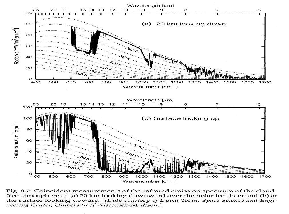
If you look at about 900 cm^-1, you see the atmospheric window. The air is transparent, and S-B from surface works. In the top plot, the radiation follows the S-B line for about 273K, the surface tempeerature. An looking up, it follows around 3K, space.
But if you look at 650 cm^-1, a peak CO2 frequency, you see that it is following the 225K line. That is the temperature of TOA. The big bite there represents the GHE. It’s that reduced emission that keeps us warm. And if you look up, you see it following the 268K line. That is the temperature of air near rhe ground, which is where that radiation is coming from. And so you see that, by eye, the intensity of radiation down is about twice up.
In this range radiation from the surface (high) is disconnected from what is emitted at TOA.

Reply to  Nick Stokes
January 5, 2017 8:41 pm

NIck,
You are conflating a Planck spectrum with conformance to SB. If you apply Wein’s displacement law the average radiation emitted by the planet, the color temperature of the planets emissions is approximately equal 287K while the EQUIVALENT temperature given by SB is about 255K owing to the attenuation you point out in the absorption bands. Moreover; as I said before, the attenuation in a absorption bands is only about 3db and it looks basically the same from 100km except for some additional ozone absorption.
Where do you think the 255K equivalent temperature representing the 240 W/m^2 emitted by the planet comes from?

Nick Stokes
Reply to  co2isnotevil
January 5, 2017 9:13 pm

George,
“Where do you think the 255K equivalent temperature representing the 240 W/m^2 emitted by the planet comes from?”
It’s an average. As you see from this clear sky spectrum, parts are actually emitted from TOA (225K) and parts from surface (273K). If you aggregate those as a total flux and put into S-B, you get T somewhere between. Actually, it’s more complicated because of clouds, which replace the surface component by something colder (top of cloud temp), and because there are some low OD frequencies where the outgoing emission comes from various levels.
But the key thing is that you can’t make your assumption that the atmosphere re-radiates equally up and down. It just isn’t so.

Reply to  Nick Stokes
January 5, 2017 9:27 pm

Nick,
“But the key thing is that you can’t make your assumption that the atmosphere re-radiates equally up and down. It just isn’t so.”
What do you think this ratio is if its not half up and half down?
The sum of what goes up and down is fixed and the more you think the atmosphere absorbs (Trenberth claims even more than 75%), the larger the fraction of absorption that must go up in order to acheive balance.

Nick Stokes
Reply to  co2isnotevil
January 5, 2017 9:38 pm

George,
“What do you think this ratio is if its not half up and half down?”
It’s frequency dependent. At 650 cm^-1, in that spectrum, it is 100:55. But it would be different elsewhere (than Barrow in spring), and at other frequencies. There is no easy way to deduce a ratio; you just have to add it all up. But 1:1 has no basis.

Reply to  Nick Stokes
January 5, 2017 9:53 pm

Nick,
“you just have to add it all up.”
Yes, and I’ve done this and its about 50/50, but it does vary spatially and temporally a little bit on either side and the as system varies this ratio, it almost seems like an internal control valve, none the less, it has a relatively unchanging long term average. But as I keep having to say, the climate sensitivity is all about changes to long term averages and long term averages are integrated over a whole number of years and over the relevant ranges of all the dependent variables they are dependent on.

Reply to  co2isnotevil
January 6, 2017 8:20 am

it almost seems like an internal control valve

That’s because there is one. https://micro6500blog.wordpress.com/2016/12/01/observational-evidence-for-a-nonlinear-night-time-cooling-mechanism/

Alex
Reply to  Nick Stokes
January 5, 2017 10:56 pm

The images are reading different things. Blind Freddy can see that they are the inverse of each other.
The only way you could get a spectrum like the 2nd image is by looking at the sun. Black space won’t give you that spectrum. Both images are looking through the atmosphere with a background ‘light’. Looking at the same thing -the atmosphere.
Please explain why the photons from the sun aren’t absorbed by the atmosphere while the photons from earth are.

Nick Stokes
Reply to  Alex
January 6, 2017 12:25 am

“Black space won’t give you that spectrum.”
You aren’t seeing black space, except in the atmospheric window (around 900 cm^-1). You are seeing thermally radiating gases, mainly CO2 and H2O. Unless you are Blind Freddy.

Alex
Reply to  Alex
January 6, 2017 12:34 am

Nick
Give me a link to the paper. I can’t find it. Don’t be rude. I actually like you, so don’t make enemies if you don’t have to. I feel that your ‘cut and paste’ from some source is biased (by someone). The 2 images you’ve shown are different. one is an emission spectrum and the other is an absorption spectrum. It’s clearly visible. I would like to reassure myself that the information is correct. I am certain that you would like some reassurance too

Alex
Reply to  Alex
January 6, 2017 12:49 am

Nick
You haven’t answered my question.
‘Please explain why the photons from the sun aren’t absorbed by the atmosphere while the photons from earth are.’

Nick Stokes
Reply to  Alex
January 6, 2017 1:37 am

Alex,
“Give me a link to the paper. “
It’s a textbook, here. And yes, one spectrum is looking down, the other up. It shows the GHG complementary emission from near surface air and TOA.
“Please explain why the photons from the sun aren’t absorbed by the atmosphere “
We’re talking about thermal IR. There just aren’t that many coming from the sun in that range, but yes, they are absorbed in that range.
Someone will probably say that at all levels emission increases with temperature, so the sun should be emitting more. Well, it emits more per solid angle. You get more thermal IR from the sun than from any equivalent patch of sky. But there is a lot more sky. Thermal IR from sun is a very small fraction of total solar energy flux.

Reply to  Nick Stokes
January 5, 2017 11:11 pm

Nick,
The other part of the question has not been addressed yet. While you don’t yet accept that the gray body model accurately reflects the relationship between the surface temperature and emissions of the planet and since in LTE Pin == Pout this relationship sets an upper bound on the sensitivity to forcing, how can you explain Figure 3 and especially the tight distribution of samples (red dots) around the predicted transfer characteristic (green line)? BTW, of all the plots I’ve done that show one climate variable against another, the relationship in Figure 3 has the tightest distribution of samples I’ve ever seen. It’s pretty undeniable.

Nick Stokes
Reply to  co2isnotevil
January 6, 2017 12:32 am

” While you don’t yet accept that the gray body model accurately reflects the relationship between the surface temperature and emissions of the planet”
Because the concepts are all wrong. You confound surface temperature with equivalent temperature. The atmosphere is nothing like what you model. It has high opacity in frequency bands, at which it is also highly radiative. It has a large range of vertical temperature variation. Surface temperatures are very largely set by the amount of IR that is actually emitted by lower levels of the atmosphere. And they of course depend on the surface.
At times you seem to say that you are just doing Trenberth type energy accounting. But Trenberth has no illusions that his accounting can determine sensitivity. The physics just isn’t there.

Reply to  Nick Stokes
January 6, 2017 12:40 am

“You confound surface temperature with equivalent temperature.”
The two track changes in each other exactly. It’s a simple matter to calibrate the absolute value.
“The atmosphere is nothing like what you model.”
I don’t model the atmosphere, I model the relative relationship between the boundaries of that atmosphere. One boundary at the surface and another at TOA. What happens between the surface and TOA are irrelevant, all the model cares about is what the end result is.
“It has high opacity in frequency bands, at which it is also highly radiative. It has a large range of vertical temperature variation.”
This is why averages are integrated across wavelength and other dependent variables. This way, the averages are wavelength independent as are all the other variables.
“Surface temperatures are very largely set by the amount of IR that is actually emitted by lower levels of the atmosphere.”,
No. Surface temperature are set by the amount of IR the surface radiates and absorbs, which in the steady state are equal. If it helps, consider a water world and/or worlds without water, GHG’s and/or atmospheres.

RW
Reply to  co2isnotevil
January 6, 2017 8:18 am

Nick,
Another way of looking at this:
The total IR flux emitted by the surface which is absorbed by the atmosphere is roughly 300 W/m^2, which happens to (coincidently) be roughly the same as the amount of IR the atmosphere as a whole mass passes to the surface.
You don’t really think or believe the contribution of 300 W/m^2 of DLR at the surface is entirely sourced from and driven by the re-radiation of this 300 W/m^2 initially absorbed by the atmosphere from the surface, do you? Clearly there would be contributions from all three energy flux input sources to the atmosphere — the energy of which also radiates downward toward and to the surface.
Keep in mind there are multiple energy inputs to the atmosphere besides just the upwelling IR emitted from the surface (and atmosphere) which is absorbed. Post albedo solar energy absorbed by the atmosphere and re-emitted downward to the surface would not be ‘back radiation’, but instead ‘forward radiation’ from the Sun whose energy has yet to reach the surface. And in addition to the radiant flux emitted from the surface which is absorbed there is significant non-radiant flux moved from the surface into the atmosphere, primarily as the latent heat of evaporated water, which condenses to forms clouds — whose deposited energy within (in addition to driving weather), also radiates substantial IR downward to the surface. The total amount of IR that is ultimately passed to the surface has contributions from all three input sources, and the contribution from each one cannot be distinguished or quantified in any clear or meaningful way from the other two.
Thus mechanistically, the downward IR flux ultimately passed to the surface from the atmosphere has no clear relationship to the underlying physics driving the GHE, i.e. the re-radiation of initially absorbed surface IR energy back downward where it’s re-absorbed at a lower point somewhere.
Thus it’s this re-radiated downward push of absorbed surface IR within the atmosphere that is slowing down the radiative cooling or resisting the huge upward IR push ultimately out the TOA. The total DLR at the surface is more just related to the rate the lower layers in combination with the surface are forced (from that downward re-radiated IR push) to be emitting up in order for the surface and the whole of the atmosphere to be pushing through the required 240 W/m^2 back into space.

RW
Reply to  Nick Stokes
January 6, 2017 7:59 am

Nick,
Yes, significantly more IR is passed to the surface from the atmosphere than is passed from the atmosphere into space, due to the lapse rate. Roughly a ratio of 2 to 1, or about 300 W/m^2 to the surface and 150 W/m^2 into space. However, if you add these together that’s a total of 450 W/m^2. The maximum amount of power that can be absorbed by the atmosphere (from the surface), i.e. attenuated from being transmitted into space, is about 385 W/m^2, which is also the net amount of flux that must exit the atmosphere at the bottom and be added to the surface in the steady-state. By George’s RT calculation, about 90 W/m^2 of the IR flux emitted by the surface is directly transmitted into space, leaving about 300 W/m^2 absorbed. This means that the difference of about 150 W/m^2, i.e. 450-300, must be part of a closed flux circulation loop between the surface and atmosphere, whose energy is neither adding or taking away joules from the surface or nor adding or taking away joules from the atmosphere.
Remember, not all of the 300 W/m^2 of IR passed to the surface from the atmosphere is actually added to the surface. Much of it is replacing non-radiant flux leaving the surface (primarily latent heat), but not entering the surface (as non-radiant flux). The bottom line is in the steady-state, any flux in excess of 385 W/m^2 leaving or flowing into the surface must be net zero across the surface/atmosphere boundary.
George’s ‘A/2’ or claimed 50/50 split of the absorbed 300 W/m^2 from the surface, where about half goes to space and half goes to the surface, is NOT a thermodynamically manifested value, but rather an abstract conceptual value based on a box equivalent model constrained by COE to produce a specific output at the surface and TOA boundaries.
Just because the atmosphere as a whole mass emits significantly more downward to the surface than upwards into space does NOT mean upwelling IR absorbed somewhere within has a greater chance of being re-radiated downwards than upwards. Whether a particular layer is emitting at 300 W/m^2 or 100 W/m^2, if 1 additional W/m^2 from the surface is absorbed, that layer will re-emit +0.5 W/m^2 up and +0.5 W/m^2 down. Meaning this is independent of the lapse rate. The re-emission of the absorbed energy from the surface, no matter where it goes or how long it persists in the atmosphere, is henceforth non-directional, i.e. occurs with by and large equal probability up or down. And it is this re-radiation of absorbed surface IR back downwards towards (and not necessarily back to) the surface that is the physical driver of the GHE or the underlying mechanism of the GHE that’s slowing down the radiative cooling of the system. NOT the total amount of IR the atmosphere as a whole mass passes to the surface.
The physical meaning of the ‘A/2’ claim or the 50/50 equivalent split is that not more than about half of what’s captured by GHGs (from the surface) is contributing to downward IR push in the atmosphere that ultimately leads to the surface warming, where as the other half is contributing to the massive cooling push the atmosphere makes by continuously emitting IR up at all levels. Or only about half of what’s initially absorbed is acting to ultimately warm the surface, where as the other half is acting to ultimately cool the system and surface.
I’ve noticed many people like yourself seem unable to separate radiative transfer in the atmosphere with the underlying physics of the GHE that ultimately leads to surface warming. The GHE is applied physics within the physics of atmospheric radiative transfer. Atmospheric radiative transfer is not itself (or by itself) the physics of the GHE. This means the underlying physics of the GHE are largely separate from the thermodynamic path manifesting the energy balance, and it is this difference that seems to elude so many people like yourself.

RW
Reply to  RW
January 6, 2017 9:07 am

Nick,
I assume it is agreed by you that the constituents of the atmosphere, i.e. GHGs and clouds, act to both cool the system by emitting IR up towards space and warm it by emitting IR downwards towards the surface. Right? George is just saying that like anything else in physics or engineering, this has to be accounted for, plain and simple.
He’s using/modeling the Earth/atmosphere system as a black box, constrained by COE to produce required outputs at the surface and TOA, given specific inputs:
https://en.wikipedia.org/wiki/Black_box
When this is applied to surface IR absorbed by the atmosphere, it yields that only about half of what’s absorbed by GHGs is acting to ultimately warm the surface, where as the other half is contributing to the radiative cooling push of the atmosphere and ultimate cooling of the system:
http://www.palisad.com/co2/div2/div2.html
George is not modeling the actual thermodynamics here and all the complexities associated with the thermodynamics (which isn’t possible by such methods), but rather he’s trying to isolate the effect the absorption of surface IR by GHGs, and the subsequent non-directional re-radiation of that absorbed energy, is having amongst the highly complex and non-linear thermodynamic path manifesting the surface energy balance, so far as its ultimate contribution to surface warming.

Reply to  Nick Stokes
January 6, 2017 9:47 am

Nick – that post and the info contained in those graphs are fantastically educational to me [just trying to learn here]. Now I must go and try to find the paper they came from. Just wanted to say that those observations and descriptions crystallize what is otherwise difficult to visualize [for a newbie]. Thanks much.

Reply to  Nick Stokes
January 6, 2017 11:49 am

Nick , are those spectra in a easily accessible tables somewhere ? Email me them or point me to them and I’ll calculate the actual radiative equilibrium temperature they imply .
co2isnotevil is right that “lapse rate” is the equilibrium expression of gravitational energy .
It cannot be explained as an optical phenomenon — which is why neither quantitative equation nor experimental demonstration of such a phenomenon has ever been presented .

Reply to  Bob Armstrong
January 6, 2017 12:29 pm

Bob,
A couple of things to notice about the spectra.
1) There is no energy returned to the surface in the transparent regions of the atmosphere. This means that no GHG energy is being ‘thermalized’ and re-radiated as broad band BB emissions.
2) The attenuation in absorption bands at TOA (20km is high enough to be considered TOA relative to the radiative balance) is only about 3db (50%). Again, if GHG energy was being ‘thermalized’, we would see littlle, if any, energy in the absorption bands, moreover; this is consistent with the 50/50 split of absorbed energy required by geometrical considerations.
3) The small wave number data (400-600) is missing from the 20km data looking down which would otherwise illustrates that the color temperature of the emissions (where the peak is relative to Wein’s Displacement Law) is the surface temperature and the 255K equivalent temperature is a consequence of energy being removed from parts of the spectrum manifesting a lower equivalent temperature for the outgoing radiation,
BTW, I’ve had discussions with Grant Perry about this and he has trouble moving away from this ‘thermalization’ point of view, despite the evidence. To be fair, it doesn’t really matter from a thermodynamic balance and temperature perspective (molecules in motion affect a temperature sensor in the same was a photons of the same energy), but only matters if you want to accurately predict the spectrum and account for 1), 2) and 3) above.
Of course, this goes against the CAGW narrative which presumes that GHG absorption heats the atmosphere (O2/N2) which then heats the surface by convection, rather then the purely radiative effect it is where photons emitted by GHG’s returning to the ground state are what heat the surface. One difference is that if all GHG absorption was ‘thermalized’ as the energy of molecules in motion, all must be returned to the surface, since molecules in motion do not emit photons that can participate in the radiative balance and there wouldn’t be anywhere near enough energy to offset the incoming solar energy.

Reply to  Bob Armstrong
January 6, 2017 12:29 pm

That is correct.
An atmosphere in hydrostatic equilibrium suspended off the surface by the upward pressure gradient force and thus balanced against the downward force of gravity will show a lapse rate slope related to the mass of the atmosphere and the strength of the gravitational field.
It is all a consequence of conduction and convection NOT radiation.
The radiation field is a mere consequence of the lapse rate slope caused by conduction and convection.
Radiation imbalances within an atmosphere simply lead to convection changes that neutralise such imbalances in order to maintain long term hydrostastic equilibrium.
No matter what the proportion of GHGs in an atmosphere the surface temperature does not change. Only the atmospheric convective circulation pattern will change.

Nick Stokes
Reply to  Bob Armstrong
January 6, 2017 2:44 pm

Bob A,
“Nick , are those spectra in a easily accessible tables somewhere ?”
Unfortunately not, AFAIK. As I mentioned above, the graph comes from a textbook. The caption gives an attribution, but I don’t think that helps. It isn’t recent.
I have my own notion of the lapse rate here, and earlier posts. Yes, the DALR is determined by gravity. But it takes energy to maintain it, and the flux that passes through with radiative transfer in GHG-active regions helps to maintain it.

Reply to  Nick Stokes
January 7, 2017 8:00 pm

This is one of the great atmospheric experiments of all time. I agree with everything you say except that 228K is the Arctic tropopause rather than the top of the atmosphere. The top of the atmosphere is more like 160K where water is radiating in the window.
The peak CO2 frequency is actually 667.4, close enough. You can see a little spike indicating the 667.4 Q branch. Looking up, it would ordinarily be pointed down. In this case a strong surface inversion reversed it.
Long wave infrared light only comes from the earth’s surface. It does not come from the sun. It is not manufactured by Carbon dioxide, or any other greenhouse gas. These gasses absorb and re-emit long wave radiation emitted from the surface according to their individual material properties.
You say it emits down more than it emits up. I say the two emissions are disconnected. The boundary layer extinguishes the 667.4 band. Radiation in the band resumes generally at about the cloud condensation level as a result of condensation energy. CO2 radiates from the tropopause because massive amounts of new energy are added by ozone absorption.

January 5, 2017 8:39 pm

Presence in the phrase “the Climate Sensitivity” of the word “the” implies existence of a fixed ratio between the change in in the spatially averaged surface air temperature at equilibrium and the change in the logarithm of the atmospheric CO2 concentration. Would anyone here care to defend the thesis that this ratio is fixed?

Reply to  Terry Oldberg
January 5, 2017 8:45 pm

Terry,
It’s definitely not a fixed ratio, either temporally or spatially, but it does have a relatively constant yearly average and changes to long term averages are all we care about when we are talking about the climate sensitivity. This is where superposition in the energy domain comes in which allows us to calculate meaningful averages since 1 Joule does 1 Joule of work and no more or no less.

Reply to  co2isnotevil
January 5, 2017 10:42 pm

Thank you, c02isnotevil, for taking the time to respond. That “1 Joule does 1 Joule of work” is not a principle of thermodynamics. Did you mean to say that “1 Joule of heat crossing the boundary of a concrete object does 1 Joule of work on this boundary absent change in the internal energy of this object”?

Reply to  Terry Oldberg
January 5, 2017 10:49 pm

The basic point is no 1 Joule is any different than any other.

Reply to  co2isnotevil
January 5, 2017 11:06 pm

That “no 1 Joule is any different than any other” is a falsehood.

Reply to  Terry Oldberg
January 5, 2017 11:26 pm

Terry,
Energy can not be created or destroyed, only transformed from one form to another. Different forms may be incapable of doing different kinds of work, but relative to the energy of photons, it’s all the same and photons are all that matter relative to the radiative balance and a quantification of the sensitivity. The point of this is that if each of the 240 W/m^2 of incident power only results in 1.6 W/m^2 of surface emissions, the next W/m^2 can’t result in more than 4 W/m^2 which is what the IPCC sensitivity requires. The average emissivity is far from being temperature sensitive enough.
If you examine the temp vs. emissivity plot I posted in response to one of Nick’s comments, the local minimum is about at the current average temperature and the emissivity increases (sensitivity decreases) whether the temperature increases or decreases, but not by very much.

phaedo
Reply to  Terry Oldberg
January 6, 2017 2:05 am

Terry Oldberg, ‘Presence in the phrase “the Climate Sensitivity” of the word “the” implies existence of a fixed ratio …’ Could you explain the reasoning that led you to that statement.

Reply to  phaedo
January 8, 2017 9:09 am

phaedo:
I can explain that. Thanks for asking.
Common usage suggests that “the climate sensitivity” references a fixed ratio, The change that is in the numerator of this ratio is the equilibrium temperature. Thus, this concept is often rendered as “ECS” but I prefer “TECS” (acronym for “the equilibrium climate sensitivity”) as this usage makes clear that a constant is meant.
Warmists argue that the value of TECS is about 3 Celsius per doubling of the CO2 concentration. Bayesians treat the ratio as a parameter having prior and posterior probability density functions indicating that they believe TECS to be a constant with uncertain value.
It is by treating TECS as a constant that climatologists bypass the thorny issue of variability. If TECS is only the ratio of two numbers then climatologists have to make their arguments in terms of probability theory and statistics but to avoid this involvement is a characteristic of their profession. For evidence, search the literature for a description of the statistical population of global warming climatology. I believe you will find, like me, that there isn’t one.

Reply to  Terry Oldberg
January 8, 2017 9:59 am

Warmists argue that the value of TECS is about 3 Celsius per doubling of the CO2 concentration. Bayesians treat the ratio as a parameter having prior and posterior probability density functions indicating that they believe TECS to be a constant with uncertain value.

I have an effective cs for to extratropics for the seasonal changes in calculated station solar and it’s actually change in temp here
http://wp.me/p5VgHU-1t

Reply to  micro6500
January 8, 2017 10:11 am

micro6500
That’s a good start on a statistical investigation. To take it to the next level I’d identify the statistical population, build a model from a sample drawn randomly from this population and cross validate this model in a different sample. If the model cross validates you’ve done something worth publishing. The model “cross validates” if and only if the predictions of the model match the observations in the second of the two samples. To create a model that cross validates poses challenges not faced by professional climatologists as their models are not falsifiable.

Reply to  Terry Oldberg
January 8, 2017 10:21 am

It does, it shows up as an exponential decay in cooling rates, and the some of the data (with net rad) was from Australia, and other temp charts are from data in Ohio. And it explains everything. (Clear sky cooling performance)

January 5, 2017 8:48 pm

The climate system has a couple positive feedbacks that do not violate any laws of physics. For one thing, the Bode feedback theory does not require an infinite power supply for positive feedback, not even for positive feedback with feedback factor exceeding 1. The power supply only has to be sufficient to keep the law of conservation of energy from being violated. There is even the tunnel diode oscillator, whose only components are an inductor and capacitor to form a resonator, two resistors where one of them nonlinear to have voltage and current varying inversely with each other over a certain range (the tunnel diode), and a power supply to supply the amount of current needed to get the tunnel diode into a mode where voltage across it and current passing through it vary inversely.
As for positive feedbacks in the climate system: One that is simple to explain is the surface albedo feedback. Snow and ice coverage vary inversely with temperature, so the amount of sunlight absorbed varies directly with temperature. This feedback was even greater during the surges and ebbings of Pleistocene ice age glaciations, when there was more sunlight-reflecting ice coverage that could be easily expanded or shrunk by a small change in global temperature. Ice core temperature records indicate climate that was more stable during interglacial periods and less stable between interglacials, and there is evidence that at some brief times during glaciations there were sudden climate shifts – when the climate system became unstable until a temporarily runaway change reduced a positive feedback that I think was the surface albedo one.
Another positive feedback is the water vapor feedback, which relates to the gray body atmosphere depiction in Figure 2. One thing to consider is that the gray body filter is a bulk one, and thankfully Figure 2 to a fair extent shows this. Another thing to consider is that this bulk gray body filter is not uniform in temperature – the side facing Earth’s surface is warmer than the side facing outer space, so it radiates more thermal radiation to the surface than to outer space. (This truth makes it easier to understand how the Kiehl Trenberth energy budget diagram does not require violation of any laws of physics for its numbers to add up with its attributions to various heat flows.)
If the world warms, then there is more water vapor – which is a greenhouse gas, and the one that our atmosphere has the most of and that contributes the most to the graybody filter Also, more water vapor means greater emissivity/absorption of the graybody filter depicted in Figure 2. That means thermal radiation photons emitted by the atmosphere reaching the surface are emitted from an altitude on-average closer to the surface, and thermal radiation photons emitted by the atmosphere and escaping to outer space are emitted from a higher altitude. So, more water vapor means the bulk graybody filter depicted in Figure 2 is effectively thicker, with its effective lower surface closer to the surface and warmer. Such a thicker denser effective graybody filter has increased inequality between its radiation reaching the surface and radiation escaping to outer space.

Reply to  Donald L. Klipstein
January 5, 2017 9:23 pm

Donald,
You are incorrect about Bode’s assumptions. They are laid out in the first 2 paragraphs in the book I referenced. Google it and you can find a free copy of it on-line. The requirement for a vacuum tube and associated power supply specifies the implicit infinite supply, as there are no restrictions on the output impedance in the Bode model, which can be 0 requiring an infinite power supply. This assumed power supply is the source of most of the extra 12+ W/m^2 required over and above the 3.7 W/m^2 of CO2 ‘forcing’ that is required in the steady state to sustain a 3C temperature increase. Only about 0.6W per W/m^2 (about 2.2 W/m^2) is all the ‘feedback’ the climate system can provide. Of course, the very concept of feedback is not at all applicable to a passive system like the Earth’s climate system (passive specifically means no implicit supply).
Regarding ice. The average ice coverage of the planet is about 13%, most of which is where little sunlight arrives anyway. It it all melted and considering that 2/3 of the planet is covered by clouds anyway and mitigates the effects of albedo ‘fedeback’, the incremental un-reflected input power can only account for about half of the 10 W/m^2 above and beyond the 2.2 W/m^2 from 3.7 W/m^2 of forcing based on 1.6 W/m^2 of surface emissions per W/m^2 of total forcing. This does become more important as more of the planet is covered by ice and snow, but at the current time, we are pretty close to minimum possible ice. No amount of CO2 will stop ice from forming during the polar winters.
Regarding water vapor. You can’t consider water vapor without considering the entire hydro cycle, which drives a heat engine we call weather which unambiguously cools based on the trails of cold water left in the wake of a Hurricane. The Second Law has something to say about this as well, where a heat engine can’t warm its source of heat.

Reply to  co2isnotevil
January 6, 2017 8:21 am

Amplifiers with positive feedback even to the point of instability or oscillation do not require zero output impedance, and they work in practice with finite power supplies. Consider the tunnel diode oscillator, where all power enters the circuit through a resistor. Nonpositive impedance in the tunnel diode oscillator is incremental impedance, and that alone being nonpositive is sufficient for the circuit to work.
Increasing the percentage of radiation from a bulk graybody filter of nonuniform temperature towards what warms its warmer side does not require violation of the second law of thermodynamics, because this does not involve a heat engine. The only forms of energy here are heat and thermal radiation – there is no conversion to/from other forms of energy such as mechanical energy. The second law of thermodynamics only requires net flow to be from warmer points and surfaces to cooler points and surfaces, which is the case with a bulk graybody filter with one side facing a source of thermal radiation that warms the graybody filter from one side. Increasing the optical density of that filter will cause the surface warming it to have a temperature increase in order to get rid of the heat it receives from a kind of radiation that the filter is transparent to, without any net flows of heat from anything to anything else that is warmer.
As for 2/3 of the Earth’s surface being covered by clouds: Not all of these clouds are opaque. Many of them are cirrus and cirrostratus, which are translucent. This explains why the Kiehl Trenberth energy budget diagram shows about 58% of incoming solar radiation reaching the surface. Year-round insolation reaching the surface around the north coast of Alaska and Yukon is about 100 W/m^2 according to a color-coded map in the Wikipedia article on solar irradiance, and the global average above the atmosphere is 342 W/m^2.

Reply to  Donald L. Klipstein
January 6, 2017 9:57 am

“Amplifiers with positive feedback even to the point of instability or oscillation do not require zero output impedance”
Correct, but Bode’s basic gain equation makes no assumptions about the output impedance and it can just as well be infinite or zero and it still works, therefore, the implicit power supply must be unlimited.
The Bode model is idealized and part of the idealization is assuming an infinite source of Joules powers the gain.
Tunnel diodes work at a different level based on transiently negative resistance, but this negative resistance only appears when the diode is biased, which is the external supply.
“Not all of these clouds are opaque.”
Yes, this is true and the average optical depth of clouds is accounted for by the analysis. The average emissivity of clouds given a threshold of 2/3 of the planet covered bu them, is about 0.7. Cloud emissivity approaches 1 as the clouds get taller and denser, but the average is only about 0.7. This also means that about 30% of surface emissions passes through clouds and this is something Trenberth doesn’t account for with his estimate of the transparent window.

Reply to  co2isnotevil
January 6, 2017 8:27 am

More on your statement that clouds cover 2/3 of the surface: You said “After accounting for reflection by the surface and clouds, the Earth receives about 240 W/m2 from the Sun”. That is 70% of the 342 W/m^2 global average above the atmosphere.

Reply to  co2isnotevil
January 6, 2017 11:04 am

co2isnotevil: Clouds can simultaneously have majority emissivity and majority transmission of incoming solar radiation. The conflict is resolved by incoming solar radiation and low temperature thermal radiation being at different wavelengths, and clouds have absorption/emissivity varying with wavelength while equal to each other, and higher in wavelengths longer than 1.5 micrometers (about twice the wavelength of border between visible and infrared) than in shorter wavelengths.

Reply to  Donald L. Klipstein
January 6, 2017 11:34 am

Donald,
“Clouds can simultaneously have majority emissivity and majority transmission of incoming solar radiation”
Yes, this is correct. But again, we are only talking about long term changes in averages and over the long term, the water in clouds is tightly coupled to the water in oceans and solar energy absorbed by clouds can be considered equivalent to energy absorbed by the ocean (surface), at least relative to the long term steady state and the short term hydro cycle.

Reply to  co2isnotevil
January 6, 2017 11:06 am

co2isnotevil: I did not state that a tunnel diode oscillator does not require a power supply, but merely that it does not require an infinite one. For that matter, there is no such thing as an infinite power supply.

Reply to  Donald L. Klipstein
January 6, 2017 11:40 am

Donald,
“there is no such thing as an infinite power supply.”
Correct, but we are dealing with idealized models based on simplifying assumptions, especially when it comes to Bode’s feedback system analysis. And one of the many simplifying assumptions Bode makes is that there is no limit to the Joules available to power the gain (unconstrained active gain). The error with how the climate was mapped to Bode was that the simplifying assumptions were not applicable to the climate system, thus the analysis is also not applicable.

Reply to  co2isnotevil
January 6, 2017 11:10 pm

co2isnotevil saying: “And one of the many simplifying assumptions Bode makes is that there is no limit to the Joules available to power the gain (unconstrained active gain). The error with how the climate was mapped to Bode was that the simplifying assumptions were not applicable to the climate system, thus the analysis is also not applicable.”
Please state how this is not applicable. Cases with active gain can be duplicated by cases with passive gain, for example with a tunnel diode. The classic tunnel diode oscillator receives all of its power through a resistor whose resistance is constant, so availability of energy/power is limited. The analogue to Earth’s climate system does not forbid positive feedback or even positive feedback to the extent of runaway, but merely requires such positive feedback to be restricted to some certain temperature range, outside of which the Earth’s climate is more stable.

prjindigo
January 5, 2017 8:58 pm

So where’s the density component of your equations? Density is regulated by gravity alone on Earth.

Reply to  prjindigo
January 5, 2017 9:12 pm

prjindigo,
The internals of the atmosphere, which is where density comes in, are decoupled from the model which is a model that matches the measured transfer function of the atmosphere which quantifies the causal behavior between the surface temperature and output emissions of the planet. This basically sets the upper limit on what the sensitivity can be. The lower limit is the relationship between the surface temperature and the post albedo input power, whose slope is 0.19 C per W/m^2 which is actually the sensitivity of an ideal BB at the surface temperature! This is represented by the magenta line in Figure 3. I didn’t bring it up because getting acceptance for 0.3C per W/m^2 is a big enough hill to climb.

January 5, 2017 9:05 pm

Forrest,
The satellite data itself doesn’t say much explicitly, but it does report GHG concentrations (H2O and O3) and when I apply a radiative transfer model driven by HITRAN absorption line data (including CO2 and CH4) to a standard atmosphere with measured clouds, I get about 74%, which is well within the margin of error.

January 5, 2017 9:13 pm

A black body is nearly an exact model for the Moon.
By looking out my window I can see that this is not the case, it’s clearly a gray body.
A perfect blackbody is one that absorbs all incoming light and does not reflect any.

Reply to  Phil.
January 5, 2017 9:32 pm

Phil,
“By looking out my window I can see that this is not the case, it’s clearly a gray body.”
Technically yes, if we count reflection as not being absorbed per the wikipedia definition, it would be a gray body, but relative to the energy the Moon receives after reflection, it is a nearly perfect black body, so the calculations reduce the solar energy to compensate. BTW, I don’t really like the wikipedia definition which seems to obfuscate the applicability of a gray body emitter (black body source with a gray body atmosphere).

Reply to  co2isnotevil
January 5, 2017 10:34 pm

This is the trouble that comes when not properly allowing for the frequency dependence of ε. For the Moon, in the SW we see absorption and reflection (but not emission), which is fairly independent of frequency in that range. But ε changes radically getting into thermal IR frequencies, where we see pretty much black body emission.

Reply to  Nick Stokes
January 5, 2017 10:40 pm

“allowing for the frequency dependence of ε.”
The average ε is frequency independent and that is all the model depends on.
Why is it so hard to grasp that this model is concerned only with long term averages and that yes, every parameter is dependent on almost every other parameter, but they all have relatively constant long term averages. This is why we need to do the analysis in the domain of Joules where superposition applies since if 1 Joule can to X amount of work, 2 Joules can to 2X amount of work and it takes work to warm the surface and keep it warm and the sensitivity is all about doing incremental work. So many of you can’t get your heads out of the temperature domain which is highly non linear where superposition does not apply.

Reply to  co2isnotevil
January 9, 2017 6:34 am

co2isnotevil January 5, 2017 at 9:32 pm
Phil,
“By looking out my window I can see that this is not the case, it’s clearly a gray body.”
Technically yes, if we count reflection as not being absorbed per the wikipedia definition, it would be a gray body, but relative to the energy the Moon receives after reflection, it is a nearly perfect black body, so the calculations reduce the solar energy to compensate.

If you’re going to do a scientific post then get the terminology right, the moon is not a black body it’s a grey body. The removal of the reflected light is exactly what a greybody does, the blackbody radiation is reduced by the appropriate fraction in the gray body, that’s what the non unity constant is for. Also the atmosphere is not a greybody because its absorption is frequency dependent.

Reply to  Phil.
January 9, 2017 10:39 am

Phill,
“The removal of the reflected light is exactly what a greybody does”
This is not the only thing that characterizes a gray body. Energy passed through a semi-transparent body also implements grayness as does energy received by a body that does work other than affecting the bodies temperature (for example, photosynthesis).
My point is that if you don’t consider reflected input, the result is indistinguishable from a BB. And BTW, there is no such thing as an ideal BB in nature. All bodies are gray. Considering something to be EQUIVALENT a body black is a simplifying abstraction and this is what modelling is all about.
I don’t understand why the concept of EQUIVALENCE is so difficult for others to understand as without understanding EQUIVALENCE there’s no possibility of understanding modelling.

Reply to  co2isnotevil
January 9, 2017 12:02 pm

I don’t understand why the concept of EQUIVALENCE is so difficult for others to understand as without understanding EQUIVALENCE there’s no possibility of understanding modelling.

Just to be clear for me, I understand equivalency very well. I also understand fidelity, and reusability.
I’m just trying to understand and discuss the edges that define that fidelity.

Nick Stokes
January 5, 2017 9:24 pm

“A gray body emitter is one where the power emitted is less than would be expected for a black body at the same temperature.”
A gray body emitter has a rather specific meaning, not observed here. The power is less, but uniformly distributed over the spectrum. IOW, ε is independent of frequency. This is very much not true for radiative gases.
“Trenberth’s energy balance lumps the return of non radiant energy as part of the ‘back radiation’ term, which is technically incorrect since energy transported by matter is not radiation.”
A flux is a flux. Trenberth is doing energy budgetting; he’s not restricting to radiant. The discussion here is wrong. Material transport does count; it helps bring heat toward TOA, so to maintain the temperature at TOA as it loses heat by radiation.

Nick Stokes
Reply to  Nick Stokes
January 5, 2017 9:32 pm

Wiki’s article on black body is more careful and correct. It says “A source with lower emissivity independent of frequency often is referred to as a gray body.”. The independence is important.

Reply to  Nick Stokes
January 7, 2017 8:41 pm

“It is why 11 μ with ε = 0, IR goes straight from surface to space, while at 15μ, where ε is high, IR is radiated from TOA and not lower, because the atmosphere is opaque.”
The energy of ALL light is frequency dependent regardless the color (black or grey) of the emitting body. Emissivity has nothing to do with frequency, except as regards the wavelengths the emitting body happens to absorb and emit.
Wiki simply has it wrong.
CO2 has very LOW emissivity at about 15 microns. Otherwise it would not be extinguished within a meter of standard atmosphere. In order for surface energy to travel to the tropopause at 15 microns it would have to TRANSMIT. It doesn’t. Transmission is 1-absorption. There is ZERO transmission to the tropopause at 15/667.4. From Science of Doom:comment image

Reply to  Nick Stokes
January 9, 2017 12:12 pm

gymnosperm
Where did this graph come from?comment image
I would expect to find that the std atm had conditions that would lead to near 100% rel humidity for this spectrum. Do you have a link to the data to see exactly what they were doing with it.
This is what I’ve been blathering about, Or I don’t understand just exactly what (or where?) is being measured here. If this is surface up to space, it should only be like this if the rel humidity is pretty high.

Reply to  micro6500
January 9, 2017 12:42 pm

micro6500,
This plot looks like the inverse of absorption, which is not specifically transmission since transmission includes the fraction of absorption that is eventually transmitted into space.

Reply to  co2isnotevil
January 9, 2017 2:41 pm

Except it isn’t just co2.comment image

Reply to  Nick Stokes
January 5, 2017 9:44 pm

“The power is less, but uniformly distributed over the spectrum”
As I pointed out, this is not a requirement. Joules are Joules and the frequency of the photons transporting those Joules is irrelevant relative to the energy balance and subsequent sensitivity. Again, the 240 W/m^2 of emissions we use SB to convert to an EQUIVALENT temperature of 255K is not a Planck distribution, moreover; the average emissivity is spectrally independent since it’s integrated across the entire spectrum.
“Material transport does count”
Relative to the radiant balance of the planet and the consequential sensitivity, it certainly does, since only photons can enter or leave the top boundary of the atmosphere. Adding a zero sum source and sink of energy transporter by matter to the radiant component of the surface flux shouldn’t make a difference, but it adds a layer of unnecessary obfuscation that does nothing but confuse people. The real issue is that he calls the non radiant return of energy to the surface radiation which is misrepresentative at best.

Reply to  co2isnotevil
January 5, 2017 10:39 pm

“As I pointed out, this is not a requirement.”
It is a requirement of the proper definition of grey body. It is why grey, as opposed to blue or red. And it is vitally important to atmospheric radiative transport. It is why 11 μ with ε = 0, IR goes straight from surface to space, while at 15μ, where ε is high, IR is radiated from TOA and not lower, because the atmosphere is opaque.

Reply to  Nick Stokes
January 5, 2017 10:48 pm

Nick,
“It is a requirement of the proper definition of grey body.”
Then the association between 255K and the average 240 W/m^2 emitted by the planet is meaningless as is the 390 W/m^2 (per Trenberth) emitted by the surface (he uses about 287.5K).
There is no requirement for a Planck distribution when calculating the EQUIVALENT temperature of matter based on its radiative emissions. This is what the word EQUIVALENT means. That is, an ideal BB at the EQUIVALENT temperature (or a gray body at an EQUIVALENT temperature and EQUIVALENT emissivity) will emit the same energy flux as the measured radiative emissions, albeit with a different spectra.

Reply to  co2isnotevil
January 5, 2017 11:45 pm

“Then the association between 255K and the average 240 W/m^2 emitted by the planet is meaningless…”
Nobody thinks that there is actually a location at 255K which emits the 240 W/m2.
“as is the 390 W/m^2 (per Trenberth) emitted by the surface (he uses about 287.5K).”
No, the surface is a black body (very dark grey) in thermal IR. It is a more or less correct application of S-B, though the linearising of T^4 in averaging involves some error.
“Planck distribution when calculating the EQUIVALENT temperature of matter”
You can always calculate an equivalent temperature. It’s just a rescaled expression of flux, as shown on the spectra I included. But there is no point in defining sensitivity as d flux/d (equivalent temperature). That is curcular. You need to identify the ET with some real temperature.

Reply to  Nick Stokes
January 6, 2017 12:07 am

“But there is no point in defining sensitivity as d flux/d (equivalent temperature)”
But, this is exactly what the IPCC defines as the sensitivity because dFlux is forcing. The idea of representing the surface temperature as an equivalent temperature of an ideal BB is common throughout climate science on both sides of the debate. It works because the emissivity of the surface itself (top of ocean + bits of land that poke through) is very close to 1. Only when an atmosphere is layered above it does the emissivity get reduced.

Nick Stokes
Reply to  co2isnotevil
January 6, 2017 12:21 am

” this is exactly what the IPCC defines as the sensitivity “
Not so. I had the ratio upside down, it is dT/dP. But T is measured surface air temperature, not equivalent temperature. We know how equivalent temp varies with P; we have a formula for it. No need to measure anything.

Reply to  Nick Stokes
January 6, 2017 12:30 am

“But T is measured surface air temperature, not equivalent temperature. ”
T is the equivalent surface temperature which is approximately the same as the actual near surface temperature measured by thermometers. This is common practice when reconstructing temperature from satellite data and the fact that they are close is why it works.

Tony
January 5, 2017 9:43 pm

“… doubling CO2 is equivalent to 3.7 W/m2 of incremental, post albedo solar power”
The sun when moving from its perihelion to aphelion each year produces as change of a massive 91 W/m2. It has absolutely ZERO impact on global temperatures, thanks to the Earth’s negative feedbacks.
Why does everyone keep ignoring them?

Reply to  Tony
January 5, 2017 10:20 pm

“It has absolutely ZERO impact on global temperatures”
The difference gets buried in seasonal variability since perihelion is within a week and a half of the N hemisphere winter solstice and the difference contributes to offset some of the asymmetry between the response of the 2 hemispheres. In about 10K years, it will be reversed and N hemisphere winters will get colder as its summers get warmer, while the reverse happens in the S hemisphere.

Jocelyn
Reply to  Tony
January 5, 2017 10:28 pm

Tony,
The closest (most heat rays from the sun) is in Jan. So you could think the global temperature would be the warmest then. But it is in July.
See here;
http://data.giss.nasa.gov/gistemp/news/20160816/july2016.jpg
I think the difference is mainly due to the difference in the amount of continent surface in the Northern Hemisphere vs the South.

hanelyp
January 5, 2017 10:18 pm

Where does convection as a heat transfer mechanism enter the model?

Reply to  hanelyp
January 5, 2017 10:25 pm

hanelyp,
Convection and heat transfer are internal to the atmosphere and the model only represents the results of what happens in the atmosphere, not how it happens. Convection itself is a zero sum influence on the radiant emissions from the surface since what goes up must come down (convection being energy transported by matter) and whatever effect it has is already accounted for by the surface temperature and its consequent emissions.

Reply to  co2isnotevil
January 5, 2017 11:36 pm

“since what goes up must come down (convection being energy transported by matter) “
That’s just not true. Trenberth’s fluxes are in any case net (of up and down). Heat is transported up (mainly by LH); the warmer air at altitude then emits this heat as IR. It doesn’t go back down.

Reply to  Nick Stokes
January 5, 2017 11:57 pm

Nick,
“Heat is transported up”
The heat you are talking about is the kinetic energy consequential to the translational motion of molecules which has nothing to do with the radiative balance or the sensitivity. Photons travel in any direction at the speed of light and I presume you understand that O2 and N2 neither absorb or emit photons in the relevant bands.

Nick Stokes
Reply to  co2isnotevil
January 6, 2017 12:10 am

” the kinetic energy consequential to the translational motion of molecules which has nothing to do with the radiative balance or the sensitivity”
It certainly does. I don’t think your argument gets to sensitivity at all. But local temperature of gas is translated directly into IR emission. It happens through GHgs; they are at the same temperature as O2 and N2. They emit according to that temperature, and the heat they lose is restored to them by collision with N2/O2, so they can emit again.

Reply to  Nick Stokes
January 6, 2017 12:28 am

Nick,
“But local temperature of gas is translated directly into IR emission. It happens through GHgs; they are at the same temperature as O2 and N2. They emit according to that temperature, and the heat they lose is restored to them by collision with N2/O2, so they can emit again.”
The primary way that an energized GHG molecule reverts to the ground state upon collision with O2 or N2 is by emitting a photon and only a fraction of the collisions have enough energy to do this. You do understand that GHG absorption/emission is a quantum state change that is EM in nature and all of the energy associated with that state change must be absorbed or emitted at once. There is no mechanism which converts any appreciable amount of energy associated with such a state change into linear kinetic energy at the relevant energies. At best, only small amounts at a time can be converted and its equally probably to increase the velocity as it is to decrease it. This is the mechanism of collisional broadening which extends the spectrum mostly symmetrically around resonance and which either steals energy or gives up energy upon collision, resulting in the emission of a slightly different frequency photon.

angech
January 5, 2017 10:28 pm

“A black body is nearly an exact model for the Moon.”
No, The moon is definitely not a black body.
Geometric albedo Moon 0.12 earth 0.434
Black-body temperature (K) Moon 270.4 earth 254.0

“To conceptualize a gray body radiator, If T is the temperature of the black body, it’s also the temperature of the input to the gray body,To be consistent with the Wikipedia definition, the path of the energy not being absorbed is omitted.”
This misses out on the energy defected back to the black body which is absorbed and remitted some of which goes back to the grey body. I feel this omission should at least be noted [I see reference to back radiation later in the article despite this definition]

” while each degree of warmth requires the same incremental amount of stored energy, it requires an exponentially increasing incoming energy flux to keep from cooling.”
It requires an exponentially increasing energy flux to increase the amount of stored energy, the energy flux must merely stay the same to keep from cooling.

“The equilibrium climate sensitivity factor (hereafter called the sensitivity) is defined by the IPCC as the long term incremental increase in T given a 1 W/m2 increase in input, where incremental input is called forcing”.
but, I am lost. The terms must sound similar but mean different things.
The equilibrium climate sensitivity (ECS) refers to the equilibrium change in global mean near-surface air temperature that would result from a sustained doubling of the atmospheric (equivalent) carbon dioxide concentration (ΔTx2). a forcing of 3.7 W/m2

“The only place for the thermal energy to go, if not emitted, is back to the source ”
Well it could go into a battery, but if not emitted it could never go back to the source.

“A gray body emitter is one where the power emitted is less than would be expected for a black body at the same temperature”.
At the same temperature both a grey and a black body would emit the same amount of power.
The grey body would not get to the same temperature as the black body from a constant heat source because it is grey, It has reflected, not absorbed, some of the energy. The amount of energy detected would be the same but the spectral composition would be quite different with the black body putting out far more infrared.

January 5, 2017 10:37 pm

“Both warm the surface by absorbing some fraction of surface emissions and after some delay, recycling about half of the energy back to the surface.”
Unfortunately, when energy is emitted by the surface, the temperature must fall. Half the emitted energy returning will not return the temperature to its pre emission state.
No increase in temperature. Night is an example. Or, temperatures falling after daytime maxima.
Cheers,

Phillip Bratby
January 5, 2017 10:50 pm

Anything based on the Earth’s average temperature is simply wrong.

Reply to  Phillip Bratby
January 5, 2017 10:56 pm

“Anything based on the Earth’s average temperature is simply wrong.”
This is why a proper analysis must be done in the energy domain where superposition applies because average emissions do represent a meaningful average. Temperature is just a linear mapping of stored energy and a non linear mapping to emissions which is why average temperature is not necessarily meaningful. It’s best to keep everything in the energy domain and convert average emissions to an EQUIVALENT average temperature in the end.

angech
January 5, 2017 11:24 pm

“Clouds also manifest a conditional cooling effect by increasing reflection unless the surface is covered in ice and snow when increasing clouds have only a warming influence.”
Clouds reflect energy regardless of ice and snow cover on the ground,They always have an albedo cooling effect. Similarly clouds always have a warming effect on the ground whether the surface is ice and snow or sand or water. The warming effect is due to back radiation from absorbed infrared , not the surface conditions. The question is what effect does it have on emitted radiation.

“Near the equator, the emissivity increases with temperature in one hemisphere with an offsetting decrease in the other. The origin of this is uncertain”
More land in the Norther Hemisphere means the albedo of the two hemispheres is different, The one with the higher albedo receives less energy to absorb and so emits less.

Reply to  angech
January 5, 2017 11:48 pm

angech,
“Clouds reflect energy regardless of ice and snow cover on the ground,”
Yes, but what matters is the difference in reflection between whether the cloud is present or not. When the surface is covered by ice and snow and after a fresh snowfall, cloud cover often decrease the reflectivity!
Yes, the land/sea asymmetry between hemispheres is important, especially at the poles and mid latitudes which are almost mirror images of each other, but where this anomaly is, the topological differences between hemispheres are relatively small.

angech
Reply to  co2isnotevil
January 6, 2017 1:26 am

co2isnotevil “Clouds reflect energy regardless of ice and snow cover on the ground,”
“Yes, but what matters is the difference in reflection between whether the cloud is present or not. When the surface is covered by ice and snow and after a fresh snowfall, cloud cover often decreases the reflectivity!”
Hm.
The clouds have already reflected all the incoming energy that they can reflect.Hence the ice and snow are receiving less energy than they would have.
Some of the radiation that makes it through and reflects will then reflect back to the ground and hence warm the surface again. Yes.Most will go out but I get your drift.
The point though is that it can never make the ground warmer than it would be if there was no cloud present. Proof ad absurdio would be if the cloud was totally reflective, no light, ground very cold, a slight bit of light a bit warmer, no cloud warmest.

Reply to  angech
January 6, 2017 9:02 am

“The point though is that it can never make the ground warmer than it would be if there was no cloud present.”
Not necessarily. GHG’s work just like clouds with one exception. The water droplets in clouds are broad band absorbers and broadband Planck emitters while GHG’s are narrow band line absorbers and emitters.

Tom in Oregon City
January 5, 2017 11:27 pm

“If T is the temperature of the black body, it’s also the temperature of the input to the gray body, thus Equation 1 still applies per Wikipedia’s over-constrained definition of a gray body.”
That’s just wrong.
Radiant energy has no temperature, only energy relative to its wavelength (to have temperature, there must be a mass involved). The temperature of the absorbing surface of that energy is dependent on its emissivity, its thermal conductivity, and it’s mass.

Reply to  Tom in Oregon City
January 5, 2017 11:52 pm

Tom,
“Radiant energy has no temperature, …”
Radiant energy is a remote measurement representative of the temperature of matter at a distance.

Tom in Oregon City
Reply to  co2isnotevil
January 6, 2017 5:04 pm

There’s no need to quote the texbook understanding of blackbody radiation spectrum to me. Observing the peak wavelength may tell you the temperature of a blackbody, but not the temperature it will generate at the absorber. Consider this: an emitter at temperature T, with a surface area A, emits all its energy toward an absorber with surface area 4A. What is the temperature of the absorber? Never T. It’s not the WAVELENGTH of the photons that determines the temperature of the absorber, it’s the flux density of photons, or better the total energy those photons — of any wavelength — present to the absorber, that determines the heat input to that absorber. Distance from the emitter, the emissivity of the absorber, its thermal conductivity, its total mass… all these things affect the TEMPERATURE of that grey body.
Consider it another way: take an object with Mass M and perfect thermal conductivity at temperature T, and allow it to radiate only toward another object of the same composition with mass 10M at initial temperature 0K. Will the absorber ever get hotter then T/10?
I repeat: those photons do not have temperature. Only matter has temperature.
Or would you care to tell me the temperature of microwave emissions from the sun? Certainly not 5778K.

angech
January 5, 2017 11:44 pm

“Trenberth’s energy balance lumps the return of non radiant energy as part of the ‘back radiation’ term, which is technically incorrect since energy transported by matter is not radiation.”
Trenberth shows the non radiant energy going out to space as radiation [ not “back radiating”]
Trenberth is simply getting the non radiant energy higher in the atmosphere where it eventually becomes radiative energy out to space [of course it does some back radiating itself as radiant energy but this part is included in his general back radiation schemata] . He is technically correct.

Reply to  angech
January 6, 2017 12:03 am

angech,
“He is technically correct.”
Latent heat cools the surface water as it evaporates and warms the droplet of water it condenses upon which returns to the surface as rain at a temperature warmer than it would be without the latent heat. The difference in what it would have been had all the latent heat been returned drives weather and is returned as gravitational potential energy (hydro electric power). The energy returned by the liquid water rain is not radiative, but nearly all the energy of that latent heat is returned to the surface as weather, including rain and the potential energy of liquid water lifted against gravity.

Tom in Oregon City
Reply to  co2isnotevil
January 6, 2017 5:09 pm

“Latent heat cools the surface water as it evaporates and warms the droplet of water it condenses upon which returns to the surface as rain at a temperature warmer than it would be without the latent heat.”
Where do you find such a description? Latent heat is released in order for water vapor to condense into liquid water again, and that heat is radiated away. Have you not noticed that water vapor condenses on cold surfaces, thus warming them? At the point of condensation the latent heat is lost from the now-liquid water, not when it strikes the earth again as rain.

Reply to  Tom in Oregon City
January 6, 2017 5:35 pm

Tom,
“… that heat is radiated away. ”
Where do you get this? How was water vapor radiate away latent heat? When vapor condenses, that heat is returns to the water is condenses upon and warms it. Little net energy is actually ‘radiated’ away from the condensing water since that atmospheric water is also absorbing new energy as it radiates stored energy consequential to its temperature. In LTE, absorption == emission and LTE sensitivity is all we care about.

Tom in Oregon City
Reply to  co2isnotevil
January 6, 2017 8:22 pm

This is quite pointless. Pick up a physics book, and figure out how the surface of water is cooled by evaporation: it is because in order for a molecule of water to leave the surface and become water vapor, it must have sufficient energy to break its bonds to the surface. This is what we call the heat of evaporation, or latent heat: water vapor contains more energy than liquid water at the same temperature. When water vapor condenses back into water, the energy that allowed it to become vapor is radiated away. It does not stay because… then the molecule would still be vapor.
Your avatar, co2isnotevil, I completely agree with. Where you got your information about thermal energy in the water cycle, or about the “temperature” of radiative energy, that I cannot guess. Not out of a Physics book. But I have seen similar errors among those who do not believe that radiative energy transactions in the atmosphere have any effect on the surface temperature at all, even when presented with evidence of that radiative flux striking the surface from the atmosphere above. And in that crowd, understanding of thermodynamics is sorely lacking.

Reply to  Tom in Oregon City
January 7, 2017 9:28 am

Tom,
You didn’t answer my question. You assert that latent heat is somehow released into the atmosphere BEFORE the phase change. No physics text book will make this claim. I suggest that you perform this
experiment:

Now, why is the phase change from vapor to liquid any different, relative to where the heat ends up?

Tom in Oregon City
Reply to  co2isnotevil
January 8, 2017 9:59 pm

co2isnotevil wrote “You assert that latent heat is somehow released into the atmosphere BEFORE the phase change.”
That is incorrect. The phase change forces the release of the latent heat, which itself was captured at the point of escape from the liquid state. But of course, that’s not the only energy change a molecule of water vapor undergoes on its way from the surface liquid state it left behind to the liquid state it returned to at sufficient altitude: there are myriad collisions along the way, each capable of either raising or lowering the energy of that molecule, along with radiative energy transactions where the molecule can either gain or lose energy. But we are talking about the AVERAGE here, for that is what TEMPERATURE is: an average energy measurement of some number of molecules, none of which must be at that exact temperature state.
Your experiment shows nothing outrageous or unexpected: the latent heat of fusion (freezing) is 334 joules, or 79.7 calories, per gram of water, while it takes only 1 calorie to raise the temperature of one gram of water by 1 degree. Therefore, as the water freezes to ice, those ice molecules are shedding latent heat even without changing temperature, and the remaining water molecules — and the temperature probe as well as the container — were receiving that heat. Thermal conductivity slows the probe’s reaction to changes in environment, and your experiment no longer shows something unexpected. Only your interpretation is unexpected, frankly.
The heat of fusion is much smaller than the heat of vaporization, which is 2,230 joules, or 533 calories, per gram.
Latent heat is not magic, or even complicated. Water becoming water vapor chills the surface, the vapor carries the heat aloft, where it is released by the action of condensation. Any Physics text — or even “Science” books from elementary school curricula — will bear out this definition.

Reply to  Tom in Oregon City
January 8, 2017 10:27 pm

“Water becoming water vapor chills the surface, the vapor carries the heat aloft, where it is released by the action of condensation.”
I would say this,
Evaporation cools by taking energy from the shared electron cloud of the liquid water that’s evaporating, the vapor carries the latent heat aloft, where the action of condensation adds it to the energy of the shared electron cloud of the water droplet it condenses upon, warming it.
The water droplet collides with other similarly warmed water droplets (no net transfer here) and with colder gas molecules (small transfer here). Of course, any energy transferred to a gas molecule is unavailable for contributing to the radiative balance unless it’s returned back to some water capable of radiating it away.

Tom in Oregon City
Reply to  co2isnotevil
January 8, 2017 10:43 pm

The only part you got right: “the vapor carries the latent heat aloft”
“shared electron cloud” — you write as if you believe liquid water is one gigantic molecule.
You neglect the physics of collisions, and the pressure gradients of the atmosphere, and pretend latent heat all returns to earth in rain. Liquid water emits radiation, “co2isnotevil”. Surely you know this. That radiative emission spreads in all directions, with a large part of it escaping from space.
I’m done. I’ve already said this discussion is pointless, and I’ve wasted more than enough time. My physics books don’t read like you do; I’ll stick with them.

Reply to  Tom in Oregon City
January 8, 2017 10:57 pm

“you write as if you believe liquid water is one gigantic molecule.”
You’re being silly. But you do understand that the difference between a liquid and a gas is that the electrons clouds of individual molecules strongly interact, while in a gas, the only such interactions are elastic collisions where they never get within several molecular diameters of each other. This is also true for a solid, except that the molecules themselves are not free to move.
Think about how close together the molecules in water are. So much so that when it freezes into a solid, it expands.

john harmsworth
Reply to  co2isnotevil
January 6, 2017 7:12 pm

Water vapour will condense under conditions of atmosphere cooler than it’s gaseous state. It most certainly not warm as a function of condensing. It will give up latent heat to sensible heat in the surrounding medium. This is generally at altitude where much of this heat will radiate away to space.

Reply to  john harmsworth
January 6, 2017 8:07 pm

John,
“It will give up latent heat to sensible heat in the surrounding medium.”
The ‘medium’ is the water droplet that the vapor condenses on.
When water evaporates, it cools the water it evaporated from. When water freezes, the ice warms, just as when water condenses, the water it condenses upon warms. When ice melts, the surrounding ice cools. This is how salting a ski run works in the spring to solidify the snow.
The latent heat is not released until the phase change occurs, which is why it’s called ‘latent’.
What physical mechanism do you propose allows the latent heat to instantly heat the air around it when water vapor condenses?

Nick Stokes
Reply to  co2isnotevil
January 7, 2017 11:27 am

“What physical mechanism do you propose allows the latent heat to instantly heat the air around it when water vapor condenses?”
The latent heat goes into the environment, bubble and air. On this scale, diffusion is fast. There is no unique destination for it. Your notion that the drops somehow retain the heat and return it to the surface just won’t work. The rain is not hot. Drops quickly equilibrate to the temperature of the surrounding air. On a small scale, radiation is insignificant for heat transfer compared to conduction.
Condensation often occurs in the context of updraft. Air is cooling adiabatically (pressure drop), and the LH just goes into slowing the cooling.

Reply to  Nick Stokes
January 7, 2017 12:00 pm

“Your notion that the drops somehow retain the heat and return it to the surface just won’t work.”
Did you watch or do the experiment?
You’re claiming diffusion, but that requires collisions between water droplets and since you do not believe the heat is retained by the water, how can diffusion work?
The latent heat per H2O molecule is about 1.5E-19 joules. The energy of a 10u photons (middle of LWIR range of emissions) is about 2E-20 joules. Are you trying to say that upon condensation, at many LWIR photons are instantly released? Alternatively, the kinetic energy of an N2 or O2 molecule in motion at 343 m/sec is about 2.7E-20 joules, so are you trying to say that the velocity of the closest air molecule more than doubles? What laws of physics do you suggest explains this?
How does this energy leave the condensed water so quickly? And BTW, the latent heat of evaporation doesn’t even show up until the vapor condenses on a water droplet, so whatever its disposition, it starts in the condensing water.

angech
January 5, 2017 11:52 pm

“The complex General Circulation Models used to predict weather are the foundation for models used to predict climate change. They do have physics within them, but also have many buried assumptions, knobs and dials that can be used to curve fit the model to arbitrary behavior. The knobs and dials are tweaked to match some short term trend, assuming it’s the result of CO2 emissions, and then extrapolated based on continuing a linear trend. The problem is that there as so many degrees of freedom in the model, it can be tuned to fit anything while remaining horribly deficient at both hind casting and forecasting.”
Spot on.
I think the stuff about the simple grey body model contains some good ideas on energy balance but needs to be put together in a better way without the blanket statements.
“The Earth can be accurately modeled as a black body surface with a gray body atmosphere, whose combination is a gray body emitter whose temperature is that of the surface and whose emissions are that of the planet. ”
Accurate modelling is not possible with such a complex structure though well described.

Reply to  angech
January 6, 2017 12:13 am

“Accurate modelling is not possible with such a complex structure though well described.”
Unless it matches the data which Figure 3 tests and undeniably confirms the prediction of this model. As I also pointed out, I’ve been able to model the temperature dependence of the emissivity and the model matches the data even better. How else can you explain Figure 3?
Models are only approximations anyway and the point is that this approximation, as simple as it is, has remarkable predictive power, including predicting what the sensitivity must be.

Reply to  angech
January 6, 2017 9:35 am

The GCMs do not actually forecast. They equivocate, which is not the same concept.

john harmsworth
Reply to  Terry Oldberg
January 6, 2017 7:14 pm

Hah! It’s forecasting without all that silly accountability!

Reply to  john harmsworth
January 6, 2017 10:01 pm

Right!

Brett Keane
January 6, 2017 12:27 am

When we remember that radiant energy is only a result of heat/temperature/ kinetic vibration rates in EM Fields, not a cause; we can start to avoid the tail-chasing waste of time that is modern climate ‘science’. When? Soon please.

richard verney
January 6, 2017 1:02 am

For matter that’s absorbing and emitting energy, the emissions consequential to its temperature can be calculated exactly using the Stefan-Boltzmann Law,

Can you actually use the Stefan-Boltzmann Law to something like Earth’s atmosphere which is never constant, its composition continually changes not least because of changes in water vapour and the composition of gases with respect to altitude?,

Nick Stokes
Reply to  richard verney
January 6, 2017 2:09 am

Richard Verney
“Can you actually use the Stefan-Boltzmann Law to something like Earth’s atmosphere”
It’s a good question, not so much about the constancy issues, but just applying to a gas. S-B applies to emission from surface of opaque solid or liquid. For gases, it is more complicated. Each volume emits an amount of radiation proportional to its mass and emissivity properties of the gas, which are very frequency-banded. There is also absorption. But there is a T^4 dependence on temperature as well.
I find a useful picture is this. For absorption at a particular frequency a gas can be thought of as a whole collection of little black balls. The density and absorption cross-section (absorptivity) determine how much is absorbed, and leads in effect to Beer’s Law. For emission, the same; the balls are now emitting according to the real Beer’s Law.
Looking down where the cross-sections are high, you can’t see the Earth’s surface. You see in effect a black body made of balls. But they aren’t all at the same temperature. The optical depth measures how far you can see into them. If it’s low, the temperature probably is much the same. Then all the variations you speak of don’t matter so much.

richard verney
Reply to  Nick Stokes
January 6, 2017 5:15 am

Thanks.

For gases, it is more complicated. Each volume emits an amount of radiation proportional to its mass and emissivity properties of the gas, which are very frequency-banded. There is also absorption. But there is a T^4 dependence on temperature as well.

That was partly what I had in mind when raising the question, but you have probably better expressed it than I would have.
I am going to reflect upon insight of your second and third paragraphs.

Reply to  richard verney
January 6, 2017 9:13 am

Richard,
Gases are simple. O2 and N2 are transparent to visible light and LWIR radiation, so relative to the radiative balance, they are completely invisible. Most of the radiation emitted by the atmosphere comes from the water in clouds which is a BB radiator. GHG’s are just omnidirectional, narrow band emitters and relative to equivalent temperature, Joules of photons are Joules of photons, independent of wavelength. The only important concept is the steradian component of emissions which is a property of EM radiation, not black or gray bodies.

Nick Stokes
Reply to  Nick Stokes
January 6, 2017 6:15 am

“For emission, the same; the balls are now emitting according to the real Beer’s Law.”
Oops, I meant the real Stefan-Boltzmann law.

JohnKnight
Reply to  Nick Stokes
January 6, 2017 3:25 pm

co2isnotevil,
“Most of the radiation emitted by the atmosphere comes from the water in clouds which is a BB radiator. GHG’s are just omnidirectional, narrow band emitters and relative to equivalent temperature, Joules of photons are Joules of photons, independent of wavelength.”
The directional aspects of water droplet reflection interest me, in that the shape of very small droplets is dominated by surface tension forces, which means they are spherical . . which means (to this ignorant soul) that those droplets ought to be especially reflective straight back in the direction in the light arrives from, rather than simply skittering the light, owing to their physical shape.
This hypothetical behavior might have ramifications, particularly in the realms of cloud/mist albedo, I feel, but your discussion here makes me wonder if it might have ramifications in terms of “focused” directional “down-welling” radiation as well, as in the warmed surface being effectively mirrored by moisture in the atmosphere above it . .
Pleas make me sane, if I’m drifting into crazyville here ; )

Reply to  JohnKnight
January 6, 2017 3:53 pm

John,
Wouldn’t gravity drive water droplets into tear drop shapes, rather than spheres? Certainly rain is heavy enough that surface tension does not keep the drops spherical, especially in the presence of wind.
Water drops both absorb and reflect photons of light and LWIR, but other droplets are moving around so it doesn’t bounce back to the original source, but off some other drop that passed by and so on and so forth. Basic scattering.

JohnKnight
Reply to  Nick Stokes
January 6, 2017 5:03 pm

co2isnotevil.
“Wouldn’t gravity drive water droplets into tear drop shapes, rather than spheres?”
When they are large (and falling) sure, but most are not so large, of course. I did some investigating, and it seems very small droplets are dominated by surface tension forces and are generally quite spherical.
“Water drops both absorb and reflect photons of light and LWIR. . ”
That’s key to the questions I’m pondering now, the LWIR. Some years ago I “discovered” that highway line paint is reflective because tiny glass beads are mixed into it, and the beads tend to reflect light right back at the source (headlights in this case). I’ve never seen any discussion about the potential for spherical water droplets to preferentially reflect directly back at the source, rather than full scattering. It may be nothing, but I suspect there may be a small directionality effect that is being overlooked . . Thanks for the kind response.

Reply to  JohnKnight
January 6, 2017 5:59 pm

That’s key to the questions I’m pondering now, the LWIR. Some years ago I “discovered”

As rel humidity goes to nearly 100% outgoing radiation drops by about 2/3rds, one good possibility is fog that is effective in LWIR, but outside the 8-14u window because it and optical are still clear. This or both co2 and WV both start to radiate and start exchanging photons back and forth. But it drops based on dew point temperature.comment image

JohnKnight
Reply to  Nick Stokes
January 6, 2017 10:26 pm

Thanks, micro, that’s some fascinating detail to consider . .

Reply to  richard verney
January 6, 2017 8:59 am

Richard,
Unless the planet and atmosphere is not comprised of matter, the SB law will apply in the aggregate. People get confused by being ‘inside’ the atmosphere, rather than observing it from a far. We are really talking about 2 different things here though. The SB law converts between energy and equivalent temperature. The steradian component of where radiation is going is common to all omnidirectional emittersm broad band (Planck) or narrow band emitters (line emissions).
The SB law is applied because climate science is stuck in the temperature domain and the metric of sensitivity used is temperature as a function of radiation. What’s conserved is energy, not temperature and this disconnect interferes with understanding the system.

January 6, 2017 1:51 am

The Earth/atmosphere system is a grey body for the period of time it takes for the first cycle of atmospheric convective overturning to take place.
During that first cycle less energy is being emitted than is being received because a portion of the surface energy is being conducted to the atmosphere and convected upward thereby converting kinetic energy (heat) to potential energy (not heat).
Once the first convective overturning cycle completes then potential energy is being converted to kinetic energy in descent at the same rate as kinetic energy is being converted to potential energy in ascent and the system stabilises with the atmosphere entering hydrostatic equilibrium.
Once at hydrostatic equilibrium the system then becomes a blackbody which satisfies the S-B equation provided it is observed from outside the atmosphere.
Meanwhile the surface temperature beneath the convecting atmosphere must be above the temperature predicted by S-B because extra kinetic energy is needed at the surface to support continuing convective overturning.
That scenario appears to satisfy all the basic points made in George White’s head post.

January 6, 2017 2:14 am

“What law(s) of physics can explain how to override the requirements of the Stefan-Boltzmann Law as it applies to the sensitivity of matter absorbing and emitting energy, while also explaining why the data shows a nearly exact conformance to this law?”
The conditions that must apply for the S-B equation to apply are specific:
“Quantitatively, emissivity is the ratio of the thermal radiation from a surface to the radiation from an ideal black surface at the same temperature as given by the Stefan–Boltzmann law. The ratio varies from 0 to 1”
From here:
https://en.wikipedia.org/wiki/Emissivity
and:
“The Stefan–Boltzmann law describes the power radiated from a black body in terms of its temperature. Specifically, the Stefan–Boltzmann law states that the total energy radiated per unit surface area of a black body across all wavelengths per unit time (also known as the black-body radiant emittance or radiant exitance), , is directly proportional to the fourth power of the black body’s thermodynamic temperature T:”
In summary, when a planetary surface is subjected to insolation the surface temperature will rise to a point where energy out will match energy absorbed. That is a solely radiative relationship where no other energy transmission modes are involved.
For an ideal black surface the ratio of energy out to energy in is 1 (as much goes out as comes in) which is often referred to as ‘unity’. The temperature of the body must rise until 1 obtains.
For a non-ideal black surface there is some leeway to account for conduction into and out of the surface such that where there is emission of less than unity the body is more properly described as a greybody. For example an emissivity of 0.9 but for rocky planets such processes are minimal and unity is quickly gained for little change in surface temperature which is why the S-B equation gives a good approximation of the surface temperature to be expected.
Where all incoming radiation is reflected straight out again without absorption then that is known as a whitebody
During the very first convective overturning cycle a planet with an atmosphere is not an ideal blackbody because the process of conduction and convection draws energy upward and away from the surface. As above, the surface temperature drops from 255K to 222K. The rate of emission during the first convective cycle is less than unity so at that point the planet is a greybody. The planet substantially ceases to meet the blackbody approximation implicit in the requirements of the S-B equation.
Due to the time taken by convective overturning in transferring energy from the illuminated side to the dark side (the greybody period) the lowered emissivity during the first convective cycle causes an accumulation within the atmosphere of a far larger amount of conducted and convected energy than that small amount of surface conduction involved with a rocky surface in the absence of a convecting atmosphere and so for a planet with an atmosphere the S-B equation becomes far less reliable as an indicator of surface temperature. In fact, the more massive the atmosphere the less reliable the S-B equation becomes.
For the thermal effect of a more massive atmosphere see here:
http://onlinelibrary.wiley.com/doi/10.1002/2016GL071279/abstract
“We find that higher atmospheric mass tends to increase the near-surface
temperature mostly due to an increase in the heat capacity of the
atmosphere, which decreases the net radiative cooling effect in the lower
layers of the atmosphere. Additionally, the vertical advection of heat by
eddies decreases with increasing atmospheric mass, resulting in further
near-surface warming.”
At the end of the first convective cycle there is no longer any energy being drawn from the incoming radiation because, instead, the energy required for the next convective cycle is coming via advection from the unilluminated side. At that point the planet reverts to being a blackbody once more and unity is regained with energy out equalling energy in.
But, the dark side is 33K less cold than it otherwise would have been and the illuminated side is 33K warmer than it should be at unity. The subsequent complex interaction of radiative and non- radiative energy flows within the atmosphere does not need to be considered at this stage.
The S-B equation being purely radiative has failed to account for surface kinetic energy engaged in non-radiative energy exchanges between the surface and the top of the atmosphere.
The S-B equation does not deal with that scenario so it would appear that AGW theory is applying that equation incorrectly.
It is the incorrect application of the S-B equation that has led AGW proponents to propose a surface warming effect from DWIR within the atmosphere so as to compensate for the missing non-radiative surface warming effect of descending air that is omitted from their energy budget. That is the only way they can appear to balance the budget without taking into account the separate non-radiative energy loop that is involved in conduction and convection.

paqyfelyc
January 6, 2017 3:45 am

I really don’t think that
“The Earth can be accurately modeled as a black body surface with a gray body atmosphere”
This is utterly inaccurate because of the massive energy flux between those, that make them behave as a single thing : the tiny pellicle of the whole Earth, which also include ocean water a few meter deep, and other thing such like forests and human building. This pellicle may seem huge and apt to be separated in components from our human very small scale, but from a Stefan-Boltzmann Law perspective this shouldn’t be done.
AND
remember that photosynthesis has a magnitude ( ~5% of incoming energy) greater than that of the so called “forcing” or other variations. It just cannot be ignored… but it is !

Reply to  paqyfelyc
January 6, 2017 9:09 am

paqyfelyc,
“The Earth can be accurately modeled as a black body surface with a gray body atmosphere”
Then what is your explanation for Figure 3? Keep in mind that the behavior in Figure 3 was predicted by the model. This is just an application of the scientific method where predictions are made and then tested.

john harmsworth
Reply to  paqyfelyc
January 6, 2017 7:21 pm

Photosynthesis is a process of conversion of electromagnetic energy to chemical potential energy. In total and over time, all energy fixed by photosynthesis is given up and goes back to space. Photosynthesis may retain some energy on the surface for a time but that energy is not thermal and has virtually no effect on temperature.

Reply to  john harmsworth
January 6, 2017 8:15 pm

John,
“This is utterly inaccurate because of the massive energy flux between those”
The net flux passing from the surface to the atmosphere is about 385 W/m^2 corresponding the the average temperature of about 287K. Latent heat, thermals and any non photon transport of energy is a zero sum influence on the surface. The only effect any of this has is on the surface temperature and the surface temperature adjusted by all these factors is the temperature of the emitting body.
Trenberth messed this up big time which has confused skeptics and warmists alike by the conflating energy transported by photons with the energy transported by matter when the energy transported by matter is a zero sum flux at the surface. What he did was lump the return of energy transported by matter (weather, rain, wind, etc) as ‘back radiation’ when non of these are actually radiative. As best I can tell, he did this because it made the GHG effect look much larger than it really is.

Thomas Homer
January 6, 2017 5:44 am

” … warm the surface by absorbing some fraction of surface emissions and after some delay, recycling about half of the energy back to the surface.”
Ahhh, there’s the magic! The surface warms itself.

Thomas Homer
Reply to  Thomas Homer
January 6, 2017 6:34 am

Are the laws of physics suspended during the “delay”? What’s causing the delay?
What is the duration of the delay since those emissions are travelling at the speed of light?
What’s the temperature delta of the surface between the emission and when it’s own energy is recycled back?
If the delay and the delta are each insignificant, then the entire effect is insignificant.

Reply to  Thomas Homer
January 6, 2017 9:27 am

Thomas,
“What’s causing the delay?”
The speed of light. For photons that pass directly from the surface to space, this time is very short. For photons absorbed and re-emitted by GHG’s (or clouds), the path the energy takes is not a straight line and takes longer, moreover; the energy is temporally stored as either the energy of a state transition, or energy contributing to the temperature of liquid or solid water in clouds.

Thomas Homer
Reply to  Thomas Homer
January 6, 2017 11:03 am

co2isnotevil replied below with: “For photons absorbed and re-emitted by GHG’s (or clouds), the path the energy takes is not a straight line and takes longer”
I’m asking how much longer, twice as long? Show me where and how long the duration is of any significant delay. Is it the same order of magnitude as the amount of time a room full of mirrors stays lit after turning out the lights? IOW, insignificant?
Now, instead of considering these emissions as a set of photons, consider them as a relentless wave and you’ll see there is no significant delay.

Reply to  Thomas Homer
January 6, 2017 11:30 am

“I’m asking how much longer”
At 1 ns per foot, it takes on the order of a milisecond for a photon to pass directly from the surface to space. Photons delayed by GHG absorption/re-emission will take on the order of seconds to as much as a minute. Photons of energy delayed by being absorbed by the water in clouds before being re-emitted is delayed on the order of minutes. It’s this delayed energy distributed over time and returned to the surface that combines with incident solar energy and contributes to GHG/cloud warming which of course is limited by the absorption of prior emissions.
The delay doesn’t need to be long, just non zero in order for ‘old energy’ from prior surface emissions to be combined with ‘new energy’ from the Sun.

richard verney
Reply to  Thomas Homer
January 6, 2017 12:50 pm

But the sun does not shine at night (over half the planet).
That is one of the facts that the K&T energy budget cartoon (whatever it should be called)fails to note.

Reply to  richard verney
January 6, 2017 1:15 pm

Richard,
“But the sun does not shine at night (over half the planet).”
This is one of the factors of 2 in the factor of 4 between incident solar energy and average incident energy. The other factor of 2 comes from distributing solar energy arriving in a plane across a curved surface whose surface area is twice as large. Of course, we can also consider the factor of 4 to be the ratio between the surface area of a sphere and the area that solar energy arrives from the Sun, half of this sphere is in darkness at all times.
The Earth spins fast enough and the atmosphere smooths out night and day temps, so this is a reasonable thing to do relative to establishing an average. Planets tidal locked to its energy source (for example Mercury), would only divide the incident power by 2.

Thomas Homer
Reply to  Thomas Homer
January 6, 2017 1:23 pm

[ co2isnotevil –
“Photons of energy delayed by being absorbed by the water in clouds before being re-emitted is delayed on the order of minutes” ]
Order of minutes? So, the laws of physics are being suspended then.
A photon can bounce from the surface up to 40 Kilometers and back 3200 times per second if it were reflected without delay. And your claim is that it is delayed an order of minutes? I find that extremely doubtful. The transfer of heat is relentless. Do all of those photons take a vacation in the clouds?
But my question also asked what the surface temperature delta is for the duration of your claimed delay. I’ll give you two minutes, what is the temperature delta in two minutes? That vacationing photon was emitted from the surface at some temperature, what is the surface temperature when it returns to the surface? Has it lost more energy than the surface during its vacation in the clouds?
[ co2isnotevil –
“The delay doesn’t need to be long, just non zero in order for ‘old energy’ from prior surface emissions to be combined with ‘new energy’ from the Sun.” ]
But the duration of the delay is precisely the point, that’s how long this “old energy” is available to combine with “new energy”. It’s insignificant. You’re imagining that this “old energy” is cumulative, it is not.
Does the planet Mercury make the sun hotter since it’s emitting photons back towards the sun’s surface?

Reply to  Thomas Homer
January 6, 2017 2:49 pm

Thomas,
“Order of minutes? So, the laws of physics are being suspended then.”
Why do you think physics needs to be suspended? Is physics suspended when energy is stored in a capacitor? How does storing energy as a non ground state GHG molecule, or as the temperature of liquid/solid water in a cloud any different? What law of physics do you think is being suspended?
Each time a GHG absorbs a photon, temporarily storing energy as a time varying EM field, and emits another photon as it returns to the ground state, the photon goes in a random direction. The path the energy takes can be many 1000’s of times longer than a direct path from the surface to space.

Thomas Homer
Reply to  Thomas Homer
January 6, 2017 5:06 pm

“The path the energy takes can be many 1000’s of times longer than a direct path from the surface to space.”
How about 384,000? Is that “many of 1000’s”? That’s two minutes of bouncing 40K @ 3200 trips per second.
Think of it rather as a wave, a relentless wave. Heat continually seeks escape, it does not delay.

Reply to  Thomas Homer
January 6, 2017 5:31 pm

“Think of it rather as a wave, a relentless wave. Heat continually seeks escape, it does not delay.”
But we are taking about photons here and to escape means either leaving the top of the atmosphere or leaving the bottom and returning to the surface and being massless, the photon has no idea which was is up or down. And 100’s of thousands of ‘bounces’ between GHG molecules is not unreasonable. But the absolute time is meaningless and in fact the return to the surface of absorbed emissions from one point in time are spread out over a wide region of time in the future. All that matters is that the round trip time from the surface and back to the surface is > 0.

January 6, 2017 6:29 am

Very interesting analysis, but this is far too complicated for climate scientists/MSM and will be ignored.

Reply to  beng135
January 6, 2017 9:24 am

“but this is far too complicated …”
Actually, its not complicated enough.

January 6, 2017 6:57 am

What law(s) of physics can explain how to override the requirements of the Stefan-Boltzmann Law as it applies to the sensitivity of matter absorbing and emitting energy, while also explaining why the data shows a nearly exact conformance to this law?

Because another force exceeds it. Water vapor over powers all of the co2 forcing.
Here https://micro6500blog.wordpress.com/2016/12/01/observational-evidence-for-a-nonlinear-night-time-cooling-mechanism/
And measured effective sensitivity at the surface.
here https://micro6500blog.wordpress.com/2016/05/18/measuring-surface-climate-sensitivity/

Reply to  micro6500
January 6, 2017 9:29 am

“Because another force exceeds it.”
Water vapor is not a force, but operates in the same way as CO2 absorption, except as you point out, H2O absorption is a more powerful effect. When I talk about the GHG effect, I make no distinction between CO2, H2O or any other LWIR active molecule.

Reply to  co2isnotevil
January 6, 2017 9:40 am

well I was referring to the force of it’s radiation as it was being emitted, but fair enough. Also since they over lap there could be some interplay between them that is not expected.

January 6, 2017 7:00 am

References:
Trenberth et al 2011jcli24 Figure 10
This popular balance graphic and assorted variations are based on a power flux, W/m^2. A W is not energy, but energy over time, i.e. 3.4 Btu/eng h or 3.6 kJ/SI h. The 342 W/m^2 ISR is determined by spreading the average 1,368 W/m^2 solar irradiance/constant over the spherical ToA surface area. (1,368/4 =342) There is no consideration of the elliptical orbit (perihelion = 1,416 W/m^2 to aphelion = 1,323 W/m^2) or day or night or seasons or tropospheric thickness or energy diffusion due to oblique incidence, etc. This popular balance models the earth as a ball suspended in a hot fluid with heat/energy/power entering evenly over the entire ToA spherical surface. This is not even close to how the real earth energy balance works. Everybody uses it. Everybody should know better.
An example of a real heat balance based on Btu/h follows. Basically (Incoming Solar Radiation spread over the cross sectional area) = (U*A*dT et. al. leaving the lit side perpendicular to the spherical surface ToA) + (U*A*dT et. al. leaving the dark side perpendicular to spherical surface area ToA) The atmosphere is just a simple HVAC/heat balance/insulation problem.
http://earthobservatory.nasa.gov/IOTD/view.php?id=7373
“Technically, there is no absolute dividing line between the Earth’s atmosphere and space, but for scientists studying the balance of incoming and outgoing energy on the Earth, it is conceptually useful to think of the altitude at about 100 kilometers above the Earth as the “top of the atmosphere.” The top of the atmosphere is the bottom line of Earth’s energy budget, the Grand Central Station of radiation. It is the place where solar energy (mostly visible light) enters the Earth system and where both reflected light and invisible, thermal radiation from the Sun-warmed Earth exit. The balance between incoming and outgoing energy at the top of the atmosphere determines the Earth’s average temperature. The ability of greenhouses gases to change the balance by reducing how much thermal energy exits is what global warming is all about.”
ToA is 100 km or 62 miles. It is 68 miles between Denver and Colorado Springs. That’s not just thin, that’s ludicrous thin.
The GHE/GHG loop as shown on Trenberth Figure 10 is made up of three main components: upwelling of 396 W/m^2 which has two parts: 63 W/m^2 and 333 W/m^2 and downwelling of 333 W/m^2.
The 396 W/m^2 is determined by inserting 16 C or 279K in the S-B BB equation. This result produces 55 W/m^2 of power flux more than ISR entering ToA, an obvious violation of conservation of energy created out of nothing. That should have been a warning.
ISR of 341 W/m^2 enter ToA, 102 W/m^2 are reflected by the albedo, leaving a net 239 W/m^2 entering ToA. 78 W/m^2 are absorbed by the atmosphere leaving 161 W/m^2 for the surface. To maintain the energy balance and steady temperature 160 W/m^2 rises from the surface (0.9 residual in ground) as 17 W/m^2 convection, 80 W/m^2 latent and 63 W/m^2 LWIR (S-B BB 183 K, -90 C or emissivity = .16) = 160 W/m^2. All of the graphic’s power fluxes are now present and accounted for. The remaining 333 W/m^2 are the spontaneous creation of an inappropriate application of the S-B BB equation violating conservation of energy.
But let’s press on.
The 333 W/m^2 upwelling/downwelling constitutes a 100% efficient perpetual energy loop violating thermodynamics. There is no net energy left at the surface to warm the earth and there is no net energy left in the troposphere to impact radiative balance at ToA.
The 333 W/m^2, 97% of ISR, upwells into the troposphere where it is allegedly absorbed/trapped/blocked by a miniscule 0.04% of the atmosphere. That’s a significant heat load for such a tiny share of atmospheric molecules and they should all be hotter than two dollar pistols.
Except they aren’t.
The troposphere is cold, -40 C at 30,000 ft, 9 km, < -60 C at ToA. Depending on how one models the troposphere, average or layered from surface to ToA, the S-B BB equation for the tropospheric temperatures ranges from 150 to 250 W/m^2, a considerable, 45% to 75% of, shortfall from 333.
(99% of the atmosphere is below 32 km where energy moves by convection/conduction/latent/radiation & where ideal S-B does not apply. Above 32 km the low molecular density does not allow for convection/conduction/latent and energy moves by S-B ideal radiation et. al.)
But wait!
The GHGs reradiate in all directions not just back to the surface. Say a statistical 33% makes it back to the surface that means 50 to 80 W/m^2. A longer way away from 333, 15% to 24% of.
But wait!
Because the troposphere is not ideal the S-B equation must consider emissivity. Nasif Nahle suggests CO2 emissivity could be around 0.1 or 5 to 8 W/m^2 re-radiated back to the surface. Light years from 333, 1.5% to 2.4% of.
But wait!
All of the above really doesn’t even matter since there is no net connection or influence between the 333 W/m^2 thermodynamically impossible loop and the radiative balance at ToA. Just erase this loop from the graphic and nothing else about the balance changes.
BTW 7 of the 8 reanalyzed (i.e. water board the data till it gives up the right answer) data sets/models show more power flux leaving OLR than entering ASR ToA or atmospheric cooling. Trenberth was not happy. Obviously, those seven data sets/models have it completely wrong because there can’t possibly be any flaw in the GHE theory.
The GHE greenhouse analogy not only doesn’t apply to the atmosphere, it doesn’t even apply to warming a real greenhouse. (“The Discovery of Global Warming” Spencer Weart) It’s the physical barrier of walls, glass, plastic that traps convective heat, not some kind of handwavium glassy transparent radiative thermal diode.
The surface of the earth is warm for the same reason a heated house is warm in the winter: Q = U * A * dT, the energy flow/heat resisting blanket of the insulated walls. The composite thermal conductivity of that paper thin atmosphere, conduction, convection, latent, LWIR, resists the flow of energy, i.e. heat, from surface to ToA and that requires a temperature differential, 213 K ToA and 288 K surface = 75 C.
The flow through a fluid heat exchanger requires a pressure drop. A voltage differential is needed to push current through a resistor. Same for the atmospheric blanket. A blanket works by Q = U * A * dT, not S-B BB.
The atmosphere is just a basic HVAC system boundary analysis.
Open for rebuttal. If you can explain how this upwelling/downwelling/”back” radiation actually works be certain to copy Jennifer Marohasy as she has posted a challenge for such an explanation.

Reply to  Nicholas Schroeder
January 6, 2017 7:56 am

If you can explain how this upwelling/downwelling/”back” radiation actually works

This explains how it workscomment image, it’s just not what we’re being told. Scale on left of for all 3 traces, but each are different units. W’s/m^2, Percentage and Degrees F
https://micro6500blog.wordpress.com/2016/12/01/observational-evidence-for-a-nonlinear-night-time-cooling-mechanism/

Toneb
Reply to  micro6500
January 6, 2017 9:06 am

micro:
I’ve tried to explain why you are wrong with this, and I know I won’t succeed, but in my mission to deny ignorance, then again….
You say on your blog:
“An analysis of nightly cooling has identified non-linearity in cooling rates under clear sky no wind conditions that is not due to equilibrium with the with the radiative temperature of the sky. This non-linearity regulates surface temperature cooling at night, and is temperature and dew point dependent, not co2, and in fact any additional warming from Co2 has to be lost to space, before the change to the slower cooling rate.”
in a sufficiently moist boundary layer, then yes the WV content does modulate (reduce) surface cooling.
however, at some point the WV content falls aloft of the moist layer and it continues at that point. If fog forms then the fog top is the point at which emission takes place an it cools there. That is how fog continues to cool through it’s depth, via the diffusion down of the cooling.
Also there are BL WV variations across the planet, and CO2 acts greatest in the driest regions.
“Water vapor controls cooling, not co2. Consider deserts and tropics as the 2 extreme examples, deserts, mostly co2 limited cooling drop on average of 35F in a night, there tropics controlled by water drop on average 15F at night. Lastly the only way co2 can affect Temps is to reduce night time cooling, it doesn’t.”
Both GHG’s “control” cooling. It is not one OR the other. Both.
You take two examples at each extreme and come up with CO2 as the supposed cooling regulator. It’s not. Meteorology explains them. Not GHE theory.
Yes the tropics have WV modulation in cooling, limiting it.
Deserts have a lack of WV and that leads to greater cooling.
That has nothing to do with CO2 which still has an effect on both over and above that that WV does.
Particularly so in deserts. Without it deserts would get colder at night.
Also at play in deserts is dry sandy surface and light winds, which feedback as the air cools (denser) to still the air more and aid the formation of a shallow inversion.
That is why deserts warm up so quickly in the morning – the cooling only occurred in a shallow surface based layer of perhaps 100 ft ( depends on wind driven mixing ).
As a proportion of the cooling of the atmosphere it is tiny.
This is why sat trop temp data needs to know where surface inversion lie as it is such a tiny but sig part of the estimation of surface temp regionally.
“This is the evidence that supports my theory that water vapor regulated nightly cooling, and co2 doesn’t do anything.
Increasing relative humidity is the temperature regulation of nightly cooling, not co2.”
No.
Both.
You just cannot see the CO2 doing it’s thing.
Unless you measure it spectroscopically – as this experiment did….
http://phys.org/news/2015-02-carbon-dioxide-greenhouse-effect.html
micro: Just basic meteorology
You have only slain a Sky-dragon

Reply to  Toneb
January 6, 2017 9:21 am

Tone, and how many times do I need to tell your there is no visible fog? What we have are multiple paths to space from the surface to space. The optical window is open all of the time. But another large part of the spectrum (and yes, you’d need spectrography to see it) opens and closes with rel humidity. And it switches by temperature. What you don’t know is that is how they make regulators work.
And I have never denied that co2 has a spectrum. What I have never found is any effect on minimum temps. And I found proof why.
Tone, you need to up your game, not me. Go show my chart to some of your Electrical Engineering buddies, they should understand it. Well or not, I’m very disappointed by people these days.

Reply to  micro6500
January 6, 2017 9:31 am

Both GHG’s “control” cooling. It is not one OR the other.

Effectively it is only one, WV.
Now let me try one more time.
Yes, the dry rate is limited by co2. But the length of time in the high cooling rate mode isn’t, it is temperature controlled.
So say dew points are 40, and air temp is 70F, and because of co2 it’s actually 73F. Dew point is still 40. And the point it gets to 70% rel humidity is the same before or after the extra 3F. So lets say this point is 50F, without the extra co2 it cools 6 hours to 50F, then starts reducing the cooling rate. In the case of the 73 degrees with the extra heat of co2, it cools 6 hours and 10 minutes, and then at the same 50F the cooling rate slows down. Now true, the slow rate is maybe a bit slower, but it too is likely not a linear add, and it has 10 minutes less to cool, but Willis and Anthony’s paper show this effect from space, it is why it follows Willis’s nice curve.
And you get that 10 minutes back as the days get longer.

Toneb
Reply to  micro6500
January 6, 2017 11:19 am

“Tone, and how many times do I need to tell your there is no visible fog? What we have are multiple paths to space from the surface to space. The optical window is open all of the time. But another large part of the spectrum (and yes, you’d need spectrography to see it) opens and closes with rel humidity. And it switches by temperature….”
micro:
No it doesn’t.
Window opening/closing !
Visible fog it not needed. I use that as the extreme case. As I said what you say is true … except it does not negate the effect that CO2 has.
CO2 is simply an addition to what WV does. WV does not take CO2 magically out of the equation. The “fog” is simply thicker in the wavelengths they both absorb at but to boot CO2 has an absorption line at around 15 micron, the wavelength of Earth’s ave temp, and at ~4 micron. This would not not be in your WV window in any case and where CO2 is most effective, especially in the higher, drier atmos.comment image
“What you don’t know is that is how they make regulators work.
And I have never denied that co2 has a spectrum. What I have never found is any effect on minimum temps. And I found proof why.
http://www.knmi.nl/kennis-en-datacentrum/publicatie/global-observed-changes-in-daily-climate-extremes-of-temperature-and-precipitation
“Trends in the gridded fields were computed and tested for statistical significance. Results showed widespread significant changes in temperature extremes associated with warming, especially for those indices derived from daily minimum temperature. Over 70% of the global land area sampled showed a significant decrease in the annual occurrence of cold nights and a significant increase in the annual occurrence of warm nights. Some regions experienced a more than doubling of these indices. This implies a positive shift in the distribution of daily minimum temperature throughout the globe. Daily maximum temperature indices showed similar changes but with smaller magnitudes. ”
And….
http://onlinelibrary.wiley.com/doi/10.1002/joc.4688/full
“The layer of air just above the ground is known as the boundary-layer, and it is essentially separated from the rest of the atmosphere. At night this layer is very thin, just a few hundred meters, whereas during the day it grows up to a few kilometres. It is this cycle in the boundary-layer depth which makes the night-time temperatures more sensitive to warming than the day.
The build-up of carbon dioxide in the atmosphere from human emissions reduces the amount of radiation released into space, which increases both the night-time and day-time temperatures. However, because at night there is a much smaller volume of air that gets warmed, the extra energy added to the climate system from carbon dioxide leads to a greater warming at night than during the day.”

Reply to  Toneb
January 6, 2017 11:29 am

Tone, their attribution is wrong, min temps have changed because dew points changed. Dew points are following just where the wind blew the water vapor as the oceans shuffle warm water around. But you still do not understand nonlinear effect on cooling.

Toneb
Reply to  micro6500
January 7, 2017 12:40 pm

“Tone, their attribution is wrong, min temps have changed because dew points changed. Dew points are following just where the wind blew the water vapor as the oceans shuffle warm water around. But you still do not understand nonlinear effect on cooling.”
micro:
Dp’s may have risen …. that is what an increasing non-condensing GHG will do.
And you cannot use the wind direction argument as it was a global study not a regional one.

Reply to  Toneb
January 7, 2017 1:02 pm

As would the pdo changing phase, and the planet is not equally measured, as well as there are long term thermal storage in the oceans. That proves nothing. And yet what I have does prove WV is regulating cooling.

Reply to  Nicholas Schroeder
January 6, 2017 9:33 am

Nicholas,
“The surface of the earth is warm for the same reason a heated house is warm in the winter:”
There is a difference where the insulation in a house does not store or radiate any appreciable amount of radiation while CO2 and clouds do.

Reply to  co2isnotevil
January 6, 2017 9:43 am

There is a difference where the insulation in a house does not store or radiate any appreciable amount of radiation while CO2 and clouds do.

Sure they do (your inside wall is radiating like mad at room temps), it is just more opaque than the co2 in the air. I’m sure you’ve seen pictures of people through walls….

Reply to  micro6500
January 6, 2017 10:16 am

“appreciable” was the key word here. Fiberglass has no absorption lines, nor does it have much heat capacity. Insulation occurs as a result of the air trapped within where only radiation can traverse the gap and there is not enough photons for this to happen. Consider how a vacuum bottle works.

Reply to  co2isnotevil
January 6, 2017 10:21 am

I’ll accept “appreciable” 🙂
Fiberglass, should have a bb spectrum though.

Reply to  micro6500
January 6, 2017 10:29 am

micro6500,
“Fiberglass, should have a bb spectrum though.”
Yes, as all matter does. The point is that this bb spectrum is not keeping the inside of the house warmer than it would be based on the heater alone. Slowing down the release of heat is what keeps the inside warm and if you start with a cold room and insulate it, the room will not get warmer.
The bb spectrum from clouds and line emissions from GHG’s directed back to the surface does make the surface warmer than it would be based on incoming solar energy alone.
Keep in mind that the GHG effect and clouds is not only slowing down cooling, it’s enhancing warming to be more than it would be based on solar energy alone.

Reply to  co2isnotevil
January 6, 2017 10:34 am

“Keep in mind that the GHG effect and clouds is not only slowing down cooling, it’s enhancing warming to be more than it would be based on solar energy alone.” not really, outgoing regulation of radiation to dew point eliminates almost all of this.

January 6, 2017 7:08 am

Sorry I don’t have time to read thru this right now . But I do not understand why in all these years people still don’t seem to know a general expression for the equilibrium temperature for arbitrary source and sink power spectra and an arbitrary object absorptivity=emissivity spectrum . ε is just a scalar for a flat , gray , spectrum .
I go thru the experimentally testable classically based calculations at http://cosy.com/#PlanetaryPhysics . It’s essentially the temperature for a gray body in the same situation ( which is the same as for black body and simply dependent on the total energy impinging on the object ) , times the 4th root of the ratio of the dot products of the relevant spectra . It is the temperature such that
dot[ solar ; objSpectrum ] = dot[ Planck[ T ] ; objSpectrum ]
Given an actual measured spectrum of the Earth ( or any planet ) as seen from space , an actual equilibrium temperature can be calculated without just parroting 255K or whatever which is about 26 degrees below the 281 gray body temperature at our current perihelion point in our orbit .
By the Divergence Theorem , no spectral filtering phenomenon can cause the interior of our ball , ie : our surface , to be hotter than that calculated for the radiative balance for our spectrum as seen from space .

Toneb
January 6, 2017 7:42 am

Nicholas:
Just as a matter of curiosity ….
Would you have, in a previous life, been NikFromNYC ?
Oh, and I rebutted this nonsense in a recent thread.
Than I told you you we a Sky-dragon slayer in a reply to your reply.
BTW: Have seen this exact post of yours up on a well known home of Sky-dragon slaying science.

Rhoda u
January 6, 2017 7:47 am

I’m only a Texas housewife, but when we Texas housewives see somebody doing Stefan-Boltzmann calculations start with average radiation figures rather than taking the time variation of the incoming radiation and integrating, we suspect someone has chosen an inappropriate method. Y’all.

Reply to  Rhoda u
January 6, 2017 7:58 am

Exactly (I’m learning), the average of 60 and 70 F is not 65F, which is done to every mean temp used (BEST, GISS, CRU, they all do it)

Reply to  micro6500
January 6, 2017 9:44 am

“the average of 60 and 70 F is not 65F”
Yes, but if you turn 60F and 70F into emissions, average the result and convert back to a temperature, you get a more proper average temperature which will be somewhat more than 65F. If you just average temperatures, a large change in a cold temperature is weighted more than a smaller change in a warmer temperature, even as the smaller change in the warmer temperature takes more incoming flux to maintain.

Reply to  co2isnotevil
January 6, 2017 10:02 am

I have been adding this into my surface data code.

Nick Stokes
Reply to  micro6500
January 6, 2017 10:52 pm

“the average of 60 and 70 F is not 65F”
If you want to average in terms of 4th powers, the average is 65.167F. Not a huge difference.

Reply to  Nick Stokes
January 7, 2017 11:29 am

“If you want to average in terms of 4th powers, the average is 65.167F. Not a huge difference.”
Yes, but there’s a huge difference when averaging across the limits of temperature found on the planet and the assumption of ‘approximate’ linearity is baked in to the IPCC sensitivity and virtuall all of ‘consensus’ climate science. BTW, since sensitivity goes as 1/T^3, the difference in sensitivity is huge as well. At 260K and an emissivity of 0.62, the sensitivity is 0.494 C per W/m^2, while at 330K, the sensitivity is only 0.198 C per W/m^2, for more than a factor of 2 difference between the sensitivity of the coldest and warmest parts of the planet. Because this defies the narrative, many warmists deny the physics that tells us so.
This leads to another issue with ‘consensus’ support for a high sensitivity which is often ‘measured’ in cold climates and extrapolated to the rest of the planet. You may even be able to get a sensitivity approaching 0.8C somewhere along the 0C isotherm, where the GHG effect from water vapor kicks in. Anyone who thinks that the sensitivity of a thin slice of the planet at the isotherm of 0C can be extrapolated across the entire planet has definitely not thought through the issue.

Nick Stokes
Reply to  micro6500
January 6, 2017 10:53 pm

Typo it is 65.067

Reply to  Nick Stokes
January 6, 2017 11:09 pm

It makes a pretty decent difference when you are averaging a lot of stations.

Nick Stokes
Reply to  micro6500
January 7, 2017 12:00 am

” a pretty decent difference when you are averaging a lot of stations”
No, if you have 1000 at 60 and 1000 at 70, the average is still 65.067. And it isn’t amplified if they are scattered. You can easily work out a general formula. If m1 is the mean in absolute, and m4 is the 4th power mean, then m4 is very close to m1 + 1.5*&sigma^2/m1. So if the mean is 65F and the average spread is 5F, the error is still 0.067. It’s much less than people think.

Reply to  Nick Stokes
January 7, 2017 4:09 am

It’s much less than people think.

I’d have to go look, but the difference with about 80 million stations was about a degree.

Reply to  Nick Stokes
January 7, 2017 7:31 am

No, because I calculated it both ways, and it was more than a small fraction. And the mean value that’s fed into all of the surface series all have this problem, and it’s more than 10 degrees apart. And they are not measured, they are calculated from min and max(at least this is how the gsod dataset is made).

Reply to  Rhoda u
January 6, 2017 9:20 am

That is not the only problem with this post.

Reply to  Rhoda u
January 6, 2017 9:38 am

Rhoda,
So, you don’t accept that the equivalent BB temperature of the Earth is 255K corresponding to the average 240 W/m^2 of emissions?
This is the point of doing the analysis in the energy domain. Averages of energy and emissions are relevant and have physical significance. The SB law converts the result to an EQUIVALENT average temperature.
The fact that the prediction of this model is nearly exact (Figure 3) is what tells us that the sensitivity is equivalent to the sensitivity of a gray body emitter.

Rhoda u
Reply to  co2isnotevil
January 6, 2017 12:45 pm

No, because of the moon. Which has an actual measured average temp different to that. And because the moon’s temp variation is affected by heat retention of the surface and rate of rotation. Because the astronomical albedo (it seems to me) is not exactly what you need to determine total insolation because of glancing effects at the terminator.
But most of all because of T to the fourth. You can’t take average temp as an input to T^4. The average of T + x and T – x is T. The average of (T +x)^4 and (T -x)^4 is not T^4. It isn’t even near enough for govt work when you are talking fractions of a watt/m2.
Y’all.

Reply to  Rhoda u
January 6, 2017 1:08 pm

Rhoda,
“Moon … Which has an actual measured average temp different to that”
This is not the case. The Moon rotates slow enough that rather than dividing the input power by 4 to accommodate the steradian requirements, you divide by a little more than 2 to get the average temperature of the lit side of the Moon. When you do this, you get the right answer. The temperature of the dark side (thermal emissions) exponentially decays towards zero until the Sun rises again.

Rhoda u
Reply to  co2isnotevil
January 6, 2017 4:41 pm

Replying to your latest. Of course you can make the moon work by choosing the right divisor. But this seems glib. It will not do to just use a lot of approximations and fudges. One would almost think you were designing a GCM. You can’t average the heat first. You can’t ignore glancing insolation on a shiny planet. Most of all you are deceiving yourself if you use a closed-system radiation model and don’t think about all the H2O and what it does. Or at least that’s how it seems from a place in north Texas between a pile of ironing and a messy kitchen, y’all.

Reply to  Rhoda u
January 6, 2017 5:23 pm

Rhoda,
Modelling is all about approximating behavior with equations. You start with the first order effects and if it’s not close enough, go on to model higher order effects and stop when its good enough. There will never be perfect model, except as it pertains to an ideal system, which of course never exist in nature. It seems that all of the objections I have heard about this are regarding higher order deviations that in the real world hardly matter as evidenced by Figure 3.
What I have modelled is the fundamental first order effect of matter absorbing and emitting energy based on science that has been settled for a century. When I apply the test (green line as a predictor of the red dots in Figure 3) it was so close, I didn’t need to go further, nonetheless, I did and was able to identify and quantify the largest deviation from the first order model (water vapor kicking in at about 0C). It’s also important to understand that the reason I generated the plot in Figure 3 was to test the hypothesis that from a macroscopic point of view, the planet behaves like a gray body emitter. Sure enough, it does.
In fact, the model matches quite well for monthly averages covering slices of latitude and is nearly as good when comparing at 280 km square grids across the entire surface. Long term averages match so well, even at the grided level, it’s hard to deny the applicability of this model that many seem to think is too simple. It’s not surprising that many think this way since consensus climate science has added layer upon layer of obfuscation and complexity to achieve the wiggle room necessary to claim a high sensitivity.
I guarantee that if you run any GCM and generate the data needed to produce the scatter diagram comparing the surface temperature to the planet emissions, the result will look nothing like the measured data seen in Figure 3, because if it did, the models would be predicting a far lower sensitivity than they do.
The problem as I see it is that consensus climate science has bungled the models and data too such a large extent, that nobody trusts models or data anymore. Models and data can be trusted, you just need to be transparent about what goes in to the model and how any data was adjusted. The gray body model has only 1 free variable, which is the effective emissivity and not really free, but calculated as the ratio between average planet emissions and average surface emissions.

john harmsworth
Reply to  Rhoda u
January 6, 2017 7:32 pm

Best post I’ve eVer seen on here and she didn’t set down her hair poofer to do it!

January 6, 2017 9:27 am

The IPCC definition of ECS is not in terms of 1w/m2 net forcing. It is the eventual temperature rise from a doubling of CO2, and in the CMIP5 models the median value is 3.2C. The translation to delta C per forcing is tortured, and to assert the result depends only on emissivity or change therein is simplistic and likely wrong. For example, the incoming energy from sunlight depends on albedo, and this might change (a feedback to a net forcing).

Reply to  ristvan
January 6, 2017 10:12 am

ristvan,
“The IPCC definition of ECS …”
The ECS sensitivity FACTOR is exactly as I say. Look at the reference I cited. Reforming this in terms of CO2 is obfuscation that tries to make the sensitivity exclusive to CO2 forcing, when its exclusive to Joules.

Clif westin
January 6, 2017 9:46 am

General question. Out of my depth but; does geometry enter into this in that the black and grey bodies are sphereical or at least circular? Does this impact, well, anything?

Leon
Reply to  Clif westin
January 7, 2017 8:43 pm

Clif,
It makes a difference when you are trying to work out how much net energy transfer between two shapes. In my thermodynamics, we included a shape factor to accommodate for this.
For these calculations, working on a very large scale – the shape factor is irrelevant. Essentially from the surface of the earth to the surface of the TOA there is no shape factor.

January 6, 2017 10:26 am

The use of terminology of this blog is confusing. For example: “This establishes theoretical possibilities for the planet’s sensitivity somewhere between 0.19K and 0.3K per W/m2”. This is not climate sensitivity, it is called climate sensitivity parameter (CSP). When the CSP is multiplied by forcing like 3.7 W/m2, we get the real climate sensitivity (CS). According to IPCC the transient CS = 0.5 K/(W/m2) * 3.7 W/m2 = 1.85 K and the equilibrium CS = 1 K/(W/m2) * 3.7 W/m2 = 3.7 K.
The CSP according to S-B is 0.27 K/(W/m2) as realized in this blog. Then there is only one question remaining. What is the right forcing of doubled CO2 concentration from 280 ppm to 560 ppm? IPCC says it is 3.7 W/m2. I say it is only 2.16 W/m2, because the value of 3.7 W/m2 is calculated in the atmosphere of fixed relative humidity.

Reply to  aveollila
January 6, 2017 10:36 am

aveollila,
“This is not climate sensitivity, it is called climate sensitivity parameter ”
Yes, and I make this clear in the paper where I define the climate sensitivity factor (the same thing as the parameter) and say that for the rest of the discussion it will be called simply the ‘sensitivity’.
“What is the right forcing of doubled CO2 concentration from 280 ppm to 560 ppm? IPCC says it is 3.7 W/m2.”
I’m comfortable with 3.7 W/m^2 being the incremental reduction at TOA upon instantly doubling CO2, but as I’ve pointed out, only about half of this ends up being returned to the surface in LTE since 3.7 W/m^2 is also the amount of incremental absorption by the atmosphere when CO2 is doubled and absorbed energy is distributed between exiting to space and returning to the surface.
This also brings up an inconsistency in the IPCC definition of forcing, where an instantaneous increase in absorption (decrease at TOA) is considered to have the same influence as an instantaneous increase in post albedo incident power. All of the latter affects the surface, while only half of the former does.

Irrational D
January 6, 2017 10:37 am

Ok I read the article and all the comments to date and as an MS in Engineering have a fair understanding of thermodynamics and physics in general but can not make heads nor tails of the presented data. What I can say is that the problem of isolating causation of weather/climate changes to one variable in a complex system is problematic at best. CO2 moving from 3 parts per 10,000 to 4 parts per 10,000 as the base for all climate change shown in models truly requires a leap of faith and I am unable to accurately predict both the location and speed of faith particles.

Reply to  Irrational D
January 6, 2017 10:47 am

Irrational D,
“can not make heads nor tails of the presented data’
What’s confusing to you? The data is pretty simple and is a scatter diagram representing the relationship between the surface temperature and the planet emissions. The green line in Figure 3 is the prediction of the model and the red dots are monthly averages from satellites that conform quite well to the predictions.
Note that the temperature averages are calculated as average emissions converted to a temperature (satellites only measure emissions, not temperature which is an abstraction of stored energy). If I plot surface emissions (rather than temperature) vs. emissions by the planet, it’s a very linear line with a slope of about 1.6 W/m^2 of surface emissions per W/m^2 of planet emissions.

January 6, 2017 1:03 pm

Here are some thought experiments.
What would the average temperature of the surface be if the atmosphere contained 1 ATM of O2 and N2, the planet had no GHG’s or water and reflected 30% of the incident solar energy? (notwithstanding the practicality of such a system)
The answer is 255K and based on the lapse rate, the average kinetic temperature of the O2 and N2 would start at about 255K at the surface and decrease as the altitude increased.
Now, add 400 ppm of CO2 to the atmosphere and see what would happen. Will the surface warm?
Add some clouds to the original system. Under what conditions would the surface warm or cool? (clouds can do both)
Another thought experiment is to consider a water world and while somewhat more complicated, is still far simpler to analyze than the actual climate system. Will the temperature of this surface ever exceed about 300K which is the temperature where latent heat from evaporation start to appreciably offset incoming energy from the Sun? (Think about why Hurricanes form when the water temperature exceeds this).

Trick
Reply to  co2isnotevil
January 6, 2017 3:46 pm

“What would the average temperature of the surface be if the atmosphere contained 1 ATM of O2 and N2, the planet had no GHG’s or water and reflected 30% of the incident solar energy? (notwithstanding the practicality of such a system)”
Soln: Use your Fig. 2 with no other modes of energy transfer, only radiative energy transfer, in radiative equilibrium illuminated by SW source from the right at 342 W/m^2. The steady state allows text book energy balance by 1LOT of the left slab, add to your arrows (+ to left) w/the SW energy into left slab BB surface minus energy out 1LOT.
(Left going) – right going energy arrows = 0 in steady state with O2/N2 low emissivity A = .05 say:
SW*(1-albedo) + Ps(A/2) – Ps = 0
342*(1-0.3) + Ps(A/2-1) = 0
240 – Ps(0.05/2-1) = 0
240 + 0.975 Ps = 0
Ps= 246 (glowing at terrestrial wavelengths to the right)
Ps = sigma*T^4 = 246
T = (246/0.0000000567) ^ 0.25 = 257 K
Yes, I agree with your answer of 255K but a slight difference in that I made the O2/N2 gray body physical with their low (but non-zero) emissivity & absorptivity (very transparent across the spectrum, optically very thin).
——
”Now, add 400 ppm of CO2 to the atmosphere and see what would happen. Will the surface warm?”
Soln: Try your model with emissivity A=0.8 with colloid water droplets, wv, CO2 et. al. as is measured for the real Earth global atm. looking up:
240 – Ps(0.8/2-1) = 0
240 + 0.6Ps = 0
Ps = 400 (glowing at terrestrial wavelengths to the right)
T = (400/0.0000000567) ^ 0.25 = 290.7 K
Your model reasonably well checks out with thermometer, satellite observations for a simple text book analogue of the global surface T, a model that can not be pushed too far.

Reply to  Trick
January 7, 2017 1:56 pm

Trick,
You are over-estimating a bit for the 400ppm CO2 case. Based on HITRAN line by line analysis, 400 ppm of CO2 absorbs about 1/4 of the surface energy and on the whole contributes only about 1/3 to the total GHG effect, thus A (absorption, not emissivity) is about 0.25 and the emissivity is (1 – A/2) = 0.875 and the surface power gain is 1.14. Given 240 W/m^2 of input, the surface will emit 1.14*240 = 274 W/m^2 which corresponds to a surface temperature of about 264K.
The 1/4 surface energy absorbed by CO2 is calculated at 287K and not 264K, which because its a lower temperature, the 15u line becomes more important and A is increased a bit. Note that on Venus, the higher surface temperature moves the spectrum so far away from the main 15u CO2 line that its GHG effect is smaller than for Earth, despite much higher concentrations (the transparent window is still transparent) and only the weaker lines at higher wavelengths become relevant to any possible CO2 related GHG effect on the surface of Venus.

Reply to  co2isnotevil
January 7, 2017 3:33 pm

Does Hitran do a changing evolution of night time cooling or is it a static snapshot? Because if it’s a snapshot it does not tell you what’s happening.

Reply to  micro6500
January 7, 2017 4:29 pm

micro6500,
MODTRAN and the version I wrote, both of which are driven by HITRAN absorption line data do the same thing which is a static analysis, however; you can run the static analysis at every time step. What I’ve done is run it for number of different conditions and then interpolate the results since most conditions fall between 2 characterized conditions. It runs much faster that way and looses little accuracy since a full blown 3-d atmospheric simulation is rather slow. Surprisingly to many, you can even establish an scalar average absorption factor and apply it to averages and the results are nearly as good. This is not all that surprising owing to the property of superposition in the energy domain.
BTW, is your handle related to the Motorola 6500 cpu? I’ve worked on designing Sparc CPU’s myself, most notably the PowerUp replacement CPU for the SparcStation.

Reply to  co2isnotevil
January 7, 2017 5:36 pm

Yes, the the dynamics I’ve found has to involve the step by step change, or it’ll just appear as a static transfer function.
Didn’t Harris have a cmos 6500? No. It’s my name, and a unique identifier. But I have done both ic failure analysis (at Harris), asic design for NASA, and 7 years at valid logic and another at view logic. And work for Oracle:)

Reply to  co2isnotevil
January 7, 2017 5:38 pm

Modtran is a static timing verifier, this needs a dynamic solution.

Reply to  micro6500
January 7, 2017 5:53 pm

micro6500,
Yes, MODTRAN is purely static and hard to integrate into other code, which is why I rolled my own. But, you can make it dynamic by running it at each time step, or whenever conditions change, enough to warrant re-running it’s just a pain and real slow.

Reply to  co2isnotevil
January 7, 2017 6:37 pm

Yes, MODTRAN is purely static and hard to integrate into other code, which is why I rolled my own. But, you can make it dynamic by running it at each time step, or whenever conditions change, enough to warrant re-running it’s just a pain and real slow.

Which is why all of the results from it are worthless, just I doubt the professionals took the time, and the amateurs don’t know any better.

Trick
Reply to  Trick
January 7, 2017 5:27 pm

Top post: “This leads to an emissivity for the gray body atmosphere of A”
1:56pm: “thus A (absorption, not emissivity) is about 0.25”
So which do you mean true for your A?
Actually, physically, your A in Fig. 2 is emissivity of the gray body block radiating 1/2 toward the BB and 1/2 toward the right as shown in Fig. 2. arrows. Absorptivity and emissivity are equal at any wavelength for a given direction of incidence and state of polarization. The emissivity of the current atm., surface looking up, has been extensively measured in the literature, found to be around 0.7 in dry arctic regions and around 0.95 equatorial humid tropics. My use of 0.8 global thus is backed reasonably by measurements over the spectrum and a hemisphere of directions.

Reply to  Trick
January 7, 2017 5:39 pm

Trick,
OK, so you were using emissivity for the system with water vapor, clouds and everything else, while the experiment was 400 ppm of CO2 and nothing else.
The A is absorption of the gray body atmosphere and equal to its emissivity. The emissivity of the gray body emitter (the planet as a system) is not the same as that of the gray body atmosphere (unless the atmosphere only emitted into space) and is related to the emissivity of the gray body atmosphere, A by, e = (1-A/2).
But, your values for A as measured are approximately correct, although I think the actual global average value of A is closer to 0.75 than 0.8 but it’s still in the ballpark. The average measured emissivity of the system is about 0.62.

Reply to  Trick
January 7, 2017 5:55 pm

And in the rest of the world it changes from the dry end at sunset (depending of the days humidity) to the wet end every night by the time the sun comes up in the morning.

Trick
Reply to  Trick
January 7, 2017 6:40 pm

“the experiment was 400 ppm of CO2 and nothing else.”
The experiment was “add 400 ppm of CO2 to the atmosphere” which was unclear if meant the current atm. or your N2/O2 atm. I expressly wrote colloid water droplets, wv, CO2 et. al. as is measured for the real Earth global atm. looking up. Use any reasonable measured 400ppm CO2 in N2/O2 emissivity and your analogue will find the reasonable global surface temperature for that scenario (somewhere between 257K and 290.7 K).
“The average measured emissivity of the system is about 0.62.”
I see this often; it is incorrect. For illumination = 240W/m^2, BB Teff = 255K from sigma*T^4= 240. This is the equivalent blackbody temperature an observer on the moon would infer for Earth looked upon as an infrared sun. Earth satellites measure scenario brightness temperature ~255K (avg.d 24/7/365 over 4-10 years orbits) from ~240 W/m^2.
Just as we on Earth say that the sun is equivalent to a ~6000 K blackbody (based on the solar irradiance), an observer on the moon would say that Earth is equivalent to a 255 K blackbody (based on the terrestrial irradiance). Note that the effective brightness temperature 255K in no (direct) way depends on the emissive properties of Earth’s atmosphere. 240 in and 240 out ~radiative equilibrium ~steady state means 255K BB temperature observed from space.

Reply to  Trick
January 7, 2017 7:16 pm

Trick,
“This is the equivalent blackbody temperature an observer on the moon would infer for Earth looked upon as an infrared sun.”
Yes, 255K is the equivalent BB temp of the planet. However; this is predicated on the existence of a physical emission surface that radiates 240 W/m^2. This is an abstraction that has no correspondence to reality since no such surface exists and the photons that leave the planet originate from all altitudes between the surface to the boundary between the atmosphere and space. The only ‘proper’ emission surface is the virtual surface comprised of the ocean surface plus bits of land that poke through and that is in equilibrium with the Sun. Even most of the energy emitted by clouds originated at the surface. Clouds do absorb some solar energy, but from a macroscopic, LTE point of view, the water in clouds is tightly coupled to the water in the oceans and we can consider energy absorbed by clouds as equivalent to energy absorbed by the surface.
If the virtual surface in equilibrium with the Sun is the true emitting surface, then the gray body model with an emissivity of 0.62 more accurately reflects the physical system.

Trick
Reply to  Trick
January 7, 2017 7:30 pm

“Yes, 255K is the equivalent BB temp of the planet. However; this is predicated on the existence of a physical emission surface that radiates 240 W/m^2.”
There is no such thing “predicated”. The ~240 is measured by many different precision radiometer instruments at the various satellite orbits, collectively known as CERES, earlier (1980s) ERBE.

Reply to  Trick
January 7, 2017 7:46 pm

Trick,
” The ~240 is measured by many different precision radiometer instruments ”
Yes, and I’m not saying otherwise, but to be a BB, there must be an identifiable surface that emits this much energy and there is no identifiable surface that emits 240 W/m^2, that is, you can not enclose the planet with a surface of any shape that touches all places where photons are emitted and combined emit 240 W/m^2.
Many get confused by the idea that there is a surface up there whose temperature is 255K, but this is not the surface emitting 240 W/m^2. This represents the kinetic temperature of gas molecules in motion, per the Kinetic Theory of Gases. Molecules in motion emit little, it any energy, unless they happen to be LWIR active (i.e. a GHG). Higher up in the thermosphere, the kinetic temperature exceeds 60C, but the planet is certainly not emitting that much energy. In fact, there are 4 identifiable altitudes whose kinetic temperature is about 255K, one at about 5 km, another at about 30 km, another at about 50 km and another at about 140 km.
If we examine the radiant temperature, that is the temperature associated with the upwards photon flux, it decreases monotonically from the surface temperature down to about 255K at TOA.

Trick
Reply to  Trick
January 7, 2017 8:05 pm

Perhaps you missed this of mine at 6:40pm: Note that the effective brightness temperature 255K in no (direct) way depends on the emissive properties of Earth’s atmosphere. Thus neither atm. temperatures. Take Earth atm. completely away, keep same albedo, and once again radiative equilibrium will establish at 240 output for same input. Change albedo (input), change the 240 (output).
You are trying to discuss, I think, within the atm. a level for the optimal tradeoff between high atm. density (therefore high atm. emissivity) and little overlying atm. to permit the atm. emitted radiation to escape to deep space. Most (but by no means all) of the outgoing atm. radiation observed by CERES et. al. comes from a level 1 optical thickness unit below TOA (for optical path defined 0 at surface). This has no effect at all on the 240 (as observed from moon say), as removing the atm. with same albedo gives all 240 straight from the surface.

donb
January 6, 2017 5:34 pm

SIMPLE EXPLANATION FOR EARTH
Using the author’s Figure 1, let Black Body T be Earth’s surface (which does not have to be a black body emitter) and E be the atmosphere. If Earth’s atmosphere contained no greenhouse gases (H2O, CO2, CH4, etc), then E would not be an absorber of outgoing long-wave radiation, and the atmosphere would not be heated by absorbing outgoing radiation, and Earth’s surface would not be further warmed.
But Earth’s atmosphere actually has a value for E that is less than 1 (explanation below), and it does absorb outgoing radiation via the greenhouse gases. E less than 1 means E emits less radiation than it absorbs from T. The consequence of this is that E warms to a temperature greater than that of T until its radiation emission rate equals the rate it receives energy. Earth’s surface also warms in this process because E radiates back to the surface as well as into space.
Why is the emissivity of the atmosphere (E) less than 1? When more CO2 is added to the atmosphere, its concentration in higher regions of the atmosphere also increases. On average, a CO2 molecule must be at some significant height in order for the radiation it emits upward to escape to space rather than be absorbed by another higher altitude CO2 molecule. That height, called the emission height, is a few miles.
Adding more CO2 to the atmosphere causes that emission height to increase. BUT, Earth’s troposphere cools as altitude increases. And a cooler atmosphere causes the RATE of radiation emission from CO2 to decrease. Lower emission rate causes the atmosphere to warm until the CO2 emission rate at that new emission height stabilizes the temperature. Adding more CO2 increases CO2 emission height, causing the atmosphere to warm to compensate. Water behaves somewhat differently because it does not mix into the higher atmosphere and because its concentration varies significantly across Earth’s surface.
It’s not about heat flow, but about quantum radiation effects and P-T characteristics of the atmosphere.

January 6, 2017 6:53 pm

One day, hopefully not far off, all the above complexity and confusion is going to be looked back upon with wry amusement.
There are only two ways to delay the transmission of radiative energy through a system containing matter.
i) A solid or a liquid absorbs radiation, heats up and radiates out at the temperature thereby achieved. That is where S-B can be safely applied.
ii) Gases are quite different because not only do they move up and down relative to the gravitational field but also the molecules move apart as they move upwards along the density gradient induced by mass and gravity. It is the moving apart that creates vast amounts of potential energy within a convecting atmosphere. Far more potential energy is created in that process of moving molecules apart along the density gradient than in the simple process of moving molecules upward.
The importance of that distinction is that creation of potential energy (not heat) from kinetic energy (heat) does NOT require a rise in temperature as a result of the absorption of radiation (which absorption is a result of conduction at the irradiated surface beneath the atmosphere) because energy in potential form has no temperature.
Indeed the creation of potential energy from kinetic energy requires a fall in temperature but only until such time as the kinetic energy converted to potential energy in ascent is matched by potential energy converted to kinetic energy in descent. At that point the temperature of surface and atmosphere combined rises back to the temperature predicted by the S-B equation but only if viewed from a point outside the atmosphere. The temperature of surface alone will be higher than the S-B temperature.
Altering radiative capability within the atmosphere makes no difference because convection simply reorganises the distribution of the mass content of the atmosphere to maintain long term hydrostatic equilibrium. If convection were to fail to do so then no atmosphere could be retained long term.
So. solids and liquids obey the S-B equation to a reasonably accurate approximation (liquids will convect but there is little moving apart of the molecules to create potential energy so the S-B temperature is barely affected). Gases heated and then convected upward and expanded as a result of conduction from an irradiated surface will not heat up according to S-B due to the large amount of potential energy created from surface kinetic energy. They will instead raise the surface temperature beneath the mass of the atmosphere to a point higher than the S-B prediction so as to accommodate the energy requirement of ongoing convective overturning in addition to the energy requirement of radiative equilibrium with space.
It really is that simple 🙂

Reply to  Stephen Wilde
January 7, 2017 9:40 am

So, are you suggesting that trying to apply the S-B law to Earth and Earth’s atmospheric system is itself flawed thinking ? Are we trying to force fit something that really is a misfit to begin with, in this context ?
I can see how this suggestion might antagonize those who have figured out the complexities of such an application of S-B, and to question these folks on this point seems to create yet another camp of disagreement within the already bigger camp of disagreement over catastrophic warming. … So, now we have skeptics battling skeptics who are skeptical of other skeptics.

Reply to  Robert Kernodle
January 7, 2017 11:44 am

“So, now we have skeptics battling skeptics who are skeptical of other skeptics.”
This is because there’s so much wrong with ‘consensus’ climate science, yet to many skeptics, the ONLY problem is the one they have thought about.
I characterize myself as a luke warmer, where I do not dispute that CO2 is a GHG, or that GHG’s and clouds warm the surface above what it would be without them, but there are many who believe otherwise. I definitely dispute the need for mitigation because the effect is far more beneficial than harmful. As I’ve said before, the biggest challenge for the future of mankind is how to enrich atmospheric CO2 to keep agriculture from crashing once we run out of fossil fuels to burn or if the green energy paradigm foolishly gains wide acceptance.
I see the biggest problem as over-estimating the sensitivity by about a factor of 4 and it’s this assumption from which most of the other errors have arisen in order not to contradict the mantra of doubling CO2 causing 3C of warming. Many of those who think CO2 has no effect do not question the sensitivity and use ‘CO2 doesn’t affect the surface temperature’ as the argument against instead of attacking the sensitivity.

Reply to  Robert Kernodle
January 7, 2017 12:01 pm

Please note that I do accept that GHGs have an effect because they distort lapse rate slopes which causes convective adjustments so that the pattern of general circulation changes and some locations near climate zone boundaries or jet stream tracks may well experience some warming.
However, since the greenhouse effect is caused by atmospheric mass conducting and convecting any additional effect from changes in GHG amounts will probably be too small to measure especially if it does turn out that most natural climate change is solar induced.
Thus I am a lukewarmer and not a denier.
As regards S-B it is well established that it deals with radiative energy transfers only and so it is not contentious to point out that it cannot accommodate the thermal effects of non radiative energy transfers between the mass of the surface and the mass of a conducting and convecting atmosphere.
By all means apply S-B from beyond the atmosphere but that tells you nothing of the surface temperature enhancement required to fuel continuing convective overturning within the atmosphere at the same time as energy in equals energy out.

Reply to  Stephen Wilde
January 7, 2017 1:37 pm

Stephen,
“By all means apply S-B from beyond the atmosphere but that tells you nothing of the surface temperature enhancement required to fuel continuing convective overturning within the atmosphere at the same time as energy in equals energy out.”
This is not the case. Each of the 240 W/m^2 of incident energy contributes 1.6 W/m^2 of surface emissions at the LTE average surface temperature, or in other words, it takes 1.6 W/m^2 of incremental surface emissions to offset the next W/m^2 of input power (in LTE, input == output). Owing to the T^4 relationship, the next W/m^2 of solar forcing (241 total input) will increase the emissions by slightly less than 1.6 W/m^2, increasing the surface temperature by about 0.3C for a sensitivity of about 0.3C per W/m^2. Figure 3 characterizes this across the range of possible average monthly temperatures found across the whole planet (about 260K to well over 300K) and this relationship tracks SB for a gray body with an emissivity of 0.62 almost exactly across all possible temperatures.
SB is the null hypothesis and the only way to discount it is to explain the red dots in Figure 3 otherwise, per the question at the end of the article.

Reply to  Robert Kernodle
January 7, 2017 1:14 pm

If some people have arrived at the position that CO2 does not affect the surface temperature, then these people have no need to argue for sensitivity, since the sensitivity of something that doesn’t matter anyway also does not matter.
I am interested in HOW some of these people, seemingly who have studied the same rigorous math or physics, arrive at such a divergent conclusion. They will say that those who argue sensitivity are deluded, and those who argue sensitivity will say the same, creating another troubling subdivision that further confuses those trying to understand all this.
How can a prize-winning physicist get condemned by another prize-winning physicist, when they both study (I presume) the same curriculum of physics or math ? I think there is a consensus beneath the main consensus (a “sub-consensus”) that forbids thinkers from straying too far from THEIR assumptions.

Reply to  Robert Kernodle
January 7, 2017 2:27 pm

co2isnotevil
These are the important words that underlie all that follows:
“The Earth can be accurately modeled as a black body surface with a gray body atmosphere, whose combination is a gray body emitter whose temperature is that of the surface and whose emissions are that of the planet.”
I do not accept that the combination is as simple as a grey body emitter once hydrostatic equilibrium has been achieved following the completion of the first convective overturning cycle. It is certainly a grey body emitter during the first cycle because during that period and only during that period there is a net conversion of surface kinetic energy to potential energy which is being diverted to conduction and convection instead of being radiated to space.
Once the first cycle completes the combined surface and atmosphere taken together behave as a blackbody when viewed from space and so S-B will apply from that viewpoint.
The atmosphere might radiate but not as a greybody because if it has radiative capability which causes any radiative imbalance then convection alters the distribution of the mass within the atmosphere in order to retain hydrostatic equilibrium. Thus the atmosphere (under the control of convective overturning) also radiates as a blackbody which is why the S-B equation works from a viewpoint beyond the atmosphere.
If the surface were to act as a blackbody but the atmosphere as a greybody there would be a permanent radiative imbalance which would destroy hydrostatic equilibrium and we know that does not happen even where CO2 reaches 90% of an atmosphere such as on Venus or Mars.
On both those planets the temperature at the same atmospheric pressure is very close to that at the same pressure on Earth adjusted only for the distance from the sun. That is a powerful pointer to mass conducting and convecting rather than GHG quantity being the true cause of a surface temperature enhancement above the S-B expectation.
Whether the atmosphere radiates or not there is the additional non radiative process going on which is not in George White’s above model and not dealt with by the S-B equation and which is omitted from the purely radiative AGW theory. The amount of surface energy permanently locked into the KE to PE exchange in ascent and the PE to KE exchange in descent is constant at hydrostatic equilibrium being entirely dependent on atmospheric mass and the power of the gravitational field..
The non radiative KE to PE and PE to KE exchange within convective overturning is effectively an infinitely variable buffer against radiative imbalances destroying hydrostatic equilibrium.
I recommend that you or George reinterpret the observations set out in George’s head post in light of the more detailed scenario that I suggest.

Reply to  Stephen Wilde
January 7, 2017 3:54 pm

Stephen,
I agree that there’s a lot of complication going on within the atmosphere, much of which is still unknown, but it’s impossible to model the complications until you know how it’s supposed to behave and trying to out psych complex, codependent behaviors from the inside out almost never works. The only way to understand how it’s supposed to work is a top down methodology which characterizes the system at the highest level of abstraction possible whose predictions are within a reasonable margin of error with the data. This provides a baseline to compare against more complex models.
The highest level of abstraction would be black body which will be nearly absolutely accurate in the absence of an atmosphere. The purpose of this exercise was to extend the black body model to connect the dots between the behavior of a planet with and without an atmosphere.
The first thing I added was a non unit emissivity and after adding this, the results were so close to the data, it was unnecessary to make it more complicated. Of course, I didn’t stop there and have extended the model in many ways which gets even closer by predicting more measured attributes, including seasonal variability. I’ve compared it to data at the gridded level, at the slice level (from 2.5 degree slices to entire hemispheres) and globally and it works well every time. There’s even an interesting convergence criteria the system appears to seek which is that it drives towards the minimum effective emissivity and warmest surface possible, given the constraints of incoming energy and static components of the system. You can see this in the plot earlier in the comments which plots the surface emissivity (power out/surface emissions) against the surface temperature. You will notice that the current average temperature is very close to the local minimum in this relationship. I can even explain why this is in terms of the Entropy Minimization Principle.
There’s no such thing as a perfect model of the climate and in no way shape or form am I claiming that this is, but it is very accurate at predicting the macroscopic behavior of the planet especially considering how simple the model actually is.
Feel free to object on the grounds that it seems too simple to be correct, as I had the same concerns early on and could not believe that somebody else had not recognized this decades ago (Ahrrenius came close), but unless objections are accompanied with an explanation for why the red dots in Figure 3 align along a contour of the SB relationship for a gray body with an effective emissivity of 0.62, no objection has merit. I should point out that the calculations of the output power are affected by a lot of different things and that each of the roughly 26K little red dots of monthly averages were each calculated by combining many millions of unadjusted data measurements. The fact that the distribution of dots is so close to the prediction (green line) is impossible to deny and is why without another explanation for the correlation, no objection can have merit.

Reply to  co2isnotevil
January 7, 2017 5:41 pm

There’s even an interesting convergence criteria the system appears to seek which is that it drives towards the minimum effective emissivity and warmest surface possible, given the constraints of incoming energy and static components of the system.

The source of this is the active regulation is discovered.

Reply to  Robert Kernodle
January 7, 2017 4:26 pm

co2isnotevil,
Thanks for such a detailed response. I wouldn’t dream of objecting, merely supplementing it by simplifying further.
My suggestion is that the red dots in Fig 3 align along a contour of the S-B relationship because convective overturning adjusts to eliminate radiative imbalances from whatever source.
The remaining differential between the line of dots and the contour is simply a measure of the extent to which the lapse rate slopes are being distorted by radiative material within the bulk atmosphere and convection then works to neutralise the thermal effect of that distortion so that energy out to space matches energy in from space.
The consequence is that the combined surface and atmosphere always act as a blackbody (not a greybody) when viewed from space.
You have noted that there is an interesting convergence criteria ‘the system appears to seek’ and I suggest that those convective adjustments lie behind it.
Are you George White ?

Reply to  Stephen Wilde
January 7, 2017 4:52 pm

Stephen,
Yes. I’m the author of the article.
The idea that the system behaves like a black body is consistent with my position, at least relative to power in vs. temperature. In fact, the Entropy Minimization Principle predicts this. Minimizing entropy means reducing deviations from ideal and 1 W/m^2 of surface emissions per W/m^2 of input is ideal.
Here is the plot that sealed it for me:
http://www.palisad.com/co2/tp/fig2.png
Unlike the output power, calculating the input power is a trivial calculation.
In this plot, the yellow dots are the same as the red dots in Figure 3 and the red dots are the relationship between post albedo incident power and temperature and where they cross is the ‘operating point’ for the planet. Note that the slope of the averages for this is the same as the magenta line, where the magenta line is the prediction of the relationship between the input power and surface temperature. This is basically the slope of SB for an ideal BB at the surface temperature, biased towards the left.
I’ve only talked about the output relationship because it’s a tighter relationship and easier to explain as a gray body, which people should be able to understand. Besides, its hard enough to get buy in to a sensitivity of 0.3C per W/m^2, much less 0.19C per W/m^2.
You really have to think of this as 2 distinct paths. One that ‘charges’ the system with a sensitivity of 0.19 and the other that ‘discharges’ the system with a sensitivity of 0.3. The sensitivity of the discharge path is higher, which is a net negative feedback like effect, but is not properly characterized as feedback per Bode.

Reply to  Robert Kernodle
January 7, 2017 4:46 pm

On further reflection the gap between the red and green lines could indicate the extent to which mass and gravity have raised surface temperature above S-B.
Convective adjustments then occur to ensure that energy out to space matches energy in from space so that the curve of the red line follows the curve of the green line.

Reply to  Stephen Wilde
January 7, 2017 5:21 pm

Stephen,
I already understand and have characterized the biggest deviation which is a jump in emissivity around 273K (0C). This is the influence of water vapor kicking in and decreasing the effective emissivity. I’m still not sure what’s going on near the equator, but it seems that whatever is happening in one hemisphere is offset by an opposite effect in the other, so I haven’t given it much thought. The data does have a lot of artifacts and is useless for measuring trends, and equatorial data is most suspect, but my analysis doesn’t look at or care about trends or absolute values and instead concentrates only on aggregate behavior and the shapes of the relationships between different climate variables. There are a whole lot more plots comparing various variables here:
http://www.palisad.com/co2/sens

Reply to  co2isnotevil
January 7, 2017 5:50 pm

The data does have a lot of artifacts and is useless for measuring trends,

Long term global trends, sure. And there is a lot that can be done with the data we have, you can get the seasonal change, and in the extratropics you can calculate what the 0.0 albedo surface power is, and then see how effective it was at increasing temperature.

Reply to  micro6500
January 7, 2017 6:02 pm

“Long term global trends, …”
Even short term local trends. The biggest issue I have found with the ISCCP data set is a flawed satellite cross calibration methodology which depends on continuous coverage by polar satellites. When a polar satellite is upgraded and it’s only operational polar orbiter, there are discontinuities in the data, especially equatorial temperatures. I mentioned this to Rossow about a decade ago, but it has never been fixed, although I haven’t checked in over a year.
It doesn’t even show up in the errata, except as a inconspicuous reference to an ‘unknown’ anomaly in one of the plots illustrating how satellites are calibrated to each other.

Reply to  co2isnotevil
January 7, 2017 6:33 pm

Ah, some of the surface data has some use. What I have tried to do for the most part is to see what the stations we have measured. Which isn’t a GAT, even though I do averages of all of the stations as well as many different small chunks.

Reply to  Stephen Wilde
January 7, 2017 1:24 pm

I am not familiar with how this blog views the ideas of Stephen W., but I must say that I find his emphasis on the larger fluid dynamic mass of the atmosphere resonant with my layperson intuition, which I admit is biased towards fluid dynamic views.
I have always wondered how radiation physics can dominate fluid dynamic physics of the larger mass of the atmosphere, and I see some hope here of reconciling the two aspects.

Reply to  Robert Kernodle
January 7, 2017 2:40 pm

Robert,
“I find his emphasis on the larger fluid dynamic mass of the atmosphere resonant with my layperson intuition”
If you want to understand what’s going on within the atmosphere, then fluid dynamics is the way to go, but that is not what this model is predicting. The gray body emissions model proposed only characterizes the radiant behavior at the boundaries of the atmosphere, one boundary at the surface (which is modelled as an ideal BB radiator) and the other with space. To the extent that the relationship between the behavior at these boundaries can be accurately characterized and predicted (the green line in figure 3), how the atmosphere manifests this behavior is irrelevant, moreover; as far as I can tell, nobody in all of climate science actually has a firm grasp on what the microscopic behavior actually is or should be.
The idea that complex fluid dynamics of non linear coupled systems must be applied to predict the behavior of the climate is a red herring promoted by consensus climate science to make the system seem too complicated for mere mortals to comprehend. It’s the difference between understanding the macroscopic behavior (the gray body emission model) and the microscopic behavior (fluid dynamics …). Both can get the same answer, except that the later has too many unknowns and ‘impherical’ constants, so unless you can compare it to how the system must behave at the macroscopic level, such a model can never be validated as being correct.
Consider simulating an digital circuit that adds 2 numbers. A 64-bit adder has many hundreds of individual transistor switches. The complexity can explode dramatically when various carry lookahead schemes are implemented. The only way to properly validate that the microscopic transistor logic matches the macroscopic task of adding 2 numbers is to actually add 2 numbers together and compare this with the results of the digital logic.
Most systems can be modelled at multiple levels of abstraction and best practices for developing the most certain models is to start with the highest level of abstraction possible and then use this to sanity check more detailed models.
For example, I can guarantee that if you generated the data I presented in Figure 3 using a GCM, it would look nothing like either the measured data or the prediction of the gray body emitter. If it did, the modelled sensitivity would only be about 0.3 and no where near the 0.8 claimed by the IPCC.

Reply to  Robert Kernodle
January 8, 2017 3:38 am

Thank you.
There is some hostility here but support as well so as long I express myself in a moderate tone my submissions continue to be accepted.
I think one can reconcile the two aspects in the way I have proposed. The non radiative energy exchange between the mass of the surface and the mass of the atmosphere needs to be treated entirely independently of the radiative exchange between the Earth system and space. One can do that because there really is no direct transfer of energy between the radiative and non radiative processes once the atmosphere achieves hydrostatic equilibrium.
Instead, the convective adjustments vary the ratio between KE and PE in the vertical and horizontal planes so as to eliminate any imbalances that might arise in the radiative exchange between the Earth system (surface and atmosphere combined) and space.
So, if GHGs try to create a radiative imbalance such as that proposed in AGW theory they are prevented from doing so via changes in the distribution of the mass content of the atmosphere.
If GHGs alter the lapse rate slope in one location then that change in the lapse rate slope is always offset by an equal and opposite change in the lapse rate slope elsewhere and convection is the mediator.
GHGs do have an effect but in the form of circulation changes rather than a change in average surface temperature and the thermal effect is miniscule because it was initially the entire mass of the atmosphere that set up the enhanced surface temperature in the first place and not GHGs.
Otherwise the similarities with Mars and Venus would not exist.

January 7, 2017 8:59 am

When people argue over what the first principles actually are, seemingly not able to agree on them, then where is the foundation for a common understanding.?
Even the foundation of the foundation seems to have far more flexibility in interpretation than can allow for it to be the basis for that sought-after common ground.
When you guys reach a common agreement on what the Stephan Boltzmann Law says and HOW it does or does not apply to Earth, I’ll start to worry about understanding these discussions in depth. For now, I seem doomed to watch yet a deeper level of disagreement over what I naively thought was a common foundation.
I’m such a child !

RW
January 7, 2017 10:11 am
Nick Stokes
Reply to  RW
January 7, 2017 12:01 pm

RW,
What you are saying seems to echo what George is saying, and I replied at length there. This sums it up:
“George’s ‘A/2’ or claimed 50/50 split of the absorbed 300 W/m^2 from the surface, where about half goes to space and half goes to the surface, is NOT a thermodynamically manifested value, but rather an abstract conceptual value based on a box equivalent model constrained by COE to produce a specific output at the surface and TOA boundaries.”
Yes, it’s not a thermodynamically manifested value, if I understand what that means. There is thermodynamics needed, and you can’t get an answer to sensitivity without it. The only constraint provided by COE is on total of flux up and down. It does not constrain the ratio.
A common weakness in George’s argument, and I think yours, is that he deduces some “effective” or “equivalent” quantity by back-working some formula in some particular circumstance, and assumes that it will apply in some other situation. I’ve disputed the use of equivalent temperature, but more central is probably the use of an emissivity of 0.62, read somehow from a graph. You can’t use this to determine sensitivity, because you have no reason to expect it to remain constant. It isn’t physical.
The give-away here is that S-B is used in situations where it simply doesn’t apply, and there is no attempt to grapple with the real equations of radiative gas transfer. S-B tells you the radiation flux from a surface of black body at a uniform temperature T. Here we don’t have surfaces (except for ground) and we don’t have uniform T. Gas radiation is different; it does involve T^4, but you don’t have the notion of surface any more. Emissivity is per unit volume, and is of course highly frequency dependent (I objected to the careless usage of grey body).
So there is so much missing from his and your comments that I’m really stuck for much more to say than that you simply have no basis for a 50-50 split, and especially one that is sufficiently fixed that its constancy will determine sensitivity.
One thing I wish people would take account of – scientists are not fools. They do do this kind of energy balance, and CS has been energetically studied, but no-one has tried to deduce it from this sort of analysis. Maybe George has seen something that scientists have missed with their much more elaborate analysis of radiative transfer, or maybe he’s just wrong. I think wrong.

RW
January 7, 2017 1:07 pm

Nick,
The 50/50 split itself claimed by George does NOT determine the sensitivity. It quantifies the effect that absorbed surface IR by GHGs has within the complex thermodynamic path, so far as its ultimate contribution to the enhancement of surface warming by the absorption of upwelling IR by GHGs and the subsequent non-directional re-radiation of that initially absorbed energy within the atmosphere. The physical driver of the GHE is the re-radiation of some of that initially absorbed surface IR back towards (and not necessarily back to) the surface. Since the probability of re-emission at any discrete layer is equal in any direction regardless of the rate its emitting at, you would only expect about half of what’s initially captured by GHGs to be contributing to the downward IR push the atmosphere makes at all levels, where as the other half will contribute to the upward IR push the atmosphere makes at all levels. Only the increased downward emitted IR push from the re-radiation of the energy absorbed by GHGs is further enhancing the radiative warming of the planet and ultimately the enhancement of surface warming. The 50/50 split ratio is NOT a quantification of the temperature structure or bulk IR emission structure of the atmosphere, which emits roughly double the amount of IR flux to the surface as it emits out the TOA. If it were claiming to be, it would surely be wrong (spectacularly so).
COE constrains the black box output at the surface to not be more than 385 W/m^2, otherwise a condition of steady-state does not exist. While flux equal to 385 W/m^2 must be somehow exiting the atmosphere at the bottom of the box at the surface, 239 W/m^2 must be exiting the box at the TOA, for a grand total of 624 W/m^2. The emergent 50/50 split only means an amount *equal* to half of what’s initially absorbed by GHGs is ultimately radiated to space and an amount *equal* to the other half is gained by the surface, i.e. added to the surface, somehow in some way. Nothing more. So in effect, the flow of energy in and out of the whole system is the same as if what’s depicted in the box model were occurring. The black box is constrained by COE to produce a value of ‘F’ somewhere between 0 and 1.0, and the value that emerges from the COE constraint is about 0.5. If you don’t understand where the COE constraint is coming from in the black box, let’s go over it in detail step by step.
The ultimate conclusion from the emergent 50/50 split is the *instrinsic* surface warming ability of +3.7 W/m^2 of GHG absorption (from 2xCO2) is only about 0.55C and not the 1.1C ubiquitously cited and widely accepted; however 0.55C is not a direct or precise quantification of the sensitivity. But before we can get to that component, you must first at least understand the black box component and the derived 50/50 atmospheric split.
How well do you know and understand atmospheric radiative transfer? What George is quantifying as absorption ‘A’ is just the IR optical thickness from the surface (and layers above it) looking up to the TOA, and transmittance ‘T’ is just equal to 1-‘A’. So if ‘A’ is calculated to be around 0.76, it means ‘A’ quantified in W/m^2 is equal to about 293 W/m^2, i.e. 0.76×385 = 293; and thus ‘T’ is around 0.24 and quantified in W/m^2 is about 92 W/m^2. Right?

January 7, 2017 2:37 pm

co2isnotevil
You referred to the red dots and George says this:
“Each little red dot is the average monthly emissions of the planet plotted against the average monthly surface temperature for each 2.5 degree slice of latitude. The larger dots are the averages for each slice across 3 decades of measurements. The data comes from the ISCCP cloud data set provided by GISS, although the output power had to be reconstructed from radiative transfer model driven by surface and cloud temperatures, cloud opacity and GHG concentrations, all of which were supplied variables. ”
All they seem to show is that the temperature rose as a result of decreased cloudiness. There are hypotheses that the observed reduction in cloudiness was a result of high solar activity and unrelated to any increase in CO2 over the period.
A reduction in cloudiness will allow more solar energy in to warm the system regardless of any changes in CO2
WUWT covered the point a while ago:
https://wattsupwiththat.com/2007/10/17/earths-albedo-tells-a-interesting-story/
“The low albedo during 1997-2001 increased solar heating of the globe at a rate more than twice that expected from a doubling of atmospheric carbon dioxide. This “dimming” of Earth, as it would be seen from space, is perhaps connected with the recent accelerated increase in mean global surface temperatures.”

Frank
January 8, 2017 5:28 am

George: Sorry to arrive late to this discussion. You asked: What law(s) of physics can explain how to override the requirements of the Stefan-Boltzmann Law as it applies to the sensitivity of matter absorbing and emitting energy, while also explaining why the data shows a nearly exact conformance to this law?
Planck’ Law (and therefore the SB eqn) was derived assuming radiation in equilibrium with GHGs (originally quantized oscillators). Look up any derivation of Planck’s Law. The atmosphere is not in equilibrium with the thermal infrared passing through it. Radiation in the atmospheric window passes through unobstructed with intensity appropriate for a blackbody at surface temperature. Radiation in strongly absorbed bands has intensity appropriate for a blackbody at 220 degC, a 3X difference in T^4! So the S-B eqn is not capable of properly describing what happens in the atmosphere.
The appropriate eqn for systems that are not at equilibrium is the Schwarzschild eqn, which is used by programs such as MODTRAN, HITRAN, and AOGCMs.

RW
Reply to  Frank
January 8, 2017 8:38 am

Frank,
The Schwarzschild eqn. can describe atmospheric radiative transfer for both the system in a state of equilibrium as well as out of equilibrium, i.e. during the path from one equilibrium state to another. But even what it can describe for the equilibrium state is an average of immensely dynamic behavior.
The point is data plotted is the net observed result of all the dynamic physics, radiant and non-radiant, mixed together. That is, it implicitly includes the effect of all physical processes and feedbacks in the system that operate on timscales of decades or less, which certainly includes water vapor and clouds.

Reply to  Frank
January 8, 2017 9:22 am

Frank,
“So the S-B eqn is not capable of properly describing what happens in the atmosphere.”
This is not what the model is modelling. The elegance of this solution is that what happens within the atmosphere is irrelevant and all that complication can be avoided. Consensus climate science is hung up on all the complexity so they have the wiggle room to assert fantastic claims which spills over into skeptical thinking and this contributes to why climate science is so broken. My earlier point was that it’s counterproductive to try and out psych how the atmosphere works inside if the behavior at the boundaries is unknown. This model quantifies the behavior at the boundaries and provides a target for more complex modelling of the atmosphere’s interior. GCM’s essentially run open loop relative to the required behavior at the boundaries and hope to predict it, rather than be constrained by it. This methodology represents standard practices for reverse engineering an unknown system. Unfortunately, standard practices are rarely applied to climate science, especially if it results in an inconvenient answer. A classic example of this is testing hypotheses and BTW, Figure 3 is a test of the hypothesis that a gray body at the surface temperature with an emissivity of 0.62 is an accurate model of the boundary behavior of the atmopshere.
I’m only modelling how it behaves at the boundaries and if this can be predicted with high precision, which I have unambiguously demonstrated (per Figure 3), it doesn’t matter how that behavior manifests itself, just that it does. As far as the model is concerned, the internals of the atmosphere can be pixies pushing photons around, as long as the net result conforms to macroscopic physical constraints.
Consider the Entropy Minimization Principle. What does it mean to minimize entropy? It’s minimizing deviations from ideal and the Stefan-Boltzmann relationship is an ideal quantification. As a consequence of so many degrees of freedom, the atmosphere has the capability to self organizes itself to achieve minimum entropy, as any natural system would do. If the external behavior does not align with SB, especially the claim of a sensitivity far in excess of what SB supports, the entropy must be too high to be real, that is, the deviations from ideal are far out of bounds for a natural system.
As far as Planck is concerned, the equivalent temperature of the planet (255K) is based on an energy flux that is not a pure Planck spectrum, but a Planck spectrum whose clear sky color temperature (the peak emissions per Wein’s Displacement Law) is the surface temperature, but with sections of bandwidth removed, decreasing the total energy to be EQUIVALENT to an ideal BB radiating a Planck spectrum at 255K.

Reply to  co2isnotevil
January 8, 2017 9:31 am

co2isnotevil:
Rather than calling the solution “elegant” I would call it an application of the reification fallacy. Global warming climatology is based upon application of this fallacy.

Reply to  co2isnotevil
January 8, 2017 10:05 am

but with sections of bandwidth removed, decreasing the total energy to be EQUIVALENT to an ideal BB radiating a Planck spectrum at 255K. There won’t just be notches, there would be some enhancement in the windows, as the energy from the notch looks to escape out those. In fact it should be proportional to the increased forcing from co2.
Oh, but of course, that’s how they calibrated the toa satellites to a calculated imbalance.

Reply to  micro6500
January 8, 2017 10:24 am

micro6500,
“There won’t just be notches, there would be some enhancement in the windows”
This isn’t consistent with observations. If the energy in the ‘notches’ was ‘thermalized’ and re-emitted as a Planck spectrum boosting the power in the transparent window, we would observe much deeper notches than we do. The notches we see in saturated absorption lines show about a 50% reduction in outgoing flux over what there would be given an ideal Planck spectrum which is consistent with the 50/50 split of energy leaving the atmosphere consequential to photons emitted by GHG’s being emitted in a random direction (after all is said and done, approximately half up and half down).

Reply to  co2isnotevil
January 8, 2017 10:44 am

Which is a sign of no enhanced warming. The wv regulation will completely erase any forcing over dew point as the days get longer. But it only the difference of 10 or 20 minutes less cooling at the low rate after an equal reduction at the high cooling rates. So as the days lengthen you get those 20. And a storm will also wipe it out.

Frank
January 8, 2017 5:54 am

George: Figure 3 is interesting, but problematic. The flux leaving the TOA is the depended variable and the surface temperature is the dependent variable, so normally one would plot this data with the axes switched.
Now let’s look at the dynamic range of your data. About half of the planet is tropical, with Ts around 300 K. Power out varies by 70 W/m2 from this portion of the planet with little change in Ts. There is not a functional relationship between Ts and power out for this half of the planet. The data is scattered because cloud cover and altitude has a tremendous impact on power out.
Much of the dynamic range in your data comes for polar regions, a very small fraction of the planet. Data from the poles provides most of the dynamic range in your data.
The problem with this way of looking at the data is that the Atmosphere is not a blackbody with an emissivity of 0.61. The apparent emissivity of 0.61 occurs because the average photon escaping to space (power out) is emitted at an altitude where the temperature is 255 K. The changes in power out in your graph are produced by moving from one location to another one the planet where the temperature is different, humidity (as GHG) is different and photons escaping to space come from different altitudes. The slope of your graph may have units of K/W/m2, but that doesn’t mean it is a measure of climate sensitivity – the change in TOA OLR and reflected SWR caused by warming everywhere on the planet.

RW
Reply to  Frank
January 8, 2017 8:13 am

Frank,
Part of the problem here with the conceptualization of sensitivity, feedback, etc. is the way the issue is framed by (mainstream) climate science. The way the issue is framed is more akin to the system being a static equilibrium system whose behavior upon a change in the energy balance or in response to some perturbation is totally unknown or a big mystery, rather than it being an already mostly physically manifested highly dynamic equilibrium system.
I assume you agree the system is an immensely dynamic one, right? That is, the energy balance is immensely dynamically maintained. What are the two most dynamic components of the Earth-atmosphere system? Water vapor and clouds, right?
I think the physical constraints George is referring to in this context are really physically logical constraints given observed behavior, rather than some universal physical constraints considered by themselves. No, there is no universal physical constraint or physical law (S-B or otherwise) on its own, independent of logical context, that constrains sensitivity within the approximate bounds George is claiming.

Reply to  RW
January 8, 2017 8:34 am

RW.
The most dynamic component of any convecting atmosphere (and they always convect) is the conversion of KE to PE in rising air and conversion of PE to KE in falling air.
Clouds and water vapour and anything else with any thermal effect achieve their effects by influencing that process.
Since, over time, ascent must be matched by descent if hydrostatic equilibrium is to be maintained it follows that nothing (including GHGs) can destabilise that hydrostatic equilibrium otherwise the atmosphere would be lost.
It is that component which neutralises all destabilising influences by providing an infinitely variable thermal buffer.
That is what places a constraint on climate sensitivity from ALL potential destabilising forces.
The trade off against anything that tries to introduce an imbalance is a change in the distribution of the mass content of the atmosphere. Anything that successfully distorts the lapse rate slope in one location will distort it in an equal and opposite direction elsewhere.
This is relevant:
http://joannenova.com.au/2015/10/for-discussion-can-convection-neutralize-the-effect-of-greenhouse-gases/

Reply to  Stephen Wilde
January 8, 2017 10:02 am

Stephen,
“This is relevant:” (post on jonova)
What I see that this does is provide one of the many degrees of freedom that combined drive the surface behavior towards ideal (minimize entropy) which is 1 W/m^2 of emissions per incremental W/m^2 of forcing (sensitivity of about 0.19 C per W/m^2). I posted a plot that showed that this is the case earlier in the comments. Rather than plotting output power vs. temperature, input power vs. temperature is plotted.

Reply to  co2isnotevil
January 8, 2017 12:04 pm

co2isnotevil
Everything you can envisage as comprising a degree of freedom operates by moving mass up or down the density gradient and thus inevitably involves conversion of KE to PE or PE to KE.
Thus, at base, there is only one underlying degree of freedom which involves the ratio between KE and PE within the mass of the bulk atmosphere.
Whenever that ratio diverges from the ratio that is required for hydrostatic equilibrium then convection moves atmospheric mass up or down the density gradient in order to eliminate the imbalance.
Convection can do that because convection is merely a response to density differentials and if one changes the ratio between KE and PE between air parcels then density changes as well so that changes in convection inevitably ensue.
The convective response is always equal and opposite to any imbalance that might be created.Either KE is converted to PE or PE is converted to KE as necessary to retain balance.
The PE within the atmosphere is a sort of deposit account into which heat (KE) can be placed or drawn out as needed. I like to refer to it as a ‘buffer’.
That is the true (and only) physical constraint to climate sensitivity to every potential forcing.
As regards your head post the issue is whether your findings are consistent or inconsistent with that proposition.
I think they are consistent but do you agree?

Reply to  Stephen Wilde
January 8, 2017 12:24 pm

Stephen,
“I think they are consistent but do you agree?”
It’s certainly consistent with the relationship between incident energy and temperature, or the ‘charging’ path. The head posting is more about the ‘discharge’ path as it puts limits the sensitivity, but to the extent that input == output in LTE (hence putting emissions along the X axis as the ‘input’), it’s also consistent in principle with the discharge path.
The charging/discharging paradigm comes from the following equation:
Pi(t) = Po(t) + dE(t)/dt
which quantifies the EXACT dynamic relationship between input power and output power. When they are instantaneously different, the difference is either added to or subtracted from the energy stored by the system (E).
If we define an arbitrary amount of time, tau, such that all of E is emitted in tau time at the rate Po(t), this can be rewritten as,
Pi(t) = E(t)/tau + dE/dt
You might recognize this as the same form of differential equation that quantifies the charging and discharging of a capacitor where tau is the time constant. Of course for the case of the climate system, tau is not constant and has relatively strong a temperature dependence.

Reply to  co2isnotevil
January 8, 2017 12:32 pm

Thanks.
If my scenario is consistent with your findings then does that not provide what you asked for, namely
“What law(s) of physics can explain how to override the requirements of the Stefan-Boltzmann Law as it applies to the sensitivity of matter absorbing and emitting energy, while also explaining why the data shows a nearly exact conformance to this law?”

Reply to  Stephen Wilde
January 8, 2017 12:57 pm

“If my scenario is consistent with your findings then does that not provide what you asked for”,
It doesn’t change the derived sensitivity, it just offers a possibility for how the system self-organizes to drive itself towards ideal behavior in the presence of incomprehensible complexity.
I’m only modelling the observed behavior and the model of the observed behavior is unaffected by how that behavior arises. Your explanation is a possibility for how that behavior might arise, but it’s not the only one and IMHO, it’s a lot more complicated then what you propose.

Reply to  co2isnotevil
January 8, 2017 1:18 pm

It only becomes complicated if one tries to map all the variables that can affect the KE/PE ratio. I think that would be pretty much impossible due to incomprehensible complexity, as you say.
As for alternative possibilities I would be surprised if you could specify one that does not boil down to variations in the KE/PE ratio.
The reassuring thing for me at this point is that you do not have anything that invalidates my proposal. That is helpful.
With regard to derived sensitivity I think you may be making an unwarranted assumption that CO2 makes any measurable contribution at all since the data you use appears to relate to cloudiness rather than CO2 amounts, or have I missed something?

Reply to  Stephen Wilde
January 8, 2017 1:47 pm

Stephen,
“With regard to derived sensitivity I think you may be making an unwarranted assumption that CO2 makes any measurable contribution at all”
Remember that my complete position is that the degrees of freedom that arise from incomprehensible complexity drives the climate systems behavior towards ideal (per the Entropy Minimization Principle) where the surface sensitivity converges to 1 W/m^2 of surface emissions per W/m^2 of input (I don’t like the term forcing which is otherwise horribly ill defined). For CO2 to have no effect, the sensitivity would need to be zero. The effects you are citing have more to do with mitigating the sensitivity to solar input and is not particularly specific to increased absorption by CO2. None the less, it has the same net effect, but the effect of incremental CO2 is not diminished to zero.
With regard to other complexities, dynamic cloud coverage, the dynamic ratio between cloud height and cloud area and the dynamic modulation of the nominal 50/50 split of absorbed energy all contribute as degrees of freedom driving the system towards ideal.

RW
Reply to  RW
January 8, 2017 9:01 am

Stephen,
OK, but the point is the process by which water is evaporates from the surface, ultimately condenses to form clouds, and then is ultimately precipitated out of the atmosphere (i.e. out of the clouds) and gets back to the surface is an immensely dynamic, continuously occurring process within the Earth-atmosphere system. And a relatively fast acting one as the average time it takes for water molecule to be evaporated from the surface and eventually precipitated back to the surface (as rain or snow) is only about 10 days or so.
The point is (which was made to Frank) is all of the physical processes and feedbacks involved in this process, i.e. the hydrological cycle, and their ultimate manifestation on the energy balance of the system, including at the surface, are fully accounted for in the data plotted. This is because not only is the data about 30 years worth, which is far longer than 10 day average of the hydrological cycle, each small dot component of that makes up the curve is a monthly average of all the dynamic behavior, radiant and non-radiant, know and unknown, in each grid area.

RW
Reply to  RW
January 8, 2017 9:44 am

Frank,
It seems you have accepted the fundamental way the field has framed up the feedback and sensitivity question, which is really as if the Earth-atmosphere system is a static equilibrium system (or more specifically a system that has dynamically a reached a static equilibrium), and whose physical components’ behavior in response to a perturbation or energy imbalance will subsequently dynamically respond in a totally unknown way with totally unknown bounds, to reach a new static equilibrium.
The point is system is an immensely dynamic equilibrium system, where its energy balance is continuously dynamically maintained. It has not reached what would be a static equilibrium, but instead reached an immensely dynamically maintained approximate average equilibrium state. It is these immensely dynamic physical processes at work, radiant and non-radiant, know and unknown, in maintaining the physical manifestation of this energy balance, that cannot be arbitrarily separated from those that will act in response to newly imposed imbalances to the system, like from added GHGs.
It is physically illogical to think these physical processes and feedbacks already in continuous dynamic operation in maintaining the current energy balance would have any way a distinguishing such an imbalance from any other imbalance imposed as a result of the regularly occurring dynamic chaos in the system, which at any one point in time or in any one local area is almost always out to balance to some degree in one way or another.

Reply to  RW
January 8, 2017 9:59 am

The term “climate science” is inaccurate and misleading for the models that are created by this field of study lack the property of falsifiability. As the models lack falsifiability it is accurate to call the field of study that creates them “climate pseudoscience.” To elevate their field of study to a science, climate pseudoscientists would have to identify the statistical populations underlying their models and cross validate these models before publishing them or using them in attempts at controlling Earth’s climate.

Reply to  RW
January 9, 2017 12:31 am

Co2isnotevil
I would say that the climate sensitivity in terms of average surface temperature is reduced to zero whatever the cause of a radiative imbalance from variations internal to the system (including CO2) but the overall outcome is not net zero because of the change in circulation pattern that occurs instead. Otherwise hydrostatic equilibrium cannot be maintained.
The exception is where a radiative imbalance is due to an albedo/cloudiness change. In that case the input to the system changes and the average surface temperature must follow.
Your work shows that the system drives back towards ideal and I agree that the various climate and weather phenomena that constitute ‘incomprehensible complexity’ are the process of stabilisation in action. On those two points we appear to be in agreement.
The ideal that the system drives back towards is the lapse rate slope set by atmospheric mass and the strength of the gravitational field together with the surface temperature set by both incoming radiation from space (after accounting for albedo) and the energy requirement of ongoing convective overturning.
The former matches the S-B equation which provides 255K at the surface and the latter accounts for the observed additional 33K at the surface.

Reply to  Stephen Wilde
January 9, 2017 9:46 am

Stephen,
“The ideal that the system drives back towards is the lapse rate slope …”
You seem to believe that the surface temperature is a consequence of the lapse rate, while I believe that the lapse rate is a function of gravity alone and the temperature gradient manifested by it is driven by the surface temperature which is established as an equilibrium condition between the surface and the Sun. If gravity was different, I claim that the surface temperature would not be any different, but the lapse rate would change while you claim that the surface temperature would be different because of the changed lapse rate.
Is this a correct assessment of your position?

Reply to  co2isnotevil
January 9, 2017 11:11 am

Good question 🙂
I do not believe that the surface temperature is a consequence of the lapse rate. The surface temperature is merely the starting point for the lapse rate.
If there is no atmosphere then S-B is satisfied and there is (obviously) no lapse rate.
The surface temperature beneath a gaseous atmosphere is a result of insolation reaching the surface (so albedo is relevant) AND atmospheric mass AND gravity.No gravity means no atmosphere.
However, if you increase gravity alone whilst leaving insolation and atmospheric mass the same then you get increased density at the surface and a steeper density gradient with height. The depth of the atmosphere becomes more compressed. The lapse rate follows the density gradient simply because the lapse rate slope traces the increased value of conduction relative to radiation as one descends through the mass of an atmosphere.
Increased density at the surface means that more conduction can occur at the same level of insolation but convection then has less vertical height to travel before it returns back to the surface so the net thermal effect should be zero.
The density gradient being steeper, the lapse rate must be steeper as well in order to move from the surface temperature to the temperature of space over a shorter distance of travel.
The surface temperature would remain the same with increased gravity (just as you say) but the lapse rate slope would be steeper (just as you say) and, to compensate, convective overturning would require less time because it has less far to travel. There is a suggestion from others that increased density reduces the speed of convection due to higher viscosity so that might cause a rise in surface temperature but I am currently undecided on that.
Gravity is therefore only needed to provide a countervailing force to the upward pressure gradient force. As long as gravity is sufficient to offset the upward pressure gradient force and thereby retain an atmosphere in hydrostatic equilibrium the precise value of the gravitational force makes no difference to surface temperature except in so far as viscosity might be relevant.
So, the lapse rate slope is set by gravity alone because gravity sets the density gradient which in turn sets the balance between radiation and conduction within the vertical plane.
One can regard the lapse rate slope as a marker for the rate at which conduction takes over from radiation as one descends through atmospheric mass.
The more conduction there is the less accurate the S-B equation becomes and the higher the surface temperature must rise above S-B in order to achieve radiative equilibrium with space.
If one then considers radiative capability within the atmosphere it simply causes a redistribution of atmospheric mass via convective adjustments but no rise in surface temperature.

Reply to  Stephen Wilde
January 9, 2017 11:33 am

Stephen,
“If there is no atmosphere then S-B is satisfied and there is (obviously) no lapse rate.”
I agree with most of what you said with a slight modification.
If there is no atmosphere then S-B for a black body is satisfied and there is no lapse rate. If there is an atmosphere, the lapse rate becomes a manifestation of grayness, thus S-B can still be satisfied by applying the appropriate EQUIVALENT emissivity, as demonstrated by Figure 3. Again, I emphasize EQUIVALENT which is a crucial concept when it comes to modelling anything,
It’s clear to me that there are regulatory processes at work, but these processes directly regulate the energy balance and not necessarily the surface temperature, except indirectly. Furthermore, these regulatory processes can not reduce the sensitivity to zero, that is 0 W/m^2 of incremental surface emissions per W/m^2 of ‘forcing’, but drives it towards minimum entropy where 1 W/m^2 of forcing results in 1 W/m^2 of incremental surface emissions. To put this in perspective, the IPCC sensitivity of 0.8C per W/m^2 requires the next W/m^2 of forcing to result in 4.3 W/m^2 of incremental surface emissions.
In other terms, if it looks like a duck and quacks like a duck it’s not barking like a dog.

Reply to  co2isnotevil
January 9, 2017 12:05 pm

Where there is an atmosphere I agree that you can regard the lapse rate as a manifestation of greyness in the sense that as density increases along the lapse rate slope towards the surface then conduction takes over from radiation.
However, do recall that from space the Earth and atmosphere combined present as a blackbody radiating out exactly as much as is received from space.
My solution to that conundrum is to assert that viewed from space the combined system only presented as a greybody during the progress of the uncompleted first convective overturning cycle.
After that the remaining greyness manifested by the atmosphere along the lapse rate slope is merely an internal system phenomenon and represents that increasing dominance of conduction relative to radiation as one descends through atmospheric mass.
I think that what you have done is use ’emissivity’ as a measure of the average reduction of radiative capability in favour of conduction as one descends along the lapse rate slope.
The gap between your red and green lines represents the internal, atmospheric greyness induced by increasing conduction as one travels down along the lapse rate slope.
That gives the raised surface temperature that is required to both reach radiative equilibrium with space AND support ongoing convective overturning within the atmosphere.
The fact that the curve of both lines is similar shows that the regulatory processes otherwise known as weather are working correctly to keep the system thermally stable.
Sensitivity to a surface temperature rise above S-B cannot be reduced to zero as you say which is why there is a permanent gap between the red and green lines but that gap is caused by conduction and convection, not CO2 or any other process.
Using your method, if CO2 or anything else were to be capable of affecting climate sensitivity beyond the effect of conduction and convection then it would manifest as a failure of the red line to track the green line and you have shown that does not happen.
If it were to happen then hydrostatic equilibrium would be destroyed and the atmosphere lost.

Reply to  Stephen Wilde
January 9, 2017 12:39 pm

Stephen,
“However, do recall that from space the Earth and atmosphere combined present as a blackbody radiating out exactly as much as is received from space.”
This isn’t exactly correct. The Earth and atmosphere combined present as an EQUIVALENT black body emitting a Planck spectrum at 255K. The difference being the spectrum itself and its emitting temperature according Wein’s displacement.

Reply to  co2isnotevil
January 9, 2017 12:47 pm

I’ve no problem with a more precise verbalisation.
Doesn’t affect the main point though does it?
As I see it your observations are exactly what I would expect to see if my mass based greenhouse effect description were to be correct.

Reply to  Stephen Wilde
January 9, 2017 1:05 pm

Stephen,
“As I see it your observations are exactly what I would expect to see if my mass based greenhouse effect description were to be correct.”
The question is whether the apparently mass based GHG effect is the cause or the consequence. I believe it to be a consequence and that the cause is the requirement for the macroscopic behavior of the climate system to be constrained by macroscopic physical laws, specifically the T^4 relationship between temperature and emissions and the constraints of COE. The cause establishes what the surface temperature and planet emissions must be and the consequence is to be consistent with these two endpoints and the nature of atmosphere in between.

Reply to  co2isnotevil
January 9, 2017 1:19 pm

Well, all physical systems are constrained by the macroscopic physical laws so the climate system cannot be any different.
It isn’t a problem for me to concede that macroscopic physical laws lead to a mass induced greenhouse effect rather than a GHG induced greenhouse effect. Indeed, that is the whole point of my presence here:)
Are your findings consistent with both possibilities or with one more than the other?

Reply to  Stephen Wilde
January 9, 2017 2:57 pm

Stephen,
“Are your findings consistent with both possibilities or with one more than the other?”
My finding are more consistent with the constraints of physical law, but at the same time, they say nothing about how the atmosphere self organizes itself to meet those constraints, so I’m open to all possibilities for this.

Frank
Reply to  RW
January 16, 2017 2:43 pm

Stephen wrote: “The most dynamic component of any convecting atmosphere (and they always convect) is the conversion of KE to PE in rising air and conversion of PE to KE in falling air.”
You are ignoring the fact that every packet of air is “floating” in a sea of air of equal density. If I scuba dive with a weight belt that provides neutral buoyancy, no work done when I raise or lower my depth below the surface: An equal weight of water moves in the opposite direction I move. In water, I only need to overcome friction to change my “altitude”. The potential energy associated with my altitude is irrelevant.
In the atmosphere, the same situation exists, plus there is almost no friction. A packet of air can rise without any work being done because an equal weight of air is falling. The change that develops when air rises doesn’t involve potential energy (and equal weight of air falls elsewhere), it is the PdV work done by the (adiabatic) expansion under the lower pressure at higher altitude. That work comes from the internal energy of the gas, lowering its temperature and kinetic energy. (The gas that falls is warmed by adiabatic compression.) After expanding and cooling, the density of the risen air will be greater than that of the surrounding air and it will sink – unless the temperature has dropped fast enough with increasing altitude. All of this, of course, produces the classical formulas associated with adiabatic expansion and derivation of the adiabatic lapse rate (-g/Cp).
You presumably can get the correct answer by dealing with the potential energy of the rising and falling air separately, but your calculations need to include both.

Reply to  Frank
January 17, 2017 3:36 am

Frank,
At any given moment half the atmosphere is rising and half is falling. None of it ever just ‘floats’ for any length of time.
The average surface pressure is about 1000mb. Anything less is rising air and anything more is falling air.
Quite simply, you do have to treat the potential energy in rising and falling air separately so one must apply the opposite sign to each so that they cancel out to zero. No more complex calculation required.

Trick
Reply to  RW
January 17, 2017 6:44 am

”At any given moment half the atmosphere is rising and half is falling. None of it ever just ‘floats’ for any length of time.”
Nonsense, only in your faulty imagination Stephen.
Earth atm. IS “floating”, calm most of the time at the neutral buoyancy line of the natural lapse rate meaning as Stephen often writes in hydrostatic equilibrium, the static therein MEANS static. This is what Lorenz 1954 is trying to tell Stephen but it is way beyond his comprehension. You waste our time imagining things Stephen, try learning reality: Lorenz 1954 “Consider first an atmosphere whose density stratification is everywhere horizontal. In this case, although total potential energy is plentiful, none at all is available for conversion into kinetic energy.”

wildeco2014
Reply to  Trick
January 17, 2017 10:21 am

Lorenz does not claim that to be the baseline condition of any atmosphere.

Reply to  Trick
January 17, 2017 10:42 am

Lorenz is just simplifying the scenario in order to make a point about how PE can be converted to KE by introducing a vertical component.
He doesn’t suggest that any real atmospheres are everywhere horizontal. It cannot happen.
All low pressure cells contain rising air and all high pressure cells contain falling air and together they make up the entire atmosphere.
Overall hydrostatic equilibrium does not require the bulk of an atmosphere to float along the lapse rate slope. All it requires is for ascents to balance descents.
Convection is caused by surface heating and conduction to the air above and results in the entire atmosphere being constantly involved in convective overturning.

Trick
Reply to  RW
January 17, 2017 10:57 am

Dr. Lorenz does claim that to be the baseline condition of Earth atm. as Stephen could learn by actually reading/absorbing the 1954 science paper i linked for him instead of just imagining things.
Less than 1% of abundant Earth atm. PE is available to upset hydrostatic conditions, allowing for stormy conditions per Dr. Lorenz calculations not 50%. If Stephen did not have such a shallow understanding of meteorology, he would not need to actually contradict himself:
“balance between KE and PE in the atmosphere so that hydrostatic equilibrium can be retained.”
https://wattsupwiththat.com/2017/01/05/physical-constraints-on-the-climate-sensitivity/comment-page-1/#comment-2393734
or contradict Dr. Lorenz writing in 1954 who is way…WAY more accomplished in the science of meteorology since as soundings show hydrostatic conditions generally prevail on Earth in those observations & as calculated: “Hence less than one per cent of the total potential energy is generally available for conversion into kinetic energy.” Not the 50% of total PE Stephen imagines showing his ignorance of atm. radiation fields and available PE.

Reply to  Trick
January 17, 2017 2:25 pm

There is a difference between the small local imbalances that give rise to local storminess and the broader process of creation of PE from KE during ascent plus creation of KE from PE in descent.
It is Trick’s regular ‘trick’ to obfuscate in such ways and mix it in with insults.
I made no mention of the proportion of PE available for storms. The 50/50 figure relates to total atmospheric volume engaged in ascent and descent at any given time which is a different matter.
Even the stratosphere has a large slow convective overturning cycle known as the Brewer Dobson Circulation and most likey the higher layers too to some extent.
Convective overturning is ubiquitous in the troposphere.
No point engaging with Trick any further.

Trick
Reply to  RW
January 17, 2017 11:02 am

”He doesn’t suggest that any real atmospheres are everywhere horizontal. It cannot happen.”
Dr. Lorenz only calculates 99% Stephen not 100% as you imagine or there would be no storms observed. Try to stick to that ~1% small percentage of available PE, not 50/50. I predict you will not be able.

Trick
Reply to  RW
January 17, 2017 3:08 pm

”I made no mention of the proportion of PE available for storms. The 50/50 figure relates to total atmospheric volume engaged in ascent and descent at any given time which is a different matter.”
Dr. Lorenz calculated in 1954 that 99/1 available for ascent/descent which means the atm. is mostly in hydrostatic equilibrium, 50/50 figure is only in Stephen’s imagination not observed in the real world. Stephen even agreed with Dr. Lorenz 1:03pm: “because indisputably the atmosphere is in hydrostatic equilibrium.” then contradicts himself with the 50/50.
”It is Trick’s regular ‘trick’ to obfuscate in such ways and mix it in with insults.”
No obfuscation, I use Dr. Lorenz’ words exactly clipped for the interested reader to find in the paper I linked & and only after Stephen’s initial fashion: 1/15 12:45am: “I think Trick is wasting my time and that of general readers.” No need to engage with me, but to further Stephen’s understanding of meteorology it would be a good idea for him to engage with Dr. Lorenz. And a good meteorological text book to understand the correct basic science.

Reply to  Frank
January 8, 2017 9:36 am

“Much of the dynamic range in your data comes for polar regions”
This is incorrect. Each of the larger dots is the 3 decade average for each 2.5 degree slice of latitude and as you can see, these are uniformly spaced across the SB curve and most surprisingly, mostly independent of hemispheric asymmetries (N hemisphere 2.5 degree slices align on top of S hemisphere slices). Most of the data represents the mid latitudes.
There are 2 deviations from the ideal curve. One is around 273K (0C) where water vapor is becoming more important and I’ve been able to characterize and quantify this deviation. This leads to the fact that the only effect incremental CO2 has is to slightly decrease the EFFECTIVE emissivity of surface emissions relative to emissions leaving the planet. It’s this slight decrease applied to all 240 W/m^2 that results in the 3.7 W/m^2 of EQUIVALENT forcing from doubling CO2.
The other deviation is at the equator, but if you look carefully, one hemisphere has a slightly higher emissivity which is offset by a lower emissivity in the other. As far as I can tell, this seems to be an anomaly with how AU normalized solar input was applied to the model by GISS, but in any event, seems to cancel.

Reply to  co2isnotevil
January 8, 2017 10:15 am

George, what you are seeing at toa, is my WV regulating outgoing, but at high absolute humidity, there’s less dynamic room. The high rate will reduce as absolute water vapor increases, so the difference between the two speeds will be less. Thus would be manifest as the slope you found as absolute humidity drops moving towards the poles, increasing the regulation ability, the gap between high and low cooling rates go up.
Does the hitch at 0C have an energy commiserate with water vapor changing state?

Reply to  micro6500
January 8, 2017 10:34 am

“Does the hitch at 0C have an energy commiserate with water vapor changing state?”
No. Because of the integration time being longed than the lifetime of atmospheric water, the energy of the state changes from evaporation and condensation effectively offset each other, as RW pointed out.
The way I was able to quantify it was via equation 3 which relates atmospheric absorption (the emissivity of the atmosphere itself) to the EQUIVALENT emissivity of the system comprised of an approximately BB surface and an approximately gray body atmosphere. The absorption can be calculated with line by line simulations quantifying the increase in water vapor and the increase in absorption was consistent with the decrease in EQUIVALENT emissivity of the system.

Reply to  co2isnotevil
January 8, 2017 10:53 am

But you have two curves, you need say 20% to 100% rel humidity over a wide range of absolute humidity (say Antarctica and rainforest) you’ll get a contour map showing ir interacting with both water and co2. As someone who has designed cpu’s you should recognize this. This making a single assumption for an interconnect model for every gate in a cpu, without modeling length, parallel traces, driver device parameters. An average might be a place to start, but it won’t get you fabricated chips that work.

Reply to  micro6500
January 8, 2017 11:00 am

micro6500,
In CPU design there are 2 basic kinds of simulations. One is a purely logical simulation with unit delays and the other is a full timing simulation with parasitics back annotated and rather than unit delay per gate, gates have a variable delay based on drive and loading.
The gray body model is analogous to a logical simulation, while a GCM is analogous to a full timing simulation. Both get the same ultimate answers (as long as timing parameters are not violated) and logical simulations are often used to cross check the timing simulation.

Reply to  co2isnotevil
January 8, 2017 11:24 am

George, I was an Application Eng for both Agile and Viewlogic as the simulation expert on the east coast for 14 years.
GCM are broken, their evaporation parameterization is wrong.
But as I’ve shown, we are not limited to that.
My point is that Modtran, Hitran, when used with a generic profile is useless for the questions at hand. Too much of the actual dynamics are erased throwing away so much knowledge. Though it is a big task, that I don’t know how to do.

Reply to  micro6500
January 8, 2017 11:49 am

micro6500,
“GCM are broken …”
“My point is that Modtran, Hitran, when used with a generic profile is useless for the questions at hand.”
While I wholeheartedly agree that GCM’s are broken for many reasons, I don’t necessarily agree with your assertion about the applicability of a radiative transfer analysis based on aggregate values. BTW, Hitran is not a program, but a database quantifying absorption lines of various gases and is an input to Modtran and to my code that does the same thing.
While there are definitely differences between a full blown dynamic analysis and an analysis based on aggregate values, the differences are too small to worry about, especially given that the full blown analysis requires many orders of magnitude more CPU time to process than an aggregate analysis. It seems to me that there’s also a lot more room for error when doing a detailed dynamic analysis since there are many more unknowns and attributes that must be tracked and/or fit to the results. Given that this what GCM’s attempt to do, it’s not surprising that they are so broken, Simpler is better because there’s less room for error, even if the results aren’t 100% accurate because not all of the higher order influences are accounted for.
The reason for the relatively small difference is superposition in the energy domain since all of the analysis I do is in the energy domain and any reported temperatures are based on an equivalent ideal BB applied to the energy fluxes that the analysis produces. Conversely, any analysis that emphasises temperatures will necessarily be wrong in the aggregate.

Reply to  co2isnotevil
January 8, 2017 1:43 pm

the differences are too small to worry about,

Then I’m not sure you understand how water vapor is regulating cooling, because a point snapshot isn’t going to detect it, and it’s only the current average of the current conditions during the dynamic cooling across the planet.

Reply to  micro6500
January 8, 2017 2:01 pm

micro6500,
“because a point snapshot isn’t going to detect it”
There’s no reliance on point snapshots, but of averages in the energy domain of from 1 month to 3 decades. Even the temperatures reported in Figure 3 are average emissions, spatially and temporally integrated and converted to an EQUIVALENT temperature. The averages smooth out the effects of water vapor and other factors. Certainly, monthly average do not perfectly smooth out the effects and this is evident by the spread of red dots around the mean, but as the length of the average increases, these deviations are minimized and the average converges to the mean. Even considering single year averages, there’s not much deviation from the mean.

Reply to  co2isnotevil
January 8, 2017 4:01 pm

The nightly effect is dynamic, that snapshot is just what it’s been, which I guess is what it was, but you can’t extrapolate it, that is meaningless.

Frank
Reply to  Frank
January 17, 2017 11:58 pm

Stephen wrote: “At any given moment half the atmosphere is rising and half is falling. None of it ever just ‘floats’ for any length of time. The average surface pressure is about 1000mb. Anything less is rising air and anything more is falling air.
Yes. The surface pressure under the descending air is about 1-2% higher than average and the pressure underneath rising air is normally about 1-2% lower. The descending air is drier and therefore heavier and needs more pressure to support its weight. To a solid first approximate, it is floating and we can ignore the potential energy change associated with the rise and fall of air.

wildeco2014
Reply to  Frank
January 18, 2017 12:19 am

You can only ignore the PE from simple rising and falling which is trivial
You cannot ignore the PE from reducing the distance between molecules which is substantial.
That is the PE that gives heating when compression occurs.

Frank
Reply to  Frank
January 18, 2017 1:52 pm

However, PdV work is already accounted for when you calculate an adiabatic lapse rate (moist or dry). If you assume a lapse rate created by gravity alone and then add terms for PE or PdV, you are double-counting these phenomena.
Gases are uniformly dispersed in the troposphere (and stratosphere) without regard to molecular weight. This proves that convection – not potential energy being converted to kinetic energy – is responsible for the lapse rate in the troposphere. Gravity’s influence is felt through the atmospheric pressure it produces. Buoyancy ensures that potential energy changes in one location are offset by changes in another.

Reply to  Frank
January 18, 2017 2:27 pm

Sounds rather confused. There is no double counting because PE is just a term for the work done by mass against gravity during the decompression process involved in uplift and which is quantified in the PdV formula.
Work done raising an atmosphere up against gravity is then reversed when work is done by an atmosphere falling with gravity so it is indeed correct that PE changes in one location are offset by changes in another.
Convection IS the conversion of KE to PE in ascent AND of PE to KE in descent so you have your concepts horribly jumbled, hence your failure to understand.

January 8, 2017 6:44 am

Brilliant!

Frank
January 8, 2017 6:47 am

George: Before applying the S-B equation, you should ask some fundamental questions about emissivity: Do gases have an emissivity? What is emissivity?
The radiation inside solids and liquids has usually come into equilibrium with the temperature of the solid or liquid that emits thermal radiation. If so, it has a blackbody spectrum when it arrives at the surface, where some is reflected inward. This produces an emissivity less than unity. The same fraction of incoming radiation is reflected (or scattered) outward at the surface; accounting for the fact that emissivity equals absorptivity at any given wavelength. In this case, emissivity/absorptivity is an intrinsic property of material that is independent of mass.
What happens with a gas, which has to surface to create emissivity? Intuitively, gases should have an emissivity of unity. The problem is that a layer of gas may not be thick enough for the radiation that leaves its surface to have come into equilibrium with the gas molecules in the layer. Here scientists talk about “optically-thick” layers of atmosphere that are assumed to emit blackbody radiation and “optically thin” layers of atmosphere whose: 1) emissivity and absorptivity is proportional to the density of gas molecules inside the layer and their absorption cross-section whose emissivity varies with B(lambda,T), but whose absorptivity is independent of T.
One runs into exactly the same problem thinking about layers of solids and liquids that are thin enough to be partially transparent. Emissivity is no longer an intrinsic property.
The fundamental problem with this approach to the atmosphere is that the S-B is totally inappropriate for analyzing radiation transfer through an atmosphere with temperature ranging from 200-300 K, and which is not in equilibrium with the radiation passing through it. For that you need the Schwarzschild eqn.
dI = emission – absorption
dI = n*o*B(lambda,T)*dz – n*o*I*dz
where dI is the change in spectral intensity, passing an incremental distance through a gas with density n, absorption cross-section o, and temperature T, and I is the spectral intensity of radiation entering the segment dz.
Notice these limiting cases: a) When I is produced by a tungsten filament at several thousand K in the laboratory, we can ignore the emission term and obtain Beer’s Law for absorption. b) When dI is zero because absorption and emission have reached equilibrium (in which case Planck’s Law applies), I = B(lambda,T). (:))
When dealing with partially-transparent thin films of solids and liquids, one needs the Schwarzschild equation, not the S-B eqn.

Reply to  Frank
January 8, 2017 8:32 am

When an equation such as the S-B or Schwarzchild is at the center of attention of a group of people there is the possibility that the thinking of these people is corrupted by an application of the reification fallacy. Under this fallacy, an abstract object is treated as if it were a concrete object. In this case, the abstract object is an Earth that is abstracted from enough of its features to make it obey one of the two equations exactly. This thinking leads to the dubious conclusion that the concrete Earth on which we live has a “climate sensitivity” that has a constant but uncertain numerical value. Actually it is a certain kind of abstract Earth that has a climate sensitivity.

Frank
Reply to  Terry Oldberg
January 8, 2017 11:54 am

Terry: From Wikipedia: “The concept of a “construct” has a long history in science; it is used in many, if not most, areas of science. A construct is a hypothetical explanatory variable that is not directly observable. For example, the concepts of motivation in psychology and center of gravity in physics are constructs; they are not directly observable. The degree to which a construct is useful and accepted in the scientific community depends on empirical research that has demonstrated that a scientific construct has construct validity (especially, predictive validity).[10] Thus, if properly understood and empirically corroborated, the “reification fallacy” applied to scientific constructs is not a fallacy at all; it is one part of theory creation and evaluation in normal science.”
Thermal infrared radiation is a tangible quantity that can be measured with instruments. It’s interactions with GHGs have been studied in the laboratory and in the atmosphere itself: Instruments measure OLR from space and DLR measured at the surface. These are concrete measurements, not abstractions.
A simple blackbody near 255 K has a “climate sensitivity”. For every degK its temperature rises, it emits 3.7 W/m2 or 3.7 W/m2/K. (Try it.) In climate science, we take the reciprocal and multiply by 3.7 W/m2/doubing to get 1.0 K/doubling. 3.8 W/m2/K is equivalent and simple to understand. There is nothing abstract about it. The earth also emits (and reflects) a certain number of W/m2 to space for each degK of rise in surface temperature. Because humidity, lapse rate, clouds, and surface albedo change with surface temperature (feedbacks), the Earth doesn’t emit like blackbody at 255 K. However, some quantity (in W/m2) does represent the average increase with TOA OLR and reflected SWR with a rise in surface temperature. That quantity is equivalent to climate sensitivity.

Reply to  Frank
January 8, 2017 4:31 pm

Frank:
In brief, that reification is a fallacy is proved by its negation of the principle of entropy maximization. If interested in a more long winded and revealing proof please ask.

Reply to  Frank
January 8, 2017 9:47 am

Frank,
“Do gases have an emissivity?”
“Intuitively, gases should have an emissivity of unity.”
The O2 and N2 in the atmosphere has an emissivity close to 0, not unity, as these molecules are mostly transparent to both visible light input and LWIR output. Most of the radiation emitted by the atmosphere comes from clouds, which are classic gray bodies. Most of the rest comes from GHG’s returning the the ground state by emitting a photon. The surface directly emits energy into space that passes through the transparent regions of the spectrum and this is added to the contribution by the atmosphere to arrive at the 240 W/m^2 of planetary emissions.
Even GHG emissions can be considered EQUIVALENT to a BB or gray body, just as the 240 W/m^2 of emissions by the planet are considered EQUIVALENT to a temperature of 255K. EQUIVALENT being the operative word.
Again, I will to emphasize that the model is only modelling the behavior at the boundaries and makes no attempt to model what happens within.

Frank
Reply to  co2isnotevil
January 8, 2017 12:12 pm

Since emissivity less than unity is produced by reflection at the interface between solids and liquids and since gases have no surface to reflect, I reasoned that that would have unit emissivity. N2 and O2 are totally transparent to thermal IR. The S-B equation doesn’t work for materials that are semi-transparent and (you are correct that) my explanation fails for totally transparent. The Schwarzschild equation does just fine. o = 0 dI = 0.
The presence of clouds doesn’t interfere with may rational why Doug should not be applying the S-B eqn to the Earth. The Schwarzschild equation works just fine if you convert clouds to a radiating surface with a temperature and emissivity. The tricky part of applying this equation is that you need to know the temperature (and density and humidity) at all altitudes. In the troposphere, temperature is controlled by lapse rate and surface temperature. (In the stratosphere, by radiative equilibrium, which can be used to calculate temperature.)
When you observe OLR from space, you see nothing that looks like a black or gray body with any particular temperature and emissivity. If you look at dW/dT = 4*e*o*T^3 or 4*e*o*T^3 + oT^4*(de/dT), you get even more nonsense. The S-B equation is a ridiculous model to apply to our planet. Doug is applying an equation that isn’t appropriate for our planet.

Reply to  co2isnotevil
January 8, 2017 1:03 pm

Frank,
“The S-B equation doesn’t work for materials that are semi-transparent”
Sure it does. This is what defines a gray body and that which isn’t absorbed is passed through. The wikipedia definition of a gray body is one that doesn’t absorb all of the incident energy. What isn’t absorbed is either reflected, passed through or performs work that is not heating the body, although the definition is not specific, nor should it be, about what happens to this unabsorbed energy.
The gray body model of O2 and N2 has an effective emissivity very close to zero.

Frank
Reply to  co2isnotevil
January 8, 2017 8:25 pm

Frank wrote: The S-B equation doesn’t work for materials that are semi-transparent”
co2isnotevil replied: “Sure it does. This is what defines a gray body and that which isn’t absorbed is passed through.”
Frank continues: However the radiation emitted by a layer of semi-transparent material depends on what lies behind the semi-transparent material: a light bulb, the sun, or empty space. Emission (or emissivity) from semi-tansparent materials depends on more that the just the composition of the material: It depends on its thickness and what lies behind. The S-B eqn has no terms for thickness or radiation incoming from behind. S-B tells you that outgoing radiation depends only on two factors. Temperature and emissivity (which is a constant).
Some people change the definition of emissivity for optically thin layers so that it is proportional to density and thickness. However, that definition has problems too, because emission can grow without limit if the layer is thick enough or the density is high enough. Then they switch the definition for emissivity back to being a constant and say that the material is optically thick.

Reply to  Frank
January 8, 2017 9:20 pm

Frank.
“Frank continues: However the radiation emitted by a layer of semi-transparent material depends on what lies behind the semi-transparent material”
For the gray body EQUIVALENT model of Earth, the emitting surface in thermal equilibrium with the Sun (the ocean surface and bits of land poking through) is what lies behind the semi-transparent atmosphere.
The way to think about it is that without an atmosphere, the Earth would be close to an ideal BB. Adding an atmosphere changes this, but can not change the T^4 dependence between the surface temperature and emissions or the SB constant, so what else is there to change?
Whether the emissions are attenuated uniformly or in a spectrally specific manner, it’s a proportional attenuation quantifiable by a scalar emissivity.

Nick Stokes
Reply to  Frank
January 8, 2017 5:53 pm

Frank,
“The tricky part of applying this equation is that you need to know the temperature (and density and humidity) at all altitudes.”
I agree with what you are saying, and this is a key. You can regard a gas as a S-B type emitter, even without surface, provided its temperature is uniform. That is the T you would use in the formula. A corollary toi this is that you have to have space, or a 0K black body, behind, unless it is so optically thick that negligible radiation can get through.
For the atmosphere, there are frequencies where it is optically thin, but backed by surface. Then you see the surface. And there are frequencies where it is optically thick. Then you see (S-B wise) TOA. And in between, you see in between. Notions of grey body and aggregation over frequency just don’t work.

Frank
Reply to  Nick Stokes
January 8, 2017 7:52 pm

Nick said: You can regard a gas as a S-B type emitter, even without surface, provided its temperature is uniform.
Not quite. For black or gray bodies. the amount of material is irrelevant. If I take one sheet of aluminum foil (without oxidation), its emissivity is 0.03. If I layer 10 or 100 sheets of aluminum foil on top of each other or fuse them into a single sheet, it emissivity will still be 0.03. This isn’t true for a gas. Consider DLR starting it trip from space to the surface. For a while, doubling the distance traveled (or doubling the number of molecules passed, if the density changes) doubles the DLR flux because there is so little flux that absorption is negligible. However, by the time one reaches an altitude where the intensity of the DLR flux at that wavelength is approaching blackbody intensity for that wavelength and altitude/temperature, most of the emission is compensated for by absorption.
If you look at the mathematics of the Schwarzschild eqn., it says that the incoming spectral intensity is shifted an amount dI in the direction of blackbody intensity (B(lambda,T)) and the rate at which blackbody intensity is approached is proportional to the density of the gas (n) and its cross-section (o). The only time spectral intensity doesn’t change with distance traveled is when it has reached blackbody intensity (or n or o are zero).
When radiation has traveled far enough through a (non-transparent) homogeneous material at constant temperature, radiation of blackbody intensity will emerge. This is why most solids and liquids emit blackbody radiation – with a correction for scattering at the surface (ie emissivity). And this surface scattering the same from both directions – emissivity equals absorptivity.

Reply to  Frank
January 8, 2017 9:04 pm

Frank,
“This is why most solids and liquids emit blackbody radiation”
As I understand it, a Planck spectrum is the degenerate case of line emission occurring as the electron shells of molecules merge, which happens in liquids and solids, but not gases. As molecules start sharing electrons, there are more degrees of freedom and the absorption and emission lines of a molecules electrons morphs into broad band absorption and emission of a shared electron cloud. The Planck distribution arises as probabilistic distribution of energies.

Nick Stokes
Reply to  Nick Stokes
January 8, 2017 8:05 pm

Frank,
My way of visualizing the Schwarzschild equation has the gas as a collection of small black balls, of radius depending on emissivity. Then the emission is the Stefan-Boltzmann amount for the balls. Looking at a gas of uniform temperature from far away, the flux you see depends just on how much of the view area is occupied by balls. That fraction is the effective S-B emissivity, and is 1 if the balls are large and dense enough. But it’s messy if not at uniform temperature.

Reply to  Nick Stokes
January 8, 2017 8:53 pm

Nick,
“Notions of grey body and aggregation over frequency just don’t work.”
If you are looking at an LWIR spectrum from afar, yet you do not know with high precision how far away you are, how would you determine the equivalent temperature of its radiating surface?
HINT: Wein’s Displacement
What is the temperature of Earth based on Wein’s Displacement and its emitted spectrum?
HINT: It’s not 255K
In both cases, you can derate the relative power by the spectral gaps. This results in a temperature lower than the color temperature (from Wein’s Displacement) after you apply SB to arrive at the EQUIVALENT temperature of an ideal BB that would emit the same amount of power, however; the peak in the radiation will be at a lower energy than the peak that was measured because the equivalent BB has no spectral gaps. I expect that you accept that 255K is the EQUIVALENT temperature of the 240 W/m^2 of emissions by the planet, even though these emissions are not a pure Planck spectrum.
One thing you keep saying is that gases emit based on their temperature. This is not really true. The temperature of a gas is based on the Kinetic Theory of Gases where the kinetic energy of molecules in motion manifests temperature. The only way that this energy can be shared is by collisions and not by radiation. The energy of a 10u photon is about the same as the energy of an air molecule in motion. For a molecule in motion to give up energy to generate a relevant LWIR photon, it would have to reduce its velocity to about 0 (0K equivalent). You must agree that this is impossible.
Relative to gray bodies, the O2 and N2 in the atmosphere is inert since it’s mostly transparent to both visible and LWIR energy. Atmospheric emissions come from clouds and particulates (gray bodies) and GHG emissions. While GHG emissions are not BB as such, the omnidirectional nature of their emissions is one this that this analysis depends on. The T^4 relationship between temperature and power is another and this is immutable, independent of the spectrum, and drives the low sensitivity. Consensus climate science doesn’t understand the significance of the power of 4. Referring back Figure 3, its clear that the IPCC sensitivity (blue line) is linear approximation, but rather than being the slope of a T^4 relationship, its a slope passing through 0.
The gray body nature of the Earth system is an EQUIVALENT model, that is, it’s an abstraction that accurately models the measured behavior. It’s good that you understand what an EQUIVALENT model is by knowing Thevenin’s Theorem, so why is it hard to understand that the gray body model is an EQUIVALENT model? If predicting the measured behavior isn’t good enough to demonstrate equivalence, what is? What else does a model do, but predict behavior?
Given that the gray body model accurately predicts limits on the relationship between forcing and the surface temperature (the 240 W/m^2 of solar input is the ONLY energy forcing the system) why do you believe that this does not quantify the sensitivity, which is specifically the relationship between forcing and temperature?
The gray body model predicts a sensitivity of about 0.3C per W/m^2 and which is confirmed by measurements (the slope of the averages in Figure 3). What physics connects the dots between the sensitivity per this model and the sensitivity of about 0.8C per W/m^2 asserted by the IPCC?

Reply to  Nick Stokes
January 9, 2017 6:10 am

co2isnotevil January 8, 2017 at 8:53 pm
One thing you keep saying is that gases emit based on their temperature. This is not really true. The temperature of a gas is based on the Kinetic Theory of Gases where the kinetic energy of molecules in motion manifests temperature. The only way that this energy can be shared is by collisions and not by radiation. The energy of a 10u photon is about the same as the energy of an air molecule in motion. For a molecule in motion to give up energy to generate a relevant LWIR photon, it would have to reduce its velocity to about 0 (0K equivalent). You must agree that this is impossible.

You have this completely wrong. The emissions from CO2 arise from kinetic energy in the rotational and vibrational modes, not translational! What is required to remove that energy collisionally is to remove the ro/vib energy not stop the translation. A CO2 molecule that absorbs in the 15 micron band is excited vibrationally with rotational fine structure, in the time it takes to emit a photon CO2 molecules in the lower atmosphere collide with neighboring molecules millions of times so that the predominant mode of energy loss there is collisional deactivation. It is only high up in the atmosphere that emission becomes the predominant mode due to the lower collision frequency.

Reply to  Phil.
January 9, 2017 10:32 am

Phill,
“The emissions from CO2 arise from kinetic energy in the rotational and vibrational modes, not translational!”
Yes, this is my point as I was referring only to O2 and N2. However, emissions by GHG molecules returning to the ground state are not only spontaneous, but have a relatively high probability of occurring upon a collision and a near absolute probability of occurring upon absorption of another photon.

Frank
Reply to  Nick Stokes
January 9, 2017 9:20 am

Nick wrote: My way of visualizing the Schwarzschild equation has the gas as a collection of small black balls, of radius depending on emissivity. Then the emission is the Stefan-Boltzmann amount for the balls. Looking at a gas of uniform temperature from far away, the flux you see depends just on how much of the view area is occupied by balls. That fraction is the effective S-B emissivity, and is 1 if the balls are large and dense enough. But it’s messy if not at uniform temperature.
Nick: I think you are missing much of the physics described by the Schwarzschild eqn where S-B emissivity would appear to be greater than 1. Those situations arise when the radiation (at a given wavelength or integrated over all wavelengths) entering in a layer of atmosphere has a spectral intensity greater than B(lambda,T). Let’s imagine both a solid shell and a layer of atmosphere at the tropopause where T = 200 K. The solid shell emits eo(T=200)^4. The layer of atmosphere emits far more than o(T=200)^4 and it has no surface to create a need for an emissivity less than 1. All right, let’s cheat and then assign a different emissivity to the layer of atmosphere and fix the problem. Now I leave the tropopause at the same temperature and change the lapse rate to the surface which changes emission from the top of the layer. Remember emissivity is emission/B(lambda,T).
If you think the correct temperature for considering upwelling radiation is the surface at 288 K, not 200 K, let’s consider DLR which originates at 3 K. Now what is emissivity?
Or take another extreme, a laboratory spectrophotometer. My sample is 298 K, but the light reaching the detector is orders of magnitude more intense than blackbody radiation. Application of the S-B equation to semi-tansparent objects and objects too thin for absorption and emission to equilibrate inside leads to absurd answers.
It is far simpler to say that the intensity of radiation passing through ANYTHING changes towards BB intensity (B(lambda,T)) for the local temperature at a rate (per unit distance) that depends on the density of molecules encountered and the strength of their interaction with radiation of that wavelength (absorption cross-section). If the rate of absorption becomes effectively equal to the rate of emission (which is temperature-dependent), radiation of BB intensity will emerge from the object – minus any scattering at the interface. The same fraction of radiation will be scattered when radiation travels in the opposite direction.
Look up any semi-classical derivation of Planck’s Law: Step 1. Assume radiation in equilibrium with some sort of quantized oscillator. Remember Planck was thinking about the radiation in a hot black cavity designed to produce such an equilibrium (with a pinhole to sample the radiation). Don’t apply Planck’s Law and its derivative when this assumption isn’t true.
With gases and liquids, we can easily see that the absorption cross-section at some wavelengths is different than others. Does this (as well as scattering) produce emissivity less than 1? Not if you think of emissivity as an intrinsic property of a material that is independent of quantity. Emissivity is dimensionless, it doesn’t have units of kg-1.

Reply to  Nick Stokes
January 10, 2017 11:46 am

co2isnotevil January 9, 2017 at 10:32 am
Phill,
“The emissions from CO2 arise from kinetic energy in the rotational and vibrational modes, not translational!”
Yes, this is my point as I was referring only to O2 and N2. However, emissions by GHG molecules returning to the ground state are not only spontaneous, but have a relatively high probability of occurring upon a collision and a near absolute probability of occurring upon absorption of another photon.

I think you don’t understand the meaning of the term ‘spontaneous emission’, in fact CO2 has a mean emission time of order millisec and consequently endures millions of collisions during that time. The collisions do not induce emission of a photon they cause a transfer of kinetic energy to the colliding partner and a corresponding deactivation to a lower energy level (not necessarily the ground state).

January 8, 2017 10:54 am

A short discussion about EQUIVALENCE seems to be in order.
In electronics, we have things called Thevenin and Norton equivalent circuits. If you have a 3 terminal system with a million nodes and resistors between the 3 terminals (in, out and ground), it can be distilled down to one of these equivalent circuits, each of which is only 3 resistors (series/parallel and parallel/series combinations). In principle, these equivalent circuits can be derived using only Ohms Law and the property of superposition.
The point being that if you measure the behavior of the terminals, a 3 resistor network can duplicate the terminal behavior exactly, but clearly is not modeling the millions of nodes and millions of resistors that the physical circuit is comprised of. In fact, there’s an infinite variety of combinations of resistors that will have the same behavior, but the equivalent circuit doesn’t care and simply models the behavior at the terminals.
I consider the SB relationship to be analogous to Ohms Law, where power is current, temperature is voltage and emissivity is resistance, but owing to superposition in the energy domain, that is 1 Joule can to X amount of work, 2 Joules can to twice the work and heating the surface takes work, the same kinds of equivalences are valid.

Frank
Reply to  co2isnotevil
January 8, 2017 12:23 pm

I don’t know much about electronic circuitry and simple analogies can be misleading. Suppose I have components whose response depend on frequency. Don’t you need a separate equivalent circuit for each frequency? Aren’t real components non-linear if you put too much power through you circuit?
If radiation of a given wavelength entering a layer of atmosphere doesn’t already have blackbody intensity for the temperature of that layer (absorption and emission are in equilibrium), the S-B equation can not tell your how much energy will come out the other side. It is as simple as that. Wrong is wrong. It was derived assuming the existence of such an equilibrium. Look up any derivation.

Reply to  Frank
January 8, 2017 12:44 pm

Frank,
“Don’t you need a separate equivalent circuit for each frequency?”
No. The kinds of components that have a frequency dependence are inductors and capacitors. The way that the analysis is performed is to apply a Laplace transform converting to the S domain which makes capacitors and inductors look like resistors and equivalence still applies although now, resistance has a frequency dependent imaginary component called reactance. Impedance is the magnitude of a real resistance and imaginary reactance.
https://en.wikipedia.org/wiki/Laplace_transform

Nick Stokes
Reply to  Frank
January 8, 2017 1:29 pm

” Don’t you need a separate equivalent circuit for each frequency?”
It’s a good point. As George says, you can assign a complex impedance to each element, and combine them as if they were resistances. But then the Thevenin equivalent is a messy rational function of jω. If you want to use the black box approach to assigning an equivalent impedance, you really do have to do a separate observation and assign an impedance for each frequency. If it’s a simple circuit, you might after a while be able to infer the rational function.

Reply to  Nick Stokes
January 8, 2017 1:49 pm

Nick,
“you really do have to do a separate observation and assign an impedance for each frequency.”
Yes, this is the case, but it’s still only one model.

Reply to  Nick Stokes
January 8, 2017 2:08 pm

It’s a good point. As George says, you can assign a complex impedance to each element, and combine them as if they were resistances. But then the Thevenin equivalent is a messy rational function of jω. If you want to use the black box approach to assigning an equivalent impedance, you really do have to do a separate observation and assign an impedance for each frequency. If it’s a simple circuit, you might after a while be able to infer the rational function.

Some models are one or more equations, or passive circuit that defines the transfer function for that device, some are piece wise linear approximations others parallel.
And the Thevinian equivalence is just that from the 3 terminals you can’t tell how complex the interior is as long as the 3 terminals behave the same.
Op Amps are modeled as a transfer function and input and output passive components to define the terminals impedance.
We use to call what I did as stump the chump (think stump the trunk), whenever we did customer demos some of the engineers present would try to find every difficult circuit they worked on and give it to me to see if we could simulate it, and then they’d try to find a problem with the results.
And basically if we were able to get or create models, or alternative parts we were always able to simulate it and explain the results, even when they appeared wrong. I don’t ever really remember bad sim results that wasn’t an application of the proper tool in the proper settings problem. I did this for 14 years.

Reply to  Frank
January 8, 2017 1:50 pm

Suppose I have components whose response depend on frequency. Don’t you need a separate equivalent circuit for each frequency? Aren’t real components non-linear if you put too much power through you circuit?

Short answers:
No
Most no, there are active devices with various nonlinear transfer functions..

Nick Stokes
Reply to  co2isnotevil
January 8, 2017 1:00 pm

“In electronics, we have things called Thevenin and Norton equivalent circuits.”
Yes. But you also have a Thevenin theorem, which tells you mathematically that a combination of impedances really will behave as its equivalent. For the situations you are looking at, you don’t have that.

Reply to  Nick Stokes
January 8, 2017 1:06 pm

Nick,
“Thevenin theorem”
Yes, but underlying this theorem is the property of superposition and relative to the climate, superposition applies in the energy domain (but not in the temperature domain).

RW
January 8, 2017 8:06 pm
Nick Stokes
Reply to  RW
January 8, 2017 8:45 pm

Sorry, I didn’t see it. But I find it very hard to respond to you and George. There is such a torrent of words, and so little properly written out maths. Could you please write out the actual calculation?

RW
Reply to  Nick Stokes
January 8, 2017 9:23 pm

The actual calculation for what?

Nick Stokes
Reply to  Nick Stokes
January 8, 2017 9:26 pm

I read eg this
“How well do you know and understand atmospheric radiative transfer? What George is quantifying as absorption ‘A’ is just the IR optical thickness from the surface (and layers above it) looking up to the TOA, and transmittance ‘T’ is just equal to 1-‘A’. So if ‘A’ is calculated to be around 0.76, it means ‘A’ quantified in W/m^2 is equal to about 293 W/m^2, i.e. 0.76×385 = 293; and thus ‘T’ is around 0.24 and quantified in W/m^2 is about 92 W/m^2. Right?”
and say, yes, but so what?

Reply to  Nick Stokes
January 8, 2017 9:27 pm

It’s not complicated, it’s just arithmetic.
In equations, the balance works out like this:
Ps -> surface radiant emissions
Pa = Ps*A -> surface emissions absorbed by the atmosphere (0 < A surface emissions passing through the transparent window in the atmopshere
Pa*K -> fraction of Pa returned to the surface (0 < K fraction of Pa leaving the planet
Pi -> input power from the Sun (after reflection)
Po = Ps*(1-A) + Pa*(1-K) -> power leaving the planet
Px = Pi + Pa*K -> power entering the surface
In LTE,
Ps = Px = 385 W/m^2
Pi = Po = 240 W/m^2
If A ~ .75, the only value of K that works is 1/2. Pick a value for one of A or K and the other is determined. Lets look at the limits,
A == 0 -> K is irrelevant because Pa == 0 and Pi = Po = Ps = Px as would be expected if the atmosphere absorbed no energy
A == 1 -> Ps == Ps and the transparent window is 0. (1 – K) = 240/385 = 0.62, therefore K = 0.38 and only 38% of the absorbed energy must be returned to the surface to offset its emissions.
A ~ 0.75 -> K ~ 0.5 to meet the boundary conditions.
If A > 0.75, K < 0.5 and less than half of the absorption will be returned to the surface.
if A 0.5 and more than half of what is absorbed must be returned to the surface.
Note that at least 145 W/m^2 must be absorbed by the atmosphere to be added to 240 and result in the 385 W/m^2 of emissions which requires K == 1. Therefore, A must be > 145/385, or A > 0.37. Any value of A between 0.37 and 1 will balance, providing the proper value of K is selected.

Nick Stokes
Reply to  Nick Stokes
January 8, 2017 9:45 pm

George,
It doesn’t get to CS. But laid out propoerly makes the flaw more obvious
“If A ~ .75, the only value of K that works is 1/2”
Circularity. You say that we observe Ps = 385, that means A=0.75, and so K=.5. But how do you then know that K will be .5 if say A changes. It’s just an observed value in one set of circumstances.
“A == 1 -> Ps == Ps and the transparent window is 0. (1 – K) = 240/385 = 0.62”
Some typo there. But it seems completely wrong. If A==1, you don’t know that Px=385. It’s very unlikely. With no window, the surface would be very hot.

Reply to  Nick Stokes
January 8, 2017 10:10 pm

Nick,
“If A==1, you don’t know that Px=385. It’s very unlikely.”
The measured Px is 385 W/m^2 (or 390 W/m^2 per Trenberth), and you are absolutely correct that A == 1 is very unlikely. For the measured steady state where Px = Ps = 385 W/m^2 and Pi = Po = 240 W/m^2, A and K are codependent. If you accept that K = 1/2 is a geometrical consideration, then you can determine what A must be based on what is more easily quantified. If you do line by line simulations of a standard atmosphere with nominal clouds, you can calculate A and then K can be determined. When I calculate A in that manner, I get a value of about 0.74 which is well within the margin of error of being 0.75. I can’t say what A and K are exactly, but I can say that their averages will be close to 0.75 and 0.5 respectively.
I’ve also developed a proxy for K based on ISCCP data and it shows monthly K varyies between 0.47 and 0.51 with an average of 0.495, which is an average of 1/2 within the margin of error.

Nick Stokes
Reply to  Nick Stokes
January 8, 2017 10:16 pm

“If you accept that K = 1/2 is a geometrical consideration”
I don’t. You have deduced it here for particular circumstances. I still don’t see how you are getting to sensitivity.

Reply to  Nick Stokes
January 8, 2017 10:47 pm

“You have deduced it here for particular circumstances. I still don’t see how you are getting to sensitivity.”
The value of 1/2 emerges from measured data and a bottoms up calculation of A. I’ve also been able to quantify this ratio from the variables supplied in the ISCCP data set and it is measured to be about 1/2 (average of .49 for the S hemisphere and .50 for the N hemisphere).
Sensitivity is the relationship between incremental input energy and incremental surface temperature. Figure 3 shows the measured and predicted relationship between output power and surface temperature where in LTE, output power == input power, thus is a proxy for the relationship between the input power and the surface temperature.
The slope of this relationship is the sensitivity (delta T / delta P). The measurements are of the sensitivity to variable amounts of solar power (this is different for each 2.5 degree slice).
The 3.7 W/m^2 of ‘forcing’ attributed to doubling CO2 means that doubling CO2 is EQUIVALENT to keeping the system (CO2 concentrations) constant and increasing the solar input by 3.7 W/m^2, at least this is what the IPCC’s definition of forcing infers.

RW
Reply to  Nick Stokes
January 8, 2017 10:55 pm

Nick,
“I read eg this
“How well do you know and understand atmospheric radiative transfer? What George is quantifying as absorption ‘A’ is just the IR optical thickness from the surface (and layers above it) looking up to the TOA, and transmittance ‘T’ is just equal to 1-‘A’. So if ‘A’ is calculated to be around 0.76, it means ‘A’ quantified in W/m^2 is equal to about 293 W/m^2, i.e. 0.76×385 = 293; and thus ‘T’ is around 0.24 and quantified in W/m^2 is about 92 W/m^2. Right?”
and say, yes, but so what?”

It’s just a foundational starting point to work from and further discuss all of this. It means 293 W/m^2 goes into the black box and 92 W/m^2 passes through the entirety of the box (the same as if the box, i.e. the atmosphere, wasn’t even there). Remember with black box system analysis, i.e. modeling the atmosphere as a black box, we are not modeling the actual behavior or actual physics occurring. The derived equivalent model from the black box is only an abstraction, or the simplest construct that gives the same average behavior. What is so counter intuitive about equivalent black box modeling is that what you’re looking at in the model is not what is actually happening, it’s only that the flow of energy in and out of the whole system *would be the same* if it were what was happening. Keep this in mind.

Nick Stokes
Reply to  Nick Stokes
January 8, 2017 11:43 pm

” Figure 3 shows the measured …”
It doesn’t show me anything. I can’t read it. That’s why I’d still like to see the math written out.

Reply to  Nick Stokes
January 9, 2017 9:36 am

Nick,
“It doesn’t show me anything. I can’t read it. That’s why I’d still like to see the math written out.”
Are you kidding? The red dots are data (no math required) and the green line is the SB relationship with an emissivity of 0.62, that’s the math. How much simpler can it get? Don’t be confused because it’s so simple.

RW
Reply to  Nick Stokes
January 9, 2017 7:24 am

Nick,
The black box the model is not an arbitrary model that happens to give the same average behavior (from the same ‘T’ and ‘A’). Critical to the validity of what the model actually quantifies is that it’s based on clear and well defined boundaries where the top level constraint of COE can be applied to the boundaries; moreover, the manifested boundary fluxes themselves are the net result of the all of the effects, known and unknown. Thus there is nothing missing from the whole of all the physics mixed together, radiant and non-radiant, that are manifesting the energy balance. (*This is why the model accurately quantifies the aggregate dynamics of the steady-state and subsequently a linear increase in adaption of those aggregate dynamics, even though it’s not modeling the actual behavior).
The critical concept behind equivalent systems analysis and equivalent modeling derived from black box analysis is that there are infinite number of equivalent states the have the same average, or there are an infinite number of physical manifestations that can have the same average.
The key thing to see is 1) the conditions and equations he uses in the div2 analysis bound the box model to the same end point as the real system, i.e. it must have 385 W/m^2 added to its surface while 239 W/m^2 enters from the Sun and 239 W/m^2 leaves at the TOA, and 2) whether you operate as though what’s depicted in the box model is what’s occurring or to whatever degree you can successfully model the actual physics of the steady-state atmosphere to reach that same end point, the final flow of energy in and out of the whole system must be the same. You can even devise a model with more and more micro complexity, but it is still none the less bound to the same end point when you run it, otherwise the model is wrong.
This is an extremely powerful level of analysis, because you’re stripping any and all heuristics out and only constraining the final output to satisfy COE — nothing more. That is, for the rates of joules going in to equal the rates of joules going out (of the atmosphere). In physics, there is thought to be nothing closer to definitive than COE; hence, the immense analysis power of this approach.
Again, in the end, with the div2 equivalent box model you’re showing and saying balance would be equal at the surface and the TOA — if half were radiated up and half were radiated down as depicted, and from that (and only from that!), you’re deducing that only about half of the power absorbed by the atmosphere from the surface is acting to ultimately warm the surface (or acting to warm the surface the same as post albedo solar power entering the system); and that if the thermodynamic path that is manifesting the energy balance, in all its complexity and non-linearity, adapts linearly to +3.7 W/m^2 of GHG absorption, where the same rules of linearity are applied as they are for post albedo solar power entering the system, per the box model it would only take about 0.55C of surface warming to restore balance at the TOA (and not the 1.1C ubiquitously cited).
Also, for the box model exercise you are considering on EM radiation because the entire energy budge, save for infinitesimal amount for geothermal, is all EM radiation (from the Sun), EM radiation is all that can pass across the system’s boundary between the atmosphere and space, and the surface (with an emissivity of about 1) radiates back up into the atmosphere the same amount of flux its gaining as a result of all the physical processes in the system, radiant and non-radiant, know and unknown.

Nick Stokes
Reply to  Nick Stokes
January 9, 2017 10:56 am

“Are you kidding?”
It’s a visibility issue. The colors are faint and the print is small. And the organisation is not good.

Reply to  Nick Stokes
January 9, 2017 11:10 am

Nick,
“It’s a visibility issue.”
Click on figure 3 and a high resolution version will pop up.

Nick Stokes
Reply to  Nick Stokes
January 9, 2017 12:03 pm

George,
“high resolution version will pop up”
That helps. But there is no substitute for just writing out the maths properly in a logical sequence. All I’m seeing from Fig 3 in terms of sensitivity is a black body curve with derivatives. But that is a ridiculous way to compute earth sensitivity. It ignores how the Earth got to 287K with a 240W/m2 input. It’s because of back radiation.
Suppose at your 385 W/m2 point, you increase forcing by 1 W/m2. What rise in T would it take to radiate that to space? You have used the BB formula with no air. T rises by just 0.19K. But then back radiation rises by 0.8 W/m2 (say). You haven’t got rid of the forcing at all.

Reply to  Nick Stokes
January 9, 2017 12:36 pm

Nick,
“It ignores how the Earth got to 287K with a 240W/m2 input. It’s because of back radiation.”
How did you conclude this? It should be very clear that I’m not ignoring this. In fact, the back radiation and equivalent emissivity are tightly coupled through the absorption of surface emissions.
“You have used the BB formula with no air. T rises by just 0.19K. But then back radiation rises by 0.8 W/m2 (say). You haven’t got rid of the forcing at all.”
Back radiation does not increase by 0.8C (you really mean 4.3 W/m^2 to offset a 0.8C increase). You also need to understand that the only thing that actually forces the system is the Sun. The IPCC definition of forcing is highly flawed and obfuscated to produce confusion and ambiguity.
CO2 changes the system, not the forcing and the idea that doubling CO2 generates 3.7 W/m^2 of forcing is incorrect and what this really means is that doubling CO2 is EQUIVALENT to 3.7 W/m^2 more solar forcing, keeping the system (CO2 concentrations) constant.

Nick Stokes
Reply to  Nick Stokes
January 9, 2017 1:30 pm

” It should be very clear that I’m not ignoring this.”
Nothing is clear until you just write out the maths.
” what this really means is that doubling CO2 is EQUIVALENT to 3.7 W/m^2 more solar forcing”
Yes. That is what the IPCC would say too.
The point is that the rise in T in response to 3.7 W/m2 is whatever it takes to get that heat off the planet. You calculate it simply on the basis of what it takes to emit it from the surface, ignoring the fact that most of it comes back again through back radiation.

Reply to  Nick Stokes
January 9, 2017 2:47 pm

You calculate it simply on the basis of what it takes to emit it from the surface, ignoring the fact that most of it comes back again through back radiation.

When you are in space looking down, or on the surface looking up at radiation, that’s all baked in already.
I’ve Ive shown what it changes dynamically throughout the day.

Reply to  Nick Stokes
January 9, 2017 2:59 pm

Nick,
“You calculate it simply on the basis of what it takes to emit it from the surface,”
I calculate this based on what the last W/m^2 of forcing did, which was to increase surface emissions by 1.6 W/m^2 affecting about a 0.3C rise. It’s impossible for the next W/m^2 to increase surface emissions by the 4.3 W/m^2 required to affect a 0.8C temperature increase.

Reply to  Nick Stokes
January 9, 2017 3:48 pm

Nick,
Here’s another way to look at it. Starting from 0K, the first W/m^2 of forcing will increase the temperature to about 65K for a sensitivity of 65K per W/m^2. The next W/m^2 increases the temperature to 77K for an incremental sensitivity of about 12K per W/m^2. The next one increases it to 85K for a sensitivity of 8C per W/m^2 and so on and so forth as both the incremental and average sensitivity decreasing with each additional W/m^2 of input as expressed per a temperature, while the energy based sensitivity is a constant 1 W/m^2 of surface emissions per W/m^2 of forcing.
CO2 and most other GHG’s are not a gas below about 195K where the accumulated input forcing has risen to about 82 W/m^2 and the sensitivity has monotonically decreased to about 1.1K per W/m^2.
There are 158 W/m^2 more forcing to get to the 240 W/m^2 we are at now and about 93C more warmth to come, meanwhile; GHG’s start to come in to play as well as clouds as water vapor becomes prevalent. Even accounting for a subsequent linear relationship between forcing and temperature, which is clearly a wild over-estimation that fails to account for the T^-3 dependence of the sensitivity on forcing, 93/158 is about 0.6 C per W/m^2 and we are already well below the nominal sensitivity claimed by the IPCC.
This is but one of the many falsification tests of a high sensitivity that I’ve developed.

Trick
Reply to  Nick Stokes
January 9, 2017 2:05 pm

“what this really means is that doubling CO2 is EQUIVALENT to 3.7 W/m^2 more solar forcing”
If equivalent to a forcing then it’s a forcing! If NOT a forcing, then it is not equivalent.
IMO if you (et. al.) tested each of your logical statements against the proven simple analogue in Fig. 2, then you will improve your understanding and discussion of the real world basic physics. Like Nick, I can not make much sense (if any at all) of Fig. 3. Useless to me for this purpose, math is needed to understand prose.
Fig. 2, reasonably calculated verified against observation of the real surface & atm. system, not pushed too far, can be very instructive to learn who has made correct basic science statements in this thread vs. those that are confused about the basic science.
Fig. 2 is at best an analogue, useful for helping one understand some basic physics, possibly to frame testable hypotheses, even to estimate relative changes if used judiciously. Some examples:
1) mass, gravity, insolation did not change in Fig. 2 when the CO2 et. al. replaced N2/O2 up to current atm. composition, yet the BB temperature increased to that observed!
2) No conduction, no convection, no LH entered Fig.2 , yet the BB temperature increased to that observed! No change in rain, no change in evaporation entered either. No energy was harmed or created. Entropy increased and Planck law & S-B were unmolested, no gray or BB body def. was harmed. Wein displacement was unneeded. Values of Fig. 2 A were used as measured in the literature not speculated.
3) No Schwarzschild equation was used, no discussion of KE or PE quantum energy transfer among air molecules, no lines, no effective emission level, no discussion of which frequencies deeply penetrate ocean water, no distribution of clouds other than fixed albedo, no lapse rate, no first convective cycle, no loss of atm. or hydrostatic discussion, no differentials yet Fig. 2 analogue works demonstrably well according to observations. Decent starting point.
4) Fig 2 demonstrates if emissivity of the atmosphere is increasing because of increased amounts of infrared-active gases, this suggests that temperatures in the lower atmosphere could increase net of all the other variables. Demonstrates the basic science for interpreting global warming as the result of “closing the window”. As the transmissivity of the (analogue) atmosphere decreases, the radiative equilibrium temperature T increases. Same basis for interpreting global warming as the result of increased emission. As the gray body emissivity increases, so does the radiative equilibrium temperature. No conduction, no convection, no lapse rate was harmed or needed to obtain observed global temperature from Fig. 2.
5) Since many like to posit their own thought experiment, to further bolster the emission interpretation, consider this experiment. Quickly paint the entire Fig. 2 BB on the left with a highly conducting smooth silvery metallic paint, thereby reducing its emissivity to near zero. Because the BB no longer emits much terrestrial radiation, little can be “trapped” by the gray body atmosphere. Yet the atmosphere keeps radiating as before, oblivious to the absence of radiation from the left (at least initially; as the temperature of the gray body atmosphere drops, its emission rate drops). Of course, if this metallic surface doesn’t emit as much radiation but continues to absorb SW radiation, the surface temperature rises and no equilibrium is possible until the left surface terrestrial emission (LW) spectrum shifts to regions for which the emissivity is not so near zero & steady state balance obtained.
IMO, dead nuts understanding Fig. 2 will set you on the straight and narrow basic science, additional complexities can then be built on top, added – like basic sensitivity. Fig. 3 is unneeded, build a case for sensitivity from complete understanding of Fig. 2.

Trick
Reply to  Nick Stokes
January 9, 2017 2:11 pm

“what this really means is that doubling CO2 is EQUIVALENT to 3.7 W/m^2 more solar forcing”
If equivalent to a forcing then it’s a forcing! If NOT a forcing, then it is not equivalent.
IMO if you (et. al.) tested each of your logical statements against the proven simple analogue in Fig. 2, then you will improve your understanding and discussion of the real world basic physics. Like Nick, I can not make much sense (if any at all) of Fig. 3. Useless to me for this purpose, math is needed to understand prose. More later.

Reply to  Trick
January 9, 2017 5:10 pm

Trick,
“If equivalent to a forcing then it’s a forcing! If NOT a forcing, then it is not equivalent.”
An ounce of gold is equivalent to about $1200. Are they the same?
There’s a subtle difference between a change in stimulus and a change to the system, although either change can have an effect equivalent to a specific change in the other. The IPCC’s blind conflation of changes in stimulus with changes to the system is part of the problem and contributes to the widespread failure of consensus climate science. It gives the impression that rather then being EQUIVALENT, they are exactly the same.
If the Sun stopped shining, the temperature would drop to zero, independent of CO2 concentrations or any change thereof. Would you still consider doubling CO2 a forcing influence if it has no effect?

Nick Stokes
Reply to  Nick Stokes
January 9, 2017 5:00 pm

“I calculate this based on what the last W/m^2 of forcing did”
Again, it’s very frustrating that you won’t just write down the maths. In Fig 3, your gray curve is just Po=σT^4. S-B for a black-body surface, where Po is flux from the surface, and T is surface T. You have differentiated (dT/dP) this at T=287K and called that the sensitivity 0.19. That is just the rise in temp that is expected if Po rises by 1 W/m2 and radiates into space. It has nothing to do with the rise where there is an atmosphere that radiates back, and you still have to radiate 1W/m2 to space.

Reply to  Nick Stokes
January 9, 2017 5:55 pm

Nick,
“it’s very frustrating that you won’t just write down the maths.”
Equation 2) is all the math you need which expresses the sensitivity of a gray body at some emissivity as a function of temperature. This is nothing but the slope of the green line predictor (equation 1) of the measured data.
What other equations do you need? Remember that I’m making no attempt to model what’s going on within the atmosphere and my hypothesis is that the planet must obey basic first principles physical laws at the boundaries of the atmosphere. To the extent that I can accurately predict the measured behavior at these boundaries, and it is undeniable that I can, it’s unnecessary to describe in equations what’s happening within the atmosphere. Doing so only makes the problem far more complex than it needs to be.
“It has nothing to do with the rise where there is an atmosphere that radiates back, and you still have to radiate 1W/m2 to space.”
Are you trying to say that the Earth’s climate system, as measured by weather satellites, is not already accounting for this? Not only does it, it accounts for everything, including that which is unknown. This is the problem with the IPCC’s pedantic reasoning; they assume that all change is due to CO2 and that all the unknowns are making the sensitivity larger.
Each slice of latitude receives a different amount of total forcing from the Sun, thus the difference between slices along the X axis of figure 3 and the difference in temperature between slices along the Y axis represents the effect that incremental input power (solar forcing) has on the temperature, at least as long as input power is approximately equal to the output in the steady state, which of course, it must be. Even the piddly imbalance often claimed is deep in the noise and insignificant relative to the magnitude and precision of the data.
I think it’s time for you to show me some math.
1) Do you agree that the sensitivity is a decreasing function of temperature going as 1/T^3? If not, show me the math that supersedes my equation 2.
2) Do you agree that the time constant is similarly a decreasing function of temperature with the same 1/T^3 dependence? If not show me the math that says otherwise. My math on this was in a previous response where I derived,
Pi = Po + dE/dt
as equivalent to
Pi = E/tau + dE/dt
and since T is linear to E and Po goes as T^4, tau must go as 1/T^3. Not only does the sensitivity have a strong negative temperature coefficient, the time it takes to reach equilibrium does as well.
3) Do you agree that each of the 240 W/m^2 of energy from the Sun has the same contribution relative to the 385 W/m^2 of surface emissions which means that on average, 1.6 W/m^2 of surface emissions results from each W/m^2 of solar input. If not, show me the math that says the next W/m^2 will result in 4.3 W/m^2 to affect the 0.8C temperature increase ASSUMED by the IPCC.

Reply to  co2isnotevil
January 9, 2017 7:05 pm

Each slice of latitude

Hey George, do you have surface data for those bands? I can get you surface data by band?

Reply to  micro6500
January 9, 2017 7:20 pm

micro6500,
The ISCCP temperature record was calibrated against surface measurements on a grid basis, but there are a lot of issues with the calibration. A better data set I can use to calibrate it myself would be appreciated, although my preferred method of calibration is to pick several grid points whose temperatures are well documented and not subject to massive adjustments. I’m not so much concerned about absolute values, just relative values, which seem to track much better, at least until a satellite changes and the cross calibration changes.

Reply to  co2isnotevil
January 9, 2017 8:03 pm

Mine is better described as an average of the stations in some area. Min, max day to day average change, plus a ton of stuff. It’s based on ncdc gsod dataset. Look on the source forge page, reports, very 3 beta, get that zip. Then we can discuss what some of the stuff is, and then what you want for area per report.

Reply to  micro6500
January 9, 2017 8:16 pm

Can you supply me a link? I probably won’t have too much time to work on this until the snow melts. I’ll be relocating to Squaw Valley in a day or 2, depending on the weather. I need to get my 100+ days on the slopes in and I only have about a 15 days so far (the commute from the Bay area sucks). BTW, once my relocation occurs, my response time will get a lot slower, but I do have wifi at my ski house will try to get to my email at least once a day.
I can also be reached by email at my handle @ one of my domains, one of which serves the plots I post.

Trick
Reply to  Nick Stokes
January 12, 2017 2:03 pm

“An ounce of gold is equivalent to about $1200. Are they the same?”
Not the same. They are equivalent. Both will buy an equal amount of goods and services like skiing. Just as a solar forcing being equivalent to a certain CO2 increase will buy an equal amount of surface kelvins.

RW
Reply to  RW
January 9, 2017 7:29 am

This was supposed to say:
“Also, for the box model exercise you are considering only EM radiation….”

RW
Reply to  RW
January 9, 2017 7:40 am

Nick,
The most important thing to understand is black box modeling is not in any way attempting to model or emulate the actual thermodynamics, i.e. the actual thermodynamic path manifesting the energy balance. Based on your repeated objections, that seemed to be what you thought it was trying to do somehow. It surely cannot do that.
The foundation is based on the simple principle that in the steady-state, for COE to be satisfied, the number of joules going in, i.e. entering the black box, must be equal the joules going out, i.e exiting the black box, and that this is independent of how the joules going in may exit either boundary of the black box (the surface or the TOA), otherwise a condition of steady-state does not exist.
The surface at a steady-state temperature of about 287K (and a surface emissivity of 1), radiates about 385 W/m^2, which universal physical law dictates must somehow be replaced, otherwise the surface will cool and radiate less or warm and radiate more. For this to occur, 385 W/m^2, independent of how it’s physically manifested, must somehow exit the atmosphere and be added to the surface. This 385 W/m^2 is what comes out of the black box at the surface/atmosphere boundary to replace the 385 W/m^2 radiated away from the surface as consequence of its temperature of 287K. Emphasis that the black box only considers the net of 385 W/m^2 gained at the surface to actually be exiting at its bottom boundary, i.e. actually leaving the atmosphere and being added to the surface.
That there is significant non-radiant flux in addition the flux radiated from the surface (mostly in the form of latent heat) — is certainly true, but an amount equal to the non-radiant flux leaving the surface must be being offset by flux flowing into the surface in excess of the 385 W/m^2 radiated from the surface, otherwise a condition of steady-state doesn’t exist. The fundamental point relative to the black box, is joules in excess of 385 W/m^2 flowing into or away from the surface are not adding or taking away joules from the surface, nor are they adding or taking away joules from the atmosphere. That is, they are not joules entering or leaving the black box (however, they none the less must all be conserved).
With regard to latent heat, evaporation cools the surface water from which it evaporated and as it condenses, transfers that heat to the water droplets the vapor condenses upon, and is the main source of energy driving weather. What is left over subsequently falls back to the surface as the heat in precipitation or is radiated back to the surface. The bottom line is in the steady-state an amount equal to what’s leaving the surface non-radiantly must be being replaced, i.e. ‘put back’, somehow at the surface, closing the loop.
Keep in mind that the non-radiant flux leaving surface and all its effects on the energy balance (which are no doubt huge) have already had their influence on the manifestation of the surface energy balance, i.e. the net of 385 W/m^2 added to the surface. In fact, all of the effects have, radiant and non-radiant, known and unknown. Also, the black box and its subsequent model does not imply that the non-radiant flux from the surface does not act to accelerate surface cooling or accelerate the transport of surface energy to space (i.e. make the surface cooler than it would otherwise be). COE is considered separately for the radiant parts of the energy balance (because the entire energy budget is all EM radiation), but this doesn’t mean there is no cross exchange or cross conversion of non-EM flux from the surface to EM flux out to space or vice versa.
There also seems to be some misunderstanding that it’s being claimed COE itself requires the value of ‘F’ to equal 0.5, when it’s the other way around in that a value of ‘F’ equal to 0.5 is what’s required to satisfy COE for this black box. It also seems no one understands what the emergent value of ‘F’ actually is supposed be a measure of or what it means in physical terms. ‘F’ is the free variable in the analysis that can be anywhere from 0-1.0 and quantifies the equivalent fraction of surface radiative power captured by the atmosphere (quantified by ‘A’) that is *effectively* gained back by the surface in the steady-state.
Because the black box considers only 385 W/m^2 to be actually coming out at its bottom and being added the surface, and the surface radiates the same amount (385 W/m^2) back up into the box, COE dictates that the sum total of 624 W/m^2 (385+239 = 624) must be continuously exiting the box at both ends (385 at the surface and 239 at the TOA), otherwise COE of all the radiant and non-radiant fluxes from both boundaries going into the box is not being satisfied (or there is not a condition of steady-state and heating or cooling is occurring).
What is not transmitted straight through by the surface into space (292 W/m^2), must be being added to the energy stored by the atmosphere, and whatever amount of the 239 W/m^2 of post albedo solar power entering the system that doesn’t pass straight to the surface must be going into the atmosphere, adding those joules to the energy stored by the atmosphere as well. While we perhaps can’t quantify the latter as well as we can quantify the transmittance of the power radiated from the surface (quantified by ‘T’), the COE constraint still applies just the same, because an amount equal to the 239 W/m^2 entering the system from the Sun has to be exiting the box none the less.
From all of this, since flux exits the atmosphere over 2x the area it enters from, i.e. the area of the surface and TOA are virtually equal to one another, it means that the radiative cooling resistance of the atmosphere as a whole is no greater than what would be predicted or required by the raw emitting properties of the photons themselves, i.e. radiant boundary fluxes and isotropic emission on a photonic level. Or that an ‘F’ value of 0.5 is the same IR opacity through a radiating medium that would *independently* be required by a black body emitting over twice the area it absorbs from.
The black box and its subsequently derived equivalent model is only attempting to show that the final flow of energy in and out of the whole system is equal to the flow it’s depicting, independent of the highly complex and non-linear thermodynamic path actually manifesting it. Meaning if you were stop time and remove the real atmosphere, replace it with the box model atmosphere, and start time again, the rates joules are being added to the surface, entering from the Sun, and leaving at the TOA would stay the same. Absolutely nothing more.
The bottom line is the flow of energy in and out of the whole system is a net of 385 W/m^2 gained by the surface, while 239 W/m^2 enters from the Sun and 239 W/m^2 leaves at the TOA, and the box equivalent model matches this final flow (while fully conserving all joules being moved around to manifest it). Really only 385 W/m^2 is coming down and being added to the surface. These fluxes comprise the black box boundary fluxes, or the fluxes going into and exiting the black box. The thermodynamics and manifesting thermodynamic path involves how these fluxes, in particular the 385 W/m^2 added to the surface, are physically manifested. The black box isn’t interested in or doesn’t care about the how, but only what amount of flux actually comes out at its boundaries, relative to how much flux enters from its boundaries.

Nick Stokes
Reply to  RW
January 9, 2017 12:04 pm

Sorry, RW, I can’t go on with this until you make the effort to write out the maths. Just too many fuzzy words.

RW
Reply to  RW
January 9, 2017 3:24 pm

Nick,
“Sorry, RW, I can’t go on with this until you make the effort to write out the maths. Just too many fuzzy words.”
OK, let’s start with this formula:
dTs = (Ts/4)*(dE/E), where Ts is equal to the surface temperature and dE is the change in emissivity (or change in OLR) and E is the emissivity of the planet (or total OLR). OLR = Outgoing Longwave Radiation.
Plugging in 3.7 W/m^2 for 2xCO2 for the change in OLR, we get dTs = (287K/4) * (3.7/239) = 1.11K
This is how the field of CS is arriving at the 1.1C of so-called ‘no-feedback’ at the surface, right? This is supposed to be the *intrinsic* surface warming ability of +3.7 W/m^2 of GHG absorption, right?

Nick Stokes
Reply to  RW
January 9, 2017 4:16 pm

“OK, let’s start with this formula:”
Good. Then continue by justifying it. It’s quite wrong.
S-B says that, but with E being upward flux (not net) from surface. If you want to claim that it is some generalised gray-body S-B formula, then the formula is:
dE/E = dε/ε + 4*dT/T
and if you want to claim dε is zero, you have to explain why.
As to the status of 1.1C, that is something people use as a teaching aid. You’d have to check the source as to what they mean.

RW
Reply to  RW
January 9, 2017 7:35 pm

Nick,
“Good. Then continue by justifying it. It’s quite wrong.
S-B says that, but with E being upward flux (not net) from surface. If you want to claim that it is some generalised gray-body S-B formula, then the formula is:
dE/E = dε/ε + 4*dT/T
and if you want to claim dε is zero, you have to explain why.”

Why in relation to what? We’re assuming a steady-state condition and an instantaneous change, i.e. an instantaneous reduction in OLR. I’m not saying this says anything about the feedback in response or the thermodynamic path in response. It doesn’t. We need to take this one step a time.
“As to the status of 1.1C, that is something people use as a teaching aid. You’d have to check the source as to what they mean.”
It’s the amount CS quantifies as ‘no-feedback’ at the surface, right? What is this supposed to be a measure of if not the *intrinsic* surface warming ability of +3.7 W/m^2 of GHG absorption?

Reply to  RW
January 9, 2017 8:09 pm

What is this supposed to be a measure of if not the *intrinsic* surface warming ability of +3.7 W/m^2 of GHG absorption?

I think that’s a big assumption.
1.1C is the temp rise of a doubling of co2 at our atm’s concentrate. I’m not sure if they are suppose to be the same or not.

Reply to  micro6500
January 9, 2017 8:30 pm

micro6500,
“1.1C is the temp rise of a doubling of co2 at our atm’s concentrate”
This comes from the bogus feedback quantification that assumes that .3C per W/m^2 is the pre-feedback response, moreover; it assumes that feedback amplifies the sensitivity, while in the Bode linear amplifier feedback model climate feedback is based on, feedback affects the gain which amplifies the stimulus.

Nick Stokes
Reply to  RW
January 9, 2017 9:05 pm

“Why in relation to what?”
???. You said we start with a formula. I said it was wrong. You left out dε/ε and need to justify it. That is the maddening lack of elementary math reasoning here.
“It’s the amount CS quantifies as ‘no-feedback’ at the surface, right?”
Actually it’s not. The notion of BB sensitivity might be sometimes used as a teaching aid. But in serious science, as in Soden and Held 2006, the Planck feedback, which you are probably calling no feedback, is derived from running models. See their Table 1. It does come out to about 1.1C/doubling.

RW
Reply to  RW
January 9, 2017 10:28 pm

Nick,
“???. You said we start with a formula. I said it was wrong. You left out dε/ε and need to justify it. That is the maddening lack of elementary math reasoning here.”
It would certainly be a maddening lack of elementary reasoning if that’s what I was doing here, but it’s not. I’m not making any claim with the formulation about the change in energy in the system. Only that per the formula, 1.1C at the surface would restore balance at the TOA. Nothing more.
“Actually it’s not. The notion of BB sensitivity might be sometimes used as a teaching aid. But in serious science, as in Soden and Held 2006, the Planck feedback, which you are probably calling no feedback, is derived from running models. See their Table 1. It does come out to about 1.1C/doubling.”
Yes, I know. All the models are doing though is applying a linear amount of surface/atmosphere warming according to the lapse rate. The T^4 ratio between the surface (385 W/m^2) and the TOA (239) quantifies the lapse rate, and is why that formula I laid out gets the same exact answer as the models. And, yes I’m well aware that the 1.1C is only a theoretical conceptual value.

RW
Reply to  RW
January 9, 2017 10:50 pm

Nick,
The so-called ‘zero-feedback’ Planck response for 2xCO2 is 3.7 W/m^2 at TOA per 1.1C of surface warming. It’s just linear warming according to the lapse rate, as I said. From a baseline of 287K, +1.1C is about 6 W/m^2 of additional net surface gain, and 385/239 = 1.6, and 6/3.7 = 1.6.

RW
Reply to  RW
January 10, 2017 8:38 am

Nick,
“It would certainly be a maddening lack of elementary reasoning if that’s what I was doing here, but it’s not. I’m not making any claim with the formulation about the change in energy in the system. Only that per the formula, 1.1C at the surface would restore balance at the TOA. Nothing more.”
What I mean here is I’m not making any assumption regarding any dynamic thermodynamic response to the imbalance and its effect on the change in energy in the system. I’m just saying that *if* the surface and atmosphere are linearly warmed according to the lapse rate, 1.1 C at the surface will restore balance at the TOA and that this is the origin of the claimed ‘no-feedback’ surface temperature increase for 2xCO2.

January 9, 2017 5:18 am

I accept the point that the atmosphere is more complicated than the great bodies used to validate radiation radiative heat transfer and the black body/ gray body theory. But at the end of the day we evaluate models based on how well they match real world data. If the data fit the gray body model of atmosphere best, it’s the best model. All models wrong some models are useful right? The unavoidable conclusion is the gray body model of the atmosphere is much more useful than the general circulation models. I checked with Occam and he agrees.

Reply to  bitsandatomsblog
January 9, 2017 8:13 am

bitsandatomsblog:
The best model is the one that optimizes the entropies of the inferences that are made by the model. This model is not the result of a fit and is not wrong.

Reply to  bitsandatomsblog
January 9, 2017 9:50 am

botsanddatamblog,
“I checked with Occam and he agrees.”
Yes, Occam is far more relevant to this discussion than Trenberth, Hansen, Schlesinger, the IPCC, etc.

Reply to  co2isnotevil
January 9, 2017 12:59 pm

yes and when we speak about global circulation models the man we need to get in tough with goes by the name of Murphy 😉

January 9, 2017 5:29 am

gray bodies not great bodies!

January 9, 2017 5:41 am

This data shows that various feedback to CO2 warming must work in a way that makes the atmosphere behave like a gray body.

Reply to  bitsandatomsblog
January 9, 2017 10:20 am

“This data shows that various feedback to CO2 warming must work in a way that makes the atmosphere behave like a gray body.”
The operative word being MUST.

January 9, 2017 5:48 am

George, Is power out measured directly by satellite? I am understanding it is not. Can you share links to input data? Thanks for this post and your comments.

Reply to  bitsandatomsblog
January 9, 2017 10:26 am

bits…,
The power output is not directly measured by satellites, but was reconstructed based on surface and clouds temperatures integrated across the planet’s surface combined with line by line radiative transfer codes. The origin of temperature and cloud data was the ISCCP data set supplied by GISS. It’s ironic that their data undermines their conclusions by such a wide margin.
The results were cross checked against arriving energy, which is more directly measured as reflection and solar input power, again integrated across the planets surface. When their difference is integrated over 30 years of 4 hour global measurements, the result is close to zero.

Frank
January 9, 2017 9:39 am

CO2isnotevil (and I suspect the author of this post) say: “[Climate] Sensitivity is the relationship between incremental input energy and incremental surface temperature. Figure 3 shows the measured and predicted relationship between output power and surface temperature where in LTE, output power == input power, thus is a proxy for the relationship between the input power and the surface temperature.
However, the power output travels thorough a different atmosphere from the surface at 250 K to space than traveling from a surface at 300 K to space. The relationship between temperature and power out seen on this graph is caused partially by how the atmosphere changes from location to location on the planet – and not solely by how power is transmitted to space as surface temperature rises.
We are interested in how much addition thermal radiation will reach space after the planet warms enough to emit an additional 3.7 W/m2 to space. Will it take 2 K or 5 K of warming? We aren’t going to find the answer to that question by looking at how much radiation is emitted from the planet above the surface at 250K and 300K and taking the slope. The atmosphere above 250 K and 300 K are very different.

Reply to  Frank
January 9, 2017 11:52 am

We are interested in how much addition thermal radiation will reach space after the planet warms enough to emit an additional 3.7 W/m2 to space. Will it take 2 K or 5 K of warming? We aren’t going to find the answer to that question by looking at how much radiation is emitted from the planet above the surface at 250K and 300K and taking the slope. The atmosphere above 250 K and 300 K are very different.

Well yeah I found that outgoing radiation was being regulated by water vapor by noticing the rate curve did not match the measurement I took.
And it will take hardly cause any increase in temperature because the cooling rate will automatically increase the time at the high cooling mode, before later reducing the rate to the lower rate.

Frank
Reply to  micro6500
January 10, 2017 6:55 am

micro6500 wrote: “Well yeah I found that outgoing radiation was being regulated by water vapor by noticing the rate curve did not match the measurement I took.”
Good. Where was this work published? I most reliable information I’ve seen comes the paper linked below, which looks at the planetary response as measured by satellites to seasonal warming every year. That is 3.5 K warming, the net result of larger warming in summer in the NH (with less land and a shallower mixed layer) than in the NH. (The process of taking temperature anomalies makes this warming disappear from typical records.) You can clearly see that outgoing LWR increases about 2.2 W/m2/K, unambiguously less than expected for a simple BB without feedbacks. The change is similar for all skies and clear skies (where only water vapor and lapse rate feedbacks operate). This feedback alone would make ECS 1.6 K/doubling. You can also see feedbacks in the SWR channel that could further increase ECS. The linear fit is worse and interpretation of these feedbacks is problematic (especially through clear skies).
Seasonal warming (NH warming/SH cooling) not an ideal model for global warming. Neither is the much smaller El Nino warming used by Lindzen. However, both of these analyses involve planetary warming, not moving to a different location – with a different atmosphere overhead – to create a temperature difference. And most of the temperature range in this post comes from polar regions. The data is scattered across 70 W/m2 in the tropics, which cover half of the planet.
http://www.pnas.org/content/110/19/7568.full.pdf
The paper also shows how badly climate models fail to reproduce the changes seen from space during seasonal warming. They disagree with each other and with observations.

RW
Reply to  Frank
January 9, 2017 3:47 pm

Frank,
Did you read my post to you here:
https://wattsupwiththat.com/2017/01/05/physical-constraints-on-the-climate-sensitivity/comment-page-1/#comment-2392102
If George has a valid care here, this is largely why you’re missing it and/or can’t see it. You’ve accepted the way the field has framed the feedback question, and it is dubious this framing of it is correct. It’s certainly at least arguably not physically logical for the reasons I state.
“We are interested in how much addition thermal radiation will reach space after the planet warms enough to emit an additional 3.7 W/m2 to space. Will it take 2 K or 5 K of warming? We aren’t going to find the answer to that question by looking at how much radiation is emitted from the planet above the surface at 250K and 300K and taking the slope. The atmosphere above 250 K and 300 K are very different.”
A big complaint from George is climate science does not use the standard way of quantifying sensitivity of the system to some forcing. In control theory and standard systems analysis, the sensitivity in response to some stimuli or forcing is always quantified as just output/input and is a dimensionless ratio of flux density to flux density of the same units of measure, i.e. W/m^2/W/m^2.
The metric used in climate science of degrees C per W/m^2 of forcing has the same exact quantitative physical meaning. As a simple example, for the climate system, the absolute gain of the system is about 1.6, i.e. 385/239 = 1.61, or 239 W/m^2 of absorbed solar flux (the input) is converted into 385 W/m^2 of radiant flux emitted from the surface (the output). An incremental gain in response to some forcing greater than the absolute gain of 1.6 indicates net positive feedback in response, and an incremental gain below the absolute gain of 1.6 indicates net negative feedback in response. The absolute gain of 1.6 quantifies what would be equivalent to the so-called ‘no-feedback’ starting point used in climate science, i.e. per 1C of surface warming there would be about +3.3 W/m^2 of emitted through the TOA, and +1C equals about 5.3 W/m^2 of net surface gain and surface emission and 5.3/1.6 = 3.3.
A sensitivity of +3.3C (the IPCC’s best estimate) requires about +18 W/m^2 of net surface gain, which requires an incremental gain of 4.8 from a claimed ‘forcing’ of 3.7 W/m^2, i.e. 18/3.7 = 4.8, which is 3x greater than the absolute gain (or ‘zero-feedback’ gain) of 1.6, indicating net positive feedback of about 300%.
What you would be observing at the TOA so far as radiation flux if the net feedback is positive or negative (assuming the flux change is actually a feedback response, which it largely isn’t and a big part of the problem with all of this), can be directly quantified from the ratio of output (surface emission)/input (post albedo solar flux).
If this isn’t clear and fully understood, the framework where George is coming from on all of this would be extremely difficult, if not nearly impossible to see. We can get into why the ratio of 1.6 is already giving us a rough measure of the net effect of all feedback operating in the system, but we can’t go there unless this is fully understood first.

RW
Reply to  RW
January 9, 2017 11:00 pm

Frank,
As I suggested to George, a more appropriate title of this essay might be ‘Physically logical constraints on Climate Sensitivity’. It’s not being claimed that the physical law itself, in and of itself, constrains the sensitivity within the bounds being claimed. But rather given the observed and measured dynamic response of the system in the context of the physical law, it’s illogical to conclude the incremental response to an imposed new imbalance, like from added GHGs, will different than already observed measured response. That’s really all.

January 9, 2017 10:25 am

just was looking at ISCCP data. Is formula for power out something like this?
Po = (Tsurface^4) εσ (1 – %Cloud) + (Tcloud^4) εσ ( %Cloud)
Or do you make a factor for each type of cloud that is recorded by ISCCP?

Reply to  bitsandatomsblog
January 9, 2017 10:53 am

bits…
Your equation is close, but the power under cloudy skies has 2 parts based on the emissivity of clouds (inferred by the reported optical depth) where some fraction of surface energy also passes through.
Po = (Tsurface^4) (εs)σ (1 – %Cloud) + ((Tcloud^4) (εc) + (TSurface)^4) (1 – εc) (εs)) (σ %Cloud)
where εs is the emissivity relative to the surface for clear skies and εc is the emissivity of clouds.
It a little more complicated than this, but this is representative.

January 9, 2017 11:32 am

Does the are weighted sum of the Power out in each 2.5 degree latitude ring equal the Trenberth energy balance diagram? Would be interesting to see that trend as a time series, I think! Both for the global number and the time series for all bands. There is a lot more area in the equatorial bands on the right than the polar bands on the left, right?

Reply to  bitsandatomsblog
January 9, 2017 12:12 pm

bits…
“Does the are weighted sum of the Power out in each 2.5 degree latitude ring equal the Trenberth energy balance diagram?”
The weighted sum does balance. There are slight deviation plus or minus from year to year, but over the long term, the balance is good. One difference with Trenberth’s balance is that he significantly underestimates the transparent window and I suspect that this is because he fails to account for surface energy passing through clouds and/or cloud emissions that pass through the transparent window. Another difference is that Trenberth handles the zero sum influence on the balance of energy transported by matter by lumping its return as part of what he improperly calls back ‘radiation’.
One thing to keep in mind is that each little red dot is not weighted equally. 2.5 degree slices of latitude towards the poles are weighted less than 2.5 degree slices of latitude towards the equator. Slices are weighted based on the area covered by that slice.
This plot shows the relationship between the input power (Pi) and output emissions (Po).
http://www.palisad.com/co2/misc/pi_po.png
The magenta line represents Pi == Po. The ’tilt’ in the relationship is the consequence of energy being transported from the equator to the poles. The cross represents the average.

Martin Mason
January 9, 2017 12:03 pm

Excellent article and responses George. Your clarity and grasp of the subject are exceptional.

Reply to  Martin Mason
January 9, 2017 12:28 pm

Martin,
Thanks. A lot of my time, effort and personal fortune has gone into this research and it’s encouraging that it’s appreciated.

January 9, 2017 12:26 pm

I could study this entire post for a year and still probably not glean all the wisdom from it. Hence, my next comment might show my lack of study, but, hey, no guts no glory, so I am going forth with the comment anyway, knowing that my ignorance might be blasted (which is okay — critique creates consistency):
First, I am already uncomfortable with the concept of “global average temperature”.
Second, I am now aware of another average called “average height of emission”.
Third, I seem to be detecting (in THIS post) yet another average, denoting something like an “average emissivity”.
I think that I am seeing a Stefan Boltzmann law originally derived on the idea of a SURFACE, now modified to squish a real-world VOLUME into such an idealized surface of that original law, where, in this real-world volume, there are many other considerations that seem to be at high risk of being sanitized out by all this averaging.
We have what appears to be an average height of emission facilitating this idea of an ideal black-body surface acting to derive (in backwards fashion) a temperature increase demanded by a revamped S-B law, as if commanding a horse to walk backwards to push a cart, in a modern, deep-physics-justified version of the “greenhouse effect”.
Two words: hocus pocus
… and for my next act, I will require a volunteer from the audience.

Reply to  Robert Kernodle
January 9, 2017 12:31 pm

I NOT speaking directly to the derivation of this post, but to the more conventional (I suppose) application of S-B in the explanation that says emission at top of atmosphere demands a certain temperature, which seems like an unreal temperature that cannot be derived FIRST … BEFORE … the emission that seemingly demands it.

Reply to  Robert Kernodle
January 9, 2017 12:53 pm

Robert,
The idea of an ’emission surface’ at 255K is an abstraction that doesn’t correspond to reality. No such surface actually exists. While we can identify 4 surfaces between the surface and space whose temperature is 255K (google ‘earth emission spectrum’), these are kinetic temperatures related to molecules in motion and have nothing to do with the radiant emissions.
In the context of this article, the global average temperature is the EQUIVALENT temperature of the global average surface emissions. The climate system is mostly linear to energy. While temperature is linear to stored energy, the energy required to sustain a temperature is proportional to T^4, hence the accumulated forcing required to maintain a specific temperature increases as T^4. Conventional climate science seems to ignore the non linearity regarding emissions. Otherwise, it would be clear that the incremental effect of 1 W/m^2 of forcing must be less then the average effect for all W/m^2 that preceded, which for the Earth is 1.6 W/m^2 of surface emissions per W/m^2 of accumulated forcing.
Climate science obfuscates this by presenting sensitivity as strictly incremental and expressing it in the temperature (non linear) domain rather than in the energy (linear) domain.
It’s absolutely absurd that if the last W/m^2 of forcing from the Sun increases surface emissions by only 1.6 W/m^2 that the next W/m^2 of forcing will increase surface emissions by 4.3 W/m^2 (required for a 0.8C increase).

RW
January 9, 2017 3:20 pm

George,
Wouldn’t a more appropriate title for this article be “Physically Logical Constraints on the Climate Sensivitity?
Based on the title, I think a lot of people interpreting you as saying the physical law itself, in and of itself, constrains sensitivity to such bounds. Maybe this is an important communicative point to make. I don’t know.

Reply to  RW
January 9, 2017 3:28 pm

RW,
“Wouldn’t a more appropriate title for this article be “Physically Logical Constraints on the Climate Sensivitity [sic]?”
Perhaps, but logical arguments don’t work very well when trying to counter an illogical position.

RW
Reply to  co2isnotevil
January 9, 2017 3:54 pm

Perhaps, but a lot of people are going to take it to mean the physical law itself, in and of itself, is what constrains the sensitivity, and use it as a means to dismiss the whole thing as nonsensical. I guess this is my reasoning for what would be maybe a more appropriate or accurate title.

January 9, 2017 3:49 pm

Can’t stop thinking about this. If we take the time series of global Pin – Pout and integrate to Joules / m^2, it should line up with or lead global temperature time series, right?

Reply to  bitsandatomsblog
January 9, 2017 4:00 pm

“Can’t stop thinking about this. If we take the time series of global Pin – Pout and integrate to Joules / m^2, it should line up with or lead global temperature time series, right?”
Yes, since temperature is linear to stored energy they will line up. More interesting though is that the seasonal difference is over 100 W/m^2 p-p, centered roughly around zero and that this also lines up with seasonal temperature variability. Because of the finite time constant Pout always lags Pin per hemisphere. Globally, its gets tricky because the N hemisphere response is significantly larger than the S hemisphere response because the S has a larger time constant owing to a larger fraction of water and when they are added, they do not cancel and the global response has the signature of the N hemisphere.
I have a lot of plots that show this for hemispheres, parts of hemispheres and globally based on averages across the entire ISCCP data set. The variable called Energy Flux is the difference between Pi and Po. Note that the seasonal response shown is cancelled out of the data for anomaly plots, otherwise, the p-p temp variability would be so large, trends, present or not, would be invisible.
http://www.palisad.com/co2/plots/wbg/plots.html

Reply to  co2isnotevil
January 9, 2017 4:42 pm

Note that the seasonal response shown is cancelled out of the data for anomaly plots, otherwise, the p-p temp variability would be so large, trends, present or not, would be invisible.

Well you can use the seasonal slopes of solar and temp, and calculate sensitivity?
No need to throw it away without using it. I use the whole pig.
http://wp.me/p5VgHU-1t

Reply to  micro6500
January 9, 2017 4:57 pm

micro6500,
“Well you can use the seasonal slopes of solar and temp, and calculate sensitivity?”
More or less, but because the time constants are on the order of the period (1-year), the calculated sensitivity will be significantly less than the equilibrium sensitivity which is the final result after at least 5 time constants have passed.

Reply to  co2isnotevil
January 9, 2017 5:49 pm

What’s your basis for a 5 year period?

Reply to  micro6500
January 9, 2017 6:17 pm

micro6500,
“What’s your basis for a 5 year period?”
Because after 5 time constants, > 99% of the effect it can have will have manifested itself.
(1 – e^-N) is the formula quantifying how much of the equilibrium effect will have been manifested in N time constants.

Reply to  co2isnotevil
January 9, 2017 7:09 pm

(1 – e^-N) is the formula quantifying how much of the equilibrium effect will have been manifested in N time constants.

And where did this come from?

Reply to  micro6500
January 9, 2017 7:27 pm

micro6500,
“And where did this come from?”
One of the solutions to the differential equation, Pi = E/tau + dE/dt, is a decaying exponential of the form e^kt since if E=e^x, dT/dx is also e^x. Other solutions are of the form e^jwt which are sinusoids. If you google TIME CONSTANT and look at the wikipedia page, it should explain the math as it also asserts that the input (in this case Pi) is the forcing function which is the proper quantification of what forcing is.

Reply to  co2isnotevil
January 9, 2017 8:13 pm

Why decaying exponential? While it’s been decades, I was pretty handy with rich circuits and could simulate about anything except vlsi models I didn’t have access to.

Reply to  micro6500
January 9, 2017 8:27 pm

“Why decaying exponential? ”
Because the derivative of e^x is e^x and the DE is the sum of a function and its derivative.

Reply to  co2isnotevil
January 9, 2017 8:40 pm

You realize nightly temp fall is a decaying exponential. And it’s period would be 5 days. Also, what I discovered is why nightly temps fall is a decaying exponential.

Reply to  micro6500
January 9, 2017 9:20 pm

micro6500,
“You realize nightly temp fall is a decaying exponential. And it’s period would be 5 days. Also, what I discovered is why nightly temps fall is a decaying exponential.”
Yes, I’m aware of this and the reason is that it’s a solution to the DE quantifying the energy fluxes in and out of the planet. But you’re talking about the time constant of the land, which actually varies over a relative wide range (desert, forest, grassland, concrete, etc.), while overnight, ocean temperatures barely change at all. Even on a seasonal basis, the average ocean temps vary by only a few degrees. That the average global ocean temperature changes at all on a seasonal basis is evidence that the planet responds much more quickly to change than required to support the idea of a massive amount of warming yet to manifest itself. At the most, perhaps a little more than half of the effect of the CO2 emitted in the last 12 months has yet to manifest.
The time constant of land is significantly shorter than that of the oceans and is why the time constant of the S hemisphere is significantly longer than that for the N hemisphere. Once again, the property of superposition allows spatially and temporarily averaging time constants, which is another metric related to energy and its flux.
Part of the reason for the shorter than expected time constant (at least to those who support the IPCC) for the oceans is that they store energy as a temperature difference between the deep ocean cold and warm surface waters and this can change far quicker than moving the entire thermal mass of the oceans. As a simple analogy, you can consider the thermocline to be the dielectric of a capacitor which is manifested by ‘insulating’ the warm surface waters from the deep ocean cold. If you examine the temperature profile of the ocean, the thermocline has the clear signature of an insulating wall.

Reply to  co2isnotevil
January 9, 2017 10:09 pm

But you’re talking about the time constant of the land, which actually varies over a relative wide range (desert, forest, grassland, concrete, etc.), while overnight, ocean temperatures barely change at all. Even on a seasonal basis, the average ocean temps vary by only a few degrees

Air temps over land, and ocean air temps, not ocean water temps.

Reply to  micro6500
January 9, 2017 10:19 pm

micro6500,
“Air temps over land, and ocean air temps, not ocean water temps.”
That explains why it’s so short.

Reply to  co2isnotevil
January 9, 2017 10:28 pm

Same as air over land.

Reply to  co2isnotevil
January 10, 2017 7:03 am

At the most, perhaps a little more than half of the effect of the CO2 emitted in the last 12 months has yet to manifest.

I don’t think this is correct at all. First I show that only a small fraction even remains over a single night, in the spring that residual(as the days grow longer) is why it warms in the spring, and for the same reason as soon as the length of days starts to shorten, the day to day change responds within days to start the process of losing more energy than it receives each day.
This is the average of the weather stations for each hemisphere.comment imagecomment image
Units are degrees F/day change.
Here I added calculated solar, by lat bandscomment imagecomment imagecomment imagecomment imagecomment imagecomment imagecomment imagecomment imagecomment image
This last one shows the step in temp after the 97-98 El Nino.comment image

Reply to  micro6500
January 10, 2017 9:08 am

micro6500,
“I don’t think this is correct at all. First I show that only a small fraction even remains over a single night”
Yes, diurnal change could appear this way, except that its the mean that slowly adjusts to incremental CO2, not the p-p daily variability which is variability around that mean. Of course, half of the effect from CO2 emissions over the last 12 months is an imperceptible small fraction of a degree and in grand scheme of things is so deeply buried in the noise of natural variability it can’t be measured.

Reply to  bitsandatomsblog
January 9, 2017 4:03 pm

bits…
One other thing to notice is that the form of the response is exactly as expected from the DE,
Pi(t) = Po(t) + dE(t)/dt
where the EnergyFlux variable is dE/dt

Reply to  bitsandatomsblog
January 9, 2017 4:34 pm

Bits, if you haven’t yet, follow my name here, and read through the stuff there. It fits nicely with you question. And I have a ton of surface reports at the sourceforge link.

Reply to  micro6500
January 9, 2017 4:38 pm

thanks well look at source forge!

January 9, 2017 4:33 pm

George I would love to work with these data sets to validate the model (or not, right?) I looked at a bunch of the plots at http://www.palisad.com/co2/sens/ which is you, I assume.

Reply to  bitsandatomsblog
January 9, 2017 4:50 pm

bits…,
Yes, those are my plots. They’re a bit out of date (generated back in 2013) where since then, I’ve refined some of the derived variables including the time constants and added more data as it becomes available from ISCCP, but since the results aren’t noticeably different, I haven’t bothered to update the site. The D2 data from ISCCP does a lot of the monthly aggregation for you, is available on-line via the ISCCP web site and is a relatively small data set. It’s also reasonably well documented on the site (several papers by Rossow et. all). I’ve also obtained the DX data to do the aggregation myself after correcting the satellite cross calibration issues, but this is almost 1 Tb of data and hard to work with. Even with Google’s high speed Internet connections (back when I worked for them), it took me quite a while to download all of the data. I have observed that the D2 aggregation is relatively accurate, so I would suggest starting there.

Reply to  bitsandatomsblog
January 9, 2017 4:54 pm

One cannot cross validate the model as no statistical population underlies this model and a statistical population is required for cross validation.

Reply to  Terry Oldberg
January 9, 2017 5:01 pm

terry,
“One cannot cross validate the model as no statistical population underlies this model and a statistical population is required for cross validation.”
3 decades of data sampled at 4 hour intervals, which for the most part is measured by 2 or more satellites, spanning the entire surface of the Earth at no more than a 30 km resolution is not enough of a statistical population?

Reply to  co2isnotevil
January 9, 2017 5:30 pm

The entity that you describe is a time series rather than a statistical population. Using a time series one can conduct an IPCC-style “evaluation.” One cannot conduct a cross validation as to so requires a statistical population and there isn’t one. Ten or more years ago, IPCC climatologists routinely confused “evaluation” with “cross validation.” The majority of journalists and university press agents still do so but today most professional climatologists make the distinction. To make the distinction is important because models that can be cross validated and models that can be evaluated differ in fundamental ways. Models that can be cross validated make predictions but models that can be evaluated make projections. Models that make predictions supply us with information about the outcomes of events but models that make projections supply us with no information. Models that make predictions are falsifiable but models that make projections are not falsifiable. A model that makes predictions is potentially usable in regulating Earth’s climate but not a model that makes projections. Professional climatologists should be building models that make predictions but they persist in building models that make projections for reasons that are unknown to me. Perhaps, like many amateurs, they are prone to confusing a time series with a statistical population.

Reply to  Terry Oldberg
January 9, 2017 6:13 pm

Terry,
A statistical population is necessary when dealing with sparse measurements homogenized and extrapolated to the whole, as is the case with nearly all analysis done by consensus climate science. In fact a predicate to homogenization is a normal population of sites, which is never actually true (cherry picked sites are not a normal distribution). I’m dealing with the the antitheses of sparse, cherry picked data, moreover; more than a dozen different satellites with different sensors have accumulated data with overlapping measurements from at least 2 satellites looking a the same points on the surface at nearly the same time in just about all cases. Most measurements are redundant across 3 different satellites and many are redundant across 4 (two overlapping geosynchronous satellites and 2 polar orbiters at a much lower altitude).
If you’re talking about a statistical population being the analysis of the climate on many different worlds, we can point to the Moon and Mars as obeying the same laws, which they do. Venus is a little different due to the runaway cloud coverage condition dictating a completely different class of topology, none the less, it must still obeys the same laws of physics.
If neither of these is the case, you need to be much clearer about what in your mind constitutes a statistical population and why is this necessary to validate conformance to physical laws?

Reply to  co2isnotevil
January 9, 2017 6:26 pm

I’m not aware of past research in the field of global warming climatology. If you know of one please provide a citation.

Reply to  Terry Oldberg
January 9, 2017 7:13 pm

“I’m not aware of past research in the field of global warming climatology. If you know of one please provide a citation.”
Hansen Lebedeff Homogenization
http://pubs.giss.nasa.gov/abs/ha00700d.html
GISStemp
http://pubs.giss.nasa.gov/abs/ha01700z.html
and any other temperature reconstruction that claims to support a high sensitivity or extraordinary warming trends.

Reply to  co2isnotevil
January 9, 2017 9:11 pm

co2isnotevil:
Thank you for positively responding to my request for a citation to a paper that made reference to a statistical population. In response to the pair of citations with which you responded, I searched the text of the paper that was cited first for terms that made reference to a statistical population. This paper was authored by the noted climatologist James Hansen.
The terms on which I searched were: statistical, population, sample, probability, frequency, relative frequency and temperature. “Statistical” produced no hits. “Population produced six hits, all of which were to populations of humans. “Sample” produced one hit which was, however, not to a collection of the elements of a statistical population.” “Probability” produced no hits. “Frequency” produced no hits. “Relative frequency” produced no hits. “Temperature” produced about 250 hits. Hansen’s focus was not upon a statistical population but rather was upon a temperature time series.

Reply to  Terry Oldberg
January 9, 2017 9:33 pm

Terry,
The reference for the requirement for a normal distribution of sites is specific to Hansen Lebedeff homogenization. The second reference relies on this technique to generate the time series as do all other reconstructions based on surface measurements. My point was that the requirement for a normal distribution of sites is materially absent from the site selection used to reconstruct the time series in the second paper.
The term ‘statistical population’ is an overly general term, especially since statistical analysis underlies nearly everything about climate science, except the analysis of satellite data. Perhaps you can be more specific about how you define this term and offer an example as it relates to a field you are more familiar with.

Reply to  co2isnotevil
January 9, 2017 10:20 pm

co2isnotevil:
I agree with you regarding the over generality of the term “statistical population.” By “statistical population” I mean a defined set of concrete objects aka sampling units each of which is in a one-to-one relationship with a statistically independent unit event. For global warming climatology an element in this set can be defined by associating with the concrete Earth an element of a partition of the time line. Thus, under one of the many possible partitions, an element of this population is the concrete Earth in the period between Jan 1, 1900 at 0:00 hours GMT and Jan 1, 1930 at 0:00 hours GMT. Dating back to the beginning of the global temperature record in the year 1850 there are between 5 and 6 such sampling units. This number is too few by a factor of at least 30 for conclusions to be reached regarding the causes of rises in global temperatures over periods of 30 years.
I disagree with you when you state that “statistical analysis underlies nearly everything about climate science, except the analysis of satellite data.” I would replace “statistical” by “pseudostatistical” and “science” by “pseudoscience.”

Reply to  Terry Oldberg
January 9, 2017 10:39 pm

Terry,
‘I would replace “statistical” by “pseudostatistical” and “science” by “pseudoscience.”’
Fair enough. So your point is that we don’t have enough history to ascertain trends, especially since there’s long term periodicity that’s not understood, and on that I agree which is why I make no attempt to establish the existence or non existence of trends. The analysis I’ve done is to determine the sensitivity by extracting a transfer function through quantifying the systems response to solar input from satellite measurements. The transfer function varies little from year to year, in fact, almost not at all, even day to day. It’s relatively static nature means that an extracted average will be statistically significant, especially since the number of specific samples is over 80K, where each sample is comprised of millions of individual measurements.

January 9, 2017 4:37 pm

A key insight here is that dPower/dLattitude is well known from optics and geometry. dTemperature/dLattitude is also well known. To get dTemp/dPower just divide.
[The mods note that dPowerofdePope/dAltitude is likely to be directly proportional to the Qty_Angels/Distance. However, dTemperature/dAltitude seems to be inversely proportinal to depth as one gets hotter the further you are from dAngels. .mod]

January 9, 2017 6:28 pm

Oops. I meant to say “I’m not aware of past research in the field of global warming climatology that was based upon a statistical population. If you know of one please provide a citation.

January 10, 2017 1:52 am

George / co2isnotevil
You have argued successfully in my view for the presence of a regulatory mechanism within the atmosphere which provides a physical constraint on climate sensitivity to internal thermal changes such as that from CO2
However, you seem to accept that the regulatory process fails to some degree such that CO2 retains a thermal effect albeit less than that proposed by the IPCC.
You have not explained how the regulatory mechanism could fail nor have you considered the logical consequences of such failure.
I have provided a mass based mechanism which purports to eliminate climate thermal sensitivity from CO2 or any other internal processes altogether but which acknowledges that as a trade off there must be some degree of internal circulation change that alters the balance between KE and PE in the atmosphere so that hydrostatic equilibrium can be retained.
That mechanism appears to be consistent with your findings.
If climate sensitivity to CO2 is not entirely eliminated then surface temperature must rise but then one has more energy at the surface than is required to both achieve radiative equilibrium with space AND provide the upward pressure gradient force that keeps the mass of the atmosphere suspended off the surface against the downward force of gravity yet not allowed to drift off to space.
The atmosphere must expand upwards to rebalance but that puts the new top layer in a position where the upward pressure gradient force exceeds the force of gravity so that top layer will be lost to space.
That reduces the mass and weight of the atmosphere so the higher surface temperature can again push the atmosphere higher to create another layer above the critical height so that the second new higher layer is lost as well.
And so it continues until there is no atmosphere.
The regulatory process that you have identified cannot be permitted to fail if the atmosphere is to be retained.
The gap between your red and green lines is the surface temperature enhancement created by conduction and convection.
The closeness of the curves of the red and green lines shows the regulatory process working perfectly with no failure.

Frank
January 10, 2017 7:29 am

George: In Figure 2, if A equals 0.75 – which makes OLR 240 W/m2 – then DLR is 144 W/m2 (Ps*A/2). This doesn’t agree with observations. Therefore your model is wrong.
(Some people believe DLR doesn’t exist or isn’t measured properly by the same kind of instruments used to measure TOA OLR. If DLR is in doubt, so is TOA OLR – in which case the whole post is meaningless.)

RW
Reply to  Frank
January 10, 2017 8:29 am

Frank,
Ps*A/2 is NOT a quantification of DLR, i.e the total amount of IR the atmosphere as a whole passes to the surface, but rather it’s the equivalent fraction of ‘A’ that is *effectively* gained back by the surface in the steady-state. Or it’s such that the flow of energy in and out of the whole system, i.e. the rates of joules gained and lost at the surface and TOA, would be the same. Nothing more.
It’s not a model or emulation of the actual thermodynamics and thermodynamic path manifesting the energy balance, for it would surely be spectacularly wrong if it were claimed to be.

Frank
Reply to  RW
January 11, 2017 1:32 am

RW: What BS! The arrow with Ps underneath is the flux leaving the surface of the Earth, 385 W/m2. The pair of arrows summing to P_o = Ps*(1-A/2) is TOA OLR flux, 240 W/m2. One arrow is the flux transmitted through the atmosphere, the other is the flux emitted upward by the atmosphere. The arrow back to the surface Ps*(A/2) must be DLR and it equals 144 W/m2 – at least as shown. Don’t tell me three of the arrows symbolize flues, but the fourth something different .. “effective gain”
You should be telling me that convection also carries heat from the surface to the atmosphere, so there is another 100 W/m2 that could be added to DLR. However, Doug arbitrary divided the absorbed flux from the surface (A) in half and sent half out the TOA and half to the surface. So, should we partition the heat provided by convection in the same way? Why? That will make TOA OLR wrong.

RW
Reply to  RW
January 11, 2017 7:57 am

George,
Maybe we can clear this up. What does your RT simulation calculate for actual DLR at the surface? It’s roughly 300 W/m^2…maybe like 290 W/m^2 or something, right?

Reply to  RW
January 11, 2017 9:58 am

RW,
“Maybe we can clear this up. What does your RT simulation calculate for actual DLR at the surface?”
First of all, we need to remove non radiant power from the analysis. This is the zero sum influence of latent heat, convection and any other non radiant power leaving the surface and returned, whose effects are already accounted for by the temperature of the EQUIVALENT gray body emitter and which otherwise have no impact on the radiative balance. All non radiant flux does is to temporarily reorganize surface energy and while if may affect the specific origin of emitted energy, it has no influence on the requirements for what that emitted energy must be. Note that this is the case, even if some of the return of non radiant energy was actually returned as non radiant energy transformed into photons. However; there seems to be enough non radiant return (rain, weather, downdrafts, etc.) to account for the non radiant energy entering the atmosphere, most of which is latent heat.
When you only account for the return of surface emissions absorbed by GHG’s and clouds, the DLR returned to the surface is about 145 W/m^2. Remember that there are 240 W/m^2 coming from the Sun warming the system. In LTE, all of this can be considered to all affect the surface temperature owing to the short lifetime of atmospheric water which is the only significant component of the atmosphere that absorbs any solar input. Given that the surface and by extension the surface water temporarily lifted into the atmosphere absorbs 240 W/m^2, only 145 W/m^2 of DLR is REQUIRED to offset the 385 W/m^2 of surface emissions consequential to its temperature. If there was more actual DLR this, the surface temperature would be far higher then it is.
Measurements of DLR are highly suspect owing to the omnidirectional nature of atmospheric photons and interference from the energy of molecules in motion, so if anyone thinks they are measuring 300 W/m^2 or more DLR, there’s a serious flaw in their measurement methodology, which I expect would be blindly accepted owing to nothing more than confirmation bias where they want to see a massive amount of DLR to make the GHG effect seem much more important than it actually is.

RW
Reply to  RW
January 11, 2017 8:11 am

Frank,
“RW: What BS! The arrow with Ps underneath is the flux leaving the surface of the Earth, 385 W/m2. The pair of arrows summing to P_o = Ps*(1-A/2) is TOA OLR flux, 240 W/m2. One arrow is the flux transmitted through the atmosphere, the other is the flux emitted upward by the atmosphere. The arrow back to the surface Ps*(A/2) must be DLR and it equals 144 W/m2 – at least as shown. Don’t tell me three of the arrows symbolize flues, but the fourth something different .. “effective gain”
You should be telling me that convection also carries heat from the surface to the atmosphere, so there is another 100 W/m2 that could be added to DLR. However, Doug arbitrary divided the absorbed flux from the surface (A) in half and sent half out the TOA and half to the surface. So, should we partition the heat provided by convection in the same way? Why? That will make TOA OLR wrong.

If Ps*(A/2) were a model of the actual physics, i.e. actual thermodynamics occurring, then yes it would be spectacularly wrong (or BS as you say). But it’s only an abstraction or an *equivalent* derived black box model so far as quantifying the aggregate behavior of the thermodynamics and thermodynamic path manifesting the balance.
Let me ask you this question. What does DLR at the surface tell us so far as how much of A (from the surface) ultimately contributes to or is ultimately driving enhanced surface warming? It doesn’t tell us anything at all, much less quantify its effect on ultimate surface warming among all the other physics occurring all around it. Right?

Reply to  RW
January 11, 2017 10:06 am

BTW, the only way to accurately measure DLR is with a LWIR specific sensor placed at the bottom of a tall vacuum bottle (tube) pointed up. The apparatus should be placed on the surface and insulated on all sides except the top. In other words, you must measure ONLY those photons directed perpendicular to the surface and you must isolate the sensor from thermal contamination from omnidirectional GHG emissions and the kinetic energy of particles in motion.

Trick
Reply to  RW
January 12, 2017 2:16 pm

“..then DLR is 144 W/m2 (Ps*A/2). This doesn’t agree with observations. Therefore your model is wrong.”
No, Fig. 2 model is a correct text book physics analogue. What is wrong is setting A=0.75 too “dry” when global observations show A is closer to = 0.8 which calculates Fig. 2 global atm. gray block DLR of 158 (not 144 which is too low). Then after TFK09 superposing thermals (17) and evapotranspiration (80) with solar SW absorbed (78) by the real atm. results 158+17+80+78=333 all sky emission to surface over the ~4 years 2000-2004.

Reply to  Trick
January 14, 2017 8:14 am

Trick,
The value A can be anythin and if it is 0.8 then more than 50% of absorption must be emitted into space and less than half is required to be returned to the surface. I’m not saying that this is impossible, but goes counter to the idea that more tha half must be returned to the surface. Keep in mind that the non radiant fluxes are not a component of A or of net surface emissions.

Trick
Reply to  RW
January 13, 2017 11:32 am

”BTW, the only way to accurately measure DLR is with a LWIR specific sensor placed at the bottom of a tall vacuum bottle (tube) pointed up…. you must measure ONLY those photons directed perpendicular to the surface“
No, the flux through the bottom of the atm. unit area column arrives from a hemisphere of directions looking up and down. The NOAA surface and CERES at TOA radiometers admit viewed radiation from all the angles observed.

Trick
Reply to  RW
January 15, 2017 7:53 am

“Keep in mind that the non radiant fluxes are not a component of A or of net surface emissions”
They are in the real world from which global A=0.8 is measured and calculated to 290.7K global surface temperature using your Fig. 2 analogue.

Trick
Reply to  RW
January 15, 2017 9:24 am

“if it is 0.8 then more than 50% of absorption must be emitted into space and less than half is required to be returned to the surface.”
The 0.8 global measured atm. Fig. 2 A emissivity returns (emits) half (158) to the surface and emits half (158) to space as in TFK09 balance real world observed Mar 2000 to May 2004: 158+78+80+17=333 all sky emission to surface and 158+41+40= 239 all-sky to space + 1 absorbed = 240, rounded. Your A=0.75 does not balance to real global world observed, though it might be result of a local RT balance as you write.

January 10, 2017 2:18 pm

Phil,
“The collisions do not induce emission of a photon they cause a transfer of kinetic energy to the colliding partner …”
The mechanism of collisional broadening, which supports the exchange between state energy and translational kinetic energy, converts only small amounts at a time and in roughly equal amounts on either side of resonance and in both directions.
The kinetic energy of an O2/N2 molecule in motion is about the same as the energy of a typical LWIR photon. The velocity of the colliding molecule can not drop down to or below zero to energize a GHG, nor will its kinetic energy double upon a collision. Beside, any net conversion of GHG absorption to the translational kinetic energy of N2/O2 is no longer available to contribute to the radiative balance of the planet as molecules in motion do not radiate significant energy, unless they are GHG active.
When we observe the emitted spectrum of the planet from space, there’s far too much energy in the absorption bands to support your hypothesis. Emissions are only attenuated by only about 50%, where if GHG absorption was ‘thermalized’ in the manner you suggest, it would be redistributed across the rest of the spectrum and we would not only see far less in the absorption bands, we would see more in the transparent window and the relative attenuation would be an order of magnitude or more.

January 11, 2017 11:07 am

co2isnotevil said:
1) “First of all, we need to remove non radiant power from the analysis. This is the zero sum influence of latent heat, convection and any other non radiant power leaving the surface and returned, whose effects are already accounted for by the temperature of the EQUIVALENT gray body emitter and which otherwise have no impact on the radiative balance. All non radiant flux does is to temporarily reorganize surface energy and while if may affect the specific origin of emitted energy, it has no influence on the requirements for what that emitted energy must be”
Excellent. In other words just what I have been saying about the non radiative energy tied up in convective overturning.
The thing is that such zero sum non radiative energy MUST be treated as a separate entity from the radiative exchange with space yet it nonetheless contributes to surface heating which is why we have a surface temperature 33K above S-B.
Since trhose non radiative elements within the system are derived from the entire mass of the atmosphere the consequence of any radiative imbalance from GHGs is too trivial to consider and in any event can be neutralised by circulation adjustments within the mass of the atmosphere.
AGW proponents simply ignore such energy being returned to the surface and therefore have to propose DWIR of the same power to balance the energy budget.
In reality such DWIR as there is has already been taken into account in arriving at the observed surface temperature so adding an additional amount (in place of the correct energy value of non radiative returning energy) is double counting.
2) “All non radiant flux does is to temporarily reorganize surface energy and while if may affect the specific origin of emitted energy it has no influence on the requirements for what that emitted energy must be”
Absolutely. The non radiative flux can affect the balance of energy emitted from the surface relative to emissions from within the atmosphere and it is variable convective overturning that can swap emissions between the two origins so as to maintain hydrostatic equilbrium. The medium of exchange is KE to PE in ascent and PE to KE in descent.
The non radiative flux itself has no influence on the requirement for what that emitted energy must be BUT it does provide a means whereby the requirement can be consistently met even in the face of imbalances created by GHGs.
George is so close to having it all figured out.

Frank
January 11, 2017 1:50 pm

CO2isnotevil writes above and is endorsed by Wilde: “First of all, we need to remove non radiant power from the analysis. This is the zero sum influence of latent heat, convection and any other non radiant power leaving the surface and returned, whose effects are already accounted for by the temperature of the EQUIVALENT gray body emitter and which otherwise have no impact on the radiative balance. All non radiant flux does is to temporarily reorganize surface energy and while if may affect the specific origin of emitted energy, it has no influence on the requirements for what that emitted energy must be. ”
This is ridiculous. Let’s take the lapse rate, which is produced by convection. It controls the temperature (and humidity) within the troposphere, where most photons that escape to space are emitted (even in your Figure 2). Let’s pick a layer of atmosphere 5 km above the surface at 288 K where the current lapse rate (-6.5 K/km, technically I shouldn’t use the minus sign) means the temperate is 255 K. If we change the lapse rate to DALR (-10 K/km) or to 0 K/m – to make extreme changes to illustrate my point – the temperature will be 238 K or 288 K. Emission from 5 km above the surface, which varies with temperature, is going to be very different if the lapse rate changes. If you think terms of T^4, which is an oversimplification, 238 K is about 28% reduction in emission and 288 K is about 50% increase in emission. At 10 km, these differences will be twice as big. And this WILL change how much radiation comes out of the TOA. Absorption is fairly independent of temperature, so A in Figure 2 won’t change much.
By removing these internal transfers of heat, you disconnect surface temperature from the temperature of the GHGs that are responsible for emitting photons that escape to space – that radiatively cool the earth. However, their absorption is independent of temperature. You think TOA OLR is the result of an emissivity that can be calculated from absorption. Emission/emissivity is controlled by temperature variation within the atmosphere, not absorption or surface temperature.
If our atmosphere didn’t have a lapse rate, the GHE would be zero!
In the stratosphere, where temperature increase with altitude, increasing CO2 increases radiative cooling to space and cools the stratosphere. Unfortunately, the change is small because few photons escaping to space originate there.
CO2isnotevil writes: “When you only account for the return of surface emissions absorbed by GHG’s and clouds, the DLR returned to the surface is about 145 W/m^2. Remember that there are 240 W/m^2 coming from the Sun warming the system.”
Partially correct. The atmosphere can emit an average of 333 W/m2 of DLR, not 145 W/m2 as calculated, because it receives about 100 W/m2 of latent and sensible heat from convection and absorbs about 80 W/m2 of SWR (that isn’t reflected to space and doesn’t reach the surface). Surface temperature is also the net result of all incoming and outgoing fluxes. ALL fluxes are important – you end up with nonsense by ignoring some and paying attention to others.
CO2isnotevil writes; “In LTE, all of this can be considered to all affect the surface temperature owing to the short lifetime of atmospheric water which is the only significant component of the atmosphere that absorbs any solar input.”
Read Grant Petty’s book for meteorologists, “A First Course in Atmospheric Radiation” and learn what LTE means. The atmosphere is not in thermodynamic equilibrium with the radiation passing through it. If it were, we would observe a smooth blackbody spectrum of emission intensity, perhaps uniformly reduced by emissivity. However, we observe a jagged spectrum with very different amounts of radiation arriving at adjacent wavelengths (where the absorption of GHGs differs). LTE means that the emission by GHGs in the atmosphere depends only on the local temperature (through B(lambda,T)) – and not equilibrium with the local radiation field. It means that excited states are created and relaxed by collisions much faster than by absorption or emission of photons – that a Boltzmann distribution of excited and ground states exists. See
CO2isnotevil writes: “Measurements of DLR are highly suspect owing to the omnidirectional nature of atmospheric photons and interference from the energy of molecules in motion, so if anyone thinks they are measuring 300 W/m^2 or more DLR, there’s a serious flaw in their measurement methodology, which I expect would be blindly accepted owing to nothing more than confirmation bias where they want to see a massive amount of DLR to make the GHG effect seem much more important than it actually is.”
In that case, all measurements of radiation are suspect. All detectors have a “viewing angle”, including those on CERES which measure TOA OLR and those here on Earth which measure emission of thermal infrared. We live and make measurements of thermal IR surrounded by a sea of thermal infrared photons. Either we know how to deal with the problem correctly and can calibrate one instrument using another or we know nothing and are wasting our time. DLR has been measured with instruments that record the whole spectrum in addition to pyrometers. I’ll refer you to figure’s in Grant Petty’s book showing the spectrum of DLR. You can’t have it both ways. You can’t cherry-pick TOA OLR and say that value is useful and at DLR and say that value may be way off. That reflects your confirmation bias in favor or a model that can’t explain what we observe.

RW
Reply to  Frank
January 11, 2017 3:45 pm

“BTW, the only way to accurately measure DLR is with a LWIR specific sensor placed at the bottom of a tall vacuum bottle (tube) pointed up. The apparatus should be placed on the surface and insulated on all sides except the top. In other words, you must measure ONLY those photons directed perpendicular to the surface and you must isolate the sensor from thermal contamination from omnidirectional GHG emissions and the kinetic energy of particles in motion.”
Right, but the RT simulations don’t rely on sensors to calculate DLR. Doesn’t your RT simulation get around 300 W/m^2? The 3.6 W/m^2 of net absorption increase per 2xCO2 — you’re RT simulations quantify this the same as everyone else in the field, i.e. the difference between the reduced IR intensity at the TOA and the increased IR intensity at the surface (calculated via the Schwartzchild eqn. the same way everyone else does). This result is not possible without the manifestation of a lapse rate, i.e. decreasing IR emission with height.
You need to clarify that your claimed Ps*A/2 is only an abstraction, i.e. only an equivalent quantification of DLR after you’ve subtracted the 240 W/m^2 entering from the Sun from the required net flux gained at the surface required to replace the 385 W/m^2 radiated away a consequent of its temperature. And that it’s only equivalent so far as quantifying the aggregate behavior of the system, i.e. the rates of joules gained and lost at the TOA.
People like Frank here:
https://wattsupwiththat.com/2017/01/05/physical-constraints-on-the-climate-sensitivity/comment-page-1/#comment-2395000
are getting totally faked out by all of this, i.e. what you’re doing. You need to explain and clarify that what you’re modeling here isn’t the actual thermodynamics and thermodynamic path manifesting the energy balance. Frank (and many others I’m sure) think that’s what you’re doing here. When you’re talking equivalence, it would be helpful to stipulate it, because it’s not second nature to everyone as it is for you.

RW
Reply to  Frank
January 11, 2017 4:01 pm

George,
My understanding is your equivalent model isn’t saying anything at all about the actual amount of DLR, i.e. the actual amount of IR flux the atmosphere as a whole passes to the surface. It’s not attempting to quantify the actual downward IR intensity at the surface/atmosphere boundary. Most everyone, including especially Frank, think that’s what you’re claiming with your model. It isn’t, and you need to explain and clarify this.

Reply to  RW
January 11, 2017 10:23 pm

The surface of the planet only emits a NET of 385 W/m^2 consequential to its temperature. Latent heat and thermals are not emitted, but represents a zero sum from an energy perspective since any effect the round trip path that energy takes has is already accounted for by the average surface temperature. The surface requires 385 W/m^2 of input to offset the 385 W/m^2 being emitted.
The transport of energy by matter is an orthogonal transport path to the photon transport related to the sensitivity, and the ONLY purpose of this analysis was to quantify the relationship between the surface whose temperature we care about (the surface emitting 385 W/m^2) and the outer boundary of the planet which is emitting 240 W/m^2. The IPCC defines the incremental relationship between these two values as the sensitivity. My analysis quantifies this relationship with a model and compares the model to the data that the model is representing. Since the LTE data matches the extracted transfer function (SB with an emissivity of 0.62), the sensitivity of the model represents the sensitivity measured by the data so closely, the minor differences are hardly worth talking about.
The claim for the requirement of 333 W/m^2 of DLR comes from Trenberth’s unrepresentative energy balance, but this has NEVER been measured properly, even locally, as far as I can tell, and nowhere is there any kind of justification, other then Trenberth’s misleading balance, that 333 W/m^2 is a global average.
The nominal value of A=0.75 is within experimental error of what you get from line by line analysis of the standard atmosphere with nominal clouds (clouds being the most important consideration). Half of this is required both to achieve balance at the top boundary and to achieve balance at the bottom boundary.
The real problem is that too many people are bamboozled by all the excess complexity added to make to climate system seem more complex than it needs to be. The problem is that the region between the 2 characterized boundaries is very complex and full of unknowns and you will never get any simulation or rationalization about its behavior correct until you understand how it MUST behave at its boundaries.

January 11, 2017 2:51 pm

Frank
The lapse rate is NOT set by convection.
It is set by gravity sorting molecules into a density gradient such that the gas laws dictate a lower temperature for a lower density. Therefore, however much conduction occurs at the surface there will always be a lapse rate and an isothermal atmosphere cannot arise even with no GHGs at all.
Convection is a consequence of the lapse rate when uneven heating occurs via conduction (a non radiative process) at the surface beneath. The uneven surface warmimg makes parcels of gas in contact with the surface lighter than adjoining parcels so that they rise upward adiabatically in an attempt to match the density of the warmer parcel with the density of the colder air higher up..No radiative gases required.
Convective overturning is a zero sum closed loop as far as the adiabatic component (most of it in our largely non radiative atmosphere) is concerned.
Radiative imbalances are neutralised by convective adjustments within an atmosphere in hydrostatic equilibrium.
http://www.public.asu.edu/~hhuang38/mae578_lecture_06.pdf
“Radiative equilibrium
profile could be unstable;
convection restores it
to stability (or neutrality)”

RW
January 11, 2017 7:22 pm

George,
I don’t know why you’re invoking DLR at the surface as some sort of means of explaining your derived equivalent model. It’s causing massive confusion and misunderstanding (see Frank’s latest post). To me, the entire point the model is ultimately making is DLR at the surface has no clear connection to A’s aggregate ability to ultimately drive and manifest enhanced surface warming, i.e. no clear connection to the underlying driving physics of the GHE via the absorption and (non-directional) re-radiation of surface emitted IR by GHGs amongst all the other effects, radiant and non-radiant, known and unknown, that are manifesting the energy balance.
I’m perplexed why you think Ps*A/2 is attempting saying anything about DLR at the surface. To me, the whole point is it’s not. It’s instead quantifying something else entirely.
Let’s be clear that what I (and I presume Frank) are referring to by DLR at the surface is the total amount of IR flux emitted from the atmosphere (as a whole mass) that *passes* to and is absorbed by the surface. Not saying it’s all necessarily added to the net flux gained the surface. Is this clear?
You’ve kind of lost me a little here with these last few posts of yours.

RW
Reply to  RW
January 11, 2017 7:40 pm

And that only about half of ‘A’ ultimately contributes to the overall downward IR push made in the atmosphere that drives and ultimately leads to enhanced surface warming (via the GHE). The point being it’s the downward IR push within or the divergence of upwelling surface IR captured and re-emitted back towards (and not necessarily back to the surface) that is the fundamental underlying driving mechanism slowing down the upward IR cooling that ultimately leads to enhanced warming of the surface — not DLR at the surface.
If this is not correct, then I don’t understand your model (as I thought I did).

Reply to  RW
January 11, 2017 10:25 pm

RW,
Your description of how absorbed energy per A is redistributed is correct.

RW
Reply to  RW
January 11, 2017 11:22 pm

OK, I’m relieved.

RW
Reply to  RW
January 11, 2017 8:05 pm

Your atmospheric RT simulator must calculate and have a value for downward IR intensity at the surface. I recall you’ve said its about 300 W/m^2 (or maybe 290 W/m^2 or something).
I don’t know why you’re going the route of surface DLR to explain your model. It seems to be causing massive confusion on an epic scale.

RW
January 11, 2017 9:54 pm

George,
As clearly evidenced by this post here:
https://wattsupwiththat.com/2017/01/05/physical-constraints-on-the-climate-sensitivity/comment-page-1/#comment-2395000
Frank has absolutely no clue what you’re doing here with this whole thing. He’s totally and completely faked out.
There’s got be a better way to step everyone through what you’re doing here with this exercise and derived equivalent model. I know it’s second nature to you what you’re doing with all of this (since you’ve successfully applied these techniques to a zillion different systems over the years), but most everyone else has no clue from what foundation all of this is coming from. They think this is spectacular nonsense, and it surely would be if what you’re actually doing and claiming with it is what they think it is.

Reply to  RW
January 11, 2017 10:41 pm

Many do not seem to grasp that the purpose of this model was to model the sensitivity and validate the model with data representing what was being modeled, which is the photon flux at the top and bottom boundaries of the atmosphere, where the photon flux at the bottom is related to the temperature we care about. If the boundaries can be modeled, it doesn’t matter how they got that way, just that they do and that we can quantify the sensitivity relative to the transfer function quantifying the relationship between those boundaries.
Some fail to grasp the purpose because they deny the consequences. Others are bamboozled by excess complexity, others don’t understand the difference between photons and molecules in motion and still others are misdirected by their own specific idea of how things work. For example some think that the lapse rate sets the surface temperature. Nothing could be further from the truth since the lapse RATE is independent of the surface temperature, moreover; the atmospheric temperature profile is only linear to a lapse rate for a small fraction of its height.
BTW, my responses going forward will be fewer and farther between since I intend to get some serious skiing in over the next few months. I finally got to Tahoe, Squaw has been closed for days and the top has as much as 15′ of fresh powder.

RW
Reply to  co2isnotevil
January 11, 2017 11:07 pm

George,
“Many do not seem to grasp that the purpose of this model was to model the sensitivity and validate the model with data representing what was being modeled, which is the photon flux at the top and bottom boundaries of the atmosphere, where the photon flux at the bottom is related to the temperature we care about. If the boundaries can be modeled, it doesn’t matter how they got that way, just that they do and that we can quantify the sensitivity relative to the transfer function quantifying the relationship between those boundaries.”
I understand all of this, but others like Frank clearly don’t and are totally faked out. He has no clue what you’re doing with all of this.
For one, you need to make it clear that your derived equivalent model only accounts for EM radiation, because the entire energy budget is all EM radiation, EM radiation is all that can pass across the system’s boundary between the atmosphere and space, and the surface emits EM radiation back up into the atmosphere at the same rate its gaining joules as a result of all the physical processes in the system, radiant and non-radiant, known and unknown. This is why your model doesn’t include or quantify non-radiant fluxes.
They fundamentally don’t understand that your model is just the simplest construct that gives the same average behavior, i.e the same rates of joules gained and lost at the surface and TOA, while fully conserving all joules, radiant and non-radiant, being moved around to physically manifest it. And that the model is *only* a quantification of aggregate, already physically manifested, behavior. Or only a quantification of the aggregate behavior of the complex, high non-linear thermodynamic path manifesting the energy balance. They think your model is trying to model or emulate the actual thermodynamics and thermodynamic path manifesting the energy balance, as evidenced by Frank’s latest post.

Reply to  co2isnotevil
January 12, 2017 8:06 am

“Validate” is the wrong word. One cannot “validate” a model absent the underlying statistical population. “Evaluate” is the IPCC-blessed word for the cockeyed way in which global warming models are tested.

Reply to  Terry Oldberg
January 12, 2017 10:02 am

Terry,
OK. How about attempting to falsify my hypothesis which didn’t fail.
BTW, I think I have and adequate sample space. I’m not attempting to identify trends from a time series, but using each of millions of individual measurements spanning all possible conditions found on the planet as representative of the transfer function quantifying the relationship between the radiant emissions of the surface consequential to its temperature and the emissions of the planet.

Reply to  co2isnotevil
January 12, 2017 10:55 am

co2:
Contrary to how the phrase sounds, the “sample space” is not the entity from which a sample is drawn. Instead it is the “sampling frame” from which a sample is drawn. The “sample space” is the complete set of the possible outcomes of events.
The elements of the sampling frame are the “sampling units.” The complete set of sampling units is the “statistical population.” For global warming climatology there is no statistical population or sampling frame. There are no sampling units. Thus there are no samples.There are, however, a number of different temperature time series. Many bloggers confuse a temperature time series with a statistical population thus reaching the conclusion that a model can be validated when it cannot. To attempt scientific research absent the statistical population is the worst blunder that a researcher can make as it assures that the resulting model will generate no information.

Reply to  Terry Oldberg
January 12, 2017 11:22 am

The elements of the sampling frame are the “sampling units.” The complete set of sampling units is the “statistical population.” For global warming climatology there is no statistical population or sampling frame. There are no sampling units. Thus there are no samples.There are, however, a number of different temperature time series. Many bloggers confuse a temperature time series with a statistical population thus reaching the conclusion that a model can be validated when it cannot. To attempt scientific research absent the statistical population is the worst blunder that a researcher can make as it assures that the resulting model will generate no information.

I agree with you, but you can’t just try finding statistical significance between different measured values thinking that will give you insight.
And too much of this seems, like is what is going on, lot of computing power available in most pc’s to do all sorts of things with statistics. But you won’t find it until you know the topic well enough to spot the areas that have seams, and roughness spots that need examined, and then you have to keep digging until you figure it out.

Reply to  Terry Oldberg
January 12, 2017 8:52 pm

Terry,
“:Many bloggers confuse a temperature time series with a statistical population thus reaching the conclusion that a model can be validated when it cannot. ”
Yes, when trying to predict the future based on a short time series of the past. There’s just too much long to medium term periodicity of unknown origin to extrapolate a linear trend from a short term time series.
My point is that I have millions of samples of behavior from more than a dozen different satellites covering all possible surface and atmospheric condition whose average response is most definitely statistically significant. Not to extrapolate a trend, but to quantify the response to change,

Rob Bradley
Reply to  co2isnotevil
January 12, 2017 11:11 am

Terry, your attempt at obscuring the definitions of things makes you look ridiculous. A specific element in any given time series is an n-tuple of a) geographical coordinates, b) date/time stamp and c) a measured value. The “sample space is the set of ALL n-tuples. An element of a time series is called a sample drawn from the above mentioned sample space. Your use of the word “frame” is not applicable to what co2isnotevil is talking about. If you wish to introduce new terms to this discussion, please define them rigorously, or don’t use them.

RW
Reply to  RW
January 11, 2017 10:49 pm

The whole point here, if I’m understanding this all correctly, is the radiative physics of the GHE that ultimately leads to enhanced surface warming are *applied* physics within the physics of atmospheric radiative transfer. The physics of atmospheric radiative transfer are NOT by themselves the physics of the GHE, or more specifically NOT the underlying driving physics of the GHE. This is a somewhat subtle, but crucial fundamental point relative to what you’re doing and modeling here that needs to be grasped and understood by everyone from the outset.
DLR at the surface is the ultimate manifestation of the downward IR intensity through the whole of the atmosphere predicted by the Schartzchild eqn. at the surface/atmosphere boundary. This physical manifestation, however, is not the underlying physics of the GHE (or more specifically the underlying physics driving the GHE). Moreover perhaps, its manifestation at the surface has no clear relationship to absorptance A’s ability to drive the ultimate manifestation of enhanced surface warming, i.e. greenhouse warming of the surface via the absorption of surface IR by GHGs and the subsequent (non-directional) re-radiation of that absorbed surface IR energy among all of the other effects that manifest the energy balance (radiant and non-radiant).

Reply to  RW
January 12, 2017 4:13 am

RW, and you can see the applied physics in thiscomment image

January 11, 2017 10:05 pm

I’ll be on vacation and out of touch until Monday, Jan 16. Please defer responses until then.

January 12, 2017 12:36 am

co2isnotevil said:
“The surface of the planet only emits a NET of 385 W/m^2 consequential to its temperature. Latent heat and thermals are not emitted, but represents a zero sum from an energy perspective since any effect the round trip path that energy takes has is already accounted for by the average surface temperature. The surface requires 385 W/m^2 of input to offset the 385 W/m^2 being emitted. ”
This is a point I made here some time ago about the Trnberth energy budget which shows latent heat and thermals going up but not returning to the surface in a zero sum adiabatic/convective loop.
Instead Trenberth racked up DWIR to the surface by an identical amount and I pointed that out as a mistake.
Many didn’t get it then and are not getting it now.
George’s work, if correctly interpreted, shows that any DWIR from the atmosphere is already included in the S-B surface temperature with no additional surface temperature enhancement necessary or required. The reason being that at S-B surface temperature (beneath an atmosphere) WITH NO NON RADIATIVE PROCESSES GOING ON radiation to space from within the atmosphere would be matched by a reduction of radiation to space from the surface for a zero net effect.
If one then adds convection as a non radiative process and acknowledge that convection up and down requires a separate closed energy loop then it follows that the surface temperature rises above S-B as a result of the non radiative processes alone
George’s work appears to validate that since to get emission to space at 255k one needs a surface temperature of 33K higher than S-B to accommodate the additional surface energy tied up in non radiative processes.
Trenberth et al have failed to account for the return of non radiative energy towards the surface via the PE to KE exchange in descending air.

RW
Reply to  Stephen Wilde
January 12, 2017 6:59 am

I don’t think your assessment of George’s work is correct. He agrees that added GHGs will enhance the GHE and ultimately lead to some surface warming (to restore balance at the TOA). He’s disputing the magnitude of surface warming that will occur.

Reply to  RW
January 12, 2017 8:29 am

RW,
I think George hasn’t yet realised the implications of his work. Maybe he will comment himself shortly. I suggested higher up the thread that for added GHGs to enhance the GHE it would have to cause the red curve to fail to follow the green curve but he seems to be saying that doesn’t happen.

Reply to  Stephen Wilde
January 12, 2017 9:14 am

RW,
I think George hasn’t yet realised the implications of his work. Maybe he will comment himself shortly. I suggested higher up the thread that for added GHGs to enhance the GHE it would have to cause the red curve to fail to follow the green curve but he seems to be saying that doesn’t happen.

I’m pretty sure (I don’t want to put words in his mouth) he is, very similar to what Anthony and Willis just published, and it’s the TOA view of what I’ve found looking up.
What is shows is the surface temp follows water vapor, and water vapor is so ubiquitous it’s affect completely (>90%) overwhelms the ghg effect of co2 on temperature.
In this case George has shown this effect looks identical to an e=.62.

Reply to  micro6500
January 12, 2017 9:40 am

micro6500
Water vapour certainly does make it far easier for the necessary convective adjustments to be made so as to neutralise the effect of non condensing GHGs such as CO2. The phase changes are very powerful.
Water vapour causes the lapse rate slope to skew to the warm side so it is less steep. A less steep lapse rate slope slows down convection which allows humidity to rise. When humidity rises the dew point changes so that the vapour can condense out at a lower warmer height which then causes more radiation to space from clouds at the lower warmer height.
That offsets the potential warming effect of CO2 and that is the mechanism which I suggested to David Evans when he was developing his hypothesis about multiple variable ‘pipes’ for radiative loss to space. The water vapour pipe increases to compensate for any reduction in the GHG (or CO2) pipe.
But in the end, even without water vapour, convection would neutralise the radiative imbalance derived from non condensing GHGs and even if it does not do so the effect of GHGs is reduced to near zero anyway because the main cause of the GHE is convection within atmospheric mass as explained above.

Reply to  Stephen Wilde
January 13, 2017 4:36 am

“When humidity rises the dew point changes” only if the air mass carries additional water in, but the conditions I’ve been discussing that is not part of the process, absolute humidity changes slowly as fronts move in. Rel humidity swings with temp, so changes significantly over a day, regardless of a weather change.

Reply to  Stephen Wilde
January 12, 2017 9:37 am

To be absolutely clear, I do not dispute the fact that GHG’s and clouds warm the surface beyond what it would be without them and that both influences are purely radiative. But again, demonstrating this either way is not the purpose of this analysis which was focused on the sensitivity.
The purpose was to separate the radiation out, model how it should behave by extracting the transfer function between surface temperature and planet emissions, test the resulting model with data measuring what is being predicted and if the model correctly describes the relationship between the surface temperature to the planets emissions into space, it also must quantify the sensitivity, which the IPCC defines as the incremental relationship between these two factors. This whole exercise is nothing more than an application of the scientific method to ascertain a quantitative measure of the sensitivity which to date has never been done.
My original hypothesis was that the radiation fluxes MUST obey physical laws at the boundaries of the atmosphere and the best candidate for a law to follow was SB. The reason is that without an atmosphere, the planet is perfectly quantified as a BB (neglecting reflection as ‘grayness’) and the only way to modify this behavior is with a non unit emissivity, which the atmosphere provides, relative to the surface. This is the only possible way to ‘connect the dots’ between BB behavior and the observed behavior.
Subsequent to this, I began to understand why this must be the case which is that a system with sufficient degrees of freedom will self organize itself towards ideal behavior as the goal of minimizing changes in entropy. If you look here under ‘Demonstrations of Control’, I’m considering writing another piece explaining how these plots arise as consequence of this hypothesis.
http://www.palisad/com/co2/sens

Reply to  RW
January 12, 2017 10:20 am

co2isnotevil said this:
“I do not dispute the fact that GHG’s and clouds warm the surface beyond what it would be without them and that both influences are purely radiative”
Well, if you have radiative material within an atmosphere which is radiating out to space but not radiating to the surface then the surface would cool below S-B.
But if that radiative material is also radiating down to the surface then the surface will indeed be warmed beyond what it otherwise would be but not to beyond the S-B expectation, only up to it.
So, do GHGs radiate out to space at a different rate to the rate at which they radiate down to the surface or not ?
The atmosphere is indefinitely maintained in hydrostatic equilibrium with no net radiative imbalances overall and so the balance MUST be equal once hydrostatic equilibrium has been attained.
For CO2 molecules the idea is that they block outgoing at a certain wavelength so presumably they are supposed to radiate downward more powerfully than they radiate to space.
Yet George shows that for the system as a whole the surface temperature curve follows the S-B curve in his diagram and he concludes that the system always moves successfully back to the ‘ideal’.
That being the case, how can one reserve a residual RADIATIVE surface warming effect beyond S-B for any component of the atmosphere?
I suggest that in so far as CO2 blocks outgoing radiation the water vapour ‘pipe’ counters any potential warming effect and even if there were no water vapour then other radiative material within the atmosphere operates to the same effect just as well. For example, stronger winds would kick up more dust which is radiative material and convection would ensure that radiation from such material would go out to space from the correct height along the lapse rate slope to ensure maintenance of hydrostatic equilibrium.
Mars is a good example. I aver that the planet wide dust storms on Mars arise when the surface temperature rises too high for hydrostatic equilibrium so that winds increase, dust is kicked up and radiation to space from that dust increases until equilibrium is restored.
Only a NON RADIATIVE surface warming effect fits the bill in every respect and that is identifiable not in the similarity between the slopes of the red and green curves but rather in the distance between the red and green curves.

Reply to  Stephen Wilde
January 12, 2017 11:15 am

I suggest that in so far as CO2 blocks outgoing radiation the water vapour ‘pipe’ counters any potential warming effect and even if there were no water vapour then other radiative material within the atmosphere operates to the same effect just as well.

Water is the current main working fluid, where our planet is about in the middle of it’s 3 states temperature.
But this is the actual net surface radiation with temp and rel humidity. This is 5 days, mostly clear, a few cumulus clouds on the middle two days afternoon.comment image
Then zoomed in so you can see the net outgoing radiationcomment image
When this is going on at night, the switching between water open and water closed, it is visibly clear out. So as air temps near dew points, the water window closes to ir (but not visible), and the outgoing clear calm skies drops by about 2/3rds. This is where the e=.62 comes from.
The temp globally does this.comment image
Co2 is ineffective at affecting temps, at least with all of the water vapor.
Co2 does impact both rates by the 2 whatever watts, but some rel humidity is a temperature effect, it will stay in the high rate longer, until any excess temperature energy in the surface system (in relationship to dew point) is radiated away, the net rad measurement shows this. It does all of this with no measurable convection. Maybe 1,000 feet, but dead calm at the surface, and the first graph explains what surface temps are doing.
Notice that there is almost no measured increase in max temperature? only min. And when you look at min alone, it jumps with dew point during the 97 El Nino, that is all that has happened, the oceans changed where the water vapor went.

Reply to  micro6500
January 12, 2017 9:00 pm

micro6500,
I consider water to be the refrigerant in a heat pump implementing what we call weather. Follow the water and its a classic Carnot cycle.
It’s certainly true that Co2 is a far less effective GHG than water vapor, moreover; water vapor is dynamic and provides the raw materials for the radiative balance control system. The volume of clouds is roughly proportional to atmospheric water content, but the ratio between cloud height and cloud area is one of those degrees of freedom I mentioned that drives the system towards an idealized steady state consistent with it’s goal to minimize changes in entropy in response to perturbations to the system or its stimulus.

Reply to  co2isnotevil
January 14, 2017 7:55 pm

Then you are not understanding the chart I keep showing. What it’s showing is a temperature regulated switch that turns off 70% or so of the outgoing radiation from the surface once the set temp is reached. The set point temperature follows humidity levels.
This process regulates morning minimum temperature everywhere rel humidity reaches 100% at night under clear calm skies.

Reply to  co2isnotevil
January 15, 2017 9:58 am

Yes, but you can’t directly measure that in your own backyard to whatever suitable accuracy to satisfy that co2 is not doing anything. I mean really glad you did this, it’s been needed for a long time. But it doesn’t kill their argument.
Actually a test, I think you would say e will change as ghg increase forcing, at 62% or so. If what I discovered works like I think it will be more like less than 5 or 10%.
And I think if you look at the temp record, you’d see it can’t be 62%.

Reply to  Stephen Wilde
January 12, 2017 8:42 pm

“So, do GHGs radiate out to space at a different rate to the rate at which they radiate down to the surface or not ?”
If geometry matters, its equal.

RW
Reply to  RW
January 12, 2017 10:47 pm

Stephen,
“So, do GHGs radiate out to space at a different rate to the rate at which they radiate down to the surface or not ?”
I would say, yes they do; however, this is a function of emission rate decreasing with height and NOT because the probability of photon emitted within is greater downwards than upwards. This is a key distinction that relates to all of this that many seem to be missing. With regard to what George is quantifying as ‘A’, the re-emission of ‘A’ is by and large equal in any direction regardless of the emitting rate where any portion of ‘A’ is actually absorbed. Even clouds are made up of small droplets that themselves radiate (individually) roughly equally in all directions, though of course the top of the clouds generally emit less IR up than the bottom of clouds emit IR downward.

Reply to  RW
January 13, 2017 1:37 am

RW, I would go with George on this. Although temperature declines with height and the emission rate declines accordingly a cloud at any given height will radiate equally in all directions based on its temperature at that height.
The depth of the cloud would be dealt with in the average emissions from the entire cloud.

Reply to  RW
January 13, 2017 1:42 am

Micro6500
Your graphs relate to emissions from the surface but I was considering emissions from clouds to space. At a lower height along the lapse rate slope a cloud is warmer and radiates more to space. CO2 causes the cloud heights to drop. That is a mechanism whereby the ‘blocking’ of radiation to space by CO2 can be neutralised.

Reply to  Stephen Wilde
January 13, 2017 3:18 am

That is a mechanism whereby the ‘blocking’ of radiation to space by CO2 can be neutralised.

Maybe it can, but it does not interfere with the decaying rate of cooling under clear skies that I have discovered that is from 2 cooling rates controlled by water vapor. The global average of min temp following dew points shows it is a global mechanism.

Reply to  micro6500
January 13, 2017 3:45 am

How is that relevant to the point I made?

Reply to  Stephen Wilde
January 13, 2017 4:30 am

Because I don’t think the two are associated, I don’t see how cloud top emissions can counter how wv closes the path for a significant amount of energy to space under clear skies. So, maybe I misunderstood your comment relating to this clear sky effect.

Reply to  micro6500
January 13, 2017 6:05 am

I didn’t say that cloud top emissions counter how water vapour closes such a path. I was referring to the outgoing wavelengths blocked by CO2.
CO2 absorbs those wavelenghs and prevents their emission to space. That distorts the lapse rate to the warm side, the rate of convection drops, humidity builds up at lower levels and clouds form at a lower warmer height because greater humidity causes clouds to form at a higher temperature and lower height for example 100% humidity allows fog to condense out at surface ambient temperature.

Reply to  Stephen Wilde
January 13, 2017 6:54 am

CO2 absorbs those wavelenghs and prevents their emission to space.

I think this is ~33% mixture, and it doesn’t completely block 15u. Now, I can be pedantic, so if that’s all it is, okay, sorry 🙂
http://webbook.nist.gov/cgi/cbook.cgi?ID=C124389&Units=SI&Type=IR-SPEC&Index=1#IR-SPEC
Stole this from Frank

However, if an object doesn’t emit at some wavelength, then it doesn’t absorb at that wavelength either and it is semi-transparent.

Exactly.
The diffraction at the surface is because the speed of light in the material changes compared to a vacuum, or the medium those photons come from (ie different types of glass used in a pair of lens that are physically in contact with each other). The reason it’s a different speed is the atoms interact with that wavelength of photon, but it can still be transparent, like glass.

Reply to  Stephen Wilde
January 13, 2017 4:37 am

Maybe these help explain my thoughts on this.

Reply to  micro6500
January 13, 2017 6:17 am

Micro,
I see that I made a typo which has misled you. Sorry.
I typed ‘water vapour’ instead of ‘CO2’ in my post at 9.40 am.
It is the distortion of the lapse rate by CO2 that I was intending to talk about.

Reply to  RW
January 13, 2017 7:20 am

micro6500 January 13, 2017 at 6:54 am
“CO2 absorbs those wavelenghs and prevents their emission to space.”
I think this is ~33% mixture, and it doesn’t completely block 15u. Now, I can be pedantic, so if that’s all it is, okay, sorry 🙂
http://webbook.nist.gov/cgi/cbook.cgi?ID=C124389&Units=SI&Type=IR-SPEC&Index=1#IR-SPEC

And a path length of only 10 cm.
A high res spectra under those conditions shows complete absorption in the Q-branch but of course our atmosphere is a lot thicker than 10cm. At 400ppm the atmosphere will show a similar high res spectra at 10m.

Reply to  Phil.
January 13, 2017 8:07 am

And a path length of only 10 cm.
A high res spectra under those conditions shows complete absorption in the Q-branch but of course our atmosphere is a lot thicker than 10cm. At 400ppm the atmosphere will show a similar high res spectra at 10m.

All true, but not blocked to space? Right?
And Phil, I’d like your thoughts on this if you can take a look.
https://micro6500blog.wordpress.com/2016/12/01/observational-evidence-for-a-nonlinear-night-time-cooling-mechanism/
Since we’ve talked a lot of this sort of thing.

Trick
Reply to  RW
January 13, 2017 11:17 am

“However, if an object doesn’t emit at some wavelength, then it doesn’t absorb at that wavelength either and it is semi-transparent.”
This is inconsistent with Planck law which demonstrates any massive object with positive radii and diameter much larger than wavelength of interest (semi-transparent or opaque) emits at all wavelengths at all temperatures, and a given angle of incidence and polarization, emissivity = absorptivity.

Reply to  Trick
January 14, 2017 8:07 am

Plancks Law is more relevant to liquids and solids. Gases emit and absorb specific wavelengths and its really not until it’s heated into a plasma that it will emit radiation conforming to Plancks Law. O2/N2 at 1 ATM neither absorbs or emits any measurable amount of radiation in the LWIR spectrum that the Earth emits. i.e. emissivity = absorption = 0

Trick
Reply to  RW
January 14, 2017 5:12 pm

“..its really not until it’s heated into a plasma that it will emit radiation conforming to Plancks Law.”
Not correct, gases radiate according to Planck law at all temperatures, all wavelengths including N2 and O2. Emissivity over the spectrum, in a hemisphere of directions would be very low for N2/O2 atm. but nonzero as shown by Planck law & measured gas emissivity over the spectrum.

January 12, 2017 1:06 am

Envisage a radiative atmosphere in hydrostatic equilibrium with no non radiative processes going on.
For the atmosphere to remain in hydrostatic equilibrium energy out must equal energy in for the combined surface / atmosphere system.
If the atmosphere is radiative then energy goes out to space from within the atmosphere so that less must go out to space from the surface. Less energy going out to space from the surface requires a cooler surface so would the surface drop below S=B ?
No it would not because the atmosphere would be radiating to the surface at the same rate as it radiates to space and the S-B surface temperature would be maintained.
Thus S-B must apply to a radiative atmosphere just as much as to a surface with no atmosphere and DWIR is already accounted for in the S-B equation.
If one then adds non radiative processes then they will require their own independent energy source and the surface temperature must rise above S-B
The radiative theorists have mistakenly tried to accommodate the energy requirement of non radiative processes into the purely radiative energy budget.
Quite a farrago has resulted.
Instead of trying to envisage a non radiative atmosphere it turns out that the key is to envisage an atmosphere with no non radiative processes 🙂

Trick
Reply to  Stephen Wilde
January 12, 2017 2:37 pm

”Envisage a radiative atmosphere in hydrostatic equilibrium with no non radiative processes going on.”
Ok, this is Fig. 2 gray body.
”For the atmosphere to remain in hydrostatic equilibrium energy out must equal energy in for the combined surface / atmosphere system.”
There must also be no free energy, along with radiative equilibrium of Fig. 2. When there is free energy, get stormy weather.
”If the atmosphere is radiative then energy goes out to space from within the atmosphere so that less must go out to space from the surface.”
There is MORE energy from the surface, not less. See Fig 2. See the arrow to the left into the surface? The arrow is correct. As A reduces from 0.8 to say 0.7 emissivity (dryer, and/or less GHG) THEN “less must go out to space from the surface”, the global T reduces still at S-B.
“Less energy going out to space from the surface requires a cooler surface so would the surface drop below S=B ?”
No, the surface is always at S-B, by law from many tests in radiative equilibrium of Fig. 2 as A varies over time.
“If one then adds non radiative processes then they will require their own independent energy source and the surface temperature must rise above S-B”
No, the sun is the only energy source burning a fuel that is needed. No mistake by radiative theorists only Stephen.

Reply to  Trick
January 14, 2017 1:03 am

Trick,
By ‘independent energy source’ I simply mean the solar energy diverted by conduction and convection into the separate non radiative energy loop during the first cycle of convective overturning. No mistake by me there.
I agree that absent of convective overturning the surface would remain at S-B because DWIR from atmosphere to surface offsets the potential cooling of the surface below S-B when the atmosphere also radiates to space.
You cannot have MORE energy from the surface to space PLUS radiation to space from within the atmosphere without having more going out than coming in.
There is no ‘free’ energy’. Energy in from the sun flows straight through the system giving radiative balance with space and energy in the convective overturning cycle is locked into the system permanently in a zero sum up and down loop.

Trick
Reply to  Trick
January 14, 2017 7:53 am

“I simply mean the solar energy diverted by conduction and convection”
There is no such “diversion”, the system as shown in Fig 2 does not need any such “diversion” when the hydrological cycle is superposed. If there is no free energy in the column, there would not be storms, hydrostatic would prevail everywhere, but there are storms (non-hydrostatic) so Stephen is wrong about no ‘free energy’.

Reply to  Trick
January 14, 2017 8:20 am

Storms do not indicate free energy. They are merely a consequence of local imbalances and weather worldwide is the stabilising process in action. In the end, the atmosphere remains indefinitely in hydrostatic equilibrium because there is no net energy transfer between the radiative and non radiative energy loops once equilibrium has been attained.

Trick
Reply to  Trick
January 14, 2017 3:38 pm

Stephen demonstrates his shallow understanding of meteorology in 8:20am comment. What is truly embarrassing for Stephen is that he makes no effort over the years to deepen his understanding through study of past work when his errors of imagination are pointed out.
“Storms do not indicate free energy. They are merely a consequence of local imbalances..”
Local imbalances IMPLY free energy Stephen as is shown in stormy weather which is NOT hydrostatic. Stephen could deepen his understanding by reading this paper but his lack of accomplishment in math (and especially in calculus involving rates of change i.e. derivatives & integrals) prevents his understanding of the basics. This is only one very famous 1954 paper in meteorology Stephen can’t comprehend:
http://onlinelibrary.wiley.com/doi/10.1111/j.2153-3490.1955.tb01148.x/pdf
Hydrostatic per the paper:
“Consider first an atmosphere whose density stratification is everywhere horizontal. In this case, although total potential energy is plentiful, none at all is available for conversion into kinetic energy.”
Fig. 2 above in top post, shows no up down movements of PE to KE delivering 33K to the surface as Stephen always imagines as it is hydrostatic. Radiation is shown to deliver the increase in global surface temperature in Fig. 2 simply by increasing A above N2/O2.
—–
Stormy:
“Next suppose that a horizontally stratified atmosphere becomes heated in a restricted region. This heating adds total potential energy to the system, and also disturbs the stratification, thus creating horizontal pressure forces which may convert total potential energy into kinetic energy.”
Dr. Lorenz then goes on to develop the math, way, way…WAY beyond Stephen’s ability. But not beyond Trenberth’s ability, note Dr. Lorenz’ Doctoral student:
https://en.wikipedia.org/wiki/Edward_Norton_Lorenz

Reply to  Trick
January 15, 2017 12:45 am

The imbalances leading to storms might misleadingly be referred to as indicating ‘free energy’ locally but taking the atmosphere as a whole there is no free energy because storms are simply the process whereby imbalances are neutralised. Excess energy in one place is matched by a deficit elsewhere.
Overall, every atmosphere remains in hydrostatic equilinbrium indefinitely.
Obviously, a horizontally stratified atmosphere that is immobile in the vertical plane cannot make use of its potential energy.Thast is why the convective overturning cycle is so important. That is what shifts KE to PE in ascent and PE to KE in descent.
Lorenz confirms that introducing a vertical component by disturbing the stratification converts PE to KE.
I think Trick is wasting my time and that of general readers.

Trick
Reply to  Trick
January 15, 2017 7:46 am

”Thast is why the convective overturning cycle is so important.”
There is no surface convective overturning in your horizontally stratified atmosphere Stephen, every day is becalmed at the surface as in Fig. 2, again:
Hydrostatic per the paper: “Consider first an atmosphere whose density stratification is everywhere horizontal. In this case, although total potential energy is plentiful, none at all is available for conversion into kinetic energy.”
Lorenz confirms that introducing a vertical component by disturbing the stratification converts PE to KE, agree due introduction of imbalances in local heating (or cooling). It is Stephen’s imagination unconstrained by basic physics wasting time with known unphysical comments, making no or little progress over the years.

Frank
Reply to  Stephen Wilde
January 13, 2017 12:39 am

Steve writes: “No it would not because the atmosphere would be radiating to the surface at the same rate as it radiates to space and the S-B surface temperature would be maintained.”
I believe this is wrong. If we go to Venus, the atmosphere the flux from the atmosphere to the surface is not the same has it is from the atmosphere to space. The same is true on Earth (DLR 333 W/m2; TOA OLR 240 W/m2 if you trusted the numbers). However, it is much easier to see that this isn’t true when you think about Venus.comment image
In a non-convective gray atmosphere (ie radiative equilibrium) with no SWR being absorbed by the atmosphere, the difference between the upward flux and downward flux is always equal to the SWR flux being absorbed by the surface. That controls TOA OLR. DLR is depends on the optical thickness of the gray atmosphere at the surface. The mathematics of this is describe here:
http://nit.colorado.edu/atoc5560/week15.pdf

Reply to  Frank
January 13, 2017 1:19 am

Frank,
Separating the radiative and non radiative energy transfers into two separate ‘loops’ with no net transfer of energy between the two loops solves all those problems.

Reply to  Frank
January 13, 2017 1:25 am

Frank.
Radiation from an atmosphere taken as a single complete unit must be emitted in all directions equally.
That means radiation down must equal radiation up otherwise the atmosphere can never attain hydrostatic equilibrium. More going down than up means that the upward pressure gradient will always exceed the power of gravity and more going up than down means that the upward pressure gradient will always fall short of the power of gravity.

Reply to  Frank
January 13, 2017 8:11 am

That means radiation down must equal radiation up otherwise the atmosphere can never attain hydrostatic equilibrium. More going down than up means that the upward pressure gradient will always exceed the power of gravity and more going up than down means that the upward pressure gradient will always fall short of the power of gravity.

One of the problems with working with averages, the surface all emits different from equator to pole, from east to west. I’m not sure I completely buy the numbers, but I can see them not being the same, and being different depending where you are.

Reply to  micro6500
January 13, 2017 1:03 pm

Quite so, but in the end it must all balance out because indisputably the atmosphere is in hydrostatic equilibrium. It cannot exist otherwise.

Reply to  Stephen Wilde
January 13, 2017 3:23 pm

Yes, but it’s at least a year, just for the surface asymmetry and tilt.

Reply to  Frank
January 13, 2017 8:34 am

Frank,
A better way to consider Venus is to account for 100% cloud coverage. Venus is a case of runaway clouds, not runaway GHG’s and the surface in direct equilibrium with the Sun that corresponds to the Earth surface whose temperature we care about is high up in its cloud layer. The hard surface of Venus has more in common with the hard surface of Earth beneath the deep oceans whose temperature has no diurnal or seasonal variability and is dictated by the PVT/density profile of the ocean above. The Venusian CO2 atmosphere weighs nearly as much as Earth’s oceans, the lower portion is in the state of a supercritical fluid and has more in common with an ocean (where heat is stored) than with an Earth like atmosphere.
In a way, Venus is like a mini gas giant. What effect does the Sun have on the solid surface beneath Jupiter’s thick atmosphere?

Frank
Reply to  Frank
January 13, 2017 3:03 pm

Stephen wrote: “Separating the radiative and non radiative energy transfers into two separate ‘loops’ with no net transfer of energy between the two loops solves all those problems.”
What evidence – besides words – supports this contention? I’ve already demonstrated that: a) George’s Figure 1 violates Kirckhoff’s Law and b) the S-B equation is only useful when radiation is equilibrium with its surroundings.
The reference I provided provides the solutions for radiative transfer in a gray atmosphere in radiative equilibrium in the absence of convection. If you look at the mathematics, you will find that:
1) OLR at the TOA is always equal to SWR absorbed. (240 W/m2 on Earth)
2) At all altitudes, the difference between upward and downward fluxes is equal to SWR absorbed.
3) Upward and downward fluxes increase linearly with optical thickness (below the TOA) at all altitudes, including the surface.
4) When optical thickness is converted to altitude, curved lines like the one in Figure 2.9
Consequently, DLR is usually NOT EQUAL to TOA OLR in the absence of convection. Unless the mathematics or physics in this reference is wrong. Where do the authors of this standard physics (that can be found in many places) go wrong?
http://nit.colorado.edu/atoc5560/week15.pdf

Reply to  Frank
January 14, 2017 12:55 am

DLR is not equal to TOA OLR simply because of the action of the non radiative energy loop.
If you treat the non radiative loop as a separate zero sum non radiative energy exchange between surface and atmosphere then radiative balance with space can be indefinitely maintained along with continuing convective overturning.

Frank
Reply to  Frank
January 13, 2017 4:59 pm

Stephen wrote: “Radiation from an atmosphere taken as a single complete unit must be emitted in all directions equally. That means radiation down must equal radiation up otherwise the atmosphere can never attain hydrostatic equilibrium. More going down than up means that the upward pressure gradient will always exceed the power of gravity and more going up than down means that the upward pressure gradient will always fall short of the power of gravity.”
If radiation down always equals radiation up, then NO heat can escape from an atmosphere by radiation. That is nonsense. The net flux of radiation is always from hot (the surface) to cold (space). The fluxes can not be equal.
The emission of radiation from a layer of atmosphere thin enough to have a single temperature is the same in both directions. However, absorption is proportional to incoming radiative intensity, which is different because upward radiation is usually coming from where it is warmer.
When you refer to hydrostatic equilibrium, some of the inspiration for your thinking originates with the idea at the temperature gradient in our atmosphere is created by individual molecules losing or gaining kinetic energy (and potential energy) as they move vertically in the atmosphere. However, if you look at the mean free path between collisions and at the average kinetic energy of molecules at atmospheric temperature, you will see that the interconversion of kinetic and potential energy is trivial compared with the kinetic energy being exchanged by collisions in the lower atmosphere. So heat transfer by this type of “molecular diffusion” is incredibly slow, and will be dominated by any FASTER MECHANISM of heat transfer. a) Thermal diffusion – energy transfer by collisions – is faster than molecular diffusion. c) Radiative transfer covers much longer distances at the speed of light. d) Bulk convection is much, much faster than molecular diffusion and it produces exactly the same gradient (-g/Cp) as molecular diffusion.
So there are four potential mechanisms that contribute to the lapse rate in the atmosphere, not just the one you prefer to think about. How do we know which one is responsible for the lapse rate?
The molecular diffusion mechanism should results in enrichment of the of upper troposphere and stratosphere with low molecular weight gases. Enrichment is only observed above the “turbopause” – about 100 km. Figure 2.9 shows what our lapse rate would be if radiative transfer dominated. It doesn’t agree with observation either. So bulk convection is responsible for the Earth’s lapse rate below the tropopause.
Above the turbopause, the lapse rate is not equal to -g/Cp. So molecular diffusion does not control the lapse rate there either, despite enrichment in lighter gases.
The average half-life of a molecule of water vapor in the atmosphere after evaporation is nine days. Molecular diffusion is far too slow to move water vapor (convection of latent heat) to an altitude where clouds form. So the lapse rate we observe in our atmosphere is the result of bulk convection, not molecular diffusion.

Reply to  Frank
January 14, 2017 12:46 am

Frank,
Are you Doug Cotton ? I have only previously come across such odd ideas about ‘diffusion’. from him.
Radiation upwards from within an atmosphere must escape to space unless absorbed by other radiative material and since our atmosphere is mostly non radiative the majority does escape to space.
You are referring only to the potential energy created by lifting mass against gravity which is indeed relatively trivial. The bulk of the PE arising within a gaseous atmosphere is derived from molecules moving apart against the force of attraction between molecules when they rise upwards along the declining density gradient.
The lapse rate is indeed distorted in every single location away from the ideal as represented by g/Cp but taking the atmosphere as a whole in three dimensions the g/Cp formula must be satisfied otherwise no hydrostatic equiolibrium.

Reply to  Frank
January 14, 2017 12:47 am

Frank,
Radiation upwards from within an atmosphere must escape to space unless absorbed by other radiative material and since our atmosphere is mostly non radiative the majority does escape to space.
You are referring only to the potential energy created by lifting mass against gravity which is indeed relatively trivial. The bulk of the PE arising within a gaseous atmosphere is derived from molecules moving apart against the force of attraction between molecules when they rise upwards along the declining density gradient.
The lapse rate is indeed distorted in every single location away from the ideal as represented by g/Cp but taking the atmosphere as a whole in three dimensions the g/Cp formula must be satisfied otherwise no hydrostatic equiolibrium.

Reply to  Stephen Wilde
January 13, 2017 3:48 am

Frank,
In relation to Venus you make the same mistake as Trenberth did in relation to Earth.
You include energy arriving back at the surface from non radiative processes within the downward radiative flux.
George’s piece is telling you why you cannot do that.

January 12, 2017 3:34 am

George said this in the head post:
“Trenberth’s energy balance lumps the return of non radiant energy as part of the ‘back radiation’ term, which is technically incorrect since energy transported by matter is not radiation”
Exactly.

RW
January 12, 2017 7:37 am

Frank,
What is your conceptualization of physics of the GHE?
Mine is this definition here from Wikipedia:
The greenhouse effect is a process by which thermal radiation from a planetary surface is absorbed by atmospheric greenhouse gases, and is re-radiated in all directions. Since part of this re-radiation is back towards the surface and the lower atmosphere, it results in an elevation of the average surface temperature above what it would be in the absence of the gases.[1][2]”
Emphasis on the word part in the second sentence. Note, there is no mention of DLR at the surface, and note also the verbiage ‘back towards the surface’ (and not necessarily back to the surface).
I agree actual DLR at the surface is roughly 300 W/m^2, but the atmosphere itself has essentially 3 separate energy sources or 3 separate energy flux inputs. Only one of them is the fraction of the surface emitted IR flux density which is absorbed by the atmosphere, i.e. what George is quantifying as ‘A’. The other two energy sources are post albedo solar power absorbed by the atmosphere and the latent heat of evaporated water moved non-radiantly from the surface into the atmosphere (which drives weather and condenses to form clouds). The total DLR at the surface will have contributions or be sourced from all 3 energy inputs to the atmosphere — not just the IR flux emitted by the surface which is absorbed. The point being all of the energy fluxes into the atmosphere contribute to both upward IR push and the downward IR push occurring.
My conceptualization of the GHE doesn’t much involve or isn’t centered on the total DLR at the surface. I simply see the surface as the lowest point the energy of a downward re-emitted photon (from the initially absorbed surface IR flux) could potentially pass back to before it’s reabsorbed and (likely) re-radiated again. Most of the time, such a downward re-emitted photon is reabsorbed at a lower point well above the surface (and doesn’t travel very far before being reabsorbed). Furthermore, my conceptualization is equally focused (if not more so) on the massive upwelling IR (and upward non-radiant/convective) push the system makes in order to achieve radiative balance with the Sun at the TOA. After all, to satisfy the 2nd Law, the net flow of energy must be up and out the TOA (which it is). What I conceptualize is this massive upward push being slowed down or ‘resisted’ by the fact that absorbed upwelling IR from the surface is re-radiated both up and down — the downward portion being re-absorbed at a lower point, causing/forcing the lower atmosphere and ultimately the surface to emitting at higher rates (higher than 240 W/m^2) in order for the surface and the whole of the atmosphere to pushing through the required 240 W/m^2 of IR back into outer space. To me, the total DLR at the surface is mostly just what happens manifest when all of the effects are mixed together (radiant and non-radiant) in order for the surface and the whole of the atmosphere — driven by this above underlying mechanism — to be pushing through the required 240 W/m^2 back out to space.
Remember also, not all of the DLR at the surface is actually added to the surface, since some of it is short circuited (or cancelled) by non-radiant flux leaving the surface, but not flowing into the surface (as non-radiant flux). This makes its effect and/or possible influence or contribution to the GHE and its raising of the surface temperature even more fuzzy and imprecise.
I assume you agree that the constituents of the of the atmosphere, i.e. GHGs and clouds, act to both cool the system and ultimately the surface by emitting IR up towards space and act to ultimately warm the system and surface by emitted IR downward towards the surface. Right?
George is saying like anything else in physics or engineering, this has to be accounted for, plain and simple. The re-radiation of the surface IR energy captured by ‘A’ is henceforth non-directional (is re-radiated both up and down), no matter where the energy goes or how long it persists in the atmosphere. The problem is the thermodynamic path manifesting the energy balance is far too complex and non-linear to trace the path of the energy and quantify how much of A is actually ultimately driving enhanced surface warming. Hence what the black box model exercise here is doing:
http://www.palisad.com/co2/div2/div2.html
It’s just a means of quantifying for this effect even though there is no way to trace the path of A within the complex thermodynamic path, so far as its ultimate contribution in driving enhanced surface warming. It is NOT an emulation of the thermodynamics manifesting the balance, and would surely be spectacularly wrong if it were. It tells us essentially nothing about why the surface energy balance is what it is.

RW
Reply to  RW
January 12, 2017 10:05 pm

Frank,
Central to the point or dispute here is the field considers both +3.7 W/m^2 of post albedo solar power entering the system and +3.7 W/m^2 of GHG absorption to have the same *intrinsic* surface warming ability. That is, each is said to have a ‘no-feedback’ surface temperature of about 1.1C, which is derived from this formula for added GHGs:
dTs = (Ts/4)*(dE/E), where Ts is equal to the surface temperature and dE is the change in emissivity (or change in OLR) and E is the emissivity of the planet (or total OLR).
Plugging in 3.7 W/m^2 for 2xCO2 for the change in OLR, we get dTs = (287K/4) * (3.7/239) = 1.11K
The problem is there is nothing implicit in this formulation that the variable ‘OLR change’ be an instantaneous change. All this formula really does is multiply the 3.7 W/m^2 by the 1.6 to 1 power densities ratio between the surface and TOA (385/239 = 1.61) and add the result back to the baseline of 385 W/m^2 and convert back to temperature (or divide by the emissivity, add and convert). Really all it does is validate the T^4 relationship between temperature and power between the surface and TOA boundaries, and that’s it. The 1.6 to 1 power densities ratio between the surface and the TOA is specifically that offsetting post albedo solar power entering the system and is not connected, physically or mathematically, to an amount offsetting GHG absorption. That is, the ratio’s physical meaning is that it takes about 1.6 W/m^2 of net surface gain to allow 1 W/m^2 to leave the system at the TOA, offsetting each 1 W/m^2 entering the system (post albedo) from the Sun.
The concept of ‘zero-feedback’ is (or at least should be) a linear increase in aggregate dynamics. Specifically, a linear increase in aggregate dynamics required to establish equilibrium with space. For +3.7 W/m^2 of post albedo solar power entering the system, the 1.1C is a correct measure of a linear increase in aggregate dynamics in response, but it’s not for +3.7 W/m^2 of GHG absorption. Though of course since both will result in a -3.7 W/m^2 TOA deficit, you can apply the calculation of the former to the latter and it will indeed restore balance as claimed, but that’s trivially true. Moreover, it’s not related in anyway to how the GHE, mechanistically, actually works or is physically driven.
The key point is whether the field realizes it or not, if both +3.7 W/m^2 of GHG absorption and +3.7 W/m^2 of post albedo solar flux are established to have the same ‘no-feedback’ surface temperature increase (which they are), then it’s effectively being claimed the *intrinsic* surface warming ability of each is equal to one another.
In which case, in order to be true or valid, the rules of linearity must be applied equally to each, otherwise one is not a measure of the same thing as it is for the other. Though again, in both cases there is a -3.7 W/m^2 TOA deficit that has to be restored, so you can apply the calculation of a linear increase in adaption for +3.7 W/m^2 of post albedo solar power entering of 1.1C to +3.7 W/m^2 of GHG absorption and it will restore balance as claimed.
Ultimately, you really need to tie the quantification of the *intrinsic* surface warming ability of +3.7 W/m^2 of GHG absorption to dynamics — specifically aggregate dynamics, otherwise it doesn’t have a true mechanistic connection to greenhouse warming of the surface, or more specifically a linear increase in greenhouse warming of the surface in response, which is clearly what it logically should be.
Aggregate GHG absorption in the steady-state prior to changing anything is around 300 W/m^2 (George’s A value in W/m^2), for which it only takes about +150 W/m^2 net surface gain to offset this captured flux (390-240 = 150). By ‘offset’, I simply mean to establish equilibrium with space. If the system adapts linearly, where the same rules of linearity are followed as they are for post albedo solar power entering the system, it only takes about 0.55C of surface warming to restore balance at the TOA, and that this is really a proper starting point to work from regarding the sensitivity (and not the 1.1C ubiquitously cited by the field).

RW
Reply to  RW
January 12, 2017 10:12 pm

Frank,
In a nutshell — if George has a valid case for a factor of 2 starting point error, the field (i.e. those in the field and people like yourself) seems unable to conceptually separate the underlying driving physics of the GHE from the actual thermodynamic path — in particular the radiative transfer component — manifesting the energy balance, and how it (the underlying driving physics) affects the adaption of the system to an imbalance imposed by added GHGs; and what is or *should be* the proper quantification of a linear increase in that adaption compared to a linear increase in adaption for post albedo solar power entering the system (for the quantification of *intrinsic* surface warming ability). The error, if he’s right, is really just one of a failure to apply the rules of linearity equally for each.

Reply to  RW
January 12, 2017 10:58 pm

The error, if he’s right, is really just one of a failure to apply the rules of linearity equally for each.

The upper limit is it adds linearly. It’s just not linear, it’s nonlinear and adds very little due to water vapor overwhelming co2.

RW
January 12, 2017 9:34 pm

George,
“The purpose was to separate the radiation out, model how it should behave by extracting the transfer function between surface temperature and planet emissions, test the resulting model with data measuring what is being predicted and if the model correctly describes the relationship between the surface temperature to the planets emissions into space, it also must quantify the sensitivity, which the IPCC defines as the incremental relationship between these two factors. This whole exercise is nothing more than an application of the scientific method to ascertain a quantitative measure of the sensitivity which to date has never been done.”
While I think I understand this quite well, I think the vast majority don’t know where you’re coming from with all of this. There needs to be a foundation laid out of the methods behind the derivation of your equivalent model here, which is the starting point of the analysis. Most everyone seems totally faked out by it. They think it’s claiming to emulate and be a model of the immense dynamical complexity of the actual thermodynamics and thermodynamic path manifesting the energy balance, involving the transient mixing of radiant and non-radiant energy in a highly non-linear way, where one thing incrementally affects the other up and down through the whole atmosphere. This is not what it is and not what’s it’s doing, but they don’t understand and see this. They don’t understand what the model is actually doing and quantifying. Without fully understanding it, they don’t understand how it relates to the data plot and what it reveals about the sensitivity.
I posted a link to this article at SoD when it was first put up, and some people there may even be following this thread, but laughing their heads off at what they are perceiving as spectacular nonsense. Again, they think your model is some sort of emulation of the actual thermodynamic path manifesting the energy balance, or trying to say why the balance is what it is (or has physically manifested to what it is). The model of course is not doing this, but they fundamentally DO NOT UNDERSTAND THIS.
Like I say, more groundwork needs to be laid out on the foundation of the derivation of your model before anyone is likely to even begin to understand this and ultimately how it relates to the sensitivity.

Reply to  RW
January 12, 2017 10:51 pm

Like I say, more groundwork needs to be laid out on the foundation of the derivation of your model before anyone is likely to even begin to understand this

Funny this has been at the foundation of electronic design simulation. From the early 90’s. Only 25 years ago.

RW
Reply to  micro6500
January 13, 2017 7:13 am

Well that may be true, but it seems very few understand the foundation behind how he’s deriving his model.

Frank
January 12, 2017 11:48 pm

Steve Wilde and George White: George White goes wrong in his opening paragraph:
“Wikipedia defines a Stefan-Boltzmann gray body as one “that does not absorb all incident radiation” although it doesn’t specify what happens to the unabsorbed energy which must either be reflected, passed through or do work other than heating the matter. This is a myopic view since the Stefan-Boltzmann Law is equally valid for quantifying a generalized gray body radiator whose source temperature is T and whose emissions are attenuated by an equivalent emissivity.”
Wikipedia’s view is not myopic for the following reason: Imagine a gray body with emissivity less than 1 completely surrounded by a blackbody with emissivity equal to 1. To avoid problems with viewing angles, let’s imagine a negligible gap under vacuum between a spherical gray body and a spherical blackbody cavity. The gray body emits less energy than the black body and therefore will become warmer if it absorbs all of the radiation emitted by the blackbody. Heat will flow from cooler to warmer. Put the blackbody on the inside and the graybody surrounding it and heat will flow the other direction. Common sense (and Kirckhoff’s Law) says the the gray body must reflect/scatter enough of the incoming radiation so that emissivity = absorptivity.
So even Figure 1 has serious problems. If the graybody filter has an emissivity less than 1, then Kirckhoff’s Law demands that some of the radiation from the blackbody earth be reflected/scattered back to the surface.
Of course, this seems like nonsense because the atmosphere doesn’t have any surface from which incoming radiation can be scattered. However, it doesn’t have a surface to scatter radiation on the way to space either, and therefore can’t have an emissivity less than 1.
These problems develop because you are trying to apply the S-B eqn to a situation where it doesn’t apply. The derivation of Planck’s Law assumes that radiation is in equilibrium with the matter (originally quantizer oscillators) which it is passing through. That produces a nice smooth curve when radiation intensity is plotted vs wavelength for a given temperature. We know that thermal IR does not reach equilibrium with the atmosphere on its way to space; Some wavelengths pass straight through. The intensity vs wavelength plot is not smooth.
When you integrate Planck’s Law over all wavelengths, you get the S-B equation with e = 1. What makes emissivity less than 1? Scattering at surfaces, which is why emissivity = absorptivity. Scattering is the same in both directions. Some people think the reason emissivity can be less than 1 is because a graybody doesn’t emit at some wavelengths. However, if an object doesn’t emit at some wavelength, then it doesn’t absorb at that wavelength either and it is semi-transparent.
With semi-transparent objects, you aren’t dealing with radiation in equilibrium with the material it is passing through. Planck’s Law and the S-B eqn don’t apply. You need to use the Schwarzschild equation.

Reply to  Frank
January 13, 2017 1:26 am

Frank,
Separating the radiative and non radiative energy transfers into two separate ‘loops’ with no net transfer of energy between the two loops solves all those problems.

RW
Reply to  Frank
January 13, 2017 7:08 am

Frank,
George is just saying the atmosphere more or less just acting a filter between the surface and space, where of the 385 W/m^2 emitted from the surface, only 240 W/m^2 is emitted to space. The data he’s plotted is measured and thus automatically accounts for all the effects, radiant and non-radiant, known and unknown, that occur in the atmosphere to ultimately manifest this end result.
Again, it’s not the physical law itself, in and of itself, that constrains the sensitivity to within the bounds of the grey body curve.
Why this is so elusive to you is because it seems you have accepted the fundamental way the field has framed up the feedback and sensitivity question, which is really as if the Earth-atmosphere system is a static equilibrium system (or more specifically a system that has dynamically a reached a static equilibrium), and whose physical components’ behavior in response to a perturbation or energy imbalance will subsequently dynamically respond in a totally unknown way with totally unknown bounds, to reach a new static equilibrium. This is effectively the way the field has framed up the issue.
The system is an immensely dynamic equilibrium system, where its energy balance is continuously dynamically maintained. It has not reached what would be a static equilibrium, but instead reached an immensely dynamically maintained approximate average equilibrium state. It is these immensely dynamic physical processes at work, radiant and non-radiant, know and unknown, in maintaining the physical manifestation of this energy balance, that cannot be arbitrarily separated from those that will act in response to an imposed imbalance on the system, like from added GHGs.
It is physically illogical to think these physical processes and feedbacks already in continuous dynamic operation in maintaining the current energy balance, like those of water vapor and clouds, would have any way of distinguishing such an imbalance from any other imbalance imposed as a result of the regularly occurring dynamic chaos in the system, which at any one point in time or in any one local area is almost always out to balance to some degree in one way or another.
It is this logic in conjunction with the decades long dynamic measured response curve George has plotted, composed of dots of monthly averages per grid area, that so closely conforms to what he’s saying/claiming regarding the law; and that there’s no reason to think the incremental response of the system to a newly imposed imbalance, let alone a very small one like from added GHGs, would be radically different from or diverge out of the bounds of this curve.

Reply to  RW
January 13, 2017 8:52 am

RW,
That seems to me to be a pretty good summary of what George is doing.
I’ve tried to push a step further but thus far George prefers to leave the matter of the actual stabilising mechanism behind it all as undetermined.
The key point seems to be that AGW theory conflates DWIR which is atmospheric energy returning to the surface by radiative means AND atmospheric energy returning to the surface by non radiative means. The latter involves retrieval of KE from PE as one descends along the lapse rate slope.
The AGW theory, being purely radiative, cannot conceive of surface IR being prevented from radiating to space as a result of conduction at and convection from the surface. They seem to insist that surface IR can be in two places at once i.e. being radiated and conducted/convected simultaneously but that is a clear breach of conservation of energy.
The conceptual solution is to propose separate energy loops for the radiative and non radiative components of the basic energy fluxes. George accepts the principle of a closed zero sum up and down energy loop which I say is what drives continuing convective overturning. The presence of that closed loop is what causes the mass induced greenhouse effect in my view.
The problem everyone seems to have is envisaging how the non radiative component can raise surface temperature above S-B as a result of atmospheric mass convecting within a gravity field.
The best way to look at it is by recognising that conduction and convection are slower forms of energy transfer than radiation so the time taken by solar energy to pass through those processes MUST raise surface temperature above S-B.
Still, I think George’s contribution is very helpful, expecially in supporting my earlier work which pointed out Trenberth’s error in thinking that he could just increase DWIR to balance non radiative latent heat and thermals.
What really happens is that KE appears as if by magic from PE as one descends along the lapse rate slope in descending columns of air and disappears as if by magic from KE to PE in ascending columns. Rather than being magical it is just a reflection of the different forms of energy represented by KE and PE. It is non contentious that moving mass vertically within a gravity field transforms rather than moves energy. That is a basic principle of meteorology.
The energy remains present within the atmosphere but PE cannot be sensed as heat.
Therefore the surface temperature is comprised of two elements namely:
i) 255K from solar energy passing through the Earth system.
ii) 33K via KE (heat) appearing from PE (not heat) within descending convective columns and then being circulated around the surface so that it is effectively an addition to the radiative component which arises from solar energy.
Putting ii) into the DWIR figure is a gross error which completely obscures the reality because it assumes that non radiative energy returns to the surface by radiative means which is clearly a nonsense.
Infra red sensors receive both radiation from the sky above AND radiation from the KE at the point along the lapse rate slope at which the measurement is taken.Only the former should be taken as radiation from the sky. The latter is the level of radiation that has been recovered from non radiative processes at that specific point along the lapse rate slope and at the surface that temperature enhamcement from recovered KE is 33K
That is why George’s approach comes up with the much lower figure for DWIR than does Trenberth. George is correctly calculating just the sky radiation without that additional component of KE recovered from PE along the lapse rate slope.
AGW theory overestimates GHG sensitivity because it adds the sky radiation to the KE recovered along the lapse rate slope and attributes the KE recovered along the lapse rate slope to GHGs which is incorrect. The radiation from GHGs is only involved in the sky radiation alone.

Trick
Reply to  RW
January 13, 2017 11:19 am

“..those processes MUST raise surface temperature above S-B.”
Never above S-B, always equal S-B whether global 255K up to current around 289K or any other steady state energy budget balance imagined.

Reply to  Trick
January 14, 2017 8:01 am

“Never above S-B, always equal S-B”
Yes, but SB doesn’t drive or set the temperature, it’s just the required physical law (including an effective emissivity) that all radiating bodies who radiate energy consequential to its temperature must obey. This was my hypothesis and figure 3 was a test of it.

Reply to  co2isnotevil
January 14, 2017 8:29 am

Correct.
But note that a surface beneath a convecting atmosphere need not radiate to space according to its temperature due to the energy drawn into, and subsequently permanently locked into, recurring non radiative processes by conduction and convection in the vertical column.
The same parcel of energy cannot be radiated to space at the same time as it is being conducted and convected within the vertical column otherwise one breaches conservation of energy.
AGW theory requires surface energy to travel to two separate destinations simultaneously. That is the unavoidable consequence of ignoring the energy requirement of non radiative processes.
George’s work has highlighted that issue very nicely.

Trick
Reply to  RW
January 15, 2017 8:07 am

“But note that a surface beneath a convecting atmosphere need not radiate to space according to its temperature..”
A good example of Stephen’s imagination unconstrained by known S-B testing and theory. The near surface atm. always radiates toward space according to its temperature Stephen. And at all wavelengths. All the time.

RW
Reply to  Frank
January 13, 2017 7:46 am

Frank,
The radiative GHE, atmospheric radiative transfer, the Schwartzchild eqn., increases in GHGs leading to enhanced surface warming — it’s all valid theory according to George. He’s only ultimately claiming the sensitivity or the predicted ranges of sensitivity supported by the IPCC are way too high and his methods (designed to eliminate heuristics as much as possible) derive far lower sensitivity. That’s really all. There’s no radical new, transformative knowledge being put forth here.
He’s just applying basic, well established techniques (and logic) one would use to reverse engineer an unknown, but measurable system. I don’t why so many people such as yourself find it so hard to grasp what he’s doing, but perhaps more foundational groundwork needs to be laid out for the methods being employed.

Reply to  RW
January 13, 2017 8:52 am

“He’s only ultimately claiming the sensitivity or the predicted ranges of sensitivity supported by the IPCC are way too high and his methods (designed to eliminate heuristics as much as possible) derive far lower sensitivity.”
Exactly, nothing more and nothing less, although the analysis does lead to a lot more. The question for Frank is how does the data support a sensitivity different from that of the gray body model I use to predict the measured LTE relationship between the surface and TOA?
Asserting that the data doesn’t represent the sensitivity would mean that the IPCC definition is wrong which is defined as the incremental relationship between the surface temperature (equivalent to its emissions) and the radiant behavior at TOA and these are the only 2 observables being modeled.
The point is that as long as I can predict the bulk behavior of the system with a reasonably accurate model, how the atmosphere manifests this behavior is irrelevant to the model.
The flaw of climate science is assuming the atmosphere drives the surface temperature, when in fact, the Sun drives the surface temperature and the atmosphere comes along for the ride contributing a little extra warmth be delaying some surface emissions and returning them the surface via GHG’s and clouds (the ‘and clouds’ is crucial to understanding). The delay is important and to how old energy and new energy can be added to give the appearance of more energy than the Sun is providing.

Trick
Reply to  RW
January 18, 2017 10:03 am

“The flaw of climate science is assuming the atmosphere drives the surface temperature..”
This is no flaw, it is just physics as shown by your Fig. 2 with different Earth atm. emissivity A gray body with sun load and albedo held constant.

Reply to  Trick
January 18, 2017 10:19 am

“This is no flaw, it is just physics as shown by your Fig. 2 with different Earth atm. emissivity A gray body with sun load and albedo held constant.”
More precisely, the Sun is the only thing that drives the surface temperature. The grayness of the atmosphere recycles some of the surface emissions back making the surface warmer than it would be based on solar input alone. The real flaw is considering a 1 W/m^2 increase in absorption drives the system in the same manner as 1 W/m^2 more from the Sun.

Trick
Reply to  RW
January 18, 2017 11:16 am

“the Sun is the only thing that drives the surface temperature….The grayness of the atmosphere recycles some of the surface emissions back making the surface warmer than it would be based on solar input alone.”
Thus the sun, albedo AND grayness of the atm. all drive (make, balance, etc) the surface temperature of a planet (or moon, dwarf planet etc.) as your Fig. 2 shows. The grayness is usually discussed as the atm. optical depth. Convection and evaporation cancel out, have no or negligible effect on global surface temperature over long periods (4 to 10 years or more). Your sensitivity to CO2 is manifested as changes in optical depth (grayness).
PS: Recycling is not exact wording, a photon absorbed is annihilated, an emitted photon is born anew not recycled.

Reply to  Trick
January 18, 2017 7:06 pm

“PS: Recycling is not exact wording, a photon absorbed is annihilated, an emitted photon is born anew not recycled.”
OK, so to be more specific, lets say recycling energy since recycling is ‘green’.

Reply to  Frank
January 13, 2017 8:25 am

Frank,
“Wikipedia’s view is not myopic for the following reason:”
Your counter example is a bit contrived. Can you offer a physical realization of this, complete with all fluxes? If you do, you will find that there is no contradictions. In fact, a gray body on the inside of a BB radiator will converge to the temperature of the BB at equilibrium, independent of it’s grayness.
Also, as I pointed out, figure 1 is to conform to the wiki view, while figure 2 shows the actual fluxes flowing through the system.
You may try to assert that SB doesn’t apply, but the data defies this assertion. Part II of the question at the end was to explain the measured relationship in another way that can support an insanely high sensitivity.

RW
January 13, 2017 8:04 am

Frank,
“The same is true on Earth (DLR 333 W/m2; TOA OLR 240 W/m2 if you trusted the numbers).”
Not that it’s all that critically important, but Trenberth’s numbers are almost certain to be wrong for DLR at the surface. Do you really think that the only way a joule can pass from the atmosphere to the surface is via EM radiation? The non-radiant fluxes he depicts, i.e. 80 W/m^2 of latent heat, and 17 W/m^2 of ‘thermals’, are NOT the net fluxes (i.e. not up minus down at the surface), but are instead the gross fluxes leaving the surface. Read the paper again if you think otherwise.
DLR at the surface is probably more like 300 W/m^2 (or maybe somewhere in the high 200s). Depicting that the only way a joule can pass to the surface is by radiation is wrong because the latent heat from evaporation is largely (or at least somewhat) offset at the surface by the heat of condensed water in precipitation and clearly not offset at the surface solely by radiation, i.e. not offset solely by DLR at the surface.

Trick
Reply to  RW
January 13, 2017 10:59 am

”The non-radiant fluxes he depicts, i.e. 80 W/m^2 of latent heat, and 17 W/m^2 of ‘thermals’, are NOT the net fluxes (i.e. not up minus down at the surface), but are instead the gross fluxes leaving the surface.”
Agreed. The total W/m^2 (80+17 here) is the energy transfer per second per unit area – a total of (radiative+conductive+convective transfers) there is no need to separate the individual mode of transfer. Likewise there are 80+17 returning to surface as none of this (rain or wind) energy is stored long term in the ~saturated atm., the net up minus down is net flux of zero over 4-10 years these energy budgets are constructed. This flux is therefore correctly & simply included in the 333 all sky emission to surface.

Reply to  Trick
January 14, 2017 1:15 am

“This flux is therefore correctly & simply included in the 333 all sky emission to surface.”
Ok, this is a critical point i.e. whether it is ‘correct’ to include the downward radiative flux from the retrieval of KE from PE via non radiative processes along the lapse rate slope together with the radiative flux from GHGs in the atmosphere in the total figure for DWIR reaching the surface as Trenberth and the entire AGW establishment have done.
The whole issue of the scale of anthropogenic climate change hinges on that single point.
Well, it depends what you are using the data for.
If one is trying to establish the climate sensitivity to GHGs (ignoring for the moment any stabilising processes that may or may not be acting in the background) then it is plainly wrong to add the DWIR derived from KE returning from non radiative processes to the DWIR emanating directly from GHGs.
It is even worse if you add it to the DWIR from CO2 alone since CO2 is only a small fraction of the entire radiative capability of our atmosphere.
By adding the DWIR from the non radiative processes to the DWIR from CO2 and then treating the combined total as coming from CO2 gives an outrageously inflated number for climate sensitivity to CO2.

Trick
Reply to  Trick
January 14, 2017 7:37 am

”and then treating the combined total as coming from CO2..”
No one does that Stephen, your outrageous claim is unfounded. No competent study has ever claimed the TFK09 333 is from CO2 alone in sensitivity studies or any kind of study.
The combined total 333 DWIR in TFK09 is global energy balance per sec. per unit area from a hemisphere of directions crossing the lower boundary of the atm. column from all sky emission. All sky! The energy flux is steady state over long periods (4-10 years or more). Updrafts and LH put the “cycle” in hydrological with downdrafts and rain.

Reply to  Trick
January 14, 2017 8:15 am

So what do you say is the proper split between DWIR emanating from the radiative absorption properties of CO2, the DWIR emanating from the radiative absorption properties of all other radiative material in the atmosphere and separately, the DWIR emanating from KE retrieved from PE via non radiative processes which has been then passed to CO2, and other radiative material in the atmosphere via conduction along the line of the lapse rate slope.
I don’t think anyone has ever looked at that .

Reply to  Stephen Wilde
January 14, 2017 9:06 am

So what do you say is the proper split between DWIR emanating from the radiative absorption properties of CO2, the DWIR emanating from the radiative absorption properties of all other radiative material in the atmosphere and separately, the DWIR emanating from KE retrieved from PE via non radiative processes which has been then passed to CO2, and other radiative material in the atmosphere via conduction along the line of the lapse rate slope.

Co2 adds 2.7 (3.7?)w/m^2, I suspect it could very higher during the day when everything is hot and radiating, but that probably the average, they average all the useful data away.
As for your other, I do calculate the enthalpy of the dry air, and the then the enthalpy from the water content separately. Plus calculate solar at every surface station in the data set. http://sourceforge.net/projects/gsod-rpts/
Is all in the beta report folder.

Reply to  micro6500
January 14, 2017 9:19 am

Micro6500
How do you distinguish between the portion of the CO2 molecule temperature that is attributable to absorption of IR from the surface as compared to the portion arising simply from its position along the lapse rate slope (the non radiative portion)?
That is important because if a CO2 molecule sits at its correct temperature along the lapse rate slope then there is a zero component attributable to absorption of surface IR
If it then absorbs IR from the surface it will no longer be in its correct position (too warm) and will be forced to rise but if it does rise it will cool back to the correct temperature for its position via conduction to colder adjoining molecules so again the contribution to its temperature from surface IR will be zero.
If it radiates to space (in ANY wavelength – it doesn’t need to radiate in the ‘blocked’ wavelength) then it will cool and no longer be in its correct position along the lapse rate slope and will fall until it is back in the correct position with, again a zero contribution from surface IR.
Do you see the problem?
AGW theory appears to say that ALL the thermal energy (KE) in the CO2 molecule is from surface emssions that are prevented from leaving to space. The fact that it would be at much the same temperature anyway as a result of its interaction with non radiative processes appears to have been ignored.

Reply to  Stephen Wilde
January 14, 2017 9:34 am

Okay, yeah that wasn’t what I was thinking about. But I think your conclusion sums it up, it won’t look abnormal, the whole column will be working to equilibrium, just slightly warmer.
And it’s a good point that the open window is still radiating and conduction will move blocked energy down into that window over time.

Reply to  Trick
January 14, 2017 8:11 am

Trick,
“This flux is therefore correctly & simply included in the 333 all sky emission to surface.”
Yes, this is what Trenberth does, but the point is that the non radiative fluxes have nothing to do with how much energy the planet will emit, nor do they have an effect on the sensitivity. Any effect they have on the temperature is already included in the final surface temperature and the consequential radiant emissions. So, relative to trying to understand how radiative fluxes tell us what the sensitivity is, including non radiant flux in the balance is superfluous, misleading and obfuscatory.

Trick
Reply to  Trick
January 14, 2017 3:12 pm

Yes, I mostly agree 8:11am – that is what your Fig. 2 is telling you. As I calculated:
https://wattsupwiththat.com/2017/01/05/physical-constraints-on-the-climate-sensitivity/#comment-2390884
all that matters to increase global surface temperature above 257K N2/O2 alone to 290.7K ~today is the increase of the atm. emissivity (your A) from N2/O2 (I used 0.05) up to A of 0.80 existing on avg. in the global atm. currently.
You could add in TFK09 (80+17) UP then subtract (80+17) DOWN in balance steady state superposed independent energy flux on Fig. 2 as Trenberth does for no change in the 290.7K I calculated & that is not in any way superfluous, misleading or obfuscatory, it is what observations of nature are telling you.

Reply to  Trick
January 14, 2017 9:09 pm

Stephen Wilde January 14, 2017 at 9:19 am
Micro6500
How do you distinguish between the portion of the CO2 molecule temperature that is attributable to absorption of IR from the surface as compared to the portion arising simply from its position along the lapse rate slope (the non radiative portion)?
That is important because if a CO2 molecule sits at its correct temperature along the lapse rate slope then there is a zero component attributable to absorption of surface IR
If it then absorbs IR from the surface it will no longer be in its correct position (too warm) and will be forced to rise but if it does rise it will cool back to the correct temperature for its position via conduction to colder adjoining molecules so again the contribution to its temperature from surface IR will be zero.
If it radiates to space (in ANY wavelength – it doesn’t need to radiate in the ‘blocked’ wavelength) then it will cool and no longer be in its correct position along the lapse rate slope and will fall until it is back in the correct position with, again a zero contribution from surface IR.
Do you see the problem?

Yes, you don’t understand the kinetic theory of gases or the internal energy structure of molecules.
The energy is in three forms: translational (unquantized), rotational and vibrational (both quantized).
Temperature is due to the KE in the translational mode, at temperatures around 300K most of the molecules will be in the ground vibrational state but will be distributed among various rotational states. When a CO2 molecule absorbs an IR photon it is excited to a higher vibrational and rotational level but its translational energy is unaffected! The molecule loses that excess energy either by emitting a photon or collisional deactivation by neighboring molecules, emitting a photon will not change the translational energy of the molecule.

Reply to  Phil.
January 15, 2017 12:50 am

Phil,
You seem to be suggesting that a CO2 molecule does not change temperature when receiving IR from the ground or releasing IR to the ground because the translational energy is unaffected and translational energy alone determines temperature.
Is that what you are saying ?

Reply to  Trick
January 15, 2017 5:28 am

Stephen Wilde January 15, 2017 at 12:50 am
Phil,
You seem to be suggesting that a CO2 molecule does not change temperature when receiving IR from the ground or releasing IR to the ground because the translational energy is unaffected and translational energy alone determines temperature.
Is that what you are saying ?

It’s not a suggestion it’s a fact!

Reply to  Phil.
January 15, 2017 6:00 am

I don’t think you have that right:
“The kinetic energy of gas molecules depends only on their temperature. Pressure depends on both temperature and number density. If you have two samples of gas at the same temperature but one is 1/1000th of an atmosphere and one is 10 atmospheres in pressure the molecules will have the same average energy. The translational, rotational, and vibrational motion COMBINE as the total kinetic energy of the molecules.”
from here:
http://en.allexperts.com/q/Physics-1358/2008/11/energy-levels.htm

Reply to  Trick
January 15, 2017 7:50 pm

Stephen Wilde January 15, 2017 at 6:00 am
I don’t think you have that right:

Yes I do, I suggest you refer to a undergrad text on Physical Chemistry,
“The thermodynamic temperature of any bulk quantity of a substance (a statistically significant quantity of particles) is directly proportional to the average—or “mean”—kinetic energy of a specific kind of particle motion known as translational motion. These simple movements in the three x, y, and z–axis dimensions of space means the particles move in the three spatial degrees of freedom. This particular form of kinetic energy is sometimes referred to as kinetic temperature. Translational motion is but one form of heat energy and is what gives gases not only their temperature, but also their pressure and the vast majority of their volume. This relationship between the temperature, pressure, and volume of gases is established by the ideal gas law’s formula pV = nRT and is embodied in the gas laws.
The extent to which the kinetic energy of translational motion of an individual atom or molecule (particle) in a gas contributes to the pressure and volume of that gas is a proportional function of thermodynamic temperature as established by the Boltzmann constant (symbol: kB). The Boltzmann constant also relates the thermodynamic temperature of a gas to the mean kinetic energy of an individual particle’s translational motion as follows:
Emean = 3⁄2kBT
where…
Emean is the mean kinetic energy in joules
kB = 1.3806504(24)×10−23 J/K
T is the thermodynamic temperature in kelvins”

wildeco2014
Reply to  Phil.
January 15, 2017 8:53 pm

Nothing there that suggests that translational energy is not affected by an increase in the other two forms of energy.

Reply to  Trick
January 16, 2017 6:13 am

wildeco2014 January 15, 2017 at 8:53 pm
Nothing there that suggests that translational energy is not affected by an increase in the other two forms of energy.

Again it’s time for you to study some physical chemistry!
For a CO2 molecule to absorb a photon the energy of the photon has to be exactly equal to the energy difference between the energy level it occupies (rot/vib) and the energy level it is promoted to (rot/vib), there’s none left over to increase the translational energy.

wildeco2014
Reply to  Phil.
January 16, 2017 7:59 am

The link I gave you refers to the combination of all three types contributing to kinetic heat and thus temperature

Reply to  Trick
January 16, 2017 8:22 am

wildeco2014 January 16, 2017 at 7:59 am
The link I gave you refers to the combination of all three types contributing to kinetic heat and thus temperature

Yes and it’s wrong. Since you appear to have an aversion to text books try here:
http://hyperphysics.phy-astr.gsu.edu/hbase/Kinetic/kintem.html
“The kinetic temperature is the variable needed for subjects like heat transfer, because it is the translational kinetic energy which leads to energy transfer from a hot area (larger kinetic temperature, higher molecular speeds) to a cold area (lower molecular speeds) in direct collisional transfer.”
http://hyperphysics.phy-astr.gsu.edu/hbase/thermo/temper.html
“Temperature is not directly proportional to internal energy since temperature measures only the kinetic energy part of the internal energy, so two objects with the same temperature do not in general have the same internal energy”
http://teacher.pas.rochester.edu/phy121/lecturenotes/Chapter18/Chapter18.html
“18.4. Translational Kinetic Energy
The calculation shows that for a given temperature, all gas molecules – no matter what their mass – have the same average translational kinetic energy, namely (3/2)kT. When we measure the temperature of a gas, we are measuring the average translational kinetic energy of its molecules.”

Reply to  Phil.
January 16, 2017 10:21 am

It does seem counterintuitive that any number of IR photons from the ground can hit a CO2 molecule and thus increase vibrational and rotational energy without also affecting translational energy / temperature as a result.
I don’t think you have yet provided a source for the proposition that increasing vibrational and rotational energy does not as a side effect also increase translational energy.
It appears that rotational and vibrational energy can affect the temperature of the system in which they are found via an effect on the entropy of the system.
Assessing the temperature of an individual molecule is also problematic because such temperature depends on its relationship with other surrounding molecules via pressure and internal energy differentials.
https://www.quora.com/Does-the-vibrational-rotational-energy-of-a-molecule-contribute-to-the-temperature-of-the-molecule
“Temperature is, roughly, a statistical entity which applies to systems with many bodies. In that sense it is difficult to speak about the temperature of a molecule (difficult but not completely wrong).
It is defined as the mean energy of all constituents (molecules in the case of your question). So yes, the rotational energy of molecules does impact the temperate of the system they are in.”
Furthermore, it appears that when collisions occur all three types of kinetic energy can interchange with each other to affect temperature:
https://www.quora.com/Can-vibrational-rotational-energy-of-a-molecule-be-interconvertible-with-a-molecules-translational-energy
“Yes, as in my answer to a similar question, when molecules collide with each other or with the walls of a container all sorts of energy interchanges can take place as the particle bounces off whatever it ha collided with.
A single particle in deep space will maintain its distribution of various energies for a long time but eventually it will collide with something and lose kinetic energy (presumably he means translational energy) and gain vibrational and/or rotational energy.”
So, I don’t accept that the truth is as simple as there being no effect on the temperature of a CO2 molecule when it absorbs and re emits longwave IR from the ground, which is what you are trying to assert.

Reply to  Stephen Wilde
January 16, 2017 12:45 pm

So, I don’t accept that the truth is as simple as there being no effect on the temperature of a CO2 molecule when it absorbs and re emits longwave IR from the ground, which is what you are trying to assert.

Not quite, it has the normal affect, but since the control of the engagement of the lower net outgoing radiation mode it dependant on higher levels of rel humidity, and that is a temperature effect. So if it was an extra 4F max temperature because it was sunny, most land locations don’t have a lot of excess water to evaporate, so you don’t get a lot of added water to your dew point. Once the sun goes down since dew point temperature didn’t go up, it cools that 4F at the high cooling rate, only after most of it is gone the transition to the low cooling rate will happen. If it’s 8F, stays in high cooling even longer.
I think based on enthalpy changes, as absolute humidity goes up, both cooling rates drop some, this is highlighted by deserts that have about 50%more kJ avg lost at night than tropics, yet have almost twice the stored energy, it’s just the effect of the percentage of high cooling rate to low cooling rates.
The affect of co2’s ghg effect is just muted by outgoing radiation water vapor temperature regulation.
This is why I think adding more ghg will have a smaller affect on min temp than I think George estimates. What my hypothesis would be subject to is the ghg effect added to the slow rate, but only on the residual energy after full slow rate engages.
In the fall, any accumulated energy would bleed off as there was a longer time to cool, even at the slow rate.
Ultimately surface temperature just follows the water vapor blown inland as it cools.

Reply to  Trick
January 16, 2017 2:53 pm

Stephen Wilde January 16, 2017 at 10:21 am
So, I don’t accept that the truth is as simple as there being no effect on the temperature of a CO2 molecule when it absorbs and re emits longwave IR from the ground, which is what you are trying to assert.

Tough, the science doesn’t require your acceptance.
Furthermore, it appears that when collisions occur all three types of kinetic energy can interchange with each other to affect temperature:
Which I have pointed out many times here is the primary mode of deactivation of the excited state of CO2 in the lower troposphere. That is not your statement to which I objected:
“That is important because if a CO2 molecule sits at its correct temperature along the lapse rate slope then there is a zero component attributable to absorption of surface IR
If it then absorbs IR from the surface it will no longer be in its correct position (too warm) and will be forced to rise but if it does rise it will cool back to the correct temperature for its position via conduction to colder adjoining molecules so again the contribution to its temperature from surface IR will be zero.”

Reply to  Phil.
January 17, 2017 3:28 am

When a CO2 molecule receives a photon that increases rotational and vibrational energy. That is then converted to translational energy via collisions and the additional warmth is thereby vested in either the CO2 molecule, the surrounding non radiative molecules or, more likely, both.
Either way there is more warmth at or around the CO2 molecule than is correct for the position of the affected molecules along the lapse rate slope.
Thus all molecules affected will rise rather than just the CO2 molecule but the net outcome is as I said before.

Reply to  Stephen Wilde
January 17, 2017 8:18 am

“When a CO2 molecule receives a photon that increases rotational and vibrational energy. That is then converted to translational energy via collisions …”
The method to convert state energy to translational energy by collisions is collisional broadening, where small amounts of translational energy are exchanged with state energy to absorb or emit a photon whose wavelength is slightly more or less than the resonance. However; this exchange goes both ways and the net transfer is zero. It’s virtually impossible for all of the state energy to be converted into kinetic energy upon a collision. This is quantum mechanics and you can’t subdivide quanta so its an all or nothing kind of thing.
When state energy is stored in a GHG molecule, its stored as a periodic perturbation of the orbits of electrons around the atoms of the molecule. What we call vibrating and rotating modes are primarily the motion of outer shell electron orbits. The nuclei are hardly moving (except perhaps the H’s in H2O). This kind of internal energy storage is physically distinct from kinetic storage of mass in motion where the whole molecule is moving through space while the former is shared via photon emissions and the later is shared by collisions, although a collision can result the emission of a photon from an energized GHG molecule.
It’s clear from the emission spectrum that little energy in absorption bands is converted into translational motion. If it was, it would be unavailable for emission from the planet and converted into broad band Planck spectrum. If this was the case, the attenuation in absorption bands would be an order of magnitude or more instead of the roughly factor of 2 we observe.

Reply to  co2isnotevil
January 17, 2017 8:38 am

So do CO2 molecules or trhe molecules around them become warmer when IR from the ground is absorbed by a CO2 molecule?
Phil says not but other sources say that they do.

Reply to  Stephen Wilde
January 18, 2017 8:09 am

“So do CO2 molecules or trhe molecules around them become warmer when IR from the ground is absorbed by a CO2 molecule?”
It depends on what you mean by warmer. If you mean warmer per the kinetic theory of gases, then no. If you mean warmer because it’s emitting IR photons, then yes. Only the former is capable of transferring heat directly to nearby O2/N2 molecules and the later can only transfer heat to other GHG’s with overlapping absorption bands, liquid/solid water and aerosols where only water and aerosols can indirectly heat/cool O2/N2.
Some get confused by the equipartition of energy principle which only applies directly to the degrees of freedom for motion through space and an energized GHG does not change its motion through space. If that GHG molecule collides with something else, it may emit a photon, which is an EQUIVALENT way to share energy. Technically, energy is shared by collisions with a GHG, but not in the same way as sharing linear kinetic energy per the kinetic theory of gases.

Reply to  co2isnotevil
January 18, 2017 10:22 am

Thanks, very helpful.
If a CO2 molecule increases rotational and vibrational energy via a photon exchange with the ground then its total kinetic energy will increase which will cause it to rise up further from the ground.
Once among colder higher molecules with less translational energy it will pass translational energy to them via collisions and thereby cool down.
Phil’s objections to my initial comment would appear to be misplaced.

Reply to  Stephen Wilde
January 18, 2017 10:34 am

“If a CO2 molecule increases rotational and vibrational energy via a photon exchange with the ground then its total kinetic energy will increase which will cause it to rise up further from the ground.”
Most the photons absorbed by GHG’s come from the emissions of other GHG’s and not the surface. Few photons emitted by the surface in the primary CO2 and H2O absorption bands will make it past the first few meters of the atmosphere. Also, an energized GHG will re-emit upon a collision in a very short time, so it will be transiently ‘warmer’ and then almost immediately cooled by emitting a photon.

Reply to  co2isnotevil
January 18, 2017 10:46 am

All true but the upward flow of IR photons originated from the surface so it makes little difference that other GHG molecules were also involved on the route upward.
It may be a short delay before re emission but any delay causes an increase in height and one must consider the intensity of the upward flux and the density of the medium in ascertaining the extent of the overall average delay for the whole atmosphere.
My basic point was that up and down movement of GHGs relative to the lapse rate slope is the process whereby convection is able to make the necessary adjustments to neutralise radiative imbalances so as to keep an atmosphere in hydrostatic equilibrium. It is the timing of the switching to and fro between KE and PE that provides the necessary buffer against radiative imbalances that might otherwise destabilise hydrostatic equilibrium.
Only by that means can the up and down energy loop (that you acknowledge as real) be kept at zero sum when radiative imbalances occur.

Reply to  co2isnotevil
January 18, 2017 11:19 am

Most the photons absorbed by GHG’s come from the emissions of other GHG’s

There is another way to interpret the net radiation data. Since it doesn’t show incoming and out going, only difference. You can read it as, since the sun is still down, the drop in cooling rate, while maintaining ~ the same temperature difference between surface and space after cooling most the night as before, that the ghg spectrum for water vapor to space closes, and the rate to space drops by about 2/3rds at high rel humidity.
But it is possible the outgoing didn’t reduce, but incoming energy accounted for the reduction of net. I can see the effect in my surface station, the net rad was collected in Australia, and you can see min temp follows dew points globally.
What if in the water vapor bands lights up in IR as water radiates energy so water molecules can cool to a liquid, and all that IR overlapping the 15u co2 bands would light both water molecules and co2 up as they exchange photons.
This will then “beam” photons towards space cooling.

Reply to  micro6500
January 18, 2017 7:05 pm

micro6500,
“Since it doesn’t show incoming and out going, only difference. ”
No. The outgoing radiation spectrum of the planet shows only outgoing, there is no incoming at TOA in the LWIR. The basic shape of the LWIR radiation spectrum varies little between night and day, but the amplitude and peak energy density per Wein’s displacement shifts the basic Planck emissions emitted by a near black body surface through the fixed frequency absorption gaps.
“cool to a liquid … light both water molecules and co2 up as they exchange photons”
There is a complex interaction between water vapor lines overlapping CO2 lines and being emitted and absorbed by liquid water and the attenuation becomes a little more than 50% at some limited wavelengths near 15u, but not much more. The reason for the excess attenuation is excess 15u photons having their energy absorbed by liquid water and spread out into a Planck spectrum making less available to emit to space. This only affects the attenuation when a GHG’s shares strong absorption lines with water vapor, and only CO2 lines near 15u have this property.
If still doesn’t affect the balance or the sensitivity since the energy that would have been in those 15u wavelengths is still emitted, just in other places in the spectrum.

Reply to  co2isnotevil
January 18, 2017 7:45 pm

The net radiation I was referring to is from my surface chart, which does have an incoming and outgoing. And at the absolute humidity the data was collected at, the overlapping effect reduces the net radiation by 2/3rds.

Reply to  micro6500
January 18, 2017 8:07 pm

“The net radiation I was referring to is from my surface chart”
The way to think of the ‘surface’ of matter absorbing and emitting energy is a surface enclosing that matter where the incoming and outgoing energy are the same, when integrated across multiples of years, where the average rate of energy for either incoming or outgoing relates to an average temperature per SB with unit emissivity. This is not just a conceptual surface, but a physically identifiable surface that closely corresponds to the ocean surface plus bits of land that poke through and is used to define the average the surface temperatures relative to satellite measurements and is the definition of the surface temperature in figure 3. It’s slightly above what we think of as the surface since some energy is stored in the atmosphere, but is close enough to track the actual surface temperature, while it’s exact relative to the emissions generated towards the energy balance.

Reply to  co2isnotevil
January 18, 2017 8:15 pm

This has nothing to do with how surface cooling is regulated at night, which is shown by actual net radiation measurements. And it is thus regulation that get you your e=.62 @toa

Reply to  micro6500
January 18, 2017 9:04 pm

“This has nothing to do with how surface cooling is regulated at night”
Surface cooling is not really ‘regulated at night’ as this infers active control towards some prescribed temperature. Certainly the surface heats during the day and cools at night, but the average surface temperature varies depending on the available solar input and is not a set point, like the temperature on a furnace thermostat, which is a regulator. Diurnal heating and cooling would be a regulatory process if the length of the day/night was a free variable and controlled by the system. The dynamic effects from water vapor can’t regulate the difference between night and day since the amount of water vapor is not a free variable and is completely dependent on temperature. A free variable regulating or controlling the temperature would need to be mostly temperature independent, otherwise, it lacks the freedom to adjust the temperature.
Once the forcing (Sun) goes to zero, it’s a step function to zero and the surface will continue to cool at a decreasing rate as it follows a prescribed exponential decay towards absolute zero. Of course, as temperatures drop further, other sources of energy start to become important. For the case of the polar winters, heat from lower latitudes carried by storm systems is the only thing keeping the surface from getting as cold as the dark side of the Moon, or the dark side of Mercury for that matter.

Reply to  co2isnotevil
January 18, 2017 9:15 pm

George, go look at the graph I posted at least 5 or 10 times, there is active regulation of out going radiation from the surface almost every night over most of the planet.

Reply to  co2isnotevil
January 18, 2017 7:56 pm

If still doesn’t affect the balance or the sensitivity since the energy that would have been in those 15u wavelengths is still emitted, just in other places in the spectrum.

If this were correct at the surface the cooling rate would not slow prior to sunrise.

Reply to  micro6500
January 18, 2017 8:21 pm

“If this were correct at the surface the cooling rate would not slow prior to sunrise.”
The cooling rate slows because of the exponential decay relative to a time constant is a solution to the DE describing the energy balance, although the time constant does increase with temperature.
Pi(t) = Po(t) + dE(t)
Pi(t) is the instantaneous input from the Sun (after albedo), Po(t) is the instantaneous output of the planet and E(t) is the energy stored by the planet as a function of time. Define arbitrary tau such that Po(t) = E(t)/tau. Substitute to get,
Pi(t) = E(t)/tau + dE(t)/dt
This is the form of an LTI whose solutions for E are sinusoidal for sinusoidal Pi and exponential rise and fall for step changes in Pi(t). E is linearly proportional to T (1 calorie, 1cc water, 1C), thus tau must be proportional to 1/T^3 since Po is proportional to T^4.
https://en.wikipedia.org/wiki/Time_constant
look at ‘relation of time constant to bandwidth’ and ‘step response with arbitrary initial conditions’ for more information where V is E and the forcing function, f(t) = Pi(t). Note that Pi(t) is after albedo, although the equations can be rewritten such that f(t) = Psun(t), where tau also becomes dependent on the albedo.

Reply to  co2isnotevil
January 18, 2017 9:06 pm

George, this is incorrect for the case of cooling at night. It isn’t a decay due to equilibrium, differential temp, at least through the optical window does not appreciably change over night.

Reply to  micro6500
January 18, 2017 9:15 pm

“George, this is incorrect for the case of cooling at night.”
At night, the equation becomes,
0 = E(t)/tau + dE(t)/dt
and the only solutions for E are those whose derivative is related to the function by a constant and only forms of e^x have this property (x is imaginary -> sinusoids) and E is linearly proportional to T.

Reply to  co2isnotevil
January 18, 2017 9:16 pm

If you looked at the data I provided you find this assumption incorrect.

Reply to  micro6500
January 19, 2017 8:48 am

micro6500,
I understand what you are seeing, but it’s just a consequence of COE and not a regulatory process, but a causal process. The basic balance equation, Pi(t) = Po(t) + dE(t)/dt MUST be valid for all t, otherwise COE is violated which is not allowed, even transiently. If Pi is the incoming flux of the planet and Po is the outgoing flux, their instantaneous difference must either add to or subtract from the energy stored by the system. Since Po is related to T and T is linear to E by a time constant (albeit defined as an arbitrary time that is time constant like), when the Sun sets, Pi is zero, thus,
0 = Po + dE/dt
which can be rewritten as
0 = E/tau + dE/d
and the solutions to this for E, which is linear to T, are in the form of decaying exponentials. It’s complicated somewhat because tau has a dependence on E. E is a function of both time and space (units of joules/m^2). The emissions component E/tau is strictly local, but the dE/dt can add to or remove from adjacent space, which might have a local effect near sunrise and sunset or as weather fronts pass through, but in the final analysis, this all cancels out. Entropy is considered part of E, but in the long term steady state, entropy wants to remain as constant, so any change in entropy at night, if any, is offset by a corresponding change during the day. BTW, another form of the equation is,
Pi = Ps*e + dE/dt
Where Ps are surface emissions and e is the EFFECTIVE emissivity of 0.62 (ratio between Po and Ps). This can be further expanded by expressing Pi as a function of Psun and albedo. Going further, the albedo and Po can be expressed as a function of cloud coverage and the different influences under clear or cloudy skies and the result is a differential equation that describes the energy balance EXACTLY in terms of surface reflectivity, cloud reflectivity, cloud emissivity, atmospheric absorption, heat capacities and the fraction of the planet (or grid) covered by clouds, all of which can be applied at the gridded level which also accommodates the effect that the ebb and flow of ice has on the surface reflectivity. BTW, this also results in an expression to derive the EFFECTIVE emissivity in terms of these other attributes and the sensitivity.

Reply to  co2isnotevil
January 19, 2017 9:33 am

I understand what you are seeing, but it’s just a consequence of COE

No George it isn’t. That’s what it looks like, and likely why no one bothered to look deeper, but space is still a lot colder, and the optical window is still about the same amount colder, why antarctic can be -100? -125?comment image

Reply to  co2isnotevil
January 19, 2017 9:37 am

And this still doesn’t explain the net radiation dropping only after rel humidity exceeds about 65% (though I think that varies with absolute humidity as well)comment image

Trick
Reply to  Trick
January 17, 2017 11:30 am

”So do CO2 molecules…become warmer when IR from the ground is absorbed by a CO2 molecule?”
Stephen has so much to learn & retain about meteorology, asking questions is good, but why not look up the answer in a decent meteorology text and learn/retain for yourself?
A: The avg. energy of any gas molecule in Earth atm. is order kT (gas temperature*constant) and hence is the magnitude of the energy that can be exchanged in an avg. collision. At Earth normal temperatures, kT is appreciably less than the separation between constituent molecule quantum vibrational levels but not between quantum rotational energy levels. When a photon quantum is absorbed, the quantum rotational energy level is the one most likely increased. Whether that photon energy is spit out again (reducing rotation by a quantum energy level) or a collision de-energizes the molecule, Stephen will need to learn about mean free paths and the time the molecules spend in quantum energized states. Look it up!

Reply to  Trick
January 18, 2017 8:54 am

co2isnotevil January 17, 2017 at 8:18 am
“When a CO2 molecule receives a photon that increases rotational and vibrational energy. That is then converted to translational energy via collisions …”
The method to convert state energy to translational energy by collisions is collisional broadening, where small amounts of translational energy are exchanged with state energy to absorb or emit a photon whose wavelength is slightly more or less than the resonance. However; this exchange goes both ways and the net transfer is zero. It’s virtually impossible for all of the state energy to be converted into kinetic energy upon a collision. This is quantum mechanics and you can’t subdivide quanta so its an all or nothing kind of thing.

But you appear to be unaware of the much smaller rotational energies, it’s not necessary to remove all the energy in one go.
http://hyperphysics.phy-astr.gsu.edu/hbase/molecule/imgmol/rotlev.gif
When state energy is stored in a GHG molecule, its stored as a periodic perturbation of the orbits of electrons around the atoms of the molecule. What we call vibrating and rotating modes are primarily the motion of outer shell electron orbits. The nuclei are hardly moving (except perhaps the H’s in H2O). This kind of internal energy storage is physically distinct from kinetic storage of mass in motion where the whole molecule is moving through space while the former is shared via photon emissions and the later is shared by collisions, although a collision can result the emission of a photon from an energized GHG molecule.
Not true the rotational and vibrational modes involve the movement of the atoms not the electrons.
The classic model for rotational spectra is the ‘rigid rotor’ and for vibration the ‘harmonic oscillator’
http://www.chm.bris.ac.uk/motm/CO2/bends.gif
It’s clear from the emission spectrum that little energy in absorption bands is converted into translational motion. If it was, it would be unavailable for emission from the planet and converted into broad band Planck spectrum. If this was the case, the attenuation in absorption bands would be an order of magnitude or more instead of the roughly factor of 2 we observe.
In the CO2 band all the emission from the surface is absorbed in the order of 10s of meters, the emission seen from space in that band comes from much higher in the atmosphere.

Reply to  Phil.
January 18, 2017 9:45 am

“But you appear to be unaware of the much smaller rotational energies, it’s not necessary to remove all the energy in one go.”
These are primarily responsible for the fine structure of the absorption spectra, but the energies are small, in the uwave and still quantized. Again, like collisional broadening, this goes both ways, so the net transfer is relatively small, if there is any at all.
“the emission seen from space in that band comes from much higher in the atmosphere.”
True, but where is the energy the coming from in the first place? It’s coming from the flux of absorption band photons that have not been ‘converted’ into a Planck spectrum by the absorption and re-emission of matter, which is basically all of them. If all the 15u photons were converted into a broad band Planck spectrum, only a tiny number would be present at TOA. The system would basically run out of 15u photons before one had a chance to escape.

Reply to  Trick
January 18, 2017 9:03 am

Stephen Wilde January 17, 2017 at 8:38 am
So do CO2 molecules or trhe molecules around them become warmer when IR from the ground is absorbed by a CO2 molecule?
Phil says not but other sources say that they do.

A random online question site is not a ‘source’, as I have suggested to you go to an undergraduate text on Physical Chemistry and you will find that what I have told you is true.
As I have pointed out to you before absorption of a photon which increases the rot/vib state of a CO2 molecule does not change it’s temperature. Subsequent collisional exchange of energy with its neighbors will increase the translational energy of the surrounding gas (time scale nsec) and therefore its temperature. If the CO2 molecule emits and returns to its ground state no change in temperature is involved.

Trick
Reply to  Trick
January 18, 2017 9:57 am

Phil. 9:03am – it is obvious in these discussions that SW does not have the pre-req.s or interest to open a text on P. Chem. A good beginning text on meteorology also will (should) discuss the translation and quantum vibrational, rotational, electronic levels for typical atm. molecules and how they are separated relative to Earth normal kT in quantum energy levels. Although SW has shown no interest to date in even looking into a modern meteorology text, at least there is nonzero hope he may one day do so out of curiosity and reduce citation to his imagination only – along with some text he thinks he read in the 1960s.

Reply to  Trick
January 18, 2017 1:09 pm

Stephen Wilde January 18, 2017 at 10:22 am
Thanks, very helpful.
If a CO2 molecule increases rotational and vibrational energy via a photon exchange with the ground then its total kinetic energy will increase which will cause it to rise up further from the ground.
Once among colder higher molecules with less translational energy it will pass translational energy to them via collisions and thereby cool down.
Phil’s objections to my initial comment would appear to be misplaced.

No, you just don’t possess the basic knowledge required of a freshman in a Phys Chem course so trying to explain this material is rather fruitless.

Reply to  Phil.
January 18, 2017 2:18 pm

Well since you are so superior you could at least use simple language to describe what you think the behaviour of a CO2 molecule to be when it swaps IR with the ground.
You have said there is no change in temperature because translational energy is not directly affected but others disagreee with you and George says that there is a sense in which the molecule is warmed.
You accept that rotational and vibrational energy is added but have not said whether such addition has any effect on the behaviour of the molecule nor on its ability to react one way or another with adjoining molecules.

Reply to  RW
January 14, 2017 2:23 am

“the latent heat from evaporation is largely (or at least somewhat) offset at the surface by the heat of condensed water in precipitation and clearly not offset at the surface solely by radiation”
Falling rain warms from conduction arising from contact with the surrounding air which heats up as one descends along the lapse rate slope.
The latent heat from evaporation (the portion that doesn’t get radiated out to space) returns to the surface as KE converted from PE during the descent of air (latent heat of evaporation is a form of PE).
Once the non radiative energy is released as KE in increasing quantity as one moves down along the lapse rate slope then any radiative material present will also warm up from the same process and radiate previously non radiative energy down as DWIR but the initial source of the heat is recovery from non radiative processes and NOT the radiative absorption characteristics of GHGs.
The portion (the vast bulk of it in reality) of DWIR reaching the surface is nothing to do with the absorption characteristics of GHGs and the two sources cannot be lumped in together if one is trying to calculate the thermal effect of GHGs alone.

Trick
Reply to  Stephen Wilde
January 14, 2017 7:46 am

Fig. 2 leads to a basic understanding of GHG et. al. emissivity alone which is why it is ubiquitous in text books and used for CO2 sensitivity work (about 158 of the 333). The cycle of thermals and LH/rain is simply energy flux superposed as independent processes (80+17) – returning to surface begin anew in the total 333 all sky emission to surface of TFK09.

Frank
Reply to  Stephen Wilde
January 14, 2017 10:17 am

stephen wrote: “Falling rain warms from conduction arising from contact with the surrounding air which heats up as one descends along the lapse rate slope. The latent heat from evaporation (the portion that doesn’t get radiated out to space) returns to the surface as KE converted from PE during the descent of air (latent heat of evaporation is a form of PE).
What? Latent heat is released when water condenses – ie when clouds form. Technically, latent heat is “chemical energy” that is released by van der Waals forces between water molecules in the liquid state.
Kinetic Energy? Average precipitation is 1 m/yr or 1000 kg/m2. How much energy can 1000 kg of water return to the surface? Rain drops reach a terminal velocity of 2-10 m/s. Pick 10 m/s. 1/2 mv2 is 50,000 kg-m2/s2 = 50,000 Joules… per year (31.5 million seconds). 0.0016 W/m2. (:))
http://www.shorstmeyer.com/wxfaqs/float/rdtable.html
Potential energy? Let’s say average cloud height is 3 km (though it might be two-fold higher). mgh is 1000 kg * 10 m/s2 * 3000 / seconds/year. 1-2 W/m2. This potential energy can be converted to heat due to friction while falling. All of this heat is deposited in the atmosphere, not returned to the surface. On closer inspection, this is probably incomplete. As moist air is rising, drier air is falling somewhere. Water vapor is lighter than air.
The kinetic and potential energy associated with rainfall is negligible. None returns to the surface.

Reply to  Frank
January 14, 2017 10:35 am

When latent heat is released at the moment of condensation most of the energy released goes into additional uplift which ceases to be capable of being radiated away because it goes to PE (not heat) instead of KE(heat). That PE then returns as KE during the subsequent descent at the dry adiabatic lapse rate.
The kinetic energy concerned is that which arises from molecules moving together as they descend as per the gas laws.. It is not simply the kinetic energy involved in raising mass vertically against gravity. The former is vastly greater.
The increase in kinetic energy in raindrops as they fall is indeed insignificant because liquids are not as compressible as gases but the surrounding molecules warm up along the lapse rate slope and conduct KE to the raindrops.

Frank
Reply to  RW
January 14, 2017 9:32 am

I would modify Trenberth’s model to show net fluxes between all components (with the flux in each direction in parentheses for radiation). That would clearly show that heat always flows from hot to cold.
Other fluxes are bi-directional. No net evaporation occurs when humidity is 100%, but that doesn’t mean water vapor has stopped leaving the surface of liquid water at a rate that depends on temperature. It means that water vapor from the air is returning to the liquid water just as fast as it is leaving. Relative humidity over the oceans is about 80%, so we might guess that 400 W/m2 of water vapor is leaving the ocean and 320 W/m2 is returning. Reporting the flux in both directions would be confusing in that case. (It also would not be accurate, because a thin layer of air over the surface of the ocean is saturated with water vapor and transport of that saturated air away from the surface (and the under-saturation of the replacement air) are the rate-limiting steps in evaporation. The real numbers may be 4000 W/m2 latent heat up and 3920 W/m2 of latent heat down.)
The only reason we show two fluxes for radiation is because we have a theory that tell us what they should be AND we can measure them. Sensitive and latent heat transfer occur on a molecular scale were two-way flux is hard to measure.

RW
Reply to  Frank
January 14, 2017 9:40 am

Frank,
“I would modify Trenberth’s model to show net fluxes between all components (with the flux in each direction in parentheses for radiation). That would clearly show that heat always flows from hot to cold.”
Yes, the point is of course he doesn’t do this, for if he did DLR at the surface would have to be a lot less (in order to satisfy COE). That is, unless his value for post albedo power absorbed by the atmosphere is much higher than he claims, which I doubt.

Reply to  RW
January 14, 2017 9:50 am

RW
Quite so.
Perhaps this is an opportune moment to introduce my earlier work specifying just that error by Trenberth and exploring the implications:
http://www.newclimatemodel.com/correcting-the-kiehl-trenberth-energy-budget/
April 6th 2014

RW
Reply to  Frank
January 14, 2017 10:55 am

The bottom line is Trenberth’s diagram is not claimed to be a model of the GHE, but just one depicting global average energy flows. Thus its usefulness in quantifying the GHE, i.e. in quantifying enhanced surface warming via the underlying physics of the GHE, and subsequently anything about the sensitivity, is near zero. This is regardless of whether the numbers are accurate or not for the breakdown of the individual flows.

Reply to  RW
January 14, 2017 11:08 am

True, but the Trenberth diagram is actually used to support the proposition that all the DWIR impinging on the surface comes DIRECTLY from the absorption characteristics of GHGs when in fact the vast bulk (if not all) of it comes INDIRECTLY from the non radiative processes that create the lapse rate slope.
In fact the lapse rate slope IS the greenhouse effect and it would exist with no GHGs at all due to the declining density gradient with height. The lapse rate slope marks the increasing thermal power of the mass induced greenhouse effect as one descends through the mass of an atmosphere.
It also tracks the rate at which conduction gradually takes over from radiation as an energy transfer mechanism due to easier conduction with increasing density and pressure.
Convection will always seek to move GHGs up or down in the vertical plane so that they arrive at the right position along the lapse rate slope for their temperature and once at that correct position ALL of the temperature of the GHG molecule is provided from the non radiative processes.

RW
Reply to  Frank
January 14, 2017 11:18 am

“Quite so.
Perhaps this is an opportune moment to introduce my earlier work specifying just that error by Trenberth and exploring the implications:”

But that error doesn’t in any way invalidate the radiative GHE theory of added GHGs leading to some increased surface warming, and is mostly trivial in how it relates to all of this.

Reply to  RW
January 14, 2017 11:36 am

‘Some’ warming from GHGs maybe but clearly far less than proposed by the IPCC. That invites discussion as to why the difference and if it turns out that any significant part of the DWIR flux is due to atmospheric mass then that is far from trivial in the context of AGW.
George them fails to follow through on the evidence that there is a stabilising process working back towards the ‘ideal’.The mere presence of such a process is far from trivial especially if that process is related to non radiative energy exchanges.

Frank
Reply to  Frank
January 15, 2017 2:52 pm

Steve: Your replacement for the K-T model may be built on a mistaken premise. The K-T model has two main compartments: The surface (including the mixed layer of the ocean) and the atmosphere.
When a water molecule has left the surface and is 1 cm above the surface (or 1 km or 10 km), its latent heat is in the atmosphere. If it condenses into fog 1 cm above the surface (or clouds higher), its latent heat has become part of atmospheric temperature. Condensation doesn’t transfer heat out of the atmosphere, but evaporation brings latent heat in. Eventually that latent heat must become kinetic energy; otherwise relative humidity will reach 100% and evaporation will stop.
Convection moves heat WITHIN the atmosphere. Adiabatic expansion and contraction can change temperature. but adiabatic processes by definition don’t transfer energy. In particular, convection doesn’t transfer energy into or out of the atmosphere.
Latent heat is chemical energy crossing from the surface to the atmosphere. Sensible heat is the thermal conduction of heat by molecular collisions between the ground and the atmosphere, ie thermal diffusion. For thermal diffusion to transfer 20 W/m2, the distance over which that transfer occurs is perhaps 1 cm and it rate depends on the temperature difference across that 1 cm. For K-T, 1 cm above the surface is IN the atmosphere. Convection moves latent and sensible heat from one cm above the surface to the bulk of the atmosphere and water vapor to altitudes where its latent heat is released by condensation. But K-T don’t think convection moves heat between the surface and the atmosphere.
From the K-T perspective, 2 m temperature over land is “atmospheric temperature” not “surface temperature”, but SST is a surface temperature. You can have your own personal view of where one should draw the boundary between the “surface” and the “atmosphere”, but it makes sense to understand what K-T are doing and to clarify what you think should be done differently.

wildeco2014
Reply to  Frank
January 15, 2017 3:12 pm

Sorry Frank, I can’t accept your odd ideas about convection and ‘diffusion’.
Are you Doug Cotton?

wildeco2014
Reply to  Frank
January 15, 2017 3:16 pm

You are too confused over convection and ‘diffusion’ for me to bother to respond in detail.

Frank
Reply to  Frank
January 16, 2017 9:45 am

wildeco2014: FWIW, I’m not Doug Cotton. Are you?
According to Wikipedia, “In meteorology, the term ‘sensible heat flux’ means the CONDUCTIVE heat flux from the Earth’s surface to the atmosphere.[6] It is an important component of Earth’s surface energy budget. Sensible heat flux is commonly measured with the eddy covariance method.”
Pretty lousy definition, isn’t it? We have conduction and eddies (convection) in adjacent sentences. The problem is that convection can’t move anything away from a surface. That is why a thin layer of dust adheres to you car even though the surface is exposed to 60 mph wind. A thin layer of air adheres to all surfaces. For heat to travel from the surface to the atmosphere, it needs to cross this adhering layer and the only mechanism available is radiation or conduction (thermal diffusion). That is why sensible heat is called conduction. If you look at the formula for thermal diffusion, the rate of heat transfer is proportional to the temperature difference (or gradient) and inversely proportional to distance. So even a small temperature difference can transfer 20 W/m2 of sensible heat from the surface to the atmosphere, but only a tiny distance into the atmosphere. From there, sensible heat transfer depends on turbulence to transport the heat perpendicular to the direction of surface wind. That is where Eddy diffusion enters the picture. Turbulent mixing carries heat (initially provided by conduction)
The same phenomena interferes with both latent and sensible heat. The thin layer of air adhering to the surface of the ocean is saturated with water vapor. That makes the rate of evaporation more dependent on wind speed (and turbulent mixing) than on temperature. The other key factor is the “under-saturation” of the air turbulence is bringing near the surface (and has some temperature dependence). With both sensible and latent heat, the flux from the surface to the atmosphere begins with the motion of individual molecules, which are then transported perpendicular to the surface by turbulence into the lowest part of the boundary layer. From there, buoyancy-driven convection can take over. Clouds usually don’t form until moisture is transported by buoyancy-mediated convection to the top of the boundary layer and most often into the free atmosphere
Latent heat is easy to quantify through precipitation. K-T simply assume a sensible heat flux large enough to create a surface energy balance.
So, convection moves heat within the atmosphere, but simple and latent heat move between the surface and the atmosphere. The K-T diagram is not about heat flux within the atmosphere, it is about heat flux between the surface and the atmosphere (and the sun, space, and deep ocean).

Reply to  Frank
January 17, 2017 3:50 am

I’m relieved you are not Doug Cotton 🙂
How do you think one should deal with the DWIR from KE retrieved from PE as one descends along the lapse rate slope.
Since it emanates from the non radiative processes of conduction and convection it cannot be treated as a consequence of GHGs blocking radiation from the surface.and re radiating it back down again.
Trenberth et al think it can.

RW
January 13, 2017 3:41 pm

George,
You need to absolutely clarify that your Ps*A/2 is NOT modeling what the Schwartzchild eqn. predicts will occur so far as how the intensity of IR changes — directionally up or down — as it moves through the (lapse rate/decreasing emission with height) absorbing and emitting atmosphere.
This is causing massive confusion on an epic scale (not just here either). They think this effect is what you’re modeling here, or more importantly the effect that’s well established to be occurring that overtly falsifies your model (and everything else you’re claiming here and elsewhere about the entire subject).
Of course, you’re not modeling this effect — I know, but instead modeling something completely different with Ps*A/2. The point you need to get across is that the re-emission of A is (by and large) equal in any direction and this is regardless of what the IR emitting rate is where any portion of A is absorbed, i.e. it’s independent of the lapse rate and decreasing emission with height. What you’re modeling is the aggregate ability of A’s henceforth non-directional re-radiation to ultimately drive the manifestation of enhanced surface warming via the underlying physics of GHE. Or the fraction of A’s aggregate ability to ultimately warm the surface the same as post albedo solar power entering the system.

Reply to  RW
January 14, 2017 8:39 am

RW,
“They think this effect is what you’re modeling here …”
Of course they do, otherwise they would have to accept my analysis which means accepting a sensitivity far lower than ASSUMED by the IPCC and the consensus surrounding the reports they generate.
None the less, it should be pretty clear that all I’m modelling is the macroscopic behavior of the system for the purpose of quantifying the sensitivity which for all intents and purposes is the crucial factor dividing the 2 sides of the science.

RW
Reply to  co2isnotevil
January 14, 2017 9:06 am

George,
“Of course they do, otherwise they would have to accept my analysis which means accepting a sensitivity far lower than ASSUMED by the IPCC and the consensus surrounding the reports they generate.”
Perhaps in some cases, yes, but not nearly all or most is my point. Take Frank as an example. I’m pretty sure he’s not being deliberately obtuse to what you’re doing here, but genuinely doesn’t understand. I know from his participation on other boards that he is a so-called ‘skeptic’ of high sensitivity and large effects from added GHGs. A lot of other people are too. They are genuinely faked out, and not being deliberately obtuse is my point.
You need to clarify that your model, i.e. the Ps*A/2 component is just the simplest model construct that quantifies the aggregate behavior of the all the effects, radiant and non-radiant, known and unknown, in conjunction with each other, that has already been physically manifested (at the surface and TOA boundaries), independent of how it has been physically manifested. And then also how this is being derived via black box system analysis. I don’t think the vast majority, regardless of what they think about the sensitivity (high or low), understand this foundation behind the derivation of your equivalent model, and thus are genuinely faked out and don’t understand what you’re doing here with all of this.

Gary G.
January 14, 2017 6:21 am

Genius.

Frank
January 14, 2017 9:06 am

Frank wrote: “Wikipedia’s view [of the S-B eqn] is not myopic for the following reason” and discussed a gray body surrounded by a black cavity.
CO2isnotevil replied: “Your counter example is a bit contrived. Can you offer a physical realization of this, complete with all fluxes? If you do, you will find that there is no contradictions. In fact, a gray body on the inside of a BB radiator will converge to the temperature of the BB at equilibrium, independent of it’s grayness.”
Your Figure 1 presented a blackbody next to a graybody. Kirckhoff’s Law says that the absorptivity of the gray body has to be equal to its emissivity. You have ignored Kirckhoff’s Law. I simply illustrated your folly in doing so by surrounding your gray body with a blackbody. Neither Kirckhoff’s Law nor my example are contrived.
All the alarmists use S-B models for the atmosphere. I struggled for a long time to make sense of our atmosphere using the S-B equation and models with layer(s) of atmosphere. I never could understand why doubling absorption by doubling CO2 wouldn’t also double emission. (It does, to a first approximation.) Eventually I got back to more fundamental physics – the derivation of Planck’s Law and the S-B equation, what physical phenomena are responsible for the emissivity “fudge factor”, the “molecular basis” for Kirckhoff’s Law (absorption is the time-reversal of emission, making the cross-section for absorption and emission are identical), Einstein coefficients for emission and absorption, LTE, etc. I finally understood that you can’t make sense of the atmosphere relying on the S-B equation or Planck’s Law. The real atmosphere is composed of MOLECULES with absorption cross-sections (derived from Einstein coefficients) that vary with wavelength, complexity that Planck doesn’t encompass. Planck assumes an equilibrium between emission and absorption that isn’t present in our atmosphere. The Schwarzschild eqn handles this problem.
Relying on the S-B eqn is a bit like relying on F = mg for the force of gravity. It works great near the Earth. If you want to navigate to the Moon, you need more sophisticated physics, Newton’s Law (the Schwarzschild equation). For other situation, you need General Relativity.

RW
Reply to  Frank
January 14, 2017 9:52 am

Frank,
“The Schwarzschild eqn handles this problem.”
Yes, of course, but for the umpteenth time that’s not what George is modeling here. The ‘problem’ you’re describing and the physics of its solution and/or the explanation of its manifestation is NOT what he’s modeling and ultimately quantifying for.

Frank
Reply to  RW
January 14, 2017 11:05 am

Any model that makes different predictions from the Schwarzschild eqn is wrong.
If you use the S-B eqn – which is inappropriate – you need absorptivity to equal emissivity. Wrong is wrong.
George claims to be modeling radiation in an atmosphere without convection. I provided a reference showing the correct derivation. TOA OLR is not equal to DLR. Wrong is wrong.
Modeling a fantasy world with fantasy physics doesn’t help the scientific case against the alleged consensus. It’s just propaganda.

RW
Reply to  RW
January 14, 2017 11:57 am

Frank,
“Any model that makes different predictions from the Schwarzschild eqn is wrong.”
Not if it’s modeling something else other than what the Schartzchild eqn. predicts (or can predict).
“If you use the S-B eqn – which is inappropriate – you need absorptivity to equal emissivity. Wrong is wrong.
George claims to be modeling radiation in an atmosphere without convection.”

Actually, no he’s not, and would surely be wrong if he were. He’s modeling and quantifying the aggregate effect of one particular component of radiation’s interaction with all of the other effects, including convection, so far as its ultimate contribution to effect surface warming, i.e. GHE induced warming of the surface. He’s modeling absorptance A’s aggregate ability to drive the ultimate manifestation of enhance surface warming. The Schwartzchild eqn. and what it predicts does NOT and can’t quantify for this.
If you think it can, explain how it specifically does? Or better yet explain how it establishes that absorption A’s aggregate ability to act to ultimately warm the surface is the same as that of post albedo solar power entering the system? Because this is effectively what is being claimed if an net incremental increase in ‘A’, from added GHGs, is claimed to have the same *intrinsic* surface warming ability or the same ‘no-feedback’ surface temperature increase in response to the imbalance.
“Modeling a fantasy world with fantasy physics doesn’t help the scientific case against the alleged consensus. It’s just propaganda.”
You obviously don’t understand the foundation behind equivalent physics modeling. It’s not some arbitrary or fantasy model that’s just made up from imagined physics. It is derived from specific physical derivations of given inputs and required outputs at specific boundaries needed to satisfy COE. Yes, the actual physics occurring are not what’s being modeled, which is what makes it so counter intuitive, since what you’re looking in the model isn’t what is actually happening — it’s only being claimed that the flow of energy, i.e. the rates of joules gained and lost in and out of the whole system, would be the same if it were what was happening, given the same constraints imposed.
The foundation behind equivalent modeling is there are an infinite number of equivalent states that have the same average, or there are an infinite number of physical manifestations that can have the same average.

RW
Reply to  RW
January 14, 2017 12:25 pm

Frank,
“Modeling a fantasy world with fantasy physics doesn’t help the scientific case against the alleged consensus. It’s just propaganda.”
You would be correct here if the modeling was arbitrary, i.e. an arbitrary model that happens to give the same average behavior, but it isn’t. You would also be correct if the modeling was attempting to tell us why the balance, i.e. the surface energy balance, is what it is (or has physically manifested to what it is), but again — it’s not doing this either. Your instincts that it cannot possibly do this is 100% correct. It can’t — it’s not even close.
The point you are missing is whether you operate as though George’s derived model is what’s occurring or to whatever extent you can successfully approximately model the actual thermodynamics and thermodynamic path manifesting the energy balance, the final flow of energy in and out of the system remains the same at the surface and TOA boundaries. You can even model the actual thermodynamics out to more and more micro complexity, but the model is ultimately bound to the same final flow of energy, otherwise the model is wrong.
All George’s model does (or is doing) is quantify the net aggregate effect of all the physics mixed together, radiant and non-radiant, known and unknown, that manifest the energy balance. Nothing more.

RW
Reply to  Frank
January 14, 2017 10:02 am

Again, the consequence of the Schwartzchild eqn. (due decreasing emission rate with height), so far as how it increases the IR intensity as you move downward and ultimately all the way to surface/atmosphere boundary and how this affects the manifestation of surface energy balance is NOT what George is modeling the effect of (with Ps*A/2), but something entirely different.

RW
Reply to  Frank
January 14, 2017 10:13 am

There seems to be a fundamental mis-conceptualization here that the physics of the GHE, i.e. the underlying physics driving the GHE, are the physics of atmospheric radiative transfer, i.e. what the Schwartzchild eqn. predicts so far as how the intensity changes, directionally up or down, as IR is absorbed and re-emitted through the lapse rate atmosphere (i.e. decreasing emission rate with height). Instead, the underlying physics of the GHE, i.e. the underlying physics driving the GHE, are applied physics within the physics of atmospheric radiative transfer. This is a subtle, but none the less significant difference so far as it relates to all of this and what George is ultimately quantifying for here with his model — that’s seems to be eluding everyone.
George,
Maybe you can address this, because it’s an important distinction.

RW
Reply to  Frank
January 14, 2017 11:03 am

Frank,
“All the alarmists use S-B models for the atmosphere. I struggled for a long time to make sense of our atmosphere using the S-B equation and models with layer(s) of atmosphere. I never could understand why doubling absorption by doubling CO2 wouldn’t also double emission. (It does, to a first approximation.) Eventually I got back to more fundamental physics – the derivation of Planck’s Law and the S-B equation, what physical phenomena are responsible for the emissivity “fudge factor”, the “molecular basis” for Kirckhoff’s Law (absorption is the time-reversal of emission, making the cross-section for absorption and emission are identical), Einstein coefficients for emission and absorption, LTE, etc. I finally understood that you can’t make sense of the atmosphere relying on the S-B equation or Planck’s Law. The real atmosphere is composed of MOLECULES with absorption cross-sections (derived from Einstein coefficients) that vary with wavelength, complexity that Planck doesn’t encompass. Planck assumes an equilibrium between emission and absorption that isn’t present in our atmosphere. The Schwarzschild eqn handles this problem.”
Put as succinctly as possible, George’s derived model here is NOT claiming to be a solution or one providing a solution to the problem you’re outlining.

Frank
Reply to  RW
January 14, 2017 12:24 pm

George is claiming to explain why the climate sensitivity of the planet must be much lower than the IPCC says. To do so, he must use the correct physics and apply it to a sensible model. Fantasy models and fantasy physics (where absorptivity doesn’t equal emissivity) won’t do the job. Here are George’s conclusions:
“When calculating sensitivities using Equation 2, the result for the gray body model of the Earth is about 0.3K per W/m2”
The physics of the gray body model is wrong, and the model ignores convection. It doesn’t produce the correct result for a planet with or without convection.
“It’s important to recognize that the Stefan-Boltzmann Law is an uncontroversial and immutable law of physics, derivable from first principles, quantifies how matter emits energy, has been settled science for more than a century and has been experimentally validated innumerable times.”
Wrong. The fundamental physics of the interaction between matter and radiation starts with Einstein coefficients for absorption and emission. The S-B eqn only applies when absorption and emission are in equilibrium.
“The IPCC asserts that doubling CO2 is equivalent to 3.7 W/m2 of incremental, post albedo solar power and will result in a surface temperature increase of 3C based on a sensitivity of 0.8C per W/m2. An inconsistency arises because if the surface temperature increases by 3C, its emissions increase by more than 16 W/m2 so 3.7 W/m2 must be amplified by more than a factor of 4, rather than the factor of 1.6 measured for solar forcing.”
If average surface temperature rises 3.7 K, average surface emission will increase by 16 W/m2. The question is: How much of this flux will manage to escape through the atmosphere to space. This is the fundamental question of climate sensitivity. George’s wrong physics tells us nothing about this subject. The observational data tells us how TOA changes with surface temperature WHEN YOU MOVE TO A NEW LOCATION. Moving to a new location (with different humidity and lapse rate and clouds) is not the same thing as global warming – warming everywhere.
“The results of this analysis explains the source of climate science skepticism, which is that IPCC driven climate science has no answer to the following question: What law(s) of physics can explain how to override the requirements of the Stefan-Boltzmann Law as it applies to the sensitivity of matter absorbing and emitting energy, while also explaining why the data shows a nearly exact conformance to this law?”
Answer: AOGCMs use the Schwarzschild eqn. The correct physics for radiation. That doesn’t mean AOGCM get the right answer about feedbacks.

Reply to  Frank
January 14, 2017 3:04 pm

To do so, he must use the correct physics and apply it to a sensible model.

No, what he’s doing is defining a constraint on sensitivity. And then comparing that constraint to measurements. This is how the models of digital electronic simulation begin.

. The question is: How much of this flux will manage to escape through the atmosphere to space. This is the fundamental question of climate sensitivity.

I have discovered the reason the data aligns with e=.62 , there is surface regulation by water vapor, which is why the climate sensitivity I’ve gotten from surface measurements is less than about 0.02F/Wm^2

RW
Reply to  RW
January 14, 2017 1:06 pm

Frank,
““When calculating sensitivities using Equation 2, the result for the gray body model of the Earth is about 0.3K per W/m2”
The physics of the gray body model is wrong, and the model ignores convection. It doesn’t produce the correct result for a planet with or without convection.”

OK, this is what you’re not understanding. The grey body model of the Earth used here to derive 0.3K per W/m^2 of forcing is based on the emissivity of the planet, which is about 0.62, i.e. 240/385 = 0.62, which is the reciprocal of the close loop dimensionless gain of the system, i.e. 385/240 = 1.6. That is to say, of 385 W/m^2 emitted from the surface, only 240 W/m^2 is emitted out the TOA.
Explain to me how this IR emitted power densities ratio of 1.6 to 1 between the surface and the TOA does not account for convection’s influence on the energy balance? Better yet, explain how it does not account for and embody every single interactive effect down to the atom, radiant and non-radiant, known and unknown, occurring throughout the entire system that’s manifesting the (steady-state) energy balance?

RW
Reply to  RW
January 14, 2017 1:31 pm

Frank, the only way flux can leave the system at its boundary between the atmosphere and space is by EM radiation. It cannot convect energy back out to space. In the steady-state, the surface radiates back up into the atmosphere the same amount of (net) flux its gaining at surface, independent of how it’s being physically manifested. The entire energy budget of the system, save for infinitesimal amount for geothermal, is all EM radiation from the Sun. Any non-radiant, i.e. convective flux, leaving the surface must be in excess of the 385 W/m^2 directly radiated from the surface. Thus, any and all effects convection is having on the ultimate manifestation of the surface energy balance, i.e. the net of 385 W/m^2 gained at the surface and subsequently radiated from the surface, is already accounted for in the manifestation of the energy balance. That is, for a steady-state surface temperature of about 287K.
The key consideration you might be overlooking is all power in excess of 385 W/m^2 entering the surface must be exactly offset by power in excess of 385 W/m^2 leaving the surface, and any flux leaving the surface in excess of the 385 W/m^2, must be non-radiant, otherwise the surface temperature would be higher and/or not in steady-state.

RW
Reply to  RW
January 14, 2017 1:38 pm

Where as, no such restrictions exist for the proportions of radiant and non-radiant flux flowing into the surface from the atmosphere.
Remember, George’s derived model is that of an already physically manifested steady-state surface temperature, i.e. an already physically manifested surface energy balance which is in equilibrium with the Sun at the TOA.

RW
Reply to  RW
January 14, 2017 3:43 pm

Frank,
““It’s important to recognize that the Stefan-Boltzmann Law is an uncontroversial and immutable law of physics, derivable from first principles, quantifies how matter emits energy, has been settled science for more than a century and has been experimentally validated innumerable times.”
Wrong. The fundamental physics of the interaction between matter and radiation starts with Einstein coefficients for absorption and emission. The S-B eqn only applies when absorption and emission are in equilibrium.”

I think all he is saying here is temperature, i.e. the surface temperature, is slaved to emitted radiant power by the S-B law, or just that for the surface to remain at some temperature ‘T’ (with an emissivity of 1) emitting X Joules per second according to S-B, a net of X joules per second must be added back, otherwise the surface will cool and radiate less (or warm and radiate more), and that this is independent of how the net of X joules per second are added back, i.e. how it’s actually being manifested. In other words, it’s a universal or immutable physical law, independent of how any surface temperature ‘T’ is being physically manifested and sustained. There are infinite number of physical manifestations that can manifest a steady-state surface temperature of 287K, right? The only universal requirement is that all power in excess of 385 W/m^2 leaving the surface must be exactly offset by power in excess of 385 W/m^2 entering the surface, and that any and all flux leaving the surface in excess of the 385 W/m^2 radiated from the surface must be non-radiant, otherwise the surface temperature would be higher.
This is why the net effect convection has on the surface energy balance is already embodied in the in the ratio of 1.6 (385/240 = 1.6), or the emissivity of 0.62 (240/385 = 0.62), in George’s model. Well, that an because energy can only leave the system’s boundary between the atmosphere and space as EM radiation (it can’t be convected out to space), and the entire energy budget — save for infinitesimal amount from geothermal, is all EM radiation from the Sun.

Trick
Reply to  RW
January 14, 2017 4:53 pm

RW 3:43pm: “or the emissivity of 0.62 (240/385 = 0.62)”
This not the emissivity A in Fig 2 which is for the atm. over the spectrum, it is just a ratio. Neither is 0.62 the emissivity of planet Earth as a LW infrared sun seen from space (over 4-10 years) which is very near a BB or above 0.95 which is usually rounded up to 1.0 for simplicity. Convert 255K Earth brightness temperature to energy flux using planet emissivity 1.0 and find ~240.

January 14, 2017 11:30 am

I think this is what George is doing, please correct me if wrong:
The importance of George’s model lies in demonstrating that only a limited portion of total DWIR can be a DIRECT consequence of the absorption capabilities of radiative material within the atmosphere. That seems to lead him to a much reduced climate sensitivity for CO2. He correctly separates out the thermal effect of non radiative processes.
The model also shows that there are (unspecified) processes in the background that retain system stability despite the presence of GHGs.
Thus far George does seem to accept that the stabilisation processes are able to completely eliminate the potential thermal effect of CO2 though that is what his green and red lines suggest to me.

RW
Reply to  Stephen Wilde
January 14, 2017 2:22 pm

No. I would say this is incorrect. All George is really showing here and deducing is that there is no physical or logical reason why the incremental dynamic response of the system to an imposed imbalance, like from added GHGs, would be radically different from, or diverge out of the curve of the plotted dynamic response of the system to the forcing of the Sun, i.e. the intersection point of where 385 W/m^2 (surface) and 240 W/m^2 (post albedo from the Sun), cross the plotted curve.

Reply to  RW
January 15, 2017 1:02 am

Ok, different form of words but to me your form of words leads on to that which I said.
The system response to any imbalance not caused by a change in solar input is much the same as the system response to a change in solar input because in both cases the S-B green curve is followed.
So , whether additional surface heating is caused by non radiative processes or the radiative greenhouse effect you still get a rise in surface temperature which follows the green S-B curve.
Then, George separately pointed out that he considered the non radiative processes to constitute a closed zero sum energy loop which resonates with my earlier work because such a closed energy loop can give a rise in surface temperature above S-B by purely non radiative means.
George’s work is consistent with either the radiative or mass induced GHE but then he refers to Trenberth’s error which shows that the radiative diagnosis is likely wrong and the mass induced cause for the GHE correct.

Trick
Reply to  RW
January 15, 2017 7:22 am

“..whether additional surface heating is caused by non radiative processes..”
Over the 4 years observed in TFK09 (or 10 years of Stephens 2012) there is no net surface heating (or cooling) from nonradiative processes (thermals, evapo-transpiration) as they balance: 80+17 up from the surface 80+17 down into the surface. Stephen repeatedly makes this error. Thus they can be superposed as independent processes on Fig. 2 and do not change the temperature – either the 257K or the 290.7K I calculated for Fig. 2 with different atm. emissivity A.

Reply to  RW
January 15, 2017 9:01 am

Trick,
There is obviously no additional surface heating from non radiative processes after the first convective overturning cycle completes.
Stephens et al do not deal with events during the first overturning cycle.
At the end of that first cycle the energy returning downwards causes the surfaces beneath descending columns to be 33K warmer than they otherwise would be and that energy then circulates to the bases of the ascending columns to make the surfaces beneath them 33K warmer than they otherwise would be.
That recycling 33K of kinetic energy is then permanently locked in and unable to escape to space via radiation because it is needed to sustain continuing non radiative convective overturning.

Reply to  Stephen Wilde
January 15, 2017 9:41 am

Something has to supply the work to carry oceans of water around the globe as water vapor.

Reply to  Stephen Wilde
January 16, 2017 8:20 am

“That recycling 33K of kinetic energy is then permanently locked in …”
The recycling process means that when this energy does escape, which it inevitable must, other energy will replace it.

Reply to  co2isnotevil
January 16, 2017 9:45 am

Yes indeed but over time the loss is net zero as long as the atmosphere remains in hydrostatic equilibrium.

Trick
Reply to  RW
January 15, 2017 9:35 am

Stephen – Your 1st overturning cycle is only in your imagination, there is/was no such event in real world. I calculated the difference in global surface T between N2/O2 atm. and current atm. constituents for you here from Fig. 2 analogue with different atm. A emissivity. No change in mass, insolation or gravity needed. No imagined 1st overturning cycle needed. You waste our time imagining such cycles.
https://wattsupwiththat.com/2017/01/05/physical-constraints-on-the-climate-sensitivity/#comment-2390884

January 14, 2017 1:57 pm

Last sentence should begin:
Thus far George does NOT seem etc

RW
January 14, 2017 7:52 pm

Frank,
Did you read my succession of posts directed to you here?
https://wattsupwiththat.com/2017/01/05/physical-constraints-on-the-climate-sensitivity/#comment-2395433
I believe the fundamental question you cannot answer is what does the Schwartzchild eqn. (and what it predicts so far as what the IR intensity of DLR at the surface is) tell us in regards to absorptance A’s aggregate ability to drive or effect the ultimate manifestation of (enhanced) surface warming? Or how does it establish A’s aggregate surface warming ability is equal to that of post albedo solar power entering the system? Which, BTW, is what is effectively being claimed if each is claimed to have the same ‘no-feedback’ surface temperature increase.
That is fundamentally the question behind all of this that seems to be eluding you, because this is what George is quantifying the effect of with Ps*A/2 in his model — not DLR at the surface.

RW
January 14, 2017 9:18 pm

George,
“Consider that if 290 W/m2 of the 385 W/m2 emitted by the surface is absorbed by atmospheric GHG’s and clouds (A ~ 0.75), the remaining 95 W/m2 passes directly into space. Atmospheric GHG’s and clouds absorb energy from the surface, while geometric considerations require the atmosphere to emit energy out to space and back to the surface in roughly equal proportions. Half of 290 W/m2 is 145 W/m2 which when added to the 95 W/m2 passed through the atmosphere exactly offsets the 240 W/m2 arriving from the Sun. When the remaining 145 W/m2 is added to the 240 W/m2 coming from the Sun, the total is 385 W/m2 exactly offsetting the 385 W/m2 emitted by the surface. If the atmosphere absorbed more than 290 W/m2, more than half of the absorbed energy would need to exit to space while less than half will be returned to the surface. If the atmosphere absorbed less, more than half must be returned to the surface and less would be sent into space.”
Why do you seem to insist on explaining all of this — this way? Or at the very least, not make it clear you’re talking and referring to black box derived equivalent fluxes and the not actual fluxes, which are roughly about 300 W/m^2 passed from the atmosphere to the surface and 150 W/m^2 passed from the atmosphere to space?
Why not also make it clear that the only reason you’re considering only EM fluxes (for the black box model derived fluxes of 145 W/m^2 going the surface and 145 W/m^2 going to space) is because the system’s entire energy budget is all EM radiation, EM radiation is all that can pass across the system’s boundary between the atmosphere and space, and the surface emits EM radiation back up into the atmosphere at the same rate its gaining joules as a result of all the physical processes in the system, radiant and non-radiant, known and unknown?

RW
Reply to  RW
January 14, 2017 9:22 pm

In other words, why not make it clear that what the Schwartzchild eqn. predicts so far as how the IR intensity changes, directionally up or down, through the absorbing and emitting lapse rate atmosphere isn’t what you’re modeling or quantifying for here?

RW
Reply to  RW
January 15, 2017 7:38 am

BTW Frank,
“because the system’s entire energy budget is all EM radiation, EM radiation is all that can pass across the system’s boundary between the atmosphere and space, and the surface emits EM radiation back up into the atmosphere at the same rate its gaining joules as a result of all the physical processes in the system, radiant and non-radiant, known and unknown?”
This is the reason why the emissivity of 0.62 (240/385) accounts for convection and all other ‘mixed’ and non-linear complex interaction with radiation and matter that’s occurring anywhere and everywhere.

RW
Reply to  RW
January 15, 2017 1:39 pm

And thus also embodies all of the effects as a consequence of the Schwartzchild eqn. in manifesting the surface energy balance, but really every other effect, large and small, radiant and non-radiant, known and unknown, under the Sun in the whole of the entire system.
All of your instincts about what you think George is trying to do with this model that are nonsensical and overtly obvious bunk, are all correct. What you’re missing is what you think he’s modeling and thus deducing from the model isn’t what he’s deducing or modeling.

RW
Reply to  RW
January 15, 2017 8:26 am

George,
I guess what I’m getting at here is why are you not revealing that you know and/or are fully aware of what the Schwartzchild eqn. predicts and why it predicts what it predicts (in fact you’re using the Schwartzchild eqn. in your own RT simulations) so far as bulk emission property of the atmosphere? That is, the IR intensity increases as you move downward toward and to the surface and decreases as you move upwards towards and to the TOA, because of decreasing emission rate with height?
It almost seems like you’re trying to keep this a secret from everyone. Why not fully acknowledge this, clearly lay out the physical foundation for why it predicts what it predicts (and that its prediction is correct), and then explain the effect you’re modeling and quantifying for here with Ps(A/2) is something different? Something the Schartzchild eqn. cannot account for or quantify?
My point here is you’ve spent so much time, effort, and money on all this research you’ve done on this subject, but what good is any of it if no one can understand it?

January 15, 2017 8:21 am

I want to try and clarify a few things.
The Schwartzchild eqn describes how radiant fluxes will behave within the atmosphere and this is definitely not what I’m modelling. In fact, I’m specifically NOT modelling what goes on inside. What I’m modelling is the relationship between radiant emissions by the surface and emissions to space. In other words, I’m reverse engineering a transfer function relating the boundaries of black box atmosphere. Another point is that the Schwartzchild eqn has nothing to do with the sensitivity and bounding the sensitivity is what this is about.
I have also given a lot thought to regulatory processes and I see them as regulating the energy balance while the surface temperature comes along for the ride.
Figure 1 shows a gray body whose incident radiation comes from a black body source. Figure 2 shows a gray body emitter which is the combination of a black body surface and gray body atmosphere.
Planck radiation from N2/O2, if it exists at all, is so far down in the noise, considering it only adds confusion. Emissions originating from the atmosphere are from clouds and GHG’s. Nothing else is significant. Clouds are classic gray bodies.
A 3C increase increases surface emissions by 16 W/m^2. The question posed was how much of this escapes into space? The answer is about 62% which is the same as for the 385 W/m^2 of surface emissions that preceded. Why would the next W/m^2 have an effect 4x larger than the last W/m^2?
absorption == emission is valid for the atmosphere, whose emissivity is around .75. The emissivity of the black body surface is about 1. The EQUIVALENT emissivity of a gray body emitter comprised of a black body source (the surface) and a gray body atmosphere is about 0.62. It’s a 2-body system and not a singular black or gray body. This is an important distinction.
It seems that the simplicity of this model is what’s confusing to some. The simple fact is that it works and predicts with high precision the relationship between NET surface emissions corresponding to its temperature and NET planet emissions which is the exact relationship that quantifies the sensitivity. To be sure, the model is considering a system that is in a steady state time varying equilibrium, whose average is EQUIVALENT to a static equilibrium.
I think that the concept of EQUIVALENCE is also throwing some for a loop. It’s a powerful way to distil complex behavior down to its simplest form.
The 50/50 split isn’t hard and fast and when I extract it from the data, it varies around 50/50 by a few percent on either side. The .75 isn’t a hard and fast value either, although my line by line simulations get a value of about .74.
There also seems to be far too much significance attributed to the temperature of the atmosphere which is comprised of 2 parts. Photons and molecules in motion, where the later has no significance to what the sensitivity will be.

RW
Reply to  co2isnotevil
January 15, 2017 8:34 am

George,
The point is most (i.e. those like Frank) don’t understand the black box derivation of PS(A/2), and this is what you need to systematically lay out the foundation of, and explain how its not related to what the Schartzchild eqn. predicts about radiation flow in the atmosphere.

RW
Reply to  co2isnotevil
January 15, 2017 8:52 am

George,
(BTW I’m not picking on Frank….just using him as an example). He has like 20+ posts in this thread that more or less are trying to show that what you’re modeling in regards to IR radiation with Ps(A/2) contradicts the Schwartzchild eqn. and thus it and the whole thing is bunk and nonsense, yet you totally know all of this this and that it isn’t what you’re modeling. In other words, he has absolutely no clue what you’re doing, modeling, and ultimately quantifying for here, and he’s a smart guy. He’s not being deliberately obtuse is my point. He genuinely doesn’t understand. You might as well be coming from a different universe with a different set of physical laws to him.

Reply to  co2isnotevil
January 15, 2017 9:33 am

A 3C increase increases surface emissions by 16 W/m^2. The question posed was how much of this escapes into space? The answer is about 62% which is the same as for the 385 W/m^2 of surface emissions that preceded.

If that were the case changes in ghg, would change the line off .62, it’s. 62 because that’s what is is regulating too, not as result of.
It will try to maintain. .62, and it will, that’s the surface part I keep bringing up. Almost all of it will go to space.

RW
Reply to  micro6500
January 15, 2017 9:43 am

0.62 is the just the global average that all the dynamic physical processes and feedbacks operating in the system converge to.

Reply to  RW
January 15, 2017 10:02 am

You can’t sustain ~100W imbalance forever. But it would not look like a BB from space, it’s going to be a blend of a lot of IR sources. Also, once a photon crosses the boundary between the atmosphere and space, it is lost, just like crossing an event horizon.

Reply to  RW
January 15, 2017 10:39 am

0.62 is the just the global average that all the dynamic physical processes and feedbacks operating in the system converge to.

What’s it do as ghg’s increase?

Reply to  micro6500
January 16, 2017 8:11 am

“What’s it do as ghg’s increase?”
The EFFECTIVE emissivity of the system gets a little lower as the atmosphere absorbs more. If you look at figure 3, there’s a slight bump in emissivity around 273K (0C) which is the consequence of water vapor becoming more prevalent above freezing and the lack of surface ice. Doubling CO2 will have a similar effect, although it will be very small. All changes to the system affect the EQUIVALENT emissivity and the 3.7 W/m^2 said to arise from doubling CO2 quantifies the amount of solar power that’s EQUIVALENT to the change in average emissivity doubling CO2 causes.

Reply to  co2isnotevil
January 16, 2017 8:28 am

My hypothesis is it would be a change based on maybe 10% of the co2 forcing from doubling.

Reply to  co2isnotevil
January 16, 2017 10:35 am

co2isnotevil
GHGs also emit to space from within the atmosphere and previously you accepted that they would radiate up and down equally.
How, then, would effective emissivity change ?
The bump around 273K is due to the phase change of water as you say and since water vapour being lighter than air affects the rate of convection.It takes a little while for convection to fully neutralise that energy change hence the temporary bump.
If the effective emissivity were to change as you suggest then there would be a permanent shift of the green line towards the red line, not just a temperary bump.

Reply to  co2isnotevil
January 16, 2017 10:43 am

Sorry, I mean that if emissivity were to change there would be a permanent shift of the red line relative to the green line. That would destroy hydrostatic equilibrium and the atmosphere would be lost. In fact emissivity does not change from GHGs, they just reapportion the emissions to space betweeen surface and atmosphere.
Water vapour being lighter than air enhances convection and can be seen to shift the red line a little further away from the green line. That seems good evidence that the true cause of the gap between the green and red lines is convection and not emissivity.

Reply to  co2isnotevil
January 16, 2017 11:49 am

Hmmm.
I’m not satisfied with my above two comments but if George could respond I may be able to crystallize my point better.
I need a slightly better idea of how George interprets the real world relationship between the red and green lines.

Reply to  Stephen Wilde
January 16, 2017 10:33 pm

“I need a slightly better idea of how George interprets the real world relationship between the red and green lines.”
The red dots are measurements and the green line is the first order prediction. If you look carefully, the red dots do shift (a slight decrease in the emissivity) at 273K, I have done a second order prediction that account for changes as GHG’s and clouds come into play and the green line shifts at 273K.

Reply to  co2isnotevil
January 17, 2017 4:01 am

Thanks.
I’ll give it more thought but this thread is now so unwieldy that I’ll leave it there.
I’m satisfied that you do not see the mass induced GHE as inconsistent with your findings, that you acknowledge a zero sum non radiative energy loop and that you see Trenberth’s error.

RW
Reply to  micro6500
January 15, 2017 11:07 am

“What’s it do as ghg’s increase?”
The system responds to the imbalance within roughly the same bounds, because the physical processes and feedbacks that have already immensely dynamically manifested the 0.62 average can’t distinguish such an imbalance from the regularly occurring dynamic chaos in the system, where things are always out of balance to some degree or another. Again the system is a dynamic equilibrium system — not a system that has dynamically reached a static equilibrium. Continuous dynamic convergence on such a tightly maintained approximate average energy balance strongly suggest a system that must be some form of a control system, and control systems can’t even exist or function unless the net feedback operating on them in response to imbalances are negative. Hence if anything, the incremental response is likely to be less than the absolute or aggregate response of 0.62 and be more like around 0.19C per W/m^2 of forcing.

Reply to  RW
January 15, 2017 11:17 am

And I keep saying at least for clear skies, I have found that process 🙂

Reply to  RW
January 15, 2017 11:18 am

BTW, the difference between high cooling rate and low is about 2/3rds

Reply to  RW
January 16, 2017 8:19 am

“… more like around 0.19C per W/m^2 of forcing.”
Yes, and the data confirms this. Earlier in the thread I posted another version of figure 3 that superimposes the relationship between solar input and temperature and the sensitivity of the input path is the slope of an ideal BB at the surface temperature, which is 0.19 C per W/m^2.
The relationship between temperature and output power is effectively a throttle and represents an upper limit on the sensitivity. Since the effective sensitivity is higher for the output path than it is for the input path, the output can respond faster then the input path can and this is a negative feedback like effect.
What’s really driving the control system is the goal of minimizing the change in entropy in response to some change to the system or stimulus and clouds offer the degree of freedom necessary for the system to self organize towards this goal.

RW
Reply to  co2isnotevil
January 15, 2017 9:41 am

“I think that the concept of EQUIVALENCE is also throwing some for a loop. It’s a powerful way to distil complex behavior down to its simplest form.”
Yes, the foundation behind equivalent modeling is definitely not understood by most everyone. Again, this is just another component of this that needs to be systematically laid out and explained.

Frank
Reply to  co2isnotevil
January 15, 2017 2:08 pm

CO2isnotevil wrote: “There also seems to be far too much significance attributed to the temperature of the atmosphere which is comprised of 2 parts. Photons and molecules in motion, where the later has no significance to what the sensitivity will be.
The temperature of the atmosphere is important because it CONTROLS surface temperature through the lapse rate. The rate at which heat is escaping to space through the upper troposphere determines what surface temperature is in the real world and that depends on the temperature of the upper troposphere – which is not 288 K.
Turn off convection and surface temperature will rise to about 340 K. I can make a graybody model like yours with a surface and atmosphere at 340 K by assuming an atmospheric emissivity of 0.32. Or a surface and atmosphere temperature at 255 and an emissivity of 1.0. Why should we discount those models? Yes, they do disagree with observations. However, your model has the wrong temperature for the atmosphere and the wrong DLR and ignores Kirckhoff’s Law.
Which brings us to the subject of equivalence Two models are equivalent if they make the same predictions. EM radiation can be described as both waves (Maxwell’s eqns) and as particles. One approach is ofter easier to calculate than the other, but when both are practical, they agree. In those situations, these models are equivalent. Feynman diagrams are equivalent to other formulations of quantum mechanics and far easier to use. When radiation is in equilibrium its local environment (for example in the black cavities that were first used to study blackbody radiation), the Schwarzschild equation is equivalent to Planck’s Law. In the laboratory, where emission is negligible, it is equivalent to Beer’s Law. I’ve not studied electrical engineering or signal processing, but I understand equivalence is extremely useful in that field.
However, when two models/theories disagree in some situation and only one agrees with what we observe, then one model is wrong and the other is right. They are not equivalent. Studying the wrong model is useful, because it tell us what is missing from that model. Thus I look at your posts and attempt to understand what it gets right and what it gets wrong. Making predictions using your model (say about ECS) is insanity (IMO).
I can show you that AOGCMs makes incorrect and mutually inconsistent predictions about feedbacks that are observed during seasonal warming. Placing a lot of faith in the ECS of those models (which depends on their ability to handle feedbacks) is equally insane. Especially when one understands how models are tuned. Unfortunately, the AOGCMs aren’t as far from reality as your model.

Trick
Reply to  Frank
January 15, 2017 3:37 pm

”Turn off convection and surface temperature will rise to about 340 K.”
No. Fig. 2 for N2/O2 atm. does not have convection (no gravity, no conduction either) and its equilibrium T computes to around 257K (with A=0.05) . Add in the current atm. constituents and the T computes out to 290.7K (A=0.8 as measured globally), with convection turned off. So your 340K is unfounded. If you add in convection and LH in balance up/down over 4-10 years, the equilibrium T does not change in either case.
For Fig. 2, A=0.32 computes out to around T=267K not 340.

RW
Reply to  Frank
January 15, 2017 3:55 pm

George,
“In other words, I’m reverse engineering a transfer function relating the boundaries of black box atmosphere.”
Do you see my point here? Frank still fundamentally does NOT understand this, and he’s not being deliberately obtuse at all. The kind of equivalence you’re modeling here is solely rates of joules gained and lost at said boundaries, i.e. at the surface and the TOA boundaries in this case, and is independent how the rates of joules gained and lost at said boundaries, are actually being physically manifested.
This is the foundation that you have to lay out first, before Frank (and so many others like him), can even begin to understand what you’re doing here.

wildeco2014
Reply to  RW
January 15, 2017 4:03 pm

RW
I’m wondering whether Frank is a chap who has been banned from here since I can’t get anything through the filter that contains the name.
Initials are DC.
He has odd ideas about what he calls ‘ thermal diffusion’ as does Frank
Stephen Wilde via iPhone username

Reply to  RW
January 15, 2017 6:36 pm

The kind of equivalence you’re modeling here is solely rates of joules gained and lost at said boundaries, i.e. at the surface and the TOA boundaries in this case, and is independent how the rates of joules gained and lost at said boundaries, are actually being physically manifested.

I struggle with this, how much more beyond this is needed??????

Reply to  RW
January 16, 2017 8:36 am

“Frank still fundamentally does NOT understand this …”
I think Frank is trying to fit this within his idea that the lapse rate controls the surface temperature and not the macroscopic requirements of physical laws as I have presented.

RW
Reply to  Frank
January 15, 2017 4:15 pm

Frank,
With all due respect, you DO NOT understand the foundation behind black box system analysis and black box derived equivalent modeling. Thus, you don’t understand the kind of equivalence claimed with Ps(A/2) that George has derived here, and subsequently what he’s doing and deriving from it regarding the sensitivity.
This kind of derived equivalent model is only an abstract construct given specific inputs and required outputs at said boundaries (required to satisfy COE) in a given system, like in this case where the starting point is the condition of an already physically manifested steady-state, which by definition means all effects, known and unknown, have already had their affect on the manifestation of the energy balance.

RW
Reply to  Frank
January 15, 2017 4:26 pm

Frank,
It would surely all be spectacular nonsense as you think if George was actually doing what you think he’s doing with all of this, but he’s not. And that’s what you’re missing.

RW
Reply to  Frank
January 15, 2017 7:16 pm

“I struggle with this, how much more beyond this is needed??????”
Well, you have to see the how and why the black box is constructed and constrained (by COE) to produce specific outputs, given specific inputs (at said boundaries). In the end, the derived equivalent model is just the simplest construct that gives the same average behavior, i.e. the same average rates of joules gained and lost (at the said boundaries). In this case, the same average rates of joules gained and lost at the surface and TOA boundaries.

Reply to  Frank
January 16, 2017 8:28 am

Frank,
“The temperature of the atmosphere is important because it CONTROLS surface temperature through the lapse rate. ”
This is where we differ. What controls the surface temperature is the amount of energy stored by the system and the heat capacity of the surface+ocean is so much larger than that of the atmosphere, it’s contribution relative to the energy stored by the system and thus the temperature is practically negligible.
Regarding GCM’s, I would like to see them plot the aggregated predictions (2.5 degree slices) of the data shown in figure 3. I guarantee that it will not even be close to what we measure.

RW
Reply to  Frank
January 16, 2017 3:55 pm

George,
“The temperature of the atmosphere is important because it CONTROLS surface temperature through the lapse rate.”
I think what Frank means here is HOW it gets the energy stored into the surface. That is, its effect on the thermodynamic path that ultimately manifests the net flux gained at the surface. This is not what you’re modeling here.

Frank
Reply to  Frank
January 17, 2017 1:31 am

Frank noted: The temperature of the atmosphere is important because it CONTROLS surface temperature through the lapse rate.”
CO2isnotevil replied: “This is where we differ. What controls the surface temperature is the amount of energy stored by the system and the heat capacity of the surface+ocean is so much larger than that of the atmosphere, it’s contribution relative to the energy stored by the system and thus the temperature is practically negligible.”
Frank responds: We may not differ. For some purposes, I think of mixed layer of the ocean (turbulently mixed by wind) as being part of the surface. Seasonal changes in radiation reach about 50 m into the ocean, so the surface temperature we experience is in near-equilibrium with the temperature of the mixed layer. So when I said surface temperature is controlled by the lapse rate, I was thinking about temperatures 2 m over land, SST and the mixed layer.
To maintain a steady-state, the upward flux of energy at all altitudes needs to equal the downward flux of SWR and DLR at the same altitude. However, OLR isn’t all that much bigger than DLR near the surface. So most of the energy from incoming SWR needs to the balanced by latent and sensible heat. However, both require convection to transport their heat unto the upper troposphere. At the tropopause, there is little DLR and the atmosphere is thin enough that all energy from incoming SWR can escape back to space. Convection is not needed at this altitude – radiative equilibrium determines the temperature at the tropopause. However, from the tropopause to the surface, the lapse rate determines how the temperature will change.
So, radiative equilibrium sets the temperature of the tropopause and the lapse rate (and altitude of the tropopause) determine how much warmer the surface will be than the tropopause. Also see:
http://irina.eas.gatech.edu/ATOC5560_2002/Lec26.pdf

Trick
Reply to  Frank
January 17, 2017 7:02 am

“So, radiative equilibrium sets the temperature of the tropopause..”
Incorrect Frank, according to your own link radiative convective equilibrium sets the surface temperature then can find the temperature(z) using the natural lambda c through the troposphere in hydrostatic (naturally calm, neutral buoyancy) conditions up to the tropopause where the fluid (air) becomes heated from above rather than below.

RW
Reply to  Frank
January 17, 2017 9:00 am

Frank,
The bottom line is you don’t support DC’s hypothesis that the gravitationally induced lapse rate somehow diffuses/conducts the energy down into the surface, right? That’s what I think George thought you were saying or claiming.
George’s point, I think, is that almost all of the stored absorbed solar energy in the system is contained below the surface (primarily in the oceans), and only an infinitesimal portion is in the atmosphere. Like about less than 0.1% is contained in the atmosphere and more than 99.9% is contained below the surface, yet the volume of space of the atmosphere is like 3-4 times greater than the average depth of the ocean. Moreover, almost all of the less than 0.1% contained in the atmosphere is in the form of the linear kinetic energy of the O2 and N2, which don’t even emit radiation.
This makes for a dynamic where the atmosphere is more or less serving as fast acting IR radiative flux filter between the surface and space, where absorbed IR flux from the surface (or energy moved into the atmosphere non-radiatively) is fairly quickly re-radiated (or initially radiated), eventually finding its ways either radiated out to space or back to the surface in some form — in a relatively short period of time.

Reply to  RW
January 18, 2017 8:14 am

RW,
“George’s point, I think, is that almost all of the stored absorbed solar energy in the system is contained below the surface …”
Yes, this is correct.

Trick
Reply to  Frank
January 17, 2017 11:08 am

“..the O2 and N2, which don’t even emit radiation.”
Both gases emit and absorb radiation according to Planck law and their measured emissivity at every wavelength.

Reply to  Trick
January 17, 2017 1:36 pm

Both gases emit and absorb radiation according to Planck law and their measured emissivity at every wavelength.

If they are BB emitters, their output is minuscule, otherwise there would not be an optical window, it would show the BB spectrum of non-radiating molecules.

Trick
Reply to  Frank
January 17, 2017 3:14 pm

“their output is minuscule”
That’s correct, miniscule amount shown by Planck law at each temperature & wavelength with measured emissivity is non-zero, all mass emits and absorbs. At least so far as is known.

Frank
Reply to  Frank
January 17, 2017 11:30 pm

Trick wrote: “Incorrect Frank, according to your own link radiative convective equilibrium sets the surface temperature then can find the temperature(z) using the natural lambda c through the troposphere in hydrostatic (naturally calm, neutral buoyancy) conditions up to the tropopause where the fluid (air) becomes heated from above rather than below.”
Let’s look first at the temperature vs altitude curve pure radiative equilibrium for just CO2 (L+S) alone in Figure 26.1 in my link. (CO2 is a well-mixed GHG, H2O is not so this curve is easiest to understand.) The x-axis of the graph covers 250 degK, so a lapse rate of 6.5 K/km runs approximately from just below the upper left corner to the lower right corner (38 km). Since the slope of the curve at any point is the reciprocal of the lapse rate, any part of a curve that has less slope than this diagonal will be unstable to buoyancy-driven convection. Heat will flow upward until the curve is as steep as this diagonal.
According to my estimate, this curve gets to be too shallow at about 230 K and 3 km above the surface. Everywhere above this point, radiation is able to carry all the heat needed to space without any help. However, below this point convection will be helping carry heat upward because CO2 is preventing to much radiation from escaping. When convection develops, the slope from 3 km to the surface will be -6.5 K/km, meaning the temperature will increase by 19.5 K going down these 3 km. So surface temperature in the presence of convection will drop to 250 K (from 275 K).
Now look at the other curves in Figure 26.2. When you add water vapor, absorption of upward LWR increases, meaning it needs to be hotter to drive the same amount of radiation (the 240 W/m2 from SWR) out the TOA. So the curves in the lower atmosphere are even shallower with water vapor, especially in the lower troposphere where it is warmer enough to hold a lot of water vapor. These flatter curves mean that they intersect the x-axis at a surface temperature of 340 K – surface temperature without convection. When O3 is added (only to the stratosphere), the temperature goes up in the stratosphere because some of the incoming SWR is absorbed there. The warming influence from O3 starts at about 10 km and warms everything above. Below the tropopause created by O3, the slopes are too shallow, meaning that the lapse rate would be unstable. Therefore, below the tropopause, the atmosphere will be unstable to convection and the curve will become steeper.
Now look at FIgure 26.2, where convection has been added to two of the curves. Note that the x-axis has been stretched, so 6.5 K/km is shallower than in Figure 26.1. Up to 13 km, the stable lapse rate mans that temperature is being controlled by convection. Above 13 km, radiation moves enough heat upward that a stable lapse rate exists without any need for convection. So we have radiative equilibrium controlling temperature above 13 km (215 K). Below 13 km temperature rises 6.5 km for every km decrease in altitude – a total of 84.5 degK, making surface temperature in this calculation 300 K (instead of 340 K). (This early work used cloudless skies.)
So radiative-convective equilibrium means that high in the atmosphere where the density of GHGs is low the temperature is controlled by radiative equilibrium. Lower in the atmosphere, the temperature needs to be very hot to drive 240 W/m2 to an altitude where is can escape. That produces an unstable lapse rate and convection. Whatever heat can’t escape by radiation without making an unstable lapse rate is moved upward by convection. The altitude and temperature where convection is no longer needed and the lapse rate to the surface determines surface temperature.

Trick
Reply to  Frank
January 18, 2017 9:32 am

”Let’s look first at the temperature vs altitude curve pure radiative equilibrium for just CO2 (L+S) alone in Figure 26.1 in my link.”
Frank, your entire discussion and your source is local not global.
Grab a couple weather balloons with thermometers. Go stand at high noon, calm, clear day, in an asphalt parking lot in the avg. midlatitude tropics. The winds aloft are also observed as calm. Hold the thermometer at breath level & you measure 340K, release the balloon and take those 14 or 15 temperature readings to tropopause as the balloon rises, you get the Fig. 26.2 curve labeled “pure radiative equilibrium” as convection is nil.
Half hour later a medium wind kicks up, sensible at surface and observed aloft. You now have “adjusted” convection, and you again take a weather balloon & now measure 300K at breath level, release the balloon take the 14-15 T readings at same height, you plot the curve and find “6.5 degrees C/km ADJ.”
As the caption says you merely have the measured profiles (as was RT calculated) for two values of γc for clear sky, you do not have any sort of global avg. temperature.
To get the global avg.d T see bottom page 9 in your link where T is a function of τ* which itself is not a function of convection: “Greenhouse effect – larger τ* increases surface temperature.” The greenhouse effect is not a function of convection.
PS: Open up the standard atm. as published 1963 and plot the same altitude readings from many thousands of soundings in the midlatitude tropics, conduct a vote on an average profile and plot Fig. 26.2 “dry adiabatic adj.”

Reply to  Trick
January 18, 2017 9:56 am

The temperature profile of the atmosphere is also indicative.
http://apollo.lsc.vsc.edu/classes/met130/notes/chapter1/vert_temp_all.html
Clearly, the top of the thermosphere is not ‘radiating’ the equivalent of 60C. This is all molecules in motion.
Also, if you draw a vertical line at 255K (about -20C), there are 4 altitudes at this ‘temperature’, none of which actually corresponds to an altitude emitting 255K, nor does such an altitude even exist as radiation emitted from the planet originates at all altitudes from the surface on up.
It also shows how the lapse rate is only relevant for the lower 10km of the atmosphere, where it’s only a rate and says nothing about absolute temperatures which are relative to the surface.

Trick
Reply to  Frank
January 18, 2017 10:31 am

9:56am corrections: Clearly, the top of the standard thermosphere IS ‘radiating’ the equivalent of 60C as the (rare) atm. molecules emit (and absorb) according to their temperature at all wavelengths by inspection of Planck Law. If you draw a vertical line at 255K (about -20C), there are 4 altitudes at this ‘temperature’, ALL of which actually corresponds to an altitude emitting 255K.
Note the lapse rate for the 2nd 10km of standard atm. is constant. What does that tell you?

Reply to  Trick
January 18, 2017 11:08 am

“ALL of which actually corresponds to an altitude emitting 255K.”
If the emissivity is less than about 0.001, then for all intents and purposes, it’s not emitting, moreover; none of the 255K temperature bands is emitting the 255K of energy seen at TOA and that’s all that matters for the purpose of quantifying the sensitivity by examining the boundaries of the atmosphere and extracting a transfer function. I try to use words like about, mostly, or approximately to account for minor higher order influences which for the purpose of analysis can be ignored without impacting the results in any appreciable way, but many of these mostly irrelevant things keep popping up.
There’s a lot of complexity, many unknowns and many conjectures about how the inside of he atmosphere works, but the purpose of this article was simply to show that at the atmospheres boundaries conformance of averages to SB is near absolute and that the LTE sensitivity can be easily ascertained as a deltaT/deltaP at the average temperature. How and why the boundaries conform to SB is another topic, which in a nutshell is that natural systems with sufficient degrees of freedom will self organize towards a configuration where the transition from one state to another results in the smallest change in entropy and that transitions along an ideal behavior (in this case, SB) keeps entropy constant. The relevant degree of freedom is the ratio of cloud height to cloud area since cloud volume is proportional to water vapor which is proportional to temperature and is not a degree of freedom (i.e.not independent of temperature).

Trick
Reply to  Frank
January 18, 2017 10:34 am

I meant 2nd 10km standard atm. lapse rate is constant in temperature.

Frank
Reply to  Frank
January 18, 2017 2:31 pm

Trick: Lapse rates in the real atmosphere are not uniform, but they supposedly average about -6.5 K/km (globally?). The sun only shines half of the time. At night, the surface cools faster than the atmosphere, creating inversions. There are weather fronts. Cloud formation release latent heat. Real lapse rates are extremely complicated. However the global average lapse rate may be simpler.
I used to wonder why an increase in the rate of the Hadley circulation (convection) couldn’t negate any increase in DLR from 2XCO2. Send any extra heat aloft (where it can escape to space more easily) and surface temperature wouldn’t have to warm. Eventually I realized that there is a limit to how much heat we can convect to the upper troposphere – that heat warms the upper troposphere and lowers the AVERAGE lapse rate to the surface – slowing convection. You can only convect heat from the surface to the upper troposphere as fast as the upper troposphere radiatively cools to space. The concept of radiative-convective equilibrium changes the focus from surface energy balance to TOA energy balance.
There are two subject being discussed in my links: simple radiative equilibrium and radiative-convective equilibrium. We can calculate radiative equilibrium from first principles and surface temperature varies with τ* in that formulation. We can’t calculate convection from first principles. All we can say is that when pure radiative equilibrium produces an unstable lapse rate – buoyancy-mediated convection will transport enough heat upward until a stable lapse rate is produced. This doesn’t happen in all locations at all times – it happens on a global average.
I like the analogy of a pot of water one a stove that is in a steady-state just short of boiling. You can see lots of convection bringing warmer water to the surface where it can escape by evaporation without boiling. The surface of our planet (like the bottom of the pot) receives more SWR (or heat) than it can remove via radiative cooling (net OLR – DLR). The extra heat is moved from the surface whenever the lapse rate becomes unstable. That happens fairly continuously in the tropics: Trade winds sweeps latent heat from the surface of tropical oceans towards the ITCZ, where convection takes it to the upper troposphere. The descending branch of the Hadley circulation provides drier air to collect more latent hear.

Reply to  Frank
January 18, 2017 3:10 pm

“I used to wonder why an increase in the rate of the Hadley circulation (convection) couldn’t negate any increase in DLR from 2XCO2. Send any extra heat aloft (where it can escape to space more easily) and surface temperature wouldn’t have to warm. Eventually I realized that there is a limit to how much heat we can convect to the upper troposphere – that heat warms the upper troposphere and lowers the AVERAGE lapse rate to the surface – slowing convection”
I’ve had similar thoughts but came to a different conclusion because the cooling with height is a result of KE becoming PE as one moves upwards and NOT radiative loss to space so the effect on the lapse rate slope from radiative influences is very small.
Furthermore, the troposphere, being a discrete layer, is itself in hydrostatic equilibrium so no radiative imbalances can be allowed.
What happens instead is that a distortion of the lapse rate to the warm side in the lower half may slow convection a little but upward radiation to space in the upper half negates any net effect on the rate of convection.
Any imbalance will alter tropopause height but the tropopause is higher above warmer rising air (low surface pressure) and lower above falling colder air (high surface pressure) anyway so only minor adjustments in the KE to PE and PE to KE exchanges are needed to negate the radiative effects of CO2.
In reality, such adjustments are capable of neutralising radiative imbalances arising even from vast volcanic outbreaks or asteroid strikes.
Such imbalances must be successfully neutralised otherwise an atmosphere cannot be maintained. The surface temperature can only be allowed to be sufficient to both allow radiative balance with space AND keep the weight of the atmosphere off the ground. If the surface temperature goes any higher the atmosphere gets lost to space.
So, I think your initial insight was correct after all 🙂
I don’t expect you to accept all that. Just bear it in mind for the future.

Trick
Reply to  Frank
January 18, 2017 3:52 pm

“Lapse rates in the real atmosphere are not uniform, but they supposedly average about -6.5 K/km (globally?). The sun only shines half of the time.”
The 6.5 is standard atm. troposphere avg.d from mid-latitude tropical testing, not global. As I noted above, the lapse is 0 on earth for the next 10km above tropopause as convection (breeze) ceases where the fluid becomes warmed from above – no longer warmed from below as in breezy troposphere. The lapse line(s) in your link are not what the temperature is or should be under the conditions noted, only the neutral buoyancy line under those conditions.
The sun is always shining, there is no shade in space. Again, convection has no net affect on global temperatures over long periods, there are just as many updrafts as downdrafts. Evaporation amount has same amount of rain. Your link is showing the local difference of calm and windy days, we all like cool breezes when out on the hot asphalt on sunny summer days. All they do is move the warmth around to/from the grassy areas. No global net T affect observed. On that hot asphalt, from feet to breath level, easy to find on calm sunny summer days noon time lapse rates on the order of 500K/km over short distances. Stephen & Frank can find all this cracking open a modern meteorology text, I have nothing original.

Reply to  Trick
January 18, 2017 4:15 pm

And you’re wrong. Min temps follow dew point temperature.comment image

RW
January 15, 2017 4:22 pm

Here is the wikipedia link for black box system analysis:
https://en.wikipedia.org/wiki/Black_box
Some pertinent excerpts:
“The black box is an abstraction representing a class of concrete open system which can be viewed solely in terms of its stimuli inputs and output reactions:”
“In physics, a black box is a system whose internal structure is unknown, or need not be considered for a particular purpose.”

RW
January 15, 2017 4:52 pm

All that’s being claimed by the model in Figure 2 is that if you stopped time, removed the real atmosphere, and replaced it with the Figure 2 model atmosphere, the rates joules are being added to the surface (385 W/m^2, entering from the Sun (239 W/m^2), and leaving at the TOA (239 W/m^2), would be the same (and all joules per second in the energy balance are accounted for and conserved). Absolutely nothing more.
If you’re interpreting it as attempting to show anything more than this, then you don’t understand it and how it’s being used and ultimately relates to the sensitivity.

RW
January 15, 2017 5:32 pm

Again, the kind of equivalence and black box derived equivalent modeling here is highly, HIGHLY, counter intuitive, because what you’re looking at in the model, i.e. the modeled behavior, is not what is actually happening — it’s only being claimed that the flow of energy in and out of the whole system would be the same if it were what was happening. Moreover, the modeled behavior doesn’t tell us (and isn’t attempting to tell us) why the balance is what it is (or has physically manifested to what it is), but rather is only quantifying net aggregate end result of all the physics, known and unknown, manifesting the balance.

RW
January 15, 2017 6:34 pm

Frank,
Let me try putting it to you this way:
The energy balance that has manifested a global average steady-state surface temperature of about 287K is one where a net of 385 W/m^2 is gained by the surface, about 239 W/m^2 enters from the Sun, and 239 W/m^2 leaves at the TOA, right? The thermodynamic path, and all of the things in it you’re talking about like what the Schartzchild eqn. predicts will occur in conjunction with convection and all the complex, highly non-linear interaction it all has passing through the whole medium of the atmosphere, is physically how a net of 385 W/m^2 is brought down and ultimately added to the surface, right?
George is NOT modeling all of this in Figure 2, i.e. he’s NOT modeling how the 385 W/m^2 is *actually* being brought down to the surface.

RW
January 15, 2017 7:59 pm

“The simple fact is that it works and predicts with high precision the relationship between NET surface emissions corresponding to its temperature and NET planet emissions which is the exact relationship that quantifies the sensitivity.”
This is another point here that may be causing confusion and is worth elaborating on. The emissivity of 0.62 (240/385 = 0.62) is also the reciprocal of the global average gain of 1.6 (385/240 = 1.6). The sensitivity can be directly quantified by this ratio, whether the net feedback in response is positive or negative (real or only theoretical). The 1.6 to 1 emitted IR ratio between the surface and the TOA, quantifies what CS would consider the ‘zero-feedback’ gain. That is, the ‘zero-feedback’ Planck response at the TOA of about 3.3 W/m^2 per 1C of surface warming directly corresponds to this ratio of 1.6. +1C from a baseline of 287K is about +5.3 W/m^2 of surface emitted IR and 5.3/1.6 = 3.3. If the net feedback is positive in response, the incremental gain must be greater than the gain of 1.6, where as if the net feedback in response is negative, the incremental gain must be lower than 1.6. Take a sensitivity of 3.3C (the IPCC’s best estimate) from a claimed forcing of 3.7 W/m^2. +3.3K is about +18 W/m^2 of surface emitted IR and 18/3.7 = 4.8, which is greater (3x greater) than the global average of 1.6, indicating net positive feedback of about 300%. On the converse, take a sensitivity of 0.8C from a claimed forcing of 3.7 W/m^2. +0.8C is about +4.4 W/m^2 of surface emitted IR and 4.4/3.7 = 1.2, which is less than the global average gain of 1.6, indicating net negative feedback of about -25%.

RW
Reply to  RW
January 15, 2017 8:10 pm

Of course all of this assumes:
1) The claimed forcing of 3.7 W/m^2 from 2xCO2 is actually equivalent to +3.7 W/m^2 of post albedo solar power entering the system (in so far as its aggregate or *intrinsic* ability to act to ultimately warm the surface).
and
2) That the 1.6 to 1 emitted IR ratio between the surface and the TOA is a valid ‘no-feedback’ starting point.
Both 1 and 2 are being challenged by George here in this essay of his.

RW
Reply to  RW
January 15, 2017 8:53 pm

Ultimately right or wrong, George is claiming:
1) +3.7 W/m^2 of GHG absorption (i.e. the net increase in IR optical thickness looking up, converted into W/m^2; or the net increase in what he’s quantifying as A) is only equal to about half that of +3.7 W/m^2 post albedo solar power entering the system, or actual GHG ‘forcing’ is only about 1.85 W/m^2 (or the *intrinsic* surface warming ability of +3.7 W/m^2 of GHG absorption is only about 0.55C and not the 1.1C ubiquitously cited and claimed by CS).
2) The (30 year global average) 1.6 to 1 IR ratio between the surface and the TOA (and subsequently the global average emissivity of 0.62) is already giving a rough measure of the net effect of all physical processes and feedbacks operating in the system (at least that operate on timescales of decades or less, which certainly includes those of water vapor and clouds), and that the sensitivity to 2xCO2 has an upper limit of only about 0.55C, because there is no physical or logical reason why the system would respond to 1.85 W/m^2 of additional forcing (from 2xCO2) significantly differently than the 240 W/m^2 (99+%) already forcing system from the Sun (or incrementally respond outside the bounds of the plotted curve in Figure 3, i.e. the max of about 0.3C per W/m^2 and the minimum of about 0.19C per W/m^2).

RW
Reply to  RW
January 15, 2017 9:02 pm

I think George puts his best estimate at about 0.19C per W/m^2, i.e. about 0.35C for 2xCO2, derived from this more detailed or sophisticated analysis here:
http://www.palisad.com/co2/sens

RW
Reply to  RW
January 15, 2017 9:27 pm

BTW, if anyone doubts this assertion:
“2) The (30 year global average) 1.6 to 1 IR ratio between the surface and the TOA (and subsequently the global average emissivity of 0.62) is already giving a rough measure of the net effect of all physical processes and feedbacks operating in the system (at least that operate on timescales of decades or less, which certainly includes those of water vapor and clouds),”
Let’s go through the logic of it systematically. I addressed some of the logic in the following post here:
https://wattsupwiththat.com/2017/01/05/physical-constraints-on-the-climate-sensitivity/comment-page-1/#comment-2392102
But if it’s still not clear and/or understood (or not agreed to), we can go through it all step by step.

RW
January 16, 2017 7:32 am

Frank (or anyone),
Take a look here:
http://www.palisad.com/co2/why/pi_gs.png
http://www.palisad.com/co2/gf/st_ga.png
Look how far outside the 30 year measured response of the system the incremental gain required for 3C of sensitivity is. You’re telling it me it’s logical and/or plausible given the 30 year average measured response curve in Figure 3 and that the incremental gain in response to solar forcing above the current global average (i.e. about about 240 W/m^2) is incrementally less and less than the global average of 1.6 — that the next incremental few watts of forcing are going to respond way outside these bounds?
If you really think a 3.3C sensitivity is possible, why doesn’t it take 1167 W/m^2 at the surface (over 100C!) to offset the 240 W/m^2 from the Sun? 240*(18/3.7) = 1167.
By considering the global average gain of 1.6 to be the so-called ‘no-feedback’ starting point, you are arbitrarily separating the physical processes and feedbacks that have long already manifested the gain of 1.6, from those that will act on additional forcings or imbalances, like from added GHGs, for which there is no physical or logical basis.
And this is before we’ve even introduced or considered the approximate factor of 2 starting point error.

RW
Reply to  RW
January 16, 2017 8:18 am

The main point is the global average gain of 1.6 is an immensely dynamically (decades long) converged to average — not a static average, of all the physical processes and feedbacks in the system. You can’t arbitrarily separate all these dynamic physical processes and feedbacks that act to maintain and/converge to that average gain, from those that will act on incremental forcings or imposed imbalances. Those physical processes and feedbacks would have no way of distinguishing such an imbalance from any other imbalance that occurs as a result of the regularly occurring dynamic chaos in the sytem, and would respond within the same bounds. Moreover, such tight convergence on a global average of immensely dynamic and chaotic behavior supports that the system must be some form of a control system, and control system’s require net negative feedback in response to imbalances to function. And indeed the data supports this here in the section ‘Demonstrations of Control’:
http://www.palisad.com/co2/sens

RW
January 16, 2017 3:51 pm

Frank,
All George is really doing here in Figure 2 is quantifying the aggregate behavior of all the effects in the system, radiant and non-radiant, known and unknown, independent of how it’s actually being physically manifested (for the already physically manifested steady-state energy balance). In other words, he’s just macro averaging the net effect of all the immense complexity and non-linearity of all the physics actually manifesting the balance that you keep bring up. For climate change, which is fundamentally a change in the average behavior of the system, the average net effect of all the physics is generally more useful than understanding the complex path it took (or takes) to get to that average.
But again, the Figure 2 model is not just an arbitrary model that happens to give the same behavior (from the same ‘T’ and ‘A’ from the surface). It’s derived from a black box model of the atmosphere, which is constrained by COE to produce specific outputs at the surface and TOA boundaries, given specific inputs at the surface and TOA boundaries. The immense power of the analysis is the COE constraint imposed on the black box, because generally in physics there is thought to be nothing closer to definitive than COE.
All of the methods George is employing here are designed to eliminate heuristics as much as possible, but instead you are perceiving what he’s doing as the exact opposite of this, i.e. fantasy models, differ radically from what is observed, etc. Have you at least considered that just maybe you’re missing something here? Why would these techniques George is using here be so widely used in so many other disciplines (and quite often in highly critical applications) if they didn’t work and/or didn’t consistently produce accurate and reliable results? You do know that these techniques are not George’s own proprietary or invented techniques, right?

RW
January 16, 2017 8:38 pm

George,
“I think Frank is trying to fit this within his idea that the lapse rate controls the surface temperature and not the macroscopic requirements of physical laws as I have presented.”
I don’t think this is what Frank was referring to or claiming at all. I’m also pretty sure Frank isn’t a supporter of Doug Cotton’s gravity induced lapse rate diffusion/conduction hypothesis to explain the surface temperature.