Guest Post by Willis Eschenbach
Estimates of future atmospheric CO2 values as a result of future emissions, called “scenarios”, fall into two camps—demand driven, and supply driven. A recent paper entitled “The implications of fossil fuel supply constraints on climate change projections: A supply-driven analysis” by J.Wang, et al., paywalled here, has a good description of the difference between demand and supply driven scenarios in their abstract:
ABSTRACT
Climate projections are based on emission scenarios.The emission scenarios used by the IPCC and by mainstream climate scientists are largely derived from the predicted demand for fossil fuels, and in our view take insufficient consideration of the constrained emissions that are likely, due to the depletion of these fuels.This paper, by contrast, takes a supply-side view of CO2 emission, and generates two supply-driven emission scenarios based on a comprehensive investigation of likely long-term pathways of fossil fuel production drawn from peer-reviewed literature published since 2000. The potential rapid increases in the supply of the non-conventional fossil fuels are also investigated. Climate projections calculated in this paper indicate that the future atmospheric CO2 concentration will not exceed 610 ppm in this century;
The obvious advantage of supply-driven projections is clear—they represent our best estimate of what will be physically possible based on our best estimates of how much fossil fuel we can actually produce over the coming century.
Here is their description of how they put together their best estimate of the future oil production.
We assembled 116 long-term forecasts for the global production of fossil fuels (oil, gas or coal), using peer-reviewed literature published since 2000, and recent reports from the mainstream energy forecasting agencies. These comprised 36 forecasts for conventional oil, 18 for conventional gas, 18 for coal, 29 for non-conventional oil and 15 for non-conventional gas. We assumed the forecasts to be equally likely, and statistically combined the range of possible combinations to yield median and probabilistic values for total global fossil fuel production.
Sounds like how I’d do it. Figure 1 shows their estimate of future conventional and unconventional fossil fuel production.

Figure 1. ORIGINAL CAPTION: Fig.1. Mean value of expected future supply of global fossil fuel resources, based on peer-reviewed literature and on forecasts from the mainstream energy institutes. Note that the production of coal is treated as solely a conventional fossil fuel; while both oil and gas production have conventional and nonconventional components.
I found this graph most interesting. I see that I’ve been mentally overestimating the effect of unconventional oil and gas on the total amount of fossil fuels that will be available over the 21st century.
From this estimate of future production, they derived two estimates of the peak values in the 21st century. Using just conventional fossil fuels, they estimate a peak value for atmospheric CO2 in the 21st century of 550 ppmv. If you add in “unconventional” fossil fuels (fracked oil and gas) they get 610 ppmv.
Now that was interesting, but what was more interesting was that they compared their results to fourteen other supply-driven CO2 estimates that have been done since 2008. Here is that comparison.

Figure 2. ORIGINAL CAPTION: Fig. 5. Comparison of atmospheric CO2 concentration under SD [supply-driven] scenarios with those from a range of current literature that examines ‘supply-driven’ fossil fuel emission scenarios.
Seeing that, I digitized the peak values for each of those sixteen scenarios. This gives me a distribution of best estimates of how high the atmospheric CO2 levels will go in the 21st century.
Finally, I converted those peak CO2 values to the corresponding temperature change that would happen IF the current central climate paradigm is true. This paradigm is the claim that temperature varies as some constant “lambda” times the variation in forcing (downwelling radiation). I do not think this paradigm is an accurate description of reality, but that’s a separate question. Their constant “lambda” is also called the “equilibrium climate sensitivity” or ECS.
The value of the climate equilibrium sensitivity constant (ECS) is the subject of great debate and uncertainty. For years the IPCC gave a range of 3 ± 1.5 degrees C of warming per doubling of CO2. In the most recent IPCC report, things were even more uncertain, with no central value being given.
Now the ECS, the equilibrium climate sensitivity, refers to the eventual projected temperature change measured hundreds of years after an instantaneous doubling of CO2. There is also a constant for the response to a gradual increase in CO2. This is called the Transient Climate Response, or “TCR”. Here’s a definition from Implications for climate sensitivity from the response to individual forcings, by Kate Marvel, Gavin Schmidt, et al.:
Climate sensitivity to doubled CO2 is a widely-used metric of the large-scale response to external forcing. Climate models predict a wide range for two commonly used definitions: the transient climate response (TCR: the warming after 70 years of CO2 concentrations that rise at 1% per year), and the equilibrium climate sensitivity (ECS: the equilibrium temperature change following a doubling of CO2 concentrations).
If we want to see what temperature change we can theoretically expect during the 21st century from the possible atmospheric CO2 scenarios shown in Figure 2, obviously the value to use is the TCR. However … just like with the ECS, the TCR is also the subject of great debate and uncertainty.
In the paper by Marvel et al. I just quoted from, they purport to calculate the ECS and the TCR from three observational datasets. Using the traditional methods they find an average TCR of 1.3 °C per doubling of CO2 (ECS = 1.9 °C/2xCO2). Dissatisfied with that result, they then adjusted the outcome by saying that one watt per square metre of forcing from CO2 has a different effect on the temperature from that of one watt per square metre of solar forcing, and so on. Is their adjustment valid? No way to know.
You will not be surprised, however, when I tell you that after their adjustment things are Worse Than We Feared™, with the transient climate response (TCR) now re-estimated at 1.8 °C per doubling of CO2 (ECS increases to 3.1 °C/2xCO2). I have used both the low and the high TCR estimates in the following analysis.
Please note that I am using their paradigm (temperature follows forcing) and their values for TCR. Let me emphasize that I do not think that the central paradigm is how the climate works. I am simply following through on their own logic using their own data.
Figure 3 shows a “boxplot” of the sixteen different estimates of the peak 21st century atmospheric CO2 concentration. To the left of the boxplot are the values of the extremes, the quartiles, and the median of the 16 atmospheric CO2 estimates. To the right of the boxplot I show the various estimates of the temperature change from the present IF the “temperature slavishly follows forcing” climate paradigm is true. Finally, the blue dots show the actual estimates of peak 21st century CO2 values. They are “jittered”, meaning moved slightly left and right so that they don’t overlap and obscure each other.

Figure 3. Boxplot of sixteen estimates of peak CO2 values in the 21st century, along with projected warming from the present temperature. Green area shows the “inter-quartile range”, the area that contains half of the data.
Now, recall that we are looking at estimates of the peak values of CO2 during the century. As a result, the temperatures shown at the right of Figure 3 are the maximum projected temperature rises given those assumptions about the future availability of fossil fuels.
So what all of this says is as follows:
The highest possible projected temperature rise from fossil fuel burning over the rest of the 21st century is on the order of three-quarters of a degree C.
The mid-range projected temperature rise is on the order of half a degree C. If one were to bet based on these results, that would be the best bet.
The lowest possible projected temperature rise is on the order of one or two tenths of a degree C.
=============
Here’s the takeaway message. Using the most extreme of the 16 estimates of future CO2 levels along with the higher of the two TCR estimates, in other words looking at the worst case scenario, we are STILL not projected to reach one measly degree C of warming by the year 2100.
More to the point, the best bet given all the data we have is that there will only be a mere half a degree C of warming over the 21st century.
Can we call off the apocalypse now?
Here it is a sunny noontime after some days of rain. I am more than happy that it is warmer than yesterday. I’m going to go outside, take my shirt off, and charge my solar batteries.
Warmest regards,
w.
As Usual, I politely request that in your comments you QUOTE THE EXACT WORDS YOU ARE DISCUSSING, so we can all understand your exact subject.
I think we are looking at a different kind of apocalypse. Judging by how fast the curve comes down, and given relatively inelastic demand, I would say the price is going through the roof. On the other hand, I don’t think they’ve factored coal into the mix.
If the supply falls and the price rises as fast as I think it will, look for a major boom in nuclear power stations. Renewables won’t cut it and will be pushed aside when cold hard economic reality hits.
The construction of nuclear power plants should keep the economy chugging along for decades to come. Maybe.
The problem isnt coal, used for electricity and steel. And for many decades thanks to fracking it isn’t natural gas used for electricity and heating. And nuclear can be used to generate electricity to save coal for steel and gas for heating. The problem is crude oil, which globally goes about 70% to just three liquid transportation fuels: gasoline, diesel, and jet kerosene.
There are pathways to keep surface transportation alive and auto manufacturers are madly pursuing alternatives (efficiency, electricity, sharing) but Boeing, Airbus and the airlines don’t have any realistic medium term solutions. Biofuel maybe but the volumes are huge.
Look, with the use of nuclear power as a supply of industrial process heat (at about half the price per watt-thermal as for watt-electric), it is possible to synthesize virtually any hydrocarbon fuel from water, air, and any source of carbon (vegetable waste, garbage, calcium carbonate, etc.). It would be an endless renewal cycle. If we didn’t already have hydrocarbons, we would have had to invent them.
ristvan,
I agree, there are two different needs. Electricity is easier, transportation fuels could be more difficult although coal liquefaction is viable but expensive. I think we are being too pessimistic regarding the new technology that can be used to find and recover more oil. We have been told that we are running out of oil too many times in my lifetime. Besides we can reverse the Obama edicts which preclude oil production over vast areas that are promising. (some sarcasm)
Nice work Willis.
A couple notes. I’m glad you agree that its sensible to combine all the forecasts statistically.
Note.. a bunch of folks might caterwaul if you did that with GCMs but, its a good pragmatic solution
to a tough to handle problem.
Second, I much prefer the AR4 approach to scenarios which was bottoms up, as opposed to the RCP
approach which gives you scenarios like 8.5 which look kinda bonkers to use a technical term.
Third. My guess has long been 600ppm give or take.. based on supply and a wild ass guess that
we would innovate our way away from FF by no later than mid century.
4th. In assessing climate science ( just looking at the charts in AR4 ) it was immediatey apparrent
that the two largest uncertainties were ECS and Future Emissions.
Hence, if your goal is to improve understanding and put the science to a test.. if your goal is to hit
the weakest link.. then these are the areas where you should concentrate fire power, time, brain power and effort. every other attack is waste of time and diversion.. strength on weakness usually works
5th. You can quite comfortably ( as Nic Lewis shows and as these guys show ) Punch heavily on those
soft spots and A) get published. B) occupy a place INSIDE of the consensus. C) avoid the charge of being anti science D) Avoid political arguments. E) resist the urge to charge fraud and end up in court.
So just from a practical stand point– it is the best place to make a science impact. it has always amused me that skeptics waste their time trying to refute radiative physics.. or waste their time as Salby has, when the Obvious place to aim is as I describe above.
Mosher I find myself amazed at agreeing completely. Nice comment. Have railed at no GHE and Salby crowds myself. Would add two other very soft target: climate models per se, and CAGW predictions (polar bears, tipping points, accelerating SLR). Secondary, but necessary to bring down the CAGW edifice. Both get to prognosticating the C part.
Agree totaly. It allways hurts me when the most comments according to a technical post about TCR/ECS or so try to deal with basic physics (TCR=0). It’s hard to find some valuable hints as the needle in a haystack.
Not bad. But the consensus has been built around rcp8.5 for years. The EPA uses a case that’s even more extreme than rcp8.5 to estimate the cost of co2 emissions, and we get these rather useless impact studies by the thousands. I’m encouraged because the fossil fuel limits are gradually starting to be understood by some, but it sure is an uphill battle.
Mosher
“A) get published. B) occupy a place INSIDE of the consensus. C) avoid the charge of being anti science D) Avoid political arguments”
Great so this is what this country has come too! What ever happened to “I don’t agree with what you are saying, but I will defend with my life your right to say it.”
One point Mosher, what if the consensus IS wrong? Not saying it is but what if it is. Whether it’s the consensus on this or some other point that affects every ones lives and freedoms what then just go along?
want to add my thanks for making a reasonable comment.
The difference in averaging this (as opposed to averaging GCMs) is that Willis is simply approaching this problem without having any deep knowledge of the subject or the efficacy of the various models. So averaging is a decent way to at least start a conversation. And that approach perhaps made sense in the very beginning of the GCM modeling process. But it wouldn’t make sense in either case if after decades of observation we see that some of those models don’t work well at all. At that point, averaging the good and bad models (evaluated based on observational results) is simply absurd. Best at that point to throw out a lot of the models which have been shown to not be in accord with observations, and then perhaps average the remainder before having a conversation about the range of possible scenarios that make any sense. So it’s not just that the RCP 8.5 emissions scenario that doesn’t make sense, it’s also a whole lot of the models regardless of the emissions scenario they are using as input. And so the models have to be broken down and evaluated on the basis of their other internal assumptions, with some being similarly tossed aside as absurdly out of touch with observational reality and basic physics.
Peak oil, coal whatever have failede big deal, so a bit of humility would be good.
Never the less there is a limit to the amount of CO2 we can produce, or will produce, and in this way some projections are far out.
All we can do is look at the data, figure out how much resource there is, and guess at how much we will find in the future. This is a lot easier now because we aren’t finding much in recent years. So now the problem is simplified. As it turns out, many reservoirs are already depleted, or are on their last legs (Samotlor, Prudhoe Bay, Cusiana, El Furrial, Brent, Staffjord, et al). We are also starting to understand much better what makes the “shales” tick, and how much oil will come out. And some reservoirs, such as the North Dakota Baken, are already drilled by thousands of wells. So today we know much much more than we did 20 years ago.
What has happened to Richard Courtney?
Two things:
1) He found the personal abuse thrown his way because of his left wing views to be intolerable. It was bad gfoir his heart and blood pressure.
2) He has had a stroke and is now far less active than he was. And he has other medical issues which are not good.
Thanks M.
Richard as a champion of Britain’s coal miners was always going to be left of center politically. It’s regrettable that there seems to be more tolerance for even AGW pseudoscience than for socialist views – climate skeptics should be a broader church. Richard is remembered with respect and affection by many here I’m sure, we miss his distinctive passion for science and integrity. Say hi to him for us!
Will do.
“Can we call off the apocalypse now?”
Willis, what exactly is the apocalypse that is referenced all the time anyhow?
I must have missed that episode,,,,,,,,,,or it remains an ongoing enigma.
Just sayin…….
Every 10 years someone forecasts peak oil is 10-20 years ahead. Eventually they will be right. The same is true of gas.
But we will never run out of carbon to burn.
Carbon cycle: the series of processes by which carbon compounds are interconverted in the environment, involving the incorporation of carbon dioxide into living tissue by photosynthesis and its return to the atmosphere through respiration, the decay of dead organisms, and the burning of fossil fuels.
“In terms of geologic pollution the Mississippi River was, and is, North America’s largest sewer system. It collects and dumps waste into the Gulf cesspool, where oil and gas forming processes start immediately.” Clark, R. H. and J. T. Rouse. 1971. A closed system for generation and entrapment of hydrocarbons in Cenozoic deltas, Louisiana. Bulletin of the American Association of Petroleum Geologists. 55(8):1170-1178.
As one who still has epidermal mud molecules from the Louisiana marsh, I agree. May not fly many planes, but should feed lots of people.
Well, actually, that is geologically incorrect. The biggest carbon sink is marine single cell organism calcification (limestone results) from diatoms and coccoliths. The only recycling is tectonic subduction zone volcanism. Now how much ??
I find it strange that climate alarmists aren’t in a tizzy over 610 ppm of atmospheric CO2 by the year 2100. Of course, they don’t know their climate history very well and it is a shame because sometimes such knowledge can be twisted to their advantage. For instance, about 50 million years ago the global temperature of the earth is estimated to have been about 10 degrees C more than it is today – BUT, atmospheric CO2 levels were only a little more than 600 ppm. Can you not see them screaming already?
“the global temperature of the earth is estimated to have been about 10 degrees C more than it is today – BUT, atmospheric CO2 levels were only a little more than 600 ppm.”
Is that good news?
That would be good news for the climate alarmist who would say, “Look, look, 600 ppm raised the global temperatures to 25 degrees C.” For what they want to say is that we are all doomed. However, point out other instances in climate history when atmospheric CO2 levels were no more than 300 ppm, such as the last interglacial, the Eemian period, and yet, global temperatures were close to 20 degrees C and sea levels were much higher than today, and let them crunch on that one. A good dose of climate history, in my opinion, is how to turn climate alarmists into climate realists.
Slowly they are FJ . There will be a new crop of alarmist every so often. But they are getting fewer.
It is good news for humans burning hydrocarbons for a better life. Let’s list the evidence CO2 “don”t do Jack”:
1. Current models based on CO2 radiative feedback grossly exaggerate atmospheric warming for all except the surface boundary layer.
2. Even in the current regime of rising atmospheric CO2, temperature controls the variation around the rising trend.
3. Ice cores indicate CO2 has been the slave of temperature for 800kyr until we started liberating it.
4. Benthic cores strongly suggest from where they overlap ice cores that CO2 slavery to temperature continues back considerably further.
5. In deep time when atmospheric CO2 was MUCH higher, even the slavery to temperature breaks down and there appears to be no meaningful correlation between the two.
Now let’s consider the evidence CO2 causes significant warming:
.1 Steven says it does.
.2 It happens to be warming now.
It is abundantly clear from 1-5 above that something besides CO2 is responsible for past warming at least equal to what we see today. What basis do you have to suppose that current warming is different?
I completely agree that the “burn, baby burn” mentality is stupid. We need to save hydrocarbons every chance we get. We need to save them for the third world out of human decency, in case we can’t find anything better soon.
We are incredibly wasteful. The ethic should not be that CO2 is evil. The ethic should be that to waste the resource is evil.
I read this and i am increasingly convinced it is beside the point.
Let me put it this way. When carbon dioxide and various carbonates are present in seawater, there is a vapor pressure of the carbon dioxide vapor in equilibrium with the carbon dioxide (and surrogates) in solution. At a current concentration of 400 ppm and atmospheric pressure of 14.7 psi, this vapor pressure is about 0.006 psi.
Equlibrium vapor pressure is analogous to saturation humidity. When the water vapor concentration is forced higher than saturation level, what happens? Does it go higher than saturation? No, it condenses. Similarly, if carbon dioxide concentration rises above the equilbrium level, does it simply go higher? No, it dissolves into seawater. Likewise, if the concentration lowers below equilibrium, does it simply go lower? No, the seawater releases carbon dioxide to reach equilibrium. In chemistry, this is known as LeChatlier’s Principle: the chemical system will always move in the direction that restores equilibrium.
Any argument to this point? Because the direct implication is that the level of human release can have no actual effect on atmospheric carbon dioxide concentration–if we accept that this concentration reflects an equilibrium between the atmosphere and the oceans. (Natural CO2 sources and sink far outweigh the human contribution.)
What I surmise is that the oceans are “warming” (or changing chemistry equivalently) in the direction of a higher vapor equilibrium pressure. CO2 is increasing regardless of human activity. This would explain the CO2 increase prior to significant industrial activity in “modern” (post-1700) times. This would explain the odd shifts in CO2 over millenial time scales. And I would venture to suggest that if civilization were to be wiped out, insofar as CO2 production is concerned, there would still be an increase of CO2.
The important thing to understand is that the CO2 rates into and out of the oceans are variables, controlled by the equilibrium conditions. If human production were to shut down, it would be matched by a compensating increase in emission from the oceans. All we are doing is producing CO2 that otherwise would be emitted from the oceans anyway. (Or, if emission doesn’t rise in compensation, then vapor solvation would decrease–whichever works.)
The alternative to this line of thought is to deny that such an equilibrium must exist, and to deny that LeChatlier’s Principle is operative.
As for heat? It is so far overblown that–in my opinion–we give too much credence to the “science” that purports to be out there. We get caught up in minute predictions of general trends that involve vast natural variations. As I have mentioned from time to time, the equilibrium temperature of the Earth, is proportional to the fourth root of the ratio between its absorptivity and its emissivity. Do we know either of these values to better than +/- 10%? A 10% variation results in a temperature change of 7 K (13 F). It is not apparent to me that we are watching anything other than noise. A 1% variation is a change of 0.74 K (1.3 F)…which is what we seem to be arguing about. Are you kidding me? We are arguing about climate effects of natural parameters that are supposed to be constant to +/- 1%? I don’t think so.
“Any argument to this point?”
Yes. The equilibrium shifts. That’s actually the point of Le Chatelier’s principle. It shifts to counter the perturbation. If you compress a gas over water, more will dissolve. But the pressure still rises. And so it is here. If you emit CO2, some dissolves, but a fraction (about half) remains.
http://www.woodfortrees.org/graph/plot/esrl-co2/from:1958/mean:24/derivative/plot/hadcrut4sh/from:1958/scale:0.225/offset:0.097
“…(about half) remains.”
That’s not what the data is telling us. Whatever remains is highly dependant on temperature (assuming the rise is anthropogenic) regardless of the amount of co2 we add to the atmosphere. Short term variability, long term trend, it’s all there in the data, well over half a century’s worth…
Thank you all for the interesting and learned comments – a very good thread.
Thank you too Fonz for your plot of dCO2/dt versus global Temperature T:
http://www.woodfortrees.org/graph/plot/esrl-co2/from:1958/mean:24/derivative/plot/hadcrut4sh/from:1958/scale:0.225/offset:0.097
When dCO2/dt is integrated, it shows that atmospheric CO2 lags Temperature by about 9 months in the modern data record.
The essence of the mainstream global warming debate is an argument about the magnitude of ECS – essentially it is an attempt to quantify how much the future causes the past. 🙂
Yes, you are a good reader. That was my point: the equilibrium is shifting. Actually the rates of emission and solvation would be equal in the case where nothing else is happening. If something else is happening, then either the emission or the solvation would change to meet the equilibrium. But the equilibrium would be maintained REGARDLESS of what else is happening.
“That’s not what the data is telling us.”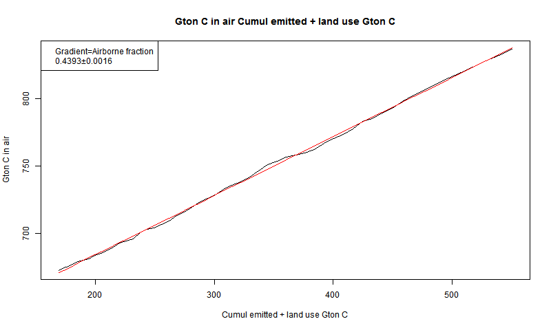
Yes it is. Here is a plot of annual (no seasonal) CO2 in air (Mauna Loa) vs cumulative emissions. Very linear (here is why).
Further to comments by Fonz and Nick, extracted from my previous posts
I have stated since January 2008 that:
“Atmospheric CO2 lags temperature by ~9 months in the modern data record and also by ~~800 years in the ice core record, on a longer time scale.”
{In my shorthand, ~ means approximately and ~~ means very approximately, or ~squared).
It is possible that the causative mechanisms for this “TemperatureLead-CO2Lag” relationship are largely similar or largely different, although I suspect that both physical processes (ocean solution/exsolution) and biological processes (photosynthesis/decay and other biological processes) play a greater or lesser role at different time scales.
All that really matters is that CO2 lags temperature at ALL measured times scales and does not lead it, which is what I understand the modern data records indicate on the multi-decadal time scale and the ice core records indicate on a much longer time scale.
This does NOT mean that temperature is the only (or even the primary) driver of increasing atmospheric CO2. Other drivers of CO2 could include deforestation, fossil fuel combustion, etc. but that does not matter for this analysis, because the ONLY signal that is apparent signal in the data is the LAG of CO2 after temperature.
It also does not mean that increasing atmospheric CO2 has no impact on global temperature; rather it means that this impact is quite small.
I conclude that temperature, at ALL measured time scales, drives CO2 much more than CO2 drives temperature.
Precedence studies are commonly employed in other fields, including science, technology and economics.
Does climate sensitivity to increasing atmospheric CO2 (“ECS” and similar parameters) actually exist in reality, and if so, how can we estimate it? The problem as I see it is that precedence analyses prove that CO2 LAGS temperature at all measured time scales*. Therefore, the impact of CO2 changes on Earth temperature (ECS) is LESS THAN the impact of temperature change on CO2 (ECO2S).
What we see in the modern data record is the Net Effect = (ECO2S minus ECS). I suspect that we have enough information to make a rational estimate to bound these numbers, and ECS will be very low. My guess is that ECS is so small as to be practically insignificant.
Regards, Allan
*References:
1. MacRae, January 2008
http://icecap.us/images/uploads/CO2vsTMacRae.pdf
Fig. 1
https://www.facebook.com/photo.php?fbid=1200189820058578&set=a.1012901982120697.1073741826.100002027142240&type=3&theater
Fig. 3
https://www.facebook.com/photo.php?fbid=1200190153391878&set=a.1012901982120697.1073741826.100002027142240&type=3&theater
2. http://www.woodfortrees.org/plot/esrl-co2/from:1979/mean:12/derivative/plot/uah5/from:1979/scale:0.22/offset:0.14
3. Humlum et al, January 2013
http://www.sciencedirect.com/science/article/pii/S0921818112001658
Buncha’ hand waving, Nick. Here is the real correlation:
http://i1136.photobucket.com/albums/n488/Bartemis/tempco2_zps55644e9e.jpg
That’s wrong Nick. First the amount of weight per cubic meter increase is really, really small. Second, the half part is really wrong. Pressure gradients, highs and lows, far out weigh any increase in the minute amount of weight. The o2 was always there. The only thing added was a carbon atom, many years less than one in a million. Third there is no way to account for no negative numbers from 1850 to 1910. The carbon cycle isnt/wasn’t that we’ll balanced. See the article just discussed on plants holding there breath. Did the structure of plants change ? I’m thinking that burning fossil fuels may have saved the planet and all life on it from carbon starvation of plants. And fourth, the current rate of sinking far outweighs any known mechanism.
You don’t see the paradox do you ? …. Finally, as far as I’m concerned, co2 follows temperature. Changing the data after I presented the evidence isn’t going to change my mind. NOAA is being high handed and capricious. It is doing a disservice to those in the far future and now for failing to acknowledge that co2 follows temperature. Of course, I believe they already knew. Those guys aren’t stupid. And they’ve known for awhile. I was carefully keeping track of it.
http://www.drroyspencer.com/wp-content/uploads/simple-co2-model-fig01.jpg
Above are the accumulation rates of both emissions and atmospheric co2. Clearly visible in the rate of atmospheric carbon growth is the temperature “fingerprint”. (of particular interest being the known step rises in temperature that occur circa 1980 and 2000) Parameters of cumulative emission graphs are as such that they do not show this variation in the growth rate. So, you can easily have two data sets that trend alike over time that look sexier in a cumulative graph then they actually are…
You are correct, Michael. Figure 2 from the article is a graph that takes the purported pre-industrial, steady state for granted. In this land of make-believe, there is no rhyme or reason for the natural balance – it just happened. Thus, they can decouple the natural from the human, and assume human impacts play out independently of nature, which is always there, reassuringly to rebound to its natural, Edenic state once the parasitical humans have exhausted their abusive proclivity.
It’s hooey. It is pre-Enlightenment primitivism, not science.
We should remember there are two sides to the equation. There is how much CO2 we put out/fossil fuels we burn every year and there is the natural absorption rate of plants, oceans and soils every year.
The natural absorption has been rising as the amount of CO2 in the atmosphere has increased. This is going to forestall the time when we reach peak CO2.
My best guess is something like 580 ppm in 2180 with this same idea that our emissions will eventually peak and decline very slowly starting sometime fairly soon, while the natural absorbers will go on increasing until it matches our emission rate and we have “peak CO2”, but that is a long way out. “Peak anything” is a very hard prediction of course since it is always wrong.
Before NOAA fixed the numbers for better science, from 2006 to 2014 the amount missing over and above the calculated absorption ranged form 4 BMT to 7.5 BMT, most were closer to 7.5. In 2014 the amount produced was 38 BMT 19 BMT was calculated to be absorbed. That left 7.5 BMT that went somewhere. Or in other words out of the 38 BMT, 26 BMT was sunk. The total amount sunk in 1965 was around 6 BMT, and the other 6 BMT made its way into the atmosphere. So whether you take an approximation of 1 ppm per 6 BMT, weight of the atmosphere, or molecular mole. The sink is 4 times what it was. So approximating that a little over 3 times as much co2 was produced, the sink would have come in at the 19 BMT mark. The sink is about 1 1/3 times higher than it should be The amount of ppm should have been over 3 and not closer to 2. In fact, 2009 it came in at 1.89. And 1998 to 1999 the amount that dropped out was 12 BMT.
These numbers weren’t variations, they were constant. I challenge your premise.
Concerning the minor amounts missing in 1965, could be through approximation, or actually significant. I’m treating it as approximation. Where did I get these numbers? NOAA.
When we run out of oil, there are still methane hydrates in vast amounts. Some estimate 10X more than crude oil energy reserves.
http://geology.com/articles/methane-hydrates/
Wang et al look at that. But they discount hydrates as not feasible in their 21Cen time frame.
Now all you have to do is find Japanese investors willing to give you $100 billion to produce hydrates. If you get it I want a gig running a hydrate extractor rig, I charge only $4000/day. That should be fun.
We have already had close to .6C warming in the 21st Century. Peak to peak in GISTEMP is about .4 (for now).
Willis, I think you need to add to the chart an analysis of the total reserves numbers. While fossil fuels were extracted, this number was increasing rather than decreasing. This makes the downturn on the production chart questionable.
MN, reported reserves are not relevant. Subject to manipulation (not least price assumptions). The ‘correct’ metric is TRR (technically recoverable reserves at any price). Now redo your homework using TRR.
Reserves bookings are guided by economics, regulations, and politics. This means the “official books” don’t carry everything we think we should be able to extract. In some cases the reserves are political, for example OPEC countries use these figures to jostle for quotas. Other countries manipulate them to improve their finances (they hope to get better (lower) bond interest rates). Companies booking under SEC regulations are forced to underbook, although that’s changed a bit in recent years, and now it’s getting better. On the other hand, some fields with shale production are a bit overbooked. It gets really really complicated.
When you talk the science we listen and learn.
I’m sure Al Gore and Leonardo DiCaprio have killer, fool-proof rebuttals to this argument ready to hand… for their next tragie-comedies. Complete with hysterical hyperbole and graphic images of snowmelt.
There simply are no good estimates of unconventional recoverable reserves. We have no idea where it will work, at what price, at what point in our technology curve. The gains made in reserves and production cost in the last two year in the Permian basin are staggering. Profitable at $25, enormous reserves. Then there is this little Russian shale:
———————————————————–
“Everything about Bazhenov is on almost unimaginable scale. It covers an area of almost 1 million square kilometres – the size of California and Texas combined.
The formation contains 18 trillion tonnes of organic matter, according to the U.S. Geological Survey (“Petroleum Geology and Resources of the West Siberian Basin”, 2003).
Bazhenov is estimated to hold more than 1.2 trillion barrels of oil, of which about 75 billion might be recoverable with current technology, making it the biggest potential shale play in the world, according to the U.S. Energy Information Administration (“Technically Recoverable Shale Oil and Shale Gas Resources”, 2013).
To put that in context, Bazhenov contains an estimated 10 times more recoverable oil than the famous Bakken formation in North Dakota and Montana.
Bazhenov could produce more oil than has so far been extracted from Ghawar – the super-giant field in Saudi Arabia that made the 20th century the age of petroleum.”
————————————————————————————
And that is just at “current technology”
The Permian basin looks pretty good. But wells aren’t viable at $25 per barrel. That’s touted by Morgan Stanley, and god knows they know very little about the business. They do wear very expensive suits.
I just looked at rate versus cumulative plots for several basins, and it sure looks like most reservoir sectors have a hard time achieving 200,000 barrels per well. Given well costs, and the hassles we have producing these crooked wells, it seems that $60 per barrel is the price needed to get things going to reverse the decline we have seen in the last two years.
The USGS figures for the Permian are guesswork. I happen to know Walter in person, and he’s a top professional, but their methods aren’t intended to be useable for official bookings. They are basic resource guidance.
The Bazhenov is large, but most of it is worthless. These shales have to have light oil with a fairly high GOR, the pressure has to be high (it helps to have an overpressured gradient), the rocks have to be brittle, and do require some sort of natural permeability (such as very small natural fractures), the geólogy has to allow for smooth drilling of long laterals, and the cost environment has to allow producing thousands of wells at very low rates (say 30 BOPD). This hurdle set isn’t met by most of the Bazhenov at $100 per barrel. We don’t really know what’s going to happen there, but from what I see thus far, Russian companies aren’t about to go nuts developing that stuff.
Please read essay Matryoshka Reserves. Everything you cite about Bahzenhov (I am not disputing that you have cited correctly) turns out not to be true. You have to drill down way deep. TOC is not a proper indicator. A large swath is autofractured and depleted; Bahzenov is the source for Siberias many conventional reservois like Samotlar. The Bahzenov stratigraphy is very unfavorable, the exact opposite of the Bakken used for comparison in the essay.
Just How Much Does 1 Degree C Cost?
https://co2islife.wordpress.com/2017/01/25/just-how-much-does-1-degree-c-cost/
The point of this thread by
David Long on January 24, 2017 at 2:47 pm:
There’s no doubt we will continue to have sufficient electricity after fossil fuels, even with today’s technology; necessity will overrule nuclear critics. The big issue is transportation fuel.
If you’re optimistic you would say we’re just one big battery breakthrough away from solving the problem.
____________________________________________
is:
If you’re optimistic you would say we’re just one big gold making breakthrough away from solving the problems of
Wall Street and Deutsche Bank,
Sigmar Gabriel and Barbara Hendricks,
Angela Merkel and Goldman Sachs.
____________________________________________
Alchemists golden green dreams of never ending veggie days.
Willis,
Our results agree closely with yours. The Right Climate Stuff research team at http://www.TheRightClimateStuff.com has made several presentations at Heartland ICCC and Texas Public Policy Foundation climate conferences in recent years with links to presentation videos and various reports provided on our website that agree closely with your conclusions.
We developed a supply-based RCP6.0 scenario with a maximum of 600 ppm CO2 in the atmosphere when all current coal, oil, and natural gas official world-wide reserves published by the US Energy Information Administration (EIA) are recovered and burned. Estimated world-wide coal reserves are the big driver. EIA estimates for coal reserves vary by a factor of 3 from low to high and we used the high value. Our “Business as Usual” RCP6.0 scenario assumes we will have a market driven transition to non-CO2 emitting fuels (I’m betting on new, safer nuclear reactors) to meet growing world-wide energy demand, as prices rise on depleting fossil fuel reserves. This transition will need to begin in about 2060.
Our RCP6.0 scenario has 585 ppm atm. CO2 concentration in 2100 and an assumption that other GHG and aerosols contribute their historical average of about 50% of atmospheric CO2 radiative forcing in 2100 to achieve 6.0 W/m^2 radiative forcing relative to 1750, as the IPCC AR5 defines and rates its RCP scenarios. Our simple, validated climate model, for GHG forcing, derived from Conservation of Power flows at the earth’s surface, is given by:
GMST(year) – GMST(1850) = TCS(1+beta){LOG[CO2(year)/CO2(1850)/LOG[2]}
where TCS stands for Transient Climate Sensitivity due to a slow rise in atm. CO2 concentration that is a similar metric to TCR and should have the same value, except TCS is verifiable with physical data and is defined for doubling atm. CO2 concentration with the actual variable rate of CO2 concentration rise since 1850. We estimate this doubling will occur in about 2080, 230 years after 1850.
beta is the somewhat uncertain fraction of CO2 radiative forcing provided by other atm. GHG and aerosols. While beta has significant uncertainty (see Lewis and Curry (2014)), primarily due to both warming and cooling effects of atmospheric aerosols, and with an aerosol concentration net cooling effect (not considering cloud feedbacks and other feedbacks that are incorporated into our definition of TCS) according to AR5 data. Based on AR5 CO2, other GHG and aerosol concentration histories since 1850, beta has an approximate value of 0.4 to 0.5.
However TCS(1+beta) = 1.8K with relatively little uncertainty, as this constant is dependent only on GMST rise since 1850 and uncertainty in CO2(1850) that we used as 284.7ppm, based on smoothed NOAA data from East Antarctica Law Dome ice cores. We used the smoothed ice core CO2 data up through 1958 and the NOAA Mauna Loa yearly average value for CO2(year) in subsequent years.
Using these numerical values for constants in the model and a tight upper bound on HadCRUT4(1850) = -0.22K, the forecasting equation can be written:
GMST(year) = -0.22 + 1.8{LOG[CO2(year)/284.7]/LOG[2]} deg K
The equation forecasts a tight upper bound on HadCRUT4 data scatter for all years except Super El Nino year weather events.
Since TCS(1+beta) = 1.8K, TCS = 1.2K if beta = 0.5 and TCS = 1.3K if beta = 0.4 that agrees closely with Lewis and Curry (2014) results for TCR and your TCR results in this article.
Using our above “climate model” that is actually only a validated GMST forecasting model, as a function of atm. GHG and aerosol concentrations, we project <1K additional GMST rise by 2100. For example our RCP6.0 scenario with CO2(2100) = 585 ppm and beta = 0.5, we obtain
GMST(2100) = HadCRUT4(2100) = -0.22 + 1.8{LOG[585/284.7]/LOG[2]} = 1.65K
HadCRUT4(2016) = 0.75 (preliminary) 1.65K – 0.75K = 0.9K additional HadCRUT4 rise by 2100.
Here in Texas, certainly one of the well explored oil territories on Earth, a 4BB oil field was found in the Permian Basin area, which is one of the most heavily explored oil regions in Texas. I say this not out of disrespect to Fernando or ristvan, but to say anecdotally what has been true since the petroleum age started: every time the peak of oil has been declared, and it has been declared several times, the declaration has been demonstrated to be incorrect.
Yup. Now figure the fracked total Permian as a percent of global production. Then get back.
There in Texas nothing new was found. I was being taught about the Wolfcamp and the Spraberry in the spring of 1978, when I was attending a geólogy for petroleum engineers course. In those days the shale section was mostly seen as source rock and something we had to understand so we could spot, drill, and complete better wells. But we knew that stuff was there.
What’s really new about those reservoirs is the ability to drill horizontal wells, fracture them, and make money. And as it turns out even today at $50 per barrel the oil price is higher than it was in the past. The other problem we have is that we simply don’t know where to turn to next. This is one reason why Permian lease sale prices are increasing so much. We are fighting like piranhas for whatever is left.
Peak oil again, so soon after its latest demonstrated failure? Finite minds can only imagine finite supplies, in direct proportion of one to the other. I expect there is a reason why we are continually treated to this silliness. Hint: what did P.T. Barnum say was “born every minute”?
Now all you have to do is point me in the right direction. Tell us, where are we supposed to look? Where will we be producing new oil reservoirs in 20 years? Any ideas?
And when we run out of coal we can start mining the hills.
I know of two railways that could be described as gravity lines, the first is the Ffestiniog Railway in Gwynedd, Wales. This line was built to carry slate from the mining town of Blaenaeu Ffestiniog to the harbour in the coastal town of Porthmadog where the slate was loaded onto ships. The line was constructed between 1833 and 1836 and was designed with a continuous 1 in 80 gradient down to the coast to permit the loaded slate trains to run by gravity for 13.5 miles from the mines to the sea.
The second is the Iron Ore Line a 247 mile long route used to transport iron ore from the mines at Kiruna in Sweden to the ice-free port of Narvik in Norway. These ore trains weigh 8,600 tonnes and use only a fifth of the electrical power they regenerate as they travel by gravity down to the coast.
So while we can use water falling under gravity to generate hydroelectric power the Iron Ore Line is an example of using rocks falling under gravity to generate lithoelectric power.
So here’s my latest Heath Robinson boondoggle:- Starting with quarries in The Himalayas, mine the rock, load it onto electrically powered wagons, run a gradient line and deliver the load to the plains generating electricity as the wagon load descends under gravity. The waste rock could then be transhipped onto barges, sent down river and used to create new land for Bangladesh and to build up their coastal levee defences.
A crazy idea? Of course it is, but a least it is green energy and after all this is what nature does every day in every sediment laden river in the world, delivering the rocks from the mountains back to the sea.
P.S. Now this scheme would really cause a rise in global sea level!
P.P.S. /sarc
WTF !
“Supply-driven projections” of MONEY more like !
Whether or not Wang is wite or wong, Wang wi-ceives the wonga.
Willis
as usual, an interesting article and whilst I do not disagree with your comments and conclusions drawn (other than I do not consider that we are running out of fossil fuel any time soon), I consider that one fundamental issue is overlooked.
I would suggest that if Governments adopt a policy aimed at mitigating climate change (rather than adapting to climate change) there has only ever been one key scientific question that needs to be answered, namely: Do any of our policies, such as the drive towards green renewable energy and putting a price on carbon (by whatever means the latter is achieved), actually reduce CO2 emissions, and if so by what extent? Thereafter it is simply a matter of politics and economics.
The inescapable fact is that our policy responses do not reduce CO2 emissions by any significant amount, and therefore one does not even need to address the Climate Sensitivity issue. If one is not materially reducing CO2 emissions, it matters little how sensitive the Climate is to CO2. We are not effectively reducing CO2 emissions save for economic activity depression such as the slow down in emerging markets. We know the following fundamental facts:
1. Wind and solar do not reduce CO2 emissions since they are intermittent and non despatchable and thereby require 100% back up by fossil powered generation.
2. Putting a price on carbon merely puts up the price at which the finished goods are sold; it does not take away demand, and hence does not reduce CO2 emissions.
3. Placing impediments on carbon trading, merely results in industry relocating from one geographical location to another and hence globally does nothing to reduce CO2 emissions.
With present day technology there are only a few options that could dramatically reduce our CO2 emissions, namely to go nuclear, or hydro and geothermal where geography/topography opens up such opportunities. But no Government is going down that road.
Switching from coal to gas, is partial decarbonisation, and we know that this works better than wind and solar; compare US emissions with Germany’s emissions these past 15 or so years. Fracking is obviously a sensible policy as a half way house, but again, apart from the US, no major Government is yet going down that route.
Just like the stoneage did not come to an end due to our running out of stones, the fossil fuel age will not come to an end due to our running out of fossil fuel. It will only come to an end when a cheaper and more abundant energy source opens up. The dawning of a new energy era will not be wind and solar, but will be some form of technological breakthrough probably with nuclear (whether fission or fusion) but possibly with solar located in space and beamed back to Earth.
As most politicians realise, it is the economy stupid. The economic realities are beginning to roost. Trump is a business man and he can see the farce of the present policies (prohibitively expensive, job destroying and achieving no worthwhile reduction in CO2). Much of the developed world is in near economic stagnation, and the costs of this fiasco are beginning to dawn as it is appreciated that the developed world will not get out of the economic doldrums whilst so heavily shackled by green policies. The US will lead the way, the rest of the world will follow some time later.
In the meantime, the climate will do whatever the climate chooses to do.
I agree with that mostly, except for wind and solar not reducing CO2 emissions due to need for 100% fossil fuel backup. Wind and solar will reduce CO2 emissions during the times when they can make use of wind and sunshine. Also, increasing price will cause a reduction of demand – what to argue there is how little, not that the reduction is zero.
I blame this on Global Hillary Warming
Then and now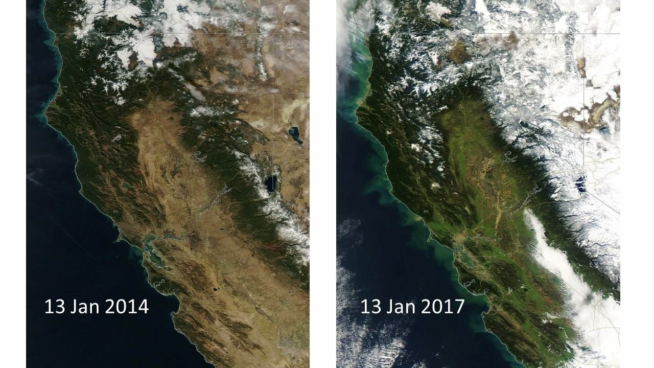
Wasn’t climate change going to bring never ending droughts.
Yet another failed prediction.
The problem is that the world’s oil and gas resources are much more limited than the coal reserves.
Moreover, coal is in every respect the most polluting of the tree.
If we see a supply driven peak in oil or gas, we may have to replace that with coal.
This will increase several kinds of emissions including the carbon emissions. It gives more methane, more particulates, more SO2, more heavy metals, and more CO2 per energy equivalent.
/Jan
Here’s a link to work by Steve Mohr on coal resources
http://www.theoildrum.com/node/5256
Regarding: “If we want to see what temperature change we can theoretically expect during the 21st century from the possible atmospheric CO2 scenarios shown in Figure 2, obviously the value to use is the TCR”, and the Figure 3 boxplot:
To get .8 degree C temperature rise using 633 PPMV CO2 and 1.8 degree C per 2XCO2, I figure the 633 PPMV is an increase by a factor of 2^(.8/1.8) or 1.361. The effect of CO2 is generally considered as logarithmic. Log(1.361)/log(2) – .8/1.8. Meanwhile, 633 PPMV / 1.361 is 465 PPMV. So, a high side transient climate response of .8 degree C is not all of the (high side) warming to occur this century. This gets added to the warming resulting from increasing CO2 to 465 PPMV.
A more realistic high side warming this century using 1.8 degree C per 2X CO2 high side TCR and 633 PPMV as high side CO2 considers the CO2 increase to 633 PPMV during the preceding 70 years, which looks to me as being from 2005 to 2075 according to the Figure 2/5 graph. 2005 CO2 was about 379 PPMV. Log(633/379)/log(2) is .74. That times 1.8 is 1.33 degree C warming from 2005 to 2075. Although the few years centered around 2005 had global temperature being boosted about .1-.11 degree C by AMO and maybe other multidecadal oscillations, the amount of warming “still in the pipeline” from CO2 increasing to 379 PPMV was probably at least that much, leaving 1.33 degree C intact as a high side warming from 2005 to 2075.
And the warming won’t stop in 2075 but merely slow down using this scenario. The 633-PPMV-peaking curve in the Figure 2/3 graph is down only to slightly above 580 PPMV at the end of the century. Using that and high-side ECS of 3.1 degree C per 2XCO2 (according to “with the transient climate response (TCR) now re-estimated at 1.8 °C per doubling of CO2 (ECS increases to 3.1 °C/2xCO2)”): 3.1 x log(580/379)/log(2) means 1.9 degree C warming. Since this exceeds 1.33 degree C, high-side means warming will continue from 1.33 degree C in 2075 to somewhere between 1.33 and 1.9 degree C (although probably closer to 1.33 degree C) in 2100.
I follow this up using middle-of-the-road figures of 519 PPMV according to the Figure 3 boxcar plot and TCR of 1.3 degree C per 2XCO2:
It looks to me that a good choice of year for CO2 to be 519 PPMV is 2070. 70 years before that is 2000, when CO2 was about 371 PPMV. Log(519/371) / log(2) x 1.3 is .48 degree C warming from 2000 to 2070, and in this scenario the warming won’t stop but merely slow down around 2070.
The .3 degree C figure shown in the Figure 3 boxcar plot using TCR of 1.3 degree C per 2XCO2 and 519 PPMV CO2 means 519 is an increase by a factor of 2^(.3/1.3) or from 442 PPMV. Log(519/442) / log(2) x 1.3 = .3.