Guest Post by Willis Eschenbach
I’ve been investigating the use of the “complete ensemble empirical mode decomposition” (CEEMD) analysis method, which I discussed in a previous post entitled Noise-Assisted Data Analysis.
One of the big insights leading to modern signal analysis was the brilliant idea of Joseph Fourier. He realized that any given waveform can be expressed as a combination of sine and cosine waves. However, there are other ways besides Fourier’s method to decompose a signal, including periodicity analysis, principal component analysis, and CEEMD.
Let me give you an example of a CEEMD analysis. Here are the intrinsic modes for the annual average number of sunspots from 1700 to 2014. The top row is the sunspot data itself. For intercomparison with other signals, it is standardized to a mean of zero and a standard deviation of one.

Figure 1. CEEMD analysis of the mean annual sunspot numbers. Top panel shows the sunspot data, standardized to a mean of zero and a standard deviation of one. Panels marked C1 – C7 show the intrinsic modes of the signal. The bottom line shows the residual, meaning what remains after the removal of modes C1 – C7 from the signal. Note that all intrinsic modes are displayed at their true size, with all scales being the same.
This is a “complete decomposition” of the raw data signal, meaning that if we add the intrinsic modes C1-C7 together plus the residual, it will faithfully and exactly reconstruct the original signal.
One thing I like a lot about the CEEMD analysis is that I can actually see how the underlying intrinsic modes vary over time. I’ve said before that ascribing an inherent cyclical mechanism to natural observations is fraught with problems. Figure 1 is a good example of these problems. Look at intrinsic mode C4. It has a small signal at about 22 years … but not all of the time. For most of the first century of the record there is little signal at all. Then there’s an intermittent small ~ 22-year signal from about 1780 to 1850 ,,, which fades out and after a few year hiatus is replaced by a single ~ 25-year cycle, and that in turn is replaced with a ~ 22-year cycle out to the end of the data.
Or we can consider intrinsic mode C6, which varies in a similar irregular fashion. Mode C6 has a couple of strong cycles with a period of around 90 years at about 1800, and it then kind of tails off to nothingness. This makes it obvious why it has been so hard to discuss the existence or non-existence of the so-called “Gleissberg Cycle”, which Gleissberg claimed was ~ 80 – 100 years. When cycles come and go like that, it is hard to draw any firm conclusions. I mean, the ~ 80 – 100 year cycle is definitely there … but it’s only there when it is there, and the rest of the time, well, it’s simply not there.
Unfortunately, these kinds of appearing and disappearing cycles are far too common in natural datasets. There is a great temptation to think that they can be used for forecasting purposes … and they could if we ignore Murphy’s Law, which says that as soon as you start prophesying, the cycle will die out. For example, if we looked at the sunspot data in the year 1900, we’d think that there was a strong, statistically significant hundred-year cycle in the data … but after 1900 the cycle simply fades out to nothing.
Having seen the actual waveforms of the intrinsic modes in Figure 2, we can look at the periodograms of the various intrinsic modes to see what kind of signals exist in each of the intrinsic modes C1 to C7.

Figure 2. Periodograms of each of the intrinsic modes C1 through C7 of the annual mean sunspot number, 1700-2014. These show the strength of waves of the various periods in each on the intrinsic modes.
Figure 2 shows that most of the energy is in the ~11 year cycle, which is in intrinsic mode C3. Because the sunspot cycle varies between ten and thirteen years, the energy is not a sharp spike, but has energy across that range.
As discussed above, intrinsic mode C4 can be seen to have a very small bit of energy in the 22 year range, but as we saw in Figure 1, there’s nothing regular enough in the data to give a strong signal.
Again as discussed above, intrinsic mode C6 seems to have some energy in the 90-100 year range … but as Figure 1 shows, the ~100 year signal in C6, while strong, is mostly visible in the first half of the data. This greatly increases the odds that it is a spurious signal that could disappear in a longer record.
So that is an example of a CEEMD analysis of a signal. It gives us a picture of the intrinsic modes (Figure 1) and the periodograms of those same intrinsic modes (Figure 2). It shows the strength and the ebb and flow of the underlying cycles in the data.
Now, how else can this kind of analysis be useful? Well, it can show whether and how two distinct observational datasets might be related. As an example, here is the CEEMD analysis of both the Nino3.4 Index and the Southern Ocean Index (SOI). The Nino3.4 Index is a detrended sea surface temperature dataset for an area in the tropical central Pacific covering 5° North to 5° South and 120° West to 170° West. The SOI, on the other hand, is an index of the atmospheric pressure difference between Tahiti and Darwin, Australia. The two indexes seem to be measures of the El Nino/La Nina pumping action. The SOI and the Nino3.4 move in opposite directions, so the SOI is usually displayed inverted so that peaks in the SOI correspond with peaks in temperature. The next two figures show the CEEMD analysis of the two datasets:


Figures 3 and 4. Upper figure shows the intrinsic modes resulting from the CEEMD analysis of the Southern Ocean Index (SOI, red) and the Nino3.4 Index (black). These two datasets cover the same period as the sunspot data shown in Figure 1, 1870 – 2011.
Again, we see that there are various cycles which are strong in part of the record, but disappear or are greatly diminished in other parts of the record.
Note the close correspondence of the decomposition of the two signals, both in terms of the strength and shape of the intrinsic modes, and in their periodograms. It is clear that regardless of the fact that the Nino3.4 Index and the Southern Ocean Index are measuring different variables, they are both a measure of the same phenomenon.
And it is equally clear that there is no significant sunspot signal in either the SOI or the Nino3.4 data—the CEEMD analysis shows little commonality. Unlike the sunspot data, in the SOI and Nino3.4 data there is little strength at 11 years, and little strength at around 90 years. And again unlike the sunspots data, the majority of the energy is in the short-cycle (2-6 year) part of the spectrum.
Anyhow, that’s why I’ve grown fond of the CEEMD analysis … it shows when datasets have related cycles, and when they are unrelated.
Pushing towards full moon tonight, with Jupiter and Arcturus vying for the moon’s attention … what a world …
My best to everyone,
w.
My Usual Request: Misunderstandings bring communication to a halt, so if you disagree with me or anyone, please quote the exact words you disagree with so we can all understand your objections. I can defend my own words. I cannot defend someone else’s interpretation of some unidentified words of mine.
My Other Request: If you believe that e.g. I’m using the wrong method or the wrong dataset, please educate me and others by demonstrating the proper use of the right method or the right dataset. Simply claiming I’m doing something wrong doesn’t advance the discussion unless you can tell us how to do it right.
Yearly Sunspot Data: SILSO
SOI Data: Here
Nino3.4 Data: NOAA
Code: I’m using the “CEEMD” function in the R package “hht” for the analysis.
As the coronal hole rotates rigidly. I repeat rotates rigidly, observations indicate that what cause/creates the coronal hole must come from the solar interior, not the solar convection zone
I discovered that back in the early 1970s, so this is old news. And already back then it was clear that the origin of rigid rotation was to be sought at depth. As Gough points out in http://www.leif.org/EOS/1505-04881-Gough-Helioseismology.pdf ”
“it is interesting that the sector structure of the solar wind, which might mirror the magnetic asymmetry within the Sun, has maintained its phase for at least four sunspot cycles prior to the mid seventies (Svalgaard and Wilcox 1975). Further, similar, analysis of solar-wind data up to the present day would therefore be very welcome, and could add (or subtract) credence to the hypothesis [of an internal relic magnetic field].
The cumulative/magnification issue reminds me of the tides. So let’s apply that proposed mechanism to tides. If one were to only add the strength of high tides above some kind of anomaly baseline mean, and then say the tides beyond that accumulate energy, pretty soon the East Coast tide coming in will meet the West Coast tide going out. Which is absurd.
However, keep this under your hat. It could very well be picked up by some AGWarming scientist who then writes a grant to determine if this could happen, do the study, and then publish the damnable thing!
Willis, thank you as always for a very informative article. I note in your closing comments that you’re using the Hilbert-Huang Transform (hht) tools and methods in R.
I’ve done time series modeling and biostatistics using a C# wrapper to the R engine when I have unique and complex analyses to perform. I haven’t delved into CEEMD but would like to investigate it for other uses in my field. Thanks for showing its possibilities.
“George E Smith commented: ””””….. like natural warming and cooling trends in the oceans regulated by their circulation and their ability to move warmer water to the north where it radiates to space more easily. …..”””””
Nothing could be further from the truth.
“Thermal” (BB like) electromagnetic radiation radiance varies as the 4th power of Temperature, so the very last thing that is going to happen to energy in warmer waters that move north, will be increased radiation to space.
The VERY HOTTEST tropical (high) deserts in the middle of the hottest summer days, is where you should look for efficient cooling of the earth; at rates almost twice that for the global nominal 288 K Temperature, but the very coldest places like the Antarctic highlands or the northern polar regions, can only radiate at rates as low as one sixth of the global mean rate.
The polar regions DO NOT COOL THE EARTH.
We need here to consider heat flow and reservoirs – the hot deserts cool down at night very quickly as there is no transfer of heat from below – whereas as the oceans lose heat at the surface they are subject to a heat-exchange effect from currents – for example, the zones of maximum heat transfer from ocean to atmosphere and hence to space occur along the western boundary currents in the Northern Hemisphere. The heat flow from oceans to space is modulated by cloud cover, and there are cloud bands that insulate in both the southern and northern hemisphere – any movement north or south of these bands, or variability in percentage cover will affect the heat transfer. Apart from the incursion of warm water into the Norwegian and Barents Seas, where there is no great transfer compared to the western boundary of the Atlantic and Pacific, most of the heat loss is occurring below 60N and 60S. I suspect that cyclones extract significant heat – creating cloud banks, and the pattern of cyclonic activity varies over time – with either the variable jetstream (modulated by solar UV) being causal (or consequent, if the variability is internally driven).
“Mode C6 has a couple of strong cycles with a period of around 90 years at about 1800, and it then kind of tails off to nothingness. This makes it obvious why it has been so hard to discuss the existence or non-existence of the so-called “Gleissberg Cycle”, which Gleissberg claimed was ~ 80 – 100 years. When cycles come and go like that, it is hard to draw any firm conclusions. I mean, the ~ 80 – 100 year cycle is definitely there … but it’s only there when it is there, and the rest of the time, well, it’s simply not there.”
Events wander from the mean intervals, we already know that from solar minima, the Dalton Minimum was from SC5, the Gleissberg Minimum from SC12, and the current minimum from SC24, so there’s no point in expecting a fixed periodicity.
“And it is equally clear that there is no significant sunspot signal in either the SOI or the Nino3.4 data—the CEEMD analysis shows little commonality.”
The majority of solar cycles have an El Nino episode or conditions around a year after sunspot minimum. The weakest solar magnetic phase of the Dalton Minimum 1807-1817 saw roughly a doubling of El Nino episode frequency:
https://sites.google.com/site/medievalwarmperiod/Home/historic-el-nino-events
“The majority of solar cycles have an El Nino episode or conditions around a year after sunspot minimum. – Ulric” Yes sir!
If you compute, plot, and overlay the rate of annual PMOD change over top of HadSST3, you can see as the rate of TSI change ramps up at the onset of a solar cycle, SSTs ramp up, creating an El Nino. It’s evidence for ‘solar supersensitivity’.
The SUN causes El Ninos from either the rapid onset of higher TSI at the start of a solar cycle, or at and after the solar maximum TSI peak(s). The duration of solar max El Ninos is exclusively dependent on the strength and duration of the preceding TSI, and the solar min El Ninos are dependent on the timing and duration of a rising rate of increase of TSI, producing a La Nina when the rate becomes negative.
http://www.esrl.noaa.gov/psd/enso/mei/ts.gif
1955 was a solar minimum La Nina year, followed by the SC19 peak pre-1960, then the low and choppy SC20 with many La Ninas, then more frequent/longer duration El Ninos during the higher TSI cycles SC21-23, then a return to more frequent La Ninas during the long low solar minimum pre-SC24, and then the most recent upswing from the most recent solar cycle, with both the new cycle fast-rising-TSI ENSO in 09/10, and the post-TSI maximum ENSO in 2015.
Gavin Schmidt predicted another record year for 2016. Since January I have consistently predicted lower temps for this year from lower TSI this year.
With 21 El Ninos since 1950 and less than four solar cycles it is not hard to find El Ninos wherever you want them, so your associations are not different from throwing dart at the chart.
Bob Weber April 22, 2016 at 9:42 am Edit
Thanks, Bob. Do you truly believe this? And why? It appears you haven’t done even the most simple of statistical analyses. Take the MEI and check the correlation with sunspots, and report back to us … be sure to include autocorrelation in your statistical analysis.

I would venture to say, without even doing the exercise, that your results will NOT be statistically significant … but I’m happy to be proven wrong.
…
…
OK, I just ran the numbers to save you the work. Here’s the scatterplot:
The p-value is a ludicrous 0.38, and with optimum lag (six months) it reduces to a still ludicrous 0.32 … sorry, amigo, but your theory just ran into a reef of facts.
w.
Use PMOD, not sunspots. Sunspot numbers are not energy.
You don’t know what you’re looking at until you look. Did you make an annual rate of TSI change plot as I suggested to Willis and Ulric and overlay it over HadSST3? If you can’t bring yourself to do that then your complaints are moot.
Willis you are very famous for asking people to stick to what people say. In this blog post I have repeatedly implored to not use sunspot numbers in lieu of TSI, but you went ahead and used sunspot numbers anyway, making your statistical example misleading as it doesn’t represent the actual real solar energy in time or magnitude. Are you going to dispute that?
Do you not realize from my earlier comments that TSI lags sunspot numbers and solar flux? So your choice to use sunspot numbers instead of TSI was a deliberate choice to ignore that fact and of course will by default produce statistical crap.
If you have not created the rate of annual TSI change plot like I suggested to you earlier, then you have no idea what you are talking about, because you wouldn’t know what I was talking about. You keep carrying on like you know something real about TSI from your scatterplot – you’re going to look very foolish after I produce my own plot. You’re way out there on a limb on this and you don’t realize it.
The step change in SST some say came from the 1998 ENSO did not come from that ENSO, as the La Nina had already discharged that heat prior to 1999.
The step change came from the high TSI at the end of the modern maximum in solar activity, where 7 of the top 11 PMOD TSI years occurred after 1990, with 4 of the top ten 1999-2002, providing the energy for the decent step change in SSTs into the early 2000’s, only to be eclipsed by the recent TSI-driven ENSO.
Another confirmation of my TSI predictions is already underway. I’ve told you before that when TSI goes up, tropical evaporation goes up, heavy vapor plumes enter the US, we get floods, wind, hail, and tornadoes. It’s happening again. Tornadoes dropped by 70% in April, according to Dr. Greg Forbes of The Weather Channel, and that’s no surprise to me since TSI dropped through most of the month.
The tail end of that periods’ precipitation just cleared out this morning – only 2 hail reports and no tornadoes yesterday, just in time for all new evaporation and weather events. TWC is predicting higher torcon numbers next week, right on cue, as TSI just turned the corner and is going upwards again as of last weeks data (today’s TSI is from one week ago), and the water vapor is streaming in now after dropping off considerably for weeks.
Willis, I do know what is going on, what did go on, and I can predict what will go on based on what the sun’s TSI is doing, partly because I have over 100 data sets in 270 MB spread out over six workbooks with regularly updating data. One of those is an extreme events sheet with all the SPC storm reports complied together and up to date since 1950, including wind, hail, and tornadoes, which I’ve plotted out against TSI over the past 13 years, and along with hurricanes and typhoons. In most cases extreme events occur on or after the rising phase of TSI during a solar rotation, and preferentially when TSI is high. It’s all in the data and at this time I’m cataloging everything one year at a time – it’s a lot of work. It’s just been great to see it happen repeatedly since I first discovered the phenomenon in January this year.
This should become your new best friend if you really want to know what you’re talking about:
http://lasp.colorado.edu/data/sorce/total_solar_irradiance_plots/images/tim_level3_tsi_24hour_3month_640x480.png
Looking forward to your usually sarcastic dismissive but sometimes funny reply.
I don’t know why but the SORCE image shown isn’t from today’s plot. The plot posted is dated through March 29. The one in my browser tab from today that I thought I was posting is dated April 15, so the big drop in TSI since then isn’t shown, strangely. TSI dipped to between 1360.0 and 1360.5 in the one I’m seeing – solar min levels!
ulriclyons April 22, 2016 at 4:43 am
Ulric, I fear you haven’t done your sums. In your cited data, you list a total of 23 El Nino events in the 20th century, each of which covers two years. So from the start, you list 46 El Nino years, or almost half of the years of the 20th as having an El Nino episode.
During the same 20th century there were 10 sunspot minima.
This means that yes, you will have an El Nino “El Nino episode or conditions” a year after sunspot minima, and a year before the minima, and during the minima … in fact, for every sunspot cycle you have almost five El Nino events, so yes, you’ll definitely find them scattered around.
However, of the ten sunspot minima listed:
7 of them happened DURING an El Nino event (according to your data)
2 of them happened BETWEEN an El Nino event ending the previous year and an El Nino event starting the following year.
Only 1 of the sunspot minima happened BEFORE an El Nino event, as you have claimed
In addition, the other 13 El Ninos had no relationship to the sunspots … well, in fact none of any of the El Nino events appear to have a relation to the sunspots, but the other 13 didn’t happen anywhere near the minimum.
In other words … as Leif said, you’re just throwing darts at the chart.
w.
“Ulric, I fear you haven’t done your sums. In your cited data, you list a total of 23 El Nino events in the 20th century, each of which covers two years. So from the start, you list 46 El Nino years, or almost half of the years of the 20th as having an El Nino episode.”
The 19th century El Nino are listed too, I didn’t list anything. Now you may like to claim that each El Nino covers two years, but in reality they can be as short as five months.
“..in fact, for every sunspot cycle you have almost five El Nino events, so yes, you’ll definitely find them scattered around.”
You haven’t done your sums, 10 solar cycles and 23 El Nino events is 2.3 El Nino events per solar cycle on average.
“However, of the ten sunspot minima listed:
7 of them happened DURING an El Nino event (according to your data)”
Possibly at the sunspot minimum at 1913.6, and also 1986.8, with both minima being very early in the El Nino which strengthened strongly through the following year or more. That’s all I can see, your 7 must be a spurious result of your two year long El Nino.
“2 of them happened BETWEEN an El Nino event ending the previous year and an El Nino event starting the following year.”
Immaterial.
“Only 1 of the sunspot minima happened BEFORE an El Nino event, as you have claimed.”
Nonsense, only one wasn’t followed by El Nino conditions or episode, after sunspot minimum 1954.3: http://www.cpc.noaa.gov/products/analysis_monitoring/ensostuff/ensoyears.shtml
“In addition, the other 13 El Ninos had no relationship to the sunspots”
It’s not the sunspots, it’s weak solar wind periods, and where that happens at sunspot maximum as it does in some solar cycles, there will typically be El Nino episodes or conditions there also.
“..in fact, for every sunspot cycle you have almost five El Nino events..”
No just in much weaker solar magnetic phases like 1807-1817:
https://sites.google.com/site/medievalwarmperiod/Home/historic-el-nino-events
1914 SOI:
https://www.longpaddock.qld.gov.au/products/australiasvariableclimate/ensoyearclassification.html
Let’s try this TCTE plot and see if it’ll be from today – it is offset higher than SORCE, and appears to be slightly more sensitive when compared directly with SORCE:
http://lasp.colorado.edu/data/tcte/total_solar_irradiance_plots/tim_level3_tsi_24hour_3month_640x480.png
Bob, El Nino behaves as a negative feedback to major slower solar wind periods, that’s why El Nino episodes increase in frequency during the weakest phases of solar minima, e.g. 1807-1817, page 11: http://www.leif.org/EOS/92RG01571-Aurorae.pdf
Thanks for the post, Willis.
And thanks, Leif, for your comments.
Cheers.
Well after all this entertaining discussion I thought it would be helpful to y’all to point out that it is straightforwad to forecast the future climate trends with likely reasonably useful accuracy.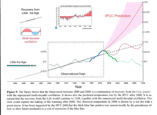
See Fig 1 at
http://climatesense-norpag.blogspot.com/2016/03/the-imminent-collapse-of-cagw-delusion.html
Fig1 (Amended ( Green Line Added) from Syun-Ichi Akasofu) http://www.scirp.org/journal/PaperInformation.aspx?paperID=3217
Figure 1 above compares the IPCC forecast with the Akasofu paper forecast and with the simple but most economic working hypothesis of this post (green line) that the peak at about 2003 is the most recent peak in the millennial cycle so obvious in the temperature data.The data also shows that the well documented 60 year temperature cycle coincidentally peaks at about the same time.
The temperature projections of the IPCC – UK Met office models and all the impact studies which derive from them have no solid foundation in empirical science being derived from inherently useless and specifically structurally flawed models. They provide no basis for the discussion of future climate trends and represent an enormous waste of time and money. As a foundation for Governmental climate and energy policy their forecasts are already seen to be grossly in error and are therefore worse than useless.
A new forecasting paradigm needs to be adopted.
Here are the latest forecasts and conclusions
“3.Forecasts
3.1 Long Term .
I am a firm believer in the value of Ockham’s razor thus the simplest working hypothesis based on the weight of all the data is that the millennial temperature cycle peaked at about 2003 and that the general trends from 990 – 2003 seen in Fig 4 will repeat from 2003-3016 with the depths of the next LIA at about 2640.
3.2 Medium Term.
Looking at the shorter 60+/- year wavelengths the simplest hypothesis is that the cooling trend from 2003 forward will simply be a mirror image of the rising trend. This is illustrated by the green curve in Fig,1.which shows cooling until 2038 ,slight warming to 2073, then cooling to the end of the century.
3.3 Current Trends
The cooling trend from the millennial peak at 2003 is illustrated in blue in Fig 5. From 2015 on,the decadal cooling trend is obscured by the current El Nino. The El Nino peaked in March 2016. Thereafter during 2017 – 2019 we might reasonably expect a cooling at least as great as that seen during the 1998 El Nino decline in Fig 5 – about 0.9 C
It is worth noting that the increase in the neutron count in 2007 seen in Fig 8 indicated a possible solar regime change which might produce an unexpectedly sharp decline in RSS temperatures 12 years later – 2019 +/- to levels significantly below the blue trend line in Fig 5.
4.Conclusions.
To the detriment of the reputation of science in general, establishment climate scientists made two egregious errors of judgment in their method of approach to climate forecasting and thus in their advice to policy makers in successive SPMs. First, they based their analyses on inherently untestable and specifically structurally flawed models which included many questionable assumptions. Second they totally ignored the natural, solar driven , millennial and multi-decadal quasi-cycles. Unless we know where we are with regard to and then incorporate the phase of the millennial cycle in particular, useful forecasting is simply impossible.
It is fashionable in establishment climate circles to present climate forecasting as a “wicked” problem.I would by contrast contend that by adopting the appropriate time scale and method for analysis it becomes entirely tractable so that commonsense working hypotheses with sufficient likely accuracy and chances of success to guide policy can be formulated.
If the real outcomes follow the near term forecasts in para 3.3 above I suggest that the establishment position is untenable past 2020.This is imminent in climate terms. The essential point of this post is that the 2003 peak in Fig 1 marks a millennial peak which is totally ignored in all the IPCC projections.”
PS For Leif – I’m sure that you regard all the above as idle speculation. From my viewpoint your approach is that of someone looking at a large pointilist painting from about 6 inches away.
Better than to look at from a mile away.
I was waiting for the last of the usual suspects to show up and peddle their pseudo-science. You did not disappoint.
about your ‘idle speculation’ as you call it, I’ll say with Tweedledee:
‘if it was so, it might be; and if it were so, it would be; but as it isn’t, it ain’t’
In fact, the pink IPCC projection looks like a much better fit to the blue curve than Akasofu’s green curve.
Dr Norman Page April 22, 2016 at 9:30 am Edit
Oh, sure, forecasting the future evolution of one of the more complex systems on the planet is “straightforward” and can be done with “reasonably useful accuracy” … riiiiiight … the mere fact that nobody has EVER been able to forecast the future climate it doesn’t stop the good Doctor.
Like the man said, if you’re so smart, why ain’t you rich? Anyone who could actually “forecast the future climate trends with likely reasonably useful accuracy” like you claim you can do would be able to make millions off it, farmers and city planners and hedge fund managers would be sitting at your feet waiting for the words of wisdom …
w.
Somehow it strikes me that goes for all the other ones who who peddle their wisdom…
Willis .
A review of candidate proxy data reconstructions and the historical record of climate during the last 2000 years suggests that, at this time, the most useful reconstruction for identifying N H temperature trends in the latest important millennial cycle may be that of Christiansen and Ljungqvist 2012 (Fig 5) Fig 9 here: http://www.clim-past.net/8/765/2012/cp-8-765-2012.pdf
The principal components of climate change of interest on human time scales are embraced in the millennial and 60 year cycles . The amplitude of the former is about 1.8 and the latter about 0.3.See Figs 9 and 15 at http://climatesense-norpag.blogspot.com/2014/07/climate-forecasting-methods-and-cooling.html
http://2.bp.blogspot.com/-4nY2wr6L-WY/U81v9OzFkfI/AAAAAAAAATM/NA6lV86_Mx4/s1600/fig5.jpg
The amplitude of the millennial cycle is taken from the 50 year moving average. The cycle is asymmetric with a downslope of about 650 years or on average 0.0028/year. Also note the amplitude of the variability about the moving average.
Here is what I say re our ability to “prove” future trends. See
http://climatesense-norpag.blogspot.com/2015/08/the-epistemology-of-climate-forecasting.html
“Ava asks – the blue line is almost flat. – When will we know for sure that we are on the down slope of the thousand year cycle and heading towards another Little Ice Age.
Grandpa says- I’m glad to see that you have developed an early interest in Epistemology. Remember ,I mentioned the 60 year cycle, well, the data shows that the temperature peak in 2003 was close to a peak in both that cycle and the 1000 year cycle. If we are now entering the downslope of the 1000 year cycle then the next peak in the 60 year cycle at about 2063 should be lower than the 2003 peak and the next 60 year peak after that at about 2123 should be lower again, so, by that time ,if the peak is lower, we will be pretty sure that we are on our way to the next little ice age.
That is a long time to wait, but we will get some useful clues a long time before that. Look again at the red curve in Fig 3 – you can see that from the beginning of 2007 to the end of 2009 solar activity dropped to the lowest it has been for a long time. Remember the 12 year delay between the 1991 solar activity peak and the 2003 temperature trend break. , if there is a similar delay in the response to lower solar activity , earth should see a cold spell from 2019 to 2021 when you will be in Middle School.
It should also be noticeably cooler at the coolest part of the 60 year cycle – halfway through the present 60 year cycle at about 2033.
We can watch for these things to happen but meanwhile keep in mind that the overall cyclic trends can be disturbed for a time in some years by the El Nino weather patterns in the Pacific and the associated high temperatures that we see in for example 1998 ,2010 and especially from 2015 on.
Fig 4”
Willis this is the nature of the beast and about as good as we can do. The main take away is the if my 2020 forecast is in the ball park the establishment forecast must of necessity surely be seen as in need of serious re-assessment.
Here is the reason I’m not rich.
“In the Novum Organum (the new instrumentality for the acquisition of knowledge) Francis Bacon classified the intellectual fallacies of his time under four headings which he called idols. The fourth of these were described as :
Idols of the Theater are those which are due to sophistry and false learning. These idols are built up in the field of theology, philosophy, and science, and because they are defended by learned groups are accepted without question by the masses. When false philosophies have been cultivated and have attained a wide sphere of dominion in the world of the intellect they are no longer questioned. False superstructures are raised on false foundations, and in the end systems barren of merit parade their grandeur on the stage of the world.”
Climate science has fallen victim to this fourth type of idol.
http://www.sirbacon.org/links/4idols.
Dr Norman Page April 22, 2016 at 12:44 pm
Dr. Page, since Christiansen and Ljunqvist never archived either their code or their data, I fear that their “study” is nothing but useless anecdote—pretty-appearing anecdote, perhaps even impressive anecdote, but anecdote nonetheless.
Anyone using it is either clueless about the study, or is knowingly using anecdotal unverifiable claims … which category are you in?
w.
Willis. Reading the details of the Christiansen paper methods persuades me that it gives a usable representation of reality’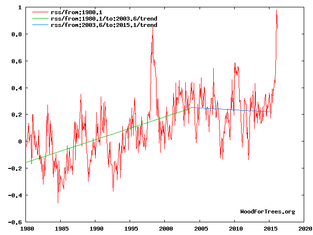
The essential point of the post is that the 2003 peak in Fig 1 marks a millennial peak which is totally ignored in all the IPCC projections.”
Here is a close up look
The El Nino peaks are temporary aberrations which can be ignored when analyzing trends.
No doubt the coincidence of the millennial peak at 2003+/- with the peaks in Evaporative Cooling and Temperature in Figs 5 and 6 at
htps://wattsupwiththat.com/2015/11/11/tropical-evaporative-cooling/
are entirely accidental unless some genius could think up a mechanism.
Link should be https://wattsupwiththat.com/2015/11/11/tropical-evaporative-cooling/
lsvalgaard April 22, 2016 at 10:25 am
Hmmm, not much unlike this event:
I quoted to someone the CAGW theory that one molecule of CO2 warms up by whole 1C each of the neighbouring 2,500 molecules of air and still stays at the same temperature,, in response he threw the same ‘fool me’ quote back at me.
How apt.
I suspect that your assertion that the every 100 extra CO2 ppm would account for 0.5C of warming would fall into same category.
every 100 extra CO2 ppm would account for 0.5C of warming would fall into same category
As you always say: I just follow the data, and that is what they show. Right or wrong? You decide for yourself based on your own bias.
But you are silent about the change of explanation for your idea about LOD. Prudent of you.
As I said you invented that, and asked you to find a quote, or admit you told a ‘porky’, you dismally failed.
What I wrote in 2014 is here
https://hal.archives-ouvertes.fr/hal-01071375v2/document
see page 3
Discussion
…….
“At the current state of knowledge, the most realistic alternative is the indirect solar effect, whereby a possible mechanism could be postulated along line:
Solar activity – ocean & atmospheric temperatures – oceanic and atmospheric circulation – angular momentum exchange – Earth’s rate of rotation (LOD) – secular change in perceived geomagnetic field.”
This is what I wrote few minutes ago:
Despite all the obfuscations the most likely scenario is:
”Solar activity has an effect on ocean & atmospheric temperatures and circulation which in turn via the angular momentum exchange affects the Earth’s rate of rotation (LOD).”
https://wattsupwiththat.com/2016/04/20/ceemd-and-sunspots/comment-page-1/#comment-2196753
you told a ‘porky’ you can’t find a quote to support it.
Considering your age and your past achievements in advancing solar science, I am happy to let you get away with it.
Over to you, let’s have another laugh.
Already in 2014 you had changed your explanation. Look back through earlier posts on WUWT [or elsewhere if applicable] and you’ll surely find where you where pushing the penetration of the solar field to the core and my debunking of it. Where would you otherwise find “that none of the solar magnetic energy can penetrate deep enough to alter the core’s angular momentum (CAM)”. So, go look, don’t be shy, and try to be honest.
No doc you got it wrong, I never claimed what you say.
You confusing two totally different things. I wrote or claimed number of times existence of a possible link between earthquakes and geomagnetic storms, due to telluric currents induction in the lithosphere affecting weak tectonic junctures
http://www.vukcevic.talktalk.net/TF.jpg
I am happy to let you off on this one, even you can make a mistake.
But I’ll not let you off. Honesty has never been a strong side of your nature. My objection that you referred to was specifically directed at your claim in the past that the solar field penetrated into the core. I don’t think you could have come up with that objection on your own. It is OK for you to change your mind [especially away from your ludicrous first idea], but it is not OK to be dishonest about it and hoping I would not notice.
Dr. Svalgaard
Insults I do not do.
Find a quote and come back.
Fair enough in anyone’s book.
Telling you how it is should not be construed as an insult. If you are interested find the quote yourself. You are better positioned to do that, and I have other things to do.
vukcevic: “I suspect that your assertion that the every 100 extra CO2 ppm would account for 0.5C of warming would fall into same category.”
Dr. Svalgaard: “As you always say: I just follow the data, and that is what they show. Right or wrong? You decide for yourself based on your own bias.”
I am truly flattered that on this most contention of the issues you Dr. Svalgaard of the Stanford University (the most famous solar scientist in the world, since slip-up of the NASA’s Dr Hathaway) decided to take Vuk’s scientific approach.
It is worth a terrific laugh on any day, at any time and at any price !
Now lets take look at this new scientific ‘I just follow the data, and that is what they show’ tenet:
In this graph
http://www.vukcevic.talktalk.net/GT-GMF1.gif
it can be clearly seen that temperature rose by 0.5C (Svalgaard theory: caused by rise of 100ppm in CO2) is equivalent to fall of the global magnetic field of about 3.5 microTesla.
I leave to readers if by following the Dr. Svalgaard’s CO2 theory, they would agree that rise of 100ppm in the CO2 concentration has caused the fall of 3.5 microTesla in the Earth’s magnetic field. No doubt that most od Dr.S’s ‘groupies’ would instantly agree.
Now, if that is case, I can only say:
‘things are far worse than expected’.
caused by rise of 100ppm in CO2) is equivalent to fall of the global magnetic field of about 3.5 microTesla.
Only on the goofy and wrong notion that the geomagnetic field has anything to do with the global temeporature. The 0.5 degree is what Lean et al. found here Figure 2 of http://www.leif.org/EOS/123222295-Lean-Trends.pdf
If you don’t like it, take it up with her. That is what the data shows. Like it or not.
Hey, hey, let’s get this right.
It was rise in the mighty CO2 molecule from 280 to 400ppm, that caused fall in the Earth’s magnetic field, not the tiny temperature rise from 287.5 to 288 degree K.
‘things are far, far worse than expected’
It was rise in the mighty CO2 molecule from 280 to 400ppm, that caused fall in the Earth’s magnetic field
In true style you continue to spout nonsense.
“The 0.5 degree is what Lean et al. If you don’t like it, take it up with her. That is what the data shows. Like it or not.”
No chance, I am not in a habit of having a laugh on account of any woman (call it sexist if you wish) and especially not at a particularly nice lady as Ms Judith Lean is.
No chance, I am not in a habit of having a laugh on account of any woman
Try science instead of acting as a laughing clown. Judith would know the difference.
I happened quite randomly upon this very recent and interesting paper today that adds support to my solar thesis:
Relationships between solar activity and variations in SST and atmospheric circulation in the stratosphere and troposphere
“Correlation coefficients between annual sunspot numbers and monthly SST from 1901 to 2011 were calculated, and the areas where the r-values were equal or greater than the 95% significance level (<0.05) were plotted ( Fig. 1). To determine the influence of solar variability on weather conditions during the solar maximum phase, we selected three periods (9 years in total) when solar activity was at a maximum during the period from 1979 to 2011: 1979–1981, 1989–1991 and 2000–2002."
http://ars.els-cdn.com/content/image/1-s2.0-S104061821501143X-gr1.jpg
that adds support to my solar thesis
What a terrible paper. Here are their data:
http://www.leif.org/research/Terrible-Paper-Fig-2.png
The R^2 is 0.04.
The authors mention several peaks occurring in the second year after the sunspot number maximum, which is completely understandable given that in almost all cases the TSI peaked after the SSN peaked by about a year, which is one point I’ve been hammering home on this post:
SC21, the SSN peak was in 1979, then 1980; the TSI peak was in 1980, followed by 1981
SC22, the SSN peak was in 1991, 1990 was second; the TSI rank was 1990,1991,1992
SC23, the SSN rank was in 2000, 2001, 2002; the TSI rank was 2002, 2000, 2001
SC24, the SSN peak was in 2014; the TSI peak was in 2015
“Furthermore, the analysis period included the strong El Niño event in 1982 and the eruption of Mt. Pinatubo in 1991. The results obtained did not show any significant differences when these events were excluded from the analysis.”
Remember the solar max NE Pacific “Blob” that is no longer there?
Fig 8
http://www.sciencedirect.com/science?_ob=MiamiCaptionURL&_method=retrieve&_eid=1-s2.0-S104061821501143X&_image=1-s2.0-S104061821501143X-gr8.jpg&_cid=271860&_explode=defaultEXP_LIST&_idxType=defaultREF_WORK_INDEX_TYPE&_alpha=defaultALPHA&_ba=&_rdoc=1&_fmt=FULL&_issn=10406182&_pii=S104061821501143X&md5=422ce977a0bc2c18537ef37bce1d5c6c
Remember the heavy rains wind hail and tornadoes in the US right in the darkest purple area on this image, in the mid-south, last November/December, the second year after the SSN solar max?
Fig 10
http://www.sciencedirect.com/science?_ob=MiamiCaptionURL&_method=retrieve&_eid=1-s2.0-S104061821501143X&_image=1-s2.0-S104061821501143X-gr10.jpg&_cid=271860&_explode=defaultEXP_LIST&_idxType=defaultREF_WORK_INDEX_TYPE&_alpha=defaultALPHA&_ba=&_rdoc=1&_fmt=FULL&_issn=10406182&_pii=S104061821501143X&md5=6d1f6937231b7bf05b0e1910c6b58970
SC24, the SSN peak was in 2014; the TSI peak was in 2015
The paper stops in 2011….
The TSI normally follows SSN. 2014-2015 are anomalous:
http://www.leif.org/research/Non-Conforming-SC24.pdf
It doesn’t matter if their paper stops at 2011, as my point stands anyway, as I just used the most recent cycle data too to demonstrate exactly what you said here “The TSI normally follows SSN.”
However, this part is a puzzle: “2014-2015 are anomalous” in the sense of TSI and SSN?
How can that be if The TSI normally follows SSN?
After all v2 SSN was 113.3 in 2014, 69.8 in 2015, and SORCE TSI was higher in 2015 than 2014!
How does it follow then that they are anomalous in that sense that you have defined? In that sense it seems like a normal cycle. The TSI peak followed the SSN peak, just as I have been saying.
I’ll look at your paper in the morning. Thanks.
Bob, I think Leif meant “follows” in the sense of “is in step with”, and not in the sense of “comes after”. It’s the only way his statement makes sense.
w.
yes, ‘in step with’, not ‘with delay’.
Bob Weber April 22, 2016 at 8:56 pm
Thanks, Bob, but that paper is a joke. For example, they say:
It appears they never heard of the Bonferroni correction. Have you heard of it? If not, you definitely should look it up … and they absolutely should look it up. Basically, if you look at tiny subsections of any data, like say “at 38°N 126°W in December” you’ll find so-call “significant” results all the time which are not significant at all.
They also have made no attempt to correct for autocorrelation, which is a huge issue in natural datasets. Finally, for strongly cyclical type signals like sunspots, you need to buttress your statistical calculations with Monte Carlo analysis or you’ll get fooled by spurious correlations.
As they have done none of these required steps, they have converted what could have been an interesting study into garbage. You cannot trust a single one of their claims of significance, they are meaningless.
Regards,
w.
I fully agree, the paper is junk.
Thanks for your input. Maybe you’re right but I’d really have look a lot closer to make that kind of call.
The authors made a few good points that resonated with my observations, as I pointed out. Dr. Jeff Johnstone had a paper last year about the SLP/SSTs in the NE Pacific that matched the characteristics of the description in this paper about that area, and timing of such, and my observations of the timing of last year’s NE pacific blob. So while you pan the paper, I do think there’s a some nuggets of gold in there. I’m sure the subject will be returned to repeatedly by others with other methods.
Now, back to the time rate of TSI change thing…. that’s what I think you really need to see. Energy. Focus on the time rate of energy into the system too, not just statistics! The absolute TSI at solar minimums going into the cycle looks too small etc, right? If you’ll just take the time and run those annual PMOD rate of annual TSI change numbers, it’s only 39 years – and plot them against SST, then you’ll finally really learn something unforgettably great about how sensitive SSTs are to changing TSI.
Bob Weber April 22, 2016 at 5:32 pm
Bob, I have never seen any evidence that “TSI lags sunspot numbers”. So I just went and looked at the monthly TSI (ARIM) and sunspot data. I didn’t find any lag. Next, I looked at the monthly TSI (PMOD) and sunspot data … same result, no lag.
Next, I looked at the R^2 and the p-values. For annual data, they are 0.89 (p-value less than 2E-16) for the PMOD values, and 0.67 for the ACRIM values.
So no, the use of sunspots in place of TSI data is not misleading in any sense. Particularly for the PMOD data it is very close to the sunspot data.
Regards,
w.
Willis check in my comment just above for the timing of each cycle TSI peak vs SSN peak – TSI peaks about one year after SSN peak, most of the time, using annual data. It matters. I just scattered PMOD monthly with v2 SSN monthly and got an R^2 of 0.5872. The plot is wide in all directions and I’d be very concerned about basing all my conclusions on monthly data, as most of the data is far off the line.
Double checking now on daily data: R^2 of 0.2732 – it’s worse. Daily TSI is better than daily SSN.
Using annual data: R^2 of 0.8582, close to yours.
In case you missed it, here’s a prior comment I left you about why daily TSI data is more meaningful to understanding the ongoing and ever-changing solar influence, and how it can vary 4-5X more than “0.1%”.
So your conclusion here is wrong, in a qualified sense: “So no, the use of sunspots in place of TSI data is not misleading in any sense. Particularly for the PMOD data it is very close to the sunspot data.”
It is misleading in the sense that after 1978 there is no purpose in using sunspot numbers as there is PMOD and SORCE TSI, because the timing of changes and magnitudes of TSI is vitally important to each part of the SST/OHC continuium, as I’ve tried to explain.
If you use only sunspot numbers you’ll be off in your timing and magnitude in evaluating what the solar activity is doing to the earth, unless you take into account the approximently one year lag, which could easily throw off an ENSO-solar evaluation if not understood.
There’s a couple other very important rules of the road you need to know about but it’s late. It’s been fun.
It is misleading in the sense that after 1978 there is no purpose in using sunspot numbers as there is PMOD
The errors in TSI PMod are larger than in the SSN.
Except for SC24, TSI can be calculated from the SSN with no lag:
http://www.leif.org/research/TSI-from-SSN-Froehlich,png
see: http://www.leif.org/EOS/TSI-Uncertainties-Froehlich.pdf
http://www.leif.org/research/TSI-from-SSN-Froehlich.png
WP plays tricks again.
http://www.leif.org/research/TSI-From-SSN-Froehlich2.png
That’s really nice but with so many choices for a TSI-SSN curve to use, it’s more like choosing which warmist climate model you think represents reality. How would you know if any does?
Here’s PMOD 2013 monthly data compared to v2 SSN, can you tell me what’s wrong with this picture Leif?
1361.0946 96.1
1361.2148 60.9
1361.2595 78.3
1361.1320 107.3
1361.3467 120.2
1361.3474 76.7
1361.3554 86.2
1361.3771 91.8
1361.4095 54.5
1361.0501 114.4
1361.0169 113.9
1361.2839 124.2
TSI CANNOT be directly computed from SSN! Forget about it. The relationship is all over the place.
Claus Froehlich [who makes PMOD] disagrees with you:
TSI = base + 0.27202E-1 SSN^0.5 + 0.61564E-2 SSN – 0.12968E-3 SSN^1.5
OK, it’s 3am where I am, but I’ll stay up a while longer for this one ’cause it’s worth it. I’ll show that I’m right – and I don’t even know that yet for sure!!
I will enter your friend’s formula into a sheet, enter the monthly SSNs I used above just for 2013 as an example, then I will compute the result of the formula, compute a difference from actual and a % error for each month, and total annual error. If that error is greater than 5% in any month, the model is junk.
The differences between actual and modeled months are shown below with the formula base set to 1360.359 so the difference is zero in the first month. The % error is the difference divided by the total variation, ie, the range of the 12 months, the max-min range, 0.393.
diff % error
0.331 84%
0.268 68%
-0.025 -6%
0.121 31%
0.366 93%
0.317 81%
0.307 78%
0.567 144%
-0.145 -37%
-0.176 -45%
0.037 9%
1361.410
1361.017
0.393
I don’t know about you Dr. Svalgaard, but I wouldn’t call the demonstrated actual model error range of -45 to 144% “good” or acceptable. An error of 0.567 in one month is completely unacceptable for TSI. The maximum three month swing in error is 0.567-(-0.176)=0.743 just for this one year’s monthly data!
Maybe annual data might work better, but if the error is so great at monthly time scales you’ll lose too much resolution on TSI, making this model useless for understanding how TSI really changes throughout a year if you’re using monthly sunspot numbers as your base. Sorry. It’s too bad too. It all looked so promising.
You did not heed my warning that SC24 is anomalous
http://www.leif.org/research/Non-Conforming-SC24.pdf
read it.
Bob Weber April 22, 2016 at 10:49 pm Edit
Bob, you don’t understand. I just checked both the PMOD and the ACRIM data. Neither one shows a one-year lag. And Leif says the same, just above.
Since you have not given us the sources of your PMOD data, I fear I’ll believe my own figures that there is no “one-year lag” until you give us the links.
w.
Willis,
SC24 is anomalous:
http://www.leif.org/research/Non-Conforming-SC24.pdf
At this point we don’t know why, except that it is not instrumental error.
“Since you have not given us the sources of your PMOD data, I fear I’ll believe my own figures that there is no “one-year lag” until you give us the links.” That is just a lie, easily disproven!!!
I don’t have to check that again Willis, and I never hid any data from you either, as I posted this link at 9:45am for PMOD, over 13 hours ago – if you paid any real attention to what I say you’d know that – here it is again – nothing up my sleeve – ftp://ftp.pmodwrc.ch/pub/data/irradiance/composite/DataPlots/composite_42_65_1602.dat.
I also showed each instance of the TSI peak lag(s) here after the cycle SSN peaks:
SC21, the SSN peak was in 1979, then 1980; the TSI peak was in 1980, followed by 1981
SC22, the SSN peak was in 1991, 1990 was second; the TSI rank was 1990,1991,1992
SC23, the SSN rank was in 2000, 2001, 2002; the TSI rank was 2002, 2000, 2001
SC24, the SSN peak was in 2014; the TSI peak was in 2015
A one year lag occurs about 75-80% of the time.
Year PMOD TSI F10.7 v2SSN
2002 1361.7132 179.5 163.6
2000 1361.7102 179.4 173.9
1980 1361.6522 198.6 218.9
1981 1361.6424 202.6 198.9
2001 1361.6349 181.3 170.4
1989 1361.6224 213.5 211.1
1979 1361.5670 191.9 220.1
1990 1361.5669 189.8 191.8
1991 1361.4917 208.1 203.3
1999 1361.4889 154.1 136.3
1992 1361.3106 150.5 133.0
1983 1361.3050 119.6 91.0
1982 1361.2916 175.1 162.4
2015 1361.2647 117.6 69.8
2003 1361.2381 128.7 99.3
1998 1361.2250 118.1 88.3
2013 1361.2142 122.8 94.0
2012 1361.1778 119.9 84.5
2014 1361.1654 146.1 113.3
1988 1361.1209 141.0 123.0
2016 1361.0771 106.4
2011 1361.0529 113.4 80.8
1978 1361.0445 164.3 131.0
2004 1361.0075 106.4 65.3
1993 1361.0014 109.7 76.1
1984 1360.8737 100.9 60.5
1997 1360.8582 81.0 28.9
1994 1360.8361 85.8 44.9
2005 1360.8343 91.7 45.8
1987 1360.8100 85.3 33.9
2010 1360.8086 80.0 24.9
1995 1360.7475 77.2 25.1
1986 1360.7273 74.0 14.8
2006 1360.7247 80.0 24.7
1985 1360.7176 74.7 20.6
1996 1360.6935 72.0 11.6
2007 1360.5934 73.1 12.6
2008 1360.5711 69.0 4.2
2009 1360.5569 70.6 4.8
Nothing was hidden from you Willis. Back again to accusing people of withholding data eh?
Here we have Leif again “Except for SC24, TSI can be calculated from the SSN with no lag: BS!!
What is the matter with you guys? The annual TSI lags are right in the table above in plain sight. Take your blinders off.
Secondly I didn’t say SC24 wasn’t anomalous, I just said Leif’s criteria for that as first stated here today wasn’t met. The SC24 TSI peak did lag the SSN peak by one year, using annual data, so what was so anomalous about that, given his stated criteria?
http://www.sidc.be/silso/DATA/SN_d_tot_V2.0.txt
http://www.sidc.be/silso/DATA/SN_m_tot_V2.0.txt
http://www.sidc.be/silso/DATA/SN_y_tot_V2.0.txt
ftp://ftp.geolab.nrcan.gc.ca/data/solar_flux/monthly_averages/solflux_monthly_average.txt
SC24 is anomalous, and the relationship between TSI and SSN has changed.
Plotting your data list gets us:
http://www.leif.org/research/TSI-Dont-Lag.png
Each curve has its own small variations as shown in the top panel.
If TSI would be lagged 1 year, then shifting it 1 year earlier should improve the agreement between the curves, and it clearly does not. It makes it worse. Thus: no 1 year lag.
But also note the anomalous SC24.
Dr. Svalggard
You make false accusation without able to provide a proof. If you did that in your home state you would end up in a courthouse.
Now you make even more ridiculous request, that I should find evidence that I written what I didn’t write to prove your false accusation.
lsvalgaard April 22, 2016 at 3:11 pm
“If you are interested find the quote yourself. You are better positioned to do that, and I have other things to do.”
In view of the latest exchanges:
I was inclined to accept your work on the new ‘sunspot data’ as probably OK, despite huge alterations ranging from -20% to +30%, in order to eliminate all but the most severe solar variability (even questioning the existence of the Maunder Minimum).
Now you come up with: 100ppm rise in the CO2 is responsible for 0.5C rise in the global temperatures, that is what the data shows. Like it or not.
No, you don’t fool me any longer, sir.
The nice lady Judith Lean came up that figure based on the data available. Complain to her.
And keep looking for your solar penetration idea. It is there.
There is another nice lady called Judith (Curry), this time a professional climate scientist.
Your quote would have far more credibility if you quote on the climate matters a renown climate than a solar scientist.
Anyone can rattle false accusations, people loose their respect for those who do it but can’t prove it.
a professional climate scientist.
All the sudden climate scientists are doing valid science? that is a new one. Curry may be a special case, why don’t you ask her what she thinks the 100 ppm would do. Now, Lean is a recognized climate expert:
http://www.nrl.navy.mil/media/news-releases/2014/dr-judith-lean-receives-double-honors-in-geophysical-research-letters-top-40
Nobody is fishing for respect, perhaps with the exception of you.
“Nobody is fishing for respect, perhaps with the exception of you.”
Respect is not attained by a hobby of poking fun at the ‘settle science’, none asked for, none gained.
However your respect is a great danger by continuously rattling a false accusation that you can prove, it borders on bizarre, next time I see it, I’ll probably burst into laughter.
On matter of two Judiths :
I don’t entirely agree with Dr. Curry on number of matters, but respect her views.
Your favourite Judith, the one you like to quote, in the paper you are quoting with your newly acquired admiration for the CAGW (or was it always there, but kept under the blanket) she is promoting ‘Modern Solar Maximum’
http://www.leif.org/EOS/123222295-Lean-Trends.pdf
see fig 5.
Am I to take it that you abandon your most recent insistence that there is no such thing as ‘ Modern Maximum’ ? or are you just taking her view on the CO2 – AGW stand, but reject her view on the solar stuff?
Lean’s paper was written six years ago, before it was shown that there is no Grand Modern Maximum. Your attempt to drag this in as relevant is pathetic.
Lean’s figure for the 100 ppm effect is based on her analysis of the data. Not my number. When people ask me what the effect would be, I check the literature in order to give a number backed up by valid analysis without my bias. To call that CAGW is also pathetic and ad-hom. Especially the ‘C’ in CAGW. Let me tell you that global warming [whatever the reason] is GOOD. Warm is much better than cold. In a hundred years we will have adapted to whatever happens, as we have always done, so no ‘C’.
Lastly, if my recollection is good, your argument used to be that the Earth’s main field which originates in the Earth’s molten core varied long-term in sync with solar activity and you quoted Dickey [presumably agreeing with her] for suggesting that some solar process [solar activity caused by its magnetic field] could affect the core. It seems that you have gotten cold feet on that idea, which is good, because it is wrong.
typo correction https://wattsupwiththat.com/2016/04/20/ceemd-and-sunspots/comment-page-1/#comment-2197626
Come on now, getting all touchy, not the self promoting Donald Trump’s trait you are modelling yourself on.
‘Ad home’ is not your numerous dispersions on my character you freely throw about so freely, but most of time I ignore since they are not true.
An now this super-sensitive California desert cactus blossom
is complaining that calling 100ppm CO2 as cause of 0.5C rise in CO2, AGW is a terrible insult.
That means that at least half or more of the global temperature rise is due to the CO2; no one outside AGW thinks or believes that.
What Dickey from NASA-JPL writes it’s her views not mine, but if you read it you will see you misquoted her.
Yes, the warming is and was good, it was caused most likely by the Solar Modern Grand Maximum, you think you may have obliterated out of existence for ever. Don’t be too sure, when the likely cooling sets in, it may take 20-30 years, people and science will reject all these fancy so called theories.
CO2 could rise to 500ppm but the temperatures may stay still or even fall.
As far as I can see it both the ‘Svalggard SSN’ and 0.xx C/100CO2ppm will be rejected as follies of the early years of XXI century.
What Dickey from NASA-JPL writes it’s her views not mine
Ha, you used to quite her extensively and take her words as support for your ideas, but it is progress that you have stopped doing that. But at least you now know when you were promoting her solar influence on the Earth’s core.
Global warming is the result probably of several causes. different people have different opinions on how to apportion the total changes to which causes. Lean’s assessment does a pretty good job, actually better than most. Is she correct? only time will tell. My [balanced] opinion you can find here http://www.leif.org/research/Climate-Change-My-View.pdf
As IPCC [AR5] says: “No best estimate for equilibrium climate sensitivity can now be given because of a lack of agreement on values across assessed lines of evidence and studies”.
What does seem rather definite is that your ideas are wanting and are not a fruitful road to take [junk science never is].
Dr Svalgaard:
isn’t the relationship between temperature and changes in CO2 levels logarithmic?
Thus, the increase in CO2 levels from 280ppm to 380 ppm will not have the same effect as the increase from 380 to 480 ppm.
The question:
“what is the effect on temperature of a 100ppm increase in CO2 levels?” really cant be answered, unless one specifies the level of CO2 in the atmosphere before (or after) the increase.
Yeah, but Lean’s number is based on current conditions because it is based on data up to the present.
“Ha, you used to quite her extensively and take her words as support for your ideas, but it is progress that you have stopped doing that.”
Are you now accusing Dickey the NASA-JPL’s top expert on the geo-dynamics saying that the sun ‘runs’ processes in the Earth core, as I said your comments are getting more bizarre by the minute, certainly worth a good laugh.
As for my writing, quote my words, not your wavering imagination and fading memory.
So J.Lean is in your view correct about AGW, but absolutely wrong about the Modern Solar Maximum, in the same paper on the same page.
Bizarre Plurimus ! ! .
Are you now accusing Dickey the NASA-JPL’s top expert on the geo-dynamics saying that the sun ‘runs’ processes in the Earth core
Actually I only have your words for that: Vuk quoting Dickey: “an external (e.g. solar) process affects the core”. Perhaps you just made that up and she never said it, but at least you claim that she did.
So J.Lean is in your view correct about AGW, but absolutely wrong about the Modern Solar Maximum, in the same paper on the same page.
Correct. The paper was written in 2010 long before we knew that the Modern maximum was not Grand. Lean cannot be faulted for not being clairvoyant.
Your attempts of deflecting attention from your failures fall flat. Time for you to call it quits.
You do write lot of nonsense. The quote is:
“One possibility is the movements of Earth’s core (where Earth’s magnetic field originates) might disturb Earth’s magnetic shielding of charged-particle (i.e., cosmic ray) fluxes that have been hypothesized to affect the formation of clouds. This could affect how much of the sun’s energy is reflected back to space and how much is absorbed by our planet. Other possibilities are that some other core process could be having a more indirect effect on climate, or that an external (e.g. solar) process affects the core and climate simultaneously.”, her words not mine.
NASA Study Goes to Earth’s Core for Climate Insights
http://www.nasa.gov/topics/earth/features/earth20110309.html
Only a dummy would interpret that as the solar magnetic field is penetrating the core, it is most likely that she thinks it is solar movement around its bary centre, and that is probably is a no-no at JPL.
If that is the best you can come up with justifying your ‘porky’ that I wrote that solar magnetic field penetrates earth core it is THE MOST PATHETIC STATEMENT that could come from scientist of your stature. No apologies required.
ps. prompted by your newly acquired AGW conversion, here is the only page in my new science book just published on line
http://www.vukcevic.talktalk.net/CAGW.gif
I’m sure you might wish to comment
As I said “an external (e.g. solar) process affects the core”.
But you go on further flights of fancy, e.g. in this one:
http://www.leif.org/research/Vuk-Failure-39.png
where you compare Lean’s TSI with changes in the Earth’s main field [stemming from the core] and suggest that 0.45 W/m2 causes (?) a decrease of the main field of 0.75 microTesla [or is it the other way around? it is hard to say with you].
I think that readers [and WUWT] are ill-served with such nonsense.
Thanks for bringing that to the attention of the readers, if there are any left, that is.
It is a great discovery, another confirmation that on the large scale in the long term, both the sun’s and Earth’s magnetic field changes are governed by solar system planetary dynamics.
But your interpretation is a lot nonsense, and then you claim that you have better things to do.
So now you are saying that Global Warming is controlled by the planets perturbing the sun [or is it only the Earth?]. Perhaps you could also make my horoscope to predict my future.
I think this particular topic has reached its well-deserved dead end.
I agree, let’s not discuss it further. It is so dead ended in fact that it’s part of the blog policy to not discuss it anymore as it invariably ends up in food [fights].
huh!, bad typo there:
it should be :However your respect is a great danger by continuously rattling a false accusation that you can’t prove, it borders on bizarre, next time I see it, I’ll probably burst into laughter.”
Who would care?
Willis,
I love how you do your data analysis before checking the literature. However afterwards it is necessary to check what other scientists with quite a lot more effort have found analyzing a lot more than 300 years of data.
I highly recommend the following paper:
McCracken, K. G., et al. “A phenomenological study of the cosmic ray variations over the past 9400 years, and their implications regarding solar activity and the solar dynamo.” Solar Physics 286.2 (2013): 609-627.
The periodicities found in solar modulation of galactic cosmic rays are different whether you analyze the whole data or just the periods without Solar Grand Minima. Specifically the de Vries cycle disappears and reappears following the Halstatt cycle.
http://i1039.photobucket.com/albums/a475/Knownuthing/McCracken%20Fourier_zpspm7dlavb.png
http://i1039.photobucket.com/albums/a475/Knownuthing/McCracken%20Table2_zps29vtxkzn.png
You find traces of the 60, 91 and 113 periodicities as they do when they analyze annual 10Be deposits in the Dye 3 ice core that has a yearly resolution (annual data column) between 1420 and 1992.
The rest of the periodicities you miss because you constrain yourself to such a short period of data. You cannot say much about periodicities longer than about 100 years.
Javier April 23, 2016 at 3:10 pm
Thanks, Javier. If you truly believe that we know the twists and turns that the sun took over the past 9,400 years, then you have not checked “what other scientists with quite a lot more effort have found”. Both the 10Be and the 14C records are fraught with all kinds of problems which we’ve discussed on this site.
Next, as the wavelet analysis above showed, there are dozens of various cycles that pop out of the woodwork, last a hundred years or five hundred years, and then disappear again … and the type of analysis shown above from the paper is totally inadequate for understanding that situation.
http://www.pnas.org/content/109/16/5967/F4.large.jpg
They are ASSUMING that every one of those is a real repeating signal … but we know for a fact that that is not the case. Look at the claimed “De Vries” cycle above. It only exists in a few short periods, and when it does, it’s not a “208 year cycle”, that’s a mockery. Instead, it is a whole host of cycles varying from about 100 years to three hundred years. Sorry, Javier, but your analysis shown above doesn’t even BEGIN to deal with that.
In any case, I’m more than happy to analyze your paper if you will send me a link to the paper and another link to the dataset as used in the study.
Finally, both you and the authors seem entranced with the idea that when you take out part of the data you get different periodicities … for heaven’s sake, what did you expect???
w.
PS—My rule of thumb is that if a claim is only established by a look at proxies from thousands of years ago, it is a very weak claim and should be treated with great suspicion … and your cited paper is no exception. Yes, as you say, you can make all kinds of claims for longer term periodicities … but if you look at the various authors addressing the same question with different proxies, they rarely find the same periodicities.
Willis,
There is no perfect proxy record. Luckily we have two different proxies for the solar modulation of galactic cosmic rays that undergo different climate pathway modification. The knowledge of those pathways has also improved, so our reconstruction of past solar activity combining all this knowledge and both proxies is improving.
You can find the paper:
McCracken, K. G., et al. “A phenomenological study of the cosmic ray variations over the past 9400 years, and their implications regarding solar activity and the solar dynamo.” Solar Physics 286.2 (2013): 609-627.
here:
http://sci-hub.io/10.1007/s11207-013-0265-0
This paper uses different sets of data and some of them are modified by mathematical functions. The data that is available is the main one, that is used to establish the solar modulation function Φ:
“Recent studies (Steinhilber et al., 2012) have combined all available data for the past 9400 years, thereby extracting the solar signal from extraneous atmospheric and climate-related effects. This article examines this new record in both the time and frequency domains, which yields detailed information regarding the time-dependent modulation of the galactic cosmic-rays by the Sun, and by inference, the long-term variability of solar activity and the solar magnetic dynamo.”
This data is available here:
ftp://ftp.ncdc.noaa.gov/pub/data/paleo/climate_forcing/solar_variability/steinhilber2012.txt
ftp://ftp.ncdc.noaa.gov/pub/data/paleo/climate_forcing/solar_variability/steinhilber2012.xls
We can discuss the importance of these periodic oscillations and whether they constitute a true cycle or not, but many of them are found study after study, both in climate proxies and in these solar proxies, so their existence is pretty solid and not due to climate contamination.
@ur momisugly Willis Eschenbach
April 21, 2016 at 11:14 am : So, a matter of raining on Lief reining in? Sorry, couldn’t resist either.