Guest Post by Willis Eschenbach.
For all of its faults, the IPCC (Intergovernmental Panel on Climate Change) lays out their idea of the climate paradigm pretty clearly. A fundamental part of this paradigm is that the long-term change in global average surface temperature is a linear function of the long-term change in what is called the “radiative forcing”. Today I found myself contemplating the concept of radiative forcing, usually referred to just as “forcing”.
So … what is radiative forcing when it’s at home? Well, that gets a bit complex … in the history chapter of the Fourth Assessment Report (AR4), the IPCC says of the origination of the concept (emphasis mine):
The concept of radiative forcing (RF) as the radiative imbalance (W m–2) in the climate system at the top of the atmosphere caused by the addition of a greenhouse gas (or other change) was established at the time and summarised in Chapter 2 of the WGI FAR [First Assessment Report].

Figure 1. A graph of temperature versus altitude, showing how the tropopause is higher in the tropics and lower at the poles. The tropopause marks the boundary between the troposphere (the lowest atmospheric layer) and the stratosphere. SOURCE
The concept of radiative forcing was clearly stated in the Third Assessment Report (TAR), which defined radiative forcing as follows:
The radiative forcing of the surface-troposphere system due to the perturbation in or the introduction of an agent (say, a change in greenhouse gas concentrations) is the change in net (down minus up) irradiance (solar plus long-wave; in Wm-2) at the tropopause AFTER allowing for stratospheric temperatures to readjust to radiative equilibrium, but with surface and tropospheric temperatures and state held fixed at the unperturbed values.
In the context of climate change, the term forcing is restricted to changes in the radiation balance of the surface-troposphere system imposed by external factors, with no changes in stratospheric dynamics, without any surface and tropospheric feedbacks in operation (i.e., no secondary effects induced because of changes in tropospheric motions or its thermodynamic state), and with no dynamically-induced changes in the amount and distribution of atmospheric water (vapour, liquid, and solid forms).
So what’s not to like about that definition of forcing?
Well, the main thing that I don’t like about the definition is that it is not a definition of a measurable physical quantity.
We can measure the average surface temperature, or at least estimate it in a consistent fashion from a number of measurements. But we can never measure the change in the radiation balance at the troposphere AFTER the stratosphere has readjusted, but with the surface and tropospheric temperatures held fixed. You can’t hold any part of the climate fixed. It simply can not be done. This means that the IPCC vision of radiative forcing is a purely imaginary value, forever incapable of experimental confirmation or measurement.
The problem is that the surface and tropospheric temperatures respond to changes in radiation with a time scale on the order of seconds. The instant that the sun hits the surface, it starts affecting the surface temperature. Even hourly measurements of radiative imbalances reflect the changing temperatures of the surface and the troposphere during that hour. There is no way that we can have the “surface and tropospheric temperatures and state held fixed at the unperturbed values” as is required by the IPCC formulation.
There is a second difficulty with the IPCC definition of radiative forcing, a practical problem. This is that the forcing is defined by the IPCC as being measured at the tropopause. The tropopause is the boundary between the troposphere (the lowest atmospheric layer, where weather occurs), and the stratosphere above it. Unfortunately, the tropopause varies in height from the tropics to the poles, from day to night, and from summer to winter. The tropopause is a most vaguely located, vagrant, and ill-mannered creature that is neither stratosphere nor troposphere. One authority defines it as:
The boundary between the troposphere and the stratosphere, where an abrupt change in lapse rate usually occurs. It is defined as the lowest level at which the lapse rate decreases to 2 °C/km or less, provided that the average lapse rate between this level and all higher levels within 2 km does not exceed 2 °C/km.
This is an interesting definition. It highlights that there can be two or more layers that look like the tropopause (little temperature change with altitude), and if there is more than one, this definition always chooses the one at the higher altitude.
In any case, the issue arises because under the IPCC definition the radiation balance is measured at the tropopause. But it is very difficult to measure the radiation, either upwelling or downwelling, at the tropopause. You can’t do it from the ground, and you can’t do it from a satellite. You have to do it from a balloon or an airplane, while taking continuous temperature measurements so you can identify the altitude of the tropopause at that particular place and time. As a result, we will never be able to measure it on a global basis.
So even if we were not already talking about an unmeasurable quantity (radiative change with stratosphere reacting and surface and tropospheric temperatures held fixed), because of practical difficulties we still wouldn’t be able to measure the radiation at the tropopause in any global, regional, or even local sense. All we have is scattered point measurements, far from enough to establish a global average.
This is very unfortunate. It means that “radiative forcing” as defined by the IPCC is not measurable for two separate reasons, one practical, the other that the definition involves an imaginary and physically impossible situation.
In my experience, this is unusual in theories of physical phenomena. I don’t know of other scientific fields that base fundamental concepts on an unmeasurable imaginary variable rather than a measurable physical variable. Climate science is already strange enough, because it studies averages rather than observations. But this definition of forcing pushes the field into unreality.
Here is the main problem. Under the IPCC’s definition, radiative forcing cannot ever be measured. This makes it impossible to falsify the central idea that the change in surface temperature is a linear function of the change in forcing. Since we cannot measure the forcing, how can that be falsified (or proven)?
It is for this reason that I use a slightly different definition of the forcing. This is the net radiative change, not at the troposphere, but at the TOA (top of atmosphere, often taken to mean 20 km for practical purposes).
And rather than some imaginary measurement after some but not all parts of the climate have reacted, I use the forcing AFTER all parts of the climate have readjusted to the change. Any measurement we can take already must include whatever readjustments of the surface and tropospheric temperatures that have taken place since the last measurement. It is this definition of “radiative forcing” that I used in my recent post, An Interim Look at Intermediate Sensitivity.
I don’t have any particular conclusions in this post, other than this is a heck of a way to run a railroad, using imaginary values that can never be measured or verified.
w.
OKAY, W-bro, here are sodme calculations, which you seem to enjoy:
One cubic meter of air at STP contains 1000 liters. And at STP, that is 1000/22.4 moles/liter of gas = 44.6 moles air/M3. The average molecular weight of a mole of air at STP is about 28 gram/mole (about equal to the molecular weight of nitrogen). Therefore, the weight of a cubic meter of air at STP is = 28 gram/mole X 44.6 moles = 1249 grams/m3. At an absolute humidity of 8 grams of water vapor per m3 the amount of water vapor is = 8/1248 = 0.006 = approx. 1 percent (LIKE IN NEVADA, W). Top absolute humidity is about 30 grams/m2 = 30/1249 = 0.0240 = 2.4 %. (not quite 3 percent as the Internet says, but pretty close).
For reference to HOH, CO2 is A TEENSY-TENNSY-TEENSY (OK, miniscule) part of the atmosphere, compared to water vapor, and it simply amazes me that there are people out there, including SCIENTISTS (AND YOUR???) that don’t get that FACT.
Once again, look at my math and tell me where I’m wrong…
W:
“Heck, if you’d just comment on the analysis I’ve done of the two sites, that would be great. But so far, all I’ve gotten from you is ugly insults and vague claims that I’m wrong and you’re right … if you don’t like my math, you need to point out exactly where I’m wrong. Just claiming I’m wrong is wildly inadequate as an attempt to falsify my work.
Finally, where’s your analysis, jae? I’ve given you an analysis of the effect of the H2O vapor on the average emission height in the two sites. You don’t like it. But so far all you’ve done is wave your hands and utter reassuring words about Phoenix and Atlanta, and tell me what an angry jerkwagon I am … which is all well and good, but where’s the science? Where’s the substance? Where’s the results of your work? Where’s the beef?”
W: where are the “ugly insults from me?” They are all on your “side” as I see it, like your insult saying that “ugly is skin deep, but stupid goes clear to the bone,” or something like that. Do you remember that? if not, please read your past posts again.
You seem to be losing it W. I gave you the numbers and science and all you do is spew your inner-dogma. You provided me with data, which I appreciate, but you now think you have answered all questions. BUT, SIR, you still have not addressed my fundamental question, because you refuse to even look at my math. I really don’t think you understand my question, yet!
THE QUESTION REMAINS: WHY IN THE HELL DOES NOT A SIX-FOLD (AT MINIMUM) INCREASE IN GREENHOUSE GASES IN HUMID AREAS, COMPARED TO DRY AREAS NOT RESULT IN A SIGNIFICANT CHANGE IN TEMPERATURE ON A GIVEN SUMMER DAY?
IMO, YOU HAVE NOT EVEN ATTEMPTED TO ANSWER THAT, W.
jae says:
December 24, 2012 at 9:55 pm
Thanks, jae. That makes sense, although I had never seen AH expressed in those units.
So, back to your calculations:
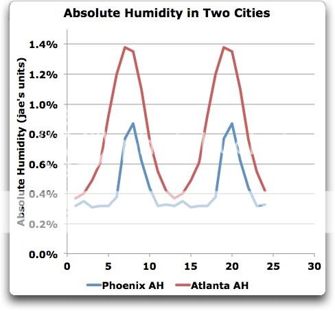
Well, you’ve assumed that the difference between Phoenix and Atlanta is the change from 1% to 3%. I just took a look at the figures for Atlanta. Here they are:
Atlanta Hartsfield Jackson Airport
Month, Specific Humidity (SH), Average Temperature, Absolute Humidity(AH)
Jan, 3.8, 52, 0.37%
Feb, 4.2, 57, 0.40%
Mar, 5.2, 65, 0.49%
Apr, 6.6, 73, 0.61%
May, 10, 80, 0.92%
Jun, 13.3, 86, 1.20%
Jul, 15.4, 89, 1.38%
Aug, 15, 88, 1.35%
Sep, 12.1, 82, 1.10%
Oct, 8.2, 73, 0.76%
Nov, 5.8, 64, 0.55%
Dec, 4.3, 54, 0.42%
As you will notice, the maximum average absolute humidity (AH) in Atlanta in your units is 1.38% …
This is the kind of thing that I expected when I asked for your calculations, jae. Why am I doing your work? You start out by claiming the difference in AH between Phoenix and Atlanta is the difference from 1% (Phoenix) to 3% (Atlanta). But come to find out, you haven’t even bothered to find out the AH in Atlanta, and it’s nothing like 3%, it’s less than half of that …
Since most climate scientists know that, including me, I’m amazed that you think they don’t. See here for a long list of citations to climate scientists saying exactly what you just said.
I’m still waiting for the math regarding your claims. And I still don’t understand your math for the effect of some given increase in water vapor. I mistrust using “simple logic” for that one.
w.
jae, one further comment. I don’t think you can use the density of air at STP as you are doing. The problem is that the absolute humidity (AH) is the density of the water vapor at the instant of measurement. It is defined as mass per cubic metre of air using the conditions (pressure, temperature) occurring at the time of the measurement. It doesn’t use the mass of 1 cubic metre of air at STP.
So if you truly want to use a percentage, to do it properly you have to use the mass of the water as a percentage of the actual mass of the air at prevailing conditions.
In any case, using your method, here’s the results for Atlanta and Phoenix:
You need to think about what difference you would expect this to make, including the effect of the clouds. I hold that the effects of clouds and thunderstorms (few clouds or thunderstorms in Phoenix, lots in Atlanta) will totally swamp the overall warming effect of the difference in water vapor.
All the best,
w.
Jae, you ask:
Well, I guess opinions vary on whether I have answered the question of why Phoenix is hotter than Atlanta despite Atlanta having more GHGs. So let’s settle it by evidence. That’s where I demonstrate that indeed I have answered your question. If I look upthread, I find that I said:
Clearly, I have offered you my explanation for what it is that seems to puzzle you. Your claim that I “HAVE NOT EVEN ATTEMPTED TO ANSWER THAT” is shown by the evidence to be false.
So let me ask you again, which place will be warmer? I say that the effect of having no clouds and no thunderstorms is huge. You’re looking at around 60 W/m2 from the cooling albedo effects of increased clouds alone, and those are dwarfed by the cooling effects of the thunderstorms.
Next, annually the average absolute humidity (AH) in Atlanta (0.79%) is only 80% higher than the annual average AH in Phoenix (0.45%). That’s 1.8-fold, not six-fold as you assert. The difference peaks in May and June, when the AH has risen in Atlanta but not in Phoenix. Those are the only two months where Atlanta has over twice the AH of Phoenix … and the difference is never anywhere near six-fold.
Finally, jae, someone writing in capital letters is taken on the web as shouting. You are shouting about a “SIX-FOLD (AT MINIMUM) INCREASE IN GREENHOUSE GASES IN HUMID AREAS”. The data for the two cities you selected doesn’t show anything like that. Far from six-fold being a minimum, your cities average only a bit less than two-fold … that doesn’t help your credibility.
That’s why I say do the numbers first. It should be you telling me about the true ratio of Atlanta and Phoenix, it’s your line of investigation, not mine. It is an interesting one, to be sure, but at the moment it seems like I’m the one doing it …
w.
Willis:
I guess I’ll have to give up, because you seem to bent on not even trying to understand my point. I am talking about a “doubling” with respect to CO2 EQUIVALENTS, not a doubling of actual amounts of water vapor. The climate scientists are saying that a doubling of CO2 can cause anywhere from 1.2-4 degrees C. But that “doubling” represents a change of ONLY about 0.03 percent of the atmosphere (0.03 now to 0.06 for a doubling). I’m talking about a difference in greenhouse gas that makes the CO2 doubling very minor.
You are right that I shouldn’t use STP for the calculations, due to air density differences. What I really should have done is calculate the volumetric percent so that the mass of the air doesn’t matter. I also used too high a value for abs. humidity in Atlanta, as you show. But the point is still the same. Let me try this again:
7 grams of water/m3 (approx. abs. humidity in Phoenix in July) is 7/18 = 0.39 moles; 0.39 moles water vapor/44.6 moles air/m3 = 0.87% by volume
18 grams water/m3 (approx. abs. humidity in Atlanta in July) is (18/7)(0.87) = 2.23 percent by volume.
So 7 grams of water (abs. humidity of 7 g/m3 or 0.87% by volume) represents 0.87/0.03 = 29 “CO2 equivalents” and 18 grams (abs. humidity of 18 g/m3) = 2.23/0.03 = 74 “CO2 equivalents,” giving a difference of 45 equivalents. So, by this calculation, the increase in GHE in July in Atlanta, relative to Phoenix should be equivalent to increasing the amount of CO2 by 45 times, which would be over 5 “doublings.” And HOH is a much better GHG than CO2, so the true difference would be far greater.
I just would expect to see a much larger GHE in Atlanta, that’s all…Unless the greenhouse effect of water vapor becomes saturated at a fairly low percentage of air volume…
jae, thanks for the post. I think that the problem is that you are dividing the amount of H2O in the atmosphere by the amount of CO2 in the atmosphere to find the relative amounts of “CO2 equivalents”. I see no theoretical justification for the procedure. I don’t see any reason to think that dividing one by the other would give you “CO2 equivalents”.
In any case, I’m not sure what your point is. It is well known that the effect of H20 is an order of magnitude larger than that of CO2. You say “I just would expect to see a much larger GHE in Atlanta, that’s all…”. If GHE ruled the roost, you’d be right. But it doesn’t, there are other stronger factors at play.
You keep ignoring the other effects of water vapor, so I will continue to point them out. If there are thunderstorms and clouds, the peak summertime temperatures don’t go anywhere near as high. This is a difference (clouds and thunderstorms vs clear skies) that is on the order of hundreds of watts per square metre. I have no idea why you’d think that a few watts from the difference in H2O downwelling radiation would be more important than fifty or a hundred watts from having clear skies instead of clouds.
w.
Willis:
Sigh, sigh, sigh, AND SIGH, again! willis, YOU STILL DON’T GET MY POINT!
PLEASE PAY ATTENTION!
You say: “I think that the problem is that you are dividing the amount of H2O in the atmosphere by the amount of CO2 in the atmosphere to find the relative amounts of “CO2 equivalents”. I see no theoretical justification for the procedure. I don’t see any reason to think that dividing one by the other would give you “CO2 equivalents”.
WHAT? READ IT AGAIN, WILLIS! AND AGAIN… I AM NOT SAYING ANYTHING LIKE THAT!
Then you say:
“In any case, I’m not sure what your point is. It is well known that the effect of H20 is an order of magnitude larger than that of CO2. You say “I just would expect to see a much larger GHE in Atlanta, that’s all…”. If GHE ruled the roost, you’d be right. But it doesn’t, there are other stronger factors at play.”
Willis, Willis, Willis, you STILL don’t get my point!!!! You are one of my heros in this hillarious academic bullshit game of “climate science”. BUT LOOK, W., if a change in OCO of 0.03% can affect temperature IN ANY SIGNIFICANT WAY (the “intellegencia says 1-4C or so), then a change in water vapor of many times that should affect temperature much more. To quote you ” It is well known that the effect of H20 is an order of magnitude larger than that of CO2.” WILLIS, IT FOLLOWS THEN THAT YOU SHOULD SEE A BIGGER GREENHOUSE EFFECT IN ATLANTA THAN PHOENIX. BUT I DO NOT SEE IT! I just don’t know how to say it any clearer. I don’t know what else to say..
SHIT, YOU MUST BE A DEMOCRAT!!
jae says:
December 25, 2012 at 7:42 pm
And you must be a fool … Jae, that’s it. I’m through. That’s over the top. I have done what I could to assist you, and you want to talk to me as though I were a child.
Sorry, but you’ve used up all of your second chances with me. I’m done with your nasty insinuations, your innuendoes, and your SHOUTING IN CAPITAL LETTERS. Go away, I’m done here. You can only insult me so many times, then the door slams shut.
It’s too bad, because you had interesting ideas. But YELLING AND SCREAMING doesn’t move me, jae, it just makes you look like a jerkwagon.
So. please go away. Don’t go away mad … just go away. It’s not any fun any more. Your refusal to either explain yourself or pay any attention to anything except your own big mouth has finally reached the level of my gag reflex. I can’t take any more of your childish BS, jae, it’s gotten to the point where it turns my stomach.
It’s over, my friend, over and done. When your name comes up in the future, I’ll just point and laugh. You want to post on my threads? Prepare for not getting any answers from me. You’ve had your fun, acting like you actually were interested in other peoples’ ideas … then refusing to respond when they presented ideas … then yelling and whining like a six-year-old when people refused to respect your lack of details and your absence of facts and your deficiency of explanations … but the game is over.
I’m done with you, my friend. Congratulations, your vote has been officially cancelled by me. Oh, you are free to post here, but I won’t answer, I’ve got better things to do.
Curiously, jae, I do wish you well. I just don’t have time to faff around with your lack of cooperation.
w.
I’ve been following the conversation with one simple-minded thought in mind…the widely reported 33C of average surface temperature increase due to “greenhouse gases”. The simple-minded part is trying to uncover the mysterious mechanics of this average increase. I see the expected modulating mechanisms where peaks (high and low) get constrained, but I don’t see the necessary asymmetry (quick heating and slowed cooling via atmospheric constituents) or exothermic reactions which would do anything to the average. If you add a CO2 molecule that wasn’t otherwise there, surely it’s obvious the cooling rate increases…both via convection and via providing a radiation “portal” when CO2 collides with N2 or O2 molecules.
jae says:
December 24, 2012 at 10:28 am
No, I think you are again misunderstanding what I meaan (and presumably Wilde, also). All I am saying is that the radiation measurement reflects the amount of radiation coming from the GHGs in the atmosphere at the “effective temperature.” Just like you say. The DIFFERENCE is that I think it goes no further than that, and the radiation has no effect on the existing temperature. It is just a property of IR-active molecules in the air. It’s not a “heating mechanism,” or “retardation-of-cooling -mechanism,” no more than “back-conduction” is a heating mechanism in a steel rod stuck in a fire at one end. Otherwise there should be a much bigger difference between wet areas and dry ones, per the above reasoning.
>>>>>>>>>>>>>>>>>>>>>>>>>>>>>>>>>>>>>>>
Except there is a big difference between wet and dry areas.
If you are talking DLR, this paper records actual measurements.
Do not forget the emissivity for water droplets and ice crystals is 0.98.
Some real world data:
For May 2012, Barcelos, Brazil (Lat: 1 South)
Temp: monthly min 20° C
monthly max 33° C
monthly average 26° C
Average humidity 90%
Temperature range was 13° C
For May 2012, Adrar, Algeria (Lat: 27 North)
Temp: monthly min 9° C
monthly max 44° C
, monthly average 30° C
Average humidity around 0%
Temperature range was 35° C
For Tampico, Mexico, (Lat: 22.3° N) – At an Airport on Atlantic ocean
May humidity was avg 70%
min 24.1 ° C
mean 28.8 ° C
max 33.6 ° C
Temperature range was 9.5 ° C
Varied from mostly cloudy to scattered clouds with afternoons clear. 3 days with a bit of drizzle (0.01 to 0.2 inches of rain) one day T-storm
Another city similar in latitude and closer in altitude to Adar Algeria.
Laredo, TX Lat 27.5° N Altitude is 126 m or 413 ft above sea level (Airport)
22.2° C
28.8° C
35.6° C
humidity 62%
Range is 12.4° C
Take a good hard look at those pieces of real world data and ask yourself what it is telling you.
#1. The solar eclipse data tells you the earth & air temperature response (in low humidity) to a change in solar energy is FAST!
#2 The effect of the addition of water vapor (~ 4% globally) is not to raise the temperature but to even the temperature out. The monthly high is ~10C lower and the monthly low is ~10C higher when the GHG H2O is added to the atmosphere in this example. The average temperature is about 4C lower in Brazil despite the fact that Algeria is further north above the tropic of Cancer, For Tampico Mexico and Laredo texas the average is 1C lower that Algeria with the humidity @ur momisugly 60 to 70% (dipping towards the 50% mid day.) It is read at an airport. Some of the difference is from the effect of clouds/albedo but the dramatic effect on the temperature extremes is from the humidity.
I took a rough look at the data from Brazil. Twelve days were sunny. I had to toss the data for two days because it was bogus. (see link) The average humidity was 80% for those ten days. The high was 32 with a range of 1.7C and the low was 22.7C with a range of 2.8C. Given the small range in values over the month the data is probably a pretty good estimate for the effects of humidity only. You still get the day-night variation of ~ 10C with a high humidity vs a day-night variation of 35C with very low humidity and the average temp is STILL going to be lower when the humidity is high.
ALTITUDE:
Tampico Mexico ~ Elevation: 15 metres (49 feet)
Barcelos, Brazil elevation ~ 30 meters (100 ft)
Adrar, Algeria ~ Elevation: 280 metres (920 feet) a drop in temperature of ~ 4C due to altitude: http://www.engineeringtoolbox.com/air-altitude-temperature-d_461.html
One would expect a drop in temperature of ~ 4C due to altitude for Adrar, Algeria.
This data would indicate GHGs have two effects. One is to even out the temperature and the second is to act as a “coolant” at least if the GHG is H2O.
The latent heat of evaporation could be why the average is 4C lower when in Brazil vs Algeria. As one of the commenters here at WUWT mentioned using temperature without humidity to estimate the global heat content is bad physics.
Data Brazil:
http://classic.wunderground.com/history/station/82113/2012/5/22/MonthlyHistory.html
http://www.climate-charts.com/Locations/b/BZ82113.php
Map: http://www.worldatlas.com/webimage/countrys/samerica/brsa.gif
Data Algeria:
http://www.wunderground.com/history/airport/DAUA/2012/5/20/MonthlyHistory.html
http://www.climate-charts.com/Locations/a/AL60620.php
Map: http://www.worldatlas.com/webimage/countrys/africa/dzafrica.gif
Data for Mexico:
http://classic.wunderground.com/history/airport/MMTM/2012/5/19/DailyHistory.html
http://www.tampico.climatemps.com/
http://www.zonu.com/fullsize1-en/2009-09-17-5311/Satellite-image-of-Tampico.html
Photos Adrar, Algeria and Barcelos, Brazil
http://algeriaspace.blogspot.com/2007/07/photos-satellite-ville-adrar-algerie.html
http://www.maplandia.com/brazil/airports/barcelos-airport/
kencoffman (@kencoffman) says:
December 26, 2012 at 6:11 am
Ken, for the mechanisms see my two posts, The Steel Greenhouse and People Living in Glass Planets.
All the best,
w.
Gail Combs says:
December 26, 2012 at 6:21 am
Thanks, Gail. What the real world data tell me is that it is naive to try to tease out a heating signal from water vapor by just grabbing a bunch of cities and looking at their temperatures.
The part that you and jae keep sailing right on past is that you have to, you must, you need to, you are required to account for the confounding variables. You can’t just say, as jae does, that Phoenix is warmer than Atlanta despite having less water, so that proves the water vapor doesn’t heat anything. That’s grade school understanding of attribution.
The confounding variables that you need to account for include variables unrelated to water, such as altitude or soil type or distance from the ocean, along with much more difficult confounding variables such as clouds and thunderstorms and evaporative cooling and ground cover that are a function of water itself. These latter ones are harder to account for, since they vary in proportion with water vapor.
So no, you cannot just grab a handful of cities in Brazil, Mexico, and Algeria, look at the temperatures and the relative humidity, and declare the game over.
I have shown above one way that actually works that shows the difference in the DLR, which I described above. This was to calculate how high the effective radiative level was above the ground (or alternately how cool the radiative level was) in moist and dry areas. This calculation shows that the water vapor indeed does increase the DLR …
But of course, to you and jae this finding is anathema, so you just ignore it.
Another way to reduce, if not get rid of, the confounding variables is to look at different times in the same location. Look at the data for Goodwin Creek, for example, month by month. See if the DLR varies in phase with the water vapor.
But please, Gail, please, don’t do what jae does and claim that he has discovered some new kind of DLR radiation that doesn’t contain energy. DLR contains energy, we’ve measured it many many times. We know just how much energy the DLR contains, and we know that energy can’t be created or destroyed … which means that when DLR is absorbed an object, that object ends up warmer than it would be in the absence of DLR. In other words, jae’s claim that DLR that contains no energy is just his desperate attempt to salvage his incorrect understanding.
w.
Willis:
So you can comment to Gail and disparage me and my thoughts on your tirade, and I cannot argue back? You are, indeed a Democrat! Pure Obama-style-authoritarian, fella….
Do you have ANY concept of fairness??
But I’m relieved, in a way, that I am now an outcast here, because, SIR, you are NOT a listener, but some kind of big-headed “boss.” YOU STILL DON’T GET MY POINT, AFTER ALL THIS TALK. Gail doesn’t either.
And using CAPS is nowhere near as nasty, angry, hot-headed as your post was. Hypocrite!
I’m again weary of this conversation, and I give up here, AGAIN!
Good bye.
jae says:
December 26, 2012 at 6:02 pm
I don’t have the power to stop you from arguing back, jae, or to stop you from arguing front for that matter. Nor would I stop you if I could. Nor did I say that you couldn’t argue back.
So you are arguing against something that, as far as I know, I never said.
Next time, quote what I said so we can all be clear about just what is the latest thing that you are upset with me about. It changes so often, I can’t keep track.
Of course, you include the requisite number of insults …
I’m sure it’s Gail’s fault for not understanding your brilliance, jae. I’ll speak sharply to her and tell her to shape up …
w.
Kencoffman says…
“If you add a CO2 molecule that wasn’t otherwise there, surely it’s obvious the cooling rate increases”……….. Yes Ken, you’re right , gases don’t add energy, but disperse it. All gases dissipate heat.