Some people cite scientists saying there is a “CO2 control knob” for Earth. No doubt there is, but due to the logarithmic effect of CO2, I think of it like a fine tuning knob, not the main station tuner. That said, a new data picture is emerging of an even bigger knob and lever; a nice bright yellow one.

A few months back, I found a website from NOAA that provides an algorithm and downloadable program for spotting regime shifts in time series data. It was designed by Sergei Rodionov of the NOAA Bering Climate and Ecosystem Center for the purpose of detecting shifts in the Pacific Decadal Oscillation.
Regime shifts are defined as rapid reorganizations of ecosystems from one relatively stable state to another. In the marine environment, regimes may last for several decades and shifts often appear to be associated with changes in the climate system. In the North Pacific, climate regimes are typically described using the concept of Pacific Decadal Oscillation. Regime shifts were also found in many other variables as demonstrated in the Data section of this website (select a variable and then click “Recent trends”).
But data is data, and the program doesn’t care if it is ecosystem data, temperature data, population data, or solar data. It just looks for and identifies abrupt changes that stabilize at a new level. For example, a useful application of the program is to look for shifts in weather data, such as that caused by the PDO. Here we can clearly see the great Pacific Climate Shift of 1976/77:
Another useful application is to use it to identify station moves that result in a temperature shift. It might also be applied to proxy data, such as ice core Oxygen 18 isotope data.
But the program was developed around the PDO. What drives the PDO? Many say the sun, though there are other factors too. It follows to reason then the we might be able to look for solar regime shifts in PDO driven temperature data.
Alan of AppInSys found the same application and has done just that, and the results are quite interesting. The correlation is well aligned, and it demonstrates the solar to PDO connection quite well. I’ll let him tell his story of discovery below. – Anthony
=================================
Climate Regime Shifts
The notion that climate variations often occur in the form of ‘‘regimes’’ began to become appreciated in the 1990s. This paradigm was inspired in large part by the rapid change of the North Pacific climate around 1977 [e.g., Kerr, 1992] and the identification of other abrupt shifts in association with the Pacific Decadal Oscillation (PDO) [Mantua et al., 1997].” [http://www.beringclimate.noaa.gov/regimes/Regime_shift_algorithm.pdf]
Pacific Regime Shifts
Hare and Mantua, 2000 (“Empirical evidence for North Pacific regime shifts in 1977 and 1989”): “It is now widely accepted that a climatic regime shift transpired in the North Pacific Ocean in the winter of 1976–77. This regime shift has had far reaching consequences for the large marine ecosystems of the North Pacific. Despite the strength and scope of the changes initiated by the shift, it was 10–15 years before it was fully recognized. Subsequent research has suggested that this event was not unique in the historical record but merely the latest in a succession of climatic regime shifts. In this study, we assembled 100 environmental time series, 31 climatic and 69 biological, to determine if there is evidence for common regime signals in the 1965–1997 period of record. Our analysis reproduces previously documented features of the 1977 regime shift, and identifies a further shift in 1989 in some components of the North Pacific ecosystem. The 1989 changes were neither as pervasive as the 1977 changes nor did they signal a simple return to pre-1977 conditions.”
[http://www.sciencedirect.com/science?_ob=ArticleURL&_udi=B6V7B-41FTS3S-2…]
Overland et al “North Pacific regime shifts: Definitions, issues and recent transitions”
[http://www.pmel.noaa.gov/foci/publications/2008/overN667.pdf]: “climate variables for the North Pacific display shifts near 1977, 1989 and 1998.”
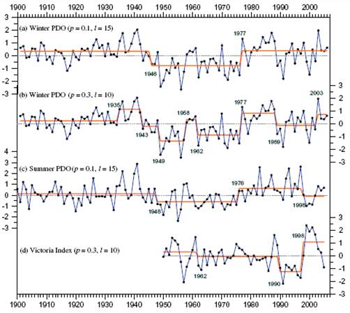
The following figure from the above paper show analysis of PDO and Victoria Index using the Rodionov regime detection algorithm. A regime shift is also detected around 1947-48.
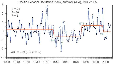
The following figure shows regime shift detection for the summer PDO, showing shifts at 1948, 1976 and 1998.
[http://www.beringclimate.noaa.gov/data/Images/PDOs_FigRegime.html]
(For detailed information on the 1976/77 climate shift,
see: http://www.appinsys.com/GlobalWarming/The1976-78ClimateShift.htm)
Regime Shift Detection in Annual Temperature Anomaly Data
The NOAA Bering Climate web site provides the algorithm for regime shift detection developed by Sergei Rodionov [http://www.beringclimate.noaa.gov/regimes/index.html]. The following analyses use the Excel VBA regime change algorithm version 3.2 from this web site.
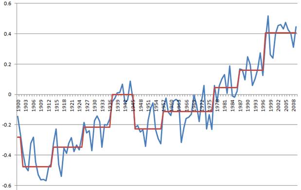
The following figure shows the regime analysis of the HadCRUT3 annual global annual average temperature anomaly data from the Met Office Hadley Centre for 1895 to 2009 [http://hadobs.metoffice.com/hadcrut3/diagnostics/global/nh+sh/annual].
The analysis was run based on the mean using a significance level of 0.1, cut-off length of 10 and Huber weight parameter of 2 using red noise IP4 subsample size 6. Regime changes are identified in 1902, 1914, 1926, 1937, 1946, 1957, 1977, 1987, and 1997. Running the analysis based on the variance rather than the mean results in regime changes in the bold years listed above.
Regime Shift Relationship to Solar Cycle
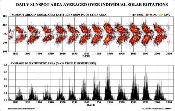
The NASA Solar Physics web site provides the following figure showing sunspot area.
[http://solarscience.msfc.nasa.gov/SunspotCycle.shtml]
The following figure compares the Hadley (HadCrut3) monthly global average temperature (from [http://hadobs.metoffice.com/hadcrut3/diagnostics/global/nh+sh/]) overlaid with the regime change line (red line) shown previously, along with the sunspot area since 1900. The sunspot cycle is approximately 11 years. The sun’s magnetic field reverses with each sunspot cycle and thus after two sunspot cycles the magnetic field has completed a cycle – a Hale Cycle – and is back to where it started. Thus a complete magnetic sunspot cycle is approximately 22 years. The figure marks the onset of odd-numbered cycles with a vertical red line, even-numbered cycles with a green line.
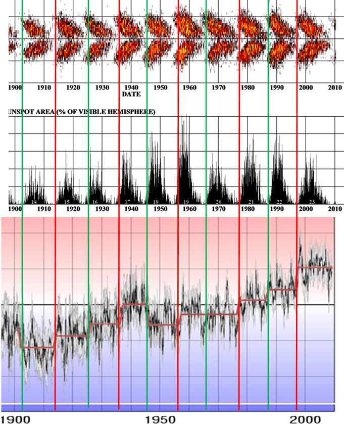
From the figure above it can be seen that the regime changes correspond to the onset of solar cycles and occur when the “butterfly” is at its widest. The most significant warming regime shifts occur at the start of odd-numbered cycles (1937, 1957, 1977, 1997). Each odd-numbered cycle (red lines above) has resulted in a temperature-increase regime shift. Even-numbered cycles (green lines above) have been inconsistent, with some resulting in temperature-decrease regime shifts (1902, 1946) or minor temperature-increase shifts (1926, 1987).
An unusual one is the 1957 – 1966 cycle, which in the monthly data shown above visually looks like a temperature-increase shift in 1957 followed by a temperature-decrease shift in 1964 but the regime detection algorithm did not identify it. This is likely due to the use of annually averaged data in the regime detection algorithm.
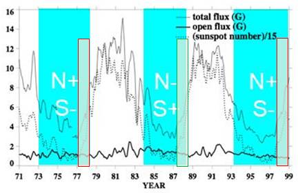
The following figure shows the relative polarity of the Sun’s magnetic poles for recent sunspot cycles along with the solar magnetic flux [www.bu.edu/csp/nas/IHY_MagField.ppt]. The regime change periods are highlighted by the red and green boxes. Each one occurs on as the solar cycle is accelerating. The onset of an odd-numbered sunspot cycle (1977-78, 1997-98) results in the relative alignment of the Earth’s and the Sun’s magnetic fields (positive North pole on the Sun) allowing greater penetration of the geomagnetic storms into the Earth’s atmosphere. “Twenty times more solar particles cross the Earth’s leaky magnetic shield when the sun’s magnetic field is aligned with that of the Earth compared to when the two magnetic fields are oppositely directed” [http://www.nasa.gov/mission_pages/themis/news/themis_leaky_shield.html]
The following figure shows the longitudinally averaged solar magnetic field. This “magnetic butterfly diagram” shows that the sunspots are involved with transporting the field in its reversal. The Earth’s temperature regime shifts are indicated with the superimposed boxes – red on odd numbered solar cycles, green on even.
[http://solarphysics.livingreviews.org/open?pubNo=lrsp-2010-1&page=articlesu8.html]
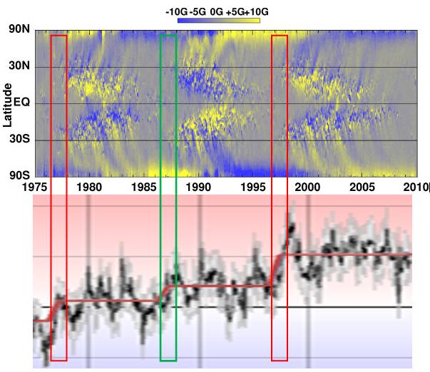
The Earth’s temperature regime shift occurs as the solar magnetic field begins its reversal.
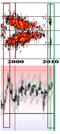
Solar Cycle 24
Solar cycle 24 is in its initial stage after getting off to a late start. An El Nino occurred in the first part of 2010. This may be the start of the next regime shift.
Climate Regime Shifts
[last update: 2010/07/04]
|
“The notion that climate variations often occur in the form of ‘‘regimes’’ began to become appreciated in the 1990s. This paradigm was inspired in large part by the rapid change of the North Pacific climate around 1977 [e.g., Kerr, 1992] and the identification of other abrupt shifts in association with the Pacific Decadal Oscillation (PDO) [Mantua et al., 1997].” [http://www.beringclimate.noaa.gov/regimes/Regime_shift_algorithm.pdf]
|
|
Pacific Regime Shifts
Hare and Mantua, 2000 (“Empirical evidence for North Pacific regime shifts in 1977 and 1989”): “It is now widely accepted that a climatic regime shift transpired in the North Pacific Ocean in the winter of 1976–77. This regime shift has had far reaching consequences for the large marine ecosystems of the North Pacific. Despite the strength and scope of the changes initiated by the shift, it was 10–15 years before it was fully recognized. Subsequent research has suggested that this event was not unique in the historical record but merely the latest in a succession of climatic regime shifts. In this study, we assembled 100 environmental time series, 31 climatic and 69 biological, to determine if there is evidence for common regime signals in the 1965–1997 period of record. Our analysis reproduces previously documented features of the 1977 regime shift, and identifies a further shift in 1989 in some components of the North Pacific ecosystem. The 1989 changes were neither as pervasive as the 1977 changes nor did they signal a simple return to pre-1977 conditions.” [http://www.sciencedirect.com/science?_ob=ArticleURL&_udi=B6V7B-41FTS3S-2…]
Overland et al “North Pacific regime shifts: Definitions, issues and recent transitions” [http://www.pmel.noaa.gov/foci/publications/2008/overN667.pdf]: “climate variables for the North Pacific display shifts near 1977, 1989 and 1998.”
The following figure from the above paper show analysis of PDO and Victoria Index using the Rodionov regime detection algorithm. A regime shift is also detected around 1947-48.
The following figure shows regime shift detection for the summer PDO, showing shifts at 1948, 1976 and 1998. [http://www.beringclimate.noaa.gov/data/Images/PDOs_FigRegime.html]
(For detailed information on the 1976/77 climate shift, see: http://www.appinsys.com/GlobalWarming/The1976-78ClimateShift.htm)
|
|
Regime Shift Detection in Annual Temperature Anomaly Data
The NOAA Bering Climate web site provides the algorithm for regime shift detection developed by Sergei Rodionov [http://www.beringclimate.noaa.gov/regimes/index.html]. The following analyses use the Excel VBA regime change algorithm version 3.2 from this web site.
The following figure shows the regime analysis of the HadCRUT3 annual global annual average temperature anomaly data from the Met Office Hadley Centre for 1895 to 2009 [http://hadobs.metoffice.com/hadcrut3/diagnostics/global/nh+sh/annual].
The analysis was run based on the mean using a significance level of 0.1, cut-off length of 10 and Huber weight parameter of 2 using red noise IP4 subsample size 6. Regime changes are identified in 1902, 1914, 1926, 1937, 1946, 1957, 1977, 1987, and 1997. Running the analysis based on the variance rather than the mean results in regime changes in the bold years listed above.
|
|
Regime Shift Relationship to Solar Cycle
The NASA Solar Physics web site provides the following figure showing sunspot area. [http://solarscience.msfc.nasa.gov/SunspotCycle.shtml]
The following figure compares the Hadley (HadCrut3) monthly global average temperature (from [http://hadobs.metoffice.com/hadcrut3/diagnostics/global/nh+sh/]) overlaid with the regime change line (red line) shown previously, along with the sunspot area since 1900. The sunspot cycle is approximately 11 years. The sun’s magnetic field reverses with each sunspot cycle and thus after two sunspot cycles the magnetic field has completed a cycle – a Hale Cycle – and is back to where it started. Thus a complete magnetic sunspot cycle is approximately 22 years. The figure marks the onset of odd-numbered cycles with a vertical red line, even-numbered cycles with a green line.
From the figure above it can be seen that the regime changes correspond to the onset of solar cycles and occur when the “butterfly” is at its widest. The most significant warming regime shifts occur at the start of odd-numbered cycles (1937, 1957, 1977, 1997). Each odd-numbered cycle (red lines above) has resulted in a temperature-increase regime shift. Even-numbered cycles (green lines above) have been inconsistent, with some resulting in temperature-decrease regime shifts (1902, 1946) or minor temperature-increase shifts (1926, 1987).
An unusual one is the 1957 – 1966 cycle, which in the monthly data shown above visually looks like a temperature-increase shift in 1957 followed by a temperature-decrease shift in 1964 but the regime detection algorithm did not identify it. This is likely due to the use of annually averaged data in the regime detection algorithm.
The following figure shows the relative polarity of the Sun’s magnetic poles for recent sunspot cycles along with the solar magnetic flux [www.bu.edu/csp/nas/IHY_MagField.ppt]. The regime change periods are highlighted by the red and green boxes. Each one occurs on as the solar cycle is accelerating. The onset of an odd-numbered sunspot cycle (1977-78, 1997-98) results in the relative alignment of the Earth’s and the Sun’s magnetic fields (positive North pole on the Sun) allowing greater penetration of the geomagnetic storms into the Earth’s atmosphere. “Twenty times more solar particles cross the Earth’s leaky magnetic shield when the sun’s magnetic field is aligned with that of the Earth compared to when the two magnetic fields are oppositely directed” [http://www.nasa.gov/mission_pages/themis/news/themis_leaky_shield.html]
The following figure shows the longitudinally averaged solar magnetic field. This “magnetic butterfly diagram” shows that the sunspots are involved with transporting the field in its reversal. The Earth’s temperature regime shifts are indicated with the superimposed boxes – red on odd numbered solar cycles, green on even. [http://solarphysics.livingreviews.org/open?pubNo=lrsp-2010-1&page=articlesu8.html]
The Earth’s temperature regime shift occurs as the solar magnetic field begins its reversal.
|
|
Solar Cycle 24
Solar cycle 24 is in its initial stage after getting off to a late start. An El Nino occurred in the first part of 2010. This may be the start of the next regime shift.
|
@tallbloke says:
July 12, 2010 at 1:56 pm
“I wish I understood why Leif and so many of his colleagues are so resistant to the study of waves and cycles.”
1) astrology is the biggest heresy.
2) they cannot find them in the data !
Ulric Lyons says:
July 12, 2010 at 2:13 pm
either way, it is the last BIG spike in the graph:
http://www.leif.org/research/FFT%20of%20IMF%20Direction.png
Those spikes out there are not statistically significantly different. All they show is that there is power around the solar cycle.
Ulric Lyons says:
July 12, 2010 at 2:23 pm
2) they cannot find them in the data !
You cannot gather roses where no roses grow…
maksimovich says:
July 10, 2010 at 5:08 pm
Bob Tisdale says:
July 10, 2010 at 1:07 pm
Stephen Wilde: My question, “Based on your observations, how many degrees latitude are the variations in polar cycles (AO & SAM) pushing the clouds equatorward in response to decreasing solar activity?”
Ill posed problems,ie multiple time series.
Firstly would it not be more correct to examine when say radiative forcing ( insolation ) is greatest, which would be the inter annual solar cycle.Here the annual excursions of the extratropical storm tracks with their latitudinal effects are well described in the literature eg Ramanathan
The enormous cooling effect of extratropical storm track cloud systems
Extra-tropical storm track cloud systems provide about 60% of the total cooling effect of clouds [2]. The annual mean forcing from these cloud systems is in the range of –45 to –55 W m–2 and effectively these cloud systems are shielding both the northern and
the southern polar regions from intense radiative heating. Their spatial extent towards the tropics moves with the jet stream, extending farthest towards the tropics
(about 35 deg latitude) during winter and retreating polewards (polewards of 50 deg
latitude) during summer. This phenomenon raises an important question related to past climate dynamics. During the ice age, due to the large polar cooling, the northern hemisphere jet stream extended more southwards. But have the extra tropical cloud systems also moved southward? The increase in the negative forcing would have exerted a major positive feedback on the ice age cooling. There is a curious puzzle about the existence of these cooling clouds. The basic function of the extra tropical dynamics is to export heat polewards.
While the baroclinic systems are efficient in transporting heat, the enormous negative
radiative forcing (Fig. 2) associated with these cloud systems seems to undo the
poleward transport of heat by the dynamics. The radiative effect of these systems is working against the dynamical effect. Evidently,we need better understanding of the dynamic-thermodynamic coupling between these enormous cooling clouds and the
equator-pole temperature gradient, and greenhouse forcing.
__________________________________Reply;
All of this and nobody looks at the Lunar declinational tides in the atmosphere?
I think you will find a much better signal in the patterns of jet stream positions and lunar declination periods.
The composite is built around the Lunar declinational variation and the Earth’s Heliocentric conjunctions with the other planets, modulated together with the solar output, to form the driving forces of all of the periodic features of the recognized global circulation patterns.
Data found soon to be processed, just need high speed connection to the internet, and a little software yet.
tallbloke says:
July 12, 2010 at 12:18 pm
physicists with fine abilities such as yours to come up with the details of the viable mechanism I’ve intuited.
Scientific debate is not about intuition, leaving it to others to explain it, it is about winning the argument on its own scientific merit. Your above comment gives the set and match to Leif.
Leif Svalgaard says:
July 12, 2010 at 12:19 pm
“OK, Einstein, we are awaiting your correct analysis.”
I thought a stein was a mug! I`ll trawl through;
http://www.ngdc.noaa.gov/stp/solar/corona.html
and see what is apparent, shame it does not do the early 1930`s, our distant decendants will be spoilt for data !
Ulric Lyons says:
July 12, 2010 at 3:12 pm
and see what is apparent, shame it does not do the early 1930`s, our distant decendants will be spoilt for data !
We didn’t know about coronal holes [in the modern meaning] before ~1970.
Pamela Gray says:
July 12, 2010 at 3:09 pm (Edit)
Scientific debate is not about intuition, leaving it to others to explain it, it is about winning the argument on its own scientific merit. Your above comment gives the set and match to Leif.
You’re late. Anyway, I’m not playing tennis. And I’m not arguing or debating, I’m just stating it as it is. We’ll use our brains to discover the relationships, then they’ll rustle up some whizzo technology to confirm it.
It was ever thus. Look what happened to poor bloody Tesla. A man strong on intuition and short on business acumen.
@Leif Svalgaard says:
July 12, 2010 at 3:16 pm
http://www.ngdc.noaa.gov/stp/solar/corona.html
I just glanced at it earlier and saw `1939`, yes the hole records start 1970, and no solar wind speed is given so that`s no use to me then.
Yes, thats what I need too. A good record of solar wind speed. From the space age only if it’s accurate, directly measured rather than inferred, and up to date.
tallbloke says:
July 12, 2010 at 11:01 pm
Yes, thats what I need too. A good record of solar wind speed. From the space age only if it’s accurate, directly measured rather than inferred, and up to date.
http://omniweb.gsfc.nasa.gov/form/dx1.html
Many thanks Leif, useful. Is there any longer term graph or downloadable data I can refer to for context which is accurate in your view? If so what is the proxy?
Just come across an interesting paper about the ‘extended’ solar cycle which details some anomalous SC24 behaviour as compared with the two previous cycles…
The Progress of Solar Cycle 24 at High Latitudes
Authors: Richard C. Altrock (Air Force Research Laboratory, NSO/SP, Sunspot, NM, USA) – Submitted on 11 Feb 2010
Abstract: The “extended” solar cycle 24 began in 1999 near 70 degrees latitude, similarly to cycle 23 in 1989 and cycle 22 in 1979. The extended cycle is manifested by persistent Fe XIV coronal emission appearing near 70 degrees latitude and slowly migrating towards the equator, merging with the latitudes of sunspots and active regions (the “butterfly diagram”) after several years. Cycle 24 began its migration at a rate 40% slower than the previous two solar cycles, thus indicating the possibility of a peculiar cycle. However, the onset of the “Rush to the Poles” of polar crown prominences and their associated coronal emission, which has been a precursor to solar maximum in recent cycles (cf. Altrock 2003), has just been identified in the northern hemisphere. Peculiarly, this “Rush” is leisurely, at only 50% of the rate in the previous two cycles. The properties of the current “Rush to the Poles” yields an estimate of 2013 or 2014 for solar maximum.
Full paper is available free here:-
http://arxiv.org/pdf/1002.2401v1
tallbloke says:
July 13, 2010 at 12:51 am
Many thanks Leif, useful. Is there any longer term graph or downloadable data I can refer to for context which is accurate in your view? If so what is the proxy?
Well, you did say that you wanted direct spacecraft data, not inferred data [from proxies?]. There is also a time resolution issue. The spacecraft data has good time resolution [hour to seconds], proxies will be months to a year. What do you really want ?
Tenuc says:
July 13, 2010 at 1:01 am
Just come across an interesting paper about the ‘extended’ solar cycle which details some anomalous SC24 behaviour as compared with the two previous cycles…
There is very likely is no ‘extended’ cycle, as the activity interpreted as part of the extended cycle seems to be just remnants of the current cycle, rather than stuff from the next cycle: http://www.leif.org/EOS/ApJ_716_1_693.pdf
This subject is controversial at this time.
tallbloke says:
July 12, 2010 at 11:01 pm
Yes, thats what I need too. A good record of solar wind speed. From the space age only if it’s accurate, directly measured rather than inferred, and up to date.
http://omniweb.gsfc.nasa.gov/form/dx1.html
___________________________________________________
This site is the bees knees for studying every plasma and magnetic parameter in relation to short term surface temperature change.
With my Planetary Ordered Solar Theory, I can predict weekly or less temperature changes highly accurately a great distance ahead, and hindcast at this definition back through centuries, so I know what is doing it, the only missing piece of the puzzle is the exact mechanisms. Solar wind velocity shows a very good correlation to short term changes, but other parameters need to be checked too. Then we need to discover the nature of the short term heat increases, are we dealing with higher IR levels with higher solar wind speed/density/pressure, as well as short bursts of surface warming from higher UV when sunspot regions are more active?
When the solar cycle is seen from a solar wind point of view, we can get a better picture of the nature of temperature events at different parts of the solar cycle, such that solar wind can be very turbulent around solar max, but less constant, giving typically, the greater short term extremes in temperatures around max, from heat waves, to the higher occurence of cold winters at solar max. It is all down to timing of these short term changes as to which hemisphere gets the cold winter, if at all. A quick scan though any long monthly temperature series at the coldest winters in the last 2-3 hudred years reveals +ve temperature anomalies usually within 2-4 months of the very coldest months. P.O.S.T. can demonstate why.
Leif Svalgaard says:
July 13, 2010 at 1:05 am (Edit)
Well, you did say that you wanted direct spacecraft data, not inferred data [from proxies?]. There is also a time resolution issue. The spacecraft data has good time resolution [hour to seconds], proxies will be months to a year. What do you really want ?
I want it all, I want it now! (Tm Freddie Mercury)
Seriously, I’m very grateful and happy with the accurate satellite data, because I can use that for a case study in the short term. It would be useful also to have a proxy reconstruction of solar wind speed going back as far as possible towards the beginning of the sunspot record, if such a thing exists.
Do you know if the magnetic flux lines involved in reconnection events between the Sun and Earth (or Sun and any other planets) get curved by the solar wind variation? I understand what you say about solar wind going in straight lines out from the sun, but if there is a big coronal hole emanating faster solar wind from a solar region, this will leave a spiral trace in the IMF as the sun turns. I’m wondering if this will affect the flux lines or magnetic ‘ropes’ forming between the Sun and the magnetospheres of planets.
Thanks
@richard Holle says:
July 12, 2010 at 2:51 pm
Richard, if I may ask you a question, as a long range forecaster, I am highly interested in Lunar effects on weather events and types, I have looked at USA tornado events in respect to Lunar declination, and could not find anything conclusive, do you have a tabulated list of these?
With the sea tides, spring tides occur just after every full and new moon, with the highest at the full moons around the vernal equinox, and the new moons around the autumn equinox. Obviously highs and lows of delination around the solstices will be at full and new moon, but at the equinoxes, extremes of declination occur at the quarter moons, one low, and one high, and there is very little difference in tide hight between them, how does this declination issue make a difference to atmospheric circulation, but not to the sea tides?
tallbloke says:
July 13, 2010 at 5:00 am
It would be useful also to have a proxy reconstruction of solar wind speed going back as far as possible towards the beginning of the sunspot record, if such a thing exists.
Geomagnetic activity A depends on the solar wind speed V and the magnetic field strength B [and a few other things to second order. Generally A ~ B*V^2. Now, A is known with three-hours resolution back to the 1840s. On that short time scale, we do not [yet] know how the separate B and V. On time scales of a month to a year, we [I, actually] have figured out how to separate B and V and can reconstruct both. Here is how: http://www.leif.org/research/IAGA2008LS-final.pdf
if there is a big coronal hole emanating faster solar wind from a solar region, this will leave a spiral trace in the IMF as the sun turns. I’m wondering if this will affect the flux lines or magnetic ‘ropes’ forming between the Sun and the magnetospheres of planets.
The filed lines are always curved into a spiral. For high solar wind speed the spiral is less strongly would, and for low speed the spiral is more tightly wound. At the outer planets, the spiral is wound around the Sun several times. The notion of ropes ‘forming’ between the Sun and the planets, is misguided. The ropes or field lines are there all the time, planets or no planets. The solar wind [ropes and all] sweeps past the planets at supersonic speed [11 times as fast as the magnetic field can propagate], in the process reconnecting with the planets magnetic field [about half the time, depending on the angle between the two fields – which varies randomly from hour to hour] and dragging the planetary field with it downstream for a short while [three hours for the Earth, a day for the larger planets]. Eventually the dragging comes to an end [think stretching a rubber band until it snaps] and the connection is broken. The solar wind and the Sun have no knowledge of the planet before hitting it [because moving faster than Alfven waves can propagate], just like you cannot hear a supersonic jet aircraft [or bullet] approaching you.
The effect of the solar wind speed on this process is to increase the number of field lines brought up to the planet: faster speed, more field lines per unit time, just like the speed of a flowing river determines how much water is flowing. But this, again, has no influence on anything upstream. If anything, the faster the wind, the more supersonic it gets and the less is any influence.
Leif Svalgaard says:
July 13, 2010 at 1:37 am
“(Tenuc says:
July 13, 2010 at 1:01 am
Just come across an interesting paper about the ‘extended’ solar cycle which details some anomalous SC24 behaviour as compared with the two previous cycles…)
There is very likely is no ‘extended’ cycle, as the activity interpreted as part of the extended cycle seems to be just remnants of the current cycle, rather than stuff from the next cycle: http://www.leif.org/EOS/ApJ_716_1_693.pdf
This subject is controversial at this time.”
Thanks for the above link, Leif, another interesting paper. Surprisingly some of the diagrams of the Coronal field-line configurations modelled in Fig 8 are very similar to those produced by a Tesla coil when over-driven and the primary and secondary coils are out of phase.
If, as you say, the Run to the Poles is a remnant of the current cycle, does this mean that the weaker than normal poloidal field is direct result of the weaker than normal toroidal field, or are cause and effect the other way round?
Leif, very helpful, thanks again. Time to revisit the solar physics 101 page you linked for me somewhere ^upthere and do some sums and sketches.
Tenuc says:
July 13, 2010 at 7:42 am
very similar to those produced by a Tesla coil when over-driven and the primary and secondary coils are out of phase.
The Sun has some of that as the toroidal and poloidal fields are out off phase. One should not take the similarity too far, though. There is no big single coil driving everything, but millions of little ones interacting and producing the sun’s magnetic field as an ’emergent’ property.
If, as you say, the Run to the Poles is a remnant of the current cycle, does this mean that the weaker than normal poloidal field is direct result of the weaker than normal toroidal field, or are cause and effect the other way round?
Both ! If there is less toroidal filed you get less polar fields, and with less polar fields , the next cycle will have less toroidal field. Taken literally, this would mean that cycles would get ever smaller [or bigger for the case of more field]. However, there is enough randomness in the system that such a streak of ever-smaller [or bigger] cycles is quickly broken. The poloidal field is only 1/1000 of the toroidal field and corresponds to the field from only a handful of sunspots, compared to the thousands generated in each cycle.
Tenuc says:
July 13, 2010 at 7:42 am
If, as you say, the Run to the Poles is a remnant of the current cycle…
More precisely, the Rush occurs during the first third or so of a given cycle. There is a filament [bright green corona] separating the old polar fields [from the minimum] and the new flux [with opposite polarity] moving towards the pole. You can see this filament as the dark horizontal line crossing the disk near the north pole here:
http://sdowww.lmsal.com/sdomedia/SunInTime/2010/07/13/l_211_193_171.jpg
To see the magnetic field: http://sdowww.lmsal.com/sdomedia/SunInTime/2010/07/13/f_HMImag_171.jpg
Then click on the image to make it larger.
The magnetic field is the small orange [polarity into the Sun] and blue [out of the Sun] specks covering the surface. Note the preponderance of blue specks near the north pole above [at higher latitude] the filament and the orange specs below the filament. The orange field slowly eats away the blue as the cycle moves towards maximum, and the dividing line moves polewards [rush to the poles] until all the blue is gone, replaced by orange.
Thanks for the explanation, Leif, I’ve often wondered how the the two fields relate.
Presumably the same thing will happen in the southern hemisphere as SC24 develops and we approach the cycle maximum, whatever that may bring.
BTW, the SDO images are amazing, link now bookmarked, thanks.