Some people cite scientists saying there is a “CO2 control knob” for Earth. No doubt there is, but due to the logarithmic effect of CO2, I think of it like a fine tuning knob, not the main station tuner. That said, a new data picture is emerging of an even bigger knob and lever; a nice bright yellow one.

A few months back, I found a website from NOAA that provides an algorithm and downloadable program for spotting regime shifts in time series data. It was designed by Sergei Rodionov of the NOAA Bering Climate and Ecosystem Center for the purpose of detecting shifts in the Pacific Decadal Oscillation.
Regime shifts are defined as rapid reorganizations of ecosystems from one relatively stable state to another. In the marine environment, regimes may last for several decades and shifts often appear to be associated with changes in the climate system. In the North Pacific, climate regimes are typically described using the concept of Pacific Decadal Oscillation. Regime shifts were also found in many other variables as demonstrated in the Data section of this website (select a variable and then click “Recent trends”).
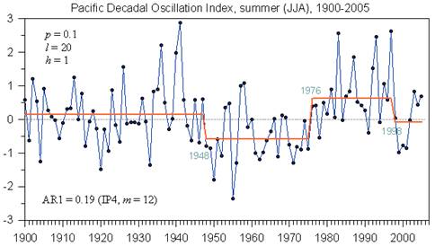
But data is data, and the program doesn’t care if it is ecosystem data, temperature data, population data, or solar data. It just looks for and identifies abrupt changes that stabilize at a new level. For example, a useful application of the program is to look for shifts in weather data, such as that caused by the PDO. Here we can clearly see the great Pacific Climate Shift of 1976/77:
Another useful application is to use it to identify station moves that result in a temperature shift. It might also be applied to proxy data, such as ice core Oxygen 18 isotope data.
But the program was developed around the PDO. What drives the PDO? Many say the sun, though there are other factors too. It follows to reason then the we might be able to look for solar regime shifts in PDO driven temperature data.
Alan of AppInSys found the same application and has done just that, and the results are quite interesting. The correlation is well aligned, and it demonstrates the solar to PDO connection quite well. I’ll let him tell his story of discovery below. – Anthony
=================================
Climate Regime Shifts
The notion that climate variations often occur in the form of ‘‘regimes’’ began to become appreciated in the 1990s. This paradigm was inspired in large part by the rapid change of the North Pacific climate around 1977 [e.g., Kerr, 1992] and the identification of other abrupt shifts in association with the Pacific Decadal Oscillation (PDO) [Mantua et al., 1997].” [http://www.beringclimate.noaa.gov/regimes/Regime_shift_algorithm.pdf]
Pacific Regime Shifts
Hare and Mantua, 2000 (“Empirical evidence for North Pacific regime shifts in 1977 and 1989”): “It is now widely accepted that a climatic regime shift transpired in the North Pacific Ocean in the winter of 1976–77. This regime shift has had far reaching consequences for the large marine ecosystems of the North Pacific. Despite the strength and scope of the changes initiated by the shift, it was 10–15 years before it was fully recognized. Subsequent research has suggested that this event was not unique in the historical record but merely the latest in a succession of climatic regime shifts. In this study, we assembled 100 environmental time series, 31 climatic and 69 biological, to determine if there is evidence for common regime signals in the 1965–1997 period of record. Our analysis reproduces previously documented features of the 1977 regime shift, and identifies a further shift in 1989 in some components of the North Pacific ecosystem. The 1989 changes were neither as pervasive as the 1977 changes nor did they signal a simple return to pre-1977 conditions.”
[http://www.sciencedirect.com/science?_ob=ArticleURL&_udi=B6V7B-41FTS3S-2…]
Overland et al “North Pacific regime shifts: Definitions, issues and recent transitions”
[http://www.pmel.noaa.gov/foci/publications/2008/overN667.pdf]: “climate variables for the North Pacific display shifts near 1977, 1989 and 1998.”
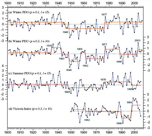
The following figure from the above paper show analysis of PDO and Victoria Index using the Rodionov regime detection algorithm. A regime shift is also detected around 1947-48.
The following figure shows regime shift detection for the summer PDO, showing shifts at 1948, 1976 and 1998.
[http://www.beringclimate.noaa.gov/data/Images/PDOs_FigRegime.html]
(For detailed information on the 1976/77 climate shift,
see: http://www.appinsys.com/GlobalWarming/The1976-78ClimateShift.htm)
Regime Shift Detection in Annual Temperature Anomaly Data
The NOAA Bering Climate web site provides the algorithm for regime shift detection developed by Sergei Rodionov [http://www.beringclimate.noaa.gov/regimes/index.html]. The following analyses use the Excel VBA regime change algorithm version 3.2 from this web site.
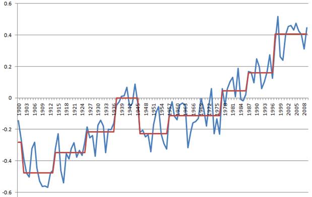
The following figure shows the regime analysis of the HadCRUT3 annual global annual average temperature anomaly data from the Met Office Hadley Centre for 1895 to 2009 [http://hadobs.metoffice.com/hadcrut3/diagnostics/global/nh+sh/annual].
The analysis was run based on the mean using a significance level of 0.1, cut-off length of 10 and Huber weight parameter of 2 using red noise IP4 subsample size 6. Regime changes are identified in 1902, 1914, 1926, 1937, 1946, 1957, 1977, 1987, and 1997. Running the analysis based on the variance rather than the mean results in regime changes in the bold years listed above.
Regime Shift Relationship to Solar Cycle
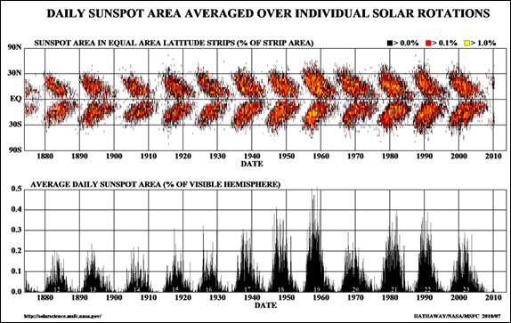
The NASA Solar Physics web site provides the following figure showing sunspot area.
[http://solarscience.msfc.nasa.gov/SunspotCycle.shtml]
The following figure compares the Hadley (HadCrut3) monthly global average temperature (from [http://hadobs.metoffice.com/hadcrut3/diagnostics/global/nh+sh/]) overlaid with the regime change line (red line) shown previously, along with the sunspot area since 1900. The sunspot cycle is approximately 11 years. The sun’s magnetic field reverses with each sunspot cycle and thus after two sunspot cycles the magnetic field has completed a cycle – a Hale Cycle – and is back to where it started. Thus a complete magnetic sunspot cycle is approximately 22 years. The figure marks the onset of odd-numbered cycles with a vertical red line, even-numbered cycles with a green line.
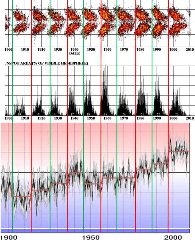
From the figure above it can be seen that the regime changes correspond to the onset of solar cycles and occur when the “butterfly” is at its widest. The most significant warming regime shifts occur at the start of odd-numbered cycles (1937, 1957, 1977, 1997). Each odd-numbered cycle (red lines above) has resulted in a temperature-increase regime shift. Even-numbered cycles (green lines above) have been inconsistent, with some resulting in temperature-decrease regime shifts (1902, 1946) or minor temperature-increase shifts (1926, 1987).
An unusual one is the 1957 – 1966 cycle, which in the monthly data shown above visually looks like a temperature-increase shift in 1957 followed by a temperature-decrease shift in 1964 but the regime detection algorithm did not identify it. This is likely due to the use of annually averaged data in the regime detection algorithm.
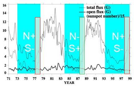
The following figure shows the relative polarity of the Sun’s magnetic poles for recent sunspot cycles along with the solar magnetic flux [www.bu.edu/csp/nas/IHY_MagField.ppt]. The regime change periods are highlighted by the red and green boxes. Each one occurs on as the solar cycle is accelerating. The onset of an odd-numbered sunspot cycle (1977-78, 1997-98) results in the relative alignment of the Earth’s and the Sun’s magnetic fields (positive North pole on the Sun) allowing greater penetration of the geomagnetic storms into the Earth’s atmosphere. “Twenty times more solar particles cross the Earth’s leaky magnetic shield when the sun’s magnetic field is aligned with that of the Earth compared to when the two magnetic fields are oppositely directed” [http://www.nasa.gov/mission_pages/themis/news/themis_leaky_shield.html]
The following figure shows the longitudinally averaged solar magnetic field. This “magnetic butterfly diagram” shows that the sunspots are involved with transporting the field in its reversal. The Earth’s temperature regime shifts are indicated with the superimposed boxes – red on odd numbered solar cycles, green on even.
[http://solarphysics.livingreviews.org/open?pubNo=lrsp-2010-1&page=articlesu8.html]
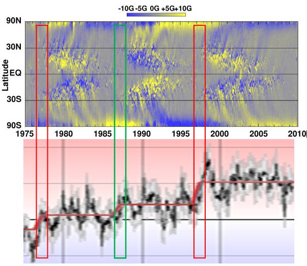
The Earth’s temperature regime shift occurs as the solar magnetic field begins its reversal.
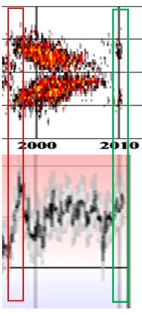
Solar Cycle 24
Solar cycle 24 is in its initial stage after getting off to a late start. An El Nino occurred in the first part of 2010. This may be the start of the next regime shift.
Climate Regime Shifts
[last update: 2010/07/04]
|
“The notion that climate variations often occur in the form of ‘‘regimes’’ began to become appreciated in the 1990s. This paradigm was inspired in large part by the rapid change of the North Pacific climate around 1977 [e.g., Kerr, 1992] and the identification of other abrupt shifts in association with the Pacific Decadal Oscillation (PDO) [Mantua et al., 1997].” [http://www.beringclimate.noaa.gov/regimes/Regime_shift_algorithm.pdf]
|
|
Pacific Regime Shifts
Hare and Mantua, 2000 (“Empirical evidence for North Pacific regime shifts in 1977 and 1989”): “It is now widely accepted that a climatic regime shift transpired in the North Pacific Ocean in the winter of 1976–77. This regime shift has had far reaching consequences for the large marine ecosystems of the North Pacific. Despite the strength and scope of the changes initiated by the shift, it was 10–15 years before it was fully recognized. Subsequent research has suggested that this event was not unique in the historical record but merely the latest in a succession of climatic regime shifts. In this study, we assembled 100 environmental time series, 31 climatic and 69 biological, to determine if there is evidence for common regime signals in the 1965–1997 period of record. Our analysis reproduces previously documented features of the 1977 regime shift, and identifies a further shift in 1989 in some components of the North Pacific ecosystem. The 1989 changes were neither as pervasive as the 1977 changes nor did they signal a simple return to pre-1977 conditions.” [http://www.sciencedirect.com/science?_ob=ArticleURL&_udi=B6V7B-41FTS3S-2…]
Overland et al “North Pacific regime shifts: Definitions, issues and recent transitions” [http://www.pmel.noaa.gov/foci/publications/2008/overN667.pdf]: “climate variables for the North Pacific display shifts near 1977, 1989 and 1998.”
The following figure from the above paper show analysis of PDO and Victoria Index using the Rodionov regime detection algorithm. A regime shift is also detected around 1947-48.
The following figure shows regime shift detection for the summer PDO, showing shifts at 1948, 1976 and 1998. [http://www.beringclimate.noaa.gov/data/Images/PDOs_FigRegime.html]
(For detailed information on the 1976/77 climate shift, see: http://www.appinsys.com/GlobalWarming/The1976-78ClimateShift.htm)
|
|
Regime Shift Detection in Annual Temperature Anomaly Data
The NOAA Bering Climate web site provides the algorithm for regime shift detection developed by Sergei Rodionov [http://www.beringclimate.noaa.gov/regimes/index.html]. The following analyses use the Excel VBA regime change algorithm version 3.2 from this web site.
The following figure shows the regime analysis of the HadCRUT3 annual global annual average temperature anomaly data from the Met Office Hadley Centre for 1895 to 2009 [http://hadobs.metoffice.com/hadcrut3/diagnostics/global/nh+sh/annual].
The analysis was run based on the mean using a significance level of 0.1, cut-off length of 10 and Huber weight parameter of 2 using red noise IP4 subsample size 6. Regime changes are identified in 1902, 1914, 1926, 1937, 1946, 1957, 1977, 1987, and 1997. Running the analysis based on the variance rather than the mean results in regime changes in the bold years listed above.
|
|
Regime Shift Relationship to Solar Cycle
The NASA Solar Physics web site provides the following figure showing sunspot area. [http://solarscience.msfc.nasa.gov/SunspotCycle.shtml]
The following figure compares the Hadley (HadCrut3) monthly global average temperature (from [http://hadobs.metoffice.com/hadcrut3/diagnostics/global/nh+sh/]) overlaid with the regime change line (red line) shown previously, along with the sunspot area since 1900. The sunspot cycle is approximately 11 years. The sun’s magnetic field reverses with each sunspot cycle and thus after two sunspot cycles the magnetic field has completed a cycle – a Hale Cycle – and is back to where it started. Thus a complete magnetic sunspot cycle is approximately 22 years. The figure marks the onset of odd-numbered cycles with a vertical red line, even-numbered cycles with a green line.
From the figure above it can be seen that the regime changes correspond to the onset of solar cycles and occur when the “butterfly” is at its widest. The most significant warming regime shifts occur at the start of odd-numbered cycles (1937, 1957, 1977, 1997). Each odd-numbered cycle (red lines above) has resulted in a temperature-increase regime shift. Even-numbered cycles (green lines above) have been inconsistent, with some resulting in temperature-decrease regime shifts (1902, 1946) or minor temperature-increase shifts (1926, 1987).
An unusual one is the 1957 – 1966 cycle, which in the monthly data shown above visually looks like a temperature-increase shift in 1957 followed by a temperature-decrease shift in 1964 but the regime detection algorithm did not identify it. This is likely due to the use of annually averaged data in the regime detection algorithm.
The following figure shows the relative polarity of the Sun’s magnetic poles for recent sunspot cycles along with the solar magnetic flux [www.bu.edu/csp/nas/IHY_MagField.ppt]. The regime change periods are highlighted by the red and green boxes. Each one occurs on as the solar cycle is accelerating. The onset of an odd-numbered sunspot cycle (1977-78, 1997-98) results in the relative alignment of the Earth’s and the Sun’s magnetic fields (positive North pole on the Sun) allowing greater penetration of the geomagnetic storms into the Earth’s atmosphere. “Twenty times more solar particles cross the Earth’s leaky magnetic shield when the sun’s magnetic field is aligned with that of the Earth compared to when the two magnetic fields are oppositely directed” [http://www.nasa.gov/mission_pages/themis/news/themis_leaky_shield.html]
The following figure shows the longitudinally averaged solar magnetic field. This “magnetic butterfly diagram” shows that the sunspots are involved with transporting the field in its reversal. The Earth’s temperature regime shifts are indicated with the superimposed boxes – red on odd numbered solar cycles, green on even. [http://solarphysics.livingreviews.org/open?pubNo=lrsp-2010-1&page=articlesu8.html]
The Earth’s temperature regime shift occurs as the solar magnetic field begins its reversal.
|
|
Solar Cycle 24
Solar cycle 24 is in its initial stage after getting off to a late start. An El Nino occurred in the first part of 2010. This may be the start of the next regime shift.
|
Thanks Leif,
I notice the abstact on the second link starts thusly:
“Butterfly diagrams (latitude-time plots) of coronal emission show a zone of enhanced brightness that appears near the poles just after solar maximum and migrates toward lower latitudes; a bifurcation seems to occur at sunspot minimum, with one branch continuing to migrate equatorward with the sunspots of the new cycle and the other branch heading back to the poles. The resulting patterns have been likened to those seen in torsional oscillations and have been taken as evidence for an extended solar cycle lasting over ~17 yr.”
Vuk I like your power spectrun graph. Tell us more about the individual lines and what they represent.
It ain’t mine, its doc Svalgaard’s. I added two orange lines which signify period and half–period now infamous anomaly equation:
http://www.vukcevic.talktalk.net/LFC4.htm
Dr S. I accept in advance as valid your comment as ‘Nothing to do with anything solar!’
tallbloke says:
July 12, 2010 at 11:22 am
Thanks Leif,
I notice the abstact on the second link starts thusly:
“[…]have been taken as evidence for an extended solar cycle lasting over ~17 yr.”
But note that the paper discounts that claim.
Here is a picture of the ‘extended cycle’: http://www.leif.org/research/Extended-Cycle.png
What is referred to is the fact that solar cycles overlap so that signs of the new cycle can be sign about a year before the ‘minimum’ and that old-cycle spots can be seen for about a year after minimum, making the cycles more like 13-14 year long. But the ‘overhang’ is not a particularly phenomenon in itself, and the ’17-year cycle’ as such is simply not in the data. True ‘cyclists’ might even claim that the 51-yr peak is the 17th sub-harmonic of a non-existent 3-yr peak as it being the 3rd subharmonic of a non-existent 17-yr peak. In cyclomania-world, everything is possible.
The pebbles Universe (Prof. Fred Flinstone) vs. the EU:
Twinkle, twinkle electric star
Astronomers don’t know what you are!
http://www.holoscience.com/news.php?article=x49g6gsf&keywords=white%20dwarf
Dr.Svalgaard (A.2)
If you look at your spectrum dip at 17 and 34 and peaks at 51 and 102.
Also dip at 24 ( 2 x J ), dip at 60 = 3 x 19, and so on.
Just look up resonant circuits, they absorb and give off power.
Enneagram says:
July 12, 2010 at 11:35 am
Astronomers don’t know what you are!
Astrologers do! or so they say.
Obviously the electric currents from the Universe are modulated by the planets, even the tiny ones [e.g. Ceres]…
Vuk etc. says:
July 12, 2010 at 11:40 am
If you look at your spectrum dip at 17 and 34 and peaks at 51 and 102.
Also dip at 24 ( 2 x J ), dip at 60 = 3 x 19, and so on.
Just look up resonant circuits, they absorb and give off power.
There are enough dips and peaks to satisfy any cyclist.
Circuits can only resonate if they are coupled.
I don’t mind if the sun runs on electricity, steam, burning obsolete textbooks or helium fusion. I just want to know how, and how much it affects Earth’s climate, how it relates to planetary motion, and what the likely variability is over various timescales.
Leif, I like your extended cycle. A correspondent recently showed me a very interesting graph which had a nice logical breakdown showing 5 overlapping 55 year cycles within the VEJ alignments producing peaks and troughs every 11 years. So I can see how one cycle ‘submerges’ over a couple of years as another ’emerges’. He also produced a graph which shows how these relate to the graph Ching Cheh Hung produced, and it shows the relationship between the planetary alignments and the solar cycles much more clearly, and to my eye irrefutably. There is a missing variable which I’m going to play with before I post it up though.
Exciting times for the planetologists. Hows the dynamology going?
tallbloke says:
July 12, 2010 at 11:55 am
Exciting times for the planetologists.
It has been exciting ever since Wolf [and others] proposed the idea 150 years ago, but nothing has come of all that excitement since.
Hows the dynamology going?
The sun is doing what it was predicted to do, so I think we are doing fine. At least we doing physics.
@Leif Svalgaard says:
July 12, 2010 at 10:33 am
“These claims are not substantiated by the data, so the period is not accepted as valid by the solar community. There are always lots of claims about cycles of every conceivable periods, but the data just isn’t there.”
There you go again, this is one claim about one cycle, and I would not take your word as to whether “these claims are substantiated by the data” or not. It would not be unconcievable for the whole orthodox solar community to have failed to analize the data correctly.
Leif Svalgaard says:
July 12, 2010 at 11:58 am
It has been exciting ever since Wolf [and others] proposed the idea 150 years ago, but nothing has come of all that excitement since.
The sun is doing what it was predicted to do, so I think we are doing fine. At least we doing physics.
I’m glad you are. I expect we’ll be meeting further down the road when the obvious planetary connection eventually forces physicists with fine abilities such as yours to come up with the details of the viable mechanism I’ve intuited.
Ulric Lyons says:
July 12, 2010 at 12:14 pm
this is one claim about one cycle
And in particular, the data is not there to support that one claim, either
It would not be unconcievable for the whole orthodox solar community to have failed to analize the data correctly.
OK, Einstein, we are awaiting your correct analysis.
tallbloke says:
July 12, 2010 at 12:18 pm
physicists with fine abilities such as yours to come up with the details of the viable mechanism I’ve intuited.
Another Einstein here?
meeting further down the road when the obvious planetary connection…
It has been ‘obvious’ for 150 years. I may not live long enough.
Lol, I hope you do Leif. Better watch the waistline though, there will be much humble pie to be eaten. 😉
tallbloke says:
July 12, 2010 at 12:58 pm
there will be much humble pie to be eaten. 😉
I’ll be glad to serve up your portion.
Dr. Svalgaard (A.2)
Of course they are coupled; 5J = 59.31, 2S = 59.31. Any astronomer it will tell you that every time J ( 19.6 yrs) passes Sn-St line it gives a tiny nudge to St.
4.5 billion/19.6 is a lot of nudges, and they were much stronger in the early aeons, long before von Helmholtz ‘hit the bottle’ (with a hummer I mean).
Leif Svalgaard says:
July 12, 2010 at 1:19 pm (Edit)
I’ll be glad to serve up your portion.
I’ll bring the cream.
Just had a hit from your esteemed colleagues:
Location: Cambridge, Massachusetts, United States
IP Address: Harvard-smithsonian Center For Astrophysics (131.142.188.56) [Label IP Address]
Entry Page: http://www.vukcevic.talktalk.net/NATA.htm
Exit Page: http://www.vukcevic.talktalk.net/LFC-CETfiles.htm
Referring URL: No referring link
Watch out Vuk, next they’ll either be stealing your ideas, or your trash bag.
Vuk etc. says:
July 12, 2010 at 1:25 pm
Of course they are coupled
But not to where it matters for the topic at hand: the Sun.
tallbloke: You asked, “Have you got a reliable longer list of El ninos I can test against more solar cycles? The more samples we test, on a longer timescale the more certain the outcome.”
Depends on your definition of reliable. There are a number of ENSO-related reconstructions on the NOAA Paleoclimatology Program webpage, under the heading of Circulation, (subheading Pacific):
http://www.ncdc.noaa.gov/paleo/recons.html#circulation
This is wrong, and a perfect example of lack of scrutiny:
http://www.leif.org/research/FFT%20of%20IMF%20Direction.png
the peak just before 200 days is not semi annual, that would be nearer 182 days.
As all solar/climate/weather periods can be mapped out precisely by planetary harmonies, this period should be c.194.6 days, 1/12 of the 6.395yr harmony of Earth, Mars, Venus and Ceres, a half J/N synod, and two bashful ballerina`s.
Leif Svalgaard says:
July 12, 2010 at 11:53 am (Edit)
Circuits can only resonate if they are coupled.
Yep, like Earth and Venus are with Jupiter, and Jupiter is with Saturn, and Saturn is with Neptune. The lower integers in the fibonacci series keep popping out all over the place. Five conjunctions of Earth and Venus over an eight year cycle etc.
The whole solar system resonates, and many of the frequencies are evident in the sun as discovered by magnetohydrodynamics studies.the outer planets lie at the nodes of a 168 minute lightspeed wave centred on the sun. This number crops up all over the galaxy.
I wish I understood why Leif and so many of his colleagues are so resistant to the study of waves and cycles. Maybe it’s just too analogue for them in the high speed digitally quantised age.
tallbloke says:
July 12, 2010 at 1:56 pm
I wish I understood why Leif and so many of his colleagues are so resistant to the study of waves and cycles.
We are not. In fact, we are great experts on this. Just think of the modern field of helioseismology. And on the Kirkwood gaps between asteroids and in the rings of Saturn. And on Alfven wave interactions. And on cosmic ray scattering.
The issue has several aspects:
1) the time scale [must match]
2) the energy [must match]
3) the coupling mechanism [must be viable – e.g. the ‘angular momentum theory’ is not]
But we have gone over that so many times to no avail, that it is hardly worth the trouble to re-hash any of that here.
Your other stuff is [“magnetohydrodynamics studies”,”168 minute lightspeed wave”, “all over the galaxy”] is just nonsense.
I make it 6216 days for an average coronal hole cycle, Vuk reckons 6189 days, either way, it is the last BIG spike in the graph:
http://www.leif.org/research/FFT%20of%20IMF%20Direction.png